A radio-jet driven outflow in the Seyfert 2 galaxy NGC 2110?

We present a spatially-resolved study of the ionised gas in the central 2 kpc of the Seyfert 2 galaxy NGC 2110 and investigate the role of its moderate luminosity radio jet (kinetic radio power of $P_{\mathrm{jet}}=2.3\times 10^{43}\ \mathrm{erg\,s^{-1}}$). We use new optical integral-field observations taken with the MEGARA spectrograph at the Gran Telescopio Canarias, covering the $4300-5200\,\AA$ and $6100-7300\,\AA$ ranges with a spectral resolution of $R\simeq 5000-5900$. We fit the emission lines with a maximum of two Gaussian components, except at the AGN position where we used three. Aided by existing stellar kinematics, we use the observed velocity and velocity dispersion ($\sigma$) of the emission lines to classify the different kinematic components. The disc component is characterised by lines with $\sigma\simeq 60-200\,\mathrm{km\,s}^{-1}$. The outflow component has typical values of $\sigma\simeq 700\,\mathrm{km\,s}^{-1}$ and is confined to the central $2.5\arcsec\simeq 400\,$pc, which is coincident with linear part of the radio jet detected in NGC 2110. At the AGN position, the [O III]$\lambda$5007 line shows high velocity components reaching at least $1000\,\mathrm{km\,s}^{-1}$. This and the high velocity dispersions indicate the presence of outflowing gas outside the galaxy plane. Spatially-resolved diagnostic diagrams reveal mostly low ionisation (nuclear) emitting region (LI(N)ER)-like excitation in the outflow and some regions in the disc, which could be due to the presence of shocks. However, there is also Seyfert-like excitation beyond the bending of the radio jet, probably tracing the edge of the ionisation cone that intercepts with the disc of the galaxy. NGC 2110 follows well the observational trends between the outflow properties and the jet radio power found for a few nearby Seyfert galaxies. All these pieces of information suggest that part of observed ionised outflow in NGC 2110 might be driven by the radio jet. However, the radio jet was bent at radial distances of $\sim 200\,$pc (in projection) from the AGN, and beyond there, most of the gas in the galaxy disc is rotating.

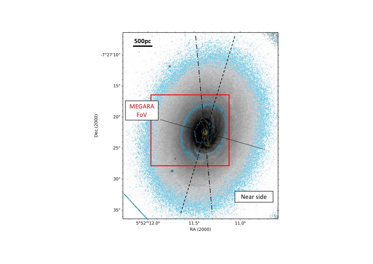
Figure 1: HST/WFPC2 optical image of NGC 2110 obtained with the F791W filter, shown on a linear scale (grey colors and blue contours). The orange contours (also on a linear scale) are the VLA radio 6 cm emission from Ulvestad & Wilson (1983). We also mark with a red rectangle the approximate size of the GTC/MEGARA FoV of $12.5\arcsec\times 11.3\arcsec$. The dashed and dotted lines are the position angle of the galaxy major axis (PA $\simeq 163^{\circ}$ measured from the north to the east, see Ferruit et al., 2004) and the minor axis, respectively. The dashed-dotted line is the PA of the slit used by González Delgado et al. (2002) and discussed in Sect. 3.3.

1 Introduction

Active galactic nuclei (AGN) are crucial for understanding galaxy evolution. AGN feedback has been proposed as one mechanism to reproduce the observed number of the most massive galaxies, because in its absence star formation would have been too efficient (e.g., Silk & Mamon, 2012). In particular, in moderate luminosity AGN, the relationship between radiation driven outflows and radio jets remains as an open problem. From the theoretical point of view, it is expected that galaxies hosting radio jets could drive outflowing material (e.g., Weinberger et al., 2017; Mukherjee et al., 2018; Talbot et al., 2022; Meenakshi et al., 2022). From the observational side, the capacity of high power radio jets to produce energetic outflows is well demonstrated (e.g., Nesvadba et al., 2008; Vayner et al., 2017).

The impact of low to moderate luminosity radio jets on the interstellar medium (ISM) of their host galaxies has been studied mostly in local Seyfert galaxies, low-luminosity AGN, and quasars. It has been shown that in the presence of a good geometrical coupling, these jets can transfer successfully mechanical energy to the ISM of their host galaxies (e.g., Combes et al., 2013; García-Burillo et al., 2014; Morganti et al., 2015; García-Bernete et al., 2021; Maccagni et al., 2021; Pereira-Santaella et al., 2022; Cazzoli et al., 2022; Speranza et al., 2022; Audibert et al., 2023). Using a small sample of Seyfert galaxies, Venturi et al. (2021) detected enhanced widths of optical lines in regions perpendicular to the radio jet, while Seyfert-like excited conical shapes were aligned with the radio jet. They interpreted this as the result of the interaction between the radio jet and outflowing material. In this context, they proposed scaling relationships between both the ionised gas mass and kinetic energy in the regions with enhanced line width and the radio jet power.

NGC 2110 is an early type spiral galaxy (SAB0) hosting a Seyfert 2 nucleus (McClintock et al., 1979), observed at an intermediate inclination $i=42-65^{\circ}$ (see e.g., Wilson & Baldwin, 1985; González Delgado et al., 2002; Kawamuro et al., 2020, and Fig. 1). It contains a radio jet, whose ‘S’-shaped jet was proposed to be the result of its bending by the ram pressure of the host galaxy rotating gas (Ulvestad & Wilson, 1983). The jet appears brighter on the north side, which allowed Pringle et al. (1999) to estimate that it is at an intermediate orientation with respect to the plane of the galaxy. The luminosity of this jet lies at the high end of the 20 cm radio luminosity distribution of the early-type Seyfert galaxies studied by Nagar et al. (1999).

Several works studied NGC 2110 in detail using optical integral field unit (IFU) spectroscopy (González Delgado et al., 2002; Ferruit et al., 2004; Schnorr-Müller et al., 2014) with spectral resolutions $R=\lambda$/$\Delta\lambda\simeq 1000-2000$. They all detected the presence of complex non-circular motions in the ionised gas, which were interpreted as due to the presence of an outflow, inflow, and/or a minor merger. Moreover, Rosario et al. (2010) demonstrated that the radio jet has sufficient ram pressure to drive the emission-line outflow. Finally, using Atamaca Large Millimeter Array (ALMA) CO(2-1) observations, Rosario et al. (2019) discovered a nuclear region with faint cold molecular gas emission (termed “lacuna”), which is oriented in the approximate direction of the radio jet and filled with warm molecular hydrogen emission. These authors suggested that the radio jet and/or an AGN wind could be responsible for this phenomenon.

Table 1: Parameters employed for the construction of cubelets and their line fits.

Cubelet name	Rest-frame wavelength range	Rest-frame continuum regions	AoN	$A_{\mathrm{min}}$
	(Å)	(Å)		(10-18 erg s-1 cm-2 Å-1)
H$\beta$	4800–4920	4800–4820, 4900–4920	1.5	4.0
[O III]$\lambda\lambda$4959, 5007	4900–5065	4900–4920, 5045–5065	2.0	4.0
[O I]$\lambda$6300	6255–6345	6255–6275, 6325–6345	1.5	3.0
H$\alpha$ + [N II]$\lambda\lambda$6548, 6583	6475–6640	6475–6495, 6620–6640	2.0	7.0
[S II]$\lambda\lambda$6716, 6731	6660–6780	6660–6680, 6760–6780	2.0	4.0

As part of the Galactic Activity, Torus, and Outflow Survey (GATOS), we obtained new optical IFU observations of several Seyfert galaxies, including NGC 2110 using the Multi-Espectrógrafo en GTC de Alta Resolución para Astronomía (MEGARA, Gil de Paz et al., 2016; Carrasco et al., 2018) at the 10.4-m Gran Telescopio Canarias (GTC) with $R=5000-5900$. Our observations cover the $\sim$4300–5200 $\AA$ and $\sim$6100–7300 $\AA$ spectral ranges, which allow us to spatially resolve both the gas kinematics and the excitation mechanisms in NGC 2110. By revisiting this well-studied target, we plan to use it as a benchmark for other forthcoming analyses of MEGARA observations within the GATOS survey.

This paper is structured as follows. Section 2 describes the data employed in this work. Section 3 explains the analysis, the classification of gas components, and the construction of the two-dimensional maps. We discuss the properties of the disc and outflow regions of NGC 2110 in Sects. 4 and  5, respectively. Finally, the summary and conclusions are presented in Sect. 6. We assume a systemic velocity of $2335\pm 20\,$km s^-1, based on measurements of stellar absorptions from the magnesium $b$ triplet at $\sim$5175 Å by Nelson & Whittle (1995). We adopt a $\Lambda$ cold dark matter cosmology with $H_{0}$=70 km s^-1 Mpc^-1, $\Omega_{\mathrm{m}}$=0.3, and $\Omega_{\Lambda}$=0.7, which leads to a luminosity distance of $D_{L}=33.6\,$Mpc and a physical scale of $160.2\,\mathrm{pc}/\arcsec$.

2 Observations

2.1 Optical IFU data from MEGARA

We observed the central region of NGC 2110 (Program GTC27-19B, PI: Alonso Herrero) using the large compact bundle (LCB) of fibers of MEGARA (i.e., the IFU mode of this instrument). This IFU provides a field of view (FoV) of $12.5\arcsec\times 11.3\arcsec$ (see Fig. 1), using 567 fibers of $0.62\arcsec$ in diameter. The physical region covered for NGC 2110 by our MEGARA observations is 2.0 $\times$ 1.8 kpc². We used two volume-phased holographic gratings. The LR-B grating covers the spectral range $\sim$4300–5200 $\AA$ with $R\sim$5000. H$\beta$ and the [O III]$\lambda\lambda$4959, 5007 doublet are within this range for NGC 2110. The LR-R grating covers the $\sim$6100–7300 $\AA$ range with $R$ $\sim$ 5900, thus including [O I]$\lambda$6300, H$\alpha$, [N II]$\lambda\lambda$6548, 6583 and [S II]$\lambda\lambda$6716, 6731. The on-source integration times were $\sim$1 hour (7 exposures of 520 s each) for LR-B and half hour (5 exposures of 360 s each) for LR-R.

The observations were taken in two consecutive observation blocks on the night of 9^th February 2021. The observing conditions were a dark photometric sky and a seeing of $0.9\arcsec$. The position angle (PA) of the observations was $-0.598\degr$, which is practically equivalent to the regular orientation north up, east to the left.

The data reduction was performed using the official MEGARA pipeline (Pascual et al., 2021). The data reduction process of this software includes bias subtraction, bad-pixels masking, tracing fibres, wavelength calibration (including versions corrected and uncorrected of barycentric velocity), flat-field correction, flux calibration, sky subtraction and cube construction. The flat-field images were taken with a continuum halogen lamp and close in time to the target exposures. This allows us to use them for tracing fibres without dealing with their known shifts that depend on the ambient temperature. Also just before the target exposures, we obtained images illuminated with a Thorium-Argon hollow cathode lamp, which were used for the wavelength calibration. The spectrophotometric standard star HR 1544/HR 4554 was used for the flux calibration of the observations with the LR-B/LR-R grating. The final data cubes were produced with $0.3\arcsec$ spaxels, which is the recommended size by the pipeline developers.

We note that NGC 2110 was also observed as part of the Siding Spring Southern Seyfert Spectroscopic Snapshot Survey (S7; Thomas et al., 2017), using the WiFeS instrument on the ANU 2.3-m telescope. Although their FoV is larger ($25\arcsec\times 38\arcsec$) than that provided by MEGARA, our data have higher spatial resolution due to both the smaller MEGARA fiber diameter ($0.62\arcsec$) versus the S7 spaxel ($1\arcsec\times 1\arcsec$) and better seeing conditions (MEGARA $0.9\arcsec$ versus S7 $1.4\arcsec$). In addition, our MEGARA observations have higher spectral resolution in the blue range (5000 versus 3000 for the S7 survey).

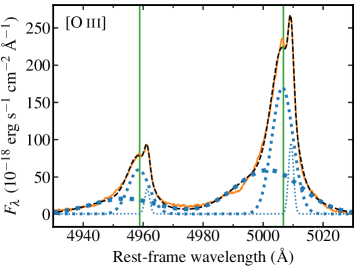
Figure 2: GTC/MEGARA nuclear spectrum of NGC 2110 in the spectral region around the [O III]$\lambda\lambda$4959, 5007 doublet. The orange line is the observed spectrum after the subtraction of the continuum and extracted with a $0.9\arcsec\times 0.9\arcsec$ aperture. The fit (black dashed line) is the sum of three Gaussian components. The blue dotted lines show each component of the fit, with lines of increasing thickness for the components with increasing velocity dispersions. The green lines are the line wavelengths.

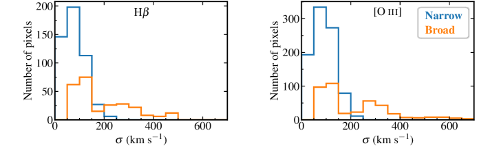
Figure 3: Observed distribution of the velocity dispersions (corrected for the instrumental resolution) fitted on a spaxel-by-spaxel basis and using a maximum of two Gaussian components from lines observed with the GTC/MEGARA LR-B grating, i.e., H$\beta$ and [O III]$\lambda\lambda$4959, 5007 lines. Blue and orange lines correspond to the narrow and broad components, respectively (see text).

As the absolute flux calibration has a direct impact on the outflow properties (Sect. 5.4), we compare our calibration with those provided by other authors. Davies et al. (2020) presented Very Large Telescope (VLT) X-Shooter observations of NGC 2110 and measured observed fluxes (not corrected for extinction) of 7.85 $\pm$ 0.10 $\times$ $10^{-15}$ erg s^-1 cm^-2 and 41.1 $\pm$ 0.5 $\times$ $10^{-15}$ erg s^-1 cm^-2 for the H$\beta$ and H$\alpha$ lines for an aperture of $1.8\arcsec\times 1.8\arcsec$ under seeing conditions ranging between $0.50\arcsec$ and $0.58\arcsec$. We reproduced their aperture on our GTC/MEGARA data and we obtained 25.6 $\times$ $10^{-15}$ erg s^-1 cm^-2 and 101.8 $\times$ $10^{-15}$ erg s^-1 cm^-2, respectively. Thomas et al. (2017), as part of the S7 survey, reported a dereddened flux of 384.8 $\times$ $10^{-15}$ erg s^-1 cm^-2 for the H$\beta$ line for a circular $4\arcsec$ diameter aperture and a seeing of $1.4\arcsec$. Undoing the dereddening in the same way as these authors (i.e., a Fitzpatrick 1999 reddening law with $R_{V}$=3.1 and $A_{V}$=2.39 mag) leads to a non-dereddened flux of 29.5 $\times$ $10^{-15}$ erg s^-1 cm^-2. We extracted a spectrum with the same aperture from our IFU data and we obtained a flux of 45.1 $\times$ $10^{-15}$ erg s^-1 cm^-2.

It is worth mentioning that both works subtracted the stellar continuum from their spectra before measuring the line fluxes. Consequently, we also subtracted the stellar continuum around H$\beta$ line for the above estimates (see Sect. 3), while that correction was assumed negligible for H$\alpha$. However, we noticed that the selection of stellar continuum template contributes significantly to these differences. For instance, the above value for the comparison with Thomas et al. (2017) was obtained using the stellar fit by Burtscher et al. (2021), while using the one from Davies et al. (2020) leads to a non-dereddened H$\beta$ flux of 38.1 $\times$ $10^{-15}$ erg s^-1 cm^-2, and when the stellar continuum is not subtracted, we found 37.7 $\times$ $10^{-15}$ erg s^-1 cm^-2 (see Sect. 3 for more details about stellar continuum templates). In summary, our absolute flux calibration is 2.5 and 3.3 times higher than the estimates by Davies et al. (2020) for the H$\beta$ and H$\alpha$ lines, respectively. However, it is only 20-50 per cent higher for H$\beta$ than that of the larger apertures used by Thomas et al. (2017). Part of the differences with Davies et al. (2020) might be attributed to centering differences.

Additionally, we checked that our relative flux calibration within each of the GTC/MEGARA gratings provides similar line ratios to those in Davies et al. (2020). We measured [O III]$\lambda$5007/H$\beta$=4.96 and [N II]$\lambda$6583/H$\alpha$=1.62 using the same aperture as these authors, while they reported a value of 4.76 and 1.37 for these same ratios. In what follows, we will use our own flux calibration throughout this work and take into account the uncertainty in the absolute calibration when needed.

2.2 Ancillary radio observations

In order to interpret our MEGARA observations and their potential relationship with the radio jet of NGC 2110, we downloaded from NASA/IPAC Extragalactic Database (NED) a radio map observed at 6 cm (4885 MHz) by Ulvestad & Wilson (1983, 1984, 1989). These observations were taken on 15^th March 1982, using the A configuration of the Very Large Array (VLA) at the National Radio Astronomy Observatory. The observations consisted of two exposures of 12 minutes each. Calibration and self-calibration of the data followed the standard procedures (e.g., Wilson & Ulvestad, 1982). The radio map has a half-power beam width of $0.44\arcsec\times 0.35\arcsec$ at a PA$=-1\degr$.

Ulvestad & Wilson (1983) found that the optical nucleus (observed by Clements, 1983) and the central radio component were coincident. We retrieved an optical image of NGC 2110 from ESASky (Baines et al., 2017; Giordano et al., 2018). The observations were taken with the Hubble Space Telescope (HST) WFPC2 instrument using the F791W filter. We adjusted the HST astrometry using the Gaia information from stars in the field and found that the positions of the nuclear radio and optical peaks agreed with each other, as can be seen from Fig. 1. This fact allowed us to assume that both the MEGARA continuum peak and the VLA peak mark the position of the AGN.

3 Analysis of the MEGARA observations

3.1 Emission line fitting

For the analysis of the emission lines of the MEGARA IFU data of NGC 2110, we developed a new Python tool named ALUCINE. This Spanish acronym stands for Ajuste de Líneas para Unidades de Campo Integral de Nebulosas en Emisión or IFU line fitting for emission-line nebulae. This is a general purpose tool designed to fit emission lines in integral-field data, using a user-specified number of components. At each spaxel, the fit of the line (or lines) is performed automatically and independently. We already used this tool with IFU observations obtained with the MIRI instrument on the James Webb Space Telescope (see García-Bernete et al., 2022).

Before we fitted the emission lines of the MEGARA observations, we subtracted the stellar continuum around the H$\beta$ region (i.e,. within the wavelength range stated for that line in Table 1) from the LR-B cube on a spaxel-by-spaxel basis. This is especially important for the H$\beta$ emission line fluxes since they are affected by stellar absorption, while it was assumed negligible for the other emission lines. We tried three different approaches, namely, subtracting the stellar templates provided by Burtscher et al. (2021) and Davies et al. (2020), and not subtracting any template. In particular, when subtracting a stellar template we scaled it to match the continuum level measured in the H$\beta$ continuum region (defined in Table 1) for each spaxel. For the figures included in this work and all the subsequent analysis, we made the correction with the template provided by Burtscher et al. (2021). However, it is worth mentioning that we checked that results of this work are not affected if we used the template from Davies et al. (2020) or even if we did not subtract the stellar continuum. For the LR-R data cube, we did not subtract a stellar template. However, the impact of this correction on the H$\alpha$ fluxes and [N ii]/H$\alpha$ line ratios is reduced when compared with H$\beta$ and line ratios involving this line because H$\alpha$ is brighter. Moreover, Bellocchi et al. (2019) demonstrated that the effects of the stellar template on the gas H$\alpha$ kinematics were not critical.

In what follows, we describe the steps followed to perform the line fitting of our MEGARA observations.

1. We spatially smoothed the cubes. Specifically, we assigned to each spaxel the mean value in a square box of 3 spaxels ($0.9\arcsec\times 0.9\arcsec$) around it. We chose this size for the box because it corresponds to the seeing value of the observations.

2. We built cubelets from the MEGARA cubes, i.e., we created smaller cubes by cutting spectral slices of the cubes covering the emission lines to be analysed. The resulting five cubes and their wavelength ranges are listed in Table 1.

3. We estimated the noise in each spaxel of each cubelet using regions where the continuum level is flat. These continuum regions are detailed in Table 1.

4. Given the good quality of the GTC/MEGARA observations, we fitted independently the emission line(s) at each spaxel of each cubelet. Thus, the method does not assume that all the emission lines share the same kinematics. We allowed for a maximum of two Gaussian components.

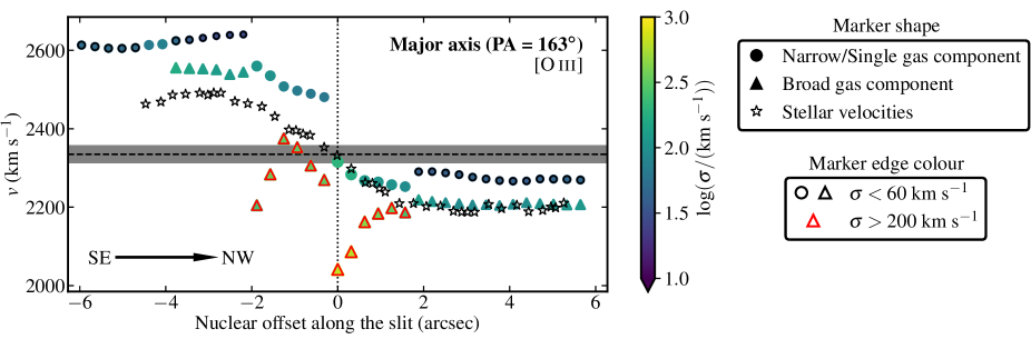
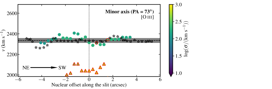
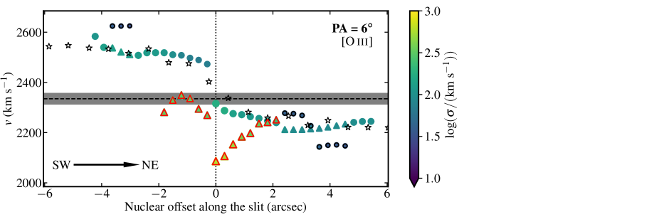
Figure 4: Comparison between the velocities of the ionised gas derived from fits using a maximum of two Gaussian components for the [O III]$\lambda\lambda$4959, 5007 doublet and the stellar velocities. From top to bottom, the stellar velocities are along the major and minor axes of the galaxy from Ferruit et al. (2004) and along PA=$6^{\circ}$ from González Delgado et al. (2002). Circles represent the narrow component or that when only one Gaussian is required to fit the line, while triangles correspond to the broad component. Stars show stellar velocities. The colour and size of circles and triangles depend on the velocity dispersion of each component. Black/Red edges have been added to the circles/triangles for velocity dispersions below/above 60/200 km s^-1, in order to illustrate the component classification explained in Sect. 3.1. The horizontal dashed line shows the systemic velocity, while the horizontal grey region its error.

In ALUCINE, the number of components to fit the emission lines at each spaxel is decided as follows. We started with zero components by default. If we detected a line above a specified threshold on amplitude over noise (AoN, see below), we tried to fit it and we trusted the resulting fit if it had a specified value of the minimum amplitude ($A_{\mathrm{min}}$). In the case of having added one component, we iterated the criteria starting from the residual derived from the previous fit. The values of AoN and $A_{\mathrm{min}}$ were tuned for each cubelet, seeking a compromise between maximising the signal and minimising the noise in the resulting maps. The final values of these two parameters for each cubelet are listed in Table 1. We should highlight that, if AoN values in this table were set to a value of 3.0, only a few spaxels would be affected by this change. This is because the cuts introduced by the $A_{\mathrm{min}}$ values do in practice also mean that spaxels with low AoN are not fitted. The fitting model (e.g., the number of Gaussians or other line profiles) depends on the cubelet and the nature of each emission line. In particular for the MEGARA data sets, we used a baseline for adjusting the continuum level plus the following models:

• H$\beta$: Each component for this singlet is one Gaussian with three free parameters, namely, amplitude, central wavelength, and line width.

• [O III]$\lambda\lambda$4959, 5007: Each component for this doublet is a set of two Gaussians sharing the same kinematics and with a fixed ratio between amplitudes of $A_{\mathrm{[{O\textsc{III}}]\ \lambda 4959}}=0.350\ A_{\mathrm{[{O\textsc{III}}]\ \lambda 5007}}$.

• [O I]$\lambda$6300: Although this line is a doublet with that at 6364 Å, they are well separated in our GTC/MEGARA spectra. Moreover, the latter line is not close to any other line of interest in this work. We therefore decided to fit only the [O I]$\lambda$6300 line.

• H$\alpha$ + [N II]$\lambda\lambda$6548, 6583: Each component for these lines is a set of three Gaussians. Two share the same kinematics and have an amplitude ratio of $A_{\mathrm{[{N\textsc{II}}]\ \lambda 6548}}=0.340\ A_{\mathrm{[{N\textsc{II}}]\ \lambda 6583}}$ in order to fit the [N II]$\lambda\lambda$6548, 6583 doublet. The third Gaussian fits the H$\alpha$ line with its own three free parameters. The amplitude of the H$\alpha$ line is that employed to evaluate if it passes the threshold value $A_{\mathrm{min}}$ explained above.

• [S II]$\lambda\lambda$6716, 6731: Each component for this doublet is a set of two Gaussians sharing the same kinematics and the ratio between amplitudes of them is a free parameter.

When fitting the lines with a particular model, we imposed a constraint that the fitted lines had widths equal to or higher than the instrumental resolution of our data, that is, 0.78 Å  at full width at half maximum (FWHM) for the LR-B grating and 1.0–1.1 Å  for the LR-R grating. As ALUCINE also allows the user to apply limits to the velocities and line widths, we used this feature to a fix spurious fits of the lines in a few spaxels. This did not affect the results when compared to those provided with the fits without this fine tuning.

We decided to use a maximum of two Gaussian components because they provided good quality fits to the emission lines in most of the spaxels of our MEGARA observations. In the nuclear region of NGC 2110, we nevertheless found that a three Gaussian component fit gave a significantly better performance. In Fig. 2, we show this fit for a spectrum extracted with a $0.9\arcsec\times 0.9\arcsec$ aperture and the [O III]$\lambda\lambda$4959, 5007 doublet. The fits for the rest of the emission lines can be seen in Appendix A. Table 2 lists the fluxes, velocities, and velocity dispersions for each of the three components for all the emission lines.

Table 2: Measurements from the nuclear spectrum using a model with three Gaussian components.

Emission line	$F_{1}$ / $F_{2}$ / $F_{3}$	$v_{1}$ / $v_{2}$ / $v_{3}$	$\sigma_{1}$ / $\sigma_{2}$ / $\sigma_{3}$
	$(10^{-18}\ \mathrm{erg\ s^{-1}\ cm^{-2}})$	$(\mathrm{km\ s^{-1}})$	$(\mathrm{km\ s^{-1}})$
H$\beta$	403 / 254 / 44	-47 / -3 / 137	487 / 178 / 60
[O III]$\lambda$5007	1632 / 1495 / 200	-317 / -27 / 144	662 / 210 / 46
[O I]$\lambda$6300	1131 / 504 / 93	-34 / 27 / 151	443 / 157 / 49
H$\alpha$	1182 / 1273 / 316	-281 / 7 / 142	339 / 172 / 55
[N II] $\lambda$6583	2855 / 1558 / 325	-202 / 31 / 156	446 / 161 / 50
[S II] $\lambda$6716	973 / 301 / 392	4 / -8 / 150	264 / 90 / 62
[S II] $\lambda$6731	1012 / 256 / 292	4 / -8 / 150	264 / 90 / 62

3.2 Distributions of the fitted velocity dispersions

As explained in Sect. 3.1, we fitted the optical emission lines with one or two components on a spaxel-by-spaxel basis. We termed them narrow and broad (see below) when two Gaussian components were fitted, and narrow if one Gaussian component provided a good fit. Figures 3 and 18 show the distribution of the velocity dispersions, corrected for instrumental resolution, for H$\beta$ and [O III]$\lambda\lambda$4959, 5007, and [O I]$\lambda$6300, H$\alpha$, [N II]$\lambda\lambda$6548, 6583 and [S II]$\lambda\lambda$6716, 6731, respectively.

The velocity dispersion distributions for the narrow component are narrow and clearly unimodal, peaking at 50–100 km s^-1. These values are similar to the values derived from VLT/MUSE observations for other Seyfert 2 galaxies, like NGC 5643 (García-Bernete et al., 2021) and NGC 7130 (Comerón et al., 2021). Regarding the broad component, most of the distributions tend to be bimodal, with one peak with velocity dispersions at $100-150$  km s^-1, thus broader than the narrow component. The second peak of the broad component is at $\sigma\sim$200–350 km s^-1, followed by a tail towards high velocity dispersions. The latter reaches values of up to $\sim$500–700 km s^-1, mostly in [O III]$\lambda\lambda$4959, 5007 and [N II]$\lambda\lambda$6548, 6583. The distributions of the fitted velocity dispersions in the MEGARA LR-R data cube are similar to those of Schnorr-Müller et al. (2014).

3.3 Comparison with the stellar kinematics

To classify the different ionised gas components according to their kinematics, in this section we compare the gas velocities with those measured from stellar absorption features. Figure 4 shows the velocities of the two components fitted for the [O III]$\lambda$5007 line versus the stellar kinematics along three different slit PAs. The top and middle panels are the stellar kinematics along the galaxy major (PA=$163^{\circ}$) and minor (PA=$73^{\circ}$) axes from Ferruit et al. (2004), while the bottom panel is along PA=$6^{\circ}$ from González Delgado et al. (2002). For reference, we show the orientation of these slits in Fig. 1.

Figure 4 already reveals the difficulty in classifying the different ionised gas kinematic components in NGC 2110. Along the NGC 2110 major axis, our MEGARA observations detected two components out to a radial distance of approximately $4\arcsec$ to the southeast and $6\arcsec$ to the northwest. Along the minor axis, the two components are seen in the inner $\sim 4\arcsec$. In this central region and along the minor axis, the [O III] narrow component follows relatively well the stellar kinematics (middle panel of Fig. 4). When comparing with the stellar kinematics of González Delgado et al. (2002) along PA=$6^{\circ}$, the ionised gas component with the intermediate velocity dispersions agrees well with the stars (bottom panel of Fig. 4).

Along the major axis of the galaxy to the northwest and in the central $\sim 2\arcsec$, the velocities of the gas narrow component are comparable to those of the stars, while beyond $2\arcsec$ they are redshifted. To the southeast the gas velocities are redshifted with respect to those of the stars (top panel of Fig. 4). This is similar to the findings of Ferruit et al. (2004). The broad component with $\sigma\simeq 250-670\,\mathrm{km\,s}^{-1}$ in the inner $4\arcsec$ is likely tracing an outflow, which we will analyse in more detail in Sect. 5. In the outer regions to the northwest and along the galaxy major axis, the component with intermediate values of velocity dispersion traces well the stellar kinematics. The narrowest gas component (circles in the figure) to the southeast at radial distances $>2\arcsec$ deviates the most from the stellar velocities, with gas velocities faster than the stellar ones.

A plausible scenario accounting for a slower rotation of the stars relative to the gas in some parts of the galaxy would invoke a rotation lag in thick stellar discs or a comparatively larger contribution of the velocity dispersion in the stellar component. However, the behaviour is the opposite in the northwest side. Here, the reported asymmetry of the gas kinematics in NGC 2110 could be explained by an uneven impact left by the radio jet on the gas motions, which probably slowed down the gas with the lowest observed velocity dispersions on the northern side of the disc. The secondary peak of the ALMA millimeter emission (see panel (c) of Figure 1 of Rosario et al., 2019) identifies the region where the jet was probably diverted. We will discuss the impact of the radio jet in more detail in Sect. 5.5.

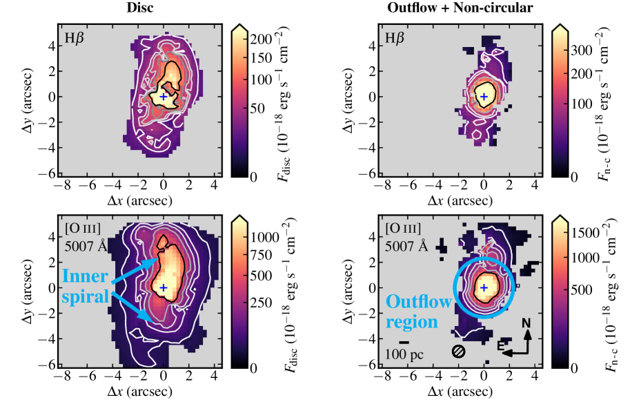
Figure 5: Flux maps of the disc (left) and the outflow+non-circular (right) components for the lines observed with the GTC/MEGARA LR-B grating, i.e., the H$\beta$ and [O III]$\lambda$5007 lines. All the colour bars use a square root scale and are saturated at the half maximum value of each map. Contour levels correspond to 30, 60, 70, 80 and 90 per cent of the maximum value of each map. Crosses indicate the location of the nucleus (as defined by the peak of the continuum). The north-east compass, the hatched circle indicating the seeing size, and physical size bar at the bottom right map apply to all the maps.

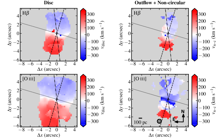
Figure 6: Velocity maps of the disc (left) and the outflow+non-circular (right) components for the lines observed with the GTC/MEGARA LR-B grating, i.e., H$\beta$ and [O III]$\lambda\lambda$4959, 5007 lines. Values are referred to the systemic velocity. The lines indicate the orientation of the slit PA in Fig. 4 (see text for details). Other symbols as in Fig. 5.

Based on this comparison, where we identify the rotating gas with the intermediate velocity dispersion component, we define the following components for the ionised gas:

• Disc component: At a particular spaxel, if only one component was required to fit the emission line, this is identified with the disc. If there are two components, we apply the following criteria for assigning the component whose kinematics is closer to the stellar one: (i) If both are below $\sigma=200\,\mathrm{km\,s}^{-1}$ (for the [O III] doublet), the broader component is assigned to the disc, (ii) If one of them is above $200\,\mathrm{km\,s}^{-1}$ (for the [O III] doublet), the narrow component is assigned to the disc. It is worth mentioning that we detected no spaxels in which both components were broader than $200\,{\rm km\,s}^{-1}$, nor in any of the one-component spaxels did the velocity dispersion exceed $200\,{\rm km\,s}^{-1}$. The typical values for the velocity dispersion of the disc component are $60-200\,\mathrm{km\,s}^{-1}$.

• Outflow component: This component includes those spaxels where one of the components of the [O III] doublet was fitted with a velocity dispersion above $\simeq 200\,{\rm km\,s}^{-1}$. Most of these spaxels lie in the central 4″.

• Non-circular component: If at a particular spaxel the line requires two components, the component which is not assigned to the disc is termed non-circular. We found that these components lie outside the outflow region and generally include spaxels whose lines were fitted with low values of the velocity dispersion (¡60 km s^-1).

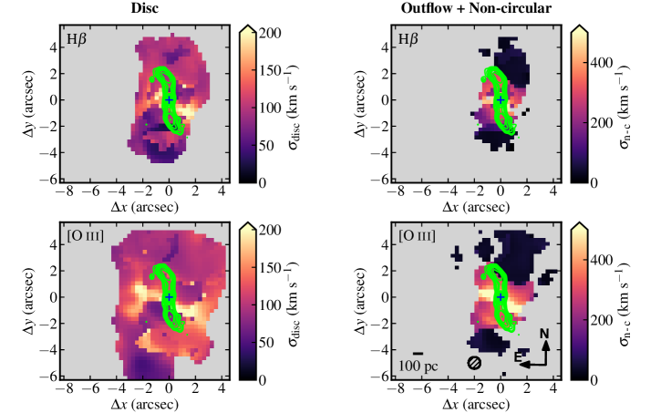
Figure 7: Velocity dispersion maps of the disc (left) and the outflow+non-circular (right) components for the lines observed with the GTC/MEGARA LR-B grating, i.e., H$\beta$ and [O III]$\lambda\lambda$4959, 5007 lines. Contours show the VLA radio jet (Sect. 2.2). Symbols as in Fig. 5.

This component classification differs from that proposed by Schnorr-Müller et al. (2014) for NGC 2110. Although for each spaxel they also fitted the emission lines in the red part of the spectrum with two components, they classified them into four categories only according to increasing velocity dispersion values, namely, outflow, warm gas disc, cold gas disc, and a north cloud. With this approach, they sought to interpret the asymmetry in the velocity field and proposed two incomplete rotating disc components (see their Figs. 5 and 6). Our kinematic classification has only one disc component, which includes a large fraction of the spaxels in their cold and warm disc components. On the other hand, we agreed with their velocity dispersion classification for the outflow component. We nevertheless found that, for the goals pursued by this work, it is sufficient to perform a classification which allows us to separate the outflow component from that of the disc and other non-circular components.

3.4 Two-dimensional maps

With the kinematics classification adopted in the previous section, we created maps of the line intensity, velocity, and velocity dispersion for the disc component and the outflow+non-circular component. For the latter, the outflow component is confined to the central $4\arcsec$ and thus is easily distinguished from the other non-circular motions by inspecting the velocity dispersion map. In Figs. 5, 6, and 7, we show the MEGARA LR-B grating maps for the intensity, velocity, and velocity dispersion, respectively for H$\beta$ and [O III]. These maps capture the most remarkable aspects of both gratings. The LR-R grating maps can be found in Appendix B.

Diagnostic diagrams (also known as BPT diagnostic diagrams) based on optical line ratios are tools to identify the dominant gas excitation mechanism in galaxies. Initially proposed by Baldwin et al. (1981) and Veilleux & Osterbrock (1987), they use a comparison of the [O III]/H$\beta$ ratio versus the [S II]/H$\alpha$, [O I]/H$\alpha$ and [N II]/H$\alpha$ ratios. These diagrams can be used to distinguish between mechanisms such as photoionisation by young stars in star forming regions, photoionisation from an AGN, or low ionisation (nuclear) emission regions (LI(N)ER). The last type is associated with the presence of shocks, as well as ionisation by hot, low-mass evolved stars (see also Sect. 4). BPT diagrams derived from IFU spectroscopy are routinely applied to local AGN (e.g., Bremer et al., 2013; Davies et al., 2016; Husemann et al., 2019; Mingozzi et al., 2019; D’Agostino et al., 2019; Smirnova-Pinchukova et al., 2019; Shimizu et al., 2019; Perna et al., 2020; Venturi et al., 2021; Comerón et al., 2021; Smirnova-Pinchukova et al., 2022; Juneau et al., 2022; Cazzoli et al., 2022). Figures 8 and 9 display the [O III]/H$\beta$ versus [N II]/H$\alpha$, [S II]/H$\alpha$, and [O I]/H$\alpha$ diagnostic diagrams, and their associated spatially-resolved maps, for the disc and outflow+non-circular components, respectively.

Finally, we computed electron density maps using the fluxes from the [S II] $\lambda\lambda$6716, 6731 doublet. In particular, we used the method Atom.getTemDen of PyNeb (Luridiana et al., 2015), and assumed a typical electron temperature of $10^{4}$ K. This method computes densities in the range 20 – 5.7 $\times$ $10^{4}$ cm^-3 for [S II]$\lambda$6731/[S II]$\lambda$6716 ratios between 0.7 and 2.2. We assigned the minimum/maximum density to those ratios which are below/above the mentioned interval. However, the upper value is only reached at one spaxel within the central region and at a spurious location of the non-circular component. The resulting electron density maps are in Fig. 10. For comparison, we also estimated the electron densities using the ionisation parameter (U) method proposed by Baron & Netzer (2019). This method only applies to gas excited by a central source (like an AGN). Given the likely mix of shock and AGN ionisation in some regions of NGC 2110 (see below), the interpretation of the electron density maps using the U method are not straightforward. The maps are shown in the Appendix in Fig. 5.

4 The disc component

The maps of the emission line fluxes for the disc component are the left panels of Figs. 5 and 19 for H$\beta$ and [O III]$\lambda$5007, and [O I]$\lambda$6300, H$\alpha$, [N II]$\lambda$6583, [S II]$\lambda$6716 and [S II]$\lambda$6731, respectively. We detected the disc component filling approximately the full MEGARA FoV along the major axis of the galaxy and approximately $8\arcsec$ along the minor axis of the galaxy. The ionised gas morphology of the disc component is dominated by the nucleus, with the extended emission tracing the disc orientation and some of the spiral morphology (marked in the bottom left panel of Fig. 5), seen in the HST image in Fig. 1 and especially in the optical color maps (see for instance, Fig. 1 of Schnorr-Müller et al., 2014).

Figures 6 and 3 (left panels) are the velocity maps of the disc component. They all show a similar structure, namely a rotation pattern in which the north half approaches the observer and the south half recedes from the observer. The absolute values of velocities in the north half are lower than those in the south half. Our results for this component are in line with the observations by Wilson & Baldwin (1985), González Delgado et al. (2002), Ferruit et al. (2004), and Rosario et al. (2010). A few spaxels close to the nucleus have high negative velocities in the maps from the [N II]$\lambda\lambda$6548, 6583 and [S II]$\lambda\lambda$6716, 6731 doublets, and correspond to spurious fits of our automatic algorithm. We also observe some discontinuities in the velocity and velocity dispersion maps, especially in transition regions between lines fitted with two components and only one component. It is possible that in some spaxels, in particular in the central and transition regions, the lines present other additional velocity components that cannot be resolved with the current spectral resolution.

Figures 8 and 9 present, for the first time, the spatially-resolved BPT diagrams of the central part of the disc and outflow region of NGC 2110. All the spaxels of the disc component fall in the AGN zone in the [N II] diagnostic diagram (Fig. 8, top left panel). There appears to be a gradient of increasing excitation to the north of the AGN location, which might also be caused by an uneven impact of the radio jet, as discussed in Sect. 3.3. LI(N)ER emission predominates in the diagnostic diagrams from [S II] and [O I] (Fig. 8, middle and bottom left panels, respectively). However, in these two last maps, there are some regions with Seyfert-like excitation, that is, gas photoionised by the AGN. These are near the AGN position as well as beyond the bending of the radio jet, both to the north and south of the AGN, at projected distances reaching at least $5\arcsec\simeq 800\,$pc. These regions appear to be coincident with the inner spiral arms marked in Fig. 5 (bottom right panel). They are likely tracing gas in the disc that is being illuminated by the AGN, as has been found in other Seyfert galaxies in the MAGNUM sample (Mingozzi et al., 2019). In fact, this morphology could be understood in the context of the geometry proposed by Rosario et al. (2010) in their Fig. 7. The Seyfert-like excitation regions could plausibly arise by the intersection of a wider-angle ionisation cone with the galaxy disc. This could also explain the relatively low ionisation of the entire observable ionisation cone, as we are only seeing the part that is on the edge of the cone due to the geometry of illumination. This region is likely to correspond to the continuation of the AGN-photoionised plume identified by Rosario et al. (2010).

Since NGC 2110 is an early-type spiral galaxy, LI(N)ER-like line ratios may not necessarily be interpreted as evidence for shocks. To rule out a dominant contribution from ionisation by evolved stars, we constructed diagrams comparing the equivalent width of H$\alpha$ (W_Hα) with the [N II]/H$\alpha$ line ratio, also known as WHAN diagrams (Cid Fernandes et al., 2010, 2011) for both the disc and outflow components. As can be seen from Fig. 11, the majority of spaxels of the disc and outflow component lie outside the region occupied by retired and passive galaxies. According to these authors, the gas excitation galaxies with very weak line emission is believed to be due to evolved stars. We can rule out that in the central disc and outflow regions of NGC 2110, the LI(N)ER-like emission is dominated by excitation from evolved stars. Therefore, considering the results from the WHAN diagrams and the seeing conditions, we can conclude that there is LI(N)ER-like excitation in galaxy regions well beyond what could be expected from beam smearing.

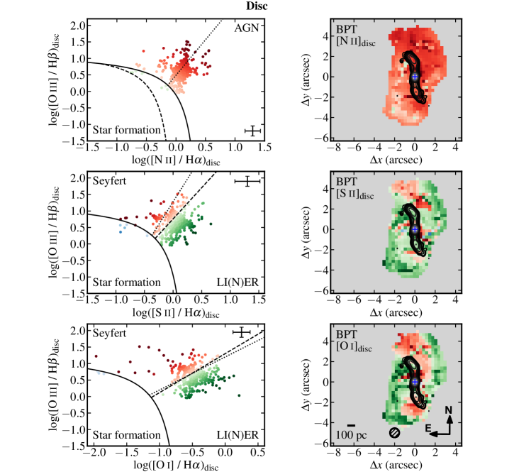
Figure 8: Spatially-resolved BPT diagnostic diagrams (left panels) and maps (right panels) for the disc component. Top, middle and bottom diagrams of the left panels correspond to [O III]$\lambda$5007/H$\beta$ versus [N II]$\lambda$6583/H$\alpha$, ([S II]$\lambda$6716 + $\lambda$6731)/H$\alpha$ and [O I]$\lambda$6300/H$\alpha$, respectively. The points in the red color scale are spaxels in the AGN/Seyfert region, those in the blue color scale are spaxels in the star-forming region, and those in the green color scale in the composite-like/LI(N)ER region. Solid curves are theoretical upper limits of starburst models from Kewley et al. (2001). The dashed curve in the [N II] diagram is the demarcation between starburst galaxies and AGN proposed by Kauffmann et al. (2003). Dashed lines in the [S II] and [O I] diagrams are classification lines proposed by Kewley et al. (2006) to split Seyfert and LI(N)ER emission. Dotted lines in the diagnostic diagrams mark bisector lines between the loci of points for the shock-excited NGC 1482 and the AGN-excited NGC 1365 (Sharp & Bland-Hawthorn, 2010). For reference, the error bars represent the measurement uncertainties in a spaxel outside the outflow region, at $\simeq 2.4\arcsec$ north of the AGN. The right panels are diagnostic maps colour coded as their corresponding diagrams to the left. Contours in maps show the radio jet using the VLA data described in Sect. 2.2.

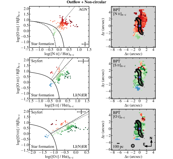
Figure 9: Spatially-resolved BPT diagnostic diagrams (left) and maps (right) for the outflow+non-circular component. All symbols, colors, and lines are as in Fig. 8.

5 The outflow component

5.1 Morphology and excitation conditions

The intensity of the outflow component of the ionised gas peaks at the AGN position (central region in the right panels of Figs. 5 and  19), and can be easily distinguished from the other non-circular motions by the velocity and velocity dispersion maps (right panels of Figs. 6,  3, 7, and  4). Nevertheless, we marked the outflow region in the bottom right panel of Fig. 5. The outflow emission is oriented along the northwest-southeast direction at a position angle that is similar to that of $-35\degr$ observed in the X-ray Fe-K$\alpha$ line by Kawamuro et al. (2020). The outflow region is clearly resolved along the north-south direction, with a projected size (FWHM) of $1.34\arcsec\simeq 214\,$pc at the [O III] wavelength compared with the measured FWHM of $0.93\arcsec$ from the calibration star at the same wavelength and direction. We obtained these measurements from the data cubes before we spatially smoothed them (see Sect. 3.1). Assuming a simple broadening in quadrature, the intrinsic size would be approximately $1\arcsec\simeq 160\,$pc (FWHM). It is just resolved in the east-west direction with a FWHM$=1.2\arcsec$, compared with the standard star size of FWHM$=0.96\arcsec$ along this direction.

The VLA radio emission (Ulvestad & Wilson, 1983) of NGC 2110 shows a collimated linear structure in an almost north-south direction in the inner $2\arcsec$. This is in agreement with the size of the outflow region. Beyond this, the radio jet bends to the northeast and southwest direction in an inverted ‘S-shaped’ morphology, which coincides with the noticeable drop observed in the MEGARA velocity dispersion maps. Within the central $\sim 2\arcsec$, the broad component flux maps (see also Ferruit et al., 2004) resolve the ‘outer plume’ (see the middle right panel of Fig. 19) detected by Rosario et al. (2010) in the HST narrow-band H$\beta$+[O III] and H$\alpha$+[N II] images, as well as some fainter spiral morphology seen on larger scales. The ‘inner plume’ identified by Rosario et al. (2010), extends only approximately $0.4\arcsec$ from the nucleus, and is not resolved in our MEGARA observations.

The outflow component shows AGN excitation in the [N II] diagnostic diagram (top right panel of Fig. 9) and a LI(N)ER excitation in the other two diagrams (middle and bottom right panels of Fig. 9), as found in other AGN (see e.g., Perna et al., 2017). The outflow component of NGC 2110 is relatively compact and does not reveal a clear conical shape illuminated by the central AGN. This contrasts with the results for the Seyfert galaxies in the MAGNUM survey (Cresci et al., 2015; Mingozzi et al., 2019) and other works (see e.g., Juneau et al., 2022), in which ionisation cones with AGN photoionised emission, with their edges showing lower ionisation, are frequently revealed in their diagnostic diagrams.

As shown above, a large fraction of the spaxels in the disc and outflow component of NGC 2110 have line ratios in the LI(N)ER region in two BPT diagrams, where the gas excitation can be explained by shocks (see Perna et al., 2017; Mingozzi et al., 2019; Cazzoli et al., 2022, and references therein) but also by X-ray radiation from the AGN and evolved stars. However, Fig. 11 (right panels) shows that most spaxels are outside the region occupied by retired and passive galaxies where the LI(N)ER excitation is produced by evolved stars. Comparing with Fig. 8 of Mingozzi et al. (2019), it would be possible to reproduce the observed line ratios for the outflow component and some regions in the disc with shock models. Such shocks might be driven by the radio jet impacting the ISM in the galaxy disc. Indeed, recent simulations show that low-power radio jets, such as those observed in Seyfert galaxies, can drive $\sim$ kpc-scale outflows, which can affect the inner galaxy disc (Mukherjee et al., 2018; Talbot et al., 2022; Meenakshi et al., 2022). The effects are especially noticeable when jets are launched at low inclinations with respect to the disc of the galaxy. Finally, we have only been able to measure all the line ratios of the non-circular component in a small number of spaxels. The north part appears to be located in the AGN area of the [N II] diagram and the LI(N)ER region in the [S II] and [O I] diagrams. The south part, at an approximate radial distance from the AGN of $\sim 4\arcsec$, appears in the composite regime and the star forming area in the BPT diagrams.

5.2 Kinematics

The velocity fields of the outflow component (central region in the right panels of Figs. 6 and 3) present moderate values of the peak velocity relative to the systemic value, typically in the $\sim 50-100\,$km s^-1 range. The typical values of the velocity dispersion in the outflow region are 700 km s^-1. The [O III]$\lambda\lambda$4959, 5007, H$\alpha$ and [N II]$\lambda\lambda$6548, 6583 maps show a linear structure almost $4\arcsec$ in size, with high blue shifts from north-east to south-west through the nucleus reaching velocities of $\sim$300 km s^-1. This region is coincident with a high-$\sigma$ strip seen in some of the outflow component velocity dispersion maps (Figs. 7 and 4) and is also seen in the disc component. It has already been reported by González Delgado et al. (2002) and Schnorr-Müller et al. (2014). This high-$\sigma$ strip is close to the minor axis of the galaxy, so it is possible that smearing of the rotation curve and other non-circular velocities could partly explain it.

The MEGARA [O III]$\lambda$5007 position-velocity (p-v) diagrams along the major and minor axis of the galaxy (Fig. 12) are useful to identify the velocities of the outflow. We constructed these diagrams from the LR-B data cube after continuum subtraction and using an aperture of $0.9\arcsec$. The diagram for the major axis can be compared with that presented by Rosario et al. (2010) for their HST slit-A spectroscopy (c.f. their Fig. 3). We note that the PA of their slit is not exactly along the major axis of the galaxy, but it is close enough for this comparison. As can be seen from left panel of Fig. 12, the MEGARA p-v diagram reproduces well the HST observations considering our $\sim 0.9\arcsec$ seeing conditions. This p-v diagram also reveals the asymmetric rotation curve discussed in Sect. 3.3. To the southeast of the AGN, at distances of $\simeq 2.5\arcsec$, it clearly shows the two velocity components fitted in Fig. 4. The outflow can be seen as much higher velocities in the central $\simeq 2\arcsec$, both blueshifted to velocities in excess of $-1000\,\mathrm{km\,s}^{-1}$ and redshifted to velocities of several hundreds of km s^-1. The largest values of the blueshifted velocities are mostly concentrated in the nuclear region while some more moderate redshifted and blueshifted velocities are observed along the major axis to the northwest of the AGN.

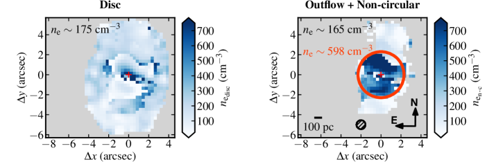
Figure 10: Maps of electron densities for the disc (left) and the outflow+non-circular (right) components using the [S II] doublet ratio method. Values on top left corners indicate the median density in each map.

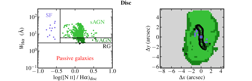
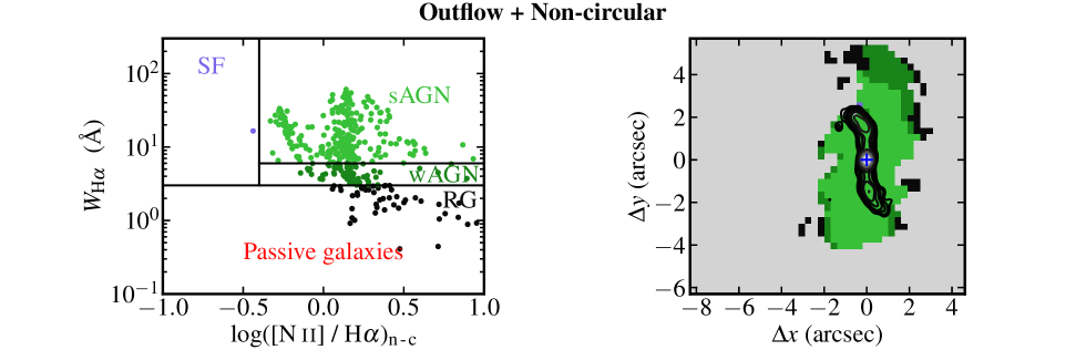
Figure 11: WHAN diagrams (left panels) for the disc component (top) and for the outflow and non-circular motion components (bottom) and the corresponding spatial distribution of the WHAN regions (right panels). See Cid Fernandes et al. (2011) for details for the different region definitions. SF: star forming galaxies, sAGN: strong AGN, wAGN: weak AGN, and RG: retired galaxies.

Along the galaxy minor axis, the MEGARA p-v diagram shows at the nuclear position a broad range of velocities, both redshifted and blueshifted velocities, with the latter reaching maximum outflow velocities in excess of $\simeq-1000\,\mathrm{km\,s}^{-1}$ at the AGN position. We note that in the blue part of the spectrum in the p-v diagrams the two [O III] lines start mixing as they are about $2870\,\mathrm{km\,s}^{-1}$ apart. Nevertheless, the observed high velocities are beyond the range of velocities attributable to any possible effect of smearing of rotation curve at the AGN position $(\simeq 400\,\mathrm{km\,s}^{-1}$). The large blueshifts observed along both axes can be associated with the broadest of the three components fitted for the nuclear spectrum (see Table 2 and Fig. 2), with $\sigma=662\,\mathrm{km\,s}^{-1}$. Finally, there is [O III] emission in the two quadrants forbidden by disc rotation along the major axis p-v diagram. They show velocities of a few hundred km s^-1, seen as redshifted motions to the northwest and blueshifted motions to the southeast. If we assumed these motions are in the plane of the galaxy, they would imply counter-rotation. However, given the velocities and velocity dispersions fitted in the outflow region, it is more reasonable to assume that they trace outflowing gas outside the plane of the galaxy in NGC 2110.

5.3 Electron densities

Figure 10 shows the electron density maps for each of the two kinematic components using the [S II] method. The outflow region presents a median value of $n_{\mathrm{e}}\sim$600 cm^-3, which is considerably higher than the values of the non-circular motions and the disc. The latter has a median value of $\sim$175 cm^-3. Analogous to our work, Kakkad et al. (2018) studied the spatial distribution of electron density for the outflow component of NGC 2110 (their Fig. 9). Although the comparison is not straightforward, mainly due to their poorer seeing conditions, they found the same tendency of higher values within the outflow region and smaller values for higher distances of this component.

Davies et al. (2020) estimated the electron density for an aperture of $1.8\arcsec\times 1.8\arcsec$ around the nucleus with three different methods without splitting the flux in different kinematic components. In particular, they found a value of 350 cm^-3 from the [S II] doublet. This is in the middle of our estimations for the two components, indicating a good agreement with those authors. We note, however, that with the ionisation parameter method they derived values of the electron density of up to 43000 cm^-3, in agreement with our estimates using the same method (see the electron density maps in Fig. 5).

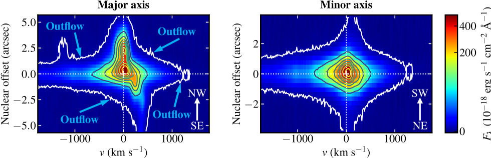
Figure 12: GTC/MEGARA p-v diagrams extracted for the [O III]$\lambda$5007 line after continuum subtraction, along the major (PA=$163^{\circ}$, left panel) and minor (PA=$73^{\circ}$, right panel) axes of NGC 2110. The first contour is plotted at three times the noise at approximately 1350 km s^-1. The second contour is at five times the noise, reaching velocities of $-650/500\,\mathrm{km\,s}^{-1}$, and the rest of the contours are on a linear scale.

5.4 Outflow properties

In this section, we compute the outflow properties using the [O III] line, as in Davies et al. (2020), to allow for a comparison with their work. In the next section, we also estimate some outflow properties using H$\alpha$. Before we estimated the outflowing gas mass from the [O III] luminosity (see below), we computed the extinction in the outflow region, using the integrated H$\alpha$ and H$\beta$ fluxes. We made use of the extinction law from Cardelli et al. (1989) with a parameter $R_{V}=3.1$, assuming an intrinsic ratio between the Balmer lines of H$\alpha$ and H$\beta$ of 3.1. We then used the derived extinction to correct the observed [O III] flux. Our median extinction value ($A_{V}=0.82\,$mag) over the outflow region is lower than the values reported by Davies et al. (2020) and Thomas et al. (2017), which are 1.7 and 2.4 mag, respectively. Apart from the different physical sizes used for the spectra extraction, we also checked whether the differences are mainly due to the fact that these works did not split the flux in kinematic components for their estimations. Interestingly, we derived an extinction of $A_{V}=2.0\,$mag for the disc component for an aperture as that of Davies et al. (2020). Thus, this may explain thus the differences. Nevertheless, we corrected the [O III] fluxes within the outflow region with the corresponding median value of the extinction.

Considering equation B3 of Fiore et al. (2017), the mass of ionised gas based on the [O III] luminosity can be expressed as (see also Carniani et al., 2015):

$$M^{[{O\textsc{III}}]}=4.0\times 10^{7}\mathrm{M_{\odot}}\frac{C}{10^{\mathrm{[O/H]}}}\frac{L^{[{O\textsc{III}}]}}{10^{44}\ \mathrm{erg\ s^{-1}}}\frac{1000\ \mathrm{cm^{-3}}}{n_{\mathrm{e}}},$$ (1)

where $C$ is the condensation factor and [O/H] the oxygen abundance ratio (i.e., the ratio of AGN oxygen abundance compared to that of the Sun on a logarithmic scale), we derived an [O III] mass map. For simplicity, we assumed that the gas clouds have the same electron density, leading to a value of $C=1$. $A(\mathrm{X})$ is the elemental abundance expressed as the logarithm of the number of atoms of an element X per $10^{12}$ atoms of hydrogen. The oxygen abundance ratio is related to a AGN oxygen abundance and that of the Sun as follows: $\mathrm{[O/H]}=A(\mathrm{O})-A(\mathrm{O})_{\odot}$, where the required oxygen abundances for NGC 2110 and the Sun are known from the literature: $A(\mathrm{O})=8.87$ (Dors et al., 2015) and $A(\mathrm{O})_{\odot}=8.86$ (Centeno & Socas-Navarro, 2008).

Finally, for estimating the total outflowing mass of ionised gas $M$ in each spaxel (using the corresponding value of the electron density), we used the approximation adopted by Fiore et al. (2017) in terms of the [O III] outflowing mass:

$$M_{\rm out}=3\times M^{[{O\textsc{III}}]}.$$ (2)

We obtained an ionised mass in the outflow of $9.8\times 10^{4}\,M_{\odot}$. We note that in the following section we provide another estimate of the outflowing mass of ionised gas using H$\alpha$ measurements.

For the NGC 2110 outflow it seems reasonable to adopt a constant outflow history through a cone/sphere to the outflow properties (see Lutz et al., 2020). This assumption leads to the following equations for the mass outflow rate $\dot{M}_{\mathrm{out}}$, the kinetic energy $E_{\mathrm{kin}}$, the kinetic power $\dot{E}_{\mathrm{kin}}$ and the momentum rate $\dot{P}$:

$$\dot{M}_{\mathrm{out}} = M_{\mathrm{out}}\frac{v_{\mathrm{out}}}{r_{\mathrm{out}}}$$ (3)

$$E_{\mathrm{kin}} = \frac{1}{2}M_{\mathrm{out}}v_{\mathrm{out}}^{2}$$ (4)

$$\dot{E}_{\mathrm{kin}} = \frac{1}{2}\dot{M}_{\mathrm{out}}v_{\mathrm{out}}^{2}$$ (5)

$$\dot{P} = \dot{M}_{\mathrm{out}}v_{\mathrm{out}}$$ (6)

where $M_{\mathrm{out}}$ is the ionised gas mass integrated within the outflow region, $v_{\mathrm{out}}$ the outflow velocity, and $r_{\mathrm{out}}$ the outflow radius.

In order to estimate the outflow velocity $v_{\mathrm{out}}$, we used a similar approach to that of Davies et al. (2020). We computed the percentiles 2 and 98 of the velocity distribution inferred from the outflow profile of the [O III] doublet, measured their differences with respect to the systemic velocity, and chose whichever is larger. We obtained a maximum outflowing velocity of $v_{98}=1167\,\mathrm{km\,s}^{-1}$, whereas they reported a value of $1665\,\mathrm{km\,s}^{-1}$. We note that apart from the different extraction sizes, they assumed that the whole profile is dominated by the outflow, while we built the outflow profile stacking the line profiles of the non-circular component in each spaxel within the outflow region. As a note, our kinematic decomposition allowed us to estimate that approximately half of the flux of the whole profile in the $\sim 4\arcsec$ region comes from the disc component.

For the outflow radius we took $r_{\mathrm{out}}=400\ \mathrm{pc}$ (projected value, see Fig. 5), which is 2.7 times larger than the value adopted by Davies et al. (2020). The outflow region size is approximately consistent with two times the measured FWHM at the wavelength of [O III] (see Sect. 5.1). We also checked that our estimation is equivalent to that employed by Kang & Woo (2018), who defined the outflow radius as the distance in which the velocity dispersion from the [O III] doublet changes with respect to the stellar values. Indeed, the observed velocity dispersions in the outflow region of NGC 2110 (see e.g., Fig. 7) are higher than the stellar velocity dispersion ($220-260\,$km s^-1, see Nelson & Whittle, 1995; González Delgado et al., 2002; Burtscher et al., 2021). However, the measured radius for NGC 2110 falls approximately 4$\sigma$ below the expected value from the correlation between the outflow size and [O III] luminosity reported by Kang & Woo (2018) for more luminous AGN. Table 3 summarises the properties of the outflow.

Table 3: Outflow properties from the [O III] line.

Property	Value
$M_{\mathrm{out}}\ (\mathrm{M_{\odot}})$	$9.8\times 10^{4}$
$\dot{M}_{\mathrm{out}}\ (\mathrm{M_{\odot}\ yr^{-1}})$	$0.29$
$E_{\mathrm{kin}}\ (\mathrm{erg})$	$1.3\times 10^{54}$
$\dot{E}_{\mathrm{kin}}\ (\mathrm{erg\ s^{-1}})$	$1.3\times 10^{41}$
$\dot{P}\ (\mathrm{dyn})$	$2.2\times 10^{33}$

Davies et al. (2020) also computed the outflow properties of NGC 2110 and derived a mass outflow rate that is approximately an order magnitude lower. Their $L^{[{O\textsc{III}}]}$ is 0.12 dex lower than ours. Their lower flux calibration (by 0.40 dex, see Sect. 2.1) is compensated with their extinction correction, which is 0.39 dex higher. Therefore, the difference in luminosity is due to their light loss caused by their smaller aperture (0.20 dex), even though they assumed that all the light can be attributed to the outflow. Regarding $M_{\mathrm{out}}$, they obtained a value 1.59 dex lower, which is mainly due to their much higher value of the electron density. For the ionised gas mass rate $\dot{M}_{\mathrm{out}}$, the difference decreases to 0.99 dex because we considered an outflowing velocity 0.15 dex lower and a radius 0.43 higher (which in both cases help to alleviate the difference). The same happens for the kinetic power $\dot{E}_{\mathrm{kin}}$. All this highlights the importance of understanding the assumptions for estimating the outflow properties while comparing with results from other works.

5.5 Are the outflow properties linked with the radio jet?

NGC 2110 follows well the scaling relation of the ionised mass outflow rate and the AGN bolometric luminosity derived by Fiore et al. (2017) for luminous AGN using $\log L_{\mathrm{AGN}}=44.5\,\mathrm{erg\,s}^{-1}$ from Davies et al. (2020). However, it falls below the scaling relation with the kinetic power. In this respect, NGC 2110 behaves like other AGN of similar luminosities (see e.g., Fig. 10 of García-Bernete et al., 2021), which show a large range of kinetic powers. Moreover, NGC 2110 lies in the upper envelop of this observed large scatter at a given AGN luminosity. It is possible that, at least in cases such as NGC 2110, some of the kinetic power, in addition to that provided by the AGN radiation pressure, might be due to the effect of a moderate power radio jet. In this section we explore this scenario in NGC 2110.

Venturi et al. (2021) observed in a small sample of Seyfert galaxies that regions with high velocity dispersion were generally perpendicular to the orientation of the radio jet. In NGC 2110, the increased velocity dispersions, compared to those of the disc, are observed both perpendicular and parallel to the radio jet. Equally conspicuous is the fact that the bending of the radio jet, to the northeast and southwest within the outflow region of NGC 2110, coincides with the sharp transition in velocity dispersions seen in the region with the non-circular motions (right panels of Figs. 7 and 4). The length of the linear part of the radio jet nearly matches that of the outflow region. In this this region, there is also weak CO(2-1) emission, termed the ”lacuna”, along the northwest-southeast direction (PA$\simeq-25^{\circ}$) passing through the AGN location (Rosario et al., 2019). In this section, we investigate whether the outflow properties of NGC 2110 follow the relations between the jet radio power and the outflowing ionised mass and kinetic energy found by Venturi et al. (2021).

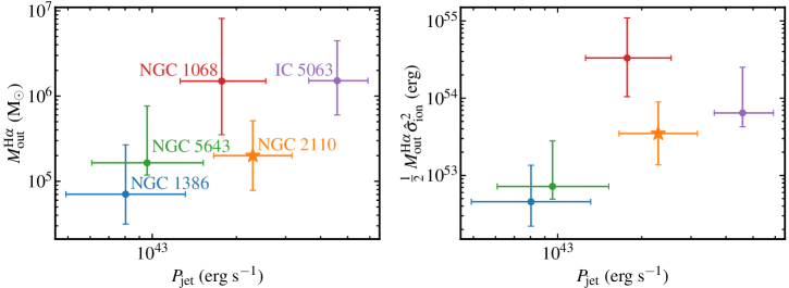
Figure 13: Outflow mass (left panel) and a proxy for the kinetic energy (right panel) versus the jet radio power. Circles are galaxies from Venturi et al. (2021), while the star corresponds to NGC 2110 (see Sect. 5.5). For this galaxy, the outflowing ionised gas mass corresponds only to that observed in the outflow region. The horizontal error bars for NGC 2110 take into account the errors in equation 16 of Bîrzan et al. (2008), while vertical error bars include the uncertainties related to the extinction correction and the relative flux calibration between the two MEGARA gratings, as well as the uncertainty from the absolute flux calibration.

We estimated the kinetic power of the radio jet for NGC 2110 from the 20 cm radio flux reported by Nagar et al. (1999). We converted the total radio flux into kinetic power using equation 16 of Bîrzan et al. (2008), as done by Venturi et al. (2021). We note, however, that other calibrations might provide kinetic powers differing by up to an order of magnitude. We obtained $P_{\mathrm{jet}}=2.3\times 10^{43}\ \mathrm{erg\,s^{-1}}$ for NGC 2110, which is slightly higher than that of NGC 1068 and approximately a factor of two less powerful than the jet in IC 5063 (Venturi et al., 2021).

To make a proper comparison with Venturi et al. (2021), we estimated the outflowing mass with our extinction corrected H$\alpha$ luminosity and their equation 1, instead of our equations 1 and 2. Unlike their work, for NGC 2110 we only included the mass from the outflow component. With this approach, the outflowing ionised mass within the outflow region is $M_{\mathrm{out}}^{\mathrm{H\alpha}}=2.0\times 10^{5}\mathrm{M_{\odot}}$, which is a factor of two higher than our value estimated from the [O III] line (Table 3). Finally, we would like to emphasise that our mass estimates and theirs are based on electron densities from the [S II] method. Following Venturi et al. (2021), the kinetic energy of the jet is $M_{\mathrm{out}}\hat{\sigma}_{\mathrm{ion}}^{2}/2$. We measured the velocity dispersion of the [O III] profile including both components, as in their work, that is from its second-order moment. We obtained $\hat{\sigma}_{\mathrm{ion}}$=419 km s^-1.

In Fig. 13 we compare NGC 2110 with the trends observed by Venturi et al. (2021) between the outflow properties and the jet radio power. NGC 2110 appears to follow well the trends suggested by their galaxies, except for the more extreme properties of NGC 1068. The derived kinetic energy in NGC 2110 is between NGC 5643 and IC 5063, which are well-known for hosting a radio jet that is close to the disc of the galaxy and driving a multi-phase energetic outflow (see Morganti et al., 2015; Venturi et al., 2021, and references therein). On the other hand, in these diagrams NGC 1068 is well above the trends. As in NGC 2110, the radio jet of NGC 1068 suffers a reorientation due probably to the impact with a gas cloud in the disc of the galaxy, and further away (a few hundred pc from the AGN) the radio morphology resembles a bow-shock (García-Burillo et al., 2014, 2017). However unlike NGC 2110, in NGC 1068 shocks only dominate the gas excitation at the radio jet location, while AGN and star formation excitation dominate in other regions (D’Agostino et al., 2019).

Considering the above observational evidence, we speculate that the radio jet propagated through the nuclear region of NGC 2110 and shocked the gas producing highly turbulent motions, both parallel and perpendicular to the radio jet. Indeed, Ulvestad & Wilson (1983) proposed that that the radio jet morphology of NGC 2110 is due to ram pressure bending by a dense rotating disc. Simulations predict that the gas would expand like a bubble (e.g., Wagner & Bicknell, 2011; Mukherjee et al., 2018). Since in NGC 2110 the jet is not perpendicular to the galaxy disc (Pringle et al., 1999), the jet-inflated bubble probably ended up impacting the ISM of the galaxy disc. As a result the jet was deflected and probably decelerated. This may have caused a decrease in the turbulence of the gas, and thus lower observed velocity dispersions in the non-circular component outside the outflow region. In the disc of the galaxy we observe shock-like emission in the central region where the jet is still operating but at distances beyond the radio bend the dominance of shocks diminishes and it is then possible to identify gas excited by the AGN (see Fig 8).

In summary, the discussion above provides additional support for the scenario where part of the observed ionised gas outflow in NGC 2110 could be driven by the radio jet when it expands laterally and radially in the disc of the galaxy.

6 Summary and conclusions

In this paper, we presented new GTC/MEGARA IFU observations of the central $\sim 13\arcsec\times 11\arcsec$ ($\sim 2\,\mathrm{kpc}\times 1.8\,\mathrm{kpc}$ in projection) region of NGC 2110 with $R\simeq 5000-5900$. We used two gratings to observe the most prominent nebular emission lines in the $4300-5200\,\AA$ and $6100-7300\,\AA$ spectral ranges. The goal was to study the spatially-resolved properties of the ionised gas in the central 2 kpc of NGC 2110, including its outflow, and evaluate the role of its radio jet. We fitted the emission lines with a maximum of two Gaussian components, which was sufficient in the majority of spaxels, except at the AGN position. We performed a kinematic separation using the observed velocities and velocity dispersions and a comparison with the stellar kinematics from González Delgado et al. (2002) and Ferruit et al. (2004).

We identified the ionised gas rotation in the disc of the galaxy with an intermediate velocity dispersion component ($\sigma\simeq 60-200\,\mathrm{km\,s}^{-1}$). It is detected in all the bright emission lines ([O III], H$\alpha$, [N II] and [S II]) over a $\sim 8\arcsec\times 12\arcsec$ ($1.3\times 1.9$ kpc² in projection), which corresponds to most of the MEGARA FoV along the major axis of the galaxy.

The non-circular component covers a $\sim 4\arcsec\times 8\arcsec$ area and presents different properties in two distinct regions. The first is a spatially-resolved region, mostly in the north-south direction, with a total size of $\sim 2.5\arcsec\sim 400\,$pc around the nucleus. It presents the highest velocity dispersions, typically 700 km s^-1, and is identified with the ionised outflow in this galaxy. The extent of the outflow region, as traced by the [O III] line, is approximately equal to the linear part of the radio jet. Outside the outflow region, beyond the edges of the radio source and where it is deflected, the kinematics of the gas with non-circular motions changes drastically. The velocity dispersion drops to $<60\,$km s^-1. These are likely non- circular motions taking place in the disc of the galaxy, possibly unrelated to the inner outflow and the radio jet.

We fitted the AGN nuclear spectrum of NGC 2110 with three Gaussian components, with the broadest [O III] component reaching a velocity dispersion of 662 km s^-1. The [O III] p-v diagrams along the major and minor axes of the galaxy reveal at the AGN position observed velocities in excess of $1000\,\mathrm{km\,s}^{-1}$, both blueshifted and redshifted. There are other redshifted and blueshifted components of several hundreds of km s^-1 in the p-v diagram along the major axis of the galaxy. Their location in the two quadrants forbidden by rotation indicates that part of the outflowing gas is outside the disc of the galaxy.

The spatially-resolved BPT diagnostic diagrams of the outflow region reveal mostly LI(N)ER-like excitation. The observed line ratios are consistent with predictions from shock models. In the disc of the galaxy, there is a large number of spaxels with LI(N)ER-like excitation, but also ‘Seyfert-like’ excitation due to AGN photoionisation. The latter excitation appears in regions beyond, although close to, the region where the radio jet is bent, at projected distances greater than approximately $1-2\arcsec$, reaching at least $5\arcsec\simeq 800\,$pc. This is likely gas in the host galaxy disc being illuminated by AGN photons at the intersection of a ionisation cone with the galaxy disc (see also Rosario et al., 2010).

Using the outflow component of the [O III]$\lambda$5007 line, we derived an outflowing ionised gas mass, ionised mass outflow rate, and outflow kinetic power of $M_{\mathrm{out}}=9.8\times 10^{4}\ \mathrm{M_{\odot}}$, $\dot{M}_{\mathrm{out}}=0.29\ \mathrm{M_{\odot}\ yr^{-1}}$ and $\dot{E}_{\mathrm{kin}}=1.3\times 10^{41}\ \mathrm{erg\ s^{-1}}$, respectively. As found in other Seyfert galaxies, NGC 2110 lies below the correlation between the AGN bolometric luminosity and kinetic power of the ionised outflow derived for luminous AGN. However, NGC 2110 shows an increased kinetic power when compared to other Seyferts of similar AGN luminosity. We explored the possibility that part of the kinetic power might be due to the effect of the moderate power radio jet detected in this galaxy. To do so, we compared NGC 2110 outflowing gas mass and kinetic power properties with its jet radio power. NGC 2110 follows well the observational trends between these quantities found by Venturi et al. (2021) for a few Seyfert galaxies. We proposed that the ionised gas outflow in the inner $\simeq 400\,$pc region of NGC 2110 is driven in part by the radio jet. This is supported by the presence of shock-like emission, presumably induced by the passage of the moderate luminosity radio jet through the disc. However, beyond the outflow region there is also gas photoionised by the AGN in the central 2 kpc of NGC 2110. This gas is rotating and located in regions bordering and past the radio jet beding, where it is being illuminated by AGN photons.

Appendix A MEGARA fits with three components for the nuclear region

Figs. 14, 15, 16, and 17 display the spectra from 3-spaxel square extractions in the nuclear region and their fits with three components, like Fig. 2 which shows the spectral region around the [O III]$\lambda\lambda$4959, 5007 doublet in the main text. The physical parameters of these fits are provided in Table 2.

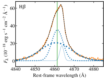
Figure 14: Spectrum of the H$\beta$ line extracted in the nuclear region fitted with 3 components. All lines are as in Fig. 2.

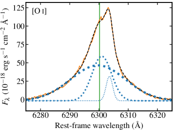
Figure 15: Spectrum of the [O I]$\lambda$6300 line extracted in the nuclear region fitted with 3 components. All lines are as in Fig. 2.

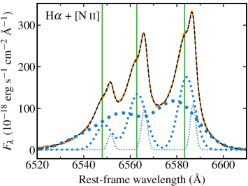
Figure 16: Spectrum of the H$\alpha$ line and the [N II]$\lambda\lambda$6548, 6583 doublet extracted in the nuclear region fitted with 3 components. All lines are as in Fig. 2.

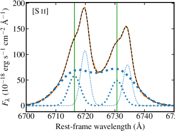
Figure 17: Spectrum of the [S II] $\lambda\lambda$6716, 6731 doublet extracted in the nuclear region fitted with 3 components. All lines are as in Fig. 2.

Appendix B Figures for the emission lines observed with the MEGARA LR-R grating

In this Appendix, Figs. 18, 19, 3, and 4 show the same information as Figs. 3, 5, 6, and 7 but for the emission-lines in the MEGARA LR-R grating.

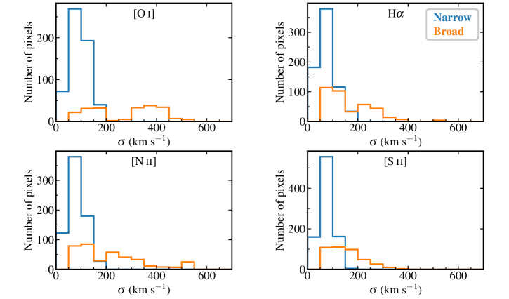
Figure 18: Distributions of the velocity dispersion (corrected for instrumental resolution) measured on a spaxel-by-spaxel basis of the fits using a maximum of two Gaussian components from lines observed with the MEGARA LR-R grating, i.e., [O I]$\lambda$6300, H$\alpha$, [N II]$\lambda\lambda$6548, 6583 and [S II]$\lambda\lambda$6716, 6731 lines. Same as in Fig. 3.

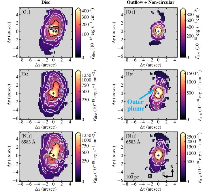
Figure 19: Flux maps of the disc and outflow+non-circular components for lines observed with the MEGARA LR-R grating, i.e., [O I]$\lambda$6300, H$\alpha$, [N II]$\lambda$6583, [S II]$\lambda$6716 and [S II] $\lambda$6731 lines. Contour definition and symbols are as in Fig. 5.

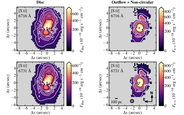
Figure 2: continued.

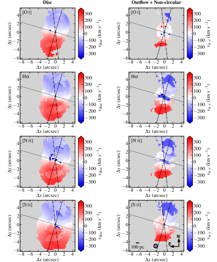
Figure 3: Velocity maps of the disc and outflow+non-circular components for lines observed with the MEGARA LR-R grating, i.e., [O I]$\lambda$6300, H$\alpha$, [N II]$\lambda\lambda$6548, 6583 and [S II]$\lambda\lambda$6716, 6731 lines. Same as in Fig. 6.

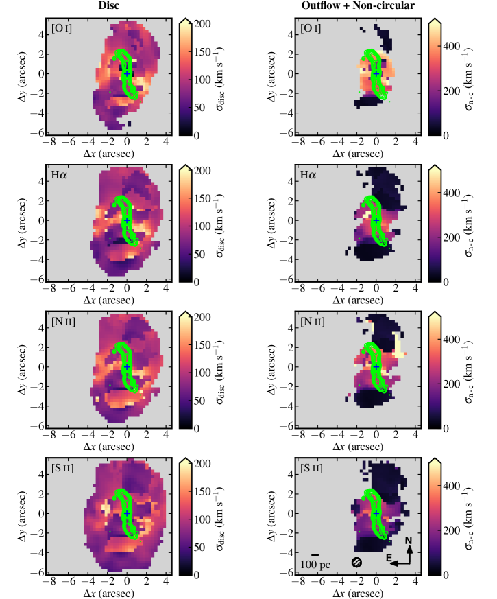
Figure 4: Velocity-dispersion maps of the disc and outflow+non-circular components for lines observed with the MEGARA LR-R grating, i.e., [O I]$\lambda$6300, H$\alpha$, [N II]$\lambda\lambda$6548, 6583 and [S II]$\lambda\lambda$6716, 6731 lines. Same as in Fig. 7.

Appendix C Electron densities from the ionisation parameter method

In this Appendix, Fig. 5 shows the estimation of the electron densities using the ionisation parameter method proposed by Baron & Netzer (2019). See the main text for details and caveats related to this method.

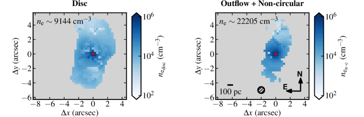
Figure 5: Maps of electron densities for the disc (left) and outflow+non-circular (right) components using the ionisation parameter method (see text for details).