An Overview of Asymptotic Normality in Stochastic Blockmodels: Cluster Analysis and Inference
Abstract
This paper provides a selective review of the statistical network analysis literature focused on clustering and inference problems for stochastic blockmodels and their variants. We survey asymptotic normality results for stochastic blockmodels as a means of thematically linking classical statistical concepts to contemporary research in network data analysis. Of note, multiple different forms of asymptotically Gaussian behavior arise in stochastic blockmodels and are useful for different purposes, pertaining to estimation and testing, the characterization of cluster structure in community detection, and understanding latent space geometry. This paper concludes with a discussion of open problems and ongoing research activities addressing asymptotic normality and its implications for statistical network modeling.
1 Introduction
Stochastic blockmodels (SBMs) ((Wasserman and Faust, 1994; Holland et al., 1983) are generative models for random graphs that posit community structure among nodes, manifest as block-structured connectivity patterns. In the simplest setting, nodes (vertices) belong to communities, and connectivity, as quantified via the presence or absence of links (edges) between nodes, is probabilistically governed solely by nodes’ community memberships. Stochastic blockmodels and their variants serve as workhorse generative models in the statistical analysis of networks, particularly in the vertex-centric, networks-as-graphs paradigm. Broadly speaking, this is due largely to the fact that SBMs simultaneously provide enough heterogeneity and enough homogeneity in the sense that (i) SBMs are structured enough to be statistically interesting, serving as a stepping stone for eventual real data considerations, and (ii) SBMs are tractable enough to enable theoretical analysis of estimation methods and computational procedures.
Stochastic blockmodels, instances of which are sometimes referred to as ‘planted partition models’ ((Schaeffer, 2007; Lancichinetti and Fortunato, 2009), have received significant attention within the mathematics, statistics, computer science, and physics research communities, finding applications in social network analysis, neuroimaging, and elsewhere. Popular variants and extensions include mixed membership ((Airoldi et al., 2008) and degree-corrected stochastic blockmodels ((Karrer and Newman, 2011), among numerous others ((Arroyo and Levina, 2022; Zhang et al., 2020; Sengupta and Chen, 2018; Noroozi et al., 2021b, a).
Historical developments in the study of networks and on the role of SBMs are cataloged in, for example, Fortunato ((2010); Goldenberg et al. ((2009); Fortunato and Hric ((2016); Lee and Wilkinson ((2019); Wasserman and Faust ((1994). Stochastic blockmodels have themselves already been the subject of survey-length treatment, notably Abbe ((2018) which summarizes phase transition phenomena and algorithmic considerations under various mathematical regimes. Stochastic blockmodels also arise in survey-length treatments of network-oriented research focused on dynamic networks ((Kim et al., 2018) as well as latent space modeling and analysis ((Athreya et al., 2018; Matias and Robin, 2014), among others ((Gao and Ma, 2021; Goldenberg et al., 2009; Zhao, 2017).
The study of networks at times challenges convention and intuition developed in standard statistical training, as single-network realizations constitute a single “observation”. Namely, one might observe a single network describing pairwise interactions between vertices, in contrast to observing independent Euclidean-valued feature vectors. In the context of modeling network data, several natural questions arise. One might ask: where or how could asymptotic normality appear, and to what end? Possible answers depend on how statistical units of interest are conceptualized. Further questions might include: do multiple networks (graphs) constitute multiple units/observations, or are individual vertices within a single network the units of interest? Correspondingly, is the inference task focused on vertex-specific behavior by, for example, seeking to infer individual edge probability parameters, or does one wish to understand the behavior of specified summary statistics computed from the entire network? This survey contributes to the existing literature by providing a unified treatment of numerous asymptotic normality results for stochastic blockmodels, as a means of contextualizing and detailing the statistical aspects of advances in statistical network analysis.
A sizeable body of literature considers nonparametric spectral-based matrix factorization approaches to network analysis, leveraging the convenient representation of networks in terms of their adjacency or Laplacian matrix. This has led to widespread use of spectral embeddings, namely eigendecomposition-based low-dimensional Euclidean representations of vertices in graphs. This survey considers existing asymptotic normality results for different matrix factorization approaches to network analysis as well as applications of these results to parameter estimation and hypothesis testing. In part, this survey seeks to elucidate, to the extent possible, the interplay between underlying matrix structure and the associated asymptotic normality. Loosely speaking, a tug-of-war exists between network sparsity (the antagonist) and network (sample) size (the protagonist). The emergence of asymptotic normality depends on the extent of community separation (between-community heterogeneity), sample size, and sparsity, with rate of convergence, covariance matrix, and centering determined by these three factors.
Numerous existing works in the literature address statistical consistency under SBMs and in more general network settings, without addressing asymptotic distributional properties. To maintain focus and a reasonable page count, this survey restricts its attention to only the most closely related works. In particular, this review does not delve into the rich literature on information-theoretical thresholds and phase transition phenomena for random graphs ((Abbe, 2018), nor does it consider graphons as graph limit objects ((Lovász, 2012). Many of the results covered hold for more general models, and, where appropriate, we mention when such results hold, though presentation herein is deliberately restricted to stochastic blockmodels.
1.1 Notation
For any positive integer , define . We write to denote that the random variable is distributed according to the distribution . We use lowercase letters to denote vectors, writing the vector coordinate-wise as . We use both as a scalar and to denote the vector of all ones when its dimension is clear from context. We write to denote the interior of the unit simplex in dimensions, i.e., if and only if simultaneously and entrywise for each . We use upper case letters to denote matrices, say , where and denote the -th row and -th column of , respectively. We use for the largest singular value of and for the Frobenius matrix norm. We use uppercase letters to denote random vectors, with single indices corresponding to individual observables.
We use the asymptotic notation when there exists a constant such that holds for all sufficiently large. Similarly, indicates that simultaneously and , whereas denotes as . In addition, we write if and if , and if . Finally, we write when there exists a constant not depending on such that .
2 Stochastic Blockmodels
This section briefly reviews the basics of stochastic blockmodeling wherein graphs or networks constitute observed data. Arising at the confluence of ‘blockmodeling’ and ‘stochastic modeling’, (directed) SBMs date back several decades Holland et al. ((1983); Wasserman and Faust ((1994). Significant attention has been paid to SBMs as concrete instances of more general latent space network models ((Hoff et al., 2002).
Definition 1 (Stochastic blockmodel – undirected, hollow).
Let be a symmetric connectivity matrix, let , and let . We say is the adjacency matrix for a stochastic blockmodel graph with sparsity factor if the block assignment map satisfies for each , and, conditional on , the upper triangular entries are independently generated in the manner
In words, vertex belongs to community with probability , and conditional on the community memberships, the probability of an edge occurring between two vertices is determined solely by the community memberships.
Remark 1 (Presence or absence of loops).
In the definition above, self-edges (loops) are not permitted (i.e., hollowness is enforced), since for all . If instead self-edges are permitted (i.e., hollowness is not enforced), then the main diagonal entries are often taken to be independent random variables with for all .
Remark 2 (Fixed community memberships and the expected adjacency matrix).
When the community memberships are taken to be fixed (nonrandom), the matrix of edge probabilities for generating an adjacency matrix , denoted by , can be expressed as provided the matrix satisfies if and only if . Depending on whether or not the graph corresponding to is permitted to have self-edges, per Definition 1, either or . In certain instances, the distinction between allowing or forbidding the presence of self-edges has a negligible impact on statistical performance guarantees and procedures, while at other times the distinction cannot be ignored. The latter point is addressed further in subsequent sections when important.
Throughout this work we will assume that has distinct rows. This specification prevents multiple communities from exhibiting identical, indistinguishable connectivity behavior, thereby mitigating a potential source of model non-identifiability.
2.1 Generalizations of Blockmodels
The standard stochastic blockmodel permits heterogeneous nodal connectivity across different blocks (communities) but simultaneously imposes stochastic equivalence on all nodes belonging to the same block. In other words, vertices in a SBM graph can be viewed as each possessing a single, latent attribute that governs edge formation. A more flexible and arguably realistic modeling approach would allow vertices to possess shared characteristics, to various extents, from amongst a common set of possible characteristics. Enter the mixed-membership stochastic blockmodel (MMSBM) ((Airoldi et al., 2008).
Definition 2 (Mixed-membership stochastic blockmodel — undirected, loopy).
We say is the adjacency matrix for a mixed-membership stochastic blockmodel graph on vertices with sparsity factor when the upper triangular entries are independently generated in the manner
where is a symmetric connectivity matrix and is a collection of non-negative mixed membership vectors satisfying . The unobserved vectors could be specified as deterministic or could be modeled in a generative fashion, for example i.i.d. for some concentration parameter vector .
The MMSBM reduces to the SBM when all nodes in the graph are pure nodes, namely when their mixed membership vectors are all standard basis vectors. A different approach to generalizing SBMs is to permit further node-specific connectivity properties, modeled by permitting heterogeneous vertex degrees and interpretable as a measure of ‘importance’ in a network, at the expense of introducing additional parameters and model complexity. Thus arises the degree-corrected stochastic blockmodel (DCSBM) ((Karrer and Newman, 2011; Dasgupta et al., 2004).
Definition 3 (Degree-corrected stochastic blockmodel — undirected, hollow).
We say is an adjacency matrix for a degree-corrected stochastic blockmodel graph on vertices with sparsity factor when the upper triangular entries are independently generated in the manner
where is a symmetric connectivity matrix, is a nonnegative vector of node-specific degree parameters, and is the vector of nodal block labels. The unobserved degree parameters could be specified as deterministic or could alternatively be modeled in a generative fashion, such as i.i.d. .
Further generalizations beyond those discussed above include but are not limited to the popularity-adjusted stochastic blockmodel and the degree-corrected mixed-membership blockmodel ((Sengupta and Chen, 2018; Karrer and Newman, 2011; Jin, 2015; Zhang et al., 2020) as well as bipartite stochastic blockmodels and directed stochastic blockmodels, where symmetry is not enforced on the adjacency matrix . For a more in-depth account of these different models, see for example Noroozi and Pensky ((2022a).
3 Community Detection in Stochastic Blockmodels
In network analysis, the problem of community detection is to cluster vertices or nodes into communities according to their shared connectivity properties. For stochastic blockmodels, in which nodes belong to latent ground-truth communities or blocks, link connection probabilities are determined solely by their community memberships. Traditionally, edges are observed in stochastic blockmodel graphs, whereas nodes’ community memberships and their connectivity probabilities are unobserved, whence the impetus for community detection. As previously remarked, there are two at least competing forces at play: (i) the number of vertices, a measure of sample size, whereby having more vertices leads to observing more pairwise edges which improves inference and community recovery, and (ii) the level of global network sparsity, determining how many edges are present in the graph, whereby the presence of few edges amounts to “sparse observed data”, making it difficult or even impossible to recover communities, say, better than chance. Various approaches exist for addressing the community detection problem in networks, including but not limited to maximum likelihood estimation, modularity maximization, and spectral clustering. Beyond the present paper, a discussion of these and other methods can be found in the existing literature; see Zhao ((2017) for a theoretical survey, and see Fortunato ((2010) for a discussion of practical considerations.
Matrix factorization approaches to community detection are frequently framed as two-step procedures to obtain estimated community memberships: first, starting with a generic (similarity) matrix of dimension such as an observed adjacency matrix, obtain an spectral embedding of by taking the leading eigenvectors, perhaps scaling them by their corresponding eigenvalues, and then cluster the rows of this spectral embedding using a clustering method, such as -means. Algorithm 1 provides a representative example of spectral clustering algorithms but is by no means exhaustive; see von Luxburg ((2007) for a tutorial of spectral clustering and extensive additional discussion.
The term spectral embedding refers to obtaining a lower-dimensional representation of the matrix , often through its spectral decomposition, namely its eigenvalues and eigenvectors. We will survey different procedures for obtaining a spectral embedding and their statistical properties. Notably, different spectral embeddings lead to different-yet-related forms of asymptotic normality as quantified through the centering, scaling, and associated asymptotic covariance matrix. Section 3.1 discusses the properties of spectral embeddings obtained from the population-level probability matrix with fixed community memberships, and Section 3.2 briefly addresses eigenvector estimation and spectral embeddings obtained from observed adjacency matrices, focusing on consistent estimation of population-level leading eigenvectors. Discussion of consistent eigenvector estimation and clustering serves as a stepping stone for the presentation of asymptotic normality results in Section 4.
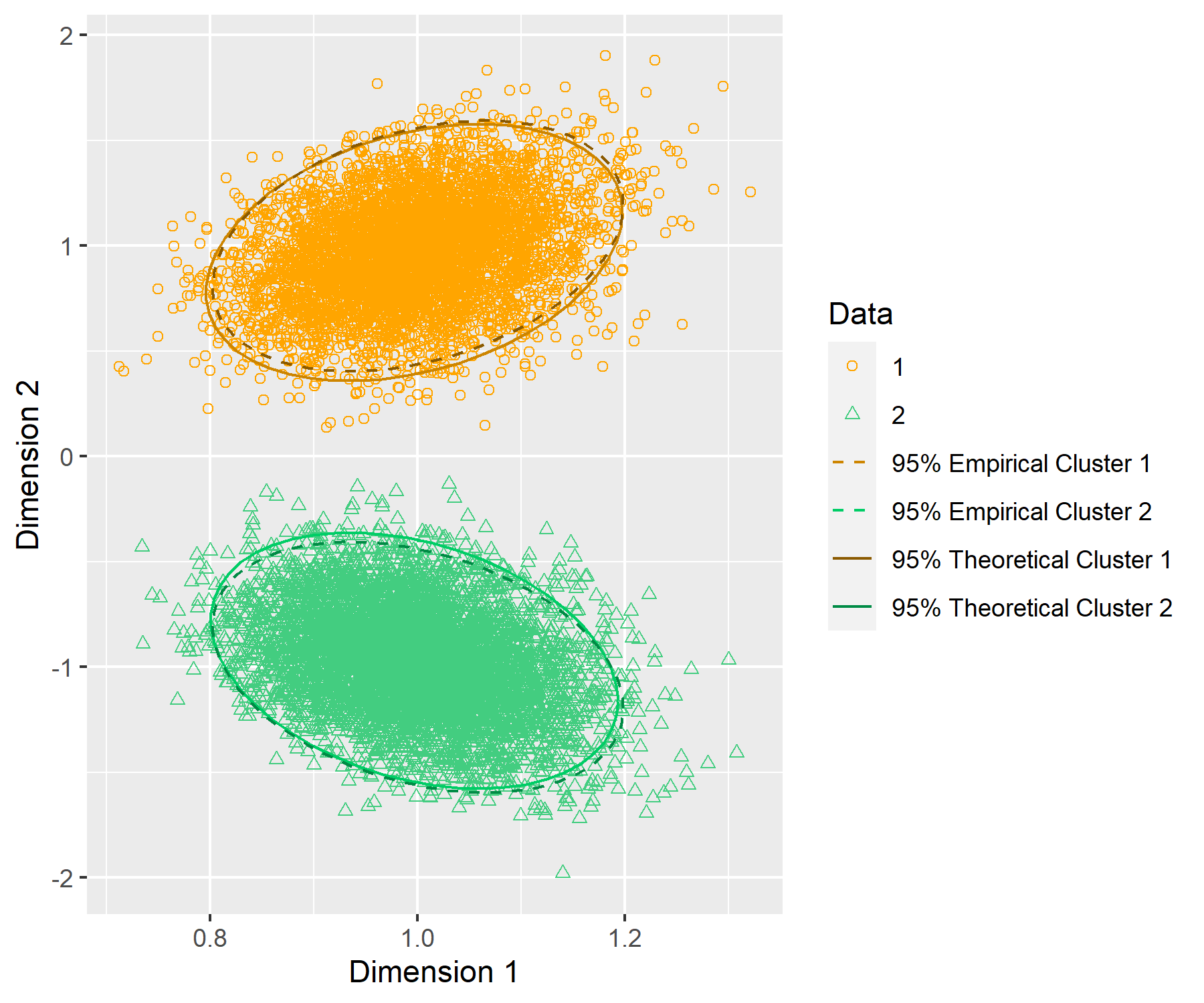
As a preview, consider the specific probability matrix
and consider graphs of size with vertices in each community, also referred to as a specific balanced homogeneous planted partition model. Fig. 1 plots the rows of the matrix whose columns are eigenvectors for the leading two eigenvalues of a single observed adjacency matrix . The dotted lines depict empirical confidence ellipses for each community assuming knowledge of the communities, and the solid lines depict the theoretical confidence ellipses for each community using the per block node-specific asymptotic results in Section 4. The figure illustrates that the rows of the empirical eigenvectors are centered around one of two community-specific centroids. Section 3.1 shows that at the population-level there are in fact distinct, separated community-specific centroids, and Section 3.2 shows that the empirical eigenvectors are, in a well-defined sense, accurately estimating the true eigenvectors. Fig. 1 further alludes to the possibility of approximate asymptotic normality for each vertex embedding which is discussed in greater detail in Section 4.
As illustrated throughout this survey, spectral embeddings can be used for other purposes beyond estimating community memberships, such as parameter estimation (Section 4.7) or hypothesis testing (Section 5).
We remark that certain theoretical properties of spectral embeddings carry over to the model generalizations discussed in Section 2, at times with minor or major modifications. For example, in the degree-corrected stochastic blockmodel, authors have proposed various row-normalization techniques to mitigate the influence of (nuisance) degree parameters when estimating community membership ((Jin, 2015; Jin et al., 2023; Du and Tang, 2021; Fan et al., 2022a). In the mixed-membership stochastic blockmodel, simplices ((Mao et al., 2020) and simplicial ((Jin et al., 2023) geometric structures arise in the latent space which can subsequently be used for statistical inference and modeling. The above references elaborate on the relationships between spectral embeddings and population properties in more general models.
3.1 Population Properties of Spectral Embeddings
To keep discussion succinct and pertinent to later material, this section includes only the adjacency and Laplacian input variants to Algorithm 1 for which asymptotic normality is discussed in Section 4. Here and in the remainder of Section 3 we consider community memberships fixed a priori, with communities and each community having size . In other words, we condition on the community memberships and associated community sizes.
Consider the population adjacency matrix, that is, the matrix whose independent upper-triangular entries satisfy for . Self-edges are permitted for simplicity; the surrounding discussion is not materially different for this section if self-edges are disallowed. Recall that is the matrix whose entries satisfy when vertex belongs to community , and zero otherwise. Write the (skinny) eigendecomposition , where is a matrix whose columns are orthonormal eigenvectors for , and is the diagonal matrix whose entries are the eigenvalues of . Note that if each community has at least one vertex, then the rank of is . Consequently, the eigenvectors of reveal the population-level community memberships in the following sense.
Lemma 1 (Restatement of Lemma 2.1 of Lei and Rinaldo ((2015)).
Suppose is rank , and let be the leading eigenvectors of . There exists a matrix such that . Furthermore, in Euclidean norm, for all .
Given two vertices and such that and , it directly follows that the row differences of satisfy
| (1) |
When is instead rank-degenerate, the row differences can at times be shown to satisfy a similar property.
Lemma 2 (Restatement of Lemma 2 of Zhang et al. ((2022)).
Suppose that , where satisfies
If , then
| (2) |
More general conditions for rank-degenerate matrices are possible such that a lower bound of the form Eq. 2 holds; see Lemma 1 of Zhang et al. ((2022) for further details. If does not change and has constant entries as , then and ; hence in this regime the bound is of order , which matches the lower bound in Lemma 1 for full-rank matrices.
In either the full rank or rank-degenerate case, there are unique rows in corresponding to each of the different communities. Consequently, there are only unique rows of the matrix , whence for some matrix with unique rows corresponding to community memberships.
An alternative approach is to consider the population normalized Laplacian matrix, written as . The normalized Laplacian has a long history in spectral graph theory, with well-known correspondences between eigenvector and eigenvectors with graph connectivity properties ((Chung and Graham, 1997). The normalized Laplacian can also be defined as , but this formulation simply shifts the eigenvalues without affecting the eigenspaces. Writing with eigendecomposition , the following result provides an analogue of Lemma 1 for the normalized Laplacian.
Lemma 3 (Lemma 3.1 of Rohe et al. ((2011)).
If is full rank, then there exists a matrix such that .
The difference between the rows of the matrix is not explicitly given above, but examining the proof, matching notation, and comparing it to Lemma 1 reveals that Eq. 2 holds. Namely, . Hence, for two vertices and such that and , it holds that
| (3) |
In words, knowledge of the eigenvector matrix is again sufficient to recover the community memberships, since there are distinct rows of the eigenvector matrix and the same row corresponds to the same community. As with the population adjacency matrix, directly examining the proof also reveals that , where .
The above observations together show that the spectral embedding of each population similarity matrix reveals community information, in the sense that the population spectral embedding is a fixed transformation of the matrix of community memberships. If the rank of is small relative to , then this spectral embedding can be of much smaller dimension than the similarity matrix. Provided the empirical similarity matrices approximate their population counterparts, in a sense to be quantified in the following subsection, then the corresponding empirical spectral embeddings will approximate their population counterparts as well.
3.2 Subspace Perturbation Approach to Community Detection
There are several concepts of consistent community detection in the large-graph limit: partial recovery, namely recovering vertex memberships better than chance with probability tending to one, weak recovery, namely recovering all but a vanishing fraction of vertex memberships with probability tending to one, and exact recovery, namely recovering all vertex memberships exactly with probability tending to one. Each of these settings has different fundamental information-theoretical limits; see Gao and Ma ((2021) for a survey of minimax rates of estimation and community detection in networks and Abbe ((2018) for a survey of fundamental information-theoretic and computational limits of community detection. In this paper we focus on the regime for which exact asymptotic recovery is possible.
The spectral embeddings of population-level similarity matrices distinguish community memberships, so consistency can be achieved provided that the empirical spectral embeddings are “sufficiently close” to their respective population counterparts. We will first focus on the setting where the spectral embedding is the matrix of leading eigenvectors of the similarity matrix, though the methods used to prove some of the results in this section can also be used to derive results for scaled eigenvectors as well; see Athreya et al. ((2018) and the relevant discussion in Section 4.
In what follows, let denote the eigenvectors computed from an observed, generic similarity matrix, and let denote the eigenvectors of the underlying population similarity matrix. The population and empirical eigenvectors of the adjacency matrix are of dimension , where is the rank of and typically , where but need not be full rank. Consequently, the matrix of eigenvectors grows in size as increases, therefore the convergence of empirical eigenvectors must be defined with respect to an appropriate metric. Since orthogonal projection matrices are unique, metrics on projection matrices offer a natural distance between subspaces; however, note that the cluster information is contained in the rows of the eigenvector matrix . It is therefore natural to consider where denotes a (typically unitarily invariant) norm on matrices such as the spectral or Frobenius norm and are the orthogonal matrices; i.e., the matrices such that . For both the spectral norm and Frobenius norm, classical matrix perturbation theory Bhatia ((1997) provides upper and lower bounds of the form
| (4) |
where and are universal constants depending only on the choice of norm . For example, and ; see Lemma 1 in Cai and Zhang ((2018) or Lemma 2.1.3 in Chen et al. ((2021). These distances are also closely related to the distances between subspaces Bhatia ((1997). In the setting considered herein, these metrics with respect to spectral and Frobenius norms are equivalent up to constant factors, meaning they generate the same metric topology on the set of -dimensional subspaces.
The Frobenius and spectral norm differences between and quantify overall error. Bounding these differences can be shown to yield weak recovery (also described as weak consistency) in certain SBM regimes when using approximate -means clustering, based on the paradigm established in Lei and Rinaldo ((2015). In words, by employing bounds of the above form, Lei and Rinaldo ((2015) proves that a vanishing fraction of vertices get misclustered with high probability for certain large SBM graphs.
To establish strong recovery or perfect clustering, one requires uniform control over the rows of the difference between and . Such uniform control can be established using the norm and the entrywise norm. Here, the norm of a matrix is defined as , i.e., the maximum Euclidean row norm. Consequently, numerous works seek to obtain high-probability bounds for the expression
| (5) |
which is typically achieved indirectly by bounding the proxy
| (6) |
In words, above denotes the solution to the orthogonal Procrustes problem under the Frobenius norm.
In the recent monograph Chen et al. ((2021), the authors develop a generic entrywise bound which is restated here in the particular setting of the stochastic blockmodel.
Theorem 1 (Specialization of Theorem 4.2.1 of Chen et al. ((2021) for SBMs).
Let be rank , and suppose the entries of do not change with . Suppose that for . Suppose that for some sufficiently large constant . Let denote the leading eigenvectors of and let denote the leading eigenvectors of . There exists an orthogonal matrix such that with probability exceeding ,
Obtaining the above result follows from matching notation, observing that the eigenvalues of grow at order , noting that the standard deviation of each entry is bounded by , and the fact that is -incoherent with when (e.g., see Eq. 1). A slightly stronger result can also be stated which yields exact recovery down to the optimal information-theoretic threshold including explicit constants; see Theorem 4.5.1 in Chen et al. ((2021) for details.
The sparsity factor is used to control graph density, balanced against graph size, where often but . If , then it is well-known that the adjacency matrix will no longer concentrate about in spectral norm due to disconnectivity, and if , then with high probability (see e.g., Lei and Rinaldo ((2015) or Remark 3 of Bandeira and Handel ((2016), and see Lu and Peng ((2013) for analogous results about the Laplacian). Furthermore, the information-theoretic limit to achieve perfect clustering is in the regime with explicit constant determined in some important special cases; see Abbe ((2018).
A host of authors have studied eigenvector perturbations in statistical models, often in the context of network analysis ((Agterberg et al., 2022; Abbe et al., 2020, 2022; Cai et al., 2021; Cape et al., 2019a, c; Eldridge et al., 2018; Jin et al., 2023; Lei, 2019; Lei et al., 2020b; Rohe and Zeng, 2020; Yan et al., 2021; Zhang and Tang, 2022b). For the setting of stochastic blockmodels with fixed matrix, these results all translate to similar statistical consequences: if and , then the row-wise error between and , after proper orthogonal alignment, is sufficiently small. Since the rows of reveal the community memberships per Eq. 1, these results suggest that exact community recovery occurs with probability tending rapidly to one for sufficiently dense graphs, namely with sparsity parameter satisfying . Moreover, consistent estimation of the -th row of uniformly over all rows paves the way for further downstream inference and cluster analysis.
4 Asymptotic Normality in Stochastic Blockmodels
Asymptotic normality, manifest through the centering (asymptotic mean) and scaling (asymptotic variance) provides a more refined characterization of cluster geometry and spectral embeddings beyond consistency. Further, distributional theory is conventionally a precursor to developing statistical inference procedures, so the asymptotic normality results developed in this section enable inference procedures based upon spectral embeddings. Section 4.1 discusses limiting results for the unscaled eigenvectors, and Section 4.2 presents limiting results for other embeddings, followed by a discussion of the relationship between these various results in Section 4.4. Section 4.6 discusses the asymptotic normality of the empirical eigenvalues and concludes by examining how these results enable parameter estimation.
4.1 Asymptotic Normality of the Adjacency Matrix Eigenvectors
Perhaps the conceptually simplest spectral embedding is the leading eigenvectors of the adjacency matrix . A first result quantifying the fluctuations of the rows of about their corresponding means is in Theorem 2 of Cape et al. ((2019a), which focuses on the special case that the block probability matrix is positive semidefinite.
Theorem 2 (Restatement of Theorem 2 of Cape et al. ((2019a) for SBMs).
Suppose that , that , and that and remain constant as . Write for some matrix . There exists a sequence of orthogonal matrices and depending on such that
where the asymptotic covariance matrix is given by
where the matrices and are given by
provided these limits exist.
When the communities are instead randomly generated according to , the limiting matrices and exist almost surely by the law of large numbers. In this case, a key property of the limiting matrix is that it depends only on the membership , the community probabilities and the particular block probability matrix . Since, per Section 3.1, there are at most unique values of , with each distinct row corresponding to a covariance matrix , this result suggests that asymptotically behaves like a mixture of Gaussian random variables, where the mixture components are associated to the different community centers.
If the community sizes are of comparable sizes, such as when the relative community membership proportions are held fixed, then by Eqs. 1 and 2, the row norms of the population eigenvectors are necessarily tending to zero simultaneously and at the same rate; this property reflects incoherence ((Chen et al., 2021). From a statistical standpoint, this “shrinking to zero” property is reflected in the scaling required to obtain a Gaussian limit. Informally, the scaling decomposes as the product where the term accounts for the incoherence and the term is the square root of the “effective sample size;” that is, it is the sample size after accounting for the additional edge sparsity. In the absence of the sparsity, namely in the fully dense regime, the classical parametric rate is obtained after adjusting for the eigenvector incoherence. Furthermore, notice that the rate appears in the denominator of the bound in Theorem 1.
The full result stated in Cape et al. ((2019a) is more general and permits for an matrix ; see Section 4.2 for an interpretation of this assumption. Notice that there are two distinct orthogonal matrices appearing in the asymptotic normality result for ; the matrix stems from the alignment of to , whereas the the additional matrix globally rotates the difference . This presence of the second orthogonal matrix enables specifying the limiting covariance matrix . Subsequently, Xie ((2022) extends the central limit theorem for the eigenvectors in Cape et al. ((2019a) to sparsity of order and deterministic sequences of positive semidefinite matrices under technical conditions on .
Theorem 3 (Restatement of Theorem 4.4 of Xie ((2022) for SBMs).
Suppose that , that and remain constant as , and suppose that for some (constant) matrix . Suppose further that there exists a constant such that . Define
with
Suppose that is fixed in and that for . Let denote a Gaussian random variable in with identity covariance matrix. There exist sequences of orthogonal matrices and depending on such that for any convex measurable set it holds that
The result is actually more general, permitting positive semidefinite matrices, to grow with , and to change in . Explicitly, Theorem 3 demonstrates that the rows of the empirical eigenvectors are asymptotically Gaussian about the rows of with covariance determined by , where the matrix can be viewed as the finite-sample approximation of the matrix in Theorem 2. A key difference between Theorem 2 and Theorem 3 is that in Theorem 3, need not be converging as , whereas Theorem 2 assumes that converges as . Furthermore, Theorem 3 is nonasymptotic in . The rate of convergence of the cumulative distribution functions also clarifies the role of as the effective sample size: for classical finite-dimensional Berry-Esseen Theorems, the rate of convergence to the Gaussian cumulative distribution function is of order ; in Theorem 3, it is of order modulo logarithmic terms.
Observe that , namely, view the -th entry of the -th row of as the inner product of the -th eigenvector with the standard basis vector . In Fan et al. ((2020) the authors develop asymptotic theory for general linear forms where is a user-specified deterministic unit vector. In particular, their Theorem 2 establishes that
| (7) |
where , and are defined according to population parameters, as well as the parameters , , and . Explicitly, is shown to solve the fixed-point equation
| (8) |
over an interval that contains but no other eigenvalues, thereby implicitly precluding the possibility of repeated eigenvalues. Here is defined as
where is some sufficiently large integer defined in their proof, and where and denote the matrices and with the entries associated to the -th eigenvector and eigenvalue removed. See Section 4.6 for further discussion of the quantity . Lemma 3 of Fan et al. ((2020) shows that is well-defined and satisfies as . The definitions of , and appearing in Eq. 7 are quite involved, yet in special cases they admit simple asymptotic expressions, such as by taking , which corresponds to the cosines of the angles between the empirical and true eigenvectors.
Theorem 4 (Restatement of Part 2 of Theorem 2 in Fan et al. ((2020) for SBMs).
Suppose that for some constant , and suppose that , where and remain constant as . Suppose also that has distinct eigenvalues satisfying for some constant for . Suppose that is fixed in with , and let be the solution to the fixed-point equation in Eq. 8. Suppose that . Then,
where the centering term has the expansion
The above presentation differs from the original statement in Fan et al. ((2020) but follows by observing that the eigenvalues of are of order when is fixed, the parameter appearing in Fan et al. ((2020) is of order , and the fact that the eigenvectors are incoherent when . In essence, Theorem 4 demonstrates that the cosines of the angles between empirical and population eigenvectors are asymptotically Gaussian with mean one minus a bias term stemming from second-order moment properties via and variance determined by fourth-order moment properties via . The results in Fan et al. ((2020) cover other situations, including demonstrating different asymptotic phenomena based on whether the deterministic vector is incoherent, as well as results for dense and sparse networks.
By Eq. 4, the eigenvector difference is closely related to the projection norm difference, and hence by analogy the distributional asymptotics for the matrix are closely related to the difference . The theory in Fan et al. ((2020) reflects this relationship; more specifically, their limit results for the linear form are based on first developing asymptotic expansions for the term for sequences of deterministic unit vectors and , which is the the bilinear form generated by the difference of projections onto the -th dominant eigenspace. This investigation differs from the row-wise joint focus on the collection of leading eigenvectors in Theorems 2 and 3.
The asymptotic theory presented in Fan et al. ((2020) allows to have negative eigenvalues but requires that the eigenvalues of be distinct, which is needed to explicitly quantify the fluctuations of the individual eigenvectors . Both Theorem 2 and Theorem 3 require that is positive semidefinite, but they allow for repeated eigenvalues of the matrix ; as a consequence, Theorems 2 and 3 can only quantify the fluctuations of the rows (as opposed to entries) of the matrix of leading eigenvectors up to orthogonal transformation (as opposed to individual eigenvectors ). Furthermore, the results in Fan et al. ((2020) require a sparsity parameter that satisfies for some , which does not allow to grow as polylog. In contrast, Theorems 2 and 3 allow much sparser networks.
Instead of considering the rows or entries of or , Li and Li ((2018) consider a modified Frobenius distance between and , up to orthogonal transformation. When the stochastic blockmodel in question is a balanced homogeneous stochastic blockmodel, the limiting mean and variance of their modified Frobenius norm error admits a simple analytical expression closely related to the distance.
Theorem 5 (Restatement of Theorem 3 of Li and Li ((2018)).
Suppose that is of the form
where are constants. Suppose and that each community has precisely vertices, where remains constant as . Suppose further that for some . There exists a sequence of orthogonal matrices such that
where and are defined via
In fact, Li and Li ((2018) allows and to change with but this is omitted above for ease of presentation. The proof in Li and Li ((2018), after establishing the initial expansion, uses a path-counting technique from random matrix theory to prove asymptotic normality, where the simple parameterization allows for convenient analysis of each term which leads to the appealing closed-form expressions for the mean and the variance . Whether this result can be generalized to the setting of general matrices and sparsity of order , or even for , remains an open problem.
The random variable can informally be viewed as a re-weighted Frobenius distance with respect to the magnitude of the eigenvalues. Recall that Theorem 4 demonstrates that the cosines of the eigenvectors between and have an asymptotically normal distribution after appropriate scaling and centering. The results of Fan et al. ((2020) do not imply the limiting results of Li and Li ((2018), as the former requires distinct eigenvalues and the latter operates under a specific model with repeated eigenvalues (in fact, the model in Li and Li ((2018) has repeated eigenvalues). However, both theorems reflect similar asymptotic normality properties for the (rescaled) sines or cosines between the empirical and true eigenvectors, suggesting that it may be possible to extend these results to the setting as in Cape et al. ((2019a), though additional techniques as in Xie ((2022) may be required for .
Finally, both Fan et al. ((2020) and Li and Li ((2018) include distributional theory pertaining to the sines and cosines between empirical and population eigenvectors. In contrast, Cape et al. ((2019a) and Xie ((2022) considers distributional theory for individual rows. The scaling to obtain asymptotic normality for the rows may not be the same as the scalings for the asymptotic normality for the sines and cosines of the eigenvectors; informally, this is because both sines and cosines of the eigenvectors are global fluctuations (i.e., aggregated over the entries), whereas Cape et al. ((2019a) and Xie ((2022) consider the pointwise, local fluctuations.
4.2 Asymptotic Normality for Scaled and Laplacian Eigenvectors
An alternative graph embedding approach is to scale the leading eigenvectors by the square roots of the corresponding eigenvalue magnitudes. This scaling has a convenient interpretation through the so-called latent space model, which assumes that each vertex has a Euclidean representation lying in some low-dimensional latent space. The general latent space model posits that the entries of the matrix are obtained by first drawing points as latent Euclidean vectors from some distribution on , and then the entries of are set via , where is a symmetric kernel function that maps two Euclidean points to the unit interval. In the particular case that , one obtains the random dot product graph.
Definition 4 (Random dot product graph – undirected, loopy).
We say an adjacency matrix is a random dot product graph on vertices with sparsity factor if, conditional on satisfying , the upper-triangular entries of the adjacency matrix are generated independently in the manner
The rows of the matrix may be deterministic or modeled in a generative fashion via i.i.d. for some distribution on .
The random dot product graph has the property that , where each row of is interpreted as a latent position in . In this setting, for some orthogonal matrix (not necessarily identifiable). Consequently, the scaled eigenvectors correspond to an isometric linear transformation and scaling of the original latent vectors. The latent-space interpretation avoids the previous shrinking-to-zero phenomenon from the eigenvectors in , though not necessarily in the sparsity factor , and introduces additional regularity into the definition of whose entries are pairwise evaluations of inner products, while still maintaining graph heterogeneity via the distribution of the latent vectors.
A survey of statistical inference under the random dot product graph can be found in Athreya et al. ((2018). Our focus herein is on asymptotic normality for random dot product graphs through the lens of stochastic blockmodels.
4.2.1 Latent Space Interpretation of the Stochastic Blockmodel
Interpreting the stochastic blockmodel as a latent space model amounts to imposing an additional assumption on the distribution if the communities are stochastic or on the rows of the matrix if the communities are deterministic. Namely, either corresponds to a mixture of point masses in , where is the rank of , or has at most unique rows, with each row corresponding to community membership in the latter if the communities are fixed. One manner to specify the distribution is via the eigendecomposition of the matrix ; if is positive semidefinite, let be its eigendecomposition, and let denote the matrix . Then, the rows of can be drawn via whence , so the stochastic blockmodel is a random dot product graph. In fact, Theorems 2 and 3 hold under the more general condition for some matrix , modulo additional technicalities, where the factorization gives rise to the asymptotic covariance matrices and . We note that the latent space interpretation also extends to the various stochastic blockmodel extensions mentioned in Section 3.2. For the mixed-membership stochastic blockmodel, the latent space interpretation implies that the latent positions belong to a simplex in dimensions, and for the degree-corrected stochastic blockmodel the latent positions are one of rays emanating from the origin, where each ray corresponds to a different community ((Du and Tang, 2021).
Let have leading eigenvectors as before, and let the corresponding diagonal matrix of eigenvalues be denoted as . In particular, write , where consists of the eigenvectors and eigenvalues corresponding to the largest in magnitude eigenvalues of . Write . It can be shown that , where is an orthogonal transformation. Recall that since , then for some orthogonal matrix , which in particular suggests that , where is a possibly different orthogonal transformation representing the product of different, underlying orthogonal transformations.
In fact, the matrix of scaled eigenvectors exhibits similar uniform row-wise convergence guarantees as the unscaled eigenvectors ((Rubin-Delanchy et al., 2022; Athreya et al., 2018).
Theorem 6 (Modification of Theorem 5 of Rubin-Delanchy et al. ((2022)).
Suppose and remain constant as , and let , where each is drawn according to independently with the ’th row of , and let denote the rank of . There exists a universal constant and an orthogonal matrix such that provided ,
with probability at least for any prespecified choice of constant . The value of influences the implicit constant in the big-O bound.
See also Athreya et al. ((2018). This entrywise perturbation result has been extended in Xie ((2022) to the setting that . For sufficiently dense graphs, the convergence of to resembles the convergence of to after accounting for the order of magnitudes: for sufficiently dense graphs, , there exist sequences of orthogonal transformations and depending on such that with high probability,
establishing that the relative row-wise error for both and tends to zero as the number of vertices tends to infinity.
4.2.2 Asymptotic Normality for the Scaled Eigenvectors
In Athreya et al. ((2016), the authors prove a central limit theorem for the scaled eigenvectors of random dot product graphs under the assumption that the latent positions are sampled from a distribution on provided that the second moment matrix has distinct eigenvalues. This result is extended in Athreya et al. ((2018) to the setting where the second moment matrix is permitted to have repeated eigenvalues. For positive semidefinite stochastic blockmodels with equal probabilities of community membership, the assumption of distinct eigenvalues of is equivalent to the assumption that have distinct eigenvalues, but for unequal community membership probabilities the eigenvalues of need not be the same as those of . In fact, it is straightforward to check that , where the matrix is the matrix of distinct latent vectors associated to the corresponding stochastic blockmodel.
Theorem 7 (Restatement of Corollary 1 of Athreya et al. ((2018)).
Suppose that does not change and has constant entries as . Suppose that . Let , and suppose . There exists a sequence of orthogonal matrices depending on such that
where the asymptotic covariance matrix is given by
where
Just as in the asymptotic results for the unscaled eigenvectors, Theorems 2 and 3, the covariance matrix depends on the community probabilities , the membership of the -th vertex, and the block probability matrix . Theorems 2 and 3 share the asymptotic covariance
Consequently, Theorem 7 demonstrates that the asymptotic covariance matrices for the scaled and unscaled eigenvectors are related via
which reflects the additional scaling of the eigenvectors by the eigenvalues. Theorem 7 requires that the average expected degree grows linearly in , which can be unrealistically restrictive. Tang and Priebe ((2018) generalizes this result to the setting .
Theorem 8 (Restatement of Theorem 2.2 of Tang and Priebe ((2018)).
Suppose that and remain constant as , and suppose that . Suppose further that and that . There exists as a sequence of orthogonal matrices depending on such that
| (9) |
where the asymptotic covariance matrix satisfies
with as in Theorem 7 and defined as
More recently, Xie ((2022) extends this result to the regime , which builds upon work in Xie and Xu ((2021) for sequences of deterministic matrices , rather than stochastically generated community memberships.
Theorem 9 (Restatement of Theorem 4.4 of Xie ((2022) for SBMs).
Similar to Theorem 3, Xie ((2022) obtains a finite-sample result and hence allows to change with or the communities to be small.
Taken together, Theorems 7, 8 and 9 demonstrate a similar phenomenon as occurs for the unscaled eigenvectors: the estimated scaled eigenvectors are approximately Gaussian around block-specific centroids after appropriate orthogonal transformation. An important difference between scaled and unscaled eigenvectors is that for scaled eigenvectors the cluster centroids do not depend on besides through the sparsity factor , which, for practical purposes, can be estimated consistently after imposing an identifiability condition (e.g., or ).
When the kernel associated to a general latent position random graph is of the form , the corresponding block probability matrix will necessarily be positive semidefinite. In Rubin-Delanchy et al. ((2022), the authors introduce the generalized random dot product graph model, which replaces the inner product with a pseudo-inner product to model large in-magnitude negative eigenvalues of the adjacency matrix and hence allow for indefinite matrices.
Definition 5 (Generalized random dot product graph – undirected, loopy).
An adjacency matrix for a generalized random dot product graph on vertices with sparsity factor has independent upper-triangular entries where
where satisfies and is the matrix with . The rows of the matrix may be deterministic or modeled in a generative fashion via i.i.d. for a distribution on .
Here, as for RDPGs, the construction of the corresponding latent position distribution is again a mixture of point masses, if , defined by , with and representing the number of positive and negative eigenvalues of respectively. Under the generalized random dot product graph model, the matrix can be decomposed as , but the definition induces an additional nonidentifiability. If is a matrix satisfying , then and generate the same probability matrix, implying that the latent positions are only identifiable up to transformations satisfying this identity; these matrices are called the indefinite orthogonal matrices. Consequently, analyzing the generalized dot product graph requires additional considerations with respect to these transformations . For random dot product graphs, namely when , these matrices are simply orthogonal matrices.
Rubin-Delanchy et al. ((2022) extends Theorem 8 to the generalized random dot product graph setting.
Theorem 10 (Restatement of Theorem 2 of Rubin-Delanchy et al. ((2022) for SBMs).
Suppose and remain constant as with , and let , where and correspond to the largest in magnitude positive and negative eigenvalues of . There exist sequences of orthogonal matrices and indefinite orthogonal matrices and a universal constant such that, provided the sparsity factor satisfies , then
where the asymptotic covariance matrices satisfy
The asymptotic covariances for both and are direct extensions of those in the positive semidefinite case Theorems 7 and 8 but now reflect the roles of the leading eigenvalue signs through the matrix . Furthermore, an additional indefinite orthogonal matrix appears on the left hand side of Theorem 10. A key property of indefinite orthogonal matrices is that they preserve volumes, since , so that the asymptotic Gaussianity is retained in the sense that the volume of the ellipsis generated by these asymptotic covariance matrices is invariant to these transformations. More discussion about these matrices and their properties as they pertain to inference for general latent position random graphs can be found in Rubin-Delanchy et al. ((2022). Note that this result reduces to the special case of asymptotic normality in the positive semidefinite matrix setting by taking . These results may extend to the regime using the techniques in Xie ((2022).
Theorem 10 demonstrates that the rows of the matrix are approximate Gaussian about the rows of . As before, there are only unique centroids, where the centroids correspond to community memberships. Results presented earlier only involve orthogonal transformations, whence the cluster shape, in the sense of the ellipsis generated by the covariance, is determined by the asymptotic covariance matrix in the statement of the result, whereas in Theorem 10 the cluster shape is determined by both the limiting asymptotic covariance as well as the nonidentifiable indefinite orthogonal matrix .
4.2.3 Asymptotic Normality for the Laplacian Eigenvectors
Thus far, the results discussed emphasize embeddings obtained from the adjacency matrix . In Tang and Priebe ((2018), the authors prove central limit theorems for the scaled eigenvectors of the Laplacian under the random dot product graph model, which is stated in the following theorem.
Theorem 11 (Corollary 3.3 of Tang and Priebe ((2018)).
Suppose that and remain constant as with . Let be the leading eigenvectors of scaled by the square roots of the corresponding eigenvalues. Define the matrices
Suppose that . There exists a sequence of orthogonal matrices such that
where the asymptotic covariances are defined via
This result was later extended to the generalized random dot product graph in Rubin-Delanchy et al. ((2022) and to sequences of deterministic matrices in Xie and Xu ((2021).
The terms that appear in the denominators of the quantities in Theorem 8, such as , can be interpreted as the average degree within community , and the centering term can be understood as the latent vector associated with community , normalized by the square root of the expected degree within that community. Such a term arises when considering the normalized Laplacian, which normalizes to account for nodal degree heterogeneity. The scaling to obtain asymptotic normality in Theorem 8 is , which demonstrates a similar “shrinking to zero” phenomenon as the unscaled eigenvectors of the empirical adjacency matrices.
In Theorem 11, the matrices and are more involved than the corresponding covariance matrices in Theorem 2 or Theorem 7, though they are completely determined by community membership probabilities , the matrix , and the membership of the -th vertex. Since the matrices and are different, in Tang and Priebe ((2018) the authors consider model settings for which using the scaled eigenvectors of the Laplacian matrix is preferred to using the adjacency matrix for spectral clustering, on the basis of Chernoff information. This idea was further explored in Cape et al. ((2019b).
In Modell and Rubin-Delanchy ((2021), the authors consider the scaled eigenvectors of the random walk Laplacian defined as the matrix
where is the diagonal matrix of degrees. Note that has real eigenvalues since it is related by matrix similarity to the matrix , whence is well-defined.
Theorem 12 (Restatement of Theorem 4.2 of Modell and Rubin-Delanchy ((2021)).
Define as in Theorem 11, and suppose that and remain constant as . Denote
There exists an sequence of indefinite orthogonal matrices and a constant such that provided , then
where the asymptotic covariance matrices are given by
Modell and Rubin-Delanchy ((2021) studies the performance of the random walk embedding for clustering under the degree-corrected stochastic blockmodel. The proofs therein use the tools developed in Tang and Priebe ((2018) and Rubin-Delanchy et al. ((2022), together with the fact that if is an eigenvector of , then is an eigenvector of . The limiting covariance is similar to the result in Theorem 11 because of the close relationship between the eigenvectors of and those of . The authors also consider how this embedding behaves under the degree-corrected stochastic blockmodel, in particular avoiding a form of distortion induced by other degree-normalization procedures, but this is beyond the scope of the present survey.
4.3 Abridged Glossary of Asymptotic Normality Results for Scaled and Unscaled Eigenvectors
For convenience and reference we provide Table 1 summarizing the works discussed thus far.
| Paper | Asymptotic normality | Sparsity | Model |
|---|---|---|---|
| Athreya et al. ((2016) | Rows of scaled eigenvectors of adjacency matrix | , i.i.d. rows of drawn, distinct eigenvalues | |
| Cape et al. ((2019a) | Rows of unscaled eigenvectors of adjacency matrix | ||
| Fan et al. ((2020) | Linear forms of distinct unscaled eigenvectors of adjacency matrix | , | low-rank and distinct eigenvalues |
| Li and Li ((2018) | Squared Frobenius norm difference of scaled eigenvectors | , with a balanced homogeneous stochastic blockmodel | |
| Modell and Rubin-Delanchy ((2021) | Rows of , where are the eigenvectors of the Laplacian and are the degrees | , i.i.d. rows of | |
| Rubin-Delanchy et al. ((2022) | Rows of scaled eigenvectors of adjacency and Laplacian matrix | , i.i.d. rows of | |
| Tang and Priebe ((2018) | Rows of unscaled eigenvectors of Laplacian matrix | , i.i.d. rows of drawn | |
| Xie and Xu ((2021) | Rows of scaled eigenvectors of adjacency matrix | ||
| (above) | Rows of one-step updated scaled eigenvectors (see Section 4.7.1) | ||
| (above) | Rows of scaled eigenvectors of Laplacian matrix | Either and or with an SBM | |
| (above) | Rows of one-step updated scaled eigenvectors (see Section 4.7.1) of Laplacian matrix | ||
| Xie ((2022) | Rows of scaled and unscaled eigenvectors of adjacency matrix | ||
| (above) | Rows of one-step updated scaled eigenvectors (see Section 4.7.1) |
4.4 Relationships Between Limiting Results for Eigenvectors
Similar to the entrywise perturbation results discussed in Section 3.2, the results in Sections 4.1 and 4.2 illustrate a common theme: for sufficiently dense graphs, each row of the embedding in question after multiplication by a standardization factor is asymptotically Gaussian about one of different centroids in , where the location of the centroid depends on the particular embedding specification. Furthermore, aggregating rows also results in asymptotic normality, per Theorems 4 and 5.
Underlying many proofs in the aforecited works are the characterizations
| (10) | ||||
where and are residual matrices whose norm is comparatively small with high probability for large graphs. Similar characterizations hold for other spectral embeddings for networks (e.g., Theorem 3.1 in Tang and Priebe ((2018)) or spectral methods more generally (e.g., Lemma 4.18 in Chen et al. ((2021)). The primary technical difficulty is that isolating leading-order terms requires some care. There are multiple different approaches and avenues to obtain such expansions; for example, Fan et al. ((2020) uses techniques from random matrix theory, Cape et al. ((2019a) uses techniques from matrix perturbation theory, and Xie ((2022) uses a “leave-one-out” technique also used in Abbe et al. ((2020) for developing perturbation bounds for eigenvectors; see also Chen et al. ((2021).
The appearance of the orthogonal matrix stems from the fact that the eigenvalues need not be distinct. However, Lemma 9 in Fan et al. ((2022a) shows that when the eigenvalues are distinct, a similar entrywise expansion holds for the individual eigenvectors.
Lemma 4 (Restatement of Lemma 9 of Fan et al. ((2022a) for SBMs).
Suppose that for some constant , and suppose that . Suppose also that has distinct eigenvalues satisfying for . Suppose that and remain constant as with . Then it holds that
where is the solution to the fixed-point equation in Eq. 8.
This result is in fact a special case of Theorem 3 of Fan et al. ((2020). The asymptotic expansions in Eq. 10 can be understood to hold for equal to a sign matrix when the eigenvalues are sufficiently separated. Explicitly, this leading-order expansion demonstrates that the entries of the -th eigenvector have a variance that is asymptotically proportional to the -th eigenvalue, a phenomenon that has also been shown in non-network settings (e.g., Agterberg et al. ((2022)). Lemma 4 demonstrates that when the eigenvalues are distinct the asymptotic variance is proportional to the quantity ; however, the difference between and can be shown to be asymptotically negligible for sufficiently dense networks. For further details regarding , see Section 4.6.
In Li and Li ((2018), the authors prove the distributional convergence of the random variable to a Gaussian random variable. This term can be viewed as a modification of the (Frobenius) distance between the eigenvectors, cf. Section 4.1. We are unaware of analogous results in the literature for the distance itself, but there are several concentration inequalities for the random variable – see Tang and Priebe ((2018); Tang et al. ((2017a); Agterberg et al. ((2020) for statements of these results in the settings of random dot product graphs and generalized random dot product graphs. The proof of these results is markedly similar to the proofs of the asymptotic normality guarantees; after establishing the asymptotic expansion one must analyze the fluctuations of the leading term about its expectation. For the random variable considered in Li and Li ((2018), the leading term is simply which is amenable to analytical calculations for model studied therein.
Asymptotic multivariate normality results by themselves do not address consistent estimation of the limiting covariance matrix for each row, which would be necessary to devise asymptotically valid confidence regions or provide data-driven uncertainty quantification. In Section 5, we review hypothesis testing settings where consistent estimation of the limiting covariance is possible.
4.5 Cluster Structure: A Simple Numerical Example
The asymptotic normality results for the -th row presented in the previous subsections have limiting covariance matrices that depend on the matrix and the community membership of the -th vertex. The resulting cluster geometry is impacted by the particular form of these covariance matrices. Consider, for example, the setting where , , , with equal size communities. Note that the leading eigenvector of is simply the constant vector. In addition, the second eigenvector is the vector whose entries are with sign corresponding to community membership. Consequently, since unit-norm eigenvectors are only defined up to sign, by symmetry one must have that for or , and that , where denotes the asymptotic covariance obtained from Theorem 2. Consequently, the covariance matrices are of the form
written in terms of underlying, implicit parameters , , and . Fig. 1 showcases this phenomenon, where the covariance for class one appears positive for dimensions one and two, whereas the covariance between dimensions one and two for class two appears negative. However, this observation does not necessarily result in nearly spherical covariance matrices.
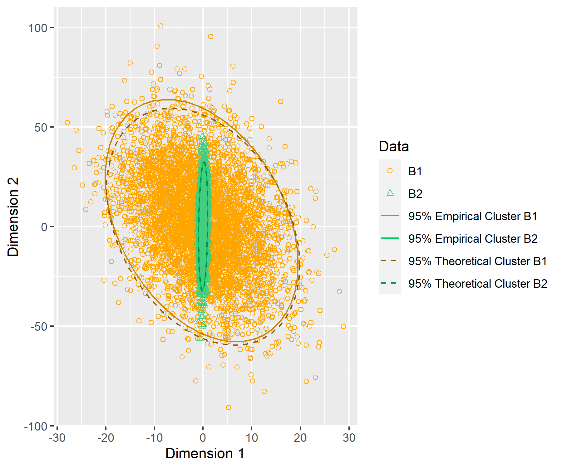
Consider two possible connectivity matrices
with exactly vertices in each community. The leading eigenvectors of and are the same, but the resulting covariance matrices are different as they depend on the entries of . In Fig. 2, we plot the first rows of for and respectively. Here, has a condition number of , whereas has a condition number of , resulting in covariance condition numbers of and respectively. The cluster associated to is visibly much more elongated – though the network is denser than the corresponding network drawn from the matrix , the resulting covariance matrix is highly elliptical. Computing the theoretical limiting covariance numerically yields
which showcases the effect of ill-conditioned matrices on cluster structure. While the asymptotic normality results presented hold for fixed matrices as , the limiting covariance structure depends highly on the matrix , and even sufficiently dense networks may still exhibit manifestly different cluster structure in latent space.
4.6 Empirical Eigenvalues
Eigenvalues of random matrices are well-studied in the field of random matrix theory. Per the aim of this survey, we focus on asymptotic normality guarantees, and only discuss limiting results concerning the top in magnitude eigenvalues of .
Among the numerous existing works that establish asymptotic normality for eigenvalues, the following classical result establishes the limiting behavior of the leading eigenvalue of an Erdős–Rényi random graph.
Theorem 13 (Restatement of Theorem 1 of Füredi and Komlós ((1981)).
Suppose with where is fixed. Then, as ,
Since the leading eigenvalue of the edge probability matrix of an Erdős–Rényi random graph is simply when permitting self-edges, this result shows that the leading empirical eigenvalue is asymptotically normal about the leading population eigenvalue modulo a small, constant-order bias term.
More recently, Theorem 13 has been extended to the more general rank setting for stochastic blockmodels as follows.
Theorem 14 (Restatement of Theorem 3 of Athreya et al. ((2021) for SBMs).
Suppose that and that . Let and remain constant as . Let denote the unit norm eigenvector satisfying
where is the -th nonzero eigenvalue of . Define the vector . Let denote the -dimensional vector with components
and let denote the matrix with elements
Then,
The vector is also shown to converge when the eigenvalues of are assumed distinct (see their Theorem 2). Furthermore, similar to Theorem 13, it can be shown that and are bounded bias and variance terms. Explicitly, is the limiting value of the variance of the random variable after unconditioning on the latent vectors . Here is order as the authors assume that . The results are derived under the general latent-space framework of the generalized random dot product graph described in Section 4.2.
A closely related marginal result for individual eigenvalues is stated in the following theorem.
Theorem 15 (Restatement of Theorem 1 of Fan et al. ((2020) for SBMs).
Let with and constant as , and suppose that for some . Suppose also that has distinct eigenvalues satisfying for some constant for . Suppose that is fixed in with . Then,
where is the unique solution to the fixed-point equation defined in Eq. 8.
Theorems 14 and 15 are not easy to directly compare. In Fan et al. ((2020), the authors do not consider a latent-space framework, so the eigenvalues of need not converge. Since , and the nonzero eigenvalues of a generic matrix product are the same as the nonzero eigenvalues of the matrix product , the nonzero eigenvalues of are the same as those of . If each row of is drawn from a latent position distribution, then almost surely, so the eigenvalues of are converging to the eigenvalues of . As a consequence, their results allow for more sparsity a priori by only specifying a sequence of matrices . In fact, they require that for some , which is not as sparse as the information-theoretic threshold required for consistency in community detection but is significantly sparser than the fully dense regime studied in Athreya et al. ((2021).
In principle, the eigenvalue result in Theorem 15 should match Theorem 14 under the conditions specified in the latter, though explicitly verifying this is technically involved. While the bias (centering) term in Athreya et al. ((2021) is computed directly, the bias term in Fan et al. ((2020) is expressed implicitly through the solution of a complex analytic fixed-point equation. On the other hand, the limiting variances are seen to be comparable since both stem from , so one need only check that the biases match.
Both Theorem 15 and Theorem 14 consider the fluctuations of the eigenvalues at the scaling . Under the latent space framework, the eigenvalues of can be viewed as an empirical kernel matrix with kernel . The results of Koltchinskii and Gine ((2000) imply that the eigenvalues of are approximately Gaussian about the eigenvalues of a corresponding integral operator, which in this case are simply the eigenvalues of . Therefore, the fluctuations of the eigenvalues of may be approximated by the eigenvalues of the normalized matrix or . These eigenvalues are studied in the context of a general low-rank random graph in Lunde and Sarkar ((2019).
Theorem 16 (Restatement of Theorem 3.1 of Lunde and Sarkar ((2019) for SBMs).
Suppose that and remain constant as , that , and that . Suppose that the eigenvalues of are distinct. Then,
where denotes the asymptotic covariance matrix.
Lunde and Sarkar ((2019) allows the probabilities to be drawn from a general latent position distribution but requires that . The authors do not provide the covariance matrix , but it should be noted that it is the same as in Koltchinskii and Gine ((2000); in essence, this is due to the fact that the fluctuations of are of smaller order than the fluctuations of and its corresponding integral operator. In other words, the leading eigenvalues of and have the same limiting distribution. In contrast, the results in Athreya et al. ((2021) and Fan et al. ((2020) concern the leading eigenvalues of .
Taken together, these results imply that for sufficiently dense graphs the empirical eigenvalues of are biased estimators of the eigenvalues of , but, the eigenvalues of are unbiased estimators of those of the corresponding kernel operator. Whether these results can be extended to various sparsity regimes or can be used explicitly for inference is an open question.
4.7 Parameter Estimation
When the community memberships are viewed as stochastic and when and are assumed known, the model parameters are encapsulated in . Absent additional structural assumptions, consists of unconstrained parameters in , while consists of nonnegative parameters in that sum to unity. Community memberships are unique only up to a global permutation of community labels (i.e., global relabeling), so strictly speaking, estimation of the matrix holds up to simultaneous row/column permutation, while estimation of the vector holds up to a permutation of its coordinates.
The likelihood function of and of when permitting self-edges are each given by
| (11) | ||||
| (12) |
For stochastic blockmodel graphs governed by parameters where and are assumed known, the maximum likelihood estimate of and is given by
| (13) |
The asymptotic normality of the maximum likelihood estimate was obtained in Lemma 1 of Bickel et al. ((2013) in the asymptotic regime , with implicit limiting variances (see Tang et al. ((2022) for additional discussion).
Theorem 17 (Reformulation of Lemma 1 of Bickel et al. ((2013)).
Suppose and remain constant as , and suppose with with . Let denote the MLE of obtained from with assumed known. If , then
| (14) |
If with , then
| (15) |
In either case, the random variables are asymptotically independent.
The likelihood in Eq. 12 can be computationally expensive, and is in general NP-hard to compute ((Amini et al., 2013). Furthermore, as discussed in Section 4, when specifying a stochastic blockmodel matrix having dimension , there is no a priori reason to assume that has full matrix rank equal to . This observation is important for determining the true number of model parameters for estimation, i.e., loosely speaking, an upper bound on the complexity of the SBM parameter estimation problem. As , then by taking the spectral decomposition of , there are at most total parameters, via the eigendecomposition of .
Example 1 (SBM with two communities and ).
Consider a community stochastic blockmodel with where . The matrix can be written as the outer product of the vector with itself, hence . Here, the matrix has two parameters, rather than parameters, namely and , with depending on and .
Tang et al. ((2022) considers the entrywise estimation of by via spectral estimators formed by averaging over the truncated eigendecomposition of the adjacency matrix in the following manner. Assume that , , and are all known. Clustering the rows of the eigenvector matrix via -means (or Gaussian mixture modeling) as in Algorithm 1 yields an estimated block membership vector and corresponding assignment vectors and block sizes for all where
| (16) |
The following result demonstrates the entrywise asymptotic normality of when is rank .
Theorem 18 (Corollary 2 of Tang et al. ((2022)).
Suppose that and remain constant as , and suppose that with with . Let be defined as in Eq. 16. Suppose also that is invertible. If , then
If with , then
In words, when is full rank and sufficiently dense with , the spectral estimators are asymptotically efficient since the variances in Theorem 17 coincide with the variances in Theorem 18.
When is not full rank, the spectral estimator may not be efficient. In particular, Tang et al. ((2022) also establishes that is biased and has an inflated asymptotic variance when is rank degenerate. To ameliorate this efficiency gap, Tang et al. ((2022) develops a one-step update to obtain efficiency in parameter estimation. Using the (debiased) spectral embedding-based estimate as an initial estimate, the one-step estimator is obtained by performing a single Newton–Raphson step in the negative gradient direction with respect to the likelihood of (considering fixed), and Tang et al. ((2022) demonstrates that this procedure yields an asymptotically efficient estimator. A similar result was also obtained in Xie ((2021), though Xie ((2021) considers an alternative parameterization and slightly different initial estimator to yield asymptotic efficiency in this new parameter space; the results therein are therefore understood in terms of an underlying -dimensional parameter.
4.7.1 Asymptotic Efficiency for Spectral Embeddings
In classical parametric statistics, statistical efficiency in estimating fixed-dimensional parameters (e.g., ) is well-defined as . However, spectral embeddings are of dimension and hence notions of statistical efficiency for these parameters must allow for settings in which the parameter space dimension is growing in .
In Xie and Xu ((2021) the authors consider a notion of “local” efficiency with respect to the random dot product graph model which includes stochastic blockmodels with positive semidefinite matrices as special cases.
Theorem 19 (Theorem 2 of Xie and Xu ((2021)).
Let , and let and remain constant as . Suppose that there exists a constant such that satisfies for all , and suppose that , with . Define the set
Suppose that are all known, and define
Then,
where
Furthermore, is positive semidefinite for all , where is defined in Theorem 7.
The estimator is obtained by maximizing the random dot product graph likelihood assuming that is known for . Given knowledge of all the other latent vectors, is efficient for estimating a single latent vector . However, assuming that the vectors are known is unrealistic in practice, so in Xie and Xu ((2021) the authors propose updating the scaled eigenvectors by performing one Newton step in the direction that minimizes the likelihood induced by the random dot product graph when considering the ’s as fixed.
Theorem 20 (Restatement of Theorem 5 of Xie and Xu ((2021)).
Suppose that , and that satisfies . Suppose also that as . Let denote the scaled eigenvectors of . Define
Suppose that . There exists a sequence of orthogonal matrices such that
The vector is obtained by starting with as an initial estimate and then performing a Newton step update for with respect to the random dot product graph likelihood. This procedure yields an estimator for , modulo orthogonal transformation, that achieves the limiting variance which is no larger than the asymptotic variance of with respect to the Loewner order. Moreover, for the particular rank one stochastic blockmodel with matrix
the authors show that the one-step covariance in the first community is strictly smaller than that of the covariance in Eq. 9 unless , whence the asymptotic covariance is strictly smaller in certain (rank degenerate) settings. However, these results require stronger sparsity assumptions than other results, and it is not clear how the asymptotic covariance is affected with either indefinite stochastic blockmodels or considering the update with respect to the SBM likelihood function (as opposed to the RDPG likelihood function). The above results were later extended in Xie ((2022) to the setting .
5 Hypothesis Testing and Multiple-Network Normality
Network hypothesis testing takes many forms depending on how the statistical unit of interest is specified. Units of interest can include small (local) scales such as individual vertices (or small collections of vertices) up to larger (global) scales such as testing for shared properties of multiple networks. Each scale (resolution) has different practical applications and interpretations, and, depending on the inference task at hand, the asymptotic normality results presented in the previous section may be adaptable to designing and analyzing test statistics tailored to inference problems.
This section focuses primarily on test statistics motivated by the asymptotic normality results presented in the previous sections. A related line of research has focused on studying subgraph counts for random graphs under more general models than the stochastic blockmodel ((Lunde and Sarkar, 2019; Zhang and Xia, 2022; Lin et al., 2020, 2022; Levin and Levina, 2019; Bickel et al., 2011; Gao and Lafferty, 2017; Bhattacharyya and Bickel, 2015), and many of these papers develop associated asymptotic normality guarantees. Subgraph counts can be computationally expensive to compute in general, and as we have thus far focused primarily on spectral embeddings, to avoid introducing new concepts we devote this section primarily to test statistics or tests motivated by the previously discussed results and latent geometry. With the exception of Levin and Levina ((2019), the theoretical results on subgraph counts in the literature are not typically related to spectral embeddings.
The organization of this section is by scale of the statistical unit of interest. Section 5.1 examines testing individual vertices, Section 5.2 examines network-level tests, and Section 5.3 examines asymptotic normality results in several different multiple network models.
5.1 Vertex-Level Tests
Among the smallest scales for a test of interest is testing whether two vertices share certain properties such as community memberships. In Fan et al. ((2022a), the authors consider the hypothesis test that two vertices from a general degree-corrected mixed-membership model have the same membership parameters, that is, the null hypothesis that for fixed nodes and ,
The following vertex-level testing result is obtained.
Theorem 21 (Restatement of Theorems 1 and 2 of Fan et al. ((2022a)).
Suppose that with , with and held constant as with assumed full rank, and suppose that for some . Suppose also that has distinct eigenvalues satisfying for some constant for . Suppose that is fixed in with . Suppose also that the eigenvalues of are bounded away from zero and infinity. Let
Define
Then, under the null hypothesis with , it holds that
where denotes a distribution with degrees of freedom. In addition, under the fixed alternative , for any arbitrarily large it holds that
Finally, these results continue to hold for the empirical test statistic
where satisfies
in probability.
The proofs for the distributional convergence of and depend on the asymptotics for eigenvectors and eigenvalues from Fan et al. ((2020) as discussed in Sections 4.1 and 4.6. The test statistic and its empirical estimate can be understood as the analogue of the classical Hotelling statistic, considering the rows of as the means, and considering as the asymptotic covariance of the -th row and -th row of the leading eigenvectors discussed in Section 4. In fact, under the additional conditions in Theorem 2,
Theorem 21 does not explicitly define an estimator . The sample eigenvalues are biased as shown in Fan et al. ((2020) (see also Athreya et al. ((2021) and the requisite discussion in Section 4.6), hence their estimator is based on a debiasing procedure for the eigenvalues that can be viewed as a single fixed-point iteration for the fixed-point equation that determines proper centering for the empirical eigenvalues from Fan et al. ((2020); see Eq. 8.
The authors also prove a local power result for mixed-membership blockmodels, allowing to converge to zero, and they also extend their result to account for degree corrections using the normalization procedure first proposed in Jin ((2015).
In Du and Tang ((2021), the authors propose using the scaled eigenvectors to perform a similar test. Under the latent position framework, they study a hypothesis test for the more general hypothesis
which is equivalent to testing whether under the mixed membership stochastic blockmodel.
Theorem 22 (Restatement of Theorem 3.2 of Du and Tang ((2021)).
Suppose that with and held constant as , that there exists a constant such that for all and , suppose that , and suppose that has positive and negative eigenvalues with . Suppose also that . Define
where
Then, under the null hypothesis ,
and under the fixed alternative , for any it holds that
The authors also prove a local power result for and provide analogous results for the Laplacian spectral embedding and for degree-corrected stochastic blockmodels; for the latter, they normalize each row by its Euclidean norm instead of the first component of the leading eigenvector. Furthermore, Du and Tang ((2021) extends the central limit theorem for in Rubin-Delanchy et al. ((2022) (Theorem 10) to deterministic sequences as opposed to rows drawn from some latent position distribution.
The matrix appearing in Theorem 22 can be viewed as the plug-in estimate of stemming from the limiting results of Rubin-Delanchy et al. ((2022). Similarly, the limiting covariance in Theorem 21 corresponds to the asymptotic covariance matrix stemming from the distributional theory for the eigenvectors (e.g., Lemma 4 or Theorem 2). Moreover, estimating requires an additional step to debias the empirical eigenvalues, whereas in Du and Tang ((2021), the authors show that estimating requires no additional debiasing procedure for the eigenvalues; informally, their argument is that the matrix already contains “spectral information” through the eigenvalue scalings, so there is no further need to incorporate additional information to estimate the covariance. Finally, in Du and Tang ((2021), the authors allow for repeated eigenvalues of the matrix , and sparsity of order , whereas in Fan et al. ((2022a) the authors require that has distinct eigenvalues and that the sparsity regime satisfies for some .
The two-vertex testing theory was later extended in Xie ((2022) to the setting that , and then further modified to use the one-step updated spectral embeddings as proposed in Xie and Xu ((2021). Explicitly, using the one-step updated term, the author proposes a similar Hotelling test statistic using the asymptotic variance per Section 4.7.1. Since is no larger than the limiting variance , Xie ((2022) shows that the test statistic using the one-step updated embedding is asymptotically more powerful than the test statistic using . See Xie ((2022) for the details concerning the construction of the one-step modified test statistic.
5.2 One-Sample and Two-Sample Network Tests
Moving beyond individual vertices, network-level tests can be designed to determine whether the network itself or its expected adjacency matrix exhibits certain properties. For low-rank networks, one important goodness-of-fit test is to consider the null hypothesis
for a fixed integer , against the alternative . The asymptotic normality results presented in Section 4 all require that is known and fixed and that one can estimate consistently using, for example, universal singular value thresholding or the method proposed in Zhu and Ghodsi ((2006) or Yang et al. ((2021), but consistent estimation alone does not yield a high-confidence estimation guarantee. In Han et al. ((2019), the authors propose a test statistic for the rank of the matrix of interest under generic noise model assumptions that include stochastic blockmodels. Similar to Fan et al. ((2022a), the limiting distribution of their test statistic is closely related to the asymptotics considered in Fan et al. ((2020) which further emphasizes the need for deriving limit theory for graph embeddings to study test statistics. Their test statistic is motivated by the following idea. Suppose the underlying matrix is known. Then, the matrix is mean-zero and satisfies a central limit theorem after summing over and appropriately normalizing its independent entries. If self-edges are permitted, then the diagonals of would constitute independent random draws from a centered Bernoulli distribution, and therefore a rescaled test statistic using the diagonal entries of would yield asymptotic normality. In practice one does not observe the matrix so it needs to be estimated. In Han et al. ((2019), the authors propose taking the truncated eigendecomposition of and estimating as the residual. More specifically, define
that is, and consist of the top eigenvectors and eigenvalues, respectively, as before. From the preceding discussion, under the null hypothesis that , the residual is anticipated to behave approximately like the mean-zero matrix , and test statistics can be constructed using the entries of . Moreover, under the alternative , the matrix should contain some information about the matrix in it and will not necessarily be approximately mean-zero.
A major technical difficulty is that the entries of the matrix are not independent, and therefore the classical central limit theorem does not apply by simply summing up the entries of . The idea proposed in Han et al. ((2019) is to subsample the edges of in an independent fashion. More precisely,
| (17) |
where are Bernoulli random variables satisfying for and otherwise. The following result establishes the asymptotic distribution of .
Theorem 23 (Restatement of Theorems 3.1 and 3.2 of Han et al. ((2019)).
Suppose that and remain constant as , and suppose that with with . Suppose that for some . Suppose also that has distinct eigenvalues satisfying for some constant for . Suppose that is fixed in with , and suppose that
Under the null hypothesis of , as ,
If the one-sided alternative hypothesis holds and
then as ,
Finally, if instead
then for any constant .
The authors also determine other more general conditions on such that asymptotic normality holds. The centering in Theorem 23 reflects the fact that contains information from the low-rank matrix in it when as exhibited by the appearance of the eigenvalues for . Specialized to the setting of a full-rank stochastic blockmodel, their results enable accurately estimating the number of communities ; namely, the series of sequential tests will asymptotically reject at a fixed level unless .
Han et al. ((2019) tests whether the rank of is , but it does not include a goodness-of-fit test for specific submodels such as testing for stochastic blockmodel goodness-of-fit. Lei ((2016) proposes a test specifically designed for stochastic blockmodels by estimating the matrix using the estimated communities and then considers taking the largest eigenvalue of an appropriately rescaled version. Using techniques from random matrix theory, the author shows the associated null limiting distribution is Tracy–Widom, but Han et al. ((2019) points out that this test empirically performs poorly for sparser graphs. While the asymptotic distribution in Lei ((2016) is not asymptotically Gaussian and hence somewhat beyond the scope of this paper, it highlights some of the fundamental difficulties of devising principled statistical methodology for statistical network analysis: statistical theory for network hypothesis testing is significantly affected by associated asymptotic theory. Han et al. ((2019) relies on the limit theory developed in Fan et al. ((2020), which in particular require that the sparsity satisfies for some .
Per this section’s focus on testing, we remark in passing that using the results in Tang et al. ((2022) or Xie ((2021) it is possible to devise single-network tests for stochastic blockmodels with distributional guarantees. Consider, for example, the setting that the block memberships are known. To test the null hypothesis for some fixed , the results in Tang et al. ((2022) imply that the spectral estimator for is asymptotically efficient; moreover, provided the asymptotic covariance can be estimated consistently, a simultaneous confidence interval for the vectorization of will be asymptotically valid, thereby yielding consistent testing.
In classical two-sample testing, the user tests whether two sets of observations plausibly arise from the same distribution or have similar distributional properties. By analogy, two-graph testing seeks to determine whether two graphs have similar network-centric distributional properties. One version of the two-graph hypothesis test assumes that there is a known a priori correspondence between vertices, which is equivalent to testing whether , where and denote the probability matrices for two observed adjacency matrices and . If the correspondence is not known, this test is equivalent to testing whether , where is a permutation matrix. If one assumes the underlying matrix comes from a stochastic blockmodel with random community assignments, without the assumption of a correspondence, one can test whether the two graphs have the same underlying distributions; this corresponds to testing the hypothesis .
In many application settings, multiple graphs are vertex-matched, namely graphs are observed on the same vertex set with known vertex correspondences. For example, in time series of graphs, one observes the same network evolving over time. Given a specific vertex of interest, its connectivity profile or community membership may change over time. When for some constant , Li and Li ((2018) considers testing whether the community memberships between two networks are equal, with null hypothesis
Their test statistic can be viewed as a re-weighted distance between the estimated eigenvectors.
Theorem 24 (Restatement of Theorem 5 and Theorem 7 of Li and Li ((2018)).
Suppose that and with and where has the form
with and constants. Suppose that remains constant as and that for some . Let be the eigenvectors of and let be the eigenvectors of . Let be the eigenvectors of . Define
where is the Frobenius optimal orthogonal matrix aligning and . Then, under the null hypothesis and provided each community size is order , in the large-sample limit,
where and have the form
Let and denote the quantiles of a standard Gaussian distribution associated to , i.e., the and quantiles. Under the local alternative , with exactly vertices in each community, it holds that
The authors allow and to change in provided , reflecting the setting in which perfect community recovery is information-theoretically possible ((Abbe, 2018). The stated asymptotic normality continues to hold when replacing the parameters with suitable estimators, namely and . The authors do not provide explicit estimators but mention that they exist using previously established results such as the methodology of Tang et al. ((2022).
The proof of Theorem 24 proceeds by applying the analysis leading to Theorem 5, which demonstrates that is asymptotically Gaussian after appropriate normalization and scaling. This argument exploits the particular structure of together with the approximation
which follows naturally from the discussion in Section 4.4; see Eq. 10.
Tang et al. ((2017a) proposes a similar test statistic to Li and Li ((2018) based on Procrustes alignment of the scaled eigenvectors of each graph and shows that their test statistic concentrates about a constant determined by the distributions of each graph which can also be viewed as the analogue of in the limit theorem for Li and Li ((2018). However, Tang et al. ((2017a) does not study the explicit limiting distribution of their test statistic, and their main results depend primarily on a concentration inequality for the Frobenius norm difference between the scaled eigenvectors; see also Agterberg et al. ((2020); Athreya et al. ((2023) for similar concentration results.
5.3 Multiple-Graph Asymptotics
The two-sample testing results in Theorem 24 are closely related to the asymptotic theory derived for a single network in Theorem 5. Analogously, testing procedures relying on similar theory will by necessity require first embedding each individual network separately and then aligning them, say via orthogonal Procrustes. In many practical situations networks may share some structure such as communities but may contain some network-level differences such as edge probabilities, so a joint graph embedding may be desirable, namely, an embedding that includes both shared information from each network and individual vertex information within each network.
Assuming each graph has the same probability matrix, Levin et al. ((2019) studies a joint embedding constructed from the scaled eigenvectors of the so-called omnibus matrix defined as follows. Suppose one observes independent vertex-matched graphs. The omnibus matrix is defined as the matrix
Obtaining a single embedding for does not require additional Procrustes alignment that would otherwise be needed if embedding each graph separately. The authors derive asymptotic normality guarantees for the scaled eigenvectors of when all the probability matrices are the same.
Theorem 25 (Theorem 1 of Levin et al. ((2019)).
Suppose with and that and remain constant as . Let and denote the and matrices of leading eigenvectors and eigenvalues of respectively. There exists a sequence of orthogonal matrices such that as ,
where is defined in Theorem 7.
The before-scaling asymptotic covariance matrix is the same as the asymptotic covariance matrix for the rows of for one network as in Section 4. The coefficient simplifies to one when ; in general, Pantazis et al. ((2022) shows that this coefficient is determined by the choice of weights assigned to the diagonal and off-diagonal block matrices. For example, if, instead of weighting each block-diagonal element by the average of each corresponding matrix (i.e., weighting to both and ), one simply inputs the average , then the limiting variance is instead scaled by , reflecting the fact that variability shrinks as a larger number of networks is observed together with this particular choice of weighting. See Pantazis et al. ((2022) for further discussion on how the choice of weighting induces correlation between rows of the associated embedding.
Theorem 25 requires which can be restrictive. The asymptotic normality of the omnibus embedding and associated bias was further studied in Draves and Sussman ((2021) in the setting that , where is a diagonal matrix with positive entries. The authors establish the following result.
Theorem 26 (Restatement of Theorem 1 of Draves and Sussman ((2021) for Stochastic Blockmodels).
Suppose that with for some diagonal matrix with nonnegative diagonal elements, and suppose that , with independent of . Suppose further that remains constant as . Suppose also that and suppose that is diagonal and full rank. Let and be as in Theorem 25. There exists an orthogonal matrix such that with high probability it holds that
where with , and satisfies
This decomposition resembles the discussion in Section 4.4; however, there is an additional term of the form appearing on the right hand side, and the term behaves as a first-order error, similar to the bounds in Theorem 6. Succinctly, the rows of the scaled eigenvectors of are biased away from , with bias depending on the additional scaling factor associated to the -th network. The authors also prove a normality result for the rows of using this decomposition, which requires additional expansions for the concentration of the noisy bias about its mean, and the expansion of the term into a linear term plus a small-order residual.
The multilayer stochastic blockmodel posits that between graphs (layers) the memberships remain constant while the probabilities of community membership are allowed to vary between graphs. A number of algorithms have been proposed for clustering the networks jointly based on spectral methods ((Chen et al., 2022; Lei and Lin, 2022; Paul and Chen, 2020, 2016) or tensor decompositions ((Jing et al., 2021; Lei et al., 2020a; Lyu et al., 2023), though the focus of these is often on weak recovery.
For the purpose of jointly clustering based on multiple graphs, having more networks improves inference and clustering by boosting signal. Consider the setting where all satisfy for some , , and not depending on . Let , and let denote the leading eigenvectors of . By an application of the bound in Chen et al. ((2021) (see Theorem 1), the concentration of the leading eigenspace improves by a factor of . Similarly, using the methods of proof in previous sections, one could derive asymptotic normality guarantees for this averaged matrix as both the number of vertices and the number of graphs tends to infinity, thereby providing an initial justification for using more networks in jointly clustering vertices.
The argument in the previous paragraph requires that the networks have the same edge-probability matrices. Considering asymptotic normality, both Jones and Rubin-Delanchy ((2021) and Arroyo et al. ((2021) study algorithms for embeddings in specific multiple graph models that respectively subsume particular instantiations of the multilayer stochastic blockmodel. In Arroyo et al. ((2021) the authors study an algorithm for subspace recovery under the assumption that each graph probability matrix shares a common subspace in the sense that it can be factored via , where is a “score” matrix determining corresponding to graph , and is an orthonormal matrix (representing the common subspace). Observe that for a multilayer stochastic blockmodel one may take with .
Let be the leading eigenvectors of , and define to be the leading eigenvectors of the matrix . Note that can also be considered the left singular vectors of the matrix . Define
The authors prove the following asymptotic normality result for their estimates .
Theorem 27 (Restatement of Theorem 11 of Arroyo et al. ((2021) for MLSBMs).
Suppose that with with and , with held constant as and full rank. Define
Let be defined as above. There exists a sequence of orthogonal matrices such that
where is a stochastic offset term satisfying .
The authors study the vectorization of when the matrix is assumed have smallest eigenvalue lower bounded by a constant. Theorem 27 can be compared to, for example Theorem 15 or Theorem 14, which demonstrates that the empirical eigenvalues of a single random graph are biased. The primary difference is that the matrix takes the place of the matrix of eigenvalues (albeit no longer diagonal); however, for large the bias term can be negligible.
In Zheng and Tang ((2022) the authors consider the explicit form of the bias term when .
Theorem 28 (Restatement of Theorem 3.3 of Zheng and Tang ((2022)).
Instate the conditions of Theorem 27, and let denote the diagonal matrix with diagonal elements of the form for . Define
Let denote the vector
where is the half vectorization extracting the upper triangle of a matrix, represented as a column vector. There exists a sequence of orthogonal transformations such that
where denotes the Moore–Penrose pseudoinverse and denotes a symmetric idempotent matrix. If is invertible, then .
In other words, the stochastic bias term can be replaced with a deterministic bias term when . This additional condition is used to establish that the random bias term concentrates sufficiently about its expectation ; a similar requirement appears in Theorem 18. Informally, this condition is required in order to demonstrate that residual terms of order are of smaller order than , the latter of which is the rate of concentration about the expectation and the parametric rate of convergence to asymptotic normality. The authors also uses this result to obtain a Hotelling test statistic for testing if , equivalently, if .
Zheng and Tang ((2022) also demonstrate the following result for the estimates obtained via the eigenvectors of .
Theorem 29 (Theorem 3.2 of Zheng and Tang ((2022)).
Instate the conditions of Theorem 27, and suppose that with . There exists a sequence of orthogonal matrices such that
with asymptotic covariance matrix given by
where is the diagonal matrix with elements of the form .
The matrices , , and change with , but, due to the regularity conditions imposed in Zheng and Tang ((2022), the matrix is well-defined. It is also possible to show that
where is the covariance matrix appearing in Theorem 2. To prove Theorem 29, Zheng and Tang ((2022) demonstrate that behaves as an empirical average of the first-order perturbations of each of the individual networks; namely with high probability
where is a residual term similar to the residual terms in Eq. 10.
In Jones and Rubin-Delanchy ((2021), the authors consider a multiple random graph model that subsumes the multilayer stochastic blockmodel by allowing for general edge probabilities of the form , where is a general symmetric matrix for the -th graph. For stochastic blockmodels, one parameterization is and , where is the block probability matrix for the -th graph. The authors define the “unfolded” matrix in the manner
and consider estimating the scaled left and right singular vectors of the matrix , defined analogously.
Theorem 30 (Restatement of Theorem 3 of Jones and Rubin-Delanchy ((2021) for Multilayer SBMs).
Let be the top truncated singular value decomposition of above. Suppose that each satisfies with for some sufficiently large constant . Suppose each is rank with , and suppose and are constant as . There exists a sequence of invertible linear transformations depending on such that
where the asymptotic covariance matrix satisfies
where
where denotes the direct sum operator and denotes the Kronecker product.
The authors also prove similar results for the scaled right singular vectors, and their results hold more generally, including for directed, bipartite, and different dimension networks. They also allow for individual network sparsity which we omit for simplicity.
Theorem 30 requires that , which is a stronger requirement than the minimal requirement for perfect clustering when specialized to the single graph setting. Furthermore, the asymptotic covariance is qualitatively similar to some of the results for individual rows of scaled eigenvectors discussed in Section 4, only reflective of the fact that there are multiple graphs. The appearance of the matrices and in the definition of may informally be viewed as a “matrix weighted average” of the individual network covariances; in fact, under the condition that each matrix is the same, the covariance in Theorem 30 matches the corresponding variance in the single-network setting (e.g., Theorem 7), though now scaled by a factor of , which coincides with the setting where adjacency spectral embedding is applied on the averaged graph.
Many existing asymptotic normality results rely on the assumption that the absolute value of the smallest nonzero eigenvalue of tends to infinity at a rate faster than . For the -block balanced homogeneous stochastic blockmodel with vertices in each community, its smallest eigenvalue is , and hence this requires . In Huang et al. ((2020), the authors consider instead the setting that , meaning that as tends to infinity the -means clustering error need not decrease to zero; in fact, the results in Section 3.2 do not apply in this regime. More specifically, they consider the multilayer SBM with of the form
for , and they study the leading eigenvectors of the the matrix , where are nonnegative weights summing to unity. Define
| (18) |
and suppose that with remaining constant. When , it can be shown that perfect clustering is information-theoretically possible. However, in Huang et al. ((2020), the authors study the regime where , which corresponds to a regime wherein perfect clustering is information-theoretically impossible.
Theorem 31 (Restatement of Proposition 3 of Huang et al. ((2020)).
Suppose for with vertices in each community and where each is of the form
where and are allowed to depend on , but and remain fixed as . For a given vector , let be defined as in Eq. 18. Let , and suppose that . Further suppose that
-
1.
;
-
2.
.
Let be the -dimensional vectors such that the matrix
is orthogonal. Define vectors in the manner
Let denote the leading eigenvectors of the matrix . There exists a sequence of orthogonal matrices such that
where is given by
The primary difference between the normality result in Theorem 31 and the previous asymptotic normality results discussed in Section 4 is that since , the probability matrix collapses to that of an Erdős–Rényi random graph in this asymptotic regime. The authors state a general scenario where the technical conditions are that , and , which reflects sufficiently dense networks with average expected degree of order at least but where the communities are nearly indistinguishable. On the other hand, for the setting , the literature typically emphasizes sparse graphs with distinguishable communities. In the regime studied in Huang et al. ((2020), the optimal misclustering error need not vanish in the limit, so their methodology is based on optimizing over weight vectors that minimize the asymptotic Bayes-optimal misclustering error defined by this limiting distribution. Huang et al. ((2020) further establishes that any two rows of are asymptotically independent.
The regime considered in Huang et al. ((2020) is therefore fundamentally different from other other regimes studied in the literature, and several extensions are possible. For example, the results in Huang et al. ((2020) are for the balanced homogeneous stochastic blockmodel, but whether this can be extended to other types of stochastic blockmodels or multiple stochastic blockmodels with different block probability matrices is an open problem. In particular, Huang et al. ((2020) propose an averaging procedure under the assumption that each block probability matrix is positive definite, but this averaging procedure may fail if the block probability matrices are significantly different; for example, if some block probability matrices have . Therefore, an open problem is to determine optimal clustering procedures in regimes where the cluster separation vanishes but the networks remain dense. See Kadavankandy and Couillet ((2019) for related considerations in a similar model setting.
The scaling in Theorem 31 is of the order as opposed to the scaling appearing in Theorem 2 and Theorem 3. Further, the limiting covariance matrix is degenerate. When , the leading eigenvalues besides the first eigenvalue are no longer well-separated from the other eigenvalues, since . Therefore, unlike the settings discussed in Section 4, the matrix now consists of three parts: the first is a rank-one matrix corresponding to the (large) leading eigenvalue, the second part is a rank matrix corresponding to the bottom (small) nonzero eigenvalues, and the third part is a mean-zero matrix. The highly spiked rank-one component contributes to the degeneracy in the asymptotic covariance: since the rank-one component is well-separated from the other eigenvalues, it exhibits qualitatively similar phenomena to the leading eigenvectors when all the eigenvalues are spiked, and hence it is plausible for the leading eigenvector to converge in probability to the all ones vector after scaling by . The second part of the matrix contributes to the centering: scaling by stabilizes these expectations, though they are now slightly biased away from the population eigenvectors. The remaining term in the decomposition of is a mean-zero (inhomogeneous Wigner) matrix, and the final scaling by is due to considerations stemming from random matrix theory (e.g., Bai and Pan ((2012)). All three components contribute to the asymptotic normality presented in Theorem 31.
In the works discussed so far, the number of layers is fixed while . In many settings, one has , suggesting a need for statistical theory in this regime. Several works consider settings where all the network-level block probability matrices are positive semidefinite, implying that an averaging procedure will suffice ((Chen et al., 2022; Paul and Chen, 2016; Bhattacharyya and Chatterjee, 2018; Paul and Chen, 2020). This has been extended in a number of works, though existing theory is focused on consistency ((Lei and Lin, 2022; Jing et al., 2021).
6 Discussion
This survey examines various forms of asymptotic normality arising in stochastic blockmodels. As we have seen, properties of the underlying edge probability matrix play an important role in determining the limiting covariance matrix, the centering, and the scaling yielding asymptotic normality. Further, a common theme has emerged for row vectors in graph embeddings: for not-too-sparse networks, the rows of empirical embeddings are asymptotically Gaussian about their population counterparts after proper orientation, with asymptotic covariance impacted by spectral properties of the matrix and scaling determined by the relationship between and . Consequently, cluster geometry and ‘point cloud shape’ depend on the underlying network connectivity properties. Networks with communities that are difficult to distinguish on the basis of connectivity patterns yield highly elliptical cluster geometry relative to settings where communities have well-separated, sufficiently different connectivity properties.
Beyond cluster geometry, aggregating information from spectral embeddings also yields asymptotic normality, only now with scaling and centering determined by higher-order fluctuations of certain leading-order linear terms, e.g., Eq. 10. Further, spectral embeddings and related quantities are useful for hypothesis testing and for parameter estimation. By understanding the geometry of spectral embeddings, one can devise statistically principled test statistics with explicit limiting distributions or asymptotically efficient estimators of population parameters. Information-geometric properties can also interact with latent space geometry; spectral estimators of population parameters without refinement can lose statistical efficiency in rank-deficient stochastic blockmodels. For multiple networks, the particular form of the asymptotic distribution may depend also on the interaction between different edge probability matrices. Latent space geometry can substantially vary based on the choice of spectral embedding and data aggregation, manifest in the diverse expressions for resulting asymptotic covariance matrices, e.g., contrast Theorem 30 and Theorem 29.
Numerous open problems remain in the study of stochastic blockmodels. Below, we conclude with a brief discussion of several pertinent topics.
-
•
Vanishing or weak signals. Beyond Huang et al. ((2020); Kadavankandy and Couillet ((2019), comparatively few works in the literature address the asymptotic distributional properties of spectral embeddings when the signal strength in the model is either weak or vanishing. Such settings require the further treatment of regularization and normalization when constructing matrix representations of data and specifying the embedding method. More remains to be done.
-
•
Asymptotic normality of other embeddings. This survey focuses on embeddings derived from eigenvectors and eigenvalues of traditional adjacency or Laplacian matrices. Other graph embeddings are also of interest, particularly for applications, such as the eigenvectors of the regularized Laplacian matrix ((Qin and Rohe, 2013), or the Node2Vec embedding procedure ((Grover and Leskovec, 2016). Several recent works in this direction include Zhang and Tang ((2022a); Kloepfer et al. ((2021); Lin et al. ((2023); Barot et al. ((2021).
-
•
Choice of embedding. Different choices of embedding yield different forms of asymptotic normality, including whether one chooses to scale or not scale the eigenvectors by the eigenvalues or whether one uses the adjacency matrix or Laplacian matrix. Several works have studied how different embedding choices are favored over others depending on the type of underlying matrix ((Cape et al., 2019b; Tang and Priebe, 2018; Priebe et al., 2019) but they are limited to asymptotic regimes wherein perfect node clustering is possible. A deeper theory-guided practice for embedding selection is broadly needed and of interest to practitioners.
-
•
Multiple testing problems for networks. Throughout the natural and physical sciences, analysts frequently encounter or construct multiple networks corresponding to different populations, for example, brain graphs for healthy subjects, high-risk subjects, and individuals diagnosed with a particular disease. Multi-sample testing, discrimination, and comparison are consequently of interest beyond the two-vertex or two-graph problems discussed in this survey. To date, ongoing efforts in the study of multilayer or multiplex networks are paving the way for a deeper statistical understanding and applicable statistical toolkit for multiple graph inference ((Noroozi and Pensky, 2022b; Fan et al., 2022b; Pensky and Wang, 2023; Pensky, 2019; Pensky and Zhang, 2019; Zheng and Tang, 2022; Jones and Rubin-Delanchy, 2021; Jing et al., 2021; Lei and Lin, 2022; Lei et al., 2020a; Chen et al., 2023; Lyu et al., 2023).
-
•
Trade-offs between sparsity and the number of networks. Several works have studied community detection with a large or growing number of sparse networks ((Jing et al., 2021; Lei and Lin, 2022; Lei et al., 2020a; Paul and Chen, 2020; Bhattacharyya and Chatterjee, 2018; Chen et al., 2022; Lyu et al., 2023), still with a focus on consistency. It is of practical and theoretical interest to study joint network embeddings and understand how resulting cluster geometry reflects network sparsity and network sample size.
-
•
Covariates, dependencies, and model generalizations. In practical settings, networks often have vertex covariates, and edges need not be independent. Some recent works in the direction include Abbe et al. ((2022); Mele et al. ((2022); Ma and Nandy ((2023); Ma et al. ((2020); Mu et al. ((2022); Razaee et al. ((2019); Zhang et al. ((2019); Xu et al. ((2022). It will be interesting to further study model generalizations that incorporate such features.
Acknowledgements
JA’s research was partially supported by a fellowship from the Johns Hopkins Mathematical Institute of Data Science (MINDS) via NSF TRIPODS award CCF-1934979, by the Charles and Catherine Counselman Fellowship, and by the Acheson J. Duncan Fund for the Advancement of Research in Statistics. JC’s research was partially supported by the National Science Foundation under grants DMS-1902755 and SES-1951005.
References
- Abbe ((2018) Emmanuel Abbe. Community Detection and Stochastic Block Models: Recent Developments. Journal of Machine Learning Research, 18(177):1–86, 2018. ISSN 1533-7928.
- Abbe et al. ((2020) Emmanuel Abbe, Jianqing Fan, Kaizheng Wang, and Yiqiao Zhong. Entrywise eigenvector analysis of random matrices with low expected rank. The Annals of Statistics, 48(3):1452–1474, June 2020. ISSN 0090-5364, 2168-8966. doi: 10.1214/19-AOS1854.
- Abbe et al. ((2022) Emmanuel Abbe, Jianqing Fan, and Kaizheng Wang. An $\ell_p$ theory of PCA and spectral clustering. The Annals of Statistics, 50(4):2359–2385, August 2022. ISSN 0090-5364, 2168-8966. doi: 10.1214/22-AOS2196.
- Agterberg et al. ((2020) Joshua Agterberg, Minh Tang, and Carey Priebe. Nonparametric Two-Sample Hypothesis Testing for Random Graphs with Negative and Repeated Eigenvalues. arXiv:2012.09828 [math, stat], December 2020.
- Agterberg et al. ((2022) Joshua Agterberg, Zachary Lubberts, and Carey E. Priebe. Entrywise Estimation of Singular Vectors of Low-Rank Matrices With Heteroskedasticity and Dependence. IEEE Transactions on Information Theory, 68(7):4618–4650, July 2022. ISSN 1557-9654. doi: 10.1109/TIT.2022.3159085.
- Airoldi et al. ((2008) Edo M Airoldi, David Blei, Stephen Fienberg, and Eric Xing. Mixed Membership Stochastic Blockmodels. In Advances in Neural Information Processing Systems, volume 21. Curran Associates, Inc., 2008.
- Amini et al. ((2013) Arash A. Amini, Aiyou Chen, Peter J. Bickel, and Elizaveta Levina. Pseudo-likelihood methods for community detection in large sparse networks. The Annals of Statistics, 41(4):2097–2122, August 2013. ISSN 0090-5364, 2168-8966. doi: 10.1214/13-AOS1138.
- Arroyo and Levina ((2022) Jesús Arroyo and Elizaveta Levina. Overlapping Community Detection in Networks via Sparse Spectral Decomposition. Sankhya A, 84(1):1–35, June 2022. ISSN 0976-8378. doi: 10.1007/s13171-021-00245-4.
- Arroyo et al. ((2021) Jesús Arroyo, Avanti Athreya, Joshua Cape, Guodong Chen, Carey E. Priebe, and Joshua T. Vogelstein. Inference for Multiple Heterogeneous Networks with a Common Invariant Subspace. Journal of Machine Learning Research, 22(142):1–49, 2021. ISSN 1533-7928.
- Athreya et al. ((2016) A. Athreya, C. E. Priebe, M. Tang, V. Lyzinski, D. J. Marchette, and D. L. Sussman. A Limit Theorem for Scaled Eigenvectors of Random Dot Product Graphs. Sankhya A, 78(1):1–18, February 2016. ISSN 0976-8378. doi: 10.1007/s13171-015-0071-x.
- Athreya et al. ((2018) Avanti Athreya, Donniell E. Fishkind, Minh Tang, Carey E. Priebe, Youngser Park, Joshua T. Vogelstein, Keith Levin, Vince Lyzinski, Yichen Qin, and Daniel L. Sussman. Statistical Inference on Random Dot Product Graphs: a Survey. Journal of Machine Learning Research, 18(226):1–92, 2018. ISSN 1533-7928.
- Athreya et al. ((2021) Avanti Athreya, Joshua Cape, and Minh Tang. Eigenvalues of Stochastic Blockmodel Graphs and Random Graphs with Low-Rank Edge Probability Matrices. Sankhya A, November 2021. ISSN 0976-8378. doi: 10.1007/s13171-021-00268-x.
- Athreya et al. ((2023) Avanti Athreya, Zachary Lubberts, Carey E. Priebe, Youngser Park, Minh Tang, Vince Lyzinski, Michael Kane, and Bryan W. Lewis. Numerical Tolerance for Spectral Decompositions of Random Matrices and Applications to Network Inference. Journal of Computational and Graphical Statistics, 32(1):145–156, January 2023. ISSN 1061-8600. doi: 10.1080/10618600.2022.2082972.
- Bai and Pan ((2012) Z. D. Bai and G. M. Pan. Limiting Behavior of Eigenvectors of Large Wigner Matrices. Journal of Statistical Physics, 146(3):519–549, February 2012. ISSN 1572-9613. doi: 10.1007/s10955-011-0407-4.
- Bandeira and Handel ((2016) Afonso S. Bandeira and Ramon van Handel. Sharp nonasymptotic bounds on the norm of random matrices with independent entries. The Annals of Probability, 44(4):2479–2506, July 2016. ISSN 0091-1798, 2168-894X. doi: 10.1214/15-AOP1025.
- Barot et al. ((2021) Aman Barot, Shankar Bhamidi, and Souvik Dhara. Community detection using low-dimensional network embedding algorithms, November 2021. arXiv:2111.05267 [cs, math, stat].
- Bhatia ((1997) Rajendra Bhatia. Matrix Analysis, volume 169. Springer, 1997. ISBN 0-387-94846-5.
- Bhattacharyya and Bickel ((2015) Sharmodeep Bhattacharyya and Peter J. Bickel. Subsampling bootstrap of count features of networks. The Annals of Statistics, 43(6):2384–2411, December 2015. ISSN 0090-5364. doi: 10.1214/15-AOS1338.
- Bhattacharyya and Chatterjee ((2018) Sharmodeep Bhattacharyya and Shirshendu Chatterjee. Spectral Clustering for Multiple Sparse Networks: I. arXiv:1805.10594 [cs, math, stat], May 2018.
- Bickel et al. ((2013) Peter Bickel, David Choi, Xiangyu Chang, and Hai Zhang. Asymptotic normality of maximum likelihood and its variational approximation for stochastic blockmodels. The Annals of Statistics, 41(4):1922–1943, August 2013. ISSN 0090-5364, 2168-8966. doi: 10.1214/13-AOS1124.
- Bickel et al. ((2011) Peter J. Bickel, Aiyou Chen, and Elizaveta Levina. The method of moments and degree distributions for network models. Annals of Statistics, 39(5):2280–2301, October 2011. ISSN 0090-5364, 2168-8966. doi: 10.1214/11-AOS904.
- Cai et al. ((2021) Changxiao Cai, Gen Li, Yuejie Chi, H. Vincent Poor, and Yuxin Chen. Subspace estimation from unbalanced and incomplete data matrices: $\ell_{2,\infty}$ statistical guarantees. The Annals of Statistics, 49(2):944–967, April 2021. ISSN 0090-5364, 2168-8966. doi: 10.1214/20-AOS1986.
- Cai and Zhang ((2018) T. Tony Cai and Anru Zhang. Rate-optimal perturbation bounds for singular subspaces with applications to high-dimensional statistics. Annals of Statistics, 46(1):60–89, February 2018. ISSN 0090-5364, 2168-8966. doi: 10.1214/17-AOS1541.
- Cape et al. ((2019a) Joshua Cape, Minh Tang, and Carey E. Priebe. Signal-plus-noise matrix models: eigenvector deviations and fluctuations. Biometrika, 106(1):243–250, March 2019a. ISSN 0006-3444. doi: 10.1093/biomet/asy070.
- Cape et al. ((2019b) Joshua Cape, Minh Tang, and Carey E. Priebe. On spectral embedding performance and elucidating network structure in stochastic blockmodel graphs. Network Science, 7(3):269–291, September 2019b. ISSN 2050-1242, 2050-1250. doi: 10.1017/nws.2019.23.
- Cape et al. ((2019c) Joshua Cape, Minh Tang, and Carey E. Priebe. The two-to-infinity norm and singular subspace geometry with applications to high-dimensional statistics. Annals of Statistics, 47(5):2405–2439, October 2019c. ISSN 0090-5364, 2168-8966. doi: 10.1214/18-AOS1752.
- Chen et al. ((2023) Li Chen, Jie Zhou, and Lizhen Lin. Hypothesis testing for populations of networks. Communications in Statistics - Theory and Methods, 52(11):3661–3684, June 2023. ISSN 0361-0926. doi: 10.1080/03610926.2021.1977961.
- Chen et al. ((2022) Shuxiao Chen, Sifan Liu, and Zongming Ma. Global and individualized community detection in inhomogeneous multilayer networks. The Annals of Statistics, 50(5):2664–2693, October 2022. ISSN 0090-5364, 2168-8966. doi: 10.1214/22-AOS2202.
- Chen et al. ((2021) Yuxin Chen, Yuejie Chi, Jianqing Fan, and Cong Ma. Spectral Methods for Data Science: A Statistical Perspective. Foundations and Trends® in Machine Learning, 14(5):566–806, 2021. ISSN 1935-8237, 1935-8245. doi: 10.1561/2200000079.
- Chung and Graham ((1997) Fan R. K. Chung and Fan Chung Graham. Spectral Graph Theory. American Mathematical Soc., 1997. ISBN 978-0-8218-0315-8. Google-Books-ID: 4IK8DgAAQBAJ.
- Dasgupta et al. ((2004) A. Dasgupta, J.E. Hopcroft, and F. McSherry. Spectral analysis of random graphs with skewed degree distributions. In 45th Annual IEEE Symposium on Foundations of Computer Science, pages 602–610, October 2004. doi: 10.1109/FOCS.2004.61. ISSN: 0272-5428.
- Draves and Sussman ((2021) Benjamin Draves and Daniel L. Sussman. Bias-Variance Tradeoffs in Joint Spectral Embeddings, December 2021. arXiv:2005.02511 [math, stat].
- Du and Tang ((2021) Xinjie Du and Minh Tang. Hypothesis Testing for Equality of Latent Positions in Random Graphs. Bernoulli, to appear, May 2021.
- Eldridge et al. ((2018) Justin Eldridge, Mikhail Belkin, and Yusu Wang. Unperturbed: spectral analysis beyond Davis-Kahan. In Algorithmic Learning Theory, pages 321–358, April 2018.
- Fan et al. ((2020) Jianqing Fan, Yingying Fan, Xiao Han, and Jinchi Lv. Asymptotic Theory of Eigenvectors for Random Matrices With Diverging Spikes. Journal of the American Statistical Association, 0(0):1–14, October 2020. ISSN 0162-1459. doi: 10.1080/01621459.2020.1840990.
- Fan et al. ((2022a) Jianqing Fan, Yingying Fan, Xiao Han, and Jinchi Lv. SIMPLE: Statistical inference on membership profiles in large networks. Journal of the Royal Statistical Society: Series B (Statistical Methodology), 84(2):630–653, 2022a. ISSN 1467-9868. doi: 10.1111/rssb.12505.
- Fan et al. ((2022b) Xing Fan, Marianna Pensky, Feng Yu, and Teng Zhang. ALMA: Alternating Minimization Algorithm for Clustering Mixture Multilayer Network. Journal of Machine Learning Research, 23(330):1–46, 2022b. ISSN 1533-7928.
- Fortunato ((2010) Santo Fortunato. Community detection in graphs. Physics Reports, 486(3):75–174, February 2010. ISSN 0370-1573. doi: 10.1016/j.physrep.2009.11.002.
- Fortunato and Hric ((2016) Santo Fortunato and Darko Hric. Community detection in networks: A user guide. Physics Reports, 659:1–44, November 2016. ISSN 0370-1573. doi: 10.1016/j.physrep.2016.09.002.
- Füredi and Komlós ((1981) Z. Füredi and J. Komlós. The eigenvalues of random symmetric matrices. Combinatorica, 1(3):233–241, September 1981. ISSN 1439-6912. doi: 10.1007/BF02579329.
- Gao and Lafferty ((2017) Chao Gao and John Lafferty. Testing for Global Network Structure Using Small Subgraph Statistics. arXiv:1710.00862 [cs, math, stat], October 2017.
- Gao and Ma ((2021) Chao Gao and Zongming Ma. Minimax Rates in Network Analysis: Graphon Estimation, Community Detection and Hypothesis Testing. Statistical Science, 36(1):16–33, February 2021. ISSN 0883-4237, 2168-8745. doi: 10.1214/19-STS736.
- Ghoshdastidar et al. ((2017) Debarghya Ghoshdastidar, Maurilio Gutzeit, Alexandra Carpentier, and Ulrike von Luxburg. Two-Sample Tests for Large Random Graphs Using Network Statistics. In Proceedings of the 2017 Conference on Learning Theory, pages 954–977. PMLR, June 2017. ISSN: 2640-3498.
- Ghoshdastidar et al. ((2020) Debarghya Ghoshdastidar, Maurilio Gutzeit, Alexandra Carpentier, and Ulrike von Luxburg. Two-sample hypothesis testing for inhomogeneous random graphs. The Annals of Statistics, 48(4):2208–2229, August 2020. ISSN 0090-5364, 2168-8966. doi: 10.1214/19-AOS1884.
- Goldenberg et al. ((2009) Anna Goldenberg, Alice X. Zheng, Stephen E. Fienberg, and Edoardo M. Airoldi. A Survey of Statistical Network Models. Foundations and Trends in Machine Learning, 2009. doi: 10.1561/2200000005.
- Grover and Leskovec ((2016) Aditya Grover and Jure Leskovec. node2vec: Scalable Feature Learning for Networks. In Proceedings of the 22nd ACM SIGKDD International Conference on Knowledge Discovery and Data Mining, KDD ’16, pages 855–864, New York, NY, USA, August 2016. Association for Computing Machinery. ISBN 978-1-4503-4232-2. doi: 10.1145/2939672.2939754.
- Han et al. ((2019) Xiao Han, Qing Yang, and Yingying Fan. Universal Rank Inference via Residual Subsampling with Application to Large Networks. arXiv:1912.11583 [math, stat], December 2019.
- Hoff et al. ((2002) Peter D. Hoff, Adrian E. Raftery, and Mark S. Handcock. Latent Space Approaches to Social Network Analysis. Journal of the American Statistical Association, 97(460):1090–1098, 2002. doi: 10.1198/016214502388618906.
- Holland et al. ((1983) Paul W. Holland, Kathryn Blackmond Laskey, and Samuel Leinhardt. Stochastic blockmodels: First steps. Social Networks, 5(2):109–137, June 1983. ISSN 0378-8733. doi: 10.1016/0378-8733(83)90021-7.
- Huang et al. ((2020) Sihan Huang, Haolei Weng, and Yang Feng. Spectral clustering via adaptive layer aggregation for multi-layer networks. arXiv:2012.04646 [cs, math, stat], December 2020.
- Jin ((2015) Jiashun Jin. Fast community detection by SCORE. The Annals of Statistics, 43(1):57–89, February 2015. ISSN 0090-5364, 2168-8966. doi: 10.1214/14-AOS1265.
- Jin et al. ((2023) Jiashun Jin, Zheng Tracy Ke, and Shengming Luo. Mixed membership estimation for social networks. Journal of Econometrics, February 2023. ISSN 0304-4076. doi: 10.1016/j.jeconom.2022.12.003.
- Jing et al. ((2021) Bing-Yi Jing, Ting Li, Zhongyuan Lyu, and Dong Xia. Community detection on mixture multilayer networks via regularized tensor decomposition. The Annals of Statistics, 49(6):3181–3205, December 2021. ISSN 0090-5364, 2168-8966. doi: 10.1214/21-AOS2079.
- Jones and Rubin-Delanchy ((2021) Andrew Jones and Patrick Rubin-Delanchy. The multilayer random dot product graph, January 2021. arXiv:2007.10455 [cs, stat].
- Kadavankandy and Couillet ((2019) Arun Kadavankandy and Romain Couillet. Asymptotic Gaussian Fluctuations of Spectral Clustering Eigenvectors. In 2019 IEEE 8th International Workshop on Computational Advances in Multi-Sensor Adaptive Processing (CAMSAP), pages 694–698, December 2019. doi: 10.1109/CAMSAP45676.2019.9022474.
- Karrer and Newman ((2011) Brian Karrer and M. E. J. Newman. Stochastic blockmodels and community structure in networks. Physical Review E, 83(1):016107, January 2011. ISSN 1539-3755, 1550-2376. doi: 10.1103/PhysRevE.83.016107.
- Kim et al. ((2018) Bomin Kim, Kevin H. Lee, Lingzhou Xue, and Xiaoyue Niu. A review of dynamic network models with latent variables. Statistics Surveys, 12(none):105–135, January 2018. ISSN 1935-7516. doi: 10.1214/18-SS121.
- Kloepfer et al. ((2021) Dominik Kloepfer, Angelica I. Aviles-Rivero, and Daniel Heydecker. Delving Into Deep Walkers: A Convergence Analysis of Random-Walk-Based Vertex Embeddings, July 2021. arXiv:2107.10014 [cs, math, stat].
- Koltchinskii and Gine ((2000) Vladimir Koltchinskii and Evarist Gine. Random matrix approximation of spectra of integral operators. Bernoulli, 6(1):113–167, February 2000. ISSN 1350-7265.
- Lancichinetti and Fortunato ((2009) Andrea Lancichinetti and Santo Fortunato. Community detection algorithms: A comparative analysis. Physical Review E, 80(5):056117, November 2009. doi: 10.1103/PhysRevE.80.056117.
- Lee and Wilkinson ((2019) Clement Lee and Darren J. Wilkinson. A review of stochastic block models and extensions for graph clustering. Applied Network Science, 4(1):1–50, December 2019. ISSN 2364-8228. doi: 10.1007/s41109-019-0232-2.
- Lei ((2016) Jing Lei. A goodness-of-fit test for stochastic block models. The Annals of Statistics, 44(1):401–424, February 2016. ISSN 0090-5364, 2168-8966. doi: 10.1214/15-AOS1370.
- Lei and Lin ((2022) Jing Lei and Kevin Z. Lin. Bias-Adjusted Spectral Clustering in Multi-Layer Stochastic Block Models. Journal of the American Statistical Association, 0(0):1–13, March 2022. ISSN 0162-1459. doi: 10.1080/01621459.2022.2054817.
- Lei and Rinaldo ((2015) Jing Lei and Alessandro Rinaldo. Consistency of spectral clustering in stochastic block models. Annals of Statistics, 43(1):215–237, February 2015. ISSN 0090-5364, 2168-8966. doi: 10.1214/14-AOS1274.
- Lei et al. ((2020a) Jing Lei, Kehui Chen, and Brian Lynch. Consistent community detection in multi-layer network data. Biometrika, 107(1):61–73, March 2020a. ISSN 0006-3444. doi: 10.1093/biomet/asz068.
- Lei ((2019) Lihua Lei. Unified $\ell_{2\rightarrow\infty}$ Eigenspace Perturbation Theory for Symmetric Random Matrices. arXiv:1909.04798 [math, stat], September 2019.
- Lei et al. ((2020b) Lihua Lei, Xiaodong Li, and Xingmei Lou. Consistency of Spectral Clustering on Hierarchical Stochastic Block Models. arXiv:2004.14531 [math, stat], April 2020b.
- Levin and Levina ((2019) Keith Levin and Elizaveta Levina. Bootstrapping Networks with Latent Space Structure. arXiv:1907.10821 [math, stat], July 2019.
- Levin et al. ((2019) Keith Levin, Avanti Athreya, Minh Tang, Vince Lyzinski, Youngser Park, and Carey E. Priebe. A central limit theorem for an omnibus embedding of multiple random graphs and implications for multiscale network inference. arXiv:1705.09355 [stat], June 2019.
- Li and Li ((2018) Yezheng Li and Hongzhe Li. Two-sample Test of Community Memberships of Weighted Stochastic Block Models. arXiv:1811.12593 [math, stat], November 2018.
- Lin et al. ((2023) Christy Lin, Daniel L. Sussman, and Prakash Ishwar. Ergodic Limits, Relaxations, and Geometric Properties of Random Walk Node Embeddings. IEEE Transactions on Network Science and Engineering, 10(1):346–359, January 2023. ISSN 2327-4697. doi: 10.1109/TNSE.2022.3208520.
- Lin et al. ((2020) Qiaohui Lin, Robert Lunde, and Purnamrita Sarkar. On the Theoretical Properties of the Network Jackknife. In Proceedings of the 37th International Conference on Machine Learning, pages 6105–6115. PMLR, November 2020. ISSN: 2640-3498.
- Lin et al. ((2022) Qiaohui Lin, Robert Lunde, and Purnamrita Sarkar. Trading off Accuracy for Speedup: Multiplier Bootstraps for Subgraph Counts, April 2022. arXiv:2009.06170 [math, stat].
- Lovász ((2012) László Lovász. Large Networks and Graph Limits. American Mathematical Soc., 2012. ISBN 978-0-8218-9085-1. Google-Books-ID: FsFqHLid8sAC.
- Lu and Peng ((2013) Linyuan Lu and Xing Peng. Spectra of Edge-Independent Random Graphs. The Electronic Journal of Combinatorics, pages P27–P27, November 2013. ISSN 1077-8926. doi: 10.37236/3576.
- Lunde and Sarkar ((2019) Robert Lunde and Purnamrita Sarkar. Subsampling Sparse Graphons Under Minimal Assumptions. arXiv:1907.12528 [math, stat], August 2019.
- Lyu et al. ((2023) Zhongyuan Lyu, Dong Xia, and Yuan Zhang. Latent Space Model for Higher-Order Networks and Generalized Tensor Decomposition. Journal of Computational and Graphical Statistics, 0(0):1–17, January 2023. ISSN 1061-8600. doi: 10.1080/10618600.2022.2164289.
- Ma et al. ((2020) Zhuang Ma, Zongming Ma, and Hongsong Yuan. Universal Latent Space Model Fitting for Large Networks with Edge Covariates. Journal of Machine Learning Research, 21(4):1–67, 2020. ISSN 1533-7928.
- Ma and Nandy ((2023) Zongming Ma and Sagnik Nandy. Community Detection with Contextual Multilayer Networks. IEEE Transactions on Information Theory, pages 1–1, 2023. ISSN 1557-9654. doi: 10.1109/TIT.2023.3238352.
- Mao et al. ((2020) Xueyu Mao, Purnamrita Sarkar, and Deepayan Chakrabarti. Estimating Mixed Memberships With Sharp Eigenvector Deviations. Journal of the American Statistical Association, 0(0):1–13, April 2020. ISSN 0162-1459. doi: 10.1080/01621459.2020.1751645.
- Matias and Robin ((2014) Catherine Matias and Stéphane Robin. Modeling heterogeneity in random graphs through latent space models: a selective review. ESAIM: Proceedings and Surveys, 47:55–74, December 2014. ISSN 2267-3059. doi: 10.1051/proc/201447004.
- Mele et al. ((2022) Angelo Mele, Lingxin Hao, Joshua Cape, and Carey E. Priebe. Spectral Estimation of Large Stochastic Blockmodels with Discrete Nodal Covariates. Journal of Business & Economic Statistics, 0(0):1–13, October 2022. ISSN 0735-0015. doi: 10.1080/07350015.2022.2139709.
- Modell and Rubin-Delanchy ((2021) Alexander Modell and Patrick Rubin-Delanchy. Spectral clustering under degree heterogeneity: a case for the random walk Laplacian. arXiv:2105.00987 [stat], May 2021.
- Mu et al. ((2022) Cong Mu, Angelo Mele, Lingxin Hao, Joshua Cape, Avanti Athreya, and Carey E. Priebe. On Spectral Algorithms for Community Detection in Stochastic Blockmodel Graphs With Vertex Covariates. IEEE Transactions on Network Science and Engineering, 9(5):3373–3384, September 2022. ISSN 2327-4697. doi: 10.1109/TNSE.2022.3177708.
- Noroozi and Pensky ((2022a) Majid Noroozi and Marianna Pensky. The Hierarchy of Block Models. Sankhya A, 84(1):64–107, June 2022a. ISSN 0976-8378. doi: 10.1007/s13171-021-00247-2.
- Noroozi and Pensky ((2022b) Majid Noroozi and Marianna Pensky. Sparse Subspace Clustering in Diverse Multiplex Network Model, June 2022b. arXiv:2206.07602 [cs, stat].
- Noroozi et al. ((2021a) Majid Noroozi, Marianna Pensky, and Ramchandra Rimal. Sparse Popularity Adjusted Stochastic Block Model. Journal of Machine Learning Research, 22(193):1–36, 2021a. ISSN 1533-7928.
- Noroozi et al. ((2021b) Majid Noroozi, Ramchandra Rimal, and Marianna Pensky. Estimation and clustering in popularity adjusted block model. Journal of the Royal Statistical Society: Series B (Statistical Methodology), page rssb.12410, February 2021b. ISSN 1369-7412, 1467-9868. doi: 10.1111/rssb.12410.
- Pantazis et al. ((2022) Konstantinos Pantazis, Avanti Athreya, Jesus Arroyo, William N. Frost, Evan S. Hill, and Vince Lyzinski. The Importance of Being Correlated: Implications of Dependence in Joint Spectral Inference across Multiple Networks. Journal of Machine Learning Research, 23(141):1–77, 2022. ISSN 1533-7928.
- Paul and Chen ((2016) Subhadeep Paul and Yuguo Chen. Consistent community detection in multi-relational data through restricted multi-layer stochastic blockmodel. Electronic Journal of Statistics, 10(2):3807–3870, January 2016. ISSN 1935-7524, 1935-7524. doi: 10.1214/16-EJS1211.
- Paul and Chen ((2020) Subhadeep Paul and Yuguo Chen. Spectral and matrix factorization methods for consistent community detection in multi-layer networks. The Annals of Statistics, 48(1):230–250, February 2020. ISSN 0090-5364, 2168-8966. doi: 10.1214/18-AOS1800.
- Pensky ((2019) Marianna Pensky. Dynamic Network Models and Graphon Estimation. The Annals of Statistics, 47(4):2378–2403, 2019. ISSN 0090-5364.
- Pensky and Wang ((2023) Marianna Pensky and Yaxuan Wang. Clustering of Diverse Multiplex Networks, March 2023. arXiv:2110.05308 [stat].
- Pensky and Zhang ((2019) Marianna Pensky and Teng Zhang. Spectral clustering in the dynamic stochastic block model. Electronic Journal of Statistics, 13(1):678–709, January 2019. ISSN 1935-7524, 1935-7524. doi: 10.1214/19-EJS1533.
- Priebe et al. ((2019) Carey E. Priebe, Youngser Park, Joshua T. Vogelstein, John M. Conroy, Vince Lyzinski, Minh Tang, Avanti Athreya, Joshua Cape, and Eric Bridgeford. On a two-truths phenomenon in spectral graph clustering. Proceedings of the National Academy of Sciences, 116(13):5995–6000, March 2019. doi: 10.1073/pnas.1814462116.
- Qin and Rohe ((2013) Tai Qin and Karl Rohe. Regularized Spectral Clustering under the Degree-Corrected Stochastic Blockmodel. In Advances in Neural Information Processing Systems, volume 26. Curran Associates, Inc., 2013.
- Razaee et al. ((2019) Zahra S. Razaee, Arash A. Amini, and Jingyi Jessica Li. Matched Bipartite Block Model with Covariates. Journal of Machine Learning Research, 20(34):1–44, 2019. ISSN 1533-7928.
- Rohe and Zeng ((2020) Karl Rohe and Muzhe Zeng. Vintage Factor Analysis with Varimax Performs Statistical Inference. Journal of the Royal Statistical Society Series B, to appear, April 2020.
- Rohe et al. ((2011) Karl Rohe, Sourav Chatterjee, and Bin Yu. Spectral clustering and the high-dimensional stochastic blockmodel. The Annals of Statistics, 39(4):1878–1915, August 2011. ISSN 0090-5364. doi: 10.1214/11-AOS887.
- Rubin-Delanchy et al. ((2022) Patrick Rubin-Delanchy, Joshua Cape, Minh Tang, and Carey E. Priebe. A statistical interpretation of spectral embedding: The generalised random dot product graph. Journal of the Royal Statistical Society: Series B (Statistical Methodology), n/a(n/a), 2022. ISSN 1467-9868. doi: 10.1111/rssb.12509.
- Schaeffer ((2007) Satu Elisa Schaeffer. Graph clustering. Computer Science Review, 1(1):27–64, August 2007. ISSN 1574-0137. doi: 10.1016/j.cosrev.2007.05.001.
- Sengupta and Chen ((2018) Srijan Sengupta and Yuguo Chen. A block model for node popularity in networks with community structure. Journal of the Royal Statistical Society: Series B (Statistical Methodology), 80(2):365–386, 2018. ISSN 1467-9868. doi: 10.1111/rssb.12245.
- Tang and Priebe ((2018) Minh Tang and Carey E. Priebe. Limit theorems for eigenvectors of the normalized Laplacian for random graphs. The Annals of Statistics, 46(5):2360–2415, October 2018. ISSN 0090-5364, 2168-8966. doi: 10.1214/17-AOS1623.
- Tang et al. ((2017a) Minh Tang, Avanti Athreya, Daniel L. Sussman, Vince Lyzinski, Youngser Park, and Carey E. Priebe. A Semiparametric Two-Sample Hypothesis Testing Problem for Random Graphs. Journal of Computational and Graphical Statistics, 26(2):344–354, April 2017a. ISSN 1061-8600. doi: 10.1080/10618600.2016.1193505.
- Tang et al. ((2017b) Minh Tang, Avanti Athreya, Daniel L. Sussman, Vince Lyzinski, and Carey E. Priebe. A nonparametric two-sample hypothesis testing problem for random graphs. Bernoulli, 23(3):1599–1630, August 2017b. ISSN 1350-7265. doi: 10.3150/15-BEJ789.
- Tang et al. ((2022) Minh Tang, Joshua Cape, and Carey E. Priebe. Asymptotically efficient estimators for stochastic blockmodels: The naive MLE, the rank-constrained MLE, and the spectral estimator. Bernoulli, 28(2):1049–1073, May 2022. ISSN 1350-7265. doi: 10.3150/21-BEJ1376.
- von Luxburg ((2007) Ulrike von Luxburg. A tutorial on spectral clustering. Statistics and Computing, 17(4):395–416, December 2007. ISSN 1573-1375. doi: 10.1007/s11222-007-9033-z.
- Wasserman and Faust ((1994) Stanley Wasserman and Katherine Faust. Social Network Analysis: Methods and Applications. Cambridge University Press, November 1994. ISBN 978-0-521-38707-1. Google-Books-ID: CAm2DpIqRUIC.
- Xie ((2021) Fangzheng Xie. Euclidean Representation of Low-Rank Matrices and Its Statistical Applications. arXiv:2103.04220 [math, stat], March 2021.
- Xie ((2022) Fangzheng Xie. Entrywise limit theorems of eigenvectors for signal-plus-noise matrix models with weak signals. Bernoulli, to appear, March 2022. doi: 10.48550/arXiv.2106.09840.
- Xie and Xu ((2021) Fangzheng Xie and Yanxun Xu. Efficient Estimation for Random Dot Product Graphs via a One-Step Procedure. Journal of the American Statistical Association, 0(0):1–14, July 2021. ISSN 0162-1459. doi: 10.1080/01621459.2021.1948419.
- Xu et al. ((2022) Shirong Xu, Yaoming Zhen, and Junhui Wang. Covariate-Assisted Community Detection in Multi-Layer Networks. Journal of Business & Economic Statistics, 0(0):1–12, June 2022. ISSN 0735-0015. doi: 10.1080/07350015.2022.2085726.
- Yan et al. ((2021) Yuling Yan, Yuxin Chen, and Jianqing Fan. Inference for Heteroskedastic PCA with Missing Data, July 2021. Number: arXiv:2107.12365 arXiv:2107.12365 [cs, math, stat].
- Yang et al. ((2021) Congyuan Yang, Carey E. Priebe, Youngser Park, and David J. Marchette. Simultaneous Dimensionality and Complexity Model Selection for Spectral Graph Clustering. Journal of Computational and Graphical Statistics, 30(2):422–441, April 2021. ISSN 1061-8600. doi: 10.1080/10618600.2020.1824870.
- Zhang et al. ((2022) Hai Zhang, Xiao Guo, and Xiangyu Chang. Randomized Spectral Clustering in Large-Scale Stochastic Block Models. Journal of Computational and Graphical Statistics, 0(0):1–20, January 2022. ISSN 1061-8600. doi: 10.1080/10618600.2022.2034636.
- Zhang and Tang ((2022a) Yichi Zhang and Minh Tang. Exact Recovery of Community Structures Using DeepWalk and Node2vec, October 2022a. arXiv:2101.07354 [cs, stat].
- Zhang and Tang ((2022b) Yichi Zhang and Minh Tang. Perturbation Analysis of Randomized SVD and its Applications to High-dimensional Statistics, March 2022b. Number: arXiv:2203.10262 arXiv:2203.10262 [cs, math, stat].
- Zhang and Xia ((2022) Yuan Zhang and Dong Xia. Edgeworth expansions for network moments. The Annals of Statistics, 50(2):726–753, April 2022. ISSN 0090-5364, 2168-8966. doi: 10.1214/21-AOS2125.
- Zhang et al. ((2020) Yuan Zhang, Elizaveta Levina, and Ji Zhu. Detecting Overlapping Communities in Networks Using Spectral Methods. SIAM Journal on Mathematics of Data Science, 2(2):265–283, January 2020. doi: 10.1137/19M1272238.
- Zhang et al. ((2019) Yun Zhang, Kehui Chen, Allan Sampson, Kai Hwang, and Beatriz Luna. Node Features Adjusted Stochastic Block Model. Journal of Computational and Graphical Statistics, 28(2):362–373, April 2019. ISSN 1061-8600. doi: 10.1080/10618600.2018.1530117.
- Zhao ((2017) Yunpeng Zhao. A survey on theoretical advances of community detection in networks. WIREs Computational Statistics, 9(5):e1403, 2017. ISSN 1939-0068. doi: https://doi.org/10.1002/wics.1403.
- Zheng and Tang ((2022) Runbing Zheng and Minh Tang. Limit results for distributed estimation of invariant subspaces in multiple networks inference and PCA, June 2022. Number: arXiv:2206.04306 arXiv:2206.04306 [math, stat].
- Zhu and Ghodsi ((2006) Mu Zhu and Ali Ghodsi. Automatic dimensionality selection from the scree plot via the use of profile likelihood. Computational Statistics & Data Analysis, 51(2):918–930, November 2006. ISSN 0167-9473. doi: 10.1016/j.csda.2005.09.010.