On the degeneracies between baryons, massive neutrinos and $f(R)$ gravity
in Stage IV cosmic shear analyses

Abstract

Modelling nonlinear structure formation is essential for current and forthcoming cosmic shear experiments. We combine the halo model reaction formalism, implemented in the REACT code, with the COSMOPOWER machine learning emulation platform, to develop and publicly release REACTEMU-FR github, a fast and accurate nonlinear matter power spectrum emulator for $f(R)$ gravity with massive neutrinos. Coupled with the state-of-the-art baryon feedback emulator BCEMU, we use REACTEMU-FR to produce Markov Chain Monte Carlo forecasts for a cosmic shear experiment with typical Stage IV specifications. We find that the inclusion of highly nonlinear scales (multipoles between $1500\leq\ell\leq 5000$) only mildly improves constraints on most standard cosmological parameters (less than a factor of 2). In particular, the necessary modelling of baryonic physics effectively damps most constraining power on the sum of the neutrino masses and modified gravity at $\ell\gtrsim 1500$. Using an approximate baryonic physics model produces mildly improved constraints on cosmological parameters which remain unbiased at the $1\sigma$-level, but significantly biases constraints on baryonic parameters at the $>2\sigma$-level.

1 Introduction

One of the main goals of forthcoming Stage IV cosmic shear surveys, such as Euclid (Laureijs et al., 2011), the Vera Rubin Observatory’s Legacy Survey of Space and Time (VRO-LSST, Ivezić et al., 2019) and the Nancy Grace Roman Telescope (Spergel et al., 2015), is to perform precise and accurate tests of gravity on cosmological scales. Constraints on deviations from General Relativity, the gravity theory underlying our standard LCDM model of cosmology, will particularly benefit from measurements of the cosmic shear power spectrum from unprecedentedly large numbers of galaxies. Contributions to the cosmic shear power spectrum from small, nonlinear scales, will be of the utmost importance to distinguish between competing gravity models with different nonlinear screening mechanisms (see e.g. Koyama, 2016; Harnois-Déraps et al., 2022).

On the theoretical end, the achievement of this goal hinges on various factors. We list some of the primary criteria below:

1. we require accurate prescriptions for the key observables of Stage IV surveys, at both linear and nonlinear scales;

2. we require these prescriptions to be computationally efficient, to use them within rigorous Bayesian analysis pipelines;

3. we need to theoretically model all relevant and known physical phenomena in order to distinguish any potential new physics.

So far, these criteria have only been met for a subset of theoretical descriptions of gravity and cosmology, and all suffer from various limitations. Emulators trained on $N$-body simulations (e.g. Lawrence et al., 2017; Knabenhans et al., 2019, 2021; Angulo et al., 2021; Ramachandra et al., 2021; Arnold et al., 2021) are restricted to the parameter space probed by their training simulations, and cannot be safely extended without running new simulations. Analytic prescriptions (e.g. Takahashi et al., 2012; Zhao, 2014; Mead et al., 2016; Winther et al., 2019; Mead et al., 2020) are also restricted to the simulations which they have originally been fit to.

A method potentially capable of overcoming some of these issues is the halo model reaction, a theoretically flexible framework introduced in Cataneo et al. (2019) (see also Mead, 2017, for initial motivations) based on 1-loop perturbation theory and the halo model (see e.g. Asgari et al., 2023, for a recent review), shown to be consistent with $N$-body simulations at the $\sim 2\%$ level down to $k\sim 3h/{\rm Mpc}$ for a wide range of non-standard cosmological scenarios (Srinivasan et al., 2021; Bose et al., 2021; Carrilho et al., 2022; Parimbelli et al., 2022; Adamek et al., 2022). However, this method is not as accurate as $N$-body based emulators (see e.g. Arnold et al., 2021), nor is the associated code REACT (Bose et al., 2020, 2022, github) as fast as current emulators.

This being said, the sacrifice in accuracy of the halo model reaction may be a non-issue in real data analyses, once we take into account relevant physical effects such as baryon feedback processes and massive neutrinos. Furthermore, the computational inefficiency of REACT can be circumvented by employing the recent COSMOPOWER machine learning platform (Spurio Mancini et al., 2022, github), which trains fast neural network emulators of key cosmological quantities starting from a set of ‘slow’ theoretical predictions. Once trained, these emulators can be used in Bayesian inference pipelines to replace the call to the original, computationally intensive prescription, massively accelerating parameter estimation. Developing similar accelerated pipelines is critical to the success of forthcoming Stage IV cosmic shear analyses, as these will have to be carried out over unprecedentedly large parameter spaces for accurate modelling of baryons, massive neutrinos, systematics and deviations from LCDM.

In this paper we present REACTEMU-FR, an emulator of the nonlinear effects on the matter power spectrum caused by massive neutrinos in Hu-Sawicki $f(R)$ gravity (Hu & Sawicki, 2007), a popular non-standard model of gravity being considered by Stage IV surveys (e.g. Amendola et al., 2018; Ramachandra et al., 2021). This emulator is constructed by COSMOPOWER using REACT predictions, demonstrating the ease by which non-standard model emulators can be generated using the two codes, and seamlessly integrated into analysis pipelines. We use this emulator to forecast the constraining power on cosmology and gravity, as well as to investigate parameter degeneracies using cosmic shear, in the context of Stage IV surveys. We check the capability of such surveys to detect new physics given a full host of secondary physical phenomena including baryon effects and massive neutrinos. Conversely, we also investigate the importance of including all non-standard physical effects in order to remain unbiased in the final parameter constraints.

This paper is outlined as follows. In section 2 we present and validate REACTEMU-FR and discuss baryonic effects and cosmic shear. In section 3 we perform forecasts for a Stage IV survey using different sets of degrees of freedom. We summarise our findings and conclude in section 4.

2 Modelling cosmic shear with emulators

2.1 Massive neutrinos and $f(R)$ gravity: REACTEMU-FR

Massive neutrinos entered the regime of standard physics two decades ago with the measurements of flavour oscillations (Fukuda et al., 1998; Ahmed et al., 2004), and were shown to have a significant effect on cosmological structure formation (Lesgourgues & Pastor, 2006). They are usually parameterised in terms of the combined neutrino mass, $\sum m_{\nu}$. Neutrino oscillation experiments have placed a lower bound on this parameter of $\sum m_{\nu}\geq 0.06\leavevmode\nobreak\ {\rm eV}$. There is also an upper bound from the KATRIN collaboration of $\sum m_{\nu}\leq 0.8\leavevmode\nobreak\ {\rm eV}$ (Aker et al., 2022).

Modified gravity theories are extensions of General Relativity developed to deviate from standard gravity on cosmological scales, where it remains largely untested. These models can provide interesting solutions to fundamental physical problems (see e.g. Bernardo et al., 2023, for a recent review). In this paper we select a specific theory of modified gravity - the popular Hu-Sawicki $f(R)$ model (Hu & Sawicki, 2007). In the $f(R)$ class of models, the Einstein-Hilbert action is generalised to include an arbitrary function of the scalar curvature, $R$. The Hu-Sawicki form is given by

$$f(R)=-m^{2}\frac{c_{1}(R/m^{2})^{n}}{c_{2}(R/m^{2})^{n}+1}\,,$$ (1)

where we choose $n=1$ and $m^{2}=\Omega_{\rm m}H_{0}^{2}$. $c_{1}$ and $c_{2}$ are parameters of the theory, and as is commonly done, we reparametrise these in terms of the the value of $f_{\rm R}=df(R)/dR$ today

$$f_{\rm R_{0}}=-\frac{c_{1}}{c_{2}^{2}}\left(\frac{m^{2}}{\bar{R}_{0}}\right)^{2}\,,$$ (2)

$\bar{R}_{0}$ being the background scalar curvature today. In the following we take the effective LCDM-limit to be $|f_{\rm R_{0}}|=10^{-9}$. We have checked that this value induces effects in the observable of interest much smaller than all other sources of error, making it indistinguishable from the true LCDM limit of $f_{\rm R_{0}}=0$.

This model predicts non-trivial scale dependencies in the growth of structure. It has been shown to have degeneracies with massive neutrinos (Mead et al., 2016; Wright et al., 2019). The degree of deviation from LCDM in this model is parameterised by the value of the additional scalar degree of freedom today, $f_{\rm R_{0}}$, with the LCDM limit of the theory given by $f_{\rm R_{0}}\rightarrow 0$. Current cosmological bounds on $f_{\rm R_{0}}$ are of $\mathcal{O}(10^{-5})$ (Cataneo et al., 2015; Lombriser, 2014; Desmond & Ferreira, 2020; Brax et al., 2021).

We train an emulator for the $f(R)+\nu$-boost, i.e. the nonlinear modification to a LCDM spectrum caused by $f(R)$ and massive neutrinos, as a function of Fourier mode $k$ and scale factor $a$:

$$B^{f(R)+\nu}(k,a)\equiv\frac{P_{\rm NL}^{f(R)+\nu}(k,a)}{P_{\rm NL}^{\rm\Lambda CDM}(k,a)}\,,$$ (3)

where $a$ is the scale factor and $P_{\rm NL}^{f(R)+\nu}$ and $P_{\rm NL}^{\rm\Lambda CDM}$ are the nonlinear matter power spectra in the $f(R)$ with massive neutrino cosmology and LCDM model, respectively. The nonlinear power spectrum under the halo model reaction prescription (Cataneo et al., 2019) is given by

$$P^{f(R)+\nu}_{\rm NL}(k,a)=\mathcal{R}(k,a)\times P^{\rm pseudo}_{\rm NL}(k,a)\,.$$ (4)

$\mathcal{R}$ is the halo model reaction and $P^{\rm pseudo}_{\rm NL}$ is the pseudo power spectrum. The latter is defined as originating from a LCDM cosmology whose initial conditions are tuned such that the linear clustering matches the non-standard cosmology at a target redshift. In practice, we can construct this by supplying prescriptions such as HALOFIT (Takahashi et al., 2012) or HMCODE (Mead et al., 2020) with a modified linear power spectrum (see Bose et al., 2020, for details).

$\mathcal{R}$ encodes nonlinear corrections to the pseudo power spectrum due to $f(R)$ and massive neutrinos – in essence, it is a ratio between halo model predictions for the non-standard cosmology and a pseudo cosmology, with a correction factor coming from a calibration with 1-loop perturbation theory at quasi-nonlinear scales. We refer the reader to Bose et al. (2021) for more details, and we follow this reference in our modelling of $\mathcal{R}$. Note that the background cosmology is assumed to be LCDM, with the effects of modified gravity and massive neutrinos only entering at the level of the perturbations.

In this paper we use HMCODE (Mead et al., 2020) to model the pseudo and LCDM power spectrum appearing in Equation 3 and Equation 4. To compute the halo model reaction we use the REACT code (Bose et al., 2022). Our COSMOPOWER emulator, REACTEMU-FR, is then built on Equation 3 computed within the parameter ranges in Table 1, sampled with a Latin Hypercube implemented using the pyDOE library github, which allows for essentially instantaneous creations of Latin Hypercube grids. The ranges are chosen as the rough $5\sigma$ bounds around the Planck 2018 (Aghanim et al., 2020) best fit values including a varying $\sum m_{\nu}$. We take an upper bound on $f_{\rm R_{0}}$ to be the $3\sigma$ limit found in the cosmic shear forecast of Bose et al. (2020) using only linear scales. These represent very conservative ranges, with any deviation outside these being in strong disagreement with current observations. Note that the emulator can always be trained on extended ranges as the halo model reaction effectively has no prior range. The authors of Bose et al. (2020) found the pseudo prescription of the earlier HMCODE (Mead et al., 2016) to be insufficiently accurate for highly nonlinear scales in Stage-IV contexts. Here we use the more accurate version of Mead et al. (2020), and we model the boost, which is far more accurate as the ratio of HMCODE predictions reduces systematics significantly (Cataneo et al., 2019). Given that we wish to primarily investigate the bias incurred from incomplete baryonic physics modelling, we believe this prescription is sufficiently accurate for our purposes. REACTEMU-FR is deemed to have an accuracy of $\sim 3\%$ at scales of $k\leq 1h/{\rm Mpc}$ within its prior range as shown by comparisons with emulators and $N$-body simulations (Cataneo et al., 2019; Bose et al., 2021; Arnold et al., 2021), with worsening accuracy for larger deviations from LCDM. For reference, for $|f_{\rm R_{0}}|=10^{-6}$ and $\sum m_{\nu}\leq 0.1$, the boost was shown to be $2\%$ consistent with $N$-body measurements (Bose et al., 2021; Arnold et al., 2021).

Figure 1: Quantiles of the relative accuracy of REACTEMU-FR on $\sim 2\cdot 10^{4}$ testing samples.

We train a COSMOPOWER emulator on $\sim 10^{5}$ REACT predictions and test its performance on $\sim 2\cdot 10^{4}$ testing samples, finding $\leq 0.05\%$ residuals across the entire emulated $k$-range $k\in[0.01,3]h$/Mpc, i.e. the entire validity range of REACT. Figure 1 shows a quantile plot of the accuracy of our emulator on the testing set. This accuracy level is more than an order of magnitude bigger than that used in Spurio Mancini et al. (2022) to validate their matter power spectrum emulators, which were shown to be comfortably accurate to guarantee unbiased emulated Stage IV posterior contours. The speed up factor provided by this emulation is above $\mathcal{O}(10^{4})$ as the standard boost computation requires multiple Boltzmann solver calls, multiple HMCODE calls and a call to REACT, with a typical boost taking up to $\sim 25\leavevmode\nobreak\ {\rm s}$ to compute compared to REACTEMU-FR’s $\sim 1\leavevmode\nobreak\ {\rm ms}$.

Note that the procedure of generating the training spectra is a highly parallelisable one, since every sample is completely independent from any other. In our case, we used 400 cores to generate our $\sim 10^{5}$ training samples, which took approximately 10 hours in total, while the training of the emulator took approximately 1 hour on an NVIDIA T4 Graphics Processing Unit, as available for free on Google Colab.

Table 1: Varied cosmological, beyond-LCDM and baryonic parameters at $z=0$, with prior ranges and fiducial values. The cosmological parameter fiducials are taken to be the Planck 2018 best-fits, while the baryonic parameter fiducials are the default values of BCEMU.

	$\Omega_{\rm m}$	$\Omega_{\rm b}$	$h$	$n_{\rm s}$	$A_{\rm s}10^{9}$	$\sum m_{\nu}$	$|f_{\rm R_{0}}|$	$\log_{10}M_{\rm c}$	$\mu$	$\theta_{\rm ej}$	$\gamma$	$\delta$	$\eta$	$\eta_{\delta}$
Lower	0.2899	0.04044	0.638	0.9432	1.9511	0	$10^{-10}$	11.4	0.2	2.6	1.3	3.8	0.085	0.085
Upper	0.3392	0.05686	0.731	0.9862	2.2669	0.1576	$10^{-5.46}$	14.6	1.8	7.4	3.7	10.2	0.365	0.365
Fiducial	0.3164	0.04966	0.671	0.9647	2.1031	0.06	See main text	13.32	0.93	4.235	2.25	6.4	0.15	0.14

Table 2: Priors and fiducial values for time dependent baryonic parameters.

$\nu_{i}$ :	$\log_{10}M_{\rm c}$	$\mu$	$\theta_{\rm ej}$	$\gamma$	$\delta$	$\eta$	$\eta_{\delta}$
Lower	-0.02	-0.05	-0.04	-0.04	-0.04	-0.05	-0.05
Upper	0.015	1.	0.146	0.146	0.131	0.296	0.296
Fiducial	0.01	0	0	0	0	0	0.06

2.2 Baryons: BCEMU

Beyond massive neutrinos and modified gravity, we must also consider the effects of baryons as we move into the nonlinear regime. These have been shown to have a significant impact on the matter power spectrum and the cosmic shear spectrum (Semboloni et al., 2011; Mead et al., 2020; Martinelli et al., 2021; Schneider et al., 2020a; Schneider et al., 2020b; Aricò et al., 2021).

BCEMU (Giri & Schneider, 2021, github) is a state-of-the-art baryonic boost, $B^{\rm baryons}$, emulator giving the nonlinear effects of baryons on the matter power spectrum. It requires a set of cosmology-independent parameters as input, augmented with the baryon fraction $f_{\mathrm{b}}=\Omega_{\rm{b}}/\Omega_{\rm{m}}$. Some BCEMU parameters have also been shown to have a time evolution to varying degrees, depending on which hydrodynamical simulation they are fit to. In Giri & Schneider (2021) the authors propose a power law dependence

$$\theta_{i}(z)=\theta_{i,0}\,a^{\nu_{i}}\,,$$ (5)

where $\nu_{i}$ is a free parameter giving the time dependence of the BCEMU baryon input parameter $\theta_{i}$, with the value today, $\theta_{i,0}=\theta_{i}(a=1)$, also being a free parameter. Giri & Schneider (2021) investigate two parameterisations:

• a 7-parameter model, $\theta_{i}\in\{\log_{10}M_{\rm c},\eta_{\delta},\theta_{\rm ej},\mu,\gamma,\delta,\eta\}$;

• a 3-parameter model, $\theta_{i}\in\{\log_{10}M_{\rm c},\eta_{\delta},\theta_{\rm ej}\}$.

We refer to Giri & Schneider (2021) for an in-depth discussion of the meaning of each of these parameters. We note that the 3-parameter model is motivated by its ability to fit within $1\%$ a large suite of hydrodynamical simulation measurements at a fixed redshift. One of our goals (see section 3) is to investigate to what degree this reduced parameterisation improves or biases cosmological inference. Note that an $N$-parameter model actually has $N\times 2$ degrees of freedom when including the time dependence.

In Table 1 we list the chosen BCEMU parameters along with their fiducial values today ($a=1$) and prior ranges that we select for our analysis. The ranges are $20\%$ tighter than the defaults implemented in the BCEMU software. The reason for this is to prevent any deviations outside the BCEMU allowed ranges when we consider higher redshifts, given the time dependence we impose. These ranges are also the edges of the uniform prior distributions used for these baryon parameters in our Markov Chain Monte Carlo (MCMC) analyses of section 3. Priors on the power law parameters $\nu_{i}$ are given in Table 2, which are also chosen so as not to exceed the allowed BCEMU range at any redshift considered in this work ($0\leq z\leq 5$). As fiducial values for these parameters, we take $\nu_{\log_{10}M_{c}}=0.01$ and $\nu_{\eta_{\delta}}=0.06$, with all other $\nu_{i}=0$.

2.3 Cosmic Shear

We model the nonlinear matter power spectrum $P_{\rm NL}$ as

$$P_{\rm NL}=B^{f(R)+\nu}_{\rm REACTEMU-FR}\times B^{\rm baryons}_{\rm BCEMU}\times P_{\rm HMCODE}^{\rm\Lambda CDM}\,,$$ (6)

where nonlinear LCDM effects are modelled using a COSMOPOWER emulator of HMCODE (Mead et al., 2016), the baryonic effects are modelled using BCEMU and the massive neutrino and $f(R)$-gravity effects by REACTEMU-FR. Note that the HMCODE emulator as well as the BCEMU $f_{\rm b}=\Omega_{\rm b}/\Omega_{\rm m}$ parameter completely overlap the ranges taken for REACTEMU-FR (see Table 1).

The cosmic shear power spectrum $C_{ij}^{\gamma\gamma}(\ell)$ can be obtained from the nonlinear matter power spectrum $P_{\mathrm{NL}}(k,a)$ as an integral along the line of sight (e.g. Bartelmann & Schneider, 2001; Kilbinger, 2015; Kilbinger et al., 2017; Kitching et al., 2017; Asgari et al., 2021):

$$C_{ij}^{\gamma\gamma}(\ell)=\int_{0}^{\chi_{\mathrm{H}}}d\chi\frac{W^{\gamma}_{i}(\chi)W^{\gamma}_{j}(\chi)}{\chi^{2}}P_{\rm NL}\left(\frac{\ell+1/2}{\chi},a\right)\,,$$ (7)

where $\chi$ is the comoving distance as a function of the scale factor, $\chi_{\mathrm{H}}$ is the Hubble radius $\chi_{\mathrm{H}}=c/H_{0}$, and $W^{\gamma}_{i}$ are weighting functions for each redshift bin $i$,

$$W^{\gamma}_{i}(\chi) =\frac{3\,H_{0}^{2}\,\Omega_{\mathrm{m}}}{2\,c^{2}}\frac{\chi}{a}\int_{\chi}^{\chi_{\mathrm{H}}}\mathrm{d}\chi^{\prime}\;n_{i}(\chi^{\prime})\;\frac{\chi^{\prime}-\chi}{\chi^{\prime}}\;\ ,$$ (8)

where $n_{i}$ is the redshift distribution for bin $i$, $H_{0}$ is the Hubble constant and $\Omega_{\mathrm{m}}$ is the total matter density parameter. Note that throughout the paper we assume the extended Limber approximation (Kaiser, 1998; LoVerde & Afshordi, 2008) for the projected power spectra.

The lensing signal is contaminated by the intrinsic alignment (IA) of galaxies. Similarly to Spurio Mancini et al. (2022) and Spurio Mancini & Pourtsidou (2022), we model the IA contamination adding a sum of IA contributions to Equation 7, namely

$$C^{\gamma\mathrm{I}}_{ij}(\ell)+C^{\mathrm{I}\gamma}_{ij}(\ell)+C^{\mathrm{II}}_{ij}(\ell)\ ,$$ (9)

where the superscript $\mathrm{I}$ refers to the IA weighting function

$$W^{\rm I}_{i}(\chi) =-A_{\rm IA}\;\left(\frac{1+z}{1+z_{\rm pivot}}\right)^{\eta_{\rm IA}}\frac{C_{1}\,\rho_{\rm cr}\,\Omega_{\rm m}}{D(\chi)}\;n_{i}(\chi)\;.$$ (10)

$D(\chi)$ in Equation 10 represents the linear growth factor, $\rho_{\mathrm{cr}}$ denotes the critical density, $C_{1}$ is a constant, and $z_{\mathrm{pivot}}$ is an arbitrary redshift that has been set to 0.3. The IA contamination is parameterised by an amplitude $A_{\rm IA}$ and a power law redshift dependence parameter $\eta_{\rm IA}$ (see e.g. Bridle & King, 2007). We remark that intrinsic alignment modelling and priors are also an open question (see Samuroff et al., 2021, for a recent study). We defer this issue to future work and focus on the impact of baryonic, massive neutrino and beyond-LCDM modelling.

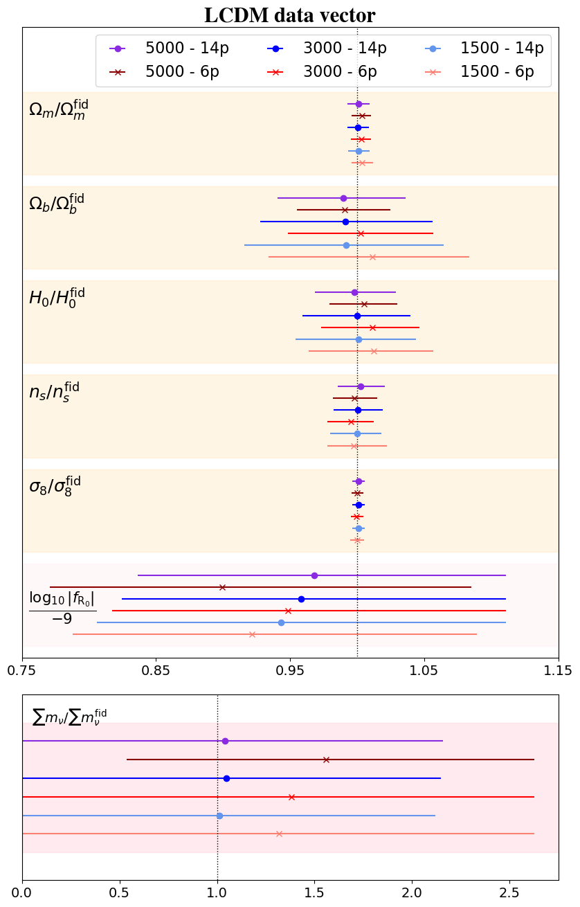
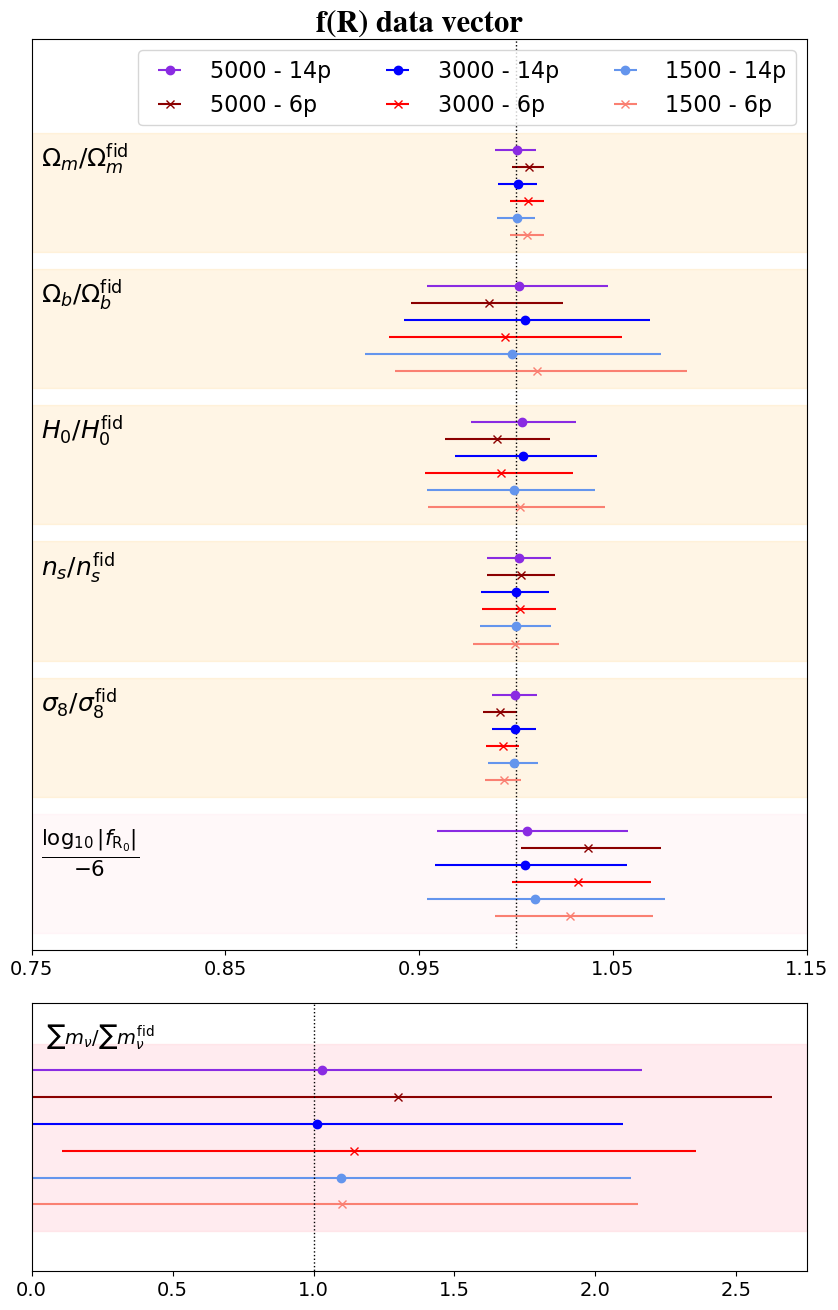
Figure 2: The marginalised means and 2$\sigma$ constraints on the cosmological and beyond-LCDM parameters, normalised to their fiducial values for Scenario A (left) and Scenario B (right), and for all scale cuts and baryonic parameter models.

Table 3: Percent 2$\sigma$ constraints on cosmological and baryonic parameters (at $z=0$) for both Scenarios, both baryonic parameter models and all scale cuts. For Scenario A, we quote the upper $2\sigma$ bound for $\log_{10}|f_{\rm R_{0}}|$ as the fiducial is $f_{\rm R_{0}}=0$. The percent constraints are calculated as $\Delta 2\sigma/\bar{\theta}\times 100\%$, where $\Delta 2\sigma$ is the $2\sigma$ confidence region (upper minus lower) and $\bar{\theta}$ is the marginalised mean parameter value.

	Model	$\ell_{\rm max}$	$\Omega_{\rm m}$	$\Omega_{\rm b}$	$h$	$n_{\rm s}$	$\sigma_{8}$	$\sum m_{\nu}$	$\log_{10}|f_{\rm R_{0}}|$	$\log_{10}M_{\rm c}$	$\mu$	$\theta_{\rm ej}$	$\gamma$	$\delta$	$\eta$	$\eta_{\delta}$
A	14p	1500	1.6	15.0	9.0	3.8	0.9	233.8	-7.25 [upper]	5.8	85.4	66.5	63.5	44.7	146.3	179.2
		3000	1.6	13.0	8.0	3.7	0.9	204.8	-7.42 [upper]	5.2	53.7	52.5	49.3	33.3	104.7	108.5
		5000	1.7	9.6	6.0	3.5	0.9	222.3	-7.53 [upper]	3.2	55.8	33.2	45.6	21.4	79.0	99.6
	6p	1500	1.6	14.8	9.2	4.5	1.0	199.1	-7.09 [upper]	3.0	-	21.8	-	-	-	88.6
		3000	1.5	10.8	7.3	3.5	0.9	190.1	-7.35 [upper]	2.3	-	14.4	-	-	-	85.0
		5000	1.4	7.0	5.0	3.3	0.9	134.1	-6.94 [upper]	1.7	-	9.8	-	-	-	82.4
	fixed	1500	1.1	9.6	7.1	3.1	0.8	225.0	-7.98 [upper]	-	-	-	-	-	-	-
		3000	0.9	5.7	5.5	3.2	0.6	166.1	-8.28 [upper]	-	-	-	-	-	-	-
		5000	0.7	4.8	4.3	3.1	0.5	104.6	-8.37 [upper]	-	-	-	-	-	-	-
B	14p	1500	2.0	15.3	8.7	3.7	2.6	193.6	12.2	6.0	89.8	63.4	73.4	55.0	119.2	147.0
		3000	2.0	12.6	7.3	3.5	2.3	207.0	9.9	5.4	58.4	45.3	53.0	37.3	98.0	104.6
		5000	2.1	9.3	5.4	3.3	2.3	221.7	9.8	3.2	49.4	35.0	43.7	32.0	79.8	102.9
	6p	1500	1.8	14.9	9.1	4.5	1.9	195.8	8.0	2.8	-	24.5	-	-	-	86.8
		3000	1.7	12.1	7.7	3.8	1.8	196.5	6.9	2.0	-	17.3	-	-	-	84.1
		5000	1.6	7.9	5.5	3.5	1.8	229.5	7.0	1.2	-	12.1	-	-	-	83.4
	fixed	1500	1.5	8.3	5.4	3.5	1.6	221.2	4.6	-	-	-	-	-	-	-
		3000	1.4	6.2	4.6	3.3	1.4	179.6	4.1	-	-	-	-	-	-	-
		5000	1.0	5.2	4.1	3.2	1.1	126.8	3.6	-	-	-	-	-	-	-

3 Forecasts for Stage IV surveys

3.1 Setup

Our mock survey configuration has the following Stage IV specifications: sky fraction $f_{\rm sky}=0.4$, number density of galaxies per arcminute squared $n=30\,\mathrm{arcmin}^{-2}$ and shape noise parameter $\sigma_{e}=0.3$. We take 10 equipopulated tomographic bins with galaxies following $n_{\rm i}(z)\sim z^{2}\exp(-(z/z_{0})^{3/2})$ (Smail et al., 1995; Joachimi & Bridle, 2010), with $z_{0}=0.9$. For each redshift bin $i=1,\dots 10$ we include a parameter $D_{z_{\rm i}}$ that shifts the mean of the redshift distribution in the bin (Asgari et al., 2021; Spurio Mancini et al., 2022). We vary these parameters assuming a Gaussian prior $\mathcal{N}(0,10^{-4})$ for each of them, following Spurio Mancini et al. (2022).

We perform MCMC analyses on a set of mock cosmic shear data vectors, adopting the fiducial cosmology and baryonic boost parameters given in Table 1. We then consider two scenarios:

1. The Universe is LCDM ($|f_{\rm R_{0}}|=0$). We aim at checking to what extent Stage IV experiments can constrain $f_{\rm R_{0}}$ and $\sum m_{\nu}$.

2. The Universe is $f(R)$ ($|f_{\rm R_{0}}|=10^{-6}$). We aim at checking to what extent Stage IV experiments can detect $|f_{\rm R_{0}}|>0$.

In all analyses we vary all 5 cosmological parameters as well as $|f_{\rm R_{0}}|$ & $\sum m_{\nu}$. To investigate the importance of the baryon parameters when looking to constrain cosmology and gravity, we perform analyses varying both the $7\times 2$- and $3\times 2$-parameter sets (see subsection 2.2). Note that all fiducial spectra are generated using the $7\times 2$-parameter set. Lastly, to examine the impact that nonlinear scales have on the degeneracies, biases and constraints of the various parameters, we adopt three scale cuts, $\ell_{\rm max}=1500$ (pessimistic), $\ell_{\rm max}=3000$ (realistic) and $\ell_{\rm max}=5000$ (optimistic). The pessimistic case is well within the current capabilities of REACT and available fitting formulae such as HMCODE, as shown in Bose et al. (2020), which is what we employ here. The realistic case is also possibly within the current capabilities of available codes, for example using REACT to construct the boost with the newest version of HMCODE (Mead et al., 2020), and combining with state-of-the-art LCDM emulators such as the Euclid Emulator (Knabenhans et al., 2021). Finally, the optimistic case represents a possible modelling potential given, for example, high quality emulators for the pseudo power spectrum (Giblin et al., 2019). To implement these choices we use 50 $\ell$ bins in the range $[30,5000]$, which for our $\ell_{\rm max}=1500,3000$ runs we cut to multipoles up to the corresponding values. For each setup we assume a simple Gaussian covariance matrix (Joachimi et al., 2007). Note that we leave for future work the inclusion of non Gaussian (Sato & Nishimichi, 2013; Krause & Eifler, 2017) and super sample (Takada & Hu, 2013; Li et al., 2014; Lacasa et al., 2018) contributions (see also a discussion on their possible impact in section 4).

In summary, we study 3 scale cuts and 2 baryonic models for each of the 2 scenarios, giving a total 12 analyses. We vary 33 (25) parameters in total: 5 cosmological $+\sum m_{\nu}$ & $\log_{\rm 10}|f_{\rm R_{0}}|$, 14 (6) baryonic, 2 intrinsic alignment and 10 redshift distribution shift parameters. We sample our posterior distribution using PolyChord (Handley et al., 2015a, b), using 1000 live points to ensure accurate contours despite the large parameter space. A single likelihood evaluation takes approximately 0.7 seconds on a single Intel Xeon E5640 CPU core. PolyChord does not allow one to specify the number of samples as the sampling terminates once a given accuracy threshold is reached. This takes longer for more complex posteriors, i.e. for a larger number of parameters and a larger scale cut. Our longest run, the 14 parameter, $\ell_{\rm max}=5000$, run took approximately one day on 512 cores.

3.2 Results

The $2\sigma$ constraints on all cosmological and baryonic parameters are summarised in Table 3 for all cases considered in this work. We also show the constraints and shifts of the recovered cosmological parameters in Figure 2. Note that $\log_{10}|f_{\rm R_{0}}|$ takes values below the effective LCDM-limit of $-9$ as we emulate down to $-10$. In Appendix A we give the full set of posterior distributions for all parameters except the redshift-dependency parameters of the baryonic effects, which we find to be largely unconstrained. This is provided for both scenarios, all scale cuts and both choices of baryonic parameter sets.

3.2.1 Scenario A

In Figure 3 we show the marginalised 2-dimensional 95% ($2\sigma$) and 68% ($1\sigma$) distributions for the cosmological parameters as well as the beyond-LCDM parameters $\sum m_{\nu}$ and $|f_{\rm R_{0}}|$. We summarise the main findings below and forward the reader to Table 3 for the exact constraints.

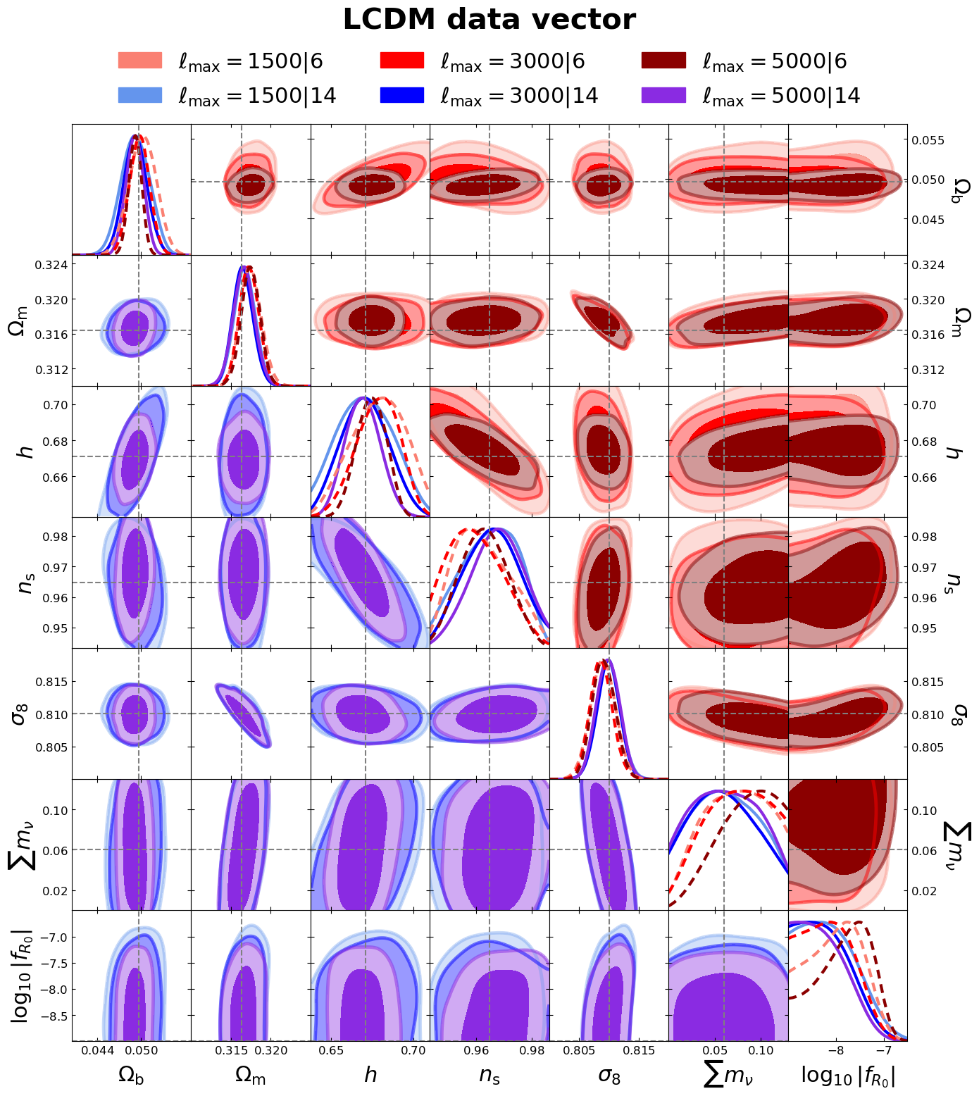
Figure 3: 2-dimensional cosmological parameter posteriors for the $7\times 2$ (bottom-left) and $3\times 2$ (top-right) baryonic parameter models in Scenario A (LCDM data vector). We show the $\ell_{\rm max}=1500,3000,5000$ cases for both baryonic models.

• In the conservative case ($\ell_{\rm max}=1500$) we find that cosmic shear is able to constrain all LCDM cosmological parameters at least at the $\sim 10\%$ level (95 % C.L.), with almost an order of magnitude better constraints on $\Omega_{\mathrm{m}}$ and $\sigma_{8}$. $n_{\mathrm{s}}$ is also better constrained, but to a lesser extent ($3.8\%$).

• The inclusion of scales $1500\leq\ell\leq 5000$ does not significantly improve the base LCDM cosmological parameters, with the most significant improvement being in constraints on $h$ (up to a 6% measurement) and $\Omega_{\mathrm{b}}$ (roughly a factor of 2 with respect to the conservative case).

• Even in the conservative case ($\ell_{\rm max}=1500$) cosmic shear is able to constrain $|f_{\rm R_{0}}|\leq 10^{-7}$ (95 % C.L.), while $\sum m_{\nu}$ remains largely unconstrained.

• The inclusion of scales $1500\leq\ell\leq 5000$ does not significantly improve the constraints on $\sum m_{\nu}$ and $|f_{\rm R_{0}}|$.

• Reducing the number of baryonic degrees of freedom from $7\times 2$ to $3\times 2$ does not notably improve constraints on any parameter nor does it lead to any significant (up to $1\sigma$) biases in the recovered cosmological parameters. We find at most $\sim 1\sigma$ shifts on the $\sum m_{\nu}$ and $|f_{\rm R_{0}}|$ marginalised posteriors in the $\ell_{\rm max}=5000$ case.

These results show that the highly nonlinear scales have only a marginal amount of information on massive neutrinos and modified gravity which is not degenerate with baryonic degrees of freedom. Similarly, the baryonic degrees of freedom dampen the cosmological information one is able to extract from small, nonlinear scales. This was already shown in Copeland et al. (2018). There the authors illustrate how cosmological and dark energy constraints degrade with marginalisation of baryonic effects and that there is little improvement by going to smaller scales. Further, highly consistent results were also found in Bose et al. (2020), where similar poor gains in constraining power on $\log_{10}|f_{\rm R_{0}}|$ was found when including scales $1500\leq\ell\leq 3000$. They do however obtain worse overall constraints compared to ours, by almost half an order of magnitude on $f_{\rm R_{0}}$, despite their analysis not including baryonic degrees of freedom nor massive neutrinos. This is likely due to the difference in setup, as for example we use 10 tomographic bins while they only considered 3.

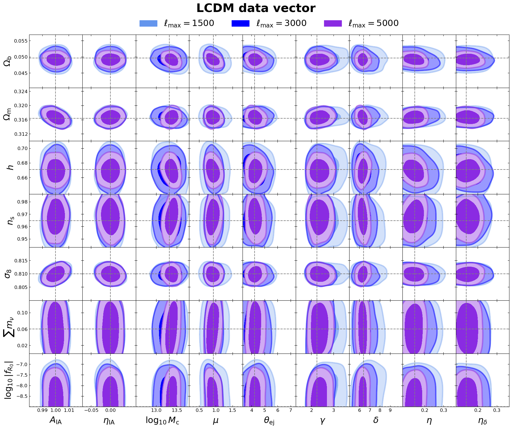
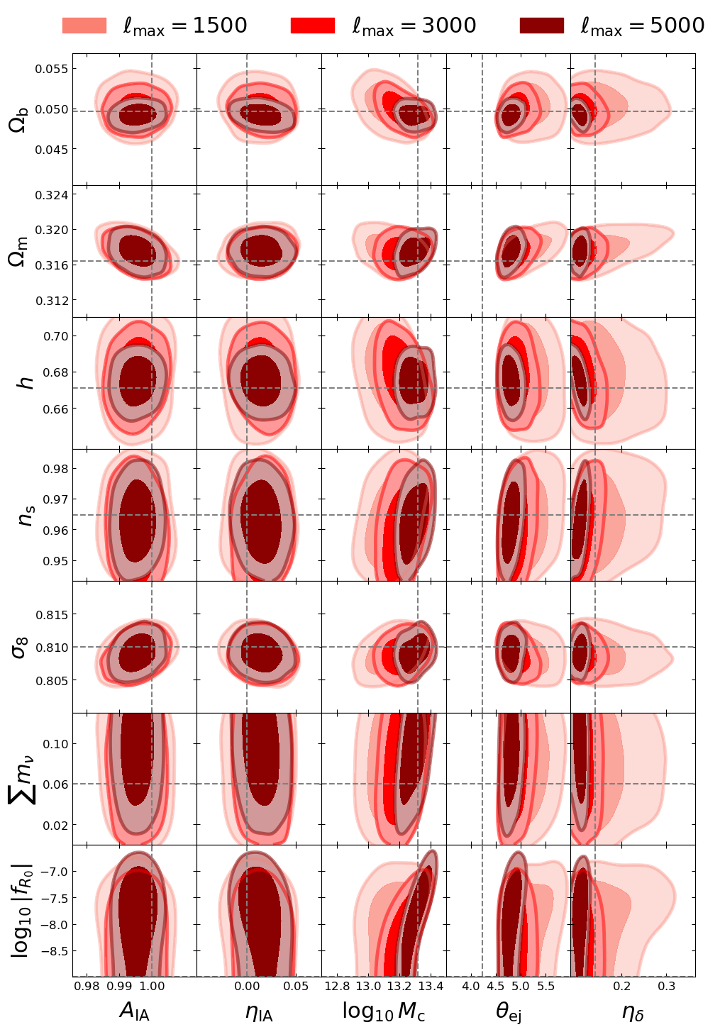
Figure 4: 2-dimensional posteriors between cosmological parameters and baryonic parameters at $z=0$ for the $7\times 2$ (left) and $3\times 2$ (right) parameter models in Scenario A (LCDM data vector). We show the $\ell_{\rm max}=1500,3000,5000$ cases for both baryonic models.

To investigate further the origin of this lack of constraining power on cosmological parameters at highly nonlinear scales, we plot the posteriors for the cosmological, intrinsic alignment and baryonic degrees of freedom. This is shown in Figure 4. It is clear from these plots that much of the information at nonlinear scales is associated with the baryonic degrees of freedom, with all of these parameters seeing significant gains in constraints when moving from $\ell_{\rm max}=1500$ to $\ell_{\rm max}=5000$. This is also clearly seen in Table 3. Notably, in the $7\times 2$ parameter case, there are no large degeneracies between baryonic degrees of freedom and cosmological ones, which supports the lack of improvement in constraining power on cosmological parameters when moving to nonlinear scales. Baryonic parameters are in general less constrained than cosmological parameters, with the exception of $\log_{10}M_{\mathrm{c}}$ which can be constrained down to the $\sim 5$% level even in conservative configurations. However, baryonic parameters are in general more heavily biased, up to $2\sigma$ for $\theta_{\mathrm{ej}}$, when using the reduced model with $3\times 2$ parameters over the one with $7\times 2$ parameters.

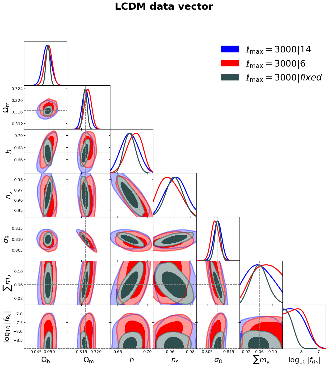
Figure 5: Selected 2-dimensional cosmological parameter posteriors for analyses varying $7\times 2$ (blue), $3\times 2$ (red) and no (green) baryonic parameters in Scenario A (LCDM data vector) using $\ell_{\rm max}=3000$.

In Table 3 we also show the marginalised constraints for Scenario A analyses but with all baryonic degrees of freedom fixed to their fiducial values. As in Schneider et al. (2020a), this represents an ideal situation where baryonic effects are completely known . In Figure 5 we plot the posterior contours for the cosmological parameters in this setup where we assume perfect knowledge of the baryonic parameters, for the realistic configuration $\ell_{\mathrm{max}}=3000$, and we compare the results against those obtained with the same $\ell$-cut, but varying either all of the $7\times 2$ or all of the $3\times 2$ baryonic parameters. We see that knowing the baryonic effects improves constraining power, relative to the $7\times 2$ parameter model, on $\Omega_{m}$, $h$ and $\sum m_{\nu}$ by 50%, and by almost an order of magnitude on $f_{\rm R_{0}}$. Unlike Schneider et al. (2020a) we see little improvement on $n_{s}$, which is likely due to the mild degeneracy of $n_{s}$ with $f_{\rm R_{0}}$ and $\sum m_{\nu}$. As expected, the constraint on $\Omega_{\mathrm{b}}$ is significantly improved, by roughly factor of 2, which just indicates that the baryon fraction is degenerate with baryonic effects.

3.2.2 Scenario B

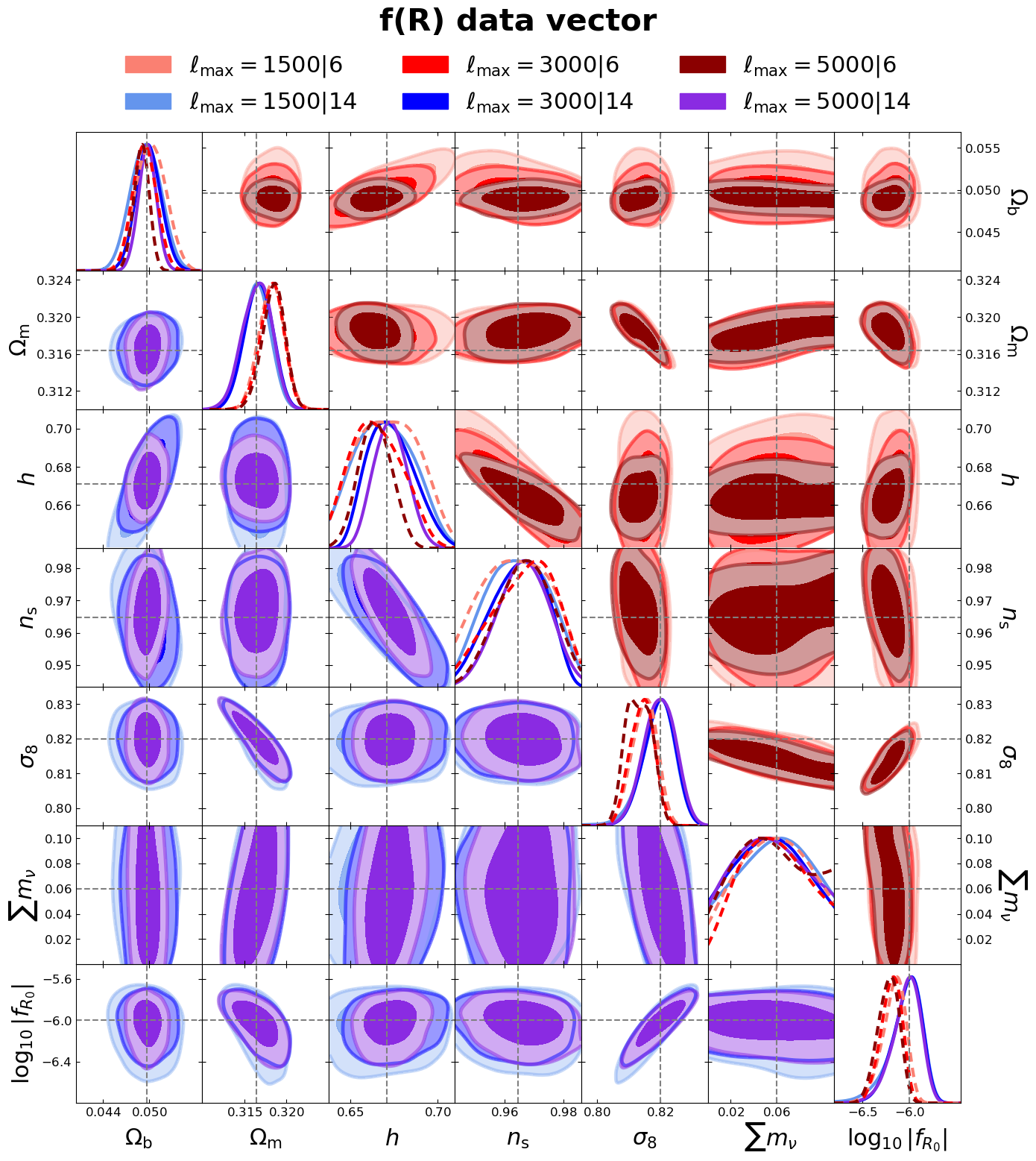
Figure 6: Same as Figure 3 but for Scenario B.

In Figure 6 we show the marginalised 2-dimensional distributions for the cosmological parameters as well as the beyond-LCDM parameters. The main findings are consistent with Scenario A, with marginally worse constraints on $\sigma_{8}$ and $\sum m_{\nu}$. This is driven by the strong degeneracies between $\sigma_{8}$, $|f_{\rm R_{0}}|$ and $\sum m_{\nu}$. At all scales, increasing $\log_{10}|f_{\rm R_{0}}|$ will naturally increase $\sigma_{8}$ as the modification works to enhance power, giving the correlation we see between these parameters. Conversely, massive neutrinos are known to suppress power and so we expect an anti-correlation between $\sum m_{\nu}$ and $\sigma_{8}$.

We note that weak lensing alone is able to provide a clear detection of $f(R)$ gravity, given a modification of $\log_{10}|f_{\rm R_{0}}|=10^{-6}$, even in the presence of massive neutrinos. This detection is not changed notably by including scales $1500\leq\ell\leq 5000$, and is moderately improved by reducing the baryonic parameters. These results are highly consistent with the results of Bose et al. (2020), which performed a similar analysis without massive neutrinos and no baryonic effects. It is clear that even without baryons and massive neutrinos, most constraining power comes from scales $\ell\leq 1500$.

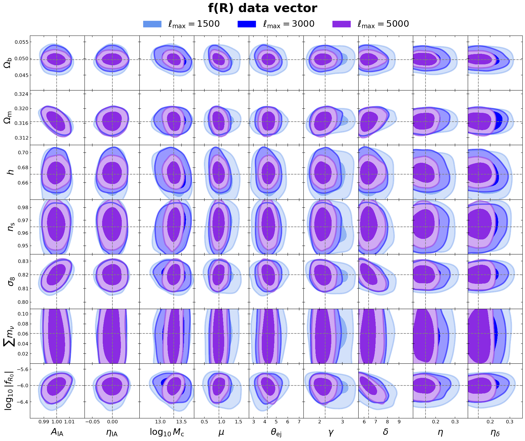
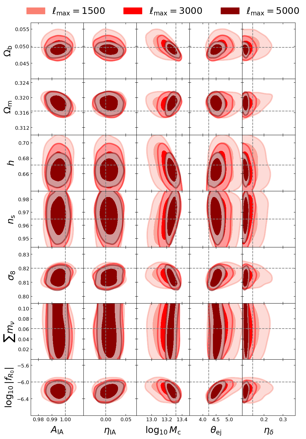
Figure 7: Same as Figure 4 but for Scenario B.

We also show the marginalised posterior distributions between the cosmological and baryonic parameters in Figure 7. This uncovers clear degeneracies between $f(R)$ effects and baryonic physics in the reduced baryonic parameter model, which accounts for the gain in constraining power when moving to very nonlinear scales, which breaks these degeneracies. On the other hand, the full baryonic model does not exhibit such strong degeneracies and we gain less in this case when moving to highly nonlinear scales.

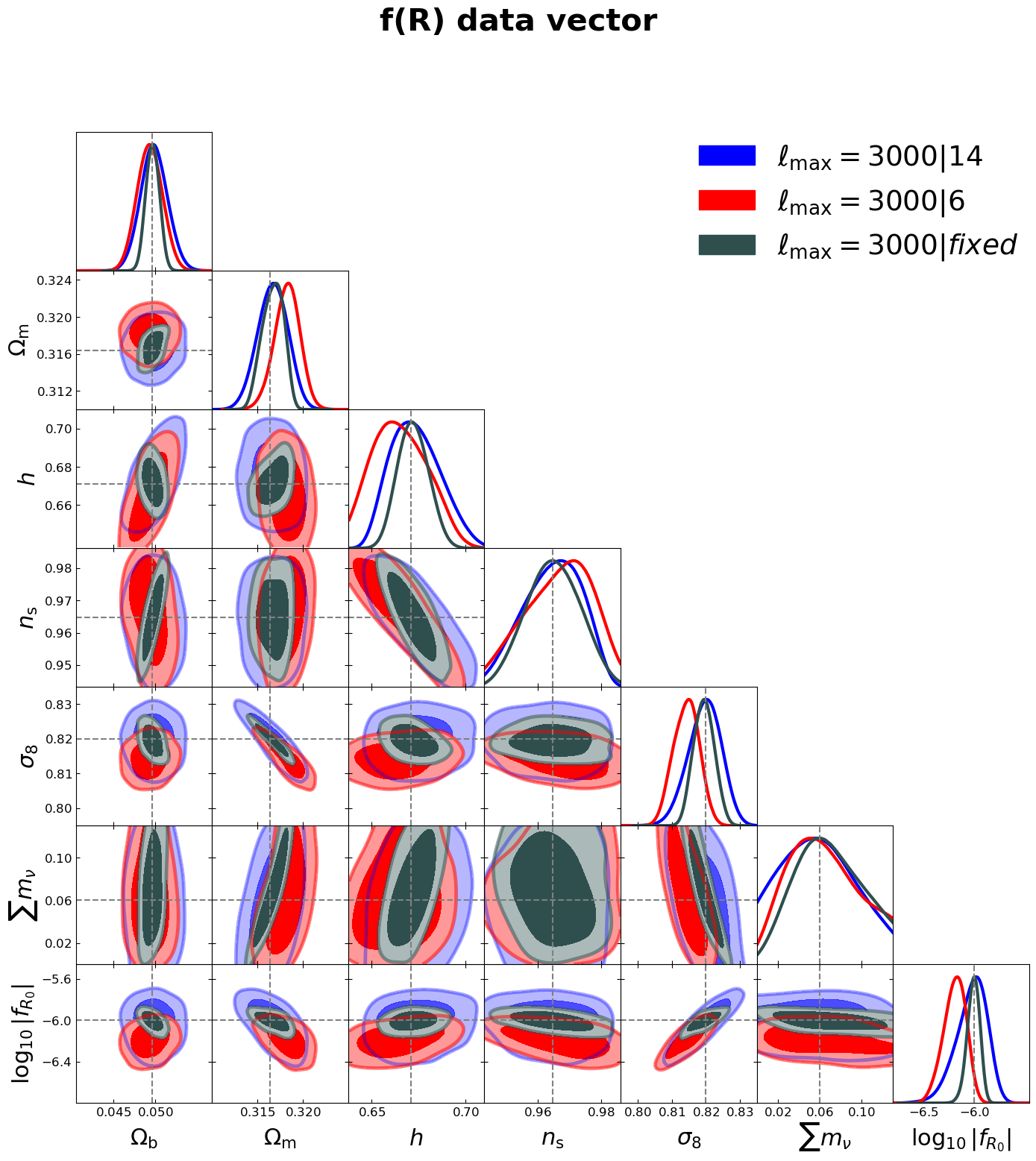
Figure 8: Selected 2-dimensional cosmological parameter posteriors for analyses varying $7\times 2$ (blue), $3\times 2$ (red) and no (green) baryonic parameters in Scenario B (f(R) data vector) using $\ell_{\rm max}=3000$.

In Table 3 we report the expected constraints obtained in the realistic case $\ell_{\mathrm{max}}=3000$ assuming perfect knowledge of the baryonic parameters. In Figure 8 we compare these results against the contours for the $7\times 2$ and $3\times 2$ parameter models. From this comparison we observe that opening up the parameter space for baryonic parameters leads to significantly worse constraints on all cosmological parameters, particularly on $|f_{R_{0}}|$.

4 Conclusions

In this work we have presented a lightening fast pipeline to perform cosmic shear analyses in beyond-LCDM scenarios. To accomplish this we have created an emulator, REACTEMU-FR for the modification to the nonlinear LCDM power spectrum coming from Hu-Sawicki $f(R)$ gravity and massive neutrinos based on halo model reaction predictions. Together with the state-of-the-art baryonic feedback emulator, BCEMU, the pipeline has sufficient accuracy to be applied to Stage IV surveys’ mildly nonlinear data (roughly multipoles $\ell_{\rm max}\leq 1500$). Combining with available tools such as the Euclid Emulator (Knabenhans et al., 2021) would upgrade our pipeline to be safely applied to nonlinear scales, which we roughly define as multipoles $\ell\leq 3000$. Given the development of high quality emulators for the pseudo spectrum (Giblin et al., 2019), a necessary component of the $f(R)$-massive neutrino boost, one could push to even larger multipoles, say $\ell\leq 5000$. We consider all these scale cuts in our paper and denote them as pessimistic, realistic and optimistic cases respectively.

Using our pipeline, we have run a number of mock data analyses using cosmic shear, providing forecasts for forthcoming surveys on modified gravity and massive neutrinos. Our main findings are as follows:

1. Scales between $1500\leq\ell\leq 5000$ offer only mild improvements to constraining power on cosmology, with most power going into constraining non-degenerate baryonic parameters.

2. Using a reduced baryonic parameter set ($3\times 2=6$ instead of $7\times 2=14$) does not impact constraints on any cosmological parameters significantly, but does improve massive neutrino constraints marginally. Further, using this reduced model may lead to significant biases in the baryonic degrees of freedom.

A number of papers have provided similar forecasts in the literature. First, we compare with the LCDM forecasts of Blanchard et al. (2020). We obtain surprisingly consistent constraints on $\Omega_{m}$, $n_{\rm s}$ and $\sigma_{8}$, but significantly better constraints on $\Omega_{b}$ and $h$, of factors of 4 and 2 respectively. The differences we observe may be caused by our higher redshift range (they stop at $z=2.5$) and our slightly higher sky fraction. Further, our nonlinear prescriptions are also very different. We make use of HMCODE while they employ halofit, and we include baryonic feedback via BCEMU while they do not consider feedback at all. These differences to the absolute power can have significant impacts on the constraining power (Martinelli et al., 2021).

In any case, it is expected that the inclusion of cross-correlations with galaxy clustering, and the full $3\times 2$pt analysis, will give far better constraints on all cosmological parameters (Blanchard et al., 2020). Future surveys will also offer constraints on baryonic physics (Huang et al., 2021) which can be combined with other probes of baryonic physics. As we have shown, this will lead to improved constraints on massive neutrinos and $f(R)$ gravity, besides being interesting in its own right. However, we also note that our analysis has optimistically assumed a Gaussian covariance, ignoring super-sample contributions which in all likelihood will degrade the overall constraining power. A detailed investigation of this aspect is left for future work, as is the inclusion of optimal weighting schemes for physical scales (e.g. Bernardeau et al., 2014; Taylor et al., 2018a; Deshpande et al., 2020).

Moving on to studies of $f(R)$ gravity, in Bose et al. (2020) they do not include baryonic or massive neutrino physics and have slightly different survey specifications, including far fewer tomographic bins (3 bins vs our 10 bins). Despite these differences, we find similar contributing constraining power when including multipoles between $1500\leq\ell\leq 3000$ for both the LCDM fiducial and the $f(R)$ fiducial mock data analyses as well as similar overall constraints on $f(R)$.

Similarly, Harnois-Déraps et al. (2022) do not include massive neutrinos nor baryonic effects, and have significant differences in the survey specifications and setup. Notably they use 5 tomographic bins up to $z=3$, a quarter of our sky fraction, only consider auto-tomographic bins and have a restricted prior on $f_{\rm R_{0}}$. Given this, they naturally report weaker overall constraints in their full MCMC analyses. Interestingly, their Fisher analysis finds that the constraints on $f_{\rm R_{0}}$ will improve when including highly nonlinear scales, in contrast to what we find. We remind the reader though that they do not consider baryons, which also dampen the $f(R)$ constraints as well as their analysis having fixed the other cosmological parameters, and so representing an absolutely ideal scenario.

More similar to our analysis is that of Schneider et al. (2020a); Schneider et al. (2020b) which include a similar baryonic model as used in this work, but without redshift evolution, and including massive neutrinos and $f(R)$ gravity, albeit separately and using different theoretical prescriptions. They also use a different nonlinear power spectrum prescription, as well as only include 3 tomographic bins in the range $0.1\leq z\leq 1.5$, and take $\ell_{\rm max}=4000$. The authors report significantly weaker constraints on cosmological, $f(R)$ and neutrino mass parameters. The number of tomographic bins may lead to our improved constraints, particularly on cosmological parameters. Schneider et al. (2020b) do find almost 2 orders of magnitude worse constraints on $f_{\rm R_{0}}$ than Bose et al. (2020) but include baryonic degrees of freedom which significantly worsen the constraints. On the other hand, we also include baryonic degrees of freedom and obtain $\sim$2.5 orders of magnitude better constraints.

Another possibility could be the difference in tomographic binning and maximum redshift, which would contribute highly to these improved constraints as $f_{\rm R_{0}}$, $\sigma_{8}$ and $\sum m_{\nu}$ all have different redshift evolutions. The power spectrum becomes highly insensitive to $f_{\rm R_{0}}$ at early times (it being a late-time modification), breaking degeneracies with $\sigma_{8}$ and $\sum m_{\nu}$. This means more redshift information will improve constraints, particularly high redshift information which was also pointed out in Harnois-Déraps et al. (2022), where they showed that most Fisher information on modified gravity is contained in the highest redshift bin. Finally, it was shown in Taylor et al. (2018b) that a large number of bins are needed to capture the high-redshift information when using equipopulated binning.

Lastly, a recent analysis (Aricò et al., 2023) of the Dark Energy Survey year 3 data including baryons, massive neutrinos and the same intrinsic alignment model employed here has shown consistent constraints on the $S_{8}$ parameter after considering they employ a sky fraction that is roughly 4 times less than that employed here. Their constraints on $\Omega_{m}$ are still significantly worse than ours, and the forecast of Blanchard et al. (2020) for example. We also employ 6 times the number density of their analysis, which will vastly improve constraining power on small scales. Survey specifications and the full power of Stage IV make such comparisons difficult, but we deem these results to be well within our expectations. It is also worth noting that this analysis (Aricò et al., 2023) was possible due to improvements in the prior ranges of the BACCO emulator. Priors can be informative and it is important to have accurate nonlinear modelling across a wide parameter space (see Carrilho et al., 2023, for example), making REACT emulation an easy and viable means of performing data analyses for beyond-LCDM scenarios.

We conclude by noting that such a high dimensional parameter space analysis is both necessary and challenging when looking to optimise reliable information extraction from Stage IV surveys. It is also worthwhile as nonlinear scales can provide considerable information on interesting extensions to LCDM. Our analyses has focused on a minimal extension to LCDM, and serves as a ‘proof of principle’ and ‘proof of worth’ for the tools used in this paper, notably COSMOPOWER and REACT, which we combined to provide REACTEMU-FR. One key goal of forthcoming Stage IV surveys is to provide clues for solving the looming theoretical issues of Dark Energy and, even more broadly, the cosmological constant problem (see Bernardo et al., 2023, for a recent review on modified gravity solutions). Thus, pipelines able to accurately model comprehensive extensions to LCDM becomes an absolute necessity. Such extensions have already been proposed (see Bose et al., 2022, for example), but include a number of new degrees of freedom, making the need for emulation even more clear, as is the development of fast inference pipelines based on gradient-based sampling techniques (see e.g. Ruiz-Zapatero et al., 2023; Campagne et al., 2023; Piras & Spurio Mancini, 2023). It is straightforward to include existing models of gravity and dark energy into this emulation framework. It is also the goal of ongoing work to integrate these and perform similar tests as part of necessary preparation for the data releases of the largest galaxy surveys to date.

Data Availability

REACTEMU-FR is publicly available github.

Appendix A Full posteriors

In this appendix we present the full 2-dimensional marginalised posteriors for all analyses, with the exception of the baryonic feedback redshift-dependency parameters, which we have found to be largely prior dominated.

In Figure 9 we show the results for the $7\times 2$ baryonic parameter model, both when considering a fiducial LCDM data vector and $f(R)$ data vector (Scenarios A & B respectively in the main text). All scale cuts are also shown. Similarly, in Figure 10 we show the results for the reduced $3\times 2$ baryonic parameter model.

These plots visually highlight the vast parameter space that one needs to probe in order to comprehensively account for all known physics, and probe minimal extensions to LCDM. This space can foreseeably increase when looking to move deeper into the nonlinear regime or when wishing to probe more general deviations to LCDM.

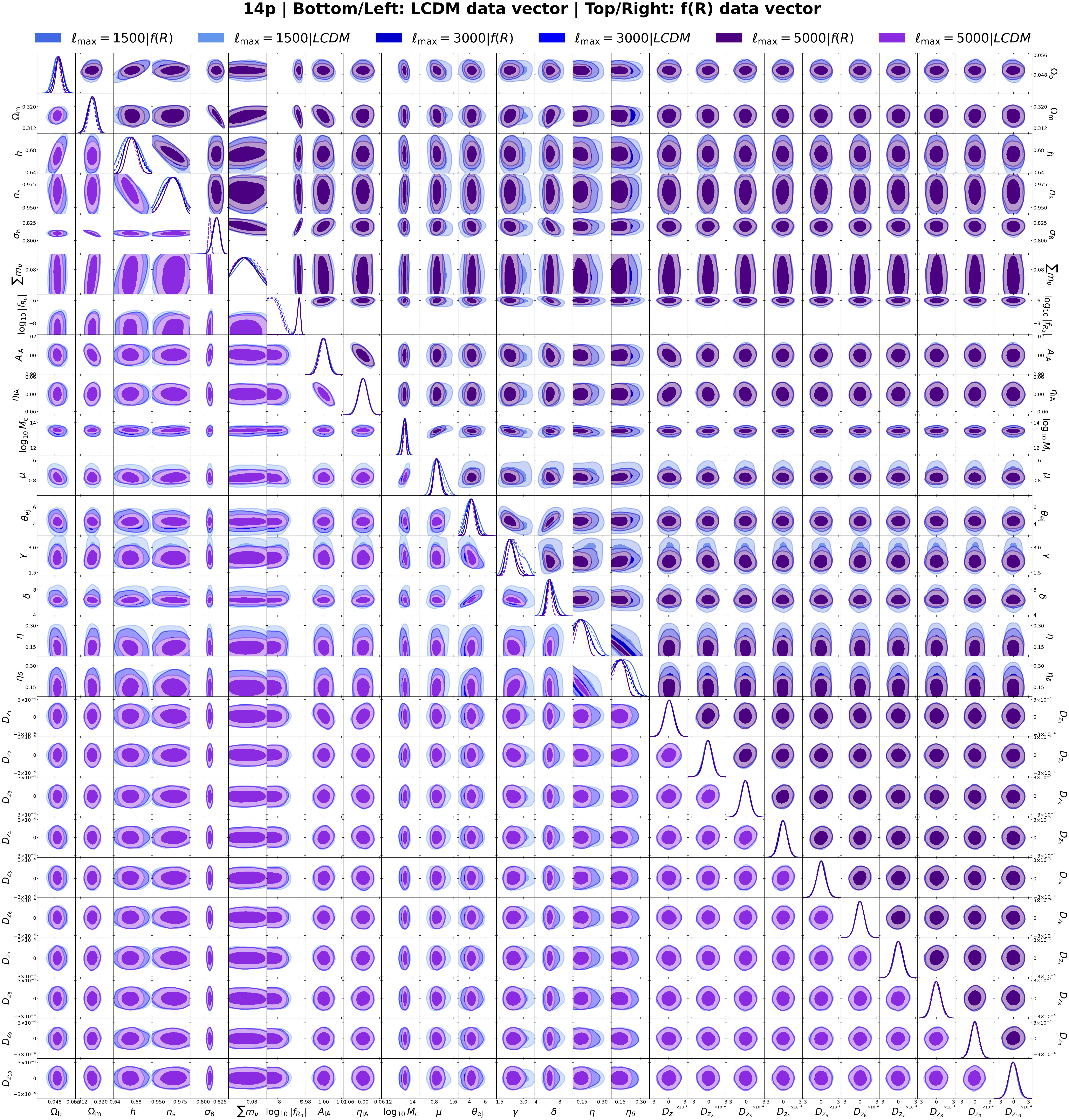
Figure 9: Full set of marginalised 2-dimensional posterior distributions for the $7\times 2$ baryonic parameter model. We show all scale cuts as well as the case where we fit to a LCDM fiducial data vector (bottom left) and $f(R)$ fiducial data vector (top right).

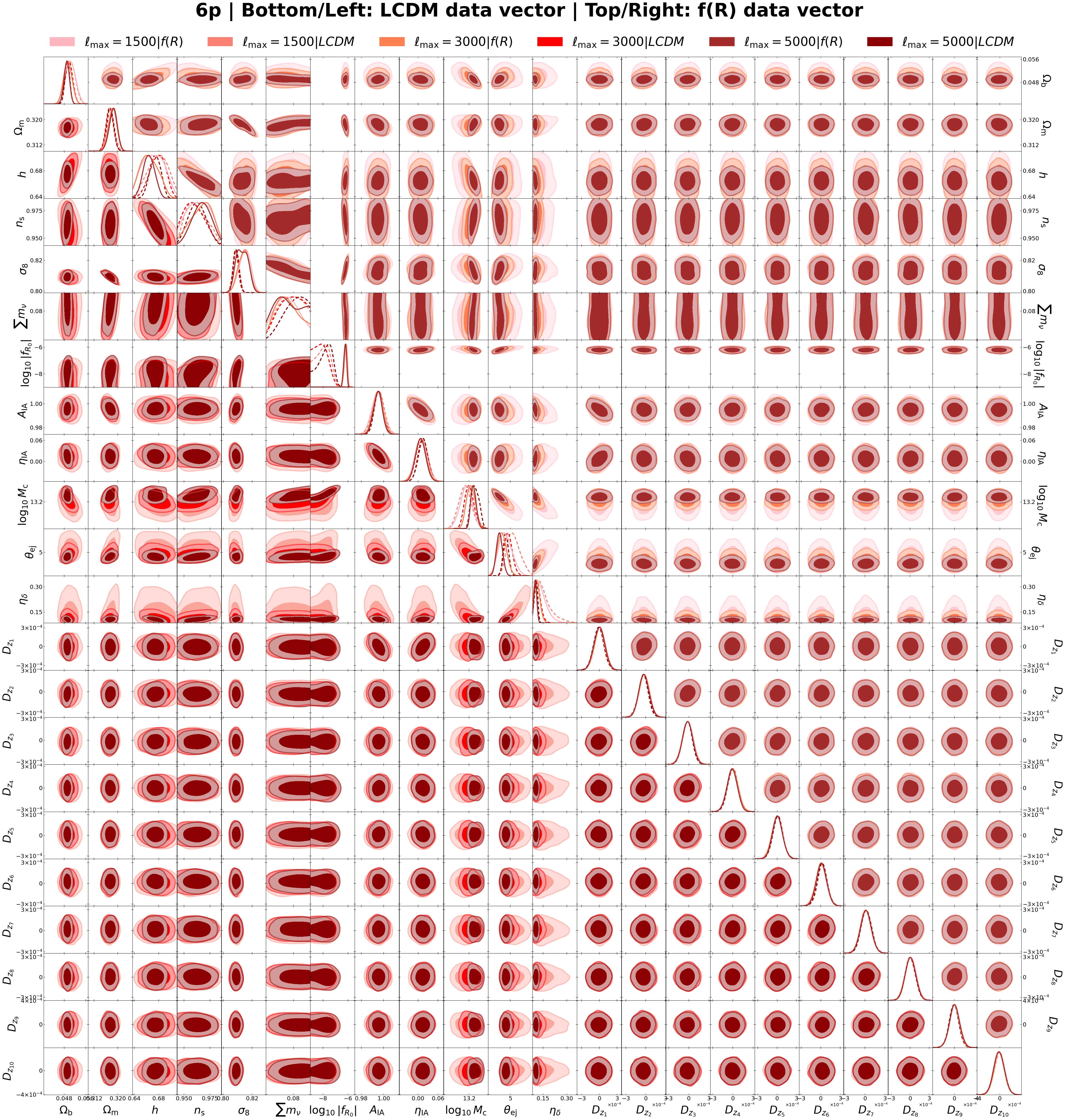
Figure 10: Same as Figure 9 but for the $3\times 2$ baryonic parameter model case.

References

- Adamek et al. (2022) Adamek J., et al., 2022, Euclid: Modelling massive neutrinos in cosmology – a code comparison (arXiv:2211.12457)
- Aghanim et al. (2020) Aghanim N., et al., 2020, Astron. Astrophys., 641, A6
- Ahmed et al. (2004) Ahmed S. N., et al., 2004, Phys. Rev. Lett., 92, 181301
- Aker et al. (2022) Aker M., et al., 2022, Nature Phys., 18, 160
- Amendola et al. (2018) Amendola L., et al., 2018, Living Rev. Rel., 21, 2
- Angulo et al. (2021) Angulo R. E., Zennaro M., Contreras S., Aricò G., Pellejero-Ibañez M., Stücker J., 2021, Mon. Not. Roy. Astron. Soc., 507, 5869
- Aricò et al. (2021) Aricò G., Angulo R. E., Contreras S., Ondaro-Mallea L., Pellejero-Ibañez M., Zennaro M., 2021, Mon. Not. Roy. Astron. Soc., 506, 4070
- Aricò et al. (2023) Aricò G., Angulo R. E., Zennaro M., Contreras S., Chen A., Hernández-Monteagudo C., 2023, DES Y3 cosmic shear down to small scales: constraints on cosmology and baryons (arXiv:2303.05537)
- Arnold et al. (2021) Arnold C., Li B., Giblin B., Harnois-Déraps J., Cai Y.-C., 2021, (arXiv:2109.04984)
- Asgari et al. (2021) Asgari M., et al., 2021, Astronomy & Astrophysics, 645, A104
- Asgari et al. (2023) Asgari M., Mead A. J., Heymans C., 2023, The halo model for cosmology: a pedagogical review (arXiv:2303.08752)
- Bartelmann & Schneider (2001) Bartelmann M., Schneider P., 2001, Phys. Rep., 340, 291
- Bernardeau et al. (2014) Bernardeau F., Nishimichi T., Taruya A., 2014, Monthly Notices of the Royal Astronomical Society, 445, 1526
- Bernardo et al. (2023) Bernardo H., Bose B., Franzmann G., Hagstotz S., He Y., Litsa A., Niedermann F., 2023, Universe, 9, 63
- Blanchard et al. (2020) Blanchard A., et al., 2020, Astron. Astrophys., 642, A191
- Bose et al. (2020) Bose B., Cataneo M., Tröster T., Xia Q., Heymans C., Lombriser L., 2020, Mon. Not. Roy. Astron. Soc., 498, 4650
- Bose et al. (2021) Bose B., et al., 2021, Mon. Not. Roy. Astron. Soc., 508, 2479
- Bose et al. (2022) Bose B., Tsedrik M., Kennedy J., Lombriser L., Pourtsidou A., Taylor A., 2022, (arXiv:2210.01094)
- Brax et al. (2021) Brax P., Casas S., Desmond H., Elder B., 2021, Universe, 8, 11
- Bridle & King (2007) Bridle S., King L., 2007, New J. Phys., 9, 444
- Campagne et al. (2023) Campagne J.-E., et al., 2023, The Open Journal of Astrophysics, 6
- Carrilho et al. (2022) Carrilho P., Carrion K., Bose B., Pourtsidou A., Hidalgo J. C., Lombriser L., Baldi M., 2022, Mon. Not. Roy. Astron. Soc., 512, 3691
- Carrilho et al. (2023) Carrilho P., Moretti C., Pourtsidou A., 2023, JCAP, 01, 028
- Cataneo et al. (2015) Cataneo M., et al., 2015, Phys. Rev. D, 92, 044009
- Cataneo et al. (2019) Cataneo M., Lombriser L., Heymans C., Mead A., Barreira A., Bose S., Li B., 2019, Mon. Not. Roy. Astron. Soc., 488, 2121
- Copeland et al. (2018) Copeland D., Taylor A., Hall A., 2018, Mon. Not. Roy. Astron. Soc., 480, 2247
- Deshpande et al. (2020) Deshpande A. C., Taylor P. L., Kitching T. D., 2020, Phys. Rev. D, 102, 083535
- Desmond & Ferreira (2020) Desmond H., Ferreira P. G., 2020, Phys. Rev. D, 102, 104060
- Fukuda et al. (1998) Fukuda Y., et al., 1998, Phys. Rev. Lett., 81, 1158
- Giblin et al. (2019) Giblin B., Cataneo M., Moews B., Heymans C., 2019, Mon. Not. Roy. Astron. Soc., 490, 4826
- Giri & Schneider (2021) Giri S. K., Schneider A., 2021, JCAP, 12, 046
- Handley et al. (2015a) Handley W. J., Hobson M. P., Lasenby A. N., 2015a, Monthly Notices of the Royal Astronomical Society: Letters, 450, L61
- Handley et al. (2015b) Handley W. J., Hobson M. P., Lasenby A. N., 2015b, Monthly Notices of the Royal Astronomical Society, 453, 4385
- Harnois-Déraps et al. (2022) Harnois-Déraps J., Hernandez-Aguayo C., Cuesta-Lazaro C., Arnold C., Li B., Davies C. T., Cai Y.-C., 2022, (arXiv:2211.05779)
- Hu & Sawicki (2007) Hu W., Sawicki I., 2007, Phys.Rev., D76, 064004
- Huang et al. (2021) Huang H.-J., et al., 2021, Mon. Not. Roy. Astron. Soc., 502, 6010
- Ivezić et al. (2019) Ivezić v., et al., 2019, Astrophys. J., 873, 111
- Joachimi & Bridle (2010) Joachimi B., Bridle S. L., 2010, A&A, 523, A1
- Joachimi et al. (2007) Joachimi B., Schneider P., Eifler T., 2007, Astronomy & Astrophysics, 477, 43
- Kaiser (1998) Kaiser N., 1998, The Astrophysical Journal, 498, 26
- Kilbinger (2015) Kilbinger M., 2015, Reports on Progress in Physics, 78, 086901
- Kilbinger et al. (2017) Kilbinger M., et al., 2017, Monthly Notices of the Royal Astronomical Society, 472, 2126
- Kitching et al. (2017) Kitching T. D., Alsing J., Heavens A. F., Jimenez R., McEwen J. D., Verde L., 2017, Monthly Notices of the Royal Astronomical Society, 469, 2737
- Knabenhans et al. (2019) Knabenhans M., et al., 2019, Mon. Not. Roy. Astron. Soc., 484, 5509
- Knabenhans et al. (2021) Knabenhans M., et al., 2021, Mon. Not. Roy. Astron. Soc., 505, 2840
- Koyama (2016) Koyama K., 2016, Reports on Progress in Physics, 79, 046902
- Krause & Eifler (2017) Krause E., Eifler T., 2017, Monthly Notices of the Royal Astronomical Society, 470, 2100
- Lacasa et al. (2018) Lacasa F., Lima M., Aguena M., 2018, A&A, 611, A83
- Laureijs et al. (2011) Laureijs R., et al., 2011, (arXiv:1110.3193)
- Lawrence et al. (2017) Lawrence E., et al., 2017, Astrophys. J., 847, 50
- Lesgourgues & Pastor (2006) Lesgourgues J., Pastor S., 2006, Phys. Rept., 429, 307
- Lewis (2019) Lewis A., 2019, (arXiv:1910.13970)
- Li et al. (2014) Li Y., Hu W., Takada M., 2014, Physical Review D, 89
- LoVerde & Afshordi (2008) LoVerde M., Afshordi N., 2008, Phys. Rev. D, 78, 123506
- Lombriser (2014) Lombriser L., 2014, Annalen Phys., 526, 259
- Martinelli et al. (2021) Martinelli M., et al., 2021, Astron. Astrophys., 649, A100
- Mead (2017) Mead A., 2017, Mon. Not. Roy. Astron. Soc., 464, 1282
- Mead et al. (2016) Mead A., Heymans C., Lombriser L., Peacock J., Steele O., Winther H., 2016, Mon. Not. Roy. Astron. Soc., 459, 1468
- Mead et al. (2020) Mead A., Brieden S., Tröster T., Heymans C., 2020, Mon. Not. Roy. Astron. Soc.
- Merloni et al. (2012) Merloni A., et al., 2012, eROSITA Science Book: Mapping the Structure of the Energetic Universe (arXiv:1209.3114)
- Parimbelli et al. (2022) Parimbelli G., Carbone C., Bel J., Bose B., Calabrese M., Carella E., Zennaro M., 2022, JCAP, 11, 041
- Piras & Spurio Mancini (2023) Piras D., Spurio Mancini A., 2023, The Open Journal of Astrophysics, 6
- Ramachandra et al. (2021) Ramachandra N., Valogiannis G., Ishak M., Heitmann K., 2021, Phys. Rev. D, 103, 123525
- Ruiz-Zapatero et al. (2023) Ruiz-Zapatero J., Hadzhiyska B., Alonso D., Ferreira P. G., García-García C., Mootoovaloo A., 2023, Monthly Notices of the Royal Astronomical Society
- Samuroff et al. (2021) Samuroff S., Mandelbaum R., Blazek J., 2021, Mon. Not. Roy. Astron. Soc., 508, 637
- Sato & Nishimichi (2013) Sato M., Nishimichi T., 2013, Physical Review D, 87
- Schneider et al. (2020a) Schneider A., Stoira N., Refregier A., Weiss A. J., Knabenhans M., Stadel J., Teyssier R., 2020a, JCAP, 04, 019
- Schneider et al. (2020b) Schneider A., et al., 2020b, JCAP, 04, 020
- Semboloni et al. (2011) Semboloni E., Hoekstra H., Schaye J., van Daalen M. P., McCarthy I. J., 2011, Mon. Not. Roy. Astron. Soc., 417, 2020
- Smail et al. (1995) Smail I., Ellis R. S., Fitchett M. J., Edge A. C., 1995, Monthly Notices of the Royal Astronomical Society, 273, 277
- Spergel et al. (2015) Spergel D., et al., 2015, arXiv e-prints, p. arXiv:1503.03757
- Spurio Mancini & Pourtsidou (2022) Spurio Mancini A., Pourtsidou A., 2022, Mon. Not. Roy. Astron. Soc., 512, L44
- Spurio Mancini et al. (2022) Spurio Mancini A., Piras D., Alsing J., Joachimi B., Hobson M. P., 2022, Mon. Not. Roy. Astron. Soc., 511, 1771
- Srinivasan et al. (2021) Srinivasan S., Thomas D. B., Pace F., Battye R., 2021, JCAP, 06, 016
- Takada & Hu (2013) Takada M., Hu W., 2013, Physical Review D, 87
- Takahashi et al. (2012) Takahashi R., Sato M., Nishimichi T., Taruya A., Oguri M., 2012, Astrophys. J., 761, 152
- Taylor et al. (2018a) Taylor P. L., Bernardeau F., Kitching T. D., 2018a, Phys. Rev. D, 98, 083514
- Taylor et al. (2018b) Taylor P. L., Kitching T. D., McEwen J. D., 2018b, Phys. Rev. D, 98, 043532
- Winther et al. (2019) Winther H., Casas S., Baldi M., Koyama K., Li B., Lombriser L., Zhao G.-B., 2019, Phys. Rev. D, 100, 123540
- Wright et al. (2019) Wright B. S., Koyama K., Winther H. A., Zhao G.-B., 2019, JCAP, 06, 040
- Zhao (2014) Zhao G.-B., 2014, Astrophys. J. Suppl., 211, 23