Magnetic Catalysis in Holographic Model with Two Types of Anisotropy for Heavy Quarks

Abstract

In our previous paper [1] we have constructed a twice anisotropic five-dimensional holographic model supported by Einstein-dilaton-three-Maxwell action that reproduced some essential features of the “heavy quarks” model. However, that model did not describe the magnetic catalysis (MC) phenomena expected from lattice results for the QGP made up from heavy quarks. In this paper we fill this gap and construct the model that improves the previous one. It keeps typical properties of the heavy quarks phase diagram, and meanwhile possesses the MC. The deformation of previous model includes the modification of the “heavy quarks” warp factor and the coupling function for the Maxwell field providing the non-trivial chemical potential.

1 Introduction

Quantum chromodynamics (QCD) is a theory that describes strong interactions between subatomic particles such as quarks and gluons. Complete description of the QCD phase diagram in a parameter space with temperature, chemical potential, quark masses, anisotropy, magnetic field etc. is a challenging and very important task in high energy physics. Standard methods to do calculations in QCD such as perturbation no longer work for the strongly coupled regime of this theory, while the lattice theory has problems with non-zero chemical potential calculations. Hence, to understand physics of the strongly coupled quark–gluon plasma (QGP) produced in heavy ion collisions (HIC) at RHIC and at the LHC, and future experiments, we need a non-perturbative approach [2, 3, 4].

According to the results of the experiments with relativistic HIC, it is believed that a very strong magnetic field, $eB\sim 0.3$ GeV², is created in the early stages of the collision [5, 6, 7, 8]. Therefore, magnetic field is an important parameter characterizing the QCD phase diagram expected from the experiments with relativistic HIC [9, 10, 11]. Studying QCD in the background of magnetic field has received much attention recent years, among other things, because of such an interesting phenomena as chiral magnetic effect [12, 13], magnetic catalysis (MC) [14, 15], inverse magnetic catalysis (IMC) [16, 17], as well as the early Universe physics [18, 19] and dense neutron stars [20]. Therefore, investigation of the magnetic field effect on the QCD features and in particular its phase diagram is very interesting and crucial for better understanding of the QCD. Besides, such an investigation has been considered via lattice calculations [21, 22, 23, 24]. For more information and detailed reviews the interested reader is referred to [15, 10] and references therein. In particular, many holographic QCD models have been developed to investigate the effect of magnetic field on the characteristics of QCD [25, 26, 27, 28, 29, 30, 31, 32, 33, 34, 35, 36, 37, 38, 39, 40, 41, 42, 43].

The enhancement effect of the phase transition temperature under the magnetic field increasing is known as MC phenomenon, the opposite effect is called IMC. Lattice calculations show that for small chemical potential there is a substantial influence of the magnetic field on the QCD phase diagram structure. This influence essentially depends on the quark mass: for small quark mass (light quarks) IMC takes place, meanwhile for large mass (heavy quarks) MC occurs. In this context note that lattice calculations predict different types of phase transitions even for small chemical potential and zero magnetic field – we have a crossover for light quarks, and a first-order phase transition for heavy quarks. The holographic QCD models for heavy and light quarks constructed in [44, 45, 46, 48, 47, 37] reproduce these phase diagram features at small chemical potential and predict new interesting phenomena for finite chemical potential, in particular, the locations of the critical end points. In our previous papers [49], see also [29], where the light quark holographic model with non-zero magnetic field is investigated, it has been shown that IMC takes place. Our paper [1] shows that the heavy quark holographic model [45] still has IMC, not MC, that contradicts with lattice zero chemical potential calculation. This indicates that one has to modify the heavy quark holographic model [1].

In the current paper we fill this gap and construct a heavy quark model that improves the previous one [45, 50, 1]. The main goal of the improvements is to get the MC phenomenon in holographic description of the heavy quarks’ first order phase transition scenario with external magnetic field keeping typical properties of the heavy quarks phase diagram. For this purpose we can consider additional $z^{4}$- [51, 52, 53] or/and $z^{5}$-terms [54, 55] into the exponent warp factor. In particular, within this holographic model we show that $z^{4}$-term allows to produce the MC phenomenon required.

As we have emphasized in the previous papers [56, 45, 46], there is a reason to introduce one more parameter characterizing the QCD phase diagram – an anisotropy parameter $\nu$. Non-central HIC produces anisotropic QGP, and the isotropisation time is estimated as $1$–$5$ fm/$c\sim 10^{-24}$ s [57]. Anisotropic holographic models have been used to study QGP in [58, 59, 60, 61, 62, 56, 67, 64, 65, 63, 66]. One of the main purposes to consider anisotropic models is to describe the experimental energy dependence of total multiplicity of particles created in HIC [68]. In [56] it has been shown that the choice of the primary anisotropy parameter value about $\nu=4.5$ reproduces the energy dependence of total multiplicity [68]. Note that isotropic models could not reproduce it (for more details see [56] and references therein). In addition, it is very interesting to know how the primary (spatial) anisotropy can affect the QCD phase transition temperature. Note also that there is another type of anisotropy due to magnetic field and its effect on the QCD phase diagram is a subject of interest.

In this work we set up a twice anisotropic “heavy quarks” model. In fact, we consider 5-dim Einstein-Maxwell-dilaton action with three Maxwell fields: the first Maxwell field sets up finite non-zero chemical potential in the gauge theory, the second Maxwell field provides the primary spatial anisotropy to reproduce the multiplicity dependence on energy, and the 3-rd Maxwell field provides another anisotropy that originates from magnetic field in the gauge theory. We use an anisotropic metric as an ansatz to solve Einstein equations and the field equations self-consistently. The central question of the current investigation is the form of the warp factor able to provide the MC phenomenon within the constructed holographic model. This our consideration shows a phenomenological character of the bottom-up holographic models [69, 75, 77, 78, 79, 81, 82, 76, 83, 4, 84, 85, 86, 87, 47, 88, 89, 90, 91, 92, 93, 98, 94, 45, 50, 1, 46, 97, 49, 80, 53, 54, 95, 96, 73, 74, 72, 71, 70], that is different from the top-down holographic models [99, 100, 101, 102, 103].

This paper is organized as follows. In section 2 we present a 5-dim holographic model to describe a hot dense anisotropic QCD in the magnetic field background. In section 3 we introduce an appropriate warp factor able to produce MC phenomenon in this holographic model and obtain the first order phase transition for the model parameters. In section 4 we review our main results. This work in complemented with Appendix A where we solve EOMs, Appendix B where we present expressions for the blackening function derivatives, gauge coupling functions and dilaton potential, and Appendix C where we consider the relation of our setting with the setting [53] explicitly.

2 Holographic Model with three Maxwell Fields

Let us take the Lagrangian in Einstein frame used in [1]:

$${\cal L}=\sqrt{-g}\left[R-\cfrac{f_{0}(\phi)}{4}\,F_{0}^{2}-\cfrac{f_{1}(\phi)}{4}\,F_{1}^{2}-\cfrac{f_{3}(\phi)}{4}\,F_{3}^{2}-\cfrac{1}{2}\,\partial_{\mu}\phi\,\partial^{\mu}\phi-V(\phi)\right],$$ (2.1)

where $R$ is Ricci scalar, $\phi$ is the scalar field, $f_{0}(\phi)$, $f_{1}(\phi)$ and $f_{3}(\phi)$ are the coupling functions associated with stresses $F_{0}$, $F_{1}$ and $F_{3}$ of Maxwell fields, and $V(\phi)$ is the scalar field potential. In this paper we considered $F_{0}$, $F_{1}$ and $F_{3}$ as first, second and third Maxwell fields, respectively.

Varying Lagrangian (2.1) over the metric we get Einstein equations of motion (EOMs):

$$G_{\mu\nu}=T_{\mu\nu},$$ (2.2)

where

$$G_{\mu\nu}=R_{\mu\nu}-\cfrac{1}{2}\,g_{\mu\nu}R,\qquad\cfrac{\delta S_{m}}{\delta g^{\mu\nu}}=\frac{1}{2}\,T_{\mu\nu}\sqrt{-g},$$ (2.3)

and varying over the fields gives the fields equations

$$-\nabla_{\mu}\nabla^{\mu}\phi+V^{\prime}(\phi)+\!\!\sum_{i=0,1,3}\!\!\cfrac{f_{i}^{\prime}(\phi)}{4}\,F_{(i)}^{2}=0,$$ (2.4)

$$\partial_{\mu}\left(\sqrt{-g}\,f_{i}\,F_{(i)}^{\mu\nu}\right)=0.$$ (2.5)

Let us take the metric ansatz in the following form:

$$ds^{2}=\cfrac{L^{2}}{z^{2}}\ \mathfrak{b}(z)\left[-\,g(z)\,dt^{2}+dx_{1}^{2}+\left(\cfrac{z}{L}\right)^{2-\frac{2}{\nu}}dx_{2}^{2}+e^{c_{B}z^{2}}\left(\cfrac{z}{L}\right)^{2-\frac{2}{\nu}}dx_{3}^{2}+\cfrac{dz^{2}}{g(z)}\right]\!,$$ (2.6)

$$\mathfrak{b}(z)=e^{2{\cal A}(z)},$$

and for matter fields

$$\phi=\phi(z),\quad\,$$ (2.7)

$$\begin{split}F_{0}\,-\,\mbox{electric ansatz }\,\,A_{0}&=A_{t}(z),\quad A_{i}=0,\,\,i=1,2,3,4,\\ F_{k}\,-\,\mbox{magnetic ansatz}\quad F_{1}&=q_{1}\,dx^{2}\wedge dx^{3},\quad F_{3}=q_{3}\,dx^{1}\wedge dx^{2}\,.\end{split}$$ (2.8)

In (2.6) $L$ is the AdS-radius, $\mathfrak{b}(z)$ is the warp factor set by ${\cal A}(z)$, $g(z)$ is the blackening function, $\nu$ is the parameter of primary anisotropy caused by non-symmetry of heavy-ion collision (HIC), and $c_{B}$ is the coefficient of secondary anisotropy related to the magnetic field $F_{3}$. Choice of ${\cal A}(z)$ determines the heavy/light quarks description of the model. In previous works we considered ${\cal A}(z)=-\,cz^{2}/4$ for heavy quarks [45, 50, 1] and ${\cal A}(z)=-\,a\,\ln(bz^{2}+1)$ for light quarks [46, 49]. In (2.8) $q_{1}$ and $q_{3}$ are constant “charges”.

The explicit form of the EOM (2.3–2.5) with ansatz (2.7)–(2.8) is given in Appendix (A.12–A.18). Investigation of their self-consistency shows that there is one dependent equation in the system and all other equations are independent. Thus, system (A.12–A.18) is self-consistent and the dilaton field equation (A.12) serves as a constraint.

It is important to note that the coupling function $f_{0}$ is defined from the requirement to reproduce the Regge trajectories. Functions $f_{1}$ and $f_{3}$ are obtained from the EOM, and we find that they are different (see Appendices A and B for more details). If we take $f_{0}=f_{1}=f_{3}$, then we cannot construct a solution of EOM within our ansatz.

Note that while solving equations of motions we do not actually get $f_{0}(\phi)$, $f_{1}(\phi)$, $f_{3}(\phi)$ and $V(\phi)$ dependencies, but obtain $f_{0}(\phi(z))=f_{0}(z)$, $f_{1}(\phi(z))=f_{1}(z)$, $f_{3}(\phi(z))=f_{3}(z)$ and $V(\phi(z))=V(z)$. The reason is that $\phi(z)$-expression is rather complicated, so the analytic expression for the inverse function $z=z(\phi)$ can’t be written down. There still remains the possibility to get this function via approximation, but such a result can be useful for a limited number of aspects only because of lack of accuracy.

3 Magnetic Catalysis for Heavy Quarks

Our goal is to generalize solution [1] to get magnetic catalysis effect on the heavy quarks version of the phase diagram. For this purpose we choose the deformation of the warp factor from [1] again. This factor has been used in [51, 52] to reproduce Cornell potential and in [53] also to get magnetic catalysis effect.

3.1 Solution and thermodynamics for ${\cal A}(z)=-\,cz^{2}/4\,-pz^{4}$

Our strategy to solve the EOMs presented in Appendix A with the factor ${\cal A}(z)=-\,cz^{2}/4\,-pz^{4}$ is the same as in [1] and [46]. Subtracting (A.17) from (A.16) we get the expression for the third Maxwell field’s coupling function

$$f_{3}=2\left(\cfrac{L}{z}\right)^{\frac{2}{\nu}}\mathfrak{b}g\ \cfrac{c_{B}z}{q_{3}^{2}}\left(\cfrac{g^{\prime}}{g}+\cfrac{3\mathfrak{b}^{\prime}}{2\mathfrak{b}}-\cfrac{2}{\nu z}+c_{B}z\right)$$ (3.1)

and rewrite equation (A.14) as

$$g^{\prime\prime}+g^{\prime}\left(\cfrac{3\mathfrak{b}^{\prime}}{2\mathfrak{b}}-\cfrac{\nu+2}{\nu z}-c_{B}z\right)-2g\left(\cfrac{3\mathfrak{b}^{\prime}}{2\mathfrak{b}}-\cfrac{2}{\nu z}+c_{B}z\right)c_{B}z-\left(\cfrac{z}{L}\right)^{2}\cfrac{f_{0}(A_{t}^{\prime})^{2}}{\mathfrak{b}}=0.$$ (3.2)

To derive the exact solutions we just need to specify the warp factor:

$$\mathfrak{b}(z)=e^{2{\cal A}(z)}=e^{-\,cz^{2}/2\,-\,2pz^{4}}.$$ (3.3)

Following [95, 48, 53] we take $c=4R_{gg}/3$, $R_{gg}=1.16$, $p=0.273$ (this choice is dictated by the Regge spectra and lattice QCD fitting) and solve system (A.12)–(A.18) with usual boundary conditions

$$A_{t}(0)=\mu,\quad A_{t}(z_{h})=0,$$ (3.4)

$$g(0)=1,\quad g(z_{h})=0,$$ (3.5)

$$\phi(z_{0})=0,$$ (3.6)

where $z_{0}$ serves to fit the string tension behavior [46].

Equation (A.13) with (C.8) gives

$$A_{t}(z)=\mu\,\cfrac{e^{(2R_{gg}+c_{B}(q_{3}-1))\frac{z^{2}}{2}}-e^{(2R_{gg}+c_{B}(q_{3}-1))\frac{z_{h}^{2}}{2}}}{1-e^{(2R_{gg}+c_{B}(q_{3}-1))\frac{z_{h}^{2}}{2}}}=\mu\left(1-\cfrac{1-{e^{(2R_{gg}+c_{B}(q_{3}-1))\frac{z^{2}}{2}}}}{1-{e^{(2R_{gg}+c_{B}(q_{3}-1))\frac{z_{h}^{2}}{2}}}}\right).$$ (3.7)

For $q_{3}=1$ and $c_{B}=C$ the result (3.7) coincides with the expressions (2.27) and (2.31) in [53]:

$$A_{t}(z)=\mu\left(1-\cfrac{1-{e^{R_{gg}z^{2}}}}{1-{e^{R_{gg}z_{h}^{2}}}}\right).$$ (3.8)

Density is the coefficient in $A_{t}$ expansion:

$$A_{t}(z)=\mu-\rho\,z^{2}+\dots\ \Longrightarrow\ \rho=-\,\cfrac{\mu\bigl{(}2R_{gg}+c_{B}(q_{3}-1)\bigr{)}}{2\left(1-e^{(2R_{gg}+c_{B}(q_{3}-1))\frac{z_{h}^{2}}{2}}\right)}.$$ (3.9)

The electric potential $A_{t}(z)$ and density $\rho(z_{h})/\mu$ in logarithmic scale are depicted in Fig.1 in panels A and B, respectively.

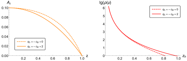
A                                                                 B

Figure 1: Electric potential $A_{t}(z)$ (A) and density $\rho(z_{h})/\mu$ in logarithmic scale (B) for the “heavy quarks” case with (solid lines) and without (dashed lines) magnetic field, $q_{3}=-\,c_{B}=0,\,2$ (B); $R_{gg}=1.16$; $[z]^{-1}=$ GeV.

Equation (3.2) with (C.8) and (3.7) gives

$$g(z)=e^{c_{B}z^{2}}\left[1-\cfrac{I_{1}(z)}{I_{1}(z_{h})}+\cfrac{\mu^{2}\bigl{(}2R_{gg}+c_{B}(q_{3}-1)\bigr{)}I_{2}(z)}{L^{2}\left(1-e^{(2R_{gg}+c_{B}(q_{3}-1))\frac{z_{h}^{2}}{2}}\right)^{2}}\left(1-\cfrac{I_{1}(z)}{I_{1}(z_{h})}\,\cfrac{I_{2}(z_{h})}{I_{2}(z)}\right)\right],$$ (3.10)

$$I_{1}(z)=\int_{0}^{z}e^{\left(2R_{gg}-3c_{B}\right)\frac{\xi^{2}}{2}+3p\xi^{4}}\xi^{1+\frac{2}{\nu}}\,d\xi,\quad I_{2}(z)=\int_{0}^{z}e^{\bigl{(}2R_{gg}+c_{B}\left(\frac{q_{3}}{2}-2\right)\bigr{)}\xi^{2}+3p\xi^{4}}\xi^{1+\frac{2}{\nu}}\,d\xi.$$ (3.11)

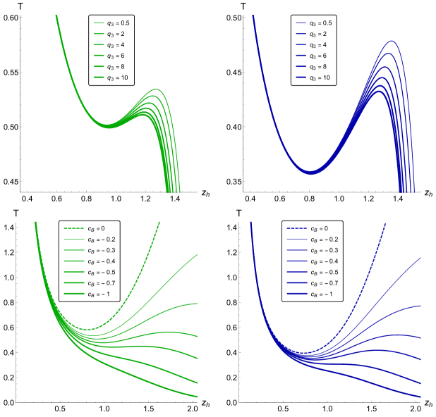
A                                                                 B

Figure 2: Temperature $T(z_{h})$ for different $q_{3}$, $c_{B}=-\,0.3$ and $\mu=\,0.2$ (1-st line) and for different $c_{B}$, $q_{3}=1$ and $\mu=\,0$ (2-nd line); $\nu=1$ (A) and $\nu=4.5$ (B); $R_{gg}=1.16$, $p=0.273$; $[T]=[z_{h}]^{-1}=$ GeV.

We use the following formulas of temperature and entropy:

$$T=\cfrac{\sqrt{{g_{tt}}^{\prime}\,{g^{zz}}^{\prime}}}{4\pi}\,\Bigl{|}_{z=z_{h}}=\cfrac{\sqrt{{g_{00}}^{\prime}\,{g^{44}}^{\prime}}}{4\pi}\,\Bigl{|}_{z=z_{h}},$$ (3.12)

$$s=\cfrac{\sqrt{g_{xx}\,g_{y_{1}y_{1}}\,g_{y_{2}y_{2}}}}{4}\,\Bigl{|}_{z=z_{h}}=\cfrac{\sqrt{g_{11}\,g_{22}\,g_{33}}}{4}\,\Bigl{|}_{z=z_{h}}.$$ (3.13)

For the metric (2.6) and the warp factor (3.3) temperature and entropy can be written as:

$$T=\cfrac{|g^{\prime}|}{4\pi}\,\Biggl{|}_{z=z_{h}}=\Biggl{|}-\,\cfrac{e^{(2R_{gg}-c_{B})\frac{z_{h}^{2}}{2}+3pz_{h}^{4}}\,z_{h}^{1+\frac{2}{\nu}}}{4\pi\,I_{1}(z_{h})}\,\times$$

$$\begin{split}&\times\left[1-\cfrac{\mu^{2}\bigl{(}2R_{gg}+c_{B}(q_{3}-1)\bigr{)}\left(e^{(2R_{gg}+c_{B}(q_{3}-1))\frac{z_{h}^{2}}{2}}I_{1}(z_{h})-I_{2}(z_{h})\right)}{L^{2}\left(1-e^{(2R_{gg}+c_{B}(q_{3}-1))\frac{z_{h}^{2}}{2}}\right)^{2}}\right]\Biggr{|},\\ s&=\cfrac{1}{4}\left(\cfrac{L}{z_{h}}\right)^{1+\frac{2}{\nu}}e^{-(2R_{gg}-c_{B})\frac{z_{h}^{2}}{2}-3pz_{h}^{4}}.\end{split}$$ (3.14)

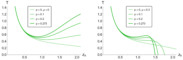
A                                                                 B

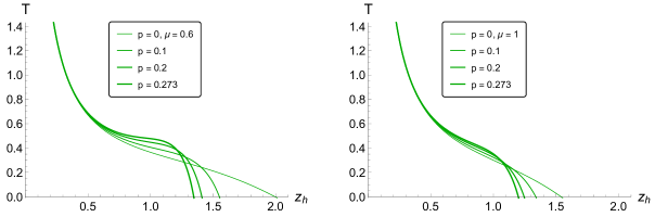
C                                                                 D

Figure 3: Temperature $T(z_{h})$ for different $p$, $\mu=0$ (A), $\mu=0.3$ (B), $\mu=0.6$ (C), $\mu=1$ (D); $\nu=1$, $q_{3}=-\,c_{B}=0.2$, $R_{gg}=1.16$; $[T]=[z_{h}]^{-1}=$ GeV.

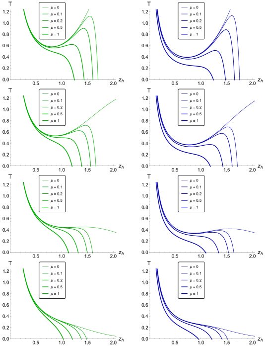
A                                                          B

Figure 4: Temperature $T(z_{h})$ for different $\mu$, $q_{3}=-\,c_{B}=0$ (1-st line), $q_{3}=-\,c_{B}=0.2$ (2-nd line), $q_{3}=-\,c_{B}=0.5$ (3-rd line) and $q_{3}=-\,c_{B}=1$ (4-th line); $\nu=1$ (A) and $\nu=4.5$ (B); $R_{gg}=1.16$, $p=0.273$; $[T]=[z_{h}]^{-1}=$ GeV.

In Fig.2 (first line) we see that magnetic “charge” $q_{3}$ affects the temperature function for the fixed magnetic coefficient $c_{B}$ and non-zero chemical potential $\mu$ values independently from primary anisotropy. For zero chemical potential temperature obviously has no dependence on $q_{3}$ at all, see eq. (3.12). At fixed $c_{B}$ increasing $q_{3}$ decreases the phase transition temperature and evenually makes it monotonic (Fig.2, second line) independently from primary anisotropy as well. All this leads to the idea used in other works to associate the magnetic “charge” with the magnetic coefficient $q_{3}=-\,c_{B}$.

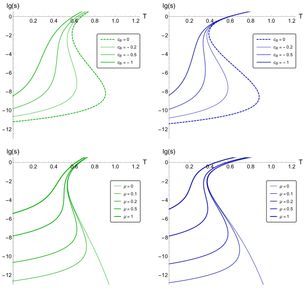
A                                                                 B

Figure 5: Entropy $s(T)$ in logarithmic scale for different $q_{3}=-\,c_{B}$, $\mu=0.2$ (1-st line) and for different $\mu$, $q_{3}=-\,c_{B}=0.2$ (2-nd line); $\nu=1$ (A) and $\nu=4.5$ (B); $R_{gg}=1.16$, $p=0.273$; $[T]$ = GeV.

To understand the role of $pz^{4}$-term in the warp factor let’s consider the temperature behavior for $p=0,\,0.1,\,0.2,\,0.273$ (Fig.3). Earlier in [1] we obtained a hypersensitivity of the background phase transition from the magnetic field: for $c_{B}\sim-\,0.01$ (for $\nu=1$) it fully degenerated. Non-zero $p$ makes the background phase transition in the magnetic field more stable, allowing it to achieve more realistic values (in Fig.3 $q_{3}=-\,c_{B}=0.2$).

In Fig.4 temperature function for different chemical potential values and $p=0.273$ in presented. Magnetic field amplification makes three-valued behavior of $z_{h}(T)$ to become monotonic and lowers the local minimum temperature. Entropy has usual behavior (Fig.5) and the inverse magnetic catalysis can be expected again. To make this sure let us consider a free energy function

$$F=-\int s\,dT=\int_{z_{h}}^{\infty}s\,T^{\prime}dz.$$ (3.15)

Note that for non-zero chemical potential we should integrate to second horizon $z_{h_{2}}$ and for $\mu=0$ we have $z_{h_{2}}=\infty$.

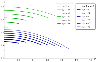
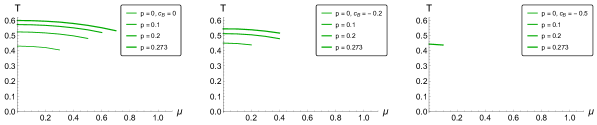
Figure 6: Phase diagram for $\nu=1$ (green lines) and $\nu=4.5$ (blue lines) for $q_{B}=-\,c_{B}$; $R_{gg}=1.16$, $p=0.273$; $[T]=[\mu]=$ GeV.

A                                         B                                         C

Figure 7: Phase diagram for different $p$, $q_{B}=-\,c_{B}=0$ (A), $q_{B}=-\,c_{B}=0.2$ (B), $q_{B}=-\,c_{B}=0.5$ (C); $\nu=1$, $R_{gg}=1.16$, $p=0.273$.

The result for the first order (background) black hole-black hole (BB) phase transition or Hawking-Page-like (HP) phase transition originating from the free energy is presented in Fig.7 and confirms the inverse magnetic catalysis effect. As to the $pz^{4}$-term effect, in Fig.7 we can clearly see that larger $p$-value prevents the background phase transition degeneracy with the magnetic field amplification.

Thus our choice of (3.3) as a warp factor to deform the metric did not possess the MC phenomenon although could lead to good results for IMC. In the next section we consider a new warp factor to produce the proper result for MC phenomenon.

3.2 Solution for ${\cal A}(z)=-\,cz^{2}/4\,-(p-c_{B}q_{3})z^{4}$

In search for the MC phenomenon we considered a corrected version of our new warp factor. Let us remind that varying Lagrangian (2.1) over the metric (2.6) we get the same equations of motion (A.12–A.18) for different fields. Using the new warp factor

$$\mathfrak{b}(z)=e^{2{\cal A}(z)}=e^{-\,cz^{2}/2\,-\,2(p-c_{B}\,q_{3})z^{4}},$$ (3.16)

where $c=4R_{gg}/3$, $R_{gg}=1.16$, $p=0.273$, one can solve system of EOMs (A.12–A.18) with the same boundary conditions (3.4–3.6).

To possess the linear Regge trajectories for the meson mass spectra in our model, in comparison with [53], we considered the kinetic function (C.8) and the new warp factor (3.16). Then, at $T=\mu=B=0$ one can produce linear mass spectrum $m_{n}^{2}=4R_{gg}n$, in such a way that the parameter $R_{gg}$ can be fitted by Regge spectra of meson, such as $J/\psi$. Note also that the parameters $R_{gg}$ and $p$ can be fixed for the zero magnetic field with $R_{gg}=1.16$ and $p=0.273$ [95, 48].

3.2.1 Blackening function

For the corrected factor (3.16) the EOM on the gauge field $A_{t}(z)$ is the same as before and has the same solution (3.7). Therefore, the equation (3.2) with (C.8), (3.7) and the corrected warp factor (3.16) gives

$$g(z)=e^{c_{B}z^{2}}\left[1-\cfrac{\tilde{I}_{1}(z)}{\tilde{I}_{1}(z_{h})}+\cfrac{\mu^{2}\bigl{(}2R_{gg}+c_{B}(q_{3}-1)\bigr{)}\tilde{I}_{2}(z)}{L^{2}\left(1-e^{(2R_{gg}+c_{B}(q_{3}-1))\frac{z_{h}^{2}}{2}}\right)^{2}}\left(1-\cfrac{\tilde{I}_{1}(z)}{\tilde{I}_{1}(z_{h})}\,\cfrac{\tilde{I}_{2}(z_{h})}{\tilde{I}_{2}(z)}\right)\right],$$ (3.17)

$$\tilde{I}_{1}(z)=\int_{0}^{z}e^{\left(2R_{gg}-3c_{B}\right)\frac{\xi^{2}}{2}+3(p-c_{B}\,q_{3})\xi^{4}}\xi^{1+\frac{2}{\nu}}\,d\xi,\qquad\$$ (3.18)

$$\tilde{I}_{2}(z)=\int_{0}^{z}e^{\bigl{(}2R_{gg}+c_{B}\left(\frac{q_{3}}{2}-2\right)\bigr{)}\xi^{2}+3(p-c_{B}\,q_{3})\xi^{4}}\xi^{1+\frac{2}{\nu}}\,d\xi.$$ (3.19)

The behavior of the blackening function $g$ in terms of the holographic coordinate $z$ for different values of the magnetic coefficient $c_{B}$ and different primary anisotropy background, i.e. $\nu=1$ (green lines) and $\nu=4.5$ (blue lines), normalized to the horizon $z_{h}=1$, is depicted in Fig.8.A. Here blackening function is monotonic, and larger values of magnetic coefficient $c_{B}$ correspond to lower $g$ values both in isotropic and anisotropic background. But comparing isotropic and anisotropic backgrounds we see that at $0<|c_{B}|<0.3$ the blackening function gets lower values for $\nu=4.5$ than for $\nu=1$, while at $0.3<|c_{B}|<1$ it is not sensible to changes in primary anisotropies.

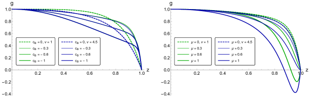
A                                                                 B

Figure 8: The blackening function $g(z)$ for different $c_{B}$ and $\nu$, $\mu=0$ (A) and for different $\mu$ and $\nu$, $c_{B}=-\,0.2$ (B); $\nu=1$ (green lines) and $\nu=4.5$ (blue lines); $R_{gg}=1.16$, $p=0.273$, $q_{3}=5$, $z_{h}=1$; $[z]^{-1}=$ GeV.

The effect of chemical potential on the blackening function for different primary anisotropies of the background is demonstrated in Fig.8.B. Larger $\mu$ decreases the blackening function value in both isotropic and anisotropic background cases. But, for the fixed chemical potential the blackening function value is smaller in the background with larger primary anisotropy. Note also that for large chemical potential values one has to deal with the second black hole horizon.

3.2.2 Scalar field

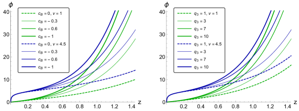
A                                                                 B

Figure 9: The dilaton field $\phi(z)$ for different $c_{B}$, $q_{3}=5$ (A) and different $q_{3}$, $c_{B}=-\,0.5$ (B); $\nu=1$ (green lines) and $\nu=4.5$ (blue lines); $R_{gg}=1.16$, $p=0.273$, $z_{0}=0.001$; $[z]^{-1}=$ GeV.

The scalar, i.e. dilaton field $\phi$ can be derived from equation (A.15) with the boundary condition (3.6) imposed

$$\begin{split}\phi(z)&=\int_{z_{0}}^{z}\Bigl{[}-\,4+\frac{2}{3}\,\nu\Biggl{(}6+3\,(c_{B}\,(2-3\nu)+6R_{gg}\nu)\,\xi^{2}+\bigl{(}-\,3\,c_{B}(c_{B}+60\,q_{3})\,+\\ &+4(45\,p+R_{gg}^{2})\bigr{)}\,\nu\xi^{4}+48R_{gg}(p-c_{B}\,q_{3})\,\nu\xi^{6}+144\,(p-c_{B}\,q_{3})^{2}\,\nu\xi^{8}\Bigr{)}\Biggr{]}^{\frac{1}{2}}\,\frac{d\xi}{\nu\xi}.\end{split}$$ (3.20)

Expanding the integrand of the dilaton field we have $\phi(z)\sim\int_{z_{0}}^{z}\sqrt{\nu-1}\,d\xi/\xi$. Therefore, the dilaton field has no divergency at $z_{0}=0$ on the primary isotropic background $\nu=1$, while on anisotropic background a logarithmic divergency exists. It is important to note that we generalize the boundary condition for the dilaton field as $\phi(z_{0})=0$ [46, 96], where $z_{0}$ can be some function of $z_{h}$. The fact is that the scalar field boundary conditions can affect the temperature dependence of the string tension, i.e. the coefficient of the linear term of the Cornell potential. The string tension should decrease with the temperature growth and become zero at the confinement/deconfinement phase transition [109, 110, 111]. To preserve this feature and also avoid divergences in anisotropic backgrounds we considered the dilaton boundary condition as $\phi(z_{0})=0$. For special cases one can consider $z_{0}=0$ [48] and $z_{0}=z_{h}$ [45].

Fig.9 shows that the scalar field is a monotonically increasing function of the holographic coordinate $z$ both in primary isotropic and anisotropic cases, i.e. for $\nu=1$ and $\nu=4.5$, but larger primary anisotropy shifts the dilaton curve up to larger $\phi$-values. Larger absolute value of the magnetic coefficient $c_{B}$ and larger magnetic charge $q_{3}$ make $\phi(z)$ to grow faster (Fig.9.A and B respectively).

3.2.3 Coupling function $f_{3}$

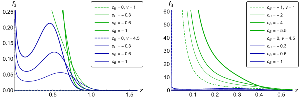
A                                                                 B

Figure 10: The coupling function $f_{3}(z)$ for different $c_{B}$, $\mu=0$ (A) and for different $c_{B}$, $\mu=0.2$ (B); $\nu=1$ (green lines) and $\nu=4.5$ (blue lines); $z_{h}=1.5$, $R_{gg}=1.16$, $p=0.273$, $q_{3}=5$; $[z]^{-1}=$ GeV.

The function $f_{3}$ that describes the coupling between the third Maxwell field $F_{3}$ and the dilaton field $\phi$ is still calculated by the expression (3.1). The detailed formula obtained by substituting the blackening function, it’s derivative and the corrected warp factor (3.16) is presented in Appendix B. For zero magnetic coefficient $c_{B}=0$ the coupling function $f_{3}$ obviously equals zero. It’s behavior depending on the holographic direction $z$ is plotted in Fig.10. We see that for zero chemical potential $\mu=0$ it is positive and preserves the NEC both in isotropic $\nu=1$ and primary anisotropic $\nu=4.5$ backgrounds (Fig.10.A). However in the isotropic background we see the decreasing monotonic behavior of $f_{3}(z)$, while in the anisotropic background it demonstrates a multivalued behavior with a local minimum and a local maximum. Note also that for larger magnetic coefficient (larger $c_{B}$ absolute values) $f_{3}$ is positive not everywhere beyond the fixed horizon $z_{h}$, therefore we need to choose appropriate parameters in our theory and in particular the correct value for the second horizon to have positive value for coupling function $f_{3}$ (see the Fig.10.B for the second horizon $z_{h_{2}}=0.55$ for $\nu=1$ and $z_{h_{2}}=0.45$ for $\nu=4.5$).

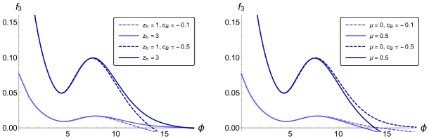
A                                                                 B

Figure 11: The coupling function $f_{3}(\phi)$ different $z_{h}$ and $c_{B}$, $\mu=0.5$ (A), for different $\mu$ and $c_{B}$, $z_{h}=1$ (B); $\nu=4.5$, $R_{gg}=1.16$, $p=0.273$, $q_{3}=5$, $z_{0}=0.001$; $[f_{3}]=$ GeV^-2.

According to the boundary condition $g(z_{h})=0$ expression (3.1) is simplified as

$$f_{3}(z_{h})=2\left(\cfrac{L}{z_{h}}\right)^{\frac{2}{\nu}}\ \cfrac{c_{B}z_{h}}{q_{3}^{2}}\ \mathfrak{b}(z_{h})\ g^{\prime}(z_{h})>0.$$ (3.21)

At the first horizon (the one with smaller $z_{h}$ value, that really matters) the blackening function is decreasing, so $g^{\prime}(z_{h})<0$ and temperature $T(z_{h})=|g^{\prime}(z_{h})/4\pi|$ is positive. If we also take $c_{B}<0$, their product is positive, all the other multipliers in (3.21) are positive as well, therefore $f_{3}(z_{h})>0$ for any negative $c_{B}$ in the $z$ interval we need for $0<z<z_{h_{min}}$, where $z_{h_{min}}$ is not the fixed horizon, but the horizon with smaller value, i.e. $T(z_{h_{min}})=0$. For zero chemical potential $z_{h_{min}}=z_{h}$ and for $\mu=1$, for example, $z_{h_{min}}=z_{h_{2}}$ (Fig.8.B).

In Fig.11 the third coupling function $f_{3}$ in terms of dilaton field $\phi$ is displayed. It demonstrates a nonmonotonic behavior, quite sensible to the magnetic field presence – larger $c_{B}$ absolute value leads to larger $f_{3}$. Neither fixed horizon (Fig.11.A), nor chemical potential (Fig.11.B) have no significant effect.

3.2.4 Coupling function $f_{1}$

We also need to check the NEC for the function $f_{1}$ in our model. It describes coupling between the second Maxwell field $F_{1}$ and the dilaton field $\phi$:

$$f_{1}=-\left(\cfrac{z}{L}\right)^{1-\frac{4}{\nu}}\cfrac{e^{c_{B}z^{2}}\,\mathfrak{b}\,(\nu-1)}{L\,q_{1}^{2}\,\nu}\left[2g^{\prime}+3g\left(\cfrac{\mathfrak{b}^{\prime}}{\mathfrak{b}}-\cfrac{4\left(\nu+1\right)}{3\nu z}+\cfrac{2c_{B}z}{3}\right)\right].$$ (3.22)

The exact formula obtained by substituting the blackening function, its derivative and the new warp factor is presented in Appendix B. It is clearly seen that the coupling function $f_{1}$ is zero for $\nu=1$, as according to the holographic dictionary the second Maxwell field $F_{1}$ serves for primary anisotropy of the background.

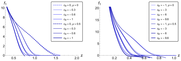
A                                                                 B

Figure 12: The coupling function $f_{1}(z)$ for different $c_{B}\geq-\,1$, $\mu=0$ (light blue) and $\mu=0.5$ (dark blue), $z_{h_{min}}\geq 0.73$ (A); for different $c_{B}\leq-\,1$, $\mu=0.5$, $z_{h_{min}}\geq 0.39$ (B); $\nu=4.5$, $z_{h}=1.5$, $R_{gg}=1.16$, $p=0.273$, $q_{3}=5$, $q_{1}=1$; $[z]^{-1}=$ GeV.

Fig.12 shows the coupling function $f_{1}$ in terms of holographic coordinate $z$. It gets positive value for zero chemical potential (Fig.12.A, light blue), so the NEC is fulfilled in our model. For perceptible chemical potential value $\mu=0.5$ (Fig.12.A, dark blue) the coupling function $f_{1}$ can be not positive for $z<z_{h}$ in magnetic field strong enough. But the second horizon shift under the first (fixed) one must be taken in account again. For $z<z_{h_{2}}$ the coupling function $f_{1}$ stays positive similar to the coupling function $f_{3}$, thus NEC is respected (Fig.12.B, the second horizon $z_{h_{min}}=z_{h_{2}}=0.39$). For $f_{1}$ it can be proven algebraically, like it was done for it in [1] and for $f_{3}$ in previous section, that it doesn’t break the NEC either. According to the boundary condition $g(z_{h})=0$ expression for $f_{1}$ can be simplified as

$$f_{1}(z_{h})=-\,2\left(\cfrac{z_{h}}{L}\right)^{1-\frac{4}{\nu}}\cfrac{\nu-1}{L\,q_{1}^{2}\nu}\ e^{c_{B}z_{h}^{2}}\ \mathfrak{b}(z_{h})\,g^{\prime}(z_{h}).$$ (3.23)

At the first horizon $z_{h}=z_{h_{min}}$ the blackening function is decreasing, so $g^{\prime}(z_{h})<0$ and temperature $T(z_{h})=|g^{\prime}(z_{h})/4\pi|$ is positive. As $f_{1}$ has sense for $\nu>1$ only, all the multipliers in (3.23) are positive, so their product is positive, therefore $f_{1}(z_{h})>0$ for any $z_{h}$ from the interval $0<z_{h}<z_{h_{min}}$, where $z_{h_{min}}$ is the actual horizon, i.e. $T(z_{h_{min}})=0$.

For the completeness of the results presented the second coupling function $f_{1}(\phi)$ is also plotted (Fig.13). It turns out to be insensitive to the magnetic field for small $\phi$ values and almost insensitive to the fixed horizon value even for large $\phi$ (Fig.13.A). Besides, the magnetic field shifts $f_{1}$ up to larger values, while the chemical potential, on the contrary, downs to smaller values (Fig.13.B).

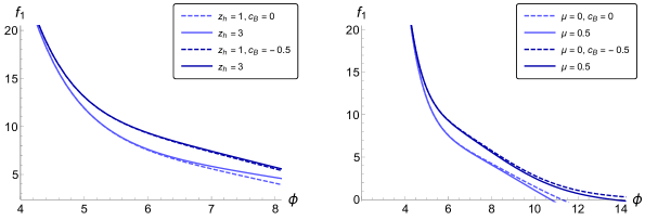
A                                                                 B

Figure 13: The coupling function $f_{1}(\phi)$ for different $z_{h}$ and $c_{B}$, $\mu=0.5$ (A), for different $\mu$ and $c_{B}$ and $z_{h}=1$; $\nu=4.5$, $R_{gg}=1.16$, $p=0.273$, $q_{3}=5$, $z_{0}=0.001$.

3.2.5 Scalar potential

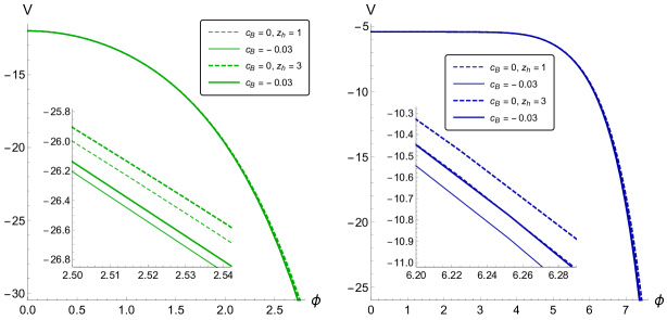
A                                                                 B

Figure 14: The scalar potential $V(\phi)$ for different $c_{B}$ and $z_{h}$, $\nu=1$ (A) and $\nu=4.5$ (B); $R_{gg}=1.16$, $p=0.273$, $q_{3}=5$, $\mu=0.5$, $z_{0}=0.001$; $[V]=$ GeV².

The equation of motion for the scalar potential $V$ as a function of holographic coordinate $z$ can be obtained from the equation (A.18):

$$\begin{split}V(z)=-\,\cfrac{3}{2L^{2}\nu^{2}\mathfrak{b}}&\left[\Biggl{\{}\cfrac{\mathfrak{b}^{\prime\prime}}{\mathfrak{b}}\ \nu^{2}z^{2}+\cfrac{(\mathfrak{b}^{\prime})^{2}}{2\mathfrak{b}^{2}}\ \nu^{2}z^{2}-\cfrac{\mathfrak{b}^{\prime}}{\mathfrak{b}}\ \bigl{(}3(1+\nu)-2c_{B}\nu z^{2}\bigr{)}\nu z\right.+\\ &\ \ +\cfrac{2}{3}\ \bigl{(}2(1+\nu)(1+2\nu)-(3+2\nu)c_{B}\nu z^{2}+c_{B}^{2}\nu^{2}z^{4}\bigr{)}\Biggr{\}}\,g\ +\\ &\ \ +\left.\left\{\cfrac{3\mathfrak{b}^{\prime}}{2\mathfrak{b}}\,\nu z-\cfrac{4+5\nu}{3}+c_{B}\nu z^{2}\right\}\nu zg^{\prime}+\cfrac{\nu^{2}z^{2}}{3}\,g^{\prime\prime}\right].\end{split}$$ (3.24)

The exact formula obtained by substituting the blackening function, its first and second derivatives and the new corrected warp factor is presented in Appendix B.

The scalar potential $V$ as a function of dilaton field $\phi$ is described by equations (3.20) and (3.24) and is depicted in Fig.14. Within the interval $0\leq z\leq z_{h}$, that we are interested in, $V(\phi)$ is stable and has no crucial dependence either on the horizon nor on the magnetic field. More focus in the scale allows to see that the magnetic field increases the absolute value of the scalar potential, while $z_{h}$ growth decreases it. Primary anisotropy (Fig.14.B for $\nu=4.5$) shifts the scalar potential to larger absolute values (Fig.14.A for $\nu=1$), causes a constant region to appear at small $\phi$ and then makes $V(\phi)$ to decrease faster.

3.3 Thermodynamics for ${\cal A}(z)=-\,cz^{2}/4\,-(p-c_{B}q_{3})z^{4}$

3.3.1 Temperature and entropy

Using the metric (2.6) and the warp factor $\mathfrak{b}(z)=e^{-\,cz^{2}/2\,-\,2(p-c_{B}\,q_{3})z^{4}}$ (3.16) one can obtain the temperature and entropy from equations (3.12) and (3.13) respectively:

$$\begin{split}T&=\cfrac{|g^{\prime}|}{4\pi}\,\Biggl{|}_{z=z_{h}}=\left|-\,\cfrac{e^{(2R_{gg}-c_{B})\frac{z_{h}^{2}}{2}+3(p-c_{B}\,q_{3})z_{h}^{4}}\,z_{h}^{1+\frac{2}{\nu}}}{4\pi\,\tilde{I}_{1}(z_{h})}\right.\times\\ &\left.\times\left[1-\cfrac{\mu^{2}\bigl{(}2R_{gg}+c_{B}(q_{3}-1)\bigr{)}\left(e^{(2R_{gg}+c_{B}(q_{3}-1))\frac{z_{h}^{2}}{2}}\tilde{I}_{1}(z_{h})-\tilde{I}_{2}(z_{h})\right)}{L^{2}\left(1-e^{(2R_{gg}+c_{B}(q_{3}-1))\frac{z_{h}^{2}}{2}}\right)^{2}}\right]\right|,\\ s=\ &\cfrac{1}{4}\left(\cfrac{L}{z_{h}}\right)^{1+\frac{2}{\nu}}e^{-(2R_{gg}-c_{B})\frac{z_{h}^{2}}{2}-3(p-c_{B}\,q_{3})z_{h}^{4}}.\end{split}$$ (3.25)

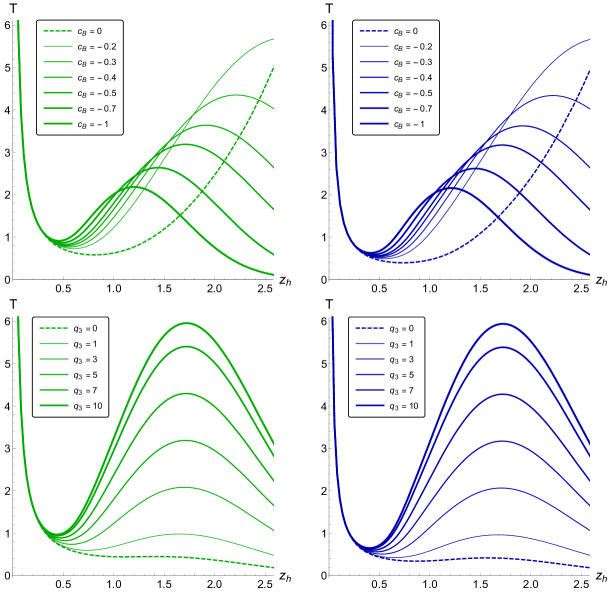
A                                                                 B

Figure 15: Temperature $T(z_{h})$ for different $c_{B}$, $q_{3}=5$ (1-st line) and for different $q_{3}$, $c_{B}=-\,0.5$ (2-nd line); $\nu=1$ (A) and $\nu=4.5$ (B); $R_{gg}=1.16$, $p=0.273$, $\mu=0$; $[T]=[z_{h}]^{-1}=$ GeV.

A                                                                 B

Figure 16: Temperature $T(z_{h})$ for different $c_{B}$, $q_{3}=5$ (1-st line) and for different $q_{3}$, $c_{B}=-\,0.5$ (2-nd line); $\nu=1$ (A) and with $\nu=4.5$ (B); $R_{gg}=1.16$, $p=0.273$, $\mu=0.3$; $[T]=[z_{h}]^{-1}=$ GeV.

The behavior of the temperature $T$ as a function of the horizon radius $z_{h}$ for different values of the magnetic coefficient $c_{B}$ (1-st line) and the magnetic “charge” $q_{3}$ (2-nd line) in backgrounds with different primary anisotropy $\nu=1$ (A) and $\nu=4.5$ (B) and zero chemical potential $\mu=0$ is shown in Fig.15. The system temperature is obviously sensible to the magnetic field parameters in such a way that the temperature minimum grows with the magnetic coefficient $c_{B}$ absolute value (Fig.15, 1-st line) and the magnetic “charge” $q_{3}$ (Fig.15, 2-nd line). Naively, it means that the Hawking-Page phase transition temperature $T_{HP}$ value increases with the magnetic field in all the cases considered. Note that to investigate the magnetic field effect on the phase transition temperature below, we consider the magnetic coefficient $c_{B}$, although the magnetic “charge” $q_{3}$ acts on the transition temperature in a similar way. As to the primary anisotropy, it makes the temperature local minimum to decrease both for various $c_{B}$ and $q_{3}$. Therefore, one can expect the Hawking-Page phase transition temperature $T_{HP}$ to increase during the isotropisation process. But to check this point and the BB phase transition explicitly, we need to calculate the free energy of the system.

A                                                                 B

Figure 17: Free energy $F(T)$ for different $c_{B}$, $q_{3}=5$ (1-st line) and for different $q_{3}$, $c_{B}=-\,0.5$ (2-nd line); $\nu=1$ (A) and $\nu=4.5$ (B); $R_{gg}=1.16$, $p=0.273$, $\mu=0$; $[F]=[T]=$ GeV.

Now, we consider the non-zero chemical potential as we need to include matter to investigate the realistic QGP with high baryonic density. In Fig.16 the system temperature $T$ in terms of the horizon $z_{h}$ at the chemical potential $\mu=0.3$ for different values of $c_{B}$ (1-st line) and $q_{3}$ (2-nd line) is plotted. The temperature is still very sensible to both magnetic field parameters, and the Hawking-Page phase transition temperature $T_{HP}$ increases. Primary anisotropy makes the temperature local minimum to decrease again and therefore the Hawking-Page phase transition $T_{HP}$ requires less energy. To investigate the process precisely we need to plot a free energy for different chemical potential values.

A                                                                 B

Figure 18: Free energy $F(T)$ for different $c_{B}$, $q_{3}=5$ (1-st line) and $q_{3}$, $c_{B}=-\,0.5$ (2-nd line); $\nu=1$ (A) and $\nu=4.5$ (B); $R_{gg}=1.16$, $p=0.273$, $\mu=0.3$, in units $[F]=[T]=$ GeV.

3.3.2 Free energy and magnetic catalysis

To investigate the first order phase transition we start from the free energy $F$ as a function of temperature $T$ consideration for different values of the magnetic field parameters $c_{B}$ and $q_{3}$ at zero chemical potential. Regardless of the primary background anisotropy ($\nu=1$ in Fig.17.A and $\nu=4.5$ in Fig.17.B) the free energy is a multivalued function of temperature and at $\mu=0$ has two branches. One of them is positive but asymptotically decreasing to zero, the other goes down into the region of negative values sharply, almost vertically. The negative part of this branch describes the large stable black hole, positive free energy values correspond to the small unstable black hole and at $F=0$ thermal gas is formed. Temperature of the phase transition from a small black hole to thermal gas known as Hawking-Page phase transition is so called Hawking-Page temperature, $F(T_{HP})=0$. According to the holographic dictionary this process corresponds to the first order phase transition in the dual 4-dim gauge theory. To reveal the magnetic field effect on the free energy behavior and, consequently, on the phase transition temperature $T_{HP}$, we increase the absolute values of the magnetic parameters $c_{B}$ (Fig.17, 1-st line) and $q_{3}$ (Fig.17, 2-nd line). In both cases $T_{HP}$ grows, thus the magnetic catalysis phenomenon takes place for any primary anisotropy, but in the background with higher primary anisotropy phase transition requires lower temperature, like it was in previous works [1, 49, 37, 38, 39, 40].

A                                         B                                         C

Figure 19: $T_{HP}$ as a function of $c_{B}$, $\mu=0$ (A), $T_{BB}$ as a function of $c_{B}$, $\mu=0.3$ (B) and their comparison (C); $\nu=1$ (green lines) and $\nu=4.5$ (blue lines); $R_{gg}=1.16$, $p=0.273$, $q_{3}=5$; $[T]=[c_{B}]^{1/2}=$ GeV.

At a non-zero chemical potential there appears the free energy third (almost horizontal) branch, and a closed structure called a “swallow-tail” appears (Fig.18, $\mu=0.3$). Its self-intersection point describes the first order phase transition, and its temperature is marked as BB temperature $T_{BB}$. All other tendencies preserve: magnetic field parameters $c_{B}$ and $q_{3}$ cause the phase transition growth while the primary anisotropy $\nu$ lowers it. This allows us to expect the MC-effect to be general on the first order phase diagram. All these results are summarized in Fig.19, where the phase transition temperature dependence on the magnetic coefficient $c_{B}$ for $\mu=0$ (A) and $\mu=0.3$ (B) in the background with different primary anisotropy is depicted; the results for various chemical potentials in primary isotropic case are confronted in Fig.19.C.

A                                                                    B

Figure 20: Temperature $T(z_{h})$ for different $\mu$ (A) and free energy $F(T)$ for different $\mu$ (B); $\nu=1$ (1-st line) and $\nu=4.5$ (2-nd line); $R_{gg}=1.16$, $p=0.273$, $q_{3}=5$ and $c_{B}=-\,0.5$, in units $[T]=[z_{h}]^{-1}=$ GeV.

To obtain the full picture of the first order phase transition the free energy and consequently the temperature dependence on the chemical potential should be considered. At $\mu=0$ the temperature has minimum $T_{min}=T(z_{min})$ (Fig.20.A). Black hole solutions with $z_{h}>z_{min}$ (small black holes) are unstable, and the essence of the phase transition lies in the collapse of such a black hole into a stable black hole with the same temperature, but $z_{h}<z_{min}$ (large black holes). There is no black hole solution for $T<T_{min}$, therefore Hawking-Page phase transition occurs at $T_{HP}\geq T_{min}$. At the very point $T_{min}$ a large stable black hole transforms into the thermal gas. This point is clearly seen on the free energy plot as $F(T_{min})=0$ (Fig.20.B).

For $\mu>0$ the function $T(z_{h})$ also has a local maximum $T_{max}=T(z_{max})$, where $z_{max}>z_{min}$ (Fig.20.A), and this leads to the “swallow-tail” appearance in the free energy plot again (Fig.20.B). Temperature of the phase transition, i.e. the collapse from a small unstable black hole to a large stable black hole, can be determined as the temperature of the self-intersection point in the “swallow-tail” base of the $F(T)$-curve. As the chemical potential increases both $T(z_{min})$ and $T(z_{max})$ decrease so that the difference between them reduces and eventually disappears at some critical value of the chemical potential. For example, in the magnetic field with $c_{B}=-\,0.5$ for $\nu=1$ and $\nu=4.5$ it happens at $\mu_{CEP_{HQ}}\approx 0.94$ and $\mu_{CEP_{HQ}}\approx 0.81$ correspondingly (Fig.20.A). This process is reflected by the “swallow-tail” decrease on the free energy plot (Fig.20.B). For $\mu>\mu_{CEP_{HQ}}$ the black hole temperature becomes a monotonic function of the horizon and its free energy becomes smooth. Note that additional details on this subject can be found in papers on previous considerations [45, 46, 1].

3.3.3 Phase diagrams

A                                                                 B

C                                                                 D

Figure 21: The phase diagrams in the $(\mu,T)$-plane for heavy quarks with different $c_{B}$ for $\nu=1$ (A) and $\nu=4.5$ (B), the comparison between $\nu=1$ and $\nu=4.5$ (C); $R_{gg}=1.16$, $p=0.273$, $q_{3}=5$, in units $[T]=[\mu]=$ GeV; the phase diagrams in the $(\mu,T)$-plane for light quarks (D) from [49]. In all plots we considered $\nu=1$ (green lines) and $\nu=4.5$ (blue lines) for different $c_{B}$.

Phase diagram, i.e. the diagram of the confinement/deconfinement phase transition displays the dependence of the phase transition temperature on the chemical potential. This phase diagram consists of two different phase transition lines, i.e. first order phase transition line and phase transition line for temporal Wilson loops on the $(\mu$,$T)$-plane. In this research we considered the first order phase transition only. In the “heavy quarks” version of our holographic model the phase transition line stretches over the interval $\mu\in[0,\mu_{max}]$, and the temperature in this interval drops (Fig.21). The rightmost point of the curve with coordinates $\bigl{(}\mu_{max},T(\mu_{max})\bigr{)}$ is called a critical end point ($CEP_{HQ}$ for heavy quarks) and marks the free (not attached to the axis) end of the phase transition line (dots on the right end of the $T(\mu)$-curves).

First of all, we really see the MC effect in the background with any amount of anisotropy. For $\nu=1$ CEP chemical potential $\mu_{CEP_{HQ}}$ grows by increasing $|c_{B}|$ for the region $0<\,|c_{B}|<\,0.5$, after that $\mu_{CEP_{HQ}}$ decreases by increasing $|c_{B}|$ and gets zero at $|c_{B}|=6$ when the phase transition line completely disappears (Fig.21.A). For $\nu=4.5$ $\mu_{CEP_{HQ}}$ decreases by increasing $|c_{B}|$, and the phase transition line shortens until complete disappearence at $|c_{B}|\sim\,10$, (Fig.21.B). We presented critical end points for different $c_{B}$ with $\nu=1$ and $\nu=4.5$ in Table 1.

$\nu=1$	$(\mu_{CEP_{HQ}},T_{CEP_{HQ}})$	$\nu=4.5$	$(\mu_{CEP_{HQ}},T_{CEP_{HQ}})$
$c_{B}=0$	(0.74, 0.52)	$c_{B}=0$	(0.91, 0.27)
$c_{B}=-\,0.1$	(0.85, 0.61)	$c_{B}=-\,0.5$	(0.81, 0.43)
$c_{B}=-\,0.5$	(0.94, 0.76)	$c_{B}=-\,1$	(0.74, 0.50)
$c_{B}=-\,1$	(0.93, 0.85)	$c_{B}=-\,2$	(0.62, 0.59)
$c_{B}=-\,3$	(0.67, 1.00)	$c_{B}=-\,4$	(0.50, 0.70)
$c_{B}=-\,5$	(0.33, 1.04)	$c_{B}=-\,6$	(0.36, 0.75)
$c_{B}=-\,5.5$	(0.18, 1.04)	$c_{B}=-\,8$	(0.23, 0.79)
—	—	$c_{B}=-\,9.6$	(0.06, 0.81)

Table 1: The critical end points for different $c_{B}$ with $\nu=1$ and $\nu=4.5$

In both cases the $T_{HP/BB}$ rise slows down with increasing magnetic field, before the complete disappearance of phase transition lines it stops and even turns back. We observed that for the small region the IMC appears at near-limit $c_{B}$ values, namely $|c_{B}|>\,5$ for $\nu=1$ and $|c_{B}|>\,8$ for $\nu=4.5$ (light green and blue curves, respectively). But it is obvious that in the primary isotropic background the phase transition degenerates at a magnetic field weaker than in the primary anisotropic one. Besides for $\nu=4.5$ phase transition temperature is lower and drops faster as $\mu$ increases (Fig.21.C). We can compare heavy quarks phase diagrams (Fig.21.A,B,C) that describe MC and light quarks phase diagram (Fig.21.D) that presents IMC phenomenon [49].

4 Conclusion and Discussion

In this research we studied the influence of the magnetic field on the first order phase transition temperature. For this purpose we used the “bottom-up” approach and chose 5-dim Einstein-dilaton-Maxwell holographic model with three Maxwell fields. In previous paper [1] only the IMC phenomenon was obtained. In this research we look for a warp factor, that serves for a deformation of metric, providing the MC phenomenon for the heavy quark model [1]. As our holographic model is phenomenological, there is no systematic way to construct it. We have to use the trial and error method to get results compatible with existing experiments and others theoretical methods.

Let us summarize our main results.

• A new 5-dim exact analytical solution for anisotropic holographic model of QGP is presented. One of its important features is inclusion of two types of anisotropy, caused by the spatial anisotropy, called primary, and the external magnetic field. Their influences on the background physical properties such as background phase transition are investigated.

• Choosing the warp factor that deforms the metric is a key point of the current research. The warp factor $\mathfrak{b}(z)=e^{2{\cal A}(z)}=e^{-\,cz^{2}/2\,-\,2pz^{4}}$ leads to IMC in the sense of decreasing of the critical temperature with increasing the magnetic field $B$.

• The MC effect is achieved for the warp factor $\mathfrak{b}(z)=e^{-\,cz^{2}/2\,-\,2(p-c_{B}\,q_{3})z^{4}}$ for $c_{B}$ not to be large (see discussion of the Figure 21). This takes place for zero chemical potential, i.e. for Hawking-Page-like (HP) phase transition, and for non-zero chemical potential, i.e. black hole-black hole first order. In both cases we get MC in the dual 4-dim gauge theory.

• The effect of primary anisotropy on black hole-black hole (BB) and Hawking-Page-like (HP) phase transition is investigated. It is found that anisotropy decreases both $T_{HP}$ and $T_{BB}$ for all values of magnetic field.

• The phase diagram, i.e. the dependence of the phase transition temperature on chemical potential, is built for different magnetic field magnitudes and different primary anisotropy values within the model constructed.

• Complete disappearance of the phase transition lines for the primary isotropic background, $\nu=1$, occurs at weaker magnetic field ($|c_{B}|\sim\,6$) in comparison to the anisotropic one, $\nu=4.5$ ($|c_{B}|\sim\,10$).

• Even for the near-limit chemical potential values the NEC to be preserved, as the consideration has sense and can be performed within the physical interval between the boundary and the second horizon in this model.

• It is expected that for the presented model different quantities such as baryon density, entanglement entropy, electrical conductivity should have jump in the vicinity of the first order phase transition. This jump should strongly depend on the model parameters (anisotropy, magnetic field, chemical potential etc.) similar to previously considered models [97, 49, 83].

• In [1, 45, 50, 112] the temporal and spatial Wilson loops were considered on the background for heavy quarks with two types of anisotropy with the warp factor $\mathfrak{b}(z)=e^{-\,cz^{2}/2}$. It would be interesting to study phase transition on this background with the new corrected warp factor. Also one can investigate energy loss and jet quenching on this background similar to [113]. This will allow to obtain full confinement/deconfinement phase transition structure, that is determined by the Wilson loop and first order phase transition interplay.

In this paper we do not make calculations of the chiral condensate $\langle\bar{\psi}\psi\rangle$. We would like to emphasize that to calculate $\langle\bar{\psi}\psi\rangle$ one has to consider a new action, i.e. chiral action including a few new fields $\chi$, and solve corresponding equations of motion. We do not perform these calculations in the present paper, this will be the subject of the future investigations. Similar calculations have been performed in [114, 115, 54] in different models. The chiral condensate $\langle\bar{\psi}\psi\rangle$ has been calculated for light quark models in [114, 115] for zero magnetic field. The chiral condensate $\langle\bar{\psi}\psi\rangle$ has been calculated in [54] for non zero $B$ for the heavy quark holographic model with IMC in the sense of decreasing of the critical temperature with increasing $B$ (i.e. without extra term $z^{4}$ in the warp factor). It has been found that $\langle\bar{\psi}\psi\rangle$ increasing with increasing $B$ that could be called MC in the sense of the condensate value.

5 Acknowledgements

The work of I.A. and A.H. was performed at the Steklov International Mathematical Center and supported by the Ministry of Science and Higher Education of the Russian Federation (Agreement No.075-15-2022-265). The work of K.R. was performed within the scientific project No. FSSF-2023-0003. K.R. and P.S. thank the “BASIS” Science Foundation (grants No. 22-1-3-18-1 and No. 21-1-5-127-1, No. 23-1-4-43-1).

Appendix A Equations of motion

Varying Lagrangian (2.1) over metric (2.6) we get 5 Einstein equations of motions:

$$\begin{split}{\bf 00}:\quad&-\left(\cfrac{L}{z}\right)^{3+\frac{2}{\nu}}e^{c_{B}z^{2}/2}\,\mathfrak{b}^{5/2}g\left[\cfrac{g^{\prime}}{2}\left(\cfrac{3\mathfrak{b}^{\prime}}{2\mathfrak{b}}-\cfrac{2+\nu\,(1-c_{B}z^{2})}{\nu z}\right)\right.\\ &+g\left(\cfrac{3\mathfrak{b}^{\prime\prime}}{2\mathfrak{b}}-\cfrac{3\mathfrak{b}^{\prime 2}}{4\mathfrak{b}^{2}}-\cfrac{3\mathfrak{b}^{\prime}}{2\mathfrak{b}}\ \cfrac{2-\nu c_{B}z^{2}}{\nu z}+\cfrac{3+2\nu+\nu^{2}}{\nu^{2}z^{2}}-\cfrac{c_{B}\big{(}3-\nu\,(1+c_{B}z^{2})\big{)}}{\nu}\right)\\ &+\left.\left(\cfrac{z}{L}\right)^{2}\cfrac{f_{0}A_{t}^{\prime 2}}{4\mathfrak{b}}+\left(\cfrac{L}{z}\right)^{2-\frac{4}{\nu}}\cfrac{e^{-c_{B}z^{2}}f_{1}q_{1}^{2}}{4\mathfrak{b}}+\left(\cfrac{z}{L}\right)^{\frac{2}{\nu}}\cfrac{f_{3}q_{3}^{2}}{4\mathfrak{b}}+\cfrac{g}{4}\,\phi^{\prime 2}+\left(\cfrac{L}{z}\right)^{2}\cfrac{\mathfrak{b}V}{2}\right]=0,\end{split}$$ (A.1)

$$\begin{split}{\bf 11}:\quad&-\left(\cfrac{L}{z}\right)^{3+\frac{2}{\nu}}e^{c_{B}z^{2}/2}\,\mathfrak{b}^{5/2}\left[\cfrac{g^{\prime\prime}}{2}+g^{\prime}\left(\cfrac{3\mathfrak{b}^{\prime}}{2\mathfrak{b}}-\cfrac{2+\nu\,(1-c_{B}z^{2})}{\nu z}\right)\right.\\ &+g\left(\cfrac{3\mathfrak{b}^{\prime\prime}}{2\mathfrak{b}}-\cfrac{3\mathfrak{b}^{\prime 2}}{4\mathfrak{b}^{2}}-\cfrac{3\mathfrak{b}^{\prime}}{2\mathfrak{b}}\ \cfrac{2-\nu c_{B}z^{2}}{\nu z}+\cfrac{3+2\nu+\nu^{2}}{\nu^{2}z^{2}}-\cfrac{c_{B}\big{(}3-\nu\,(1+c_{B}z^{2})\big{)}}{\nu}\right)\\ &-\left.\left(\cfrac{z}{L}\right)^{2}\cfrac{f_{0}A_{t}^{\prime 2}}{4\mathfrak{b}}+\left(\cfrac{L}{z}\right)^{2-\frac{4}{\nu}}\cfrac{e^{-c_{B}z^{2}}f_{1}q_{1}^{2}}{4\mathfrak{b}}-\left(\cfrac{z}{L}\right)^{\frac{2}{\nu}}\cfrac{f_{3}q_{3}^{2}}{4\mathfrak{b}}+\cfrac{g}{4}\,\phi^{\prime 2}+\left(\cfrac{L}{z}\right)^{2}\cfrac{\mathfrak{b}V}{2}\right]=0,\end{split}$$ (A.2)

$$\begin{split}{\bf 22}:\quad&-\left(\cfrac{L}{z}\right)^{1+\frac{4}{\nu}}e^{c_{B}z^{2}/2}\,\mathfrak{b}^{5/2}\left[\cfrac{g^{\prime\prime}}{2}+g^{\prime}\left(\cfrac{3\mathfrak{b}^{\prime}}{2\mathfrak{b}}-\cfrac{1+\nu\,(2-c_{B}z^{2})}{\nu z}\right)\right.\\ &+g\left(\cfrac{3\mathfrak{b}^{\prime\prime}}{2\mathfrak{b}}-\cfrac{3\mathfrak{b}^{\prime 2}}{4\mathfrak{b}^{2}}-\cfrac{3\mathfrak{b}^{\prime}}{2\mathfrak{b}}\ \cfrac{1+\nu\,(1-c_{B}z^{2})}{\nu z}+\cfrac{1+2\nu+3\nu^{2}}{\nu^{2}z^{2}}-\cfrac{c_{B}(2-\nu c_{B}z^{2})}{\nu}\right)\\ &-\left.\left(\cfrac{z}{L}\right)^{2}\cfrac{f_{0}A_{t}^{\prime 2}}{4\mathfrak{b}}-\left(\cfrac{L}{z}\right)^{2-\frac{4}{\nu}}\cfrac{e^{-c_{B}z^{2}}f_{1}q_{1}^{2}}{4\mathfrak{b}}-\left(\cfrac{z}{L}\right)^{\frac{2}{\nu}}\cfrac{f_{3}q_{3}^{2}}{4\mathfrak{b}}+\cfrac{g}{4}\,\phi^{\prime 2}+\left(\cfrac{L}{z}\right)^{2}\cfrac{\mathfrak{b}V}{2}\right]=0,\end{split}$$ (A.3)

$$\begin{split}{\bf 33}:\quad&-\left(\cfrac{L}{z}\right)^{1+\frac{4}{\nu}}e^{3c_{B}z^{2}/2}\,\mathfrak{b}^{5/2}\left[\cfrac{g^{\prime\prime}}{2}+g^{\prime}\left(\cfrac{3\mathfrak{b}^{\prime}}{2\mathfrak{b}}-\cfrac{1+2\nu}{\nu z}\right)\right.\\ &+g\left(\cfrac{3\mathfrak{b}^{\prime\prime}}{2\mathfrak{b}}-\cfrac{3\mathfrak{b}^{\prime 2}}{4\mathfrak{b}^{2}}-\cfrac{3\mathfrak{b}^{\prime}}{2\mathfrak{b}}\ \cfrac{1+\nu}{\nu z}+\cfrac{1+2\nu+3\nu^{2}}{\nu^{2}z^{2}}\right)\end{split}$$ (A.4)

$$-\left.\left(\cfrac{z}{L}\right)^{2}\cfrac{f_{0}A_{t}^{\prime 2}}{4\mathfrak{b}}-\left(\cfrac{L}{z}\right)^{2-\frac{4}{\nu}}\cfrac{e^{-c_{B}z^{2}}f_{1}q_{1}^{2}}{4\mathfrak{b}}+\left(\cfrac{z}{L}\right)^{\frac{2}{\nu}}\cfrac{f_{3}q_{3}^{2}}{4\mathfrak{b}}+\cfrac{g}{4}\,\phi^{\prime 2}+\left(\cfrac{L}{z}\right)^{2}\cfrac{\mathfrak{b}V}{2}\right]=0,$$

$$\begin{split}{\bf 44}:\quad&-\left(\cfrac{L}{z}\right)^{3+\frac{2}{\nu}}e^{c_{B}z^{2}/2}\,\cfrac{\mathfrak{b}^{5/2}}{g}\left[\cfrac{g^{\prime}}{2}\left(\cfrac{3\mathfrak{b}^{\prime}}{2\mathfrak{b}}-\cfrac{2+\nu\,(1-c_{B}z^{2})}{\nu z}\right)\right.\\ &+g\left(\cfrac{3\mathfrak{b}^{\prime 2}}{2\mathfrak{b}^{2}}-\cfrac{3\mathfrak{b}^{\prime}}{2\mathfrak{b}}\ \cfrac{2+\nu\,(2-c_{B}z^{2})}{\nu z}+\cfrac{1+4\nu+\nu^{2}}{\nu^{2}z^{2}}-\cfrac{1+2\nu}{\nu}\ c_{B}\right)\\ &+\left.\left(\cfrac{z}{L}\right)^{2}\cfrac{f_{0}A_{t}^{\prime 2}}{4\mathfrak{b}}+\left(\cfrac{L}{z}\right)^{2-\frac{4}{\nu}}\cfrac{e^{-c_{B}z^{2}}f_{1}q_{1}^{2}}{4\mathfrak{b}}+\left(\cfrac{z}{L}\right)^{\frac{2}{\nu}}\cfrac{f_{3}q_{3}^{2}}{4\mathfrak{b}}-\cfrac{g}{4}\,\phi^{\prime 2}+\left(\cfrac{L}{z}\right)^{2}\cfrac{\mathfrak{b}V}{2}\right]=0.\end{split}$$ (A.5)

We rewrite these 5 Einstein equations (remove factors in front of (A.1-A.5)) as:

$$\begin{split}{\bf[00]}:\quad&\cfrac{g^{\prime}}{2}\left(\cfrac{3\mathfrak{b}^{\prime}}{2\mathfrak{b}}-\cfrac{2+\nu\,(1-c_{B}z^{2})}{\nu z}\right)\\ &+g\left(\cfrac{3\mathfrak{b}^{\prime\prime}}{2\mathfrak{b}}-\cfrac{3\mathfrak{b}^{\prime 2}}{4\mathfrak{b}^{2}}-\cfrac{3\mathfrak{b}^{\prime}}{2\mathfrak{b}}\ \cfrac{2-\nu c_{B}z^{2}}{\nu z}+\cfrac{3+2\nu+\nu^{2}}{\nu^{2}z^{2}}-\cfrac{c_{B}\big{(}3-\nu\,(1+c_{B}z^{2})\big{)}}{\nu}\right)\\ &+\left(\cfrac{z}{L}\right)^{2}\cfrac{f_{0}A_{t}^{\prime 2}}{4\mathfrak{b}}+\left(\cfrac{L}{z}\right)^{2-\frac{4}{\nu}}\cfrac{e^{-c_{B}z^{2}}f_{1}q_{1}^{2}}{4\mathfrak{b}}+\left(\cfrac{z}{L}\right)^{\frac{2}{\nu}}\cfrac{f_{3}q_{3}^{2}}{4\mathfrak{b}}+\cfrac{g}{4}\,\phi^{\prime 2}+\left(\cfrac{L}{z}\right)^{2}\cfrac{\mathfrak{b}V}{2}=0,\end{split}$$ (A.6)

$$\begin{split}{\bf[11]}:\quad&\cfrac{g^{\prime\prime}}{2}+g^{\prime}\left(\cfrac{3\mathfrak{b}^{\prime}}{2\mathfrak{b}}-\cfrac{2+\nu\,(1-c_{B}z^{2})}{\nu z}\right)\\ &+g\left(\cfrac{3\mathfrak{b}^{\prime\prime}}{2\mathfrak{b}}-\cfrac{3\mathfrak{b}^{\prime 2}}{4\mathfrak{b}^{2}}-\cfrac{3\mathfrak{b}^{\prime}}{2\mathfrak{b}}\ \cfrac{2-\nu c_{B}z^{2}}{\nu z}+\cfrac{3+2\nu+\nu^{2}}{\nu^{2}z^{2}}-\cfrac{c_{B}\big{(}3-\nu\,(1+c_{B}z^{2})\big{)}}{\nu}\right)\\ &-\left(\cfrac{z}{L}\right)^{2}\cfrac{f_{0}A_{t}^{\prime 2}}{4\mathfrak{b}}+\left(\cfrac{L}{z}\right)^{2-\frac{4}{\nu}}\cfrac{e^{-c_{B}z^{2}}f_{1}q_{1}^{2}}{4\mathfrak{b}}-\left(\cfrac{z}{L}\right)^{\frac{2}{\nu}}\cfrac{f_{3}q_{3}^{2}}{4\mathfrak{b}}+\cfrac{g}{4}\,\phi^{\prime 2}+\left(\cfrac{L}{z}\right)^{2}\cfrac{\mathfrak{b}V}{2}=0,\end{split}$$ (A.7)

$$\begin{split}{\bf[22]}:\quad&\cfrac{g^{\prime\prime}}{2}+g^{\prime}\left(\cfrac{3\mathfrak{b}^{\prime}}{2\mathfrak{b}}-\cfrac{1+\nu\,(2-c_{B}z^{2})}{\nu z}\right)\\ &+g\left(\cfrac{3\mathfrak{b}^{\prime\prime}}{2\mathfrak{b}}-\cfrac{3\mathfrak{b}^{\prime 2}}{4\mathfrak{b}^{2}}-\cfrac{3\mathfrak{b}^{\prime}}{2\mathfrak{b}}\ \cfrac{1+\nu\,(1-c_{B}z^{2})}{\nu z}+\cfrac{1+2\nu+3\nu^{2}}{\nu^{2}z^{2}}-\cfrac{c_{B}(2-\nu c_{B}z^{2})}{\nu}\right)\end{split}$$ (A.8)

$$-\left(\cfrac{z}{L}\right)^{2}\cfrac{f_{0}A_{t}^{\prime 2}}{4\mathfrak{b}}-\left(\cfrac{L}{z}\right)^{2-\frac{4}{\nu}}\cfrac{e^{-c_{B}z^{2}}f_{1}q_{1}^{2}}{4\mathfrak{b}}-\left(\cfrac{z}{L}\right)^{\frac{2}{\nu}}\cfrac{f_{3}q_{3}^{2}}{4\mathfrak{b}}+\cfrac{g}{4}\,\phi^{\prime 2}+\left(\cfrac{L}{z}\right)^{2}\cfrac{\mathfrak{b}V}{2}=0,$$

$$\begin{split}{\bf[33]}:\quad&\cfrac{g^{\prime\prime}}{2}+g^{\prime}\left(\cfrac{3\mathfrak{b}^{\prime}}{2\mathfrak{b}}-\cfrac{1+2\nu}{\nu z}\right)\\ &+g\left(\cfrac{3\mathfrak{b}^{\prime\prime}}{2\mathfrak{b}}-\cfrac{3\mathfrak{b}^{\prime 2}}{4\mathfrak{b}^{2}}-\cfrac{3\mathfrak{b}^{\prime}}{2\mathfrak{b}}\ \cfrac{1+\nu}{\nu z}+\cfrac{1+2\nu+3\nu^{2}}{\nu^{2}z^{2}}\right)\\ &-\left(\cfrac{z}{L}\right)^{2}\cfrac{f_{0}A_{t}^{\prime 2}}{4\mathfrak{b}}-\left(\cfrac{L}{z}\right)^{2-\frac{4}{\nu}}\cfrac{e^{-c_{B}z^{2}}f_{1}q_{1}^{2}}{4\mathfrak{b}}+\left(\cfrac{z}{L}\right)^{\frac{2}{\nu}}\cfrac{f_{3}q_{3}^{2}}{4\mathfrak{b}}+\cfrac{g}{4}\,\phi^{\prime 2}+\left(\cfrac{L}{z}\right)^{2}\cfrac{\mathfrak{b}V}{2}=0,\end{split}$$ (A.9)

$$\begin{split}{\bf[44]}:\quad&\cfrac{g^{\prime}}{2}\left(\cfrac{3\mathfrak{b}^{\prime}}{2\mathfrak{b}}-\cfrac{2+\nu\,(1-c_{B}z^{2})}{\nu z}\right)\\ &+g\left(\cfrac{3\mathfrak{b}^{\prime 2}}{2\mathfrak{b}^{2}}-\cfrac{3\mathfrak{b}^{\prime}}{2\mathfrak{b}}\ \cfrac{2+\nu\,(2-c_{B}z^{2})}{\nu z}+\cfrac{1+4\nu+\nu^{2}}{\nu^{2}z^{2}}-\cfrac{1+2\nu}{\nu}\ c_{B}\right)\\ &+\left(\cfrac{z}{L}\right)^{2}\cfrac{f_{0}A_{t}^{\prime 2}}{4\mathfrak{b}}+\left(\cfrac{L}{z}\right)^{2-\frac{4}{\nu}}\cfrac{e^{-c_{B}z^{2}}f_{1}q_{1}^{2}}{4\mathfrak{b}}+\left(\cfrac{z}{L}\right)^{\frac{2}{\nu}}\cfrac{f_{3}q_{3}^{2}}{4\mathfrak{b}}-\cfrac{g}{4}\,\phi^{\prime 2}+\left(\cfrac{L}{z}\right)^{2}\cfrac{\mathfrak{b}V}{2}=0,\end{split}$$ (A.10)

where ${}^{\prime}=\partial/\partial z$.

We can see, that equations (A.6–A.10) have rather complicated form on the one hand and include repeating combinations of terms on the other hand. For further operating let us combine these Einstein equations into the linear combinations, thus excluding the repeating terms and concentrating on the specific details. To do this we use the following receipt:

$$\begin{split}{\bf(I)}\ \,\qquad&[11]-[00],\\ {\bf(II)}\ \qquad&[00]-[44],\\ {\bf(III)}\qquad&[11]-[22],\\ {\bf(IV)}\,\qquad&[11]-[33],\\ {\bf(V)}\ \,\qquad&[22]+[44].\end{split}$$ (A.11)

Together with the variations over the scalar field and first vector field (Maxwell field that serves a non-zero chemical potential and for which we have chosen the electric ansatz) we get the following EOMs:

$$\begin{split}\phi^{\prime\prime}+\phi^{\prime}\left(\cfrac{g^{\prime}}{g}+\cfrac{3\mathfrak{b}^{\prime}}{2\mathfrak{b}}-\cfrac{\nu+2}{\nu z}+c_{B}z\right)&+\left(\cfrac{z}{L}\right)^{2}\cfrac{(A_{t}^{\prime})^{2}}{2\mathfrak{b}g}\ \cfrac{\partial f_{0}}{\partial\phi}-\left(\cfrac{L}{z}\right)^{2-\frac{4}{\nu}}\cfrac{e^{-c_{B}z^{2}}\,q_{1}^{2}}{2\mathfrak{b}g}\ \cfrac{\partial f_{1}}{\partial\phi}\ -\\ &-\left(\cfrac{z}{L}\right)^{\frac{2}{\nu}}\cfrac{q_{3}^{2}}{2\mathfrak{b}g}\ \cfrac{\partial f_{3}}{\partial\phi}-\left(\cfrac{L}{z}\right)^{2}\cfrac{\mathfrak{b}}{g}\,\cfrac{\partial V}{\partial\phi}=0,\end{split}$$ (A.12)

$$A_{t}^{\prime\prime}+A_{t}^{\prime}\left(\cfrac{\mathfrak{b}^{\prime}}{2\mathfrak{b}}+\cfrac{f_{0}^{\prime}}{f_{0}}+\cfrac{\nu-2}{\nu z}+c_{B}z\right)=0,$$ (A.13)

$${\bf(I)}\qquad g^{\prime\prime}+g^{\prime}\left(\cfrac{3\mathfrak{b}^{\prime}}{2\mathfrak{b}}-\cfrac{\nu+2}{\nu z}+c_{B}z\right)-\left(\cfrac{z}{L}\right)^{2}\cfrac{f_{0}\,(A_{t}^{\prime})^{2}}{\mathfrak{b}}-\left(\cfrac{z}{L}\right)^{\frac{2}{\nu}}\cfrac{q_{3}^{2}f_{3}}{\mathfrak{b}}=0,$$ (A.14)

$${\bf(II)}\qquad\mathfrak{b}^{\prime\prime}-\cfrac{3(\mathfrak{b}^{\prime})^{2}}{2\mathfrak{b}}+\cfrac{2\mathfrak{b}^{\prime}}{z}-\cfrac{4\mathfrak{b}}{3\nu z^{2}}\left(1-\cfrac{1}{\nu}+\left(1-\cfrac{3\nu}{2}\right)c_{B}z^{2}-\cfrac{\nu c_{B}^{2}z^{4}}{2}\right)+\cfrac{\mathfrak{b}\,(\phi^{\prime})^{2}}{3}=0,$$ (A.15)

$$\begin{split}{\bf(III)}\quad 2g^{\prime}\left(1-\cfrac{1}{\nu}\right)+3g\left(1-\cfrac{1}{\nu}\right)\left(\cfrac{\mathfrak{b}^{\prime}}{\mathfrak{b}}-\cfrac{4\left(\nu+1\right)}{3\nu z}+\cfrac{2c_{B}z}{3}\right)+\left(\cfrac{L}{z}\right)^{1-\frac{4}{\nu}}\cfrac{L\,e^{-c_{B}z^{2}}q_{1}^{2}\,f_{1}}{\mathfrak{b}}=0,\end{split}$$ (A.16)

$$\begin{split}{\bf(IV)}\quad 2g^{\prime}&\left(1-\cfrac{1}{\nu}+c_{B}z^{2}\right)+3g\left[\Big{(}1-\cfrac{1}{\nu}+c_{B}z^{2}\Big{)}\left(\cfrac{\mathfrak{b}^{\prime}}{\mathfrak{b}}-\cfrac{4}{3\nu z}+\cfrac{2c_{B}z}{3}\right)-\cfrac{4\left(\nu-1\right)}{3\nu z}\right]+\\ +&\left(\cfrac{L}{z}\right)^{1-\frac{4}{\nu}}\cfrac{L\,e^{-c_{B}z^{2}}q_{1}^{2}\,f_{1}}{\mathfrak{b}}-\left(\cfrac{z}{L}\right)^{1+\frac{2}{\nu}}\cfrac{L\,q_{3}^{2}\,f_{3}}{\mathfrak{b}}=0,\end{split}$$ (A.17)

$$\begin{split}{\bf(V)}\quad\cfrac{\mathfrak{b}^{\prime\prime}}{\mathfrak{b}}&+\cfrac{(\mathfrak{b}^{\prime})^{2}}{2\mathfrak{b}^{2}}+\cfrac{3\mathfrak{b}^{\prime}}{\mathfrak{b}}\left(\cfrac{g^{\prime}}{2g}-\cfrac{\nu+1}{\nu z}+\cfrac{2c_{B}z}{3}\right)-\cfrac{g^{\prime}}{3zg}\left(5+\cfrac{4}{\nu}-3c_{B}z^{2}\right)+\\ &+\cfrac{8}{3z^{2}}\left(1+\cfrac{3}{2\nu}+\cfrac{1}{2\nu^{2}}\right)-\cfrac{4c_{B}}{3}\left(1+\cfrac{3}{2\nu}-\cfrac{c_{B}z^{2}}{2}\right)+\cfrac{g^{\prime\prime}}{3g}+\cfrac{2}{3}\left(\cfrac{L}{z}\right)^{2}\cfrac{\mathfrak{b}V}{g}=0.\end{split}$$ (A.18)

Appendix B Coupling functions $f_{1}$, $f_{3}$ and dilaton potential $V$

We can obtain the exact form of the coupling function $f_{1}$ that is coupling function between the second Maxwell field $F_{1}$ and dilaton field $\phi$ by utilizing the equation (3.22) and inserting the equation of $g(z)$ (3.17) and take into account its derivative

$$g^{\prime}(z)=-\frac{z^{\frac{2+\nu}{\nu}}\,e^{-\frac{c_{B}\,z^{2}}{2}+R_{gg}z^{2}+3(p-c_{B}\,q_{3})z^{4}}}{\tilde{I}_{1}(z_{h})}\left[1-\frac{\mu^{2}\,(c_{B}(-1+q_{3})+2R_{gg})\left(\tilde{I}_{1}(z_{h})\,e^{\frac{1}{2}(c_{B}(-1+q_{3})+2R_{gg})z_{h}^{2}}-\tilde{I}_{2}(z_{h})\right)}{(e^{\frac{1}{2}(c_{B}(-1+q_{3})+2R_{gg})z_{h}^{2}}-1)^{2}\,L^{2}}\right]$$

$$+\,2\,c_{B}\,e^{c_{B}z^{2}}\,z\left[1-\frac{\tilde{I}_{1}(z)}{\tilde{I}_{1}(z_{h})}+\frac{\mu^{2}\,(c_{B}(-1+q_{3})+2R_{gg})}{(e^{\frac{1}{2}(c_{B}(-1+q_{3})+2R_{gg})z_{h}^{2}}-1)^{2}\,L^{2}}\left(\tilde{I}_{1}(z_{h})\tilde{I}_{2}(z)-\tilde{I}_{1}(z)\tilde{I}_{2}(z_{h})\right)\right].$$ (B.1)

After some algebra, one can obtain

$$f_{1}(z)=-\frac{2(\nu-1)}{q_{1}^{2}\,\nu^{2}L^{2}}(\frac{L}{z})^{\frac{4}{\nu}}\,e^{\frac{-2}{3}z^{2}\,\left(-3c_{B}+R_{gg}+3(p-c_{B}\,q_{3})z^{2}\right)}\Biggl{[}-2-2\,\nu$$

$$+z^{2}\,\nu\left(3c_{B}-2R_{gg}\,-12(p-c_{B}\,q_{3})z^{2}+\frac{\mu^{2}\,(c_{B}(-1+q_{3})+2R_{gg})\,z^{\frac{2}{\nu}}\,e^{\frac{1}{2}z^{2}\,\left(4R_{gg}+6(p-c_{B}\,q_{3})z^{2}-4c_{B}\,+c_{B}\,q_{3}\right)}}{(e^{\frac{1}{2}(c_{B}(-1+q_{3})+2R_{gg})z_{h}^{2}}-1)^{2}\,L^{2}}\right)$$

$$-\Biggl{(}\left(e^{\frac{1}{2}z^{2}\,\left(-3c_{B}\,2R_{gg}+6(p-c_{B}\,q_{3})z^{2}\right)}\nu\,z^{2+\frac{2}{\nu}}+\left(-2+\nu\left(-2+(3c_{B}-2R_{gg})z^{2}-12\,(p-c_{B}\,q3)z^{4}\right)\right)\tilde{I}_{1}(z)\right)$$

$$\times\left(\frac{1}{\tilde{I}_{1}(z_{h})}\,+\frac{\mu^{2}\,(c_{B}(-1+q_{3})+2R_{gg})}{(e^{\frac{1}{2}(c_{B}(-1+q_{3})+2R_{gg})z_{h}^{2}}-1)^{2}\,L^{2}}\,\frac{\tilde{I}_{2}(z_{h})}{\tilde{I}_{1}(z_{h})}\right)\Biggr{)}$$

$$+\,\frac{\mu^{2}\,(c_{B}(-1+q_{3})+2R_{gg})\left(-2+\nu\left(-2+(3c_{B}-2R_{gg})z^{2}-12\,(p-c_{B}\,q_{3})z^{4}\right)\right)\tilde{I}_{2}(z)}{(e^{\frac{1}{2}(c_{B}(-1+q_{3})+2R_{gg})z_{h}^{2}}-1)^{2}\,L^{2}}\Biggr{]},$$ (B.2)

where $\tilde{I}_{1}(z)$ and $\tilde{I}_{2}(z)$ were defined in equations (3.18) and (3.19).

The coupling function $f_{3}$ that is coupling function for the third Maxwell field $F_{3}$ dilaton field $\phi$ can be obtained by utilizing the equation (3.1). It can be done by inserting the equation of $g^{\prime}(z)$ (B.1) and take into account its derivative

$$g^{\prime\prime}(z)=e^{c_{B}\,z^{2}}(2c_{B}\,+4c_{B}^{2}\,z^{2})\left[1-\frac{\tilde{I}_{1}(z)}{\tilde{I}_{1}(z_{h})}+\frac{\mu^{2}\,(c_{B}(-1+q_{3})+2R_{gg})}{(e^{\frac{1}{2}(c_{B}(-1+q_{3})+2R_{gg})z_{h}^{2}}-1)^{2}\,L^{2}}\left(\tilde{I}_{1}(z_{h})\tilde{I}_{2}(z)-\tilde{I}_{1}(z)\tilde{I}_{2}(z_{h})\right)\right]$$

$$-\,\frac{e^{-\frac{1}{2}z^{2}\,(c_{B}-2R_{gg}-6(p-c_{B}\,q_{3})z^{2})\,z^{\frac{2}{\nu}}}}{\tilde{I}_{1}(z_{h})}\Biggl{[}\left(1-\frac{\mu^{2}\,(c_{B}(-1+q_{3})+2R_{gg})\left(\tilde{I}_{1}(z_{h})\,e^{\frac{1}{2}(c_{B}(-1+q_{3})+2R_{gg})z_{h}^{2}}-\tilde{I}_{2}(z_{h})\right)}{(e^{\frac{1}{2}c_{B}(-1+q_{3})+2R_{gg})z_{h}^{2}}-1)^{2}\,L^{2}}\right)$$

$$\times\left(1+\frac{2}{\nu}+(2R_{gg}+3c_{B})z^{2}+12(p-c_{B}\,q_{3})z^{4}\right)$$

$$-\,\frac{\mu^{2}\,z^{2}\,(c_{B}(-1+q_{3})+2R_{gg})\,e^{\frac{1}{2}(2R_{gg}+c_{B}(q_{3}-1)z^{2})}}{(e^{\frac{1}{2}(c_{B}(-1+q_{3})+2R_{gg})z_{h}^{2}}-1)^{2}\,L^{2}}\tilde{I}_{1}(z_{h})\Biggr{]}.$$ (B.3)

For the coupling function $f_{3}$ we obtained

$$f_{3}(z)=-\frac{2\,c_{B}\,e^{c_{B}\,z^{2}-\frac{2R_{gg}}{3}\,z^{2}-2(p-c_{B}\,q_{3})z^{4}}(\frac{L}{z})^{\frac{2}{\nu}}}{\left(e^{\frac{1}{2}(c_{B}(-1+q_{3})+2R_{gg})z_{h}^{2}}-1\right)^{2}\,L^{2}\,q_{3}^{2}\,\nu\,\tilde{I}_{1}(z_{h})}\times\Biggl{[}\Bigl{(}e^{\frac{1}{2}z^{2}\,\left(-3c_{B}\,2R_{gg}+6(p-c_{B}\,q_{3})z^{2}\,\right)}\,z^{2+\frac{2}{\nu}}\,\nu$$

$$+\,(-2+z^{2}\,\nu\,(3c_{B}-2R_{gg}-12(p-c_{B}\,q_{3})z^{2}))\,\tilde{I}_{1}(z)\Bigr{)}\Bigl{(}\left(e^{\frac{1}{2}(c_{B}(-1+q_{3})+2R_{gg})z_{h}^{2}}-1\right)^{2}\,L^{2}$$

$$+\,\mu^{2}(c_{B}(-1+q_{3})+2R_{gg})\,\tilde{I}_{2}(z_{h})\Bigr{)}\tilde{I}_{1}(z_{h})\Bigl{(}-e^{\frac{1}{2}z^{2}\,\left(4R_{gg}+6(p-c_{B}\,q_{3})z^{2}-4c_{B}\,+c_{B}\,q_{3}\right)}\,\mu^{2}(c_{B}(-1+q_{3})+2R_{gg})\,$$

$$\times\,z^{2+\frac{2}{\nu}}\,\nu-\Bigl{(}2-z^{2}\,\nu\,(3c_{B}-2R_{gg}-12(p-c_{B}\,q_{3})z^{2})\Bigr{)}$$

$$\times\,\Bigl{(}\left(e^{\frac{1}{2}(c_{B}(-1+q_{3})+2R_{gg})z_{h}^{2}}-1\right)^{2}\,L^{2}+\mu^{2}(c_{B}(-1+q_{3})+2R_{gg})\,\tilde{I}_{2}(z)\Bigr{)}\Bigr{)}\Biggr{]}\,.$$ (B.4)

The dilaton potential $V(z)$ can be obtained using equation (3.24) by plugging the blackening function $g(z)$ (3.18) and the equations of $g^{\prime}(z)$ (B.1) and $g^{\prime\prime}(z)$ (B.3). After some algebra we have

$$V(z)=\frac{e^{c_{B}\,z^{2}+\frac{2R_{gg}z^{2}}{3}+2(p-c_{B}\,q_{3})z^{4}}}{2\,L^{2}\,\nu^{2}\left(-1+e^{\frac{1}{2}(c_{B}(q_{3}-1)+2R_{gg})z_{h}^{2}}\right)^{2}}$$

$$\times\Biggl{[}-e^{\frac{z^{2}}{2}(4R_{gg}+6p\,z^{2}+c_{B}(-4+q_{3}-6q_{3}\,z^{2}))}z^{2+\frac{2}{\nu}}\mu^{2}\,\nu(c_{B}(q_{3}-1)+2R_{gg})(-2+\nu(-4+(c_{B}(3+q_{3})-2R_{gg})z^{2}$$

$$-\,24(p-c_{B}\,q_{3})z^{4}))-2L^{2}\left(-1+e^{\frac{1}{2}(c_{B}(q_{3}-1)+2R_{gg})z_{h}^{2}}\right)^{2}\Bigl{(}2+\nu\Bigl{(}6+4\nu+z^{2}(-7c_{B}+6R_{gg}+36p\,z^{2}$$

$$-\,36c_{B}\,q_{3}\,z^{2}+2\nu(-3c_{B}+2R_{gg}+(3c_{B}-2R_{gg})(c_{B}-R_{gg})z^{2}-6(p-c_{B}\,q_{3})(5c_{B}-4R_{gg})z^{4}$$

$$+\,72(p-c_{B}\,q_{3})z^{6}))\Bigr{)}\Bigr{)}+\frac{2e^{\frac{-3}{2}c_{B}z^{2}(1+2q_{3}\,z^{2})}}{\tilde{I}_{1}(zh)}\Biggl{(}-e^{R_{gg}\,z^{2}+3p\,z^{4}}\,z^{2+\frac{2}{\nu}}\,\nu\,\Biggl{(}1+2\nu\Bigl{(}1+\left(-c_{B}+R_{gg}\right)z^{2}$$

$$+\,6\left(p-c_{B}\,q_{3}\right)z^{4}\Bigr{)}+\tilde{I}_{1}(z)e^{\frac{3}{2}c_{B}z^{2}(1+2q_{3}\,z^{2})}\Biggl{(}2+\nu\Biggl{(}6+4\nu+z^{2}\Bigl{(}-7c_{B}\,+6R_{gg}+36p\,z^{2}-36c_{B}\,q_{3}\,z^{2}+2\nu$$

$$\times\left(-3c_{B}+2R_{gg}+(3c_{B}-2R_{gg})(c_{B}-R_{gg})z^{2}-6(p-c_{B}\,q_{3})(5c_{B}-4R_{gg})z^{4}+72(p-c_{B}\,q_{3})z^{6}\right)\Bigr{)}\Biggr{)}\Biggr{)}\Biggr{)}\Biggr{)}$$

$$\times\Biggl{(}\Bigl{(}-1+e^{\frac{1}{2}(c_{B}(q_{3}-1)+2R_{gg})z_{h}^{2}}\Bigr{)}^{2}\,L^{2}+(c_{B}(-1+q_{3})+2R_{gg})\,\mu^{2}\,\tilde{I}_{2}(zh)\Biggr{)}-2\mu^{2}\,\tilde{I}_{2}(z)(c_{B}(-1+q_{3})$$

$$+\,2R_{gg})\Biggl{(}2+\nu\Biggl{(}6+4\nu+z^{2}\Biggl{(}-7c_{B}\,+6R_{gg}+36p\,z^{2}-36c_{B}\,q_{3}\,z^{2}+2\nu\Bigl{(}-3c_{B}+2R_{gg}+(3c_{B}-2R_{gg})$$

$$(c_{B}-R_{gg})z^{2}-6(p-c_{B}\,q_{3})(5c_{B}-4R_{gg})z^{4}+72(p-c_{B}\,q_{3})z^{6}\Bigr{)}\Biggr{)}\Biggr{)}\Biggr{)}\Biggr{]}.$$ (B.5)

Appendix C Comparison with [53]

In this section we intend to compare the geometry of [1] with the metric and Lagrangian introduced in [53]:

$$ds^{2}=w_{E}^{2}\left[-\,g(z)\,dt^{2}+g_{11}dx_{1}^{2}+g_{22}\left(dx_{2}^{2}+dx_{3}^{2}\right)+\cfrac{dz^{2}}{g(z)}\right]\!,$$ (C.1)

$$g_{11}=e^{c_{1}C(B)z^{2}},\qquad g_{22}=e^{c_{2}C(B)z^{2}},$$ (C.2)

$${\cal L}=\sqrt{-g}\left[R-\cfrac{f(\phi)}{4}\,F^{2}-\cfrac{1}{2}\,\partial_{\mu}\phi\,\partial^{\mu}\phi-V(\phi)\right],$$ (C.3)

$$\phi=\phi(z),$$

$$\mbox{electro-magnetic ansatz $F$:}\quad A_{\mu}=\bigl{(}A_{t}(z),0,0,A_{3}(x_{2}),0\bigr{)},\quad\mu=0,1,2,3,4.$$ (C.4)

Components $F_{00}\sim A_{t}(z)$ and $F_{23}\sim A_{3}(x_{2})$ of the united electro-magnetic field $F_{\mu\nu}$ from [53] formally correspond to electric Maxwell field $F_{\mu\nu}^{0}$ and first magnetic Maxwell field $F_{\mu\nu}^{1}$ from [1]. Magnetic component $F_{23}$ acts along the $x_{1}$-direction in (C.1), but it is real magnetic field, not an effective source of primary anisotropy $\nu$, as [53] describes an isotropic model with magnetic field. Magnetic field (analogous to $F_{\mu\nu}$ from [1]) has non-zero component $F_{23}$, acts along the $x_{1}$-direction and influences $g_{11}$ making it differ from $g_{22}$ and $g_{33}$. Therefore we can say that for models [53] and [1] indexes $1\leftrightarrow 3$:

$$e^{c_{1}(B)z^{2}}\longleftrightarrow e^{c_{B}z^{2}},\qquad c_{2}=0.$$ (C.5)

We also see that

$$w_{E}=\cfrac{L}{z}\,\sqrt{\mathfrak{b}(z)}\ \Rightarrow\ w_{E}z^{2}=\sqrt{\mathfrak{b}}\,z,\ L=1.$$ (C.6)

In [53] the coupling function $f_{0}$ and the warp factor are:

$$f_{0}=\cfrac{z^{-(R_{gg}+\frac{c_{1}C}{2})z^{2}}}{w_{E}z^{2}},\qquad w_{E}=\cfrac{e^{d(z)}}{z},$$ (C.7)

where $d(z)=-\,(R_{gg}/3)\,z^{2}-pz^{4}$, $R_{gg}=1.16$, $p=0.273$, $c_{1}=-\,1$. Therefore, via simple comparison with [1] we have $c\longleftrightarrow 4R_{gg}/3=4\cdot 1.16/3=1.54(6)$. In addition for the coupling function $f_{0}$ we considered

$$f_{0}=e^{-(R_{gg}+\frac{c_{B}q_{3}}{2})z^{2}}\,\cfrac{z^{-2+\frac{2}{\nu}}}{\sqrt{\mathfrak{b}}}$$ (C.8)

in this research. We’ll leave $c_{B}$ as a model parameter to preserve an opportunity to fit magnetic field back reaction on the metric (2.6) and fix AdS-radius to be $L=1$ in all numerical calculations.

References

- [1] I. Ya. Aref’eva, K. A. Rannu and P. S. Slepov, “Holographic Anisotropic Model for Heavy Quarks in Anisotropic Hot Dense QGP with External Magnetic Field”, JHEP 07, 161 (2021) [arXiv:2011.07023 [hep-th]]
- [2] J. Casalderrey-Solana, H. Liu, D. Mateos, K. Rajagopal and U. A. Wiedemann, “Gauge/String Duality, Hot QCD and Heavy Ion Collisions”, (Cambridge University Press, Cambridge, UK, 2014), [arXiv:1101.0618 [hep-th]]
- [3] I. Y. Aref’eva, “Holographic approach to quark-gluon plasma in heavy ion collisions”, Phys. Usp. 57, 527-555 (2014)
- [4] I. Y. Aref’eva, “Theoretical Studies of the Formation and Properties of Quark–Gluon Matter under Conditions of High Baryon Densities Attainable at the NICA Experimental Complex”, Phys. Part. Nucl. 52 (2021) no.4, 512-521
- [5] V. Skokov, A. Y. Illarionov and V. Toneev, “Estimate of the magnetic field strength in heavy-ion collisions”, Int. J. Mod. Phys. A 24, 5925-5932 (2009) [arXiv:0907.1396 [nucl-th]]
- [6] V. Voronyuk, V. D. Toneev, W. Cassing, E. L. Bratkovskaya, V. P. Konchakovski and S. A. Voloshin, “(Electro-)Magnetic field evolution in relativistic heavy-ion collisions”, Phys. Rev. C 83, 054911 (2011) [arXiv:1103.4239 [nucl-th]]
- [7] A. Bzdak and V. Skokov, “Event-by-event fluctuations of magnetic and electric fields in heavy ion collisions”, Phys. Lett. B 710, 171-174 (2012) [arXiv:1111.1949 [hep-ph]]
- [8] W. T. Deng and X. G. Huang, “Event-by-event generation of electromagnetic fields in heavy-ion collisions”, Phys. Rev. C 85, 044907 (2012) [arXiv:1201.5108 [nucl-th]]
- [9] V. A. Miransky and I. A. Shovkovy, “Quantum field theory in a magnetic field: From quantum chromodynamics to graphene and Dirac semimetals”, Phys. Rept. 576, 1-209 (2015) [arXiv:1503.00732 [hep-ph]]
- [10] D. E. Kharzeev, K. Landsteiner, A. Schmitt and H. U. Yee, “’Strongly interacting matter in magnetic fields’: an overview”, Lect. Notes Phys. 871, 1-11 (2013) [arXiv:1211.6245 [hep-ph]]
- [11] J. O. Andersen, W. R. Naylor and A. Tranberg, “Phase diagram of QCD in a magnetic field: A review”, Rev. Mod. Phys. 88, 025001 (2016) [arXiv:1411.7176 [hep-ph]]
- [12] K. Fukushima, D. E. Kharzeev and H. J. Warringa, “The Chiral Magnetic Effect,” Phys. Rev. D 78, 074033 (2008) [arXiv:0808.3382 [hep-ph]]
- [13] D. E. Kharzeev, L. D. McLerran and H. J. Warringa, “The Effects of topological charge change in heavy ion collisions: ’Event by event P and CP violation”, Nucl. Phys. A 803, 227-253 (2008) [arXiv:0711.0950 [hep-ph]]
- [14] I. A. Shovkovy, “Magnetic Catalysis: A Review”, Lect. Notes Phys. 871, 13-49 (2013) [arXiv:1207.5081 [hep-ph]]
- [15] V. A. Miransky and I. A. Shovkovy, “Magnetic catalysis and anisotropic confinement in QCD”, Phys. Rev. D 66, 045006 (2002) [arXiv:0205348 [hep-ph]]
- [16] S. Mao, “Inverse magnetic catalysis in Nambu–Jona-Lasinio model beyond mean field”, Phys. Lett. B 758, 195-199 (2016) [arXiv:1602.06503 [hep-ph]]
- [17] K. Fukushima and Y. Hidaka, “Magnetic Catalysis Versus Magnetic Inhibition”, Phys. Rev. Lett. 110, no.3, 031601 (2013) [arXiv:1209.1319 [hep-ph]]
- [18] D. Grasso and H. R. Rubinstein, “Magnetic fields in the early universe”, Phys. Rept. 348, 163-266 (2001) [arXiv:0009061 [astro-ph]]
- [19] T. Vachaspati, “Magnetic fields from cosmological phase transitions”, Phys. Lett. B 265, 258-261 (1991)
- [20] R. C. Duncan and C. Thompson, “Formation of very strongly magnetized neutron stars - implications for gamma-ray bursts”, Astrophys. J. Lett. 392, L9 (1992)
- [21] M. D’Elia, S. Mukherjee and F. Sanfilippo, “QCD Phase Transition in a Strong Magnetic Background”, Phys. Rev. D 82, 051501 (2010) [arXiv:1005.5365 [hep-lat]]
- [22] M. D’Elia, F. Manigrasso, F. Negro and F. Sanfilippo, “QCD phase diagram in a magnetic background for different values of the pion mass”, Phys. Rev. D 98, no.5, 054509 (2018) [arXiv:1808.07008 [hep-lat]]
- [23] G. S. Bali, F. Bruckmann, G. Endrodi, Z. Fodor, S. D. Katz and A. Schafer, “QCD quark condensate in external magnetic fields”, Phys. Rev. D 86, 071502 (2012) [arXiv:1206.4205 [hep-lat]]
- [24] G. S. Bali, F. Bruckmann, G. Endrodi, F. Gruber and A. Schaefer, “Magnetic field-induced gluonic (inverse) catalysis and pressure (an)isotropy in QCD”, JHEP 04, 130 (2013) [arXiv:1303.1328 [hep-lat]]
- [25] C. V. Johnson and A. Kundu, “External Fields and Chiral Symmetry Breaking in the Sakai-Sugimoto Model”, JHEP 12, 053 (2008) [arXiv:0803.0038 [hep-th]]
- [26] K. A. Mamo, “Inverse magnetic catalysis in holographic models of QCD”, JHEP 05, 121 (2015) [arXiv:1501.03262 [hep-th]]
- [27] R. Rougemont, R. Critelli and J. Noronha, “Holographic calculation of the QCD crossover temperature in a magnetic field”, Phys. Rev. D 93, no.4, 045013 (2016) [arXiv:1505.07894 [hep-th]]
- [28] D. Dudal, D. R. Granado and T. G. Mertens, “No inverse magnetic catalysis in the QCD hard and soft wall models”, Phys. Rev. D 93, no.12, 125004 (2016) [arXiv:1511.04042 [hep-th]]
- [29] D. Li, M. Huang, Y. Yang and P. H. Yuan, “Inverse Magnetic Catalysis in the Soft-Wall Model of AdS/QCD”, JHEP 02, 030 (2017) [arXiv:1610.04618 [hep-th]]
- [30] D. Dudal and S. Mahapatra, “Confining gauge theories and holographic entanglement entropy with a magnetic field”, JHEP 04, 031 (2017) [arXiv:1612.06248 [hep-th]]
- [31] D. M. Rodrigues, E. Folco Capossoli and H. Boschi-Filho, “Deconfinement phase transition in a magnetic field in 2 + 1 dimensions from holographic models”, Phys. Lett. B 780, 37-40 (2018) [arXiv:1709.09258 [hep-th]]
- [32] D. M. Rodrigues, E. Folco Capossoli and H. Boschi-Filho, “Magnetic catalysis and inverse magnetic catalysis in ( 2+1 )-dimensional gauge theories from holographic models”, Phys. Rev. D 97, no.12, 126001 (2018) [arXiv:1710.07310 [hep-th]]
- [33] D. M. Rodrigues, D. Li, E. Folco Capossoli and H. Boschi-Filho, “Chiral symmetry breaking and restoration in 2+1 dimensions from holography: Magnetic and inverse magnetic catalysis”, Phys. Rev. D 98, no.10, 106007 (2018) [arXiv:1807.11822 [hep-th]]
- [34] U. Gursoy, M. Jarvinen and G. Nijs, “Holographic QCD in the Veneziano Limit at a Finite Magnetic Field and Chemical Potential”, Phys. Rev. Lett. 120, no.24, 242002 (2018) [arXiv:1707.00872 [hep-th]]
- [35] H. Bohra, D. Dudal, A. Hajilou and S. Mahapatra, “Anisotropic string tensions and inversely magnetic catalyzed deconfinement from a dynamical AdS/QCD model”, Phys. Lett. B 801, 135184 (2020) [arXiv:1907.01852 [hep-th]]
- [36] D. Dudal, A. Hajilou and S. Mahapatra, “A quenched 2-flavour Einstein–Maxwell–Dilaton gauge-gravity model”, Eur. Phys. J. A 57, no.4, 142 (2021) [arXiv:2103.01185 [hep-th]]
- [37] I. Y. Aref’eva, K. A. Rannu and P. S. Slepov, “Anisotropic solution of the holographic model of light quarks with an external magnetic field”, Theor. Math. Phys. 210, no.3, 363-367 (2022)
- [38] I. Y. Aref’eva, K. Rannu and P. S. Slepov, “Anisotropic solutions for a holographic heavy-quark model with an external magnetic field”, Theor. Math. Phys. 207, no.1, 434-446 (2021)
- [39] K. Rannu, I. Y. Aref’eva and P. S. Slepov, “Holographic model in anisotropic hot dense QGP with external Magnetic Field”, Rev. Mex. Fis. Suppl. 3, no.3, 0308126 (2022)
- [40] I. Y. Aref’eva, K. A. Rannu and P. S. Slepov, “Dense QCD in Magnetic Field”, Phys. Part. Nucl. Lett. 20 (2023) no.3, 433-437
- [41] S. S. Jena, B. Shukla, D. Dudal and S. Mahapatra, “Entropic force and real-time dynamics of holographic quarkonium in a magnetic field”, Phys. Rev. D 105, no.8, 086011 (2022) [arXiv:2202.01486 [hep-th]]
- [42] B. Shukla, D. Dudal and S. Mahapatra, “Anisotropic and frame dependent chaos of suspended strings from a dynamical holographic QCD model with magnetic field”, [arXiv:2303.15716 [hep-th]]
- [43] P. Colangelo, F. Giannuzzi and N. Losacco, “Chaotic dynamics of a suspended string in a gravitational background with magnetic field”, Phys. Lett. B 827, 136949 (2022) [arXiv:2111.09441 [hep-th]]
- [44] F. R. Brown, F. P. Butler, H. Chen, N. H. Christ, Z. h. Dong, W. Schaffer, L. I. Unger and A. Vaccarino, “On the existence of a phase transition for QCD with three light quarks”, Phys. Rev. Lett. 65, 2491-2494 (1990)
- [45] I. Ya. Aref’eva and K. A. Rannu, “Holographic Anisotropic Background with Confinement-Deconfinement Phase Transition”, JHEP 05, 206 (2018), [arXiv:1802.05652 [hep-th]]
- [46] I. Aref’eva, K. Rannu and P. Slepov, “Holographic Anisotropic Model for Light Quarks with Confinement-Deconfinement Phase Transition”, JHEP 06, 090 (2021) [arXiv:2009.05562 [hep-th]]
- [47] Y. Yang and P. H. Yuan, “A Refined Holographic QCD Model and QCD Phase Structure”, JHEP 11, 149 (2014) [arXiv:1406.1865 [hep-th]]
- [48] M. W. Li, Y. Yang and P. H. Yuan, “Approaching Confinement Structure for Light Quarks in a Holographic Soft Wall QCD Model”, Phys. Rev. D 96, no.6, 066013 (2017) [arXiv:1703.09184 [hep-th]]
- [49] I. Y. Aref’eva, A. Ermakov, K. Rannu and P. Slepov, “Holographic model for light quarks in anisotropic hot dense QGP with external magnetic field”, Eur. Phys. J. C 83, no.1, 79 (2023) [arXiv:2203.12539 [hep-th]]
- [50] I. Ya. Aref’eva, K. A. Rannu and P. S. Slepov, “Orientation dependence of confinement-deconfinement phase transition in anisotropic media”, PLB 792, 470 (2019), [arXiv:1808.05596 [hep-th]]
- [51] C. D. White, “The Cornell potential from general geometries in AdS / QCD”, Phys. Lett. B 652, 79-85 (2007) [arXiv:0701157 [hep-ph]]
- [52] H. J. Pirner and B. Galow, “Strong Equivalence of the AdS-Metric and the QCD Running Coupling”, Phys. Lett. B 679, 51-55 (2009) [arXiv:0903.2701 [hep-ph]]
- [53] S. He, Y. Yang and P.-H. Yuan, “Analytic Study of Magnetic Catalysis in Holographic QCD”, [arXiv:2004.01965 [hep-th]]
- [54] H. Bohra, D. Dudal, A. Hajilou and S. Mahapatra, “Chiral transition in the probe approximation from an Einstein-Maxwell-dilaton gravity model”, Phys. Rev. D 103 no.8, 086021 (2021) [arXiv:2010.04578 [hep-th]]
- [55] K. Rannu, “Magnetic Catalysis in Holographic Model with Two Types of Anisotropy for Heavy Quarks: -term version”, in progress
- [56] I. Y. Aref’eva and A. A. Golubtsova, “Shock waves in Lifshitz-like spacetimes”, JHEP 04, 011 (2015) [arXiv:1410.4595 [hep-th]]
- [57] M. Strickland, “Thermalization and isotropization in heavy-ion collisions”, Pramana 84, no.5, 671-684 (2015) [arXiv:1312.2285 [hep-ph]]
- [58] D. Mateos and D. Trancanelli, “The anisotropic N=4 super Yang-Mills plasma and its instabilities”, Phys. Rev. Lett. 107, 101601 (2011) [arXiv:1105.3472 [hep-th]]
- [59] D. Mateos and D. Trancanelli, “Thermodynamics and Instabilities of a Strongly Coupled Anisotropic Plasma”, JHEP 07, 054 (2011) [arXiv:1106.1637 [hep-th]]
- [60] R. A. Janik and P. Witaszczyk, “Towards the description of anisotropic plasma at strong coupling”, JHEP 09, 026 (2008) [arXiv:0806.2141 [hep-th]]
- [61] A. Rebhan and D. Steineder, “Probing Two Holographic Models of Strongly Coupled Anisotropic Plasma”, JHEP 08, 020 (2012) [arXiv:1205.4684 [hep-th]]
- [62] D. Giataganas, “Probing strongly coupled anisotropic plasma”, JHEP 07, 031 (2012) [arXiv:1202.4436 [hep-th]]
- [63] D. Giataganas, U. Gürsoy and J. F. Pedraza, “Strongly-coupled anisotropic gauge theories and holography”, Phys. Rev. Lett. 121, no.12, 121601 (2018) [arXiv:1708.05691 [hep-th]]
- [64] I. Ya. Aref’eva, A. A. Golubtsova and E. Gourgoulhon, “Analytic black branes in Lifshitz-like backgrounds and thermalization”, JHEP 1609, 142 (2016), [arXiv:1601.06046 [hep-th]]
- [65] I. Y. Aref’eva, “Holography for Heavy Ions Collisions at LHC and NICA”, arXiv:1612.08928 [hep-th]
- [66] U. Gürsoy, M. Järvinen, G. Nijs and J. F. Pedraza, “Inverse Anisotropic Catalysis in Holographic QCD”, JHEP 04, 071 (2019) [erratum: JHEP 09, 059 (2020)] [arXiv:1811.11724 [hep-th]]
- [67] D. S. Ageev, I. Y. Aref’eva, A. A. Golubtsova and E. Gourgoulhon, “Thermalization of holographic Wilson loops in spacetimes with spatial anisotropy”, Nucl. Phys. B 931, 506-536 (2018) [arXiv:1606.03995 [hep-th]]
- [68] J. Adam et al. [ALICE], “Centrality Dependence of the Charged-Particle Multiplicity Density at Midrapidity in Pb-Pb Collisions at = 5.02 TeV”, Phys. Rev. Lett. 116, no.22, 222302 (2016) [arXiv:1512.06104 [nucl-ex]]
- [69] J. Erlich, E. Katz, D. T. Son and M. A. Stephanov, “QCD and a holographic model of hadrons”, Phys. Rev. Lett. 95, 261602 (2005) [arXiv:0501128 [hep-ph]]
- [70] A. Karch, E. Katz, D. T. Son and M. A. Stephanov, “Linear confinement and AdS/QCD”, Phys. Rev. D 74, 015005 (2006) [arXiv:0602229 [hep-ph]]
- [71] U. Gursoy, E. Kiritsis, L. Mazzanti and F. Nitti, “Deconfinement and Gluon Plasma Dynamics in Improved Holographic QCD”, Phys. Rev. Lett. 101, 181601 (2008) [arXiv:0804.0899 [hep-th]]
- [72] U. Gursoy and E. Kiritsis, “Exploring improved holographic theories for QCD: Part I”, JHEP 02, 032 (2008) [arXiv:0707.1324 [hep-th]]
- [73] U. Gursoy, E. Kiritsis and F. Nitti, “Exploring improved holographic theories for QCD: Part II”, JHEP 02, 019 (2008) [arXiv:0707.1349 [hep-th]]
- [74] U. Gursoy, E. Kiritsis, L. Mazzanti and F. Nitti, “Improved Holographic Yang-Mills at Finite Temperature: Comparison with Data”, Nucl. Phys. B 820, 148-177 (2009) [arXiv:0903.2859 [hep-th]]
- [75] O. Andreev and V. I. Zakharov, “On Heavy-Quark Free Energies, Entropies, Polyakov Loop, and AdS/QCD”, JHEP 04, 100 (2007) [arXiv:0611304 [hep-ph]]
- [76] U. Gursoy, E. Kiritsis, L. Mazzanti and F. Nitti, “Holography and Thermodynamics of 5D Dilaton-gravity,” JHEP 05, 033 (2009) [arXiv:0812.0792 [hep-th]]
- [77] U. Gursoy, E. Kiritsis, L. Mazzanti, G. Michalogiorgakis and F. Nitti, “Improved Holographic QCD”, Lect. Notes Phys. 828, 79-146 (2011) [arXiv:1006.5461 [hep-th]]
- [78] P. Colangelo, F. Giannuzzi, S. Nicotri and V. Tangorra, “Temperature and quark density effects on the chiral condensate: An AdS/QCD study”, Eur. Phys. J. C 72, 2096 (2012) [arXiv:1112.4402 [hep-ph]]
- [79] I. Aref’eva, K. Rannu and P. Slepov, “Cornell potential for anisotropic QGP with non-zero chemical potential”, EPJ Web Conf. 222, 03023 (2019)
- [80] A. Hajilou, “Meson excitation time as a probe of holographic critical point”, Eur. Phys. J. C 83, no.4, 301 (2023) [arXiv:2111.09010 [hep-th]]
- [81] D. Li and M. Huang, “Dynamical holographic QCD model for glueball and light meson spectra”, JHEP 11, 088 (2013) [arXiv:1303.6929 [hep-ph]]
- [82] D. Li, M. Huang and Q. S. Yan, “A dynamical soft-wall holographic QCD model for chiral symmetry breaking and linear confinement”, Eur. Phys. J. C 73, 2615 (2013) [arXiv:1206.2824 [hep-th]]
- [83] I. Y. Aref’eva, A. Patrushev and P. Slepov, “Holographic entanglement entropy in anisotropic background with confinement-deconfinement phase transition”, JHEP 07, 043 (2020) [arXiv:2003.05847 [hep-th]]
- [84] M. Mia, K. Dasgupta, C. Gale and S. Jeon, “Heavy Quarkonium Melting in Large N Thermal QCD”, Phys. Lett. B 694, 460-466 (2011) [arXiv:1006.0055 [hep-th]]
- [85] D. Dudal and S. Mahapatra, “Interplay between the holographic QCD phase diagram and entanglement entropy”, JHEP 07, 120 (2018) [arXiv:1805.02938 [hep-th]]
- [86] D. Dudal and S. Mahapatra, “Thermal entropy of a quark-antiquark pair above and below deconfinement from a dynamical holographic QCD model”, Phys. Rev. D 96, no.12, 126010 (2017) [arXiv:1708.06995 [hep-th]]
- [87] I. Aref’eva, “Holography for Nonperturbative Study of QFT”, Phys. Part. Nucl. 51, no.4, 489-496 (2020)
- [88] D. Li, S. He and M. Huang, “Temperature dependent transport coefficients in a dynamical holographic QCD model”, JHEP 06, 046 (2015) [arXiv:1411.5332 [hep-ph]]
- [89] Y. Yang and P. H. Yuan, “Confinement-deconfinement phase transition for heavy quarks in a soft wall holographic QCD model”, JHEP 12, 161 (2015) [arXiv:1506.05930 [hep-th]]
- [90] K. Chelabi, Z. Fang, M. Huang, D. Li and Y. L. Wu, “Realization of chiral symmetry breaking and restoration in holographic QCD”, Phys. Rev. D 93, no.10, 101901 (2016) [arXiv:1511.02721 [hep-ph]]
- [91] Z. Fang, S. He and D. Li, “Chiral and Deconfining Phase Transitions from Holographic QCD Study”, Nucl. Phys. B 907, 187-207 (2016) [arXiv:1512.04062 [hep-ph]]
- [92] I. Y. Aref’eva, A. A. Golubtsova and G. Policastro, “Exact holographic RG flows and the A1 × A1 Toda chain”, JHEP 05, 117 (2019) [arXiv:1803.06764 [hep-th]]
- [93] Z. Fang, Y. L. Wu and L. Zhang, “Chiral phase transition and QCD phase diagram from AdS/QCD”, Phys. Rev. D 99, no.3, 034028 (2019) [arXiv:1810.12525 [hep-ph]]
- [94] X. Chen, D. Li, D. Hou and M. Huang, “Quarkyonic phase from quenched dynamical holographic QCD model”, JHEP 03, 073 (2020) [arXiv:1908.02000 [hep-ph]]
- [95] S. He, S. Y. Wu, Y. Yang and P. H. Yuan, “Phase Structure in a Dynamical Soft-Wall Holographic QCD Model”, JHEP 04, 093 (2013) [arXiv:1301.0385 [hep-th]]
- [96] S. He, M. Huang and Q. S. Yan, “Logarithmic correction in the deformed model to produce the heavy quark potential and QCD beta function”, Phys. Rev. D 83, 045034 (2011) [arXiv:1004.1880 [hep-ph]]
- [97] I. Y. Aref’eva, A. Ermakov and P. Slepov, “Direct photons emission rate and electric conductivity in twice anisotropic QGP holographic model with first-order phase transition”, Eur. Phys. J. C 82, no.1, 85 (2022) [arXiv:2104.14582 [hep-th]]
- [98] J. Chen, S. He, M. Huang and D. Li, “Critical exponents of finite temperature chiral phase transition in soft-wall AdS/QCD models”, JHEP 01, 165 (2019) [arXiv:1810.07019 [hep-ph]]
- [99] T. Sakai and S. Sugimoto, “Low energy hadron physics in holographic QCD”, Prog. Theor. Phys. 113, 843-882 (2005) [arXiv:0412141 [hep-th]]
- [100] T. Sakai and S. Sugimoto, “More on a holographic dual of QCD”, Prog. Theor. Phys. 114, 1083-1118 (2005) [arXiv:0507073 [hep-th]]
- [101] A. Karch and E. Katz, “Adding flavor to AdS / CFT”, JHEP 06, 043 (2002) [arXiv:0205236 [hep-th]]
- [102] M. Kruczenski, D. Mateos, R. C. Myers and D. J. Winters, “Meson spectroscopy in AdS / CFT with flavor”, JHEP 07, 049 (2003) [arXiv:0304032 [hep-th]]
- [103] M. Kruczenski, D. Mateos, R. C. Myers and D. J. Winters, “Towards a holographic dual of large N(c) QCD”, JHEP 05, 041 (2004) [arXiv:0311270 [hep-th]]
- [104] S. S. Gubser and A. Nellore, “Mimicking the QCD equation of state with a dual black hole”, Phys. Rev. D 78, 086007 (2008) [arXiv:0804.0434 [hep-th]]
- [105] O. DeWolfe, S. S. Gubser, C. Rosen and D. Teaney, “Heavy ions and string theory”, Prog. Part. Nucl. Phys. 75, 86-132 (2014) [arXiv:1304.7794 [hep-th]]
- [106] D. Li, S. He, M. Huang and Q. S. Yan, “Thermodynamics of deformed AdS5 model with a positive/negative quadratic correction in graviton-dilaton system”, JHEP 09, 041 (2011) [arXiv:1103.5389 [hep-th]]
- [107] R. G. Cai, S. He and D. Li, “A hQCD model and its phase diagram in Einstein-Maxwell-Dilaton system”, JHEP 03, 033 (2012) [arXiv:1201.0820 [hep-th]]
- [108] R. G. Cai, S. Chakrabortty, S. He and L. Li, “Some aspects of QGP phase in a hQCD model”, JHEP 02, 068 (2013) [arXiv:1209.4512 [hep-th]]
- [109] S. Digal, O. Kaczmarek, F. Karsch and H. Satz, “Heavy quark interactions in finite temperature QCD”, Eur. Phys. J. C 43, 71-75 (2005) [arXiv:0505193 [hep-ph]]
- [110] N. Cardoso and P. Bicudo, “Lattice QCD computation of the SU(3) String Tension critical curve”, Phys. Rev. D 85, 077501 (2012) [arXiv:1111.1317 [hep-lat]]
- [111] P. Bicudo, “The QCD string tension curve, the ferromagnetic magnetization, and the quark-antiquark confining potential at finite Temperature”, Phys. Rev. D 82, 034507 (2010) [arXiv:1003.0936 [hep-lat]]
- [112] I. Y. Aref’eva, K. A. Rannu and P. S. Slepov, “Spatial Wilson loops in a fully anisotropic model”, Theor. Math. Phys. 206, no.3, 349-356 (2021)
- [113] I. Y. Aref’eva, K. Rannu and P. Slepov, “Energy Loss in Holographic Anisotropic Model for Heavy Quarks in External Magnetic Field”, [arXiv:2012.05758 [hep-th]]
- [114] M. W. Li, Y. Yang and P. H. Yuan, “Analytic Study on Chiral Phase Transition in Holographic QCD,” JHEP 02, 055 (2021) [arXiv:2009.05694 [hep-th]]
- [115] Y. Yang and P. H. Yuan, “QCD phase diagram by holography,” Phys. Lett. B 832, 137212 (2022) [arXiv:2011.11941 [hep-th]]