A Foreground-Immune CMB-Cluster Lensing Estimator

Abstract

Galaxy clusters induce a distinct dipole pattern in the cosmic microwave back-ground (CMB) through the effect of gravitational lensing. Extracting this lensing signal will enable us to constrain cluster masses, even for high redshift clusters ($z\gtrsim 1$) that are expected to be detected by future CMB surveys. However, cluster-correlated foreground signals, like the kinematic and thermal Sunyaev-Zel’dovich (kSZ and tSZ) signals, present a challenge when extracting the lensing signal from CMB temperature data. While CMB polarization-based lensing reconstruction is one way to mitigate these foreground biases, the sensitivity from CMB temperature-based reconstruction is expected to be similar to or higher than polarization for future surveys. In this work, we extend the cluster lensing estimator developed in Raghunathan et al. [1] to CMB temperature and test its robustness against systematic biases from foreground signals. We find that the kSZ signal only acts as an additional source of variance and provide a simple stacking-based approach to mitigate the bias from the tSZ signal. Additionally, we study the bias induced due to uncertainties in the cluster positions and show that they can be easily mitigated. The estimated signal-to-noise ratio (SNR) of this estimator is comparable to other standard lensing estimators such as the maximum likelihood (MLE) and quadratic (QE) estimators. We predict the cluster mass uncertainties from CMB temperature data for current and future cluster samples to be: 6.6% for SPT-3G with 7,000 clusters, 4.1% for SO and 3.9% for SO + FYST with 25,000 clusters, and 1.8% for CMB-S4 with 100,000 clusters.

1 Introduction

Galaxy clusters are the largest gravitationally bound structures in the Universe. The evolution of the number density of galaxy clusters as a function of mass and redshift is a remarkable cosmological probe provided that their masses are accurately measured. In general, masses of galaxy clusters are inferred indirectly from observables like the Sunyaev-Zel’dovich effect [2, 3, 4, 5, 6], X-ray luminosity [7], and cluster richness, which is a measure of the number of galaxies inside a cluster [8, 9]. The process of converting these observable quantities into mass involves certain assumptions about complex astrophysics that are not yet well understood and hence prone to systematic errors [10].

Gravitational lensing, which fully traces the matter distribution in clusters, has proven to be a powerful tool to obtain unbiased cluster masses [11]. Significant efforts have also been undertaken to use lensing to calibrate the observable-mass relations of the quantities listed above in order to extract cosmological constraints from clusters [12, 13, 14, 15]. Given that the recently launched and future surveys are forecasted to increase the sample size of galaxy clusters by more than two orders of magnitude, it is crucial to eliminate the systematic errors in their mass measurements. These surveys include cosmic microwave background (CMB) experiments such as SPT-3G [16, 17, 18], AdvACTPol [19], Simons Observatory (SO) [20], Fred Young Submillimeter Telescope (FYST) [21, 22], formerly called Cerro Chajnantor Atacama Telescope (CCAT-prime), and CMB-S4 (S4-Wide) [23, 24]; optical and near-infrared surveys like Euclid [25] and Vera C. Rubin Observatory [26]; and X-ray surveys such as eRosita [27].

Measurements of gravitational lensing require a background light source behind the cluster. Optical weak lensing probes the total mass of a cluster through a statistical analysis of the image distortions induced on background galaxies by the foreground cluster [28]. However, since the signal-to-noise ratio (SNR) of the background galaxies that can be used for weak lensing measurements decreases with redshift, it is challenging to measure masses of high-redshift clusters ($z\gtrsim 1$) that are expected to be detected by future surveys.

An effective alternative is to use the CMB as light source [29, 30]. The statistical properties of the CMB are well understood and since it originates behind all clusters in the Universe at $z\approx 1100$, it constitutes a powerful tool to constrain masses of clusters with $z\gtrsim 1$ [31]. Several estimators have been developed to extract cluster lensing signatures from CMB maps. Among these are matched filtering techniques [29, 32, 33, 34]; maximum likelihood estimators (MLE) [30, 31, 35, 36]; quadratic estimators (QE) [37, 38, 39, 40, 41]; and deep learning approaches [42]. More recently, Raghunathan et al. [1, hereafter R19] developed a real-space estimator which fits lensing dipole templates to observed dipoles. This approach is analogous to the gradient inversion matched filter proposed earlier by Seljak and Zaldarriaga [29], Horowitz et al. [34].

One limitation of using the CMB as background source is that the SNR of the CMB-cluster lensing signal for a single cluster is small (only $\sim$ 10 $\mu$K even for a cluster mass $\sim 10^{15}\ M_{\odot}$). Therefore, a large number of clusters have to be stacked to achieve a reasonable SNR. Following the first detection of the signal in 2015 by ACT [43], SPT [35], and Planck [3], several groups have detected the signal using CMB temperature data [44, 45, 46, 47, 48, 49]. The cluster lensing signal can also be observed in CMB polarization. However, since the CMB gradient in polarization is roughly an order of magnitude lower than in temperature, and the strength of the lensing signal is directly proportional to the amplitude of the background gradient, the lensing SNR in polarization is much lower compared to temperature. R19 reported the first and only detection of the cluster lensing signal using solely CMB polarization maps, which were obtained from the SPTpol survey.

While the lensing SNR is higher in temperature, it is important to take into account the effects of foreground signals in CMB temperature maps. In particular, CMB temperature-based lensing reconstruction is contaminated by astrophysical foreground signals that are correlated with the cluster under study. These include the kinematic and thermal Sunyaev-Zel’dovich (kSZ and tSZ) signals [50, 51], and emission from galaxies associated with the cluster. Hence, it is important to develop strategies to mitigate the biases from foreground signals when using CMB temperature data.

Madhavacheril and Hill [52] modified the QE to eliminate the bias from the cluster’s tSZ signal. This modification involves estimating the large-scale background CMB gradient from a tSZ-free map. Since the QE uses lensing-induced correlations between large- and small-scales, eliminating the tSZ signal in the large-scale leg of the QE fully eliminates the bias. Such a tSZ-free map can be constructed using data from multiple frequency bands by making use of the frequency dependence of the tSZ signal. On the other hand, a bias from the kSZ signal, which has the same frequency dependence as the CMB, cannot be eliminated using the same method. Raghunathan et al. [53] made further modifications to the QE by estimating the large-scale gradient from an inpainted map that is free from all cluster-correlated foreground signals.

In this work, we analyze and extend the lensing estimator constructed in R19 such that it can be applied to CMB temperature data. We show that the estimator can be trivially modified to remove biases from cluster-correlated foreground signals and compare its performance with that of standard lensing estimators. Additionally, we forecast the expected cluster mass constraints for SPT-3G and upcoming CMB experiments such as SO, SO + FYST, and S4-Wide.

This paper is structured as follows: we give a brief overview of CMB cluster-lensing in §2; the simulations to which the estimator is applied are described in §3; the lensing estimator itself is described in §4; we validate the lensing pipeline in §5.1, compare the estimator with standard CMB-cluster lensing estimators like the MLE and QE in §5.2, analyze the influence of uncertainties in the cluster positions in §5.3.1, and discuss foreground systematics in §5.3.2; we present lensing SNR forecasts for several CMB experiments in §6 and summarize our results in §7.

Throughout this paper, we set the underlying cosmology to the results obtained from Planck 2018 TT,TE,EE+lowE+lensing measurements [54].

2 CMB-Cluster Lensing

CMB photons free-stream towards us from the surface of last scattering, constituting a diffuse source field that covers the entire sky. Due to the effect of gravitational lensing, the path of the CMB photons gets continuously deflected by the matter distribution between the last scattering surface and the observer, leading to a redistribution of the CMB temperature and polarization fields. Specifically, the fluctuation pattern of the lensed CMB field $X(\hat{\boldsymbol{n}})\in[T(\hat{\boldsymbol{n}}),Q(\hat{\boldsymbol{n}}),U(\hat{\boldsymbol{n}})]$, with $T(\hat{\boldsymbol{n}})$ denoting the lensed temperature field, and $Q(\hat{\boldsymbol{n}})$ and $U(\hat{\boldsymbol{n}})$ denoting the lensed polarization fields, is given by a surface brightness conserving remapping of the unlensed field $\tilde{X}(\hat{\boldsymbol{n}})$ [55]:

$$X(\hat{\boldsymbol{n}})=\tilde{X}[\hat{\boldsymbol{n}}+\boldsymbol{\alpha}(\hat{\boldsymbol{n}})]\;,$$ (2.1)

where $\hat{\boldsymbol{n}}$ denotes the line-of-sight direction and $\boldsymbol{\alpha}(\hat{\boldsymbol{n}})$ the deflection angle due to the mass distribution between the last scattering surface and the observer.

In the case of lensing by a spherically symmetric halo, the deflection angle can be written as [56]

$$\boldsymbol{\alpha}(\hat{\boldsymbol{n}})=-\frac{1}{\pi}\int\text{d}^{2}\hat{n}^{\prime}\kappa(\hat{\boldsymbol{n}}^{\prime})\nabla\ln(|\hat{\boldsymbol{n}}-\hat{\boldsymbol{n}}^{\prime}|)\;,$$ (2.2)

where the convergence $\kappa$ is given by

$$\kappa(\hat{\boldsymbol{n}})=\frac{\Sigma(\hat{\boldsymbol{n}})}{\Sigma_{\text{crit}}}\;,$$ (2.3)

with $\Sigma(\hat{\boldsymbol{n}})$ being the surface mass density of the cluster. The critical surface mass density $\Sigma_{\text{crit}}$ is a function of the angular diameter distance of the lens and source from the observer, and of the angular diameter distance between lens and source. Taking the divergence of Eq. (2.2) leads to a simple relation between the deflection angle and the convergence:

$${\color[rgb]{0,0,0}\nabla\cdot\boldsymbol{\alpha}(\hat{\boldsymbol{n}})}=-2\kappa(\hat{\boldsymbol{n}})\;.$$ (2.4)

When considering CMB lensing by galaxy clusters, only scales of a few arcminutes are of interest, corresponding to the angular size of galaxy clusters and to the amplitude of the produced deflection angle. On these small scales, the unlensed CMB is very smooth due to Silk damping [57] and resembles a gradient field. Therefore, the lensed CMB field can be well approximated by a first order Taylor expansion of Eq. (2.1):

$$X(\hat{\boldsymbol{n}})\approx\tilde{X}(\hat{\boldsymbol{n}})+{\color[rgb]{0,0,0}\boldsymbol{\alpha}(\hat{\boldsymbol{n}})\cdot\nabla\tilde{X}(\hat{\boldsymbol{n}})}\;.$$ (2.5)

Gravitational lensing will cause a local reversal of the background gradient, known as lensing dipole. As can be seen from Eq. (2.5), the dipole signal depends linearly on the magnitude of the gradient for a given cluster mass. Hence, the highest SNR is obtained for clusters in front of a significant CMB background gradient. Since the root-mean-square (rms) temperature gradient is $\sim 10\text{ }\mu\text{K}/\text{arcmin}$ and clusters can produce deflections of $\sim 1$ arcmin, the lensing signal in CMB temperature maps will be $\sim 10\text{ }\mu\text{K}$. For polarization, the rms gradient is only $\sim 1\text{ }\mu\text{K}/\text{arcmin}$, leading to a signal of $\sim 1\text{ }\mu\text{K}$ and therefore requiring $\times 10$ lower noise levels compared to temperature data to be detected.

3 Simulations

To analyze the performance of the lensing estimator, we generate simulated CMB temperature skies. Throughout this work, we neglect Galactic foregrounds since only small angular scales are relevant for CMB-cluster lensing.

3.1 Basic Ingredients

The lensed CMB temperature power spectrum is computed with CAMB [58]. We create Gaussian realizations of the CMB power spectrum using the flat-sky approximation. The simulated maps have a size of $(60^{\prime}\times 60^{\prime})$ with a pixel resolution of $0.5^{\prime}$, which is large enough to avoid edge effects from discrete Fourier transformations, and to capture the large scale gradients across the map.

We model the cluster dark matter distribution using a Navarro-Frenk-White (NFW) profile [59], which is characterized by its mass $M\equiv M_{200c}$ and redshift $z$. $M_{200c}$ is the mass inside a volume having a mean mass density equal to 200 times the critical density of the Universe at the redshift of the cluster. From the corresponding convergence profile [11] we compute the deflection angle using Eq. (2.4). The cluster lensed map is obtained by remapping the CMB temperature anisotropy map using fifth order spline interpolation at the lensed positions.

In real observations, the cluster position depends on the position of the brightest central galaxy, X-ray or SZ centroid, which, depending on the dynamical state of the cluster, can be different between observables. We study the bias due to the positional uncertainties in §5.3.1. To introduce the cluster centroid uncertainty in the simulated maps, we draw a positional offset from a Gaussian distribution centered around zero with a given standard deviation, $\sigma_{\text{offset}}$, and add it to the cluster position.

The maps are convolved by a Gaussian instrumental beam, which, in Fourier space, is given by

$$b_{\ell}=e^{-\frac{1}{2}\ell(\ell+1)\sigma^{2}}\;,$$ (3.1)

where $\sigma=\text{FWHM}/\sqrt{8\ln(2)}$ and FWHM denotes the full width at half maximum of the beam.

For the noise, we add a Gaussian realization of the following noise power spectrum model [20, 24, 21]:

$$N_{\ell}=N_{\ell,\text{white}}+N_{\text{red}}\left(\frac{\ell}{\ell_{\text{knee}}}\right)^{\alpha_{\text{knee}}}\;.$$ (3.2)

The first term on the right-hand sight refers to the white noise power spectrum of the detector of the experiment. The second term is used to parameterize the atmospheric $1/f$ noise. It is the dominating noise source in ground based observations at large angular scales and will be added to the maps in §6 to forecast the lensing SNR for different CMB experiments. As can be seen from Table 2, which contains the $\ell_{\text{knee}}$ and $\alpha_{\text{knee}}$ values for the considered experiments in this work, the atmospheric noise is not the main noise contributor, given that $\ell_{\text{knee}}$ is much smaller than the typical $\ell$-values for cluster-lensing.

3.2 Extragalactic Foreground Signals

To quantify the impact of cluster-correlated kSZ and tSZ signals on the lensing reconstruction, we make use of Agora simulations [60]. To gain statistics, we extract kSZ and Compton-y cutouts for galaxy clusters in the mass range $M_{200c}\in[1.25,1.69]\times 10^{14}\text{ }M_{\odot}$ and redshift range $z\in[0.6,0.8]$. The Compton-y cutouts are converted into tSZ cutouts in CMB temperature units using the relation

$$\Delta T_{\text{tSZ}}=\text{y}f(x)T_{\text{CMB}}\;,$$ (3.3)

with $T_{\text{CMB}}=2.72548$ K [61] being the mean CMB temperature; $x=(h\nu)/(k_{\text{B}}T_{\text{CMB}})$ being the dimensionless frequency; and $h$ and $k_{\text{B}}$ being the Planck and Boltzmann constants, respectively. $f(x)$ describes the frequency dependence of the tSZ signal, which, ignoring relativistic corrections, is given by [62]

$$f(x)=x\coth(x/2)-4\;.$$ (3.4)

Ignoring the frequency dependent relativistic corrections is a reasonable assumption for the cluster masses considered in this work [63, 64]. The kSZ and tSZ simulations are added at the center of the lensed CMB temperature maps to analyze their impact on the lensing-based mass estimates using single frequency tSZ maps at 150 GHz (see §5.3.2). Additionally, we use them to get realistic forecasts of the lensing SNR for different CMB experiments using optimally weighted tSZ maps based on all the available frequency bands of a given experiment (see §3.3 and §6).

For the lensing SNR forecasts, we also include the expected residual noise from cluster-uncorrelated extragalactic foregrounds (see §3.3). The foregrounds include emission from radio galaxies (RGs), thermal emission from dusty star-forming galaxies making up the cosmic infrared background (CIB), and diffuse kSZ and tSZ signals. Since these foregrounds are uncorrelated with the cluster, they can be included as Gaussian realizations using a foreground power spectra model based on SPT measurements [65, 66]. We do not lens any of the foregrounds since this effect is negligible. To test the impact of lensing of the foregrounds, we create two mock datasets. In the first set, the foregrounds are lensed by the cluster, while in the second set, we add the foregrounds after lensing. We run the fitting procedure (see §5) using the models that assume the foregrounds to be unlensed. The lensing masses inferred from the two sets differ by $\leq 0.1\sigma$, and hence we ignore the effect of foreground lensing in the subsequent analysis.

3.3 Internal Linear Combination

To forecast the lensing SNR for current and future experiments, we include information from all the frequency bands of a given experiment. We do this by using an internal linear combination (ILC) algorithm that preserves the signal of interest in an unbiased way while minimizing the variance of the output map (see e.g. [67, 68, 69]). This is done by computing the optimal frequency dependent weights $\omega_{\ell}$ defined in Fourier space as

$$\boldsymbol{\omega}_{\ell}=\frac{\boldsymbol{\mathrm{C}}_{\ell}^{-1}\boldsymbol{a}_{\text{CMB}}^{T}}{\boldsymbol{a}_{\text{CMB}}^{T}\boldsymbol{\mathrm{C}}_{\ell}^{-1}\boldsymbol{a}_{\text{CMB}}}\;,$$ (3.5)

where $\boldsymbol{a}_{\text{CMB}}^{T}=(1\text{ }...\text{ }1)_{N_{\text{ch}}\times 1}$ is the mixing vector containing the spectral energy distribution of the CMB in temperature units in different frequency bands $\nu_{i}$, $N_{\text{ch}}$ is the number of frequency channels of the experiment, and ${\color[rgb]{0,0,0}\boldsymbol{\mathrm{C}}_{\ell}}$ is the $N_{\text{ch}}\times N_{\text{ch}}$ covariance matrix containing the auto- and cross-spectra $C_{\ell}^{(\nu_{i},\nu_{j})}$ of maps from different channels at a given multipole $\ell$. The covariance matrix receives contribution from the sky signals and the experimental noise in the map, such that

$$C_{\ell}^{(\nu_{i},\nu_{j})}=C_{\ell,\text{RGs}}^{(\nu_{i},\nu_{j})}+C_{\ell,\text{CIB}}^{(\nu_{i},\nu_{j})}+C_{\ell,\text{kSZ}}^{(\nu_{i},\nu_{j})}+C_{\ell,\text{tSZ}}^{(\nu_{i},\nu_{j})}+C_{\ell,\text{tSZ-CIB}}^{(\nu_{i},\nu_{j})}+N_{\ell}^{(\nu_{i},\nu_{j})}\;.$$ (3.6)

Besides these individual terms, we also include the additional variance that arises due to the cross-correlation of the tSZ and CIB signals, $C_{\ell,\text{tSZ-CIB}}$ [70, 66]. We model the power spectra of the extragalactic components based on the best-fit power spectra at 150 GHz from George et al. [65], Reichardt et al. [66]. The residual foreground and noise spectra in the ILC map can be computed as

$$\boldsymbol{N}_{\ell,\text{ILC}}=\frac{1}{\boldsymbol{a}_{\text{CMB}}^{T}\boldsymbol{\mathrm{C}}_{\ell}^{-1}\boldsymbol{a}_{\text{CMB}}}\;.$$ (3.7)

4 Lensing Estimator

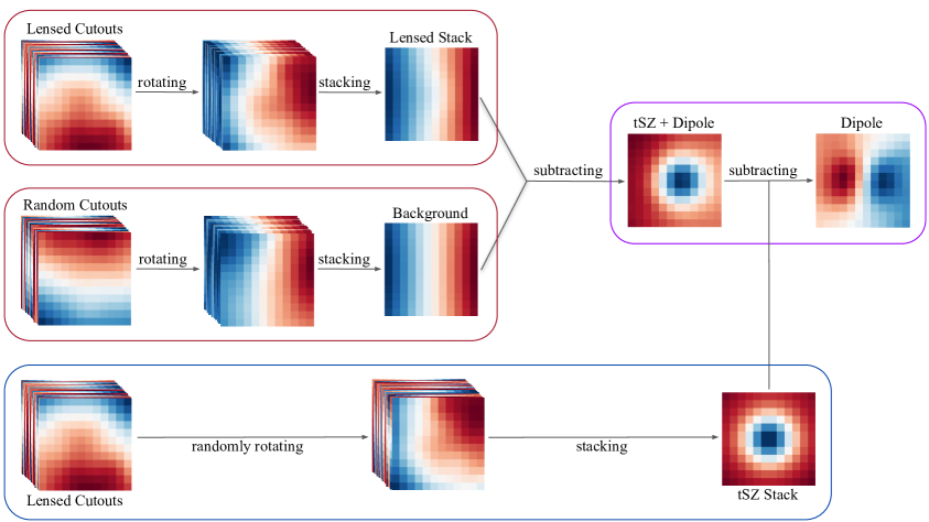
Figure 1: Illustration of the lensing pipeline when applied to CMB temperature mock data. Besides the lensing signal, the cluster-centered cutouts include the cluster-correlated kSZ and tSZ signals. All the cutouts have been smoothed by a Gaussian beam with FWHM = $1^{\prime}$ and contain a white noise level $\Delta T_{\text{white}}=2$ $\mu$K-arcmin. While the kSZ effect cancels out during the stacking process, the rotational-invariant tSZ signal remains in the cluster-lensed stack. An estimate of the mean tSZ signal can be obtained by randomly rotating and stacking the lensed cutouts. This will remove the CMB gradients and lensing dipoles, and thus only leaving the mean tSZ signal. The random rotation process ensures that the gradients between different cutouts are uncorrelated. Additionally, this process can be repeated to obtain a given number of tSZ stacks which can be averaged over to reduce the residual noise within the tSZ stack. Note that, when using CMB polarization data, the additional tSZ mitigation step is not necessary, since foregrounds are largely unpolarized.

Ignoring the effect of foregrounds, an estimate of the mean lensing dipole signal can be obtained from $N_{\text{clus}}$ cluster-centered and $N_{\text{rand}}$ random CMB maps using the following steps [1]:

1. Using the central $(6^{\prime}\times 6^{\prime})$ region in every map, compute the median gradient direction, $\theta_{\nabla T}=\tan^{-1}(\nabla_{y}T/\nabla_{x}T)$, and magnitude, $|\nabla T|=\sqrt{\nabla_{x}T^{2}+\nabla_{y}T^{2}}$.

2. Rotate each map along its gradient direction.

3. Extract central $(6^{\prime}\times 6^{\prime})$ cutouts from the rotated maps.

4. Subtract the median from each cutout.

5. Compute the gradient magnitude weighted cluster-lensed and background stacks, $\boldsymbol{\mathrm{s}}_{\text{clus}}$ and $\boldsymbol{\mathrm{s}}_{\text{bg}}$, respectively.

6. Get an estimate of the mean lensing dipole $\boldsymbol{\mathrm{s}}_{\text{dipole}}$ by subtracting the background stack from the cluster-lensed stack.

Note that the cutout size used in this work is slightly smaller compared to the size used in the original paper: $(6^{\prime}\times 6^{\prime})$ vs $(10^{\prime}\times 10^{\prime})$. Using this smaller cutout size does not degrade the SNR since the majority of the lensing signal comes from regions close to the center. Additionally, the smaller cutout size reduces the number of elements in the covariance matrix. In summary, the individual stacks are given by

$$\boldsymbol{\mathrm{s}}_{\text{clus}} =\frac{\sum_{c}^{N_{\text{clus}}}w_{c}\left[\tilde{\boldsymbol{\mathrm{d}}}_{c}-\langle\tilde{\boldsymbol{\mathrm{d}}}_{c}\rangle\right]}{\sum_{c}^{N_{\text{clus}}}w_{c}}\;,$$ (4.1)

$$\boldsymbol{\mathrm{s}}_{\text{bg}} =\frac{\sum_{r}^{N_{\text{rand}}}w_{r}\left[\tilde{\boldsymbol{\mathrm{d}}}_{r}-\langle\tilde{\boldsymbol{\mathrm{d}}}_{r}\rangle\right]}{\sum_{r}^{N_{\text{rand}}}w_{r}}\;,$$ (4.2)

$$\boldsymbol{\mathrm{s}}_{\text{dipole}} =\boldsymbol{\mathrm{s}}_{\text{clus}}-\boldsymbol{\mathrm{s}}_{\text{bg}}\;.$$ (4.3)

Every rotated cutout, $\tilde{\boldsymbol{\mathrm{d}}}_{i}$, is weighted by the corresponding gradient magnitude, ${\color[rgb]{0,0,0}w_{i}=|\nabla T|_{i}}$, since the dipole signal scales linearly with the CMB background gradient for a given cluster mass. When using real observations, additional weights can be used based on the inverse noise variance $\sigma_{i}^{-2}$ in each cutout, giving a final weight of ${\color[rgb]{0,0,0}w_{i}=|\nabla T|_{i}\sigma_{i}^{-2}}$. Since the noise realizations in our CMB simulations are Gaussian, the noise weights will be the same for each cutout and are neglected in this work.

When working with CMB temperature data, cluster-correlated foregrounds, such as the clusters’ own kSZ and tSZ signals, can significantly bias the mass results. Since the estimator analyzed in this work is based on stacking rotated cutouts, the kSZ effect should not compose a source of bias, as the radial peculiar velocity of a cluster can be positive or negative. The tSZ signal, on the other hand, is rotationally invariant on average, and will be the dominant signal in the background subtracted stack if not accounted for. An estimate of the mean tSZ signal can be obtained from randomly rotated cluster-lensed cutouts, $\tilde{\boldsymbol{\mathrm{d}}}_{c}^{\theta_{\text{rand}}}$, by computing the corresponding gradient weighted stack. The random rotation ensures that any correlations between CMB gradients in different cutouts, which could exist between cluster-centered cutouts that are close to each other on the sphere, will be eliminated. Therefore, the resulting stack will only contain the mean tSZ signal and some residual noise, which can be reduced by averaging over a given number of tSZ stacks obtained from different sets of random rotations:

$$\boldsymbol{\mathrm{s}}_{\text{tSZ}} =\left\langle\frac{\sum_{c}^{N_{\text{clus}}}w_{c}\left[\tilde{{\boldsymbol{\mathrm{d}}}}_{c}^{\theta_{\text{rand}}}-\langle{\tilde{\boldsymbol{\mathrm{d}}}}_{c}^{\theta_{\text{rand}}}\rangle\right]}{\sum_{c}^{N_{\text{clus}}}w_{c}}\right\rangle_{\theta_{\text{rand}}}\;.$$ (4.4)

While we do not explicitly show, we note that the above technique of removing the tSZ signal will also help in removing other cluster-correlated foreground signals, like the emission from member galaxies. The final dipole stack is then given by:

$$\boldsymbol{\mathrm{s}}_{\text{dipole}}=\boldsymbol{\mathrm{s}}_{\text{clus}}-\boldsymbol{\mathrm{s}}_{\text{bg}}-\boldsymbol{\mathrm{s}}_{\text{tSZ}}\;.$$ (4.5)

Fig. 1 illustrates the above steps to extract the lensing dipole from CMB temperature maps.

To reduce the noise penalty in the estimation of the median value of the gradient direction and magnitude, a Wiener filter of the form

$$W_{\ell}=\begin{cases}\frac{C_{\ell}}{C_{\ell}+N_{\ell}}&,\text{ }\ell\leqslant 2000\\ 0&,\text{ }\ell>2000\end{cases}\;$$ (4.6)

is applied to the lensed and random maps. $C_{\ell}$ is the lensed CMB temperature power spectrum and $C_{\ell,\text{noise}}$ refers to the total noise power spectrum of the map. The sharp multipole cut at $\ell=2000$ is used to remove the lensing signal in the cluster-lensed cutouts, which magnifies the background image and leads to a decrease of the CMB gradient [38]. Note that this cut does not degrade the SNR on the gradient measurement since the majority of the CMB gradient comes from $\ell\leqslant 2000$ and the modes beyond those scales are exponentially suppressed due to Silk damping. Thus, this $\ell$-cut should ensure that the random and cluster-lensed cutouts are rotated and weighted in the same way. We compute the gradient within the $(6^{\prime}\times 6^{\prime})$ box around the center of the filtered maps using second order accurate central differences.

5 Statistical and Systematic Analysis

We now perform several statistical and systematic error checks and compare the performance of the estimator to standard CMB-cluster lensing estimators. For these checks, we use $N_{\text{clus}}=25,000$ cutouts for the lensed stack and $N_{\text{rand}}=50,000$ random cutouts for the background stack. We set the redshift to $z=0.7$ for all the clusters. The large number of random maps is used to ensure that the variance in the background stack is negligible. The assumed cluster masses, white noise levels, positional offsets and foregrounds are described below in the individual sections. All the simulations have been smoothed by a Gaussian instrumental beam with FWHM = $1^{\prime}$.

The cluster mass is estimated from the lensing dipole stack by computing the natural logarithm of the likelihood function:

$${\mathrm{\ln}}\mathcal{L}(M|\boldsymbol{\mathrm{s}})=-\frac{1}{2}\left[\boldsymbol{\mathrm{s}}-\boldsymbol{\mathrm{m}}(M)\right]^{T}\boldsymbol{\mathrm{C}}^{-1}\left[\boldsymbol{\mathrm{s}}-\boldsymbol{\mathrm{m}}(M)\right]\;,$$ (5.1)

where $\boldsymbol{\mathrm{s}}$ is the mock dipole vector and $\boldsymbol{\mathrm{m}}(M)$ the mass-dependent model vector. The pixel-pixel covariance matrix $\boldsymbol{\mathrm{C}}$ is estimated using a jackknife re-sampling technique by dividing the $N_{\text{clus}}$ mock observations into $N_{\text{jk}}$ sub-samples:

$$\boldsymbol{\mathrm{C}}=\frac{N_{\text{jk}}-1}{N_{\text{jk}}}\sum_{i=1}^{N_{\text{jk}}}(\boldsymbol{\mathrm{s}}_{i}-\langle\boldsymbol{\mathrm{s}}\rangle)(\boldsymbol{\mathrm{s}}_{i}-\langle\boldsymbol{\mathrm{s}}\rangle)^{T}\;,$$ (5.2)

where $\boldsymbol{\mathrm{s}}_{i}$ is the lensing dipole vector of the $i^{th}$ sub-sample and $\langle\boldsymbol{\mathrm{s}}\rangle$ the average dipole vector of all the sub-samples.

The dipole models are generated using a flat prior for masses selected from a parameter grid ranging from $M\in[0,6]\times 10^{14}\text{ }M_{\odot}$ with a mass resolution of $\Delta M=0.01\times 10^{14}\text{ }M_{\odot}$. The model for each mass is obtained from $N_{\text{clus}}$ fixed CMB simulations, lensed by the cluster with the respective mass. We smooth the maps with a Gaussian beam identical to the one used for the mock data. The background stack for the models is obtained from the corresponding unlensed simulations. We subtract this stack from each lensed stack to get the final lensing dipole models. We add the same noise level to the model simulations that was added to the mock data when estimating the median gradient direction and magnitude. Otherwise, the uncertainty in the determination of the gradient directions will be smaller for the models than for the mock data, leading to a higher amplitude in the model dipoles since the cutouts will be aligned more precisely, and thus to a bias towards lower mass values.

Note that, to create the models, we do not rotate each of the lensed maps by the gradient angles obtained from the corresponding Wiener filtered cutouts, since this introduces a scatter in the likelihood curves. This scatter is due to differences in the uncertainties in the gradient estimation for different cluster masses. Instead, we lens the $i^{th}$ CMB simulation by every mass in the mass bin, infer the gradient angle for each of these lensed simulations, and rotate the maps by the median angle. This ensures that all the different lensed model stacks have been rotated in the same way.

The best-fit mass, $M_{\text{fit}}$, and corresponding $1\sigma$ uncertainty, $\Delta M$, are given as 50th percentile and half the difference between the 16th and 84th percentile of the likelihood function, respectively.

5.1 Pipeline Validation

We begin our analysis by applying the estimator to simulations lensed by different masses to verify whether we can properly recover the input masses. Besides the lensing signal and the instrumental beam, the simulations contain a white noise level $\Delta T_{\text{white}}$ = 2 $\mu$K-arcmin, which roughly corresponds to the noise expected for SPT-3G [17] and S4-Wide [24] experiments. We consider three input masses: $M_{\text{input}}\in[1,2,4]\times 10^{14}\text{ }M_{\odot}$, for which we compute the lensing dipole stacks according to Eq. (4.3). The likelihood curves of 10 individual simulation sets, each containing 2,500 clusters, can be seen as light shaded curves in Fig. 2 for each mass case. The combined likelihood of the 25,000 clusters is shown as thick purple curve. We find median masses and 1$\sigma$ uncertainties of $M_{1\times 10^{14}M_{\odot}}=(1.00\pm 0.01)\times 10^{14}\text{ }M_{\odot}$, $M_{2\times 10^{14}M_{\odot}}=(1.99\pm 0.02)\times 10^{14}\text{ }M_{\odot}$, and $M_{4\times 10^{14}M_{\odot}}=(3.98\pm 0.02)\times 10^{14}\text{ }M_{\odot}$, indicating that, although we can recover the input masses within $1\sigma$ for the considered settings, there seems to be a small systematic shift towards lower masses with increasing cluster mass. The reason for this being that the filter given by Eq. (4.6) does not entirely remove the lensing effect of the cluster, making the rotation process slightly mass dependent. We verify this by redoing the analysis, using the gradient angles estimated from the corresponding underlying unlensed simulations to rotate the lensed mock data and model simulations, and see no mass-depend shift in the recovered masses.

Besides using a smaller value for the multipole cut for the Wiener filter given by Eq. (4.6), a possible method to get unbiased masses for massive clusters would be to inpaint the maps [71, 53] before applying the Wiener filter. Inpainting mitigates the lensing signal, as well as any cluster-correlated foreground signals, by masking the cluster region and filling the corresponding pixel values based on information from surrounding regions using constrained Gaussian realizations. While outside the scope of this work, inpainting the maps before estimating the CMB background gradient orientation constitutes an interesting implementation for a future analysis.

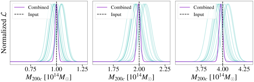
Figure 2: Individual likelihood curves (light shaded turquoise curves) from 10 sets for three mass cases: $M_{\text{input}}\in[1,2,4]\times 10^{14}\ M_{\odot}$. Each set includes 2,500 lensed maps, smoothed by a Gaussian beam with FWHM = $1^{\prime}$ and containing a map noise level of $\Delta T_{\text{white}}=2$ $\mu$K-arcmin. The combined likelihood curve of the 10 sets is shown as solid purple curve. The input mass used for the mock data is highlighted as dashed black line.

5.2 Estimator Comparison

In this section, we compare the fractional mass uncertainty, $\Delta M/M_{\text{input}}$, of the lensing estimator to those obtained for the MLE [29, 30, 31] and QE [38, 45]. The QE estimates the mean cluster mass by exploiting the lensing-induced correlations between previously uncorrelated modes. In the MLE, cluster-lensed CMB templates are fitted to observed CMB maps using the full pixel-space likelihood. For easier comparison, we use the same settings as in Raghunathan et al. [45]: $M=2\times 10^{14}\text{ }M_{\odot}$, $z=0.7$, FWHM = 1^′, and $\Delta T_{\text{white}}\in[0.1,0.5,1,3,5,7]\text{ }\mu$K-arcmin. Since the values in Raghunathan et al. [45] were obtained for $N_{\text{clus}}=100,000$, we scale those values by a factor of $\sqrt{100,000/25,000}=2$. The resulting fractional mass uncertainties can be seen in Fig. 3, together with the values obtained in Raghunathan et al. [45] for the QE and MLE.

The MLE and the estimator analyzed in this work give similar fractional mass uncertainties over the whole noise range. The QE has a similar performance for white noise levels $\Delta T_{\text{white}}\geqslant 3.0$ $\mu$K-arcmin but is outperformed for lower noise levels. For the lowest considered noise level, $\Delta T_{\text{white}}=0.1$ $\mu$K-arcmin, the fractional mass uncertainty of the MLE and the current estimator are improved by $\times 2$ compared to the one obtained for the QE. Since the QE is only a linear approximation, it misses some of the information included in the MLE and the estimator of this work. As demonstrated by [39, 40], using an iterative version of the QE can make it match with the MLE and the current estimator even for low map noise levels.

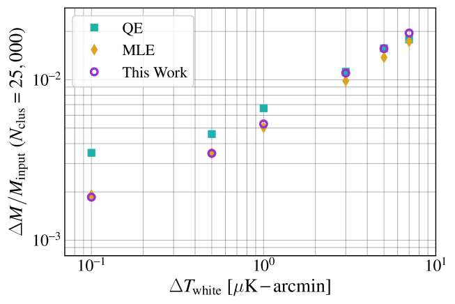
Figure 3: Fractional mass uncertainties for white noise levels $\Delta T_{\text{white}}\in[0.1,0.5,1,3,5,7]\text{ }\mu$K-arcmin using the QE (turquoise squares), the MLE (yellow diamonds), and the estimator of this work (purple circles). The cluster stack is obtained from $N_{\rm clus}=25,000$ lensed cutouts. The three considered estimators have a similar performance for $\Delta T_{\text{white}}\geqslant 3.0$ $\mu$K-arcmin. For lower noise levels, both, the MLE and our estimator, outperform the QE. Specifically, for the case $\Delta T_{\text{white}}=0.1$ $\mu$K-arcmin, the fractional mass uncertainty of the QE is $\times 2$ worse.

5.3 Systematic Biases and Mitigation Strategies

We now turn to the systematic analysis by examining biases due to uncertainties in the cluster positions and the clusters’ own tSZ and kSZ signals. The relative bias due to these systematics is quantified as

$$b_{\rm lens}=\frac{M_{\text{fit}}}{M_{\text{input}}}-1\;.$$ (5.3)

5.3.1 Cluster Positions

To quantify the potential bias due to normal positional uncertainties in the cluster positions, we add a random offset to the position of each cluster, taken from a Gaussian distribution, $N(0,\sigma_{\text{offset}})$, with a standard deviation $\sigma_{\text{offset}}\in[0^{\prime},0.25^{\prime},0.5^{\prime},0.75^{\prime},1^{\prime},1.25^{\prime},1.5^{\prime},1.75^{\prime},2^{\prime}]$. We use a cluster mass $M=2\times 10^{14}\text{ }M_{\odot}$ and a white noise level $\Delta T_{\text{white}}=2$ $\mu$K-arcmin. Fig. 4 shows the biases due to the centroid shifts. Since the clusters are all shifted from the true center of the maps, the final cluster stack will have a lower dipole amplitude since the lensing signal got smoothed out to some extent, which leads to a bias towards lower masses. Specifically, we find a bias of $b_{\rm lens}=-0.05\pm 0.01$ for $\sigma_{\text{offset}}=0.5^{\prime}$, which is a typical offset between the SZ centers in CMB data and the red brightest cluster galaxy in optical and near-infrared data [72]. Having an estimate of the expected centroid shift for the considered galaxy cluster survey, $\sigma_{\text{expected}}$, the bias can be mitigated by shifting the lensed model simulations according to a Gaussian distribution $N(0,\sigma_{\text{expected}})$. While this increases the mass uncertainties, we find that it is $\lesssim 10\%$ for the cases $\sigma_{\text{offset}}\lesssim 0.5^{\prime}$, and thus negligible (see Fig. 4). For the typical case of $\sigma_{\text{offset}}=0.5^{\prime}$, we find a relative bias value $b_{\rm lens}=-0.01\pm 0.01$ after correction.

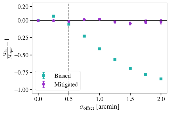
Figure 4: Bias analysis due to uncertainties in the cluster positions for 25,000 clusters. Unaccounted positional uncertainties in the data will lead to a bias towards lower masses (turquoise squares). For a typical positional offset of $0.5^{\prime}$ expected in SZ surveys [72], marked with a dashed black line, we find a bias $b_{\rm lens}=-0.05\pm 0.01$. Accounting for the uncertainties in the models helps mitigating the bias at the cost of an increased mass error (purple points), which is $\lesssim 10\%$ for $\sigma_{\text{offset}}\lesssim 0.5^{\prime}$, and hence negligible.

5.3.2 Foreground Bias

While cluster-correlated signals are largely unpolarized and were not a concern for the results in R19, they can have a large impact on the lensing mass reconstruction when using CMB temperature data. In this section, we analyze the effects of the cluster-correlated kSZ and tSZ signals on the final mass result both separately and together. For this, we add $(60^{\prime}\times 60^{\prime})$ kSZ and/or $(60^{\prime}\times 60^{\prime})$ 150 GHz tSZ maps, obtained from Agora simulations [60], to the cluster-lensed maps. Since we are using $25,000$ lensed cutouts in this analysis, we pick clusters in the mass range $M_{200c}\in[1.25,1.69]\times 10^{14}\text{ }M_{\odot}$ and redshift range $z\in[0.6,0.8]$ to get a large enough sample of kSZ and tSZ simulations. For this section, we set the cluster mass to $M_{200c}=1.47\times 10^{14}\text{ }M_{\odot}$ and use a redshift $z=0.7$ for the cluster-lensed maps. As in the previous section, we add a white noise level $\Delta T_{\text{white}}=2$ $\mu$K-arcmin to all the maps.

Since the clusters can either have a positive or negative kSZ signal depending on their peculiar velocity relative to us, the estimator is naturally immune to kSZ-induced lensing biases when we stack the lensing signal from multiple clusters. However, including the kSZ signal slightly increases the variance in the final lensing dipole stack. Specifically, the mass uncertainties are increased by a factor of 1.2 compared to the baseline case.

On the other hand, the tSZ signal introduces significant issues. For example, when we compare the model dipole stack to the mock data stack in the presence of the tSZ signal, we get a Probability-To-Exceed (PTE) value $\simeq 0$, since the final stack is dominated by the mean tSZ signal of all the clusters. This improves and matches the baseline and kSZ cases after applying the tSZ mitigation step (see Eq. (4.4) and (4.5)). In that case, we find a relative bias $b_{\rm lens}=-0.01\pm 0.02$, indicating that the tSZ contamination has been effectively reduced. However, the tSZ mitigation step increases the mass uncertainty by a factor of $\sim 2$ compared to the baseline case. As expected, we find similar results when considering the impact of both, the kSZ and tSZ signals, after applying the tSZ mitigation step. Considering both the impact due to uncertainties in the cluster positions (using $\sigma_{\text{offset}}=0.5^{\prime}$), as well as the kSZ and tSZ signals after applying the tSZ mitigation step, we find the mass uncertainty to increase by $\sim 2.5$ compared to the baseline case.

Similar to §5.1, we note that the gradient direction estimation could be contaminated by the tSZ signal for massive clusters. This can be mitigated using the techniques mentioned in §5.1, or by using a tSZ-nulled map for the gradient estimation. Since the SNR of the CMB for modes $\ell<2000$ is extremely high for current and future CMB surveys, the noise enhancement due to tSZ nulling will have negligible impact on the final lensing SNR.

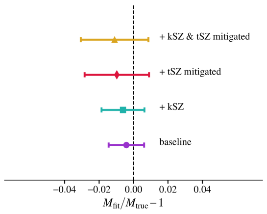
Figure 5: Bias analysis due to cluster-correlated kSZ and tSZ signals. The underlying CMB realizations have been fixed for all the cases to highlight the impact of the foregrounds on the mass estimates. The kSZ signal (turquoise square) only acts as an additional source of variance, while the tSZ signal has to be mitigated to get an unbiased mass estimate (red diamond).

6 Lensing SNR Forecasts

The next generation CMB experiments are expected to improve the CMB-cluster lensing-based mass calibration substantially [73, 36, 74]. In this final section, we forecast the lensing SNR for SPT-3G and three upcoming experiments.

The mock data for each experiment includes the CMB lensing signal along with residual noise and foregrounds, calculated using Eq. (3.7) and the frequency bands and noise levels given in Table 1 and 2. To make the forecasts realistic, we also include the cluster-correlated kSZ and tSZ signals. Note that, compared to the foreground signals in §5.3.2, the tSZ signals will be slightly down-weighted here because of the frequency dependent ILC weights given by Eq. (3.5).

6.1 Experiments

The CMB experiments considered in this work include

• SPT-3G: The South Pole Telescope (SPT) [75] is a 10-meter telescope located at the Amundsen–Scott South Pole Station in Antarctica. SPT-3G [16, 17, 18] is the third generation receiver operating on SPT, dedicated to high-resolution observations of the CMB. The receiver contains $\sim$16,000 polarization-sensitive detectors, providing arcminute-scale resolution maps of the CMB using 95 GHz, 150 GHz, and 220 GHz frequency band centers. SPT-3G was installed in 2017 and started a 6-year 1500 deg² survey in February 2018. The expected number of clusters is 7,000 [76].

• SO: The Simons Observatory (SO) [20] is a next-generation CMB observatory located in the Atacama Desert in Northern Chile inside the Chajnator Science Preserve at 5,200 meters. It consists of one 6-meter diameter large-aperture telescope (SO-LAT) measuring CMB temperature and polarization. The observed fraction of the sky will be 40% for the LAT instrument. The frequency band centers used for all the instruments are 27 GHz, 39 GHz, 93 GHz, 145 GHz, 225 GHz and 280 GHz, and the expected number of cluster is 25,000 [74, 20, 76].

• FYST: The Fred Young Submillimeter Telescope (FYST)[21, 22], previously known as CCAT-prime, is a 6-meter diameter telescope located at 5,600 meters on the Cerro Chajnantor mountain in the Atacama Desert of Northern Chile. FYST will cover 35% of the sky area using 220 GHz, 280 GHz, 350 GHz, and 410 GHz frequency bands. Combining its submillimeter imaging with the millimeter imaging of SO will allow precise separation of foreground dust emission from the CMB signal.

• S4-Wide: The fourth-generation ground-based CMB experiment (S4-Wide) [23, 24] will be operating at the South Pole and in the Chajnantor Plateau in the Atacama desert in Northern Chile . The anticipated year for the start of the survey is 2029. The South Pole telescopes will conduct an ultra-deep survey (S4-Ultra deep), covering 3% of the sky, while the Atacama telescopes will conduct a wide (S4-Wide) and a deep (S4-Deep) survey with a 65% sky coverage. For this work, we will only consider S4-Wide, which will use 27 GHz, 39 GHz, 93 GHz, 145 GHz, 225 GHz and 280 GHz frequency band centers. The expected number of cluster is 100,000 [73, 74, 77, 76].

Table 1 lists the instrumental beams and the detector noise levels $\Delta T_{\text{white}}$ of each frequency band for the four experiments. The parameters governing the atmospheric noise ($\ell_{\text{knee}}$, $\alpha_{\text{knee}}$, and $\Delta T_{\text{red}}$) are listed in Table 2. While the four high-frequency (HF) channels of FYST cannot be used independently for CMB science, they can be combined with the SO frequency channels to reduce the residual noise in the final maps.

Table 1: Instrumental beam and detector noise specifications for the current and future experiments considered in this work.

Frequency [GHz]	Beam [arcminutes]				$\Delta T_{\rm white}$ [$\mu$K-arcmin]
	SPT-3G	SO	SO + FYST	S4-Wide	SPT-3G	SO	SO + FYST	S4-Wide
27	-	7.4			-	52.1		21.5
39		5.1				27.1		11.9
93	-	2.2			-	5.8		1.9
95	1.7	-			3.0	-
145	-	1.4			-	6.5		2.1
150	1.2	-			2.2	-
220	1.0	-	0.95	-	8.8	-	14.6	-
225	-	1.0			-	15.0		6.9
280$\ast$	-	0.9	0.75	0.7	-	37.0	27.5	16.8
350		-	0.58	-		-	104.8	-
410			0.50				376.6

• For the 280 GHz band that overlaps for SO and FYST, we combine the noise power spectra using inverse
  variance weighting.

Table 2: Atmospheric noise specifications for the current and future experiments considered in this work.

Frequency	$\ell_{\rm knee}$			$\alpha_{\rm knee}$			$\Delta T_{\rm red}$ [$\mu$K-arcmin]
[GHz]	SPT-3G	SO	S4-Wide	SPT-3G	SO	S4-Wide	SO	SO + FYST
27	-	1000	415	-	-3.5	-3.5	6.1
39			391				3.8
93$\ast$	1200		1932	-3			9.3
145$\ast$	2200		3917	-4			23.8
225$\ast$	2300		6740	-4			80.0	434.8
280	-		6792	-			108.0	1140.2
350		-			-		-	5648.8
410								14174.2

• For simplicity, we do not include all the frequency bands in this table by assuming 93 $\leftrightarrow$ 95 GHz, 145 $\leftrightarrow$ 150 GHz, and 220 $\leftrightarrow$ 225 GHz.

6.2 Results

As in the previous section, we use $N_{\text{rand}}=50,000$ random cutouts for the background stack. For the lensed stacks, we use the expected cluster number for each experiment: $N_{\text{clus}}^{\rm SPT-3G}=7,000$, $N_{\text{clus}}^{\rm SO}$ = $N_{\text{clus}}^{\rm SO+FYST}=25,000$, and $N_{\text{clus}}^{\rm S4-Wide}=100,000$. We use a cluster mass $M=1.47\times 10^{14}\text{ }M_{\odot}$ and a cluster redshift $z=0.7$, since this is the mean mass and redshift used to extract the kSZ and tSZ signals from Agora simulations. After adding a Gaussian realization of the expected ILC residual noise power spectrum (see Fig. 6), and the kSZ and ILC weighted tSZ maps to the cluster-lensed simulations, we smooth each map by a Gaussian instrumental beam with a FWHM corresponding to the beam at the 145 GHz or 150 GHz channel of the experiments given in Table 1. As was done in §5.3.2, we get an estimate of the mean tSZ signal using Eq. (4.4) and compute the lensing dipole according to Eq. (4.5).

The lensing SNR for each experiment is obtained as

$$\text{SNR}=\sqrt{\Delta\chi^{2}}=\sqrt{2\left[{\mathrm{\ln}}\mathcal{L}(M=M_{\text{fit}})-{\mathrm{\ln}}\mathcal{L}(M=0)\right]}\;.$$ (6.1)

Specifically, we find SNR_SPT-3G = 15.1 (6.6% mass constraints), SNR_SO = 24.4 (4.1% mass constraints), SNR_SO+FYST = 25.6 (3.9% mass constraints), and SNR_S4-Wide = 57.0 (1.8% mass constraints). The resulting SNR values are shown in Fig. 7. Adding the HF information from FYST to SO has little impact on the lensing SNR. However, we note that the HF channels can give a better handle on the foregrounds for cluster detection. It is expected that SO will detect nearly four times more clusters than SPT-3G due to a much larger sky coverage, resulting in a SNR value roughly twice the value of SPT-3G. On the other hand, S4-Wide will have a $\times 14$ larger cluster sample than SPT-3G, which leads to a significantly higher lensing SNR (roughly $\times 4$ higher than for SPT-3G).

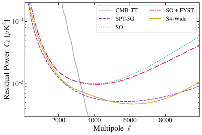
Figure 6: ILC noise power spectra for the CMB experiments considered in this work. Also shown is the CMB temperature power spectrum (solid gray line). SPT-3G (dashed purple line) and S4-Wide (long-dashed yellow line) are roughly similar since they are dominated by the residual CIB signals which set a noise floor. The residual power for SO (dotted turquoise line) can be slightly decreased using the additional HF channels from FYST (dash-dotted red line).

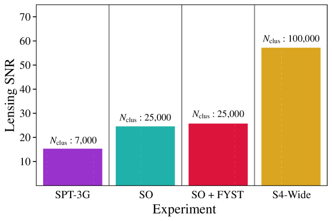
Figure 7: Expected CMB-cluster lensing SNR values for current (SPT-3G) and future experiments (SO, SO + FYST, S4-Wide). The SNR values for SO and SO + FYST are nearly twice as high as the one for SPT-3G. For S4-Wide, the sensitivity is $\times 4$ higher compared to SPT-3G. However, this increase in the lensing SNR for future experiments is driven by the much larger sky coverage providing more clusters to stack. We note that the sensitivity for a single cluster is roughly the same for both SPT-3G and S4-Wide.

7 Conclusions

In this work, we extended the cluster lensing estimator developed in R19 to CMB temperature data. We compared the performance of the estimator to the MLE and QE, finding that the SNR of the current estimator matches the MLE for all map noise levels. We also analyzed the impact of the cluster-correlated kSZ and tSZ signals. Unlike other CMB-cluster lensing estimators, we showed that the kSZ signal does not introduce a bias and only acts as an additional source of variance. We also demonstrated that the bias induced by the tSZ signal can be trivially mitigated by subtracting a tSZ estimate obtained from the cluster-lensed cutouts themselves. When working with real data, this technique will also help in removing the bias due to the CIB, as well as any other foregrounds correlated with the clusters under study.

We did not include the effects of the rotational kSZ [78, 79, 80, 81] or the moving-lens effect [82, 83], which are also expected to produce a dipole signal. However, the orientation of the dipole will be aligned along the direction of the cluster rotation in the former and the direction of the large-scale velocity field in the latter, which are both not correlated with the direction of the background CMB gradient. As a result, these signals tend to dilute in our final stack. Moreover, the amplitude of these signals are expected to be similar in level or smaller than cluster lensing for the typical clusters considered in this work. Therefore, the level of bias should be negligible compared to the statistical errors.

We also studied the impact of mis-centering and found a bias $b_{\rm lens}=-0.05\pm 0.01$ for realistic positional uncertainties in the cluster location ($\sigma_{\text{offset}}=0.5^{\prime}$). However, this bias can be easily mitigated by including the positional uncertainties in the model lensing dipoles with a negligible degradation of the lensing SNR for $\sigma_{\text{offset}}\lesssim 0.5^{\prime}$.

Finally, we presented forecasts for the expected lensing SNR for current and future CMB surveys. We predict cluster mass uncertainties of 6.6% for SPT-3G with 7,000 clusters, 4.1% for SO and 3.9% for SO + FYST with 25,000 clusters, and 1.8% for S4-Wide with 100,000 clusters. The additional HF bands from FYST did not significantly increase the lensing SNR of SO. However, they might be useful to handle the contamination of the tSZ signal due to dusty galaxies for cluster detection.

The lensing estimator presented in this work can also be applied for mass calibration of clusters identified from optical or X-ray surveys.

References

- Raghunathan et al. [2019a] S. Raghunathan, S. Patil, E. Baxter, B. A. Benson, L. E. Bleem, T. M. Crawford, G. P. Holder, T. McClintock, C. L. Reichardt, T. N. Varga, et al., Physical Review Letters 123, 181301 (2019a), arXiv:1907.08605 [astro-ph.CO] .
- Bleem et al. [2015] L. E. Bleem, B. Stalder, T. de Haan, K. A. Aird, S. W. Allen, D. E. Applegate, M. L. N. Ashby, M. Bautz, M. Bayliss, B. A. Benson, et al., The Astrophysical Journal Supplement Series 216, 27 (2015), arXiv:1409.0850 [astro-ph.CO] .
- Planck Collaboration et al. [2016] Planck Collaboration, P. A. R. Ade, N. Aghanim, M. Arnaud, M. Ashdown, J. Aumont, C. Baccigalupi, A. J. Banday, R. B. Barreiro, J. G. Bartlett, et al., A&A 594, A24 (2016), arXiv:1502.01597 [astro-ph.CO] .
- Huang et al. [2020] N. Huang, L. E. Bleem, B. Stalder, P. A. R. Ade, S. W. Allen, A. J. Anderson, J. E. Austermann, J. S. Avva, J. A. Beall, A. N. Bender, et al., The Astronomical Journal 159, 110 (2020), arXiv:1907.09621 [astro-ph.CO] .
- Bleem et al. [2020] L. E. Bleem, S. Bocquet, B. Stalder, M. D. Gladders, P. A. R. Ade, S. W. Allen, A. J. Anderson, J. Annis, M. L. N. Ashby, J. E. Austermann, et al., The Astrophysical Journal Supplement Series 247, 25 (2020), arXiv:1910.04121 [astro-ph.CO] .
- Hilton et al. [2021] M. Hilton, C. Sifón, S. Naess, M. Madhavacheril, M. Oguri, E. Rozo, E. Rykoff, T. M. C. Abbott, S. Adhikari, M. Aguena, et al., The Astrophysical Journal Supplement Series 253, 3 (2021), arXiv:2009.11043 [astro-ph.CO] .
- Mantz et al. [2010] A. Mantz, S. W. Allen, H. Ebeling, D. Rapetti, and A. Drlica-Wagner, MNRAS 406, 1773 (2010), arXiv:0909.3099 [astro-ph.CO] .
- Rozo et al. [2010] E. Rozo, R. H. Wechsler, E. S. Rykoff, J. T. Annis, M. R. Becker, A. E. Evrard, J. A. Frieman, S. M. Hansen, J. Hao, D. E. Johnston, B. P. Koester, T. A. McKay, E. S. Sheldon, and D. H. Weinberg, ApJ 708, 645 (2010), arXiv:0902.3702 [astro-ph.CO] .
- Rykoff et al. [2014] E. S. Rykoff, E. Rozo, M. T. Busha, C. E. Cunha, A. Finoguenov, A. Evrard, J. Hao, B. P. Koester, A. Leauthaud, B. Nord, M. Pierre, R. Reddick, T. Sadibekova, E. S. Sheldon, and R. H. Wechsler, ApJ 785, 104 (2014), arXiv:1303.3562 [astro-ph.CO] .
- von der Linden et al. [2014] A. von der Linden, M. T. Allen, D. E. Applegate, P. L. Kelly, S. W. Allen, H. Ebeling, P. R. Burchat, D. L. Burke, D. Donovan, R. G. Morris, R. Blandford, T. Erben, and A. Mantz, MNRAS 439, 2 (2014), arXiv:1208.0597 [astro-ph.CO] .
- Bartelmann [1996] M. Bartelmann, A&A 313, 697 (1996), arXiv:astro-ph/9602053 [astro-ph] .
- Zubeldia and Challinor [2019] Í. Zubeldia and A. Challinor, MNRAS 489, 401 (2019), arXiv:1904.07887 [astro-ph.CO] .
- Bocquet et al. [2019] S. Bocquet, J. P. Dietrich, T. Schrabback, L. E. Bleem, M. Klein, S. W. Allen, D. E. Applegate, M. L. N. Ashby, M. Bautz, and M. Bayliss, ApJ 878, 55 (2019), arXiv:1812.01679 [astro-ph.CO] .
- To et al. [2021] C. To, E. Krause, E. Rozo, H. Wu, D. Gruen, R. H. Wechsler, T. F. Eifler, E. S. Rykoff, M. Costanzi, M. R. Becker, et al., Physical Review Letters 126, 141301 (2021), arXiv:2010.01138 [astro-ph.CO] .
- Costanzi et al. [2021] M. Costanzi, A. Saro, S. Bocquet, T. M. C. Abbott, M. Aguena, S. Allam, A. Amara, J. Annis, S. Avila, D. Bacon, et al., Physical Review D. 103, 043522 (2021), arXiv:2010.13800 [astro-ph.CO] .
- Benson et al. [2014] B. A. Benson, P. A. R. Ade, Z. Ahmed, S. W. Allen, K. Arnold, J. E. Austermann, A. N. Bender, L. E. Bleem, J. E. Carlstrom, C. L. Chang, et al., in Millimeter, Submillimeter, and Far-Infrared Detectors and Instrumentation for Astronomy VII, Society of Photo-Optical Instrumentation Engineers (SPIE) Conference Series, Vol. 9153, edited by W. S. Holland and J. Zmuidzinas (2014) p. 91531P, arXiv:1407.2973 [astro-ph.IM] .
- Bender et al. [2018] A. N. Bender, P. A. R. Ade, Z. Ahmed, A. J. Anderson, J. S. Avva, K. Aylor, P. S. Barry, R. Basu Thakur, B. A. Benson, L. S. Bleem, et al., in Millimeter, Submillimeter, and Far-Infrared Detectors and Instrumentation for Astronomy IX, Society of Photo-Optical Instrumentation Engineers (SPIE) Conference Series, Vol. 10708, edited by J. Zmuidzinas and J.-R. Gao (2018) p. 1070803, arXiv:1809.00036 [astro-ph.IM] .
- Sobrin et al. [2022] J. A. Sobrin, A. J. Anderson, A. N. Bender, B. A. Benson, D. Dutcher, A. Foster, N. Goeckner-Wald, J. Montgomery, A. Nadolski, A. Rahlin, et al., The Astrophysical Journal Supplement Series 258, 42 (2022), arXiv:2106.11202 [astro-ph.IM] .
- Henderson et al. [2016] S. W. Henderson, R. Allison, J. Austermann, T. Baildon, N. Battaglia, J. A. Beall, D. Becker, F. De Bernardis, J. R. Bond, E. Calabrese, et al., Journal of Low Temperature Physics 184, 772 (2016), arXiv:1510.02809 [astro-ph.IM] .
- Ade et al. [2019] P. Ade, J. Aguirre, Z. Ahmed, S. Aiola, A. Ali, D. Alonso, M. A. Alvarez, K. Arnold, P. Ashton, J. Austermann, et al., JCAP 2019, 056 (2019), arXiv:1808.07445 [astro-ph.CO] .
- Choi et al. [2020] S. K. Choi, J. Austermann, K. Basu, N. Battaglia, F. Bertoldi, D. T. Chung, N. F. Cothard, S. Duff, C. J. Duell, P. A. Gallardo, et al., Journal of Low Temperature Physics 199, 1089 (2020), arXiv:1908.10451 [astro-ph.IM] .
- CCAT-Prime Collaboration et al. [2023] CCAT-Prime Collaboration, M. Aravena, J. E. Austermann, K. Basu, N. Battaglia, B. Beringue, F. Bertoldi, F. Bigiel, J. R. Bond, P. C. Breysse, et al., The Astrophysical Journal Supplement Series 264, 7 (2023), arXiv:2107.10364 [astro-ph.CO] .
- Abazajian et al. [2016] K. N. Abazajian, P. Adshead, Z. Ahmed, S. W. Allen, D. Alonso, K. S. Arnold, C. Baccigalupi, J. G. Bartlett, N. Battaglia, B. A. Benson, et al., arXiv e-prints , arXiv:1610.02743 (2016), arXiv:1610.02743 [astro-ph.CO] .
- Abazajian et al. [2019] K. Abazajian, G. Addison, P. Adshead, Z. Ahmed, S. W. Allen, D. Alonso, M. Alvarez, A. Anderson, K. S. Arnold, C. Baccigalupi, et al., arXiv e-prints , arXiv:1907.04473 (2019), arXiv:1907.04473 [astro-ph.IM] .
- Laureijs et al. [2011] R. Laureijs, J. Amiaux, S. Arduini, J. L. Auguères, J. Brinchmann, R. Cole, M. Cropper, C. Dabin, L. Duvet, A. Ealet, et al., arXiv e-prints , arXiv:1110.3193 (2011), arXiv:1110.3193 [astro-ph.CO] .
- LSST Science Collaboration et al. [2009] LSST Science Collaboration, P. A. Abell, J. Allison, S. F. Anderson, J. R. Andrew, J. R. P. Angel, L. Armus, D. Arnett, S. J. Asztalos, T. S. Axelrod, et al., arXiv e-prints , arXiv:0912.0201 (2009), arXiv:0912.0201 [astro-ph.IM] .
- Predehl et al. [2010] P. Predehl, R. Andritschke, H. Böhringer, W. Bornemann, H. Bräuninger, H. Brunner, M. Brusa, W. Burkert, V. Burwitz, N. Cappelluti, et al., in Space Telescopes and Instrumentation 2010: Ultraviolet to Gamma Ray, Society of Photo-Optical Instrumentation Engineers (SPIE) Conference Series, Vol. 7732, edited by M. Arnaud, S. S. Murray, and T. Takahashi (2010) p. 77320U, arXiv:1001.2502 [astro-ph.CO] .
- Hoekstra et al. [2013] H. Hoekstra, M. Bartelmann, H. Dahle, H. Israel, M. Limousin, and M. Meneghetti, Space Science Reviews 177, 75 (2013), arXiv:1303.3274 [astro-ph.CO] .
- Seljak and Zaldarriaga [2000] U. Seljak and M. Zaldarriaga, ApJ 538, 57 (2000), arXiv:astro-ph/9907254 [astro-ph] .
- Dodelson [2004] S. Dodelson, Physical Review D. 70, 023009 (2004), arXiv:astro-ph/0402314 [astro-ph] .
- Lewis and King [2006] A. Lewis and L. King, Physical Review D. 73, 063006 (2006), arXiv:astro-ph/0512104 [astro-ph] .
- Holder and Kosowsky [2004] G. Holder and A. Kosowsky, ApJ 616, 8 (2004), arXiv:astro-ph/0401519 [astro-ph] .
- Vale et al. [2004] C. Vale, A. Amblard, and M. White, New Astronomy 10, 1 (2004), arXiv:astro-ph/0402004 [astro-ph] .
- Horowitz et al. [2019] B. Horowitz, S. Ferraro, and B. D. Sherwin, MNRAS 485, 3919 (2019), arXiv:1710.10236 [astro-ph.CO] .
- Baxter et al. [2015] E. J. Baxter, R. Keisler, S. Dodelson, K. A. Aird, S. W. Allen, M. L. N. Ashby, M. Bautz, M. Bayliss, B. A. Benson, L. E. Bleem, et al., ApJ 806, 247 (2015), arXiv:1412.7521 [astro-ph.CO] .
- Raghunathan et al. [2017] S. Raghunathan, S. Patil, E. J. Baxter, F. Bianchini, L. E. Bleem, T. M. Crawford, G. P. Holder, A. Manzotti, and C. L. Reichardt, JCAP 2017, 030 (2017), arXiv:1705.00411 [astro-ph.CO] .
- Maturi et al. [2005] M. Maturi, M. Bartelmann, M. Meneghetti, and L. Moscardini, A&A 436, 37 (2005), arXiv:astro-ph/0408064 [astro-ph] .
- Hu et al. [2007] W. Hu, S. DeDeo, and C. Vale, New Journal of Physics 9, 441 (2007), arXiv:astro-ph/0701276 [astro-ph] .
- Yoo and Zaldarriaga [2008] J. Yoo and M. Zaldarriaga, Physical Review D. 78, 083002 (2008), arXiv:0805.2155 [astro-ph] .
- Yoo et al. [2010] J. Yoo, M. Zaldarriaga, and L. Hernquist, Physical Review D. 81, 123006 (2010), arXiv:1005.0847 [astro-ph.CO] .
- Melin and Bartlett [2015] J.-B. Melin and J. G. Bartlett, A&A 578, A21 (2015), arXiv:1408.5633 [astro-ph.CO] .
- Gupta and Reichardt [2021] N. Gupta and C. L. Reichardt, ApJ 923, 96 (2021), arXiv:2005.13985 [astro-ph.CO] .
- Madhavacheril et al. [2015] M. Madhavacheril, N. Sehgal, R. Allison, N. Battaglia, J. R. Bond, E. Calabrese, J. Caligiuri, K. Coughlin, D. Crichton, R. Datta, et al., Physical Review Letters 114, 151302 (2015), arXiv:1411.7999 [astro-ph.CO] .
- Geach and Peacock [2017] J. E. Geach and J. A. Peacock, Nature Astronomy 1, 795 (2017), arXiv:1707.09369 [astro-ph.CO] .
- Raghunathan et al. [2018] S. Raghunathan, F. Bianchini, and C. L. Reichardt, Physical Review D. 98, 043506 (2018), arXiv:1710.09770 [astro-ph.CO] .
- Baxter et al. [2018] E. J. Baxter, S. Raghunathan, T. M. Crawford, P. Fosalba, Z. Hou, G. P. Holder, Y. Omori, S. Patil, E. Rozo, T. M. C. Abbott, et al., MNRAS 476, 2674 (2018), arXiv:1708.01360 [astro-ph.CO] .
- Raghunathan et al. [2019b] S. Raghunathan, S. Patil, E. Baxter, B. A. Benson, L. E. Bleem, T. L. Chou, T. M. Crawford, G. P. Holder, T. McClintock, C. L. Reichardt, et al., ApJ 872, 170 (2019b), arXiv:1810.10998 [astro-ph.CO] .
- Geach et al. [2019] J. E. Geach, J. A. Peacock, A. D. Myers, R. C. Hickox, M. C. Burchard, and M. L. Jones, ApJ 874, 85 (2019), arXiv:1902.06955 [astro-ph.GA] .
- Madhavacheril et al. [2020] M. S. Madhavacheril, C. Sifón, N. Battaglia, S. Aiola, S. Amodeo, J. E. Austermann, J. A. Beall, D. T. Becker, J. R. Bond, et al., The Astrophysical Journal Letters 903, L13 (2020), arXiv:2009.07772 [astro-ph.CO] .
- Sunyaev and Zeldovich [1970] R. A. Sunyaev and Y. B. Zeldovich, Astrophysics and Space Science 7, 3 (1970).
- Sunyaev and Zeldovich [1980] R. A. Sunyaev and Y. B. Zeldovich, MNRAS 190, 413 (1980).