On the tubular eigenvalues of third-order tensors

Abstract.

This paper introduces the notion of tubular eigenvalues of third-order tensors with respect to T-products of tensors and analyzes their properties. A focus of the paper is to discuss relations between tubular eigenvalues and two alternative definitions of eigenvalue for third-order tensors that are known in the literature, namely eigentuple and T-eigenvalue. In addition, it establishes a few results on tubular spectra of tensors which can be exploited to analyze the convergence of tubular versions of iterative methods for solving tensor equations.

Keywords: Multilinear algebra, tensor, T-product, T-eigenvalue, eigentuple, Iterative method.
2010 AMS Subject Classification: 15A69, 65F10.

^§Department of Mathematics, Vali-e-Asr University of Rafsanjan, P.O. Box 518, Rafsanjan, Iran
e-mails: f.beik@vru.ac.ir; beik.fatemeh@gmail.com

^‡Computer Science & Engineering, University of Minnesota, Twin Cities, USA
e-mail: saad@umn.edu

1. Introduction and preliminaries

Throughout this paper, we consider third-order tensors denoted by calligraphic letters, e.g., $\mathscr{X}$, which are members of $\mathbb{C}^{n\times m\times p}$. Associated with such tensors, we denote by $X_{k}\;\;{\rm for}\quad k=1,2,\ldots,p$ the matrix of order $n\times m$ obtained by fixing the last index to $k$. This matrix is commonly referred to as a frontal slice. The T-product was first introduced in [12] as a tensor-tensor multiplication. When working with high-dimensional data, this product was found to be a particularly useful tool when compared with matricization, see [8, 9, 10, 11, 19, 23] and the references therein.

Generalizing the concept of eigenvalues from matrices to tensors has also been considered using T-products. For instance, Braman [3] defined the eigenvalue of $n\times n\times n$ tensor as a vector rather than a scalar. The authors of [18] defined the concepts of eigentuples and eigenmatrices of $n\times n\times p$ tensors as an extension of the idea used in [3]. Recently, a few publications were devoted to the study of eigenvalues of $n\times n\times p$ tensors as scalars [14, 16, 17] which are called T-eigenvalues of tensors. In this paper, we consider the eigenvalue of an $n\times n\times p$ tensor as an $1\times 1\times p$ tensor called a tubular eigenvalue. The properties of the above mentioned types of eigenvalues are analyzed in detail. In addition, the paper will aim to present a number of relations between tubular eigenvalues and T-eigenvalues as well as eigentuples. It should be noted that there has been an increased interest in applying iterative methods for solving tensor equations with respect to T-product, see, e.g., [5, 6, 15, 20, 19, 21]. Therefore, we also establish a few theoretical results that can be utilized to analyze the convergence of iterative methods with respect to tubular eigenvalues and point out the benefits of working with tubular eigenvalues instead of T-eigenvalues.

The remainder of this paper is organized as follows. The end of this section presents the notations, definitions, and a few preliminaries used throughout the paper. The definition and properties of the tubular eigenvalues are presented in Section 2. Section 3, introduces the notion of tubular spectral radius and establishes some convergence results of (non)-stationary iterative methods. The paper ends with a few concluding remarks in Section 4.

1.1. Definitions, notations and properties

The scalar Frobenius norm of a tensor $\mathscr{X}\in\mathbb{C}^{n\times m\times p}$ is given by (see [13])

$$\left\|\mathscr{X}\right\|^{2}_{F}={\sum\limits_{i_{1}=1}^{n}{\sum\limits_{i_{2}=1}^{m}{\sum\limits_{i_{3}=1}^{p}{|\mathscr{X}_{i_{1}i_{2}i_{3}}|^{2}}}}}.$$

The scalar Frobenius inner product of two tensors $\mathscr{X},\mathscr{Y}\in\mathbb{C}^{n\times m\times p}$ of the same shape is defined by

$$\left\langle{\mathscr{X},\mathscr{Y}}\right\rangle_{F}=\sum\limits_{i_{1}=1}^{n}\sum\limits_{i_{2}=1}^{m}\sum\limits_{i_{3}=1}^{p}{\rm conj}({\mathscr{X}_{i_{1}i_{2}i_{3}}})\mathscr{Y}_{i_{1}i_{2}i_{3}}$$

where ${\rm conj}({\mathscr{X}_{i_{1}i_{2}i_{3}}})$ stands for the complex conjugate of $\mathscr{X}_{i_{1}i_{2}i_{3}}$

A $1\times 1\times p$ tensor $\mathscr{V}$ is called a tubular tensor of length $p$. To a vector $v\ \in\mathbb{C}^{p}$ with components $v_{1},v_{2},\ldots,v_{p}$, we can associate a tubular tensor $\mathscr{V}$, in a canonical way by setting $\mathscr{V}_{11j}=v_{j}$ for $j=1,2,\ldots,p$. Note that we can always associate a vector $v$ to a tubular tensor $\mathscr{V}$ by defining the $j$th entry of $v$ to be $\mathscr{V}_{11j}$ for $j=1,2,\ldots,n$. Throughout the paper, the tubular tensor $\mathscr{V}$ is denoted by $[v]$. The tubular tensor $\mathscr{V}$ may be the result of an operation with non-tubular tensors and the vector $v$ is implicit but not required in our notation. With the tubular tensor $[v]$ of length $p$, we associate the circulant matrix:

(1) $${\rm circ}([v]):=\left({\begin{array}[]{*{20}{c}}{{v_{1}}}&{{v_{{p}}}}&{{v_{{{p-1}}}}}&\ldots&{{v_{2}}}\\ {{v_{2}}}&{{v_{1}}}&{{v_{{p}}}}&\ldots&{{v_{3}}}\\ \vdots&\ddots&\ddots&\ddots&\vdots\\ {{v_{{p}}}}&{{v_{{{p-1}}}}}&\ddots&{{v_{2}}}&{{v_{1}}}\end{array}}\right)$$

where $v_{1},v_{2},\ldots,v_{p}$ are the frontal slices of $[v]$. It is well-known that ${\rm circ}([v])$ is diagonalized by a discrete Fourier transform (DFT), i.e., ${\rm circ}([v])=F_{p}DF^{H}_{p}$ where the DFT matrix $F_{p}$ is defined by (see [4]),

(2) $${F}_{p}=\frac{1}{{\sqrt{{p}}}}\left({\begin{array}[]{*{20}{c}}1&1&1&1&\cdots&1\\ 1&{{\omega}}&{{\omega^{2}}}&{{\omega^{3}}}&\cdots&{{\omega^{{p}-1}}}\\ 1&{{\omega^{2}}}&{{\omega^{4}}}&{{\omega^{6}}}&\cdots&{{\omega^{2({p}-1)}}}\\ 1&{{\omega^{3}}}&{{\omega^{6}}}&{{\omega^{9}}}&\cdots&{{\omega^{3({p}-1)}}}\\ \vdots&\vdots&\vdots&\vdots&\ddots&\vdots\\ 1&{{\omega^{p-1}}}&{{\omega^{2(p-1)}}}&{{\omega^{3(p-1)}}}&\cdots&{{\omega^{(p-1)(p-1)}}}\end{array}}\right),$$

here $\omega=e^{-2\pi{\bf i}/p}$ is the primitive $p$–th root of unity in which ${\bf i}=\sqrt{-1}$ and $F^{H}$ denotes the conjugate transpose of $F$. Following [10], this is generalized to 3-way tensors as follows. For a tensor $\mathscr{X}\ \in\ \mathbb{C}^{n\times m\times p}$ we denote by $X_{1},X_{2},\cdots,X_{p}$ the $p$ frontal slices of $\mathscr{X}$ and associate to $\mathscr{X}$ the block-circulant matrix:

$${\rm bcirc}(\mathscr{X})=\left({\begin{array}[]{*{20}{c}}{{X_{1}}}&{{X_{{p}}}}&{{X_{{p{-1}}}}}&\ldots&{{X_{2}}}\\ {{X_{2}}}&{{X_{1}}}&{{X_{{p}}}}&\ldots&{{X_{3}}}\\ \vdots&\ddots&\ddots&\ddots&\vdots\\ {{X_{{p}}}}&{{X_{{p{-1}}}}}&\ddots&{{X_{2}}}&{{X_{1}}}\end{array}}\right)\in\mathbb{R}^{{np\times mp}}.$$

It is pointed out in [10, Sec. 2.5], that block-circulant matrices can be block-diagonalized as follows:

(3) $${\rm bcirc}(\mathscr{X})=(F_{p}\otimes I_{n}){\rm blockdiag}(\tilde{X}_{1},\tilde{X}_{2},\ldots,\tilde{X}_{p})(F_{p}^{H}\otimes I_{m})$$

where the $n\times m$ matrices $\tilde{X}_{1},\tilde{X}_{2},\ldots,\tilde{X}_{p}$ will be complex unless certain symmetry conditions hold.

We also denote the unfold operation [10] by Ufold and and its inverse by Fold:

$$\textsl{Ufold}(\mathscr{X})=\begin{pmatrix}X_{1}\\ X_{2}\\ \vdots\\ X_{p}\end{pmatrix}\in\mathbb{R}^{np\times m},\qquad\textsl{Fold}(\textsl{Ufold}(\mathscr{X}))=\mathscr{X}$$

With this the article [10] defines the T-product of 3-way tensors as follows:

Definition 1.1.

The T-product, denoted by $\ast$, between two tensors $\mathscr{X}\in\mathbb{R}^{n\times m\times p}$ and $\mathscr{Y}\in\mathbb{R}^{m\times\ell\times p}$ is the following ${n\times\ell\times p}$ tensor :

$$\mathscr{X}\ast\mathscr{Y}=\textsl{Fold}({\rm bcirc}(\mathscr{X})\textsl{Ufold}(\mathscr{Y})).$$

Note that the T-product was originally defined in [12, Definition 3.1]. The T-product of two tensors is not commutative in general [10, Example 2.6]. However, it is commutative for tubular tensors, an immediate consequence of the property that two circulant matrices of the same dimension are diagonalizable by the same matrix $F_{p}$ - as seen above. It can be verified that the T-product is associative, i.e., $\mathscr{A}\ast(\mathscr{B}\ast\mathscr{C})=(\mathscr{A}\ast\mathscr{B})\ast\mathscr{C}$, see [12, Lemma 3.3].

Throughout this paper, the zero tensor of size $n\times 1\times p$ is denoted by $\mathscr{O}$. The $n\times n\times p$ identity tensor $\mathscr{I}_{nnp}$ is the tensor whose first frontal slice is the $n\times n$ identity matrix, and the other frontal slices are all zeros, i.e.,

$$\textsl{Ufold}({\mathscr{I}_{nnp}})=\begin{pmatrix}I_{n}\\ 0_{n}\\ \vdots\\ 0_{n}\end{pmatrix}$$

where $I_{n}$ and $0_{n}$ are the $n\times n$ identity and zero matrices, respectively. In the special case when $n=1$, the identity tensor becomes the tubular tensor $[e_{1}]$, where $e_{1}=(1,0,0\ldots,0)^{T}$ is the first column of the $p\times p$ identity matrix.

In addition, we use the following basic definitions:

1. An $n\times n\times p$ tensor $\mathscr{A}$ is non-singular, if there exists a tensor $\mathscr{B}$ of order $n\times n\times p$ such that

   $$\mathscr{A}\ast\mathscr{B}=\mathscr{I}_{nnp}\qquad\text{and}\qquad\mathscr{B}\ast\mathscr{A}=\mathscr{I}_{nnp}$$

   It can be seen that $\mathscr{A}$ is non-singular if and only if ${\rm bcirc}(\mathscr{A})$ is non-singular; see [16].

2. If $\mathscr{A}$ is a real-valued $n\times m\times p$ tensor, then $\mathscr{A}^{T}$ is the $m\times n\times p$ tensor obtained by transposing each of the front-back frontal slices and then reversing the order of the transposed frontal slices 2 through $p$. For a complex-valued tensor $\mathscr{A}$, the conjugate transpose of $\mathscr{A}$ is defined by $\mathscr{A}^{H}=(\bar{\mathscr{A}})^{T}$. An $n\times n\times p$ real (complex) valued tensor $\mathscr{A}$ is called symmetric $({Hermitian})$, if $\mathscr{A}=\mathscr{A}^{T}$ $(\mathscr{A}=\mathscr{A}^{H})$.

3. A tensor $\mathscr{Q}\in\mathbb{C}^{n\times n\times p}$ is called unitary if it satisfies:

   $$\mathscr{Q}^{H}\ast\mathscr{Q}=\mathscr{Q}\ast\mathscr{Q}^{H}=\mathscr{I}_{nnp}.$$

   A real-valued tensor $\mathscr{Q}$ that satisfies the above relation is called an orthogonal tensor [12, Definition 3.18].

It should be noted that ${\rm bcirc}(\mathscr{A})^{T}={\rm bcirc}(\mathscr{A}^{T})$ and that this may serve as an alternative definition for $\mathscr{A}^{T}$. Therefore, $\mathscr{A}$ is Hermitian (complex), resp. symmetric (real), iff ${\rm bcirc}(\mathscr{A})$ is Hermitian (complex), resp. symmetric (real).

1.2. Basic concepts

The positive definiteness of tensors in terms of T-product defined in [2] can be regarded as a natural extension of the same concept for matrices.

Definition 1.2.

The tensor $\mathscr{A}\in\mathbb{C}^{n\times n\times p}$ is said to be positive (semi) definite if

$$(\mathscr{X}^{H}\ast\mathscr{A}\ast\mathscr{X})_{::1}>(\geq)0,$$

for all nonzero tensors $\mathscr{X}\in\mathbb{C}^{n\times 1\times p}$.

When $\mathscr{A}$ is symmetric/Hermitian positive (semi)definite, we write $\mathscr{A}\succ 0$ ($\mathscr{A}\succcurlyeq 0$). Furthermore, for two given symmetric/Hermitian tensors $\mathscr{A}$ and $\mathscr{B}$, the notation $\mathscr{A}\succ\mathscr{B}$ ($\mathscr{A}\succcurlyeq\mathscr{B}$) means that $\mathscr{A}-\mathscr{B}\succ 0$ ($\mathscr{A}-\mathscr{B}\succcurlyeq 0$). The symbols $\prec,\preccurlyeq$ are defined analogously.

Remark 1.3.

A useful observation is that when $n=1$, i.e., when $\mathscr{A}$ and $\mathscr{X}$ are both tubular tensors, which we now denote by $[a]$ and $[x]$, respectively, then the product $[x]^{H}\ast[a]\ast[x]$ becomes

$$[x]^{H}\ast[a]\ast[x] =\textsl{Fold}\left[{\rm circ}([x])^{H}\textsl{Ufold}\left(\textsl{Fold}\left({\rm circ}([a])\textsl{Ufold}([x])\right)\right)\right]$$

$$=\textsl{Fold}[{\rm circ}([x])^{H}{\rm circ}([a])x]$$

(4) $$=[y]$$

where the vector $y\in\mathbb{C}^{p}$ is defined by $y={\rm circ}([x])^{H}\ {\rm circ}([a])x$. Note that the first row of ${\rm circ}([x])^{H}$ is $x^{H}$ and so the 1st entry of the tubular in (4) is $x^{H}{\rm circ}(a)x$, i.e., we can write:

(5) $$([x]^{H}\ast[a]\ast[x])_{::1}={x}^{H}{\rm circ}([a]){x}.$$

We saw earlier that for a given vector $v$, the matrix $D=F^{H}_{p}{\rm circ}([v])F_{p}$ is diagonal. In other words, the matrix ${\rm circ}([v])$ is unitarily similar to a diagonal matrix $D$, and the columns of $F_{p}$ represent eigenvectors of the matrix ${\rm circ}([v])$. Now, as a consequence of Remark 1.3, we can conclude the following proposition.

Proposition 1.4.

Let $[v]$ be a symmetric/Hermitian tubular tensor of length $p$ and $D$ be the diagonal matrix $D=F^{H}_{p}{\rm circ}([v])F_{p}$ where $F_{p}$ denotes the DFT matrix of order $p$. Then the tubular tensor $[v]$ is positive definite iff the diagonal matrix $D$ has real positive diagonal entries.

Proof.

According to relation (5) and Definition 1.2, the tubular tensor $[v]$ is SPD iff ${\rm circ}([v])$ is SPD. Since ${\rm circ}([v])$ and $D$ are similar matrices, the tubular tensor $[v]$ is SPD iff $D$ has positive diagonal entries. ∎

Let $[v]$ be any tubular tensor of length $p$. By Proposition 1.4, there exists a diagonal matrix $D={\rm diag}(d_{11},d_{22},\ldots,d_{pp})$ such that ${\rm circ}([v])=F_{p}DF^{H}_{p}$. From this, one can define the function $f(C)$ as $f(C)=F_{p}f(D)F_{p}^{H}$ where $C={\rm circ}([v])$. By properties of circulant matrices, it turns out that $f(C)$ is also circulant and therefore equal to ${\rm circ}(w)$ for some vector $w$. According to our notation (1), that vector $w$ is just the first column of the related circulant matrix. Thus, we can define

(6) $$f([v])=[w]\quad\mbox{where}\quad w=F_{p}f(D)F_{p}^{H}e_{1}.$$

Assume now that $[v]$ is Hermitian positive definite in which case $d_{ii}>0$ for $i=1,2,\ldots,p$. For the particular case of the square root function, note that ${\rm circ}([v])=F_{p}D^{1/2}F_{p}^{H}F_{p}D^{1/2}F^{H}_{p}$ where $D^{1/2}:={\rm diag}(\sqrt{d_{11}},\sqrt{d_{22}},\ldots,\sqrt{d_{pp}})$. Therefore, we have $[v]=[w]\ast[w]$ where ${\rm circ}([w])=F_{p}D^{1/2}F_{p}^{H}$ as seen above. In this case, $[w]$ is clearly a Hermitian positive definite tubular tensor and we will refer to it as the “square root” or “root” of $[v]$ and denote it by $[v]^{1/2}$. Further exploring (6) and considering the matrix $F_{p}$ in (2), reveals that the vector $F_{p}^{H}e_{1}$ in (6) equals $p^{-1/2}e$ where $e$ is the vector of all ones. The result of $f(D)e/\sqrt{p}$ is just the vector with components $f(d_{i})/\sqrt{p}$. Therefore, the vector $w$ is nothing but the Discrete Fourier Transform of the vector with components $f(d_{i})$ scaled by $\sqrt{p}$.

We end this section by recalling the following theorem which presents the T-Jordan Canonical Form (TJCF) see [17] for details.

Theorem 1.5.

(TJCF) Let $\mathscr{A}\in\mathbb{C}^{n\times n\times p}$. There exist a non-singular tensor $\mathscr{P}\in\mathbb{C}^{n\times n\times p}$ and a F-upper-bi-diagonal tensor $\mathscr{J}\in\mathbb{C}^{n\times n\times p}$ such that $\mathscr{A}=\mathscr{P}^{-1}\ast\mathscr{J}\ast\mathscr{P}.$

2. Eigenvalues of tensor with respect to T-product

We begin this section by reviewing the notions of T-eigenvalue and eigentuple of a third-order tensor and then present the definition of tubular eigenvalues for tensors, along with a few properties. Furthermore, we will show how these three notions of eigenvalue are related. Finally, we briefly discuss a few additional properties of tubular eigenvalues for Hermitian tensors.

2.1. T-eigenvalues and eigentuples of a tensor

The following definition of T-eigenvalue was recently given in [14].

Definition 2.1.

Let $\mathscr{A}\in\mathbb{C}^{n\times n\times p}$. If there exists a scalar $\lambda\in\mathbb{C}$ and a nonzero tensor $\mathscr{X}\in\mathbb{C}^{n\times 1\times p}$ such that

$$\mathscr{A}\ast\mathscr{X}=\lambda\mathscr{X}$$

then the scalar $\lambda$ is called a T-eigenvalue of $\mathscr{A}$ and $\mathscr{X}$ is a T-eigenvector of $\mathscr{A}$ associated with $\lambda$.

With this definition, Liu and Jin [14] proved a number of inequalities for Hermitian tensors. More precisely, Weyl’s theorem and Cauchy’s interlacing theorem were generalized for the tensor case with respect to T-eigenvalues.

It is worth noting that the above definition is strongly related to the “${\rm bcirc}$” representation of the tensor. In fact, if $\lambda$ is a T-eigenvalue of $\mathscr{A}$, then

$${\rm bcirc}(A)\textsl{Ufold}(\mathscr{X})=\lambda\cdot\textsl{Ufold}(\mathscr{X}).$$

That is, the T-eigenvalues of $\mathscr{A}$ are merely the eigenvalue of the matrix ${\rm bcirc}(A)$. The above definition of the T-eigenvalues is equivalent to a definition given in [16, 17] which relies on the T-Jordan Canonical Form seen earlier, see, Theorem 1.5. Indeed, from the proof of Theorem 1.5, it turns out that given a tensor $\mathscr{A}\in\mathbb{C}^{n\times n\times p}$ there exists a $p\times p$ (DFT) matrix $F_{p}$ and upper triangular matrices $C_{1},C_{2},\ldots,C_{p}$ such that

$${{\rm bcirc}(\mathscr{J})}=(F_{p}\otimes I_{n}){\rm blockdiag(C_{1},C_{2},\ldots,C_{p})}(F_{p}^{H}\otimes I_{n}).$$

Therefore, the articles [16, 17] define the diagonal elements of the $C_{i}$’s as the T-eigenvalues of $\mathscr{A}$.

It is more natural to define eigenvalues of a tensor as tubular tensors instead of scalars, see [3, 10] for details. Specifically, Bradman [3, Theorem 5.1] defined the notion of real eigentuples and eigenmatrices for third-order tensors in $\mathbb{R}^{n\times n\times n}$. The subsequent definition of eigentuples was recently given by Qi and Zhang [18, Section 3] as an extension of the definition of eigentuples given in [3].

Given an $n\times p$ matrix $X$, we consider the T-product $\mathscr{A}\ast\mathscr{X}$ where $\mathscr{X}$ is the matrix $X$ viewed as an $n\times 1\times p$ tensor. This T-product is itself an $n\times 1\times p$ tensor which can be reshaped into an $n\times p$ matrix. We denote this matrix by $\mathscr{A}\ast_{m}X$. This notation is used in the following definition [18].

Definition 2.2.

Suppose that $\mathscr{A}\in\mathbb{R}^{n\times n\times p}$. If there exists a nonzero matrix $X\in\mathbb{C}^{n\times p}$, $d\in\mathbb{C}^{p}$ such that

(7) $$\mathscr{A}\ast_{m}X=X{\rm circ}([d])$$

then the vector $d$ is called eigentuple of $\mathscr{A}$, and the matrix $X$ is an eigenmatrix of $\mathscr{A}$ associated with the eigentuple $d$.

2.2. Tubular eigenvalue

Let $\mathscr{A}\in\mathbb{C}^{n\times n\times p}$ be given. Here, we consider an eigenvalue of $\mathscr{A}$ as a tubular tensor and analyze the associated tubular spectrum. The tubular eigenvalue of $\mathscr{A}$ is defined next.

Definition 2.3.

The tubular tensor $[\lambda]\in\mathbb{C}^{1\times 1\times p}$ is called a tubular eigenvalue of $\mathscr{A}\in\mathbb{C}^{n\times n\times p}$, if there exists a tensor $\mathscr{X}\in\mathbb{C}^{n\times 1\times p}$ such that

(8) $$\mathscr{A}\ast\mathscr{X}=\mathscr{X}\ast[\lambda]$$

and the tubular tensor $\mathscr{X}^{H}\ast\mathscr{X}$ is non-singular. The tensor $\mathscr{X}$ is called the eigentensor associated with the tubular eigenvalue $[\lambda]$. The tubular spectrum, denoted by $\sigma_{T}(\mathscr{A})$, is the set of all tubular eigenvalues of $\mathscr{A}$.

Note that in the above definition the tubular tensor $\mathscr{X}^{H}\ast\mathscr{X}$ associated with the eigentensor $\mathscr{X}\in\mathbb{C}^{n\times 1\times p}$ must be non-singular. For $\mathscr{X}\in\mathbb{C}^{n\times 1\times p}$, it is known that (see Eq. (3))

$${\rm bcirc}(\mathscr{X})=(F_{p}\otimes I_{n}){\rm blockdiag}(\tilde{x}_{1},\tilde{x}_{2},\ldots,\tilde{x}_{p})F_{p}^{H}$$

where $\tilde{x}_{i}$ are $n$ dimensional vectors for $i=1,2,\ldots,p$ considered as an $n\times 1$ matrix in the above expression involving blockdiag. On can observe that

$${\rm bcirc}(\mathscr{X})^{H}{\rm bcirc}(\mathscr{X})=F_{p}{\rm diag}(\tilde{x}_{1}^{H}\tilde{x}_{1},\tilde{x}_{2}^{H}\tilde{x}_{2},\ldots,\tilde{x}_{p}^{H}\tilde{x}_{p})F_{p}^{H}.$$

Notice that the tubular tensor $\mathscr{X}^{H}\ast\mathscr{X}$ is non-singular if and only if the $p\times p$ matrix ${\rm bcirc}(\mathscr{X})^{H}{\rm bcirc}(\mathscr{X})$ is non-singular. As a result, we see that the tubular tensor $\mathscr{X}^{H}\ast\mathscr{X}$ is non-singular iff the vectors $\tilde{x}_{1},\tilde{x}_{2},\ldots,\tilde{x}_{p}$ are all non-zero.

Let $x_{1},x_{p},\ldots,x_{2}$ be the vectors in the first bock row of the matrix ${\rm bcirc}(\mathscr{X})$. The above considerations suggest that the condition of nonsingularity of $\mathscr{X}^{H}\ast\mathscr{X}$ may be somehow related to some form of linear independence of the columns of the matrix $X=[x_{1},x_{2},\ldots,x_{p}]$. We now explore this link. As was just seen this condition is equivalent to the requirement that the matrix ${\rm bcirc}(\mathscr{X})^{H}{\rm bcirc}(\mathscr{X})$ be non-singular, which is turn is true iff the matrix ${\rm bcirc}(\mathscr{X})$, which is of dimension $(np)\times p$, is of full rank. Assume now that there is a nonzero vector $a=[\alpha_{1},\alpha_{2},\alpha_{3},\ldots,\alpha_{p}]^{T}$ such that ${\rm bcirc}(\mathscr{X})\hat{a}=0$, where $\hat{a}=[\alpha_{1},\alpha_{p},\alpha_{p-1},\ldots,\alpha_{2}]^{T}$. The indexing of the components of $\hat{a}$ is intended to match that of the vectors $x_{1},x_{p},\ldots,x_{2}$. The first row of the relation ${\rm bcirc}(\mathscr{X})\hat{a}=0$ can be written as follows:

$$\alpha_{1}x_{1}+\alpha_{p}x_{p}+\alpha_{p-1}x_{p-1}+\cdots+\alpha_{2}x_{2}=0.$$

The second row sees the vectors $x_{i}$ circularly shifted down (index increases by one cyclically). If we wish the linear combination to be in the same order of the vectors as above, we could keep the same indexing for the $x_{i}$’s but move up the indices of the the $\alpha_{i}$ cyclically. This yields:

$$\alpha_{1}x_{2}+\alpha_{p}x_{1}+\alpha_{p-1}x_{p}+\cdots+\alpha_{p-2}x_{p-1}=0\ \to\ \alpha_{p}x_{1}+\alpha_{p-1}x_{p}+\alpha_{p-2}x_{p-1}+\cdots+\alpha_{1}x_{2}=0.$$

This is repeated a few times until we reach the last row:

$$\alpha_{2}x_{1}+\alpha_{1}x_{p}+\alpha_{p}x_{p-1}+\cdots+{\alpha_{3}}x_{2}=0.$$

These equations can be captured by the single matrix equation: $[x_{1},x_{p},\ldots,{x_{2}}]h(\hat{a})=0$ in which $h(\hat{a})$ is the Hankel matrix whose first column is $\hat{a}$ and columns $2,3,\ldots,p$ are obtained by moving repeatedly this column up in a circular fashion. If we permute the columns of the matrix $[x_{1},x_{p},\ldots,x_{1}]$ into $X=[x_{1},x_{2},\ldots,x_{p}]$ and permute the rows of $h(\hat{a})$ accordingly, then we arrive at the relation:

(9) $$X{\rm circ}(a)=0.$$

In other words, the singularity of the matrix ${\rm bcirc}(\mathscr{X})^{H}{\rm bcirc}(\mathscr{X})$ is equivalent to the existence of a nonzero vector $a$ such that $X{\rm circ}(a)=0$. This can also be expressed in terms of the tubular tensor $[\hat{a}]$ since the condition ${\rm bcirc}(\mathscr{X})\hat{a}=0$ translates to $\mathscr{X}*[\hat{a}]=0$. Thus, ${\rm bcirc}(\mathscr{X})^{H}{\rm bcirc}(\mathscr{X})$ is nonsingular iff there are no tubular tensors $\hat{a}$ for which $\mathscr{X}*[\hat{a}]=0$.

It is known that the eigenvectors associated with distinct eigenvalues of a matrix, form a linearly independent set of vectors. Proposition 2.6 to be stated later, will reveal that an analogous result can be extended to tubular eigenvalues. Before presenting the proposition, we need to recall the definition of T-linear combination [10, Definition 4.1], specify the concept of T-linear (in)dependency and establish a simple lemma.

Given tubular tensors $[c_{1}],[c_{2}],\ldots,[c_{k}]$ of length $p$, the T-linear combination of tensors $\mathscr{X}_{1},\mathscr{X}_{2},\ldots,\mathscr{X}_{k}$ of size $n\times 1\times p$ is defined by

$$\mathscr{X}_{1}\ast[c_{1}]+\mathscr{X}_{2}\ast[c_{2}]+\cdots{+}\mathscr{X}_{k}\ast[c_{k}]\equiv\mathscr{X}\ast\mathscr{C}$$

where $\mathscr{X}$ and $\mathscr{C}$ are respectively tensors of size $n\times k\times p$ and $k\times 1\times p$ such that $\mathscr{X}_{:j:}=\mathscr{X}_{j}$ and $\mathscr{C}_{j::}=[c_{j}]$ for $j=1,2,\ldots,k$. A T-linear combination of tensors of size $n\times 1\times p$ can be viewed as a generalization of the linear combination of vectors where tubular tensors play the role of scalars. In a natural way, we define the notion of linear (in)dependence for a set of tensors $\mathscr{X}_{1},\mathscr{X}_{2},\ldots,\mathscr{X}_{k}$ of size $n\times 1\times p$ as follows:

Definition 2.4.

Let $\mathscr{X}_{j}$ be an $n\times 1\times p$ tensor for $j=1,2,\ldots,k$. Assume that there exists tubular tensors $[c_{1}],[c_{2}],\ldots,[c_{k}]$ such that

(10) $$\mathscr{X}_{1}\ast[c_{1}]+\mathscr{X}_{2}\ast[c_{2}]+\cdots+\mathscr{X}_{k}\ast[c_{k}]=\mathscr{O}.$$

Tensors $\mathscr{X}_{1},\mathscr{X}_{2},\ldots,\mathscr{X}_{k}$ are said to be T-linearly dependent, if at least one of the tubular tensors $[c_{1}],[c_{2}],\ldots,[c_{k}]$ is non-zero. Otherwise, the tensors $\mathscr{X}_{1},\mathscr{X}_{2},\ldots,\mathscr{X}_{k}$ are called T-linearly independent.

The following simple lemma helps clarify the definition.

Lemma 2.5.

Let $\mathscr{X}_{j}$ be a tensor of size $n\times 1\times p$ for $j=1,2,\ldots,k$ $(k\leq n)$. Assume that

$$\mathcal{S}_{\ell}:=\{\tilde{x}_{\ell}^{(1)},\tilde{x}_{\ell}^{(2)},\ldots,\tilde{x}_{\ell}^{(k)}\},\quad 1\leq\ell\leq p,$$

where

(11) $${\rm bcirc}(\mathscr{X}_{j})=(F_{p}\otimes I_{n}){\rm blockdiag}\left(\tilde{x}_{1}^{(j)},\tilde{x}_{2}^{(j)},\ldots,\tilde{x}_{p}^{(j)}\right)F_{p}^{H}\quad j=1,2,\ldots,k.$$

The set of tensors $\mathscr{X}_{1},\mathscr{X}_{2},\ldots,\mathscr{X}_{k}$ is T-linearly independent if and only if each $\mathcal{S}_{\ell}$ is a linearly independent set of vectors for $\ell=1,2,\ldots,p$.

Proof.

Note that (10) holds iff

(12) $$\sum_{i=1}^{k}{\rm bcirc}(\mathscr{X}_{i}){\rm circ}([c_{i}])e_{1}=0$$

where $0$ denotes the zero vector of size $np$ and $e_{1}$ stands for the first column of the identity matrix of size $p$. It is known that there exist scalars $\tilde{c}_{1}^{(i)},\tilde{c}_{2}^{(i)},\ldots,\tilde{c}_{p}^{(i)}$ such that

$${\rm circ}([c_{i}])=F_{p}\text{diag}(\tilde{c}_{1}^{(i)},\tilde{c}_{2}^{(i)},\ldots,\tilde{c}_{p}^{(i)})F_{p}^{H}.$$

In view of (11), it can be verified that (12) is equivalent to

$$(F_{p}\otimes I_{n}){\rm blockdiag}\left(\sum_{i=1}^{k}\tilde{c}_{1}^{(i)}\tilde{x}_{1}^{(i)},\sum_{i=1}^{k}\tilde{c}_{2}^{(i)}\tilde{x}_{2}^{(i)},\ldots,\sum_{i=1}^{k}\tilde{c}_{p}^{(i)}\tilde{x}_{p}^{(i)}\right)F^{H}_{p}e_{1}=0.$$

One can observe that the above relation holds iff each block of the following block vector is zero

$$\left(\sum_{i=1}^{k}\tilde{c}_{1}^{(i)}\tilde{x}_{1}^{(i)},\sum_{i=1}^{k}\tilde{c}_{2}^{(i)}\tilde{x}_{2}^{(i)},\ldots,\sum_{i=1}^{k}\tilde{c}_{p}^{(i)}\tilde{x}_{p}^{(i)}\right)^{T}.$$

The proof of the assertion follows. ∎

The following proposition can now be stated. The proof of the proposition uses mathematical induction and straightforward algebraic manipulations and it is therefore omitted.

Proposition 2.6.

Let $\mathscr{A}$ be an $n\times n\times p$ tensor. Assume that $[\lambda_{1}],[\lambda_{2}],\ldots,[\lambda_{k}]$ are $k$ tubular eigenvalues of $\mathscr{A}$ with associated eigentensors $\mathscr{X}_{1},\mathscr{X}_{2},\ldots,\mathscr{X}_{k}$ for $k>1$. If $[\lambda_{i}]-[\lambda_{j}]$ is non-singular for $i,j=1,2,\ldots,k$ with $i\neq j$, then the eigentensors $\mathscr{X}_{1},\mathscr{X}_{2},\ldots,\mathscr{X}_{k}$ are T-linearly independent.

Given a tubular tensor $[a]$, we define the set $\mathcal{S}_{[a]}=\{[a]_{::1},[a]_{::2},\ldots,[a]_{::p}\}$. Let $[\lambda_{1}]$ and $[\lambda_{2}]$ be two tubular eigenvalues of a tensor. We conclude this section with a proposition which shows that if $\mathcal{S}_{[\lambda_{1}]}=\mathcal{S}_{[\lambda_{2}]}$ then $[\lambda_{1}]-[\lambda_{2}]$ is singular.

Proposition 2.7.

Let $[a]$ and $[b]$ be two tubular tensors of length $p$. If the sets $\mathcal{S}_{[a]}$ and $\mathcal{S}_{[b]}$ are equal, then $[a]-[b]$ is singular.

Proof.

It is known that there exist diagonal matrices ${D^{a}}$ and ${D^{b}}$ such that ${\rm circ}([a])=F_{p}{D^{a}}F_{p}^{H}$ and ${\rm circ}([b])=F_{p}{D^{b}}F_{p}^{H}$. Hence, $D^{a}_{11}=(1/p)e^{T}{\rm circ}([a])e$ and $D^{b}_{11}=(1/p)e^{T}{\rm circ}([b])e$ where $e$ is a vector of all ones. Therefore, the first diagonal elements of $D^{a}$ and ${D^{b}}$ are respectively given by

$$D^{a}_{11}=\sum_{i=1}^{p}[a]_{::i}\quad{\rm and}\quad D^{b}_{11}=\sum_{i=1}^{p}[b]_{::i}.$$

Since ${\rm circ}([a])-{\rm circ}([b])=F_{p}({D^{a}}-{D^{b}})F_{p}^{H}$, the proof follows from the fact that ${D^{a}}_{11}$ and ${D^{b}}_{11}$ are equal. ∎

2.3. Relation between eigentuple and T-eigenvalue with tubular eigenvalue

This subsection is devoted to establishing links between different definitions of T-eigenvalues and eigentuples with tubular eigenvalues of a tensor. The first result shows a relation between eigentuples and tubular eigenvalues of a tensor.

Proposition 2.8.

Let $\mathscr{A}$ be a complex tensor of size $n\times n\times p$ and suppose that $d$ is an arbitrary eigentuple of $\mathscr{A}$ with associated eigenmatrix $X$. Moreover, assume that the tubular tensor $[\lambda]$ and tensor $\mathscr{X}\in\mathbb{C}^{n\times 1\times p}$ are defined such that

$$[\lambda]_{111}=d_{1}\quad{\rm and}\quad[\lambda]_{11i}=d_{p-i+2},~{}{\rm for}~{}i=2,3,\ldots,p$$

and $\textsl{Ufold}(\mathscr{X})=\text{vec}(X).$ If $\mathscr{X}^{H}\ast\mathscr{X}$ is non-singular, then $[\lambda]$ is a tubular eigenvalue of $\mathscr{A}$ with corresponding eigentensor $\mathscr{X}$.

Proof.

In view of Definition 2.2, one can see that ${\rm bcirc}(\mathscr{A})\text{vec}(X)=({\rm circ}([d])^{T}\otimes I_{n})\text{vec}(X).$ The assertion follows immediately in view of Definition 2.3 which can be rewritten as:

$${\rm bcirc}(\mathscr{A})\textsl{Ufold}(\mathscr{X})=({\rm circ}([\lambda])\otimes I_{n})\textsl{Ufold}(\mathscr{X}).$$

∎

The proof of the previous proposition also leads to the following proposition.

Proposition 2.9.

Let $\mathscr{A}$ be a complex tensor of size $n\times n\times p$. Assume that $[\lambda]$ is an arbitrary tubular eigenvalue of $\mathscr{A}$ with the corresponding eigentensor $\mathscr{X}$. If the vector $d$ and matrix $X\in\mathbb{C}^{n\times p}$ satisfy

$$d_{1}=[\lambda]_{111}\quad{\rm and}\quad d_{i}=[\lambda]_{11{(p-i+2)}},~{}{\rm for}~{}i=2,3,\ldots,p$$

and $\text{vec}(X)=\textsl{Ufold}(\mathscr{X}).$ Then, the vector $d$ is an eigentuple of $\mathscr{A}$ with the corresponding eigenmatrix $X$.

The following theorem reveals that each tubular eigenvalue of $\mathscr{A}\in\mathbb{C}^{n\times n\times p}$ corresponds to $p$ of its T-eigenvalues.

Theorem 2.10.

Let $[\lambda]$ be an arbitrary tubular eigenvalue of $\mathscr{A}$. If $F_{p}$ is the DFT matrix of order $p$ and

$$F_{p}^{H}{\rm circ}([\lambda])F_{p}={\rm diag}(\tilde{\lambda}_{1},\tilde{\lambda}_{2},\ldots,\tilde{\lambda}_{p})$$

then $\tilde{\lambda}_{1},\tilde{\lambda}_{2},\ldots,\tilde{\lambda}_{p}$ are T-eigenvalues of $\mathscr{A}$.

Proof.

Let $[\lambda]$ be a tubular eigenvalue of $\mathscr{A}$. Therefore, there exists a nonzero tensor $\mathscr{X}$ such that $\mathscr{A}\ast\mathscr{X}=\mathscr{X}\ast[\lambda]$. Considering the TJCF of $\mathscr{A}$, i.e., $\mathscr{A}=\mathscr{P}^{-1}\ast\mathscr{J}\ast\mathscr{P}$, we have

$$\mathscr{J}\ast\mathscr{Y}=\mathscr{Y}\ast[\lambda]$$

where $\mathscr{Y}=\mathscr{P}\ast\mathscr{X}$. The above relation is equivalent to

(13) $${\rm bcirc}(\mathscr{J})\textsl{Ufold}(\mathscr{Y}) = {\rm bcirc}(\mathscr{Y})\textsl{Ufold}([\lambda])$$

$$= {\rm bcirc}(\mathscr{Y}){\rm circ}([\lambda])e_{1}$$

as before, $e_{1}$ denotes the first column of the identity matrix of size $p$. It is known that

(14) $${{\rm bcirc}(\mathscr{J})}=(F_{p}\otimes I_{n}){\rm blockdiag(C_{1},C_{2},\ldots,C_{p})}(F_{p}^{H}\otimes I_{n}).$$

The above relation together with (13) imply that

(15) $${\rm blockdiag(C_{1},C_{2},\ldots,C_{p})}(F_{p}^{H}\otimes I_{n}){\rm bcirc}(\mathscr{Y})F_{p}F_{p}^{H}e_{1}=(F_{p}^{H}\otimes I_{n}){\rm bcirc}(\mathscr{Y})F_{p}F_{p}^{H}{\rm circ}([\lambda])F_{p}F_{p}^{H}e_{1}$$

To simplify notation, we define the following $np\times p$ block diagonal matrix

$$Z:=(F_{p}^{H}\otimes I_{n}){\rm bcirc}(\mathscr{Y})F_{p}={\rm blockdiag}(\tilde{z}_{1},\tilde{z}_{2},\ldots,\tilde{z}_{p})$$

where $\tilde{z}_{1},\tilde{z}_{2},\ldots,\tilde{z}_{p}$ are complex vectors of size $p$. Multiplying both sides of (15) by $\sqrt{p}$, since $\sqrt{p}F^{H}_{p}e=(1,1,\ldots,1)^{T}$, we get:

$$\left({\begin{array}[]{*{20}{c}}{{C_{1}}}&{}\hfil&{}\hfil&{}\hfil\\ {}\hfil&{{C_{2}}}&{}\hfil&{}\hfil\\ {}\hfil&{}\hfil&\ddots&{}\hfil\\ {}\hfil&{}\hfil&{}\hfil&{{C_{p}}}\end{array}}\right)\left({\begin{array}[]{*{20}{c}}{{\tilde{z}_{1}}}\\ {{\tilde{z}_{2}}}\\ \vdots\\ {{\tilde{z}_{p}}}\end{array}}\right)=\left({\begin{array}[]{*{20}{c}}{{\tilde{z}_{1}}}&{}\hfil&{}\hfil&{}\hfil\\ {}\hfil&{{\tilde{z}_{2}}}&{}\hfil&{}\hfil\\ {}\hfil&{}\hfil&\ddots&{}\hfil\\ {}\hfil&{}\hfil&{}\hfil&{{\tilde{z}_{p}}}\end{array}}\right)\left({\begin{array}[]{*{20}{c}}{{\tilde{\lambda}_{1}}}\\ {{\tilde{\lambda}_{2}}}\\ \vdots\\ {{\tilde{\lambda}_{p}}}\end{array}}\right)$$

which is equivalent to saying that $C_{i}\tilde{z}_{i}=\tilde{\lambda}_{i}\tilde{z}_{i}$ for $i=1,2,\ldots,p$. The assertion follows from the definition of T-eigenvalue. ∎

Remark 2.11.

Consider the TJCF of $\mathscr{A}$, i.e, $\mathscr{A}=\mathscr{P}^{-1}\ast\mathscr{J}\ast\mathscr{P}$. Assume that the matrices $C_{1},C_{2},\ldots,C_{p}$ are defined by (14). Let $\tilde{\lambda}_{i}$ be an arbitrary eigenvalue of $C_{i}\in\mathbb{C}^{n\times n}$ with associated eigenvector $\tilde{z}_{i}$ for $i=1,2,\ldots,p$. From the proof of the above theorem, it is not difficult to verify that one can also associate a tubular eigenvalue $[\lambda]$ to an arbitrary given set of eigenvalues $\tilde{\lambda}_{1},\tilde{\lambda}_{2},\ldots,\tilde{\lambda}_{p}$. Notice that each $C_{i}$ has at most $n$ eigenvalues. Therefore, the total possible number of tubular eigenvalues of an $n\times n\times p$ tensor is $n^{p}$.

The following proposition which is an immediate consequence of Theorem 2.10 extends a well-known result on the spectra of the products of two matrices. It should be noted that the proposition can be directly proved without considering the link between tubular eigenvalues and T-eigenvalues.

Proposition 2.12.

Let $\mathscr{A}$ and $\mathscr{B}$ be tensors of size $n\times n\times p$. Then,

$$\bar{\sigma}_{T}(\mathscr{A}\ast\mathscr{B})={\bar{\sigma}_{T}}(\mathscr{B}\ast\mathscr{A})$$

where $\bar{\sigma}_{T}(\mathscr{W})$ stands for the set of all non-singular tubular eigenvalues of $\mathscr{W}$.

2.4. Tubular eigenvalues of Hermitian tensors

In this section, we study the properties of tubular eigenvalues of Hermitian tensors.

Let $[\lambda]$ be an arbitrary tubular eigenvalue of a Hermitian tensor $\mathscr{A}\in\mathbb{C}^{n\times n\times p}$. There exists an eigentensor $\mathscr{X}$ such that $\mathscr{A}\ast\mathscr{X}=\mathscr{X}\ast[\lambda].$ Therefore, recalling the definition of the square root of tubular tensors seen at the end of Subsection 1.2, we can write:

$$\mathscr{Z}^{H}\ast\mathscr{A}\ast\mathscr{Z}=[\lambda]$$

where $\mathscr{Z}=\mathscr{X}\ast(\mathscr{X}^{H}\ast\mathscr{X})^{-1/2}$. A direct consequence of the above relation is that tubular eigenvalues of a Hermitian tensor are Hermitian tubular tensors. Now consider the following decomposition of $\mathscr{A}$,

(16) $${\rm bcirc}(\mathscr{A})=(F_{p}\otimes I_{n}){\rm blockdiag}(\tilde{A}_{1},\tilde{A}_{2},\ldots,\tilde{A}_{p})(F_{p}^{H}\otimes I_{n}).$$

Notice that the block matrices $\tilde{A}_{1},\tilde{A}_{2},\ldots,\tilde{A}_{p}$ are Hermitian. This ensures the existence of diagonal matrices $\tilde{D}_{1},\tilde{D}_{2},\ldots,\tilde{D}_{p}$ and unitary matrices $\tilde{Q}_{1},\tilde{Q}_{2},\ldots,\tilde{Q}_{p}$ such that

(17) $$\tilde{A}_{i}=\tilde{Q}_{i}^{H}\tilde{D}_{i}\tilde{Q}_{i},\quad\text{for}\quad i=1,2,\ldots,p.$$

Straightforward computations reveal that

$${\rm bcirc}(\mathscr{A}) = (F_{p}\otimes I_{n}){\rm blockdiag}(\tilde{Q}_{1}^{H},\tilde{Q}_{2}^{H},\ldots,\tilde{Q}_{p}^{H})(F_{p}^{H}\otimes I_{n})(F_{p}\otimes I_{n}){\rm blockdiag}(\tilde{D}_{1},\tilde{D}_{2},\ldots,\tilde{D}_{p})$$

$$(F_{p}^{H}\otimes I_{n})(F_{p}\otimes I_{n}){\rm blockdiag}(\tilde{Q}_{1},\tilde{Q}_{2},\ldots,\tilde{Q}_{p})(F_{p}^{H}\otimes I_{n})$$

$$= {\rm bcirc}(\mathscr{Q}^{H}){\rm bcirc}(\mathscr{D}){\rm bcirc}(\mathscr{Q}).$$

Equivalently, we have

(18) $$\mathscr{A}=\mathscr{Q}^{H}\ast\mathscr{D}\ast\mathscr{Q},$$

where $\mathscr{Q}$ and $\mathscr{D}$ are respectively unitary and F-diagonal tensors. From Eq. (18), it is follows immediately that

$$\mathscr{A}\ast\mathscr{Z}_{i}=\mathscr{Z}_{i}\ast[\mathscr{D}(i,i,:)]$$

where $\mathscr{Z}_{i}=\mathscr{Q}^{H}(:,i,:)$ for $i=1,2,\ldots,n$. In fact, tensors $[\mathscr{D}(1,1,:)],[\mathscr{D}(2,2,:)],\ldots,[\mathscr{D}(n,n,:)]$ are tubular eigenvalues of $\mathscr{A}$. Without loss of generality, we may assume that eigenvalues of each $\tilde{D}_{i}$ ($1\leq i\leq p$) are labeled in increasing order. That is, we consider the case where $\tilde{D}_{i}={\rm diag}(\tilde{d}_{1}^{(i)},\tilde{d}_{2}^{(i)},\ldots,\tilde{d}_{n}^{(i)})$ with

(19) $$\tilde{d}_{1}^{(i)}\leq\tilde{d}_{2}^{(i)}\leq\cdots\leq\tilde{d}_{n}^{(i)},\quad\text{for}\quad i=1,2,\ldots,p.$$

Notice that

$$[\mathscr{D}(j,j,:)]=\mathscr{E}_{j}^{T}\ast\mathscr{D}\ast\mathscr{E}_{j}$$

where $\mathscr{E}_{j}=\mathscr{I}_{nnp}(:,j,:)$ for $j=1,2,\ldots,n$. It is not difficult to verify that

$${\rm circ}([\mathscr{D}(i,i,:)])=F_{p}{\rm diag}(\tilde{d}_{i}^{(1)},\tilde{d}_{i}^{(2)},\ldots,\tilde{d}_{i}^{(p)})F_{p}^{H}\quad\text{for}\quad i=1,2,\ldots,n.$$

Therefore, we can observe that

(20) $$[\mathscr{D}(i,i,:)]\preceq[\mathscr{D}(j,j,:)]\quad\text{for}\quad i\leq j.$$

To simplify notation, we denote $[\mathscr{D}(i,i,:)]$ by $[\lambda_{i}]$ for $i=1,2,\ldots,n$. From the relation (20), it turns out that we have $n$ tubular eigenvalues $[\lambda_{1}],[\lambda_{2}],\ldots,[\lambda_{n}]$ of the Hermitian tensor $\mathscr{A}$ with corresponding eigentensors $\mathscr{Z}_{1},\mathscr{Z}_{2},\ldots,\mathscr{Z}_{n}$ such that

(21) $$([\lambda_{m}(\mathscr{A})]:=)[\lambda_{1}]\preceq[\lambda_{2}]\preceq\cdots\preceq[\lambda_{n}]:(=[\lambda_{M}(\mathscr{A})]).$$

In Remark 2.11, it was observed that the total number of tubular eigenvalues of $\mathscr{A}$ is more than $n$. However, one can verify that the following relation holds for any tubular eigenvalue $[\lambda]$ of the Hermitian tensor $\mathscr{A}$,

$$[\lambda_{m}(\mathscr{A})]\preceq[\lambda]\preceq[\lambda_{M}(\mathscr{A})].$$

Let $\lambda_{\min}(\tilde{A}_{i})$ and $\lambda_{\max}(\tilde{A}_{i})$ be the extreme eigenvalues of $\tilde{A}_{i}$ for $i=1,2,\ldots,p$ where $\tilde{A}_{1},\tilde{A}_{2},\ldots,\tilde{A}_{p}$ satisfy in (16). It is not difficult to see that by Theorem 2.10 when $\mathscr{A}$ is Hermitian, then

$$F_{P}^{H}{\rm circ}[\lambda_{m}(\mathscr{A})]F_{p}=\text{diag}(\lambda_{\min}(\tilde{A}_{1}),\lambda_{\min}(\tilde{A}_{2}),\ldots,\lambda_{\min}(\tilde{A}_{p}))$$

and

$$F_{P}^{H}{\rm circ}[\lambda_{M}(\mathscr{A})]F_{p}=\text{diag}(\lambda_{\max}(\tilde{A}_{1}),\lambda_{\max}(\tilde{A}_{2}),\ldots,\lambda_{\max}(\tilde{A}_{p})).$$

Suppose that $A$ and $B$ are two Hermitian matrices. The following two inequalities are consequences of Weyl’s Theorem in the matrix case,

$$\lambda_{\max}(A+B) \leq \lambda_{\max}(A)+\lambda_{\max}(B),$$

$$\lambda_{\min}(A+B) \geq \lambda_{\min}(A)+\lambda_{\min}(B).$$

In view of the earlier discussion of this subsection, we infer the next proposition which extends the above relations to tubular tensors.

Proposition 2.13.

Let $\mathscr{A}$ and $\mathscr{B}$ be two Hermitian tensors. If $[\lambda]$ is an arbitrary tubular eigenvalue of $\mathscr{A}+\mathscr{B}$, then $\lambda_{m}(\mathscr{A})+\lambda_{m}(\mathscr{B})\preceq[\lambda]\preceq\lambda_{M}(\mathscr{A})+\lambda_{M}(\mathscr{B}).$

The following lemma provides lower and upper bounds for extreme eigenvalues of the product of two matrices under certain conditions, see [24] for the proof.

Lemma 2.14.

Suppose that $A$ is a Hermitian negative definite matrix and $B$ is Hermitian positive semidefinite. Then the eigenvalues of $AB$ are real and satisfy

$${\lambda_{\min}}(A){\lambda_{\min}}(B)\leq{\lambda_{\max}}(AB)\leq{\lambda_{\max}}(A){\lambda_{\min}}(B),$$

$${\lambda_{\min}}(A){\lambda_{\max}}(B)\leq{\lambda_{\min}}(AB)\leq{\lambda_{\max}}(A){\lambda_{\max}}(B).$$

Lemma 2.14 can be easily adapted to tubular eigenvalues as is shown next.

Proposition 2.15.

Let $\mathscr{A}$ and $\mathscr{B}$ be Hermitian negative definite and Hermitian positive (semi-)definite tensors, respectively. If $[\lambda]\in\sigma_{T}(\mathscr{A}\ast\mathscr{B})$, then $[\lambda]$ is Hermitian negative (semi-)definite tensors and

$$[\lambda_{m}(\mathscr{A}\ast\mathscr{B})]\preceq[\lambda]\preceq[\lambda_{M}(\mathscr{A}\ast\mathscr{B})]$$

where

$$[\lambda_{m}(\mathscr{A})]\ast[\lambda_{m}(\mathscr{B})]\preceq[\lambda_{M}(\mathscr{A}\ast\mathscr{B})]\preceq[\lambda_{M}(\mathscr{A})]\ast[\lambda_{m}(\mathscr{B})],$$

$$[\lambda_{m}(\mathscr{A})]\ast[\lambda_{M}(\mathscr{B})]\preceq[\lambda_{m}(\mathscr{A}\ast\mathscr{B})]\preceq[\lambda_{M}(\mathscr{A})]\ast[\lambda_{M}(\mathscr{B})].$$

Let $\mathscr{P}$ be a preconditioner for the tensor equation $\mathscr{A}\ast\mathscr{X}=\mathscr{B}$. Propositions 2.13 and 2.15 can be used to study the tubular spectrum of the preconditioned tensor $\mathscr{P}\ast\mathscr{A}$. In particular, the provided relations in Proposition 2.13 can be helpful when $\mathscr{P}$ is extracted from $\mathscr{A}$.

Using the well-known Courant–Fischer Min-Max principle [22, Theorem 1.21] for Hermitian matrices, we can prove the following proposition.

Proposition 2.16.

Let $\mathscr{A}\in\mathbb{C}^{n\times n\times p}$ be a Hermitian. Then, the following relation holds:

(22) $$[\lambda_{m}(\mathscr{A})]\preceq(\mathscr{X}^{H}\ast\mathscr{A}\ast\mathscr{X})\ast\left(\mathscr{X}^{H}\ast\mathscr{X}\right)^{-1}\preceq[\lambda_{M}(\mathscr{A})]$$

for any tensor $\mathscr{X}\in\mathbb{C}^{n\times 1\times p}$ provided that $\mathscr{X}^{H}\ast\mathscr{X}$ is non-singular

Proof.

Consider the decomposition (16) for ${\rm bcirc}(\mathscr{A})$ and let

$${\rm bcirc}(\mathscr{X})=(F_{p}\otimes I_{n}){\rm blockdiag}(\tilde{x}_{1},\tilde{x}_{2},\ldots,\tilde{x}_{p})F_{p}^{H}.$$

Evidently, we have

$${\rm circ}\left(\mathscr{X}^{H}\ast\mathscr{A}\ast\mathscr{X}\right){\rm circ}\left((\mathscr{X}^{H}\ast\mathscr{X})^{-1}\right)=F_{p}\text{diag}\left(\frac{\tilde{x}^{H}_{1}\tilde{A}_{1}\tilde{x}_{1}}{\tilde{x}^{H}_{1}\tilde{x}_{1}},\frac{\tilde{x}^{H}_{2}\tilde{A}_{2}\tilde{x}_{2}}{\tilde{x}^{H}_{2}\tilde{x}_{2}},\ldots,\frac{\tilde{x}^{H}_{p}\tilde{A}_{p}\tilde{x}_{p}}{\tilde{x}^{H}_{p}\tilde{x}_{p}}\right)F_{p}^{H}.$$

In view of the above relation, the assertion follows immediately by applying Courant–Fischer Min-Max principle for Hermitian matrices $\tilde{A}_{1},\tilde{A}_{2},\ldots,\tilde{A}_{p}$. ∎

We end this part by presenting the following two results on positive (semi)definite tensors which can be deduced from Theorem 2.10.

Proposition 2.17.

Let $\mathscr{B}\in\mathbb{C}^{n\times n\times p}$ be a Hermitian positive (semi-)definite tensor. If $\mathscr{A}\in\mathbb{C}^{n\times n\times p}$ is Hermitian positive definite, then all tubular eigenvalues of $\mathscr{A}\ast\mathscr{B}$ are Hermitian positive (semi-)definite.

Theorem 2.18.

Let $\mathscr{A}\in\mathbb{C}^{n\times n\times p}$ be a Hermitian tensor. The tensor $\mathscr{A}$ is positive definite if and only if all tubular eigenvalues of $\mathscr{A}$ are positive definite.

3. Tubular spectral analysis of tensor iterative methods

Consider the following tensor equation

(23) $$\mathscr{A}\ast\mathscr{X}=\mathscr{B}$$

where $\mathscr{X}\in\mathbb{R}^{n\times 1\times p}$ is unknown, the tensors $\mathscr{A}\in\mathbb{R}^{n\times n\times p}$ and $\mathscr{B}\in\mathbb{R}^{n\times 1\times p}$ are given. Iterative methods can be applied for solving (23) in tubular and global forms. Both of these versions for Krylov subspace methods have been exploited in the literature, see [5, 6, 10, 12, 19]. Considering the decomposition (16) for $\mathscr{A}$, the tubular version of an iterative method is mathematically equivalent to implementing it on $p$ subproblems (with coefficient matrices of size $n$) in the Fourier domain, e.g., see [10, Subsection 6.2] for more details. The global version of an iterative method refers to the case when the method is basically used for solving the linear system of equations ${\rm bcirc}(\mathscr{A})\textsl{Ufold}(\mathscr{X})=\textsl{Ufold}(\mathscr{B})$ and in a practical implementation it is used in tensor structure, see, for instance, [5].

It is known that when the matrix $A$ is symmetric then the distribution of eigenvalues of $A$ are descriptive for convergence analysis of some Krylov subspace methods to solve $Ax=b$, see [22]. As a result, in the case when the tensor $\mathscr{A}$ is symmetric, the T-eigenvalues play a key role in the convergence analysis of global Krylov subspace methods to solve (23). To the best of our knowledge, the convergence properties of tubular Krylov subspace methods have not been discussed in detail. Besides, the tubular and global iterative methods have not been theoretically compared. We show that in exact arithmetic, a tubular version of an iterative method provides a more accurate approximation compared to its global form while both forms seek their new approximation in the same subspace. In addition, we present some results on tubular eigenvalues which can be used for convergence analysis of tubular iterative methods. For better clarity, we present the discussions for stationary and a class of non-stationary methods in two separate parts. To be specific, in each part, we consider tubular and global forms of a simple iterative method and study the convergence properties of the tubular form.

3.1. Stationary iterative methods

Assume that the coefficient tensor $\mathscr{A}$ in (23) is a non-singular. Let the non-singular tensor $\mathscr{M}$ and the tensor $\mathscr{N}$ be given such that $\mathscr{A}=\mathscr{M}-\mathscr{N}$. A generic stationary iterative method produces the sequence of approximations $\{\mathscr{X}_{k}\}_{k=1}^{\infty}$as follows:

(24) $$\mathscr{X}_{k+1}=\mathscr{G}\ast\mathscr{X}_{k}+\mathscr{M}^{-1}\ast\mathscr{B},\quad k=0,1,2,\ldots$$

where the initial guess $\mathscr{X}_{0}$ is given and $\mathscr{G}=\mathscr{M}^{-1}\ast\mathscr{N}$ is called the iteration tensor.

In order to analyze the convergence of stationary iterative methods with respect to the tubular spectrum, we need to define the notion of tubular spectral radius. Note that the notion of spectral radius can be also extended to the tensor framework considering the definition of T-eigenvalue. Thus, the T-spectral radius is a positive scalar $\bar{\rho}_{T}(\mathscr{A})$ such that $|\lambda|\leq\bar{\rho}_{T}(\mathscr{A})$ for any arbitrary T-eigenvalue $\lambda$ of $\mathscr{A}$. In fact, $\bar{\rho}_{T}(\mathscr{A})$ is the spectral radius of ${\rm bcirc}(\mathscr{A})$.

Definition 3.1.

The tubular spectral radius of $\mathscr{A}$ is defined as follows:

$$[\rho_{T}(\mathscr{A})]:=\{([\mu]^{H}\ast[\mu])^{\frac{1}{2}}~{}|~{}[\mu]^{H}\ast[\mu]\succeq[\lambda]^{H}\ast[\lambda],\quad\forall[\lambda]\in\sigma_{T}(\mathscr{A})\}.$$

Given a (semi-)symmetric/Hermitian positive definite tubular tensor $[v]$, we observe that $v_{111}>(\geq)~{}0$. Consequently, we can deduce that $[a]\succ(\succeq)~{}[b]$ implies that $a_{111}>(\geq)~{}b_{111}$. This simple fact is helpful in proving the following lemma.

Lemma 3.2.

Let $\{[a_{\ell}]\}_{\ell=0}^{\infty}$ be a sequence of complex tubular tensors of length $p$. If there exists a Hermitian positive define tubular tensor $[w]$ such that $[w]\prec[e_{1}]$ and

(25) $$[a_{\ell}]^{H}\ast[a_{\ell}]\preceq[w]\ast[a_{\ell-1}]^{H}\ast[a_{\ell-1}]$$

then $[a_{\ell}]\to 0$ as $\ell\to\infty$.

Proof.

The assumption $[w]\prec[e_{1}]$ together with (25) ensure the existence of non-negative constant $\omega<1$ such that

(26) $$[a_{\ell}]^{H}\ast[a_{\ell}]\preceq\omega~{}[a_{\ell-1}]^{H}\ast[a_{\ell-1}].$$

With each tubular tensor $[a_{\ell}]$, we associate the scalar $s_{\ell}$ defined by

(27) $${s_{\ell}}=\sum\limits_{j=1}^{p}{|a_{\ell,11j}|^{2}}$$

where $a_{\ell,11j}$ denotes the $j$th frontal slice of $[a_{\ell}]$. Basically, $s_{\ell}$ is the entry in position $(1,1,1)$ of $[a_{\ell}]^{H}\ast[a_{\ell}]$. Therefore, the relation (26) implies that $\{s_{\ell}\}_{\ell=1}^{\infty}$ is a monotonically decreasing sequence of non-negative scalars which shows that ${\mathop{\lim}\limits_{\ell\to\infty}}{s_{\ell}}=\tau$ such that $\tau\geq 0$. In particular, the relation (26) guarantees the validity of the following relation

$$0\leq s_{\ell}\leq\omega s_{\ell-1}.$$

As a result, we deduce that $\tau=0$, i.e., ${\mathop{\lim}\limits_{\ell\to\infty}}{s_{\ell}}=0$. Now, by (27), we can conclude that each of the frontal slices of the tubular tensor $[a_{\ell}]$ goes to zero as $\ell\to\infty$ which completes the proof. ∎

Let ${\mathscr{A}^{k}}:=\underbrace{\mathscr{A}\ast\mathscr{A}\ast\ldots\ast\mathscr{A}}_{{\rm k-times}}$. In the following, we show that if $[\rho_{T}(\mathscr{A})]\prec[e_{1}]$ then ${\mathscr{A}^{k}}$ converges to zero as $k\to\infty$.

Proposition 3.3.

Let $\mathscr{A}$ be a tensor of size $n\times n\times p$. If $[\rho_{T}(\mathscr{A})]\prec[e_{1}]$ then ${\mathop{\lim}\limits_{k\to\infty}}{\mathscr{A}^{k}}=\mathscr{O}.$

Proof.

Let $[\lambda]$ be an arbitrary tubular eigenvalue of $\mathscr{A}$. We define $[\lambda^{k}]:=\underbrace{[\lambda]\ast[\lambda]\ast\ldots\ast[\lambda]}_{{\rm k-times}}$ with ${[\lambda^{0}]}=[e_{1}]$. Evidently, for $k\geq 1$, we have

$$[\lambda^{k}]^{H}\ast[\lambda^{k}]=([\lambda]^{H}\ast[\lambda])\ast([\lambda^{k-1}]^{H}\ast[\lambda^{k-1}])$$

which implies that

$$[\lambda^{k}]^{H}\ast[\lambda^{k}]\preceq([\rho_{T}(\mathscr{A})]\ast[\rho_{T}(\mathscr{A})])\ast[\lambda^{k-1}]^{H}\ast[\lambda^{k-1}]\quad k=1,2,\ldots,$$

Now, under the assumption $[\rho_{T}(\mathscr{A})]\prec[e_{1}]$, Lemma 3.2 shows that $[\lambda^{k}]\to 0$ as $k\to\infty$. It can be verified that $[\lambda^{k}]$ is a tubular eigenvalue of ${\mathscr{A}^{k}}=\mathscr{P}^{-1}\ast\mathscr{J}^{k}\ast\mathscr{P}$ where ${\mathscr{A}}=\mathscr{P}^{-1}\ast\mathscr{J}\ast\mathscr{P}$ is the TJCF of $\mathscr{A}$. It is not difficult to verify that $\mathscr{J}^{k}$ converges to zero as $k\to\infty$ which completes the proof. ∎

We can now present the following proposition which can be proved by using straightforward computations.

Proposition 3.4.

Let $\mathscr{A}$ be a tensor of size $n\times n\times p$. If $[\rho_{T}(\mathscr{A})]\prec[e_{1}]$, then $\mathscr{I}-\mathscr{A}$ is non-singular and

$$(\mathscr{I}_{nnp}-\mathscr{A})^{-1}=\sum\limits_{k=0}^{\infty}{{\mathscr{A}^{k}}}.$$

Using Propositions 3.3 and 3.4, we observe that the sequence of approximate solutions $\{\mathscr{X}_{k}\}_{k=1}^{\infty}$ produced by iteration (24) converges for any initial guess $\mathscr{X}_{0}$ provided that $[{\rho}_{T}(\mathscr{G})]\prec[e_{1}]$.

Now, we consider the Richardson method for solving the following normal equation

(28) $$\mathscr{A}^{T}\ast\mathscr{A}\ast\mathscr{X}=\mathscr{A}^{T}\ast\mathscr{B}.$$

The tubular and global versions of the Richardson method are given as follows:

(29) $$\mathscr{X}_{k+1}=\mathscr{X}_{k}+\mathscr{A}^{T}\ast(\mathscr{B}-\mathscr{A}\ast\mathscr{X}_{k})\ast[\alpha],\quad k=0,1,2,\ldots$$

and

(30) $$\mathscr{X}_{k+1}=\mathscr{X}_{k}+\mu~{}\mathscr{A}^{T}\ast(\mathscr{B}-\mathscr{A}\ast\mathscr{X}_{k}),\quad k=0,1,2,\ldots$$

where $[\alpha]$ and $\mu$ are respectively prescribed symmetric tubular tensor and positive scalar.

Given a tubular tensor $[a]$ of length $p$, we define tensor $\mathscr{D}_{[a]}$ which refers to the tensor whose nonzero entries are given by $(\mathscr{D}_{[a]})_{ii:}=[a]$ for $i=1,2,\ldots,p$. Given an arbitrary tensor $\mathscr{X}^{n\times 1\times p}$, it can be verified that

$$\mathscr{D}_{[s]}\ast\mathscr{X}=\left({\begin{array}[]{*{20}{c}}{[s]\ast{\mathscr{X}_{1::}}}\\ {[s]\ast{\mathscr{X}_{2::}}}\\ \vdots\\ {[s]\ast{\mathscr{X}_{n::}}}\end{array}}\right)=\left({\begin{array}[]{*{20}{c}}{{\mathscr{X}_{1::}}\ast[s]}\\ {{\mathscr{X}_{2::}}\ast[s]}\\ \vdots\\ {{\mathscr{X}_{n::}}\ast[s]}\end{array}}\right)=\left({\begin{array}[]{*{20}{c}}{{\mathscr{X}_{1::}}}\\ {{\mathscr{X}_{2::}}}\\ \vdots\\ {{\mathscr{X}_{n::}}}\end{array}}\right)\ast[s]=\mathscr{X}\ast[s].$$

This shows that the iteration (29) is equivalent to the following form:

$$\mathscr{X}_{k+1} = \mathscr{G}_{[\alpha]}\ast\mathscr{X}_{k}+\mathscr{D}_{[\alpha]}\ast\mathscr{A}^{T}\ast\mathscr{B},\quad k=0,1,2,\ldots$$

where $\mathscr{G}_{[\alpha]}=\mathscr{I}-\mathscr{D}_{[\alpha]}\ast\mathscr{A}^{T}\ast\mathscr{A}$. The above form can be used to establish sufficient condition on $[\alpha]$ that guarantee the convergence of (29). Notice that (30) can be also rewritten in the following form:

$$\mathscr{X}_{k+1} = \mathscr{G}_{[\alpha_{\mu}]}\ast\mathscr{X}_{k}+\mathscr{D}_{[\alpha_{\mu}]}\ast\mathscr{A}^{T}\ast\mathscr{B},\quad k=0,1,2,\ldots.$$

where $[\alpha_{\mu}]=\mu[e_{1}]$ and $\mathscr{G}_{[\alpha_{\mu}]}=\mathscr{I}-\mathscr{D}_{[\alpha_{\mu}]}\ast\mathscr{A}^{T}\ast\mathscr{A}$. It is not difficult to verify that the tubular eigenvalues of $\mathscr{G}_{[\alpha]}$ and $\mathscr{G}_{[\alpha_{\mu}]}$ are respectively given by $[e_{1}]-[\lambda]\ast[\alpha]$ and $[e_{1}]-\mu[\lambda]$ where $[\lambda]\in\sigma_{T}(\mathscr{A}^{T}\ast\mathscr{A})$. As a result, one can observe that the iterative methods (29) and (30) converge for $[\alpha]\prec 2[\lambda_{M}(\mathscr{A}^{T}\ast\mathscr{A})^{-1}]$ and $\mu<2\bar{\lambda}_{M}^{-1}$ where $\bar{\lambda}_{M}$ denotes the maximum T-eigenvalue of $\mathscr{A}^{T}\ast\mathscr{A}$.

The values of $[\alpha]$ and $\mu$ which yields the best asymptotic convergence rate in terms of tubular and scalar spectral radii are respectively given by

(31) $$[\alpha^{*}]=2([\lambda_{M}(\mathscr{A}^{T}\ast\mathscr{A})]+[\lambda_{m}(\mathscr{A}^{T}\ast\mathscr{A})])^{-1}$$

and

(32) $$\mu^{*}=2{(\bar{\lambda}_{M}+\bar{\lambda}_{m})}^{-1}$$

where $\bar{\lambda}_{M}$ and $\bar{\lambda}_{m}$ denote the extreme T-eigenvalues of $\mathscr{A}^{T}\ast\mathscr{A}$.

It can be shown that $\rho_{T}(\mathscr{G}_{[\alpha^{*}]})\preceq\rho_{T}(\mathscr{G}_{[\mu^{*}]})$. Therefore, the sequence of approximations produced by (29) with $[\alpha^{*}]$ is expected to converge asymptotically faster than the one generated by (30) with $\mu^{*}$. To numerically verify the superiority of (29) over (30), some experimental results are reported in Subsection 3.3.

3.2. Orthogonal projection methods

Here, we consider tubular and global forms of a non-stationary type of iterative methods. More precisely, the orthogonal projection technique is exploited to solve (28) in which $\mathscr{A}$ is assumed to be non-singular. It is theoretically shown that the tubular form of the method outperform its global version. We do not discuss the minimum residual (MR)-based iterative methods. However, similar comparison results can be established between tubular and global versions of MR-type methods for solving (23).

The main discussion of this part begins with presenting some basic concepts on the bilinear form as an extension for the notion of inner product. Then, to show the role of tubular eigenvalues in convergence analysis of tubular iterative method, we prove the convergence of tubular form of steepest descent (SD) method [22, Chapter 5] as a simple instance.

For arbitrary given tensors $\mathscr{X},\mathscr{Y}\in\mathbb{C}^{n\times 1\times p}$, Kilmer et al. [10] defined the bilinear form $\left\langle{\mathscr{X},\mathscr{Y}}\right\rangle:=\mathscr{X}^{H}\ast\mathscr{Y}$ which can be regarded as a generalization for the notion of inner product. The following lemma presents the properties of bilinear form $\left\langle{\cdot,\cdot}\right\rangle$.

Lemma 3.5.

[10, Lemma 3.1] Let $\mathscr{X},\mathscr{Y},\mathscr{Z}\in\mathbb{C}^{n\times 1\times p}$ and $[a]$ be a tubular tensor of length $p$. Then $\left\langle{\mathscr{X},\mathscr{Y}}\right\rangle$ satisfies the following properties:

• $\left\langle{\mathscr{X},\mathscr{Y}+\mathscr{Z}}\right\rangle=\left\langle{\mathscr{X},\mathscr{Y}}\right\rangle+\left\langle{\mathscr{X},\mathscr{Z}}\right\rangle$

• $\left\langle{\mathscr{X},\mathscr{Y}\ast[a]}\right\rangle=[a]\ast\left\langle{\mathscr{X},\mathscr{Y}}\right\rangle$

• $\left\langle{\mathscr{X},\mathscr{Y}}\right\rangle=\left\langle{\mathscr{Y},\mathscr{X}}\right\rangle^{H}$.

Given $\mathscr{X}\in\mathbb{C}^{n\times 1\times p}$, the tubular norm of $\mathscr{X}$ can be also defined by $\|\mathscr{X}\|:=\left\langle{\mathscr{X},\mathscr{X}}\right\rangle^{\frac{1}{2}}$. The tubular tensor $\|\mathscr{X}\|\ast\|\mathscr{X}\|$ is denoted by $\|\mathscr{X}\|^{2}$ for simplicity. As can be seen, the tubular norm is a map form $\mathbb{C}^{n\times 1\times p}$ to the set of symmetric (semi-)positive definite tubular tensors of length $p$. In the following, Lemma 3.8 reveals that the map $\|\cdot\|$ has properties similar to the standard scalar norm. To show the lemma, we only need to present the Cauchy–Schwarz and triangle inequalities with respect to the bilinear form $\left\langle{\cdot,\cdot}\right\rangle$ which are respectively given in Lemma 3.6 and Remark 3.7.

Lemma 3.6.

Let $\mathscr{X},\mathscr{Y}\in\mathbb{C}^{n\times 1\times p}$. Then the following relation holds

$$-\left\langle{\mathscr{X},\mathscr{X}}\right\rangle^{\frac{1}{2}}\ast\left\langle{\mathscr{Y},\mathscr{Y}}\right\rangle^{\frac{1}{2}}\preceq\frac{1}{2}\left(\left\langle{\mathscr{X},\mathscr{Y}}\right\rangle+\left\langle{\mathscr{X},\mathscr{Y}}\right\rangle^{H}\right)\preceq\left\langle{\mathscr{X},\mathscr{X}}\right\rangle^{\frac{1}{2}}\ast\left\langle{\mathscr{Y},\mathscr{Y}}\right\rangle^{\frac{1}{2}}.$$

Proof.

It is known that

$${\rm bcirc}(\mathscr{X})=(F_{p}\otimes I_{n}){\rm blockdiag}(\tilde{x}_{1},\tilde{x}_{2},\ldots,\tilde{x}_{p})F_{p}^{H}\quad\text{and}\quad{\rm bcirc}(\mathscr{Y})=(F_{p}\otimes I_{n}){\rm blockdiag}(\tilde{y}_{1},\tilde{y}_{2},\ldots,\tilde{y}_{p})F_{p}^{H}.$$

The Cauchy–Schwarz inequality implies that $|\tilde{x}_{i}^{H}\tilde{y}_{i}|\leq\|\tilde{x}_{i}\|_{2}\|\tilde{y}_{i}\|_{2}$ for $i=1,2,\ldots,p$ which implies that

$$-2F_{p}\text{diag}(\|\tilde{x}_{1}\|_{2}\|\tilde{y}_{1}\|_{2},\ldots,\|\tilde{x}_{p}\|_{2}\|\tilde{y}_{p}\|_{2})F_{p}^{H} \preceq {\rm bcirc}(\mathscr{X})^{H}{\rm bcirc}(\mathscr{Y})+{\rm bcirc}(\mathscr{Y})^{H}{\rm bcirc}(\mathscr{X})$$

$$= F_{p}\text{diag}(2\Re(\tilde{x}_{1}^{H}\tilde{y}_{1}),\ldots,2\Re(\tilde{x}_{p}^{H}\tilde{y}_{p}))F_{p}^{H}$$

$$\preceq 2F_{p}\text{diag}(\|\tilde{x}_{1}\|_{2}\|\tilde{y}_{1}\|_{2},\ldots,\|\tilde{x}_{p}\|_{2}\|\tilde{y}_{p}\|_{2})F_{p}^{H}$$

where $\Re(z)$ denotes the real part of an arbitrary complex number $z$. The proof follows immediately from the above relations. ∎

Remark 3.7.

Let $\mathscr{X},\mathscr{Y}\in\mathbb{C}^{n\times 1\times p}$. Evidently, we have $\left\langle{\mathscr{X}+\mathscr{Y},\mathscr{X}+\mathscr{Y}}\right\rangle=\left\langle{\mathscr{X},\mathscr{X}}\right\rangle+\left\langle{\mathscr{X},\mathscr{Y}}\right\rangle+\left\langle{\mathscr{X},\mathscr{Y}}\right\rangle^{H}+\left\langle{\mathscr{Y},\mathscr{Y}}\right\rangle.$ From Lemma 3.6, we conclude that

$$\left\langle{\mathscr{X}+\mathscr{Y},\mathscr{X}+\mathscr{Y}}\right\rangle \preceq \left\langle{\mathscr{X},\mathscr{X}}\right\rangle+\left\langle{\mathscr{Y},\mathscr{Y}}\right\rangle+2\left\langle{\mathscr{X},\mathscr{X}}\right\rangle^{\frac{1}{2}}\ast\left\langle{\mathscr{Y},\mathscr{Y}}\right\rangle^{\frac{1}{2}}$$

$$= (\left\langle{\mathscr{X},\mathscr{X}}\right\rangle^{\frac{1}{2}}+\left\langle{\mathscr{Y},\mathscr{Y}}\right\rangle^{\frac{1}{2}})\ast(\left\langle{\mathscr{X},\mathscr{X}}\right\rangle^{\frac{1}{2}}+\left\langle{\mathscr{Y},\mathscr{Y}}\right\rangle^{\frac{1}{2}}).$$

Hence, we deduce

$$\left\langle{\mathscr{X}+\mathscr{Y},\mathscr{X}+\mathscr{Y}}\right\rangle^{\frac{1}{2}}\preceq\left\langle{\mathscr{X},\mathscr{X}}\right\rangle^{\frac{1}{2}}+\left\langle{\mathscr{Y},\mathscr{Y}}\right\rangle^{\frac{1}{2}}.$$

Basically, the preceding relation can be seen as an extension of the triangle inequality with respect to the bilinear form $\left\langle{\cdot,\cdot}\right\rangle$.

Lemma 3.8.

Let $\mathscr{X},\mathscr{Y}\in\mathbb{C}^{n\times 1\times p}$. The following properties hold:

• $\|\mathscr{X}\|\succeq 0$ and $\|\mathscr{X}\|$ is a zero tubular tensor iff $\mathscr{X}$ is a zero tensor, i.e., $\mathscr{X}=\mathscr{O}$.

• $\|k\mathscr{X}\|=|k|\|\mathscr{X}\|$ for any complex number $k$.

• $\|\mathscr{X}\ast[a]\|=([a]^{H}\ast[a])^{\frac{1}{2}}\ast\|\mathscr{X}\|$ for any tubular tensor $[a]$ of length $p$.

• $\|\mathscr{X}+\mathscr{Y}\|\preceq\|\mathscr{X}\|+\|\mathscr{Y}\|.$

Now, we compare the accuracy of the approximations produced by tubular and global iterative methods. Let $\mathscr{X}_{old}$ be an available approximation to the solution of (28). The computed new approximations can be regarded in the form $\mathscr{X}_{old}+\mathcal{S}$ where the tensor $\mathcal{S}$ belongs to the same subspace in both tubular and global iterative methods. To be more precise, suppose that $\mathscr{V}_{1},\mathscr{V}_{2},\ldots,\mathscr{V}_{m}$ are T-linearly independent $n\times 1\times p$ tensors. It follows immediately that $\textsl{Ufold}(\mathscr{V}_{1}),\textsl{Ufold}(\mathscr{V}_{2}),\ldots,\textsl{Ufold}(\mathscr{V}_{m})$ are a linearly independent set of vectors. The new approximation in tubular and global iterative methods are respectively obtained as follows:

(33) $$\tilde{\mathscr{X}}_{new} = \mathscr{X}_{old}+\sum_{\ell=1}^{m}\mathscr{V}_{\ell}\ast[\alpha_{\ell}]$$

(34) $$\bar{\mathscr{X}}_{new} = \mathscr{X}_{old}+\sum_{\ell=1}^{m}\mu_{\ell}\mathscr{V}_{\ell}$$

such that the tubular tensors $[\alpha_{1}],[\alpha_{2}],\ldots,[\alpha_{m}]$ are determined by imposing the following $m$ sets of restrictions:

$$\left\langle{\tilde{\mathscr{R}}_{new},\mathscr{V}_{\ell}}\right\rangle=[0_{p\times 1}],\quad\text{for}\quad\ell=1,2,\ldots,m$$

and the parameters $\mu_{1},\mu_{2},\ldots,\mu_{k}$ are computed using the following orthogonality conditions

$$\left\langle{\bar{\mathscr{R}}_{new},\mathscr{V}_{\ell}}\right\rangle_{F}=0\quad\text{for}\quad\ell=1,2,\ldots,m$$

where $\tilde{\mathscr{R}}_{new}=\mathscr{A}^{T}\ast\mathscr{B}-\mathscr{A}^{T}\ast\mathscr{A}\ast\tilde{\mathscr{X}}_{new}$, $\bar{\mathscr{R}}_{new}=\mathscr{A}^{T}\ast\mathscr{B}-\mathscr{A}^{T}\ast\mathscr{A}\ast\bar{\mathscr{X}}_{new}$ and $0_{p\times 1}$ is the zero vector of size $p$. Notice that the iterative method (34) is mathematically equivalent to the following form

$$\bar{\mathscr{X}}_{new}=\mathscr{X}_{old}+\sum_{\ell=1}^{m}\mathscr{V}_{\ell}\ast[\bar{\alpha}_{\ell}]$$

where $[\bar{\alpha}_{\ell}]=\mu_{\ell}[e_{1}]$ for $\ell=1,2,\ldots,m$. The following theorem shows that the approximate solution obtained by iterative method (33) satisfies an optimality condition.

Theorem 3.9.

Let the tensor $\tilde{\mathscr{X}}_{new}$ be defined as above and let $\mathscr{X}^{*}$ be the exact solution of $\mathscr{A}\ast\mathscr{X}=\mathscr{B}$, where it is assumed that $\mathscr{A}^{T}\ast\mathscr{A}$ is non-singular. Then,

(35) $$\left\langle{(\mathscr{A}^{T}\ast\mathscr{A})\ast(\tilde{\mathscr{X}}_{new}-\mathscr{X}^{*}),(\tilde{\mathscr{X}}_{new}-\mathscr{X}^{*})}\right\rangle\prec\left\langle{(\mathscr{A}^{T}\ast\mathscr{A})\ast(\mathscr{X}-\mathscr{X}^{*}),(\mathscr{X}-\mathscr{X}^{*})}\right\rangle$$

for any $\mathscr{X}\neq\tilde{\mathscr{X}}_{new}$ of the form $\mathscr{X}_{old}+\mathscr{S}$ where $\mathscr{S}$ is a (T)-linear combination of the T-linearly independent tensors $\mathscr{V}_{1},\mathscr{V}_{2},\ldots,\mathscr{V}_{m}$ where $m\geq 1$ is a given integer.

Proof.

For notational simplicity, we set $\tilde{\mathscr{E}}:=\tilde{\mathscr{X}}_{new}-\mathscr{X}^{*}$ and $\mathscr{E}:=\mathscr{X}-\mathscr{X}^{*}$. By straightforward computations, it turns out that

$$\left\langle{(\mathscr{A}^{T}\ast\mathscr{A})\ast\tilde{\mathscr{E}},\tilde{\mathscr{E}}}\right\rangle=\left\langle{(\mathscr{A}^{T}\ast\mathscr{A})\ast\mathscr{E},\mathscr{E}}\right\rangle-\left\langle{(\mathscr{A}^{T}\ast\mathscr{A})\ast(\tilde{\mathscr{X}}_{new}-\mathscr{X}),(\tilde{\mathscr{X}}_{new}-\mathscr{X})}\right\rangle$$

which completes the proof. ∎

Let the tubular tensors $[a]$ and $[b]$ be given. If $[a]\ast[a]\preceq[b]\ast[b]$, then $([a]\ast[a])_{::1}\preceq([b]\ast[b])_{::1}$ which is equivalent to $\|[a]\|^{2}_{F}\leq\|[b]\|^{2}_{F}$. Consequently, Theorem 3.9 reveals that

$$\|(\mathscr{A}^{T}\ast\mathscr{A})^{1/2}\ast(\tilde{\mathscr{X}}_{new}-\mathscr{X}^{*})\|_{F}\leq\|(\mathscr{A}^{T}\ast\mathscr{A})^{1/2}\ast(\bar{\mathscr{X}}_{new}-\mathscr{X}^{*})\|_{F}$$

which shows that the approximate solution computed by (33) is more accurate than the one obtained by (34). To give an instance for the role played by the tubular eigenvalues of $\mathscr{A}^{T}\ast\mathscr{A}$ in convergence analysis of tubular orthogonal projection methods for solving (28), in the sequel, we limit our discussion to a simple case where $m=1$ in (33), i.e., the tubular version of SD method.

Let $\mathscr{D}_{k}=\mathscr{A}^{T}\ast(\mathscr{B}-\mathscr{A}\ast\mathscr{X}_{k})$ where $\mathscr{X}_{k}$ is the $k$th approximate solution to (23), the algorithm can be applied with respect to the bilinear form $\left\langle{\cdot,\cdot}\right\rangle$ in the following manner,

(36) $$\mathscr{X}_{k+1}=\mathscr{X}_{k}+\mathscr{D}_{k}\ast\|\mathscr{D}_{k}\|^{2}\ast(\|\mathscr{A}\ast\mathscr{D}_{k}\|^{2})^{-1},\quad k=0,1,2,\ldots$$

Notice that the global SD algorithm for solving (28) is implemented as follows:

(37) $$\mathscr{X}_{k+1}=\mathscr{X}_{k}+\frac{\|\mathscr{D}_{k}\|_{F}^{2}}{\|\mathscr{A}\ast\mathscr{D}_{k}\|_{F}^{2}}~{}\mathscr{D}_{k},\quad k=0,1,2,\ldots.$$

Considering the ordering (21) and using the strategy exploited in [22, Lemma 5.8], the well-known Kantorovich inequality can be generalized with respect to bilinear form $\left\langle{\cdot,\cdot}\right\rangle$ as follows:

Lemma 3.10.

Let $\mathscr{A}$ be an $n\times n\times p$ Hermitian positive definite tensor and $[\lambda_{m}]$ and $[\lambda_{M}]$ be two extreme tubular eigenvalues of $\mathscr{A}$ defined as in (21). Let $\mathscr{X}$ be an arbitrary $n\times 1\times p$ tensor such that $[\mathscr{X}^{H}\ast\mathscr{X}]$ is non-singular, then

(38) $$(\mathscr{X}^{H}\ast\mathscr{X})^{-1}\ast(\mathscr{X}^{H}\ast\mathscr{A}\ast\mathscr{X})\ast(\mathscr{X}^{H}\ast\mathscr{A}^{-1}\ast\mathscr{X})\ast(\mathscr{X}^{H}\ast\mathscr{X})^{-1}\preceq\frac{1}{4}([\lambda_{m}]+[\lambda_{M}])^{2}\ast[\lambda_{m}^{-1}]\ast[\lambda_{M}^{-1}].$$

Proof.

Consider the decomposition (18) where

$${\rm bcirc}(\mathscr{D})=(F_{p}\otimes I_{n}){\rm blockdiag}(\tilde{D}_{1},\tilde{D}_{2},\ldots,\tilde{D}_{p})(F_{p}^{H}\otimes I_{n})$$

in which $\tilde{D}_{i}={\rm diag}(\tilde{d}_{1}^{(i)},\tilde{d}_{2}^{(i)},\ldots,\tilde{d}_{n}^{(i)})$ for $i=1,2,\ldots,p$ such that (19) holds. Without loss of generality, we may assume that $\mathscr{X}^{H}\ast\mathscr{X}=[e_{1}]$. It can be observed that

$$\mathscr{X}^{H}\ast\mathscr{A}\ast\mathscr{X}=\mathscr{Y}^{H}\ast\mathscr{D}\ast\mathscr{Y}\quad\text{and}\quad\mathscr{X}^{H}\ast\mathscr{A}^{-1}\ast\mathscr{X}=\mathscr{Y}^{H}\ast\mathscr{D}^{-1}\ast\mathscr{Y}$$

where $\mathscr{Y}=\mathscr{Q}\ast\mathscr{X}$. Let ${\rm bcirc}(\mathscr{Y})=(F_{p}\otimes I_{n}){\rm blockdiag}(\tilde{y}_{1},\tilde{y}_{2},\ldots,\tilde{y}_{p})F_{p}^{H}.$ Evidently, we have $\mathscr{Y}^{H}\ast\mathscr{Y}=[e_{1}]$ which implies $\tilde{y}_{i}^{H}\tilde{y}_{i}=1$ for $i=1,2,\ldots,p$. A straightforward computation shows that

$${\rm circ}(\mathscr{Y}^{H}\ast\mathscr{D}\ast\mathscr{Y})=F_{p}\text{diag}(\tilde{y}_{1}^{H}\tilde{D}_{1}\tilde{y}_{1},\tilde{y}_{2}^{H}\tilde{D}_{2}\tilde{y}_{2},\ldots,\tilde{y}_{p}^{H}\tilde{D}_{p}\tilde{y}_{p})F_{p}^{H}$$

and

$${\rm circ}(\mathscr{Y}^{H}\ast\mathscr{D}^{-1}\ \ast\mathscr{Y})=F_{p}\text{diag}(\tilde{y}_{1}^{H}\tilde{D}_{1}^{-1}\tilde{y}_{1},\tilde{y}_{2}^{H}\tilde{D}_{2}^{-1}\tilde{y}_{2},\ldots,\tilde{y}_{p}^{H}\tilde{D}_{p}^{-1}\tilde{y}_{p})F_{p}^{H}.$$

Similar to the proof of [22, Lemma 5.8], we can deduce that

$$\left(\tilde{y}_{j}^{H}\tilde{D}_{j}\tilde{y}_{j}\right)\left(\tilde{y}_{j}^{H}\tilde{D}_{j}^{-1}\tilde{y}_{j}\right)\leq\frac{(\tilde{d}_{1}^{(j)}+\tilde{d}_{n}^{(j)})^{2}}{4\tilde{d}_{1}^{(j)}\tilde{d}_{n}^{(j)}}\quad\text{for}\quad j=1,2,\ldots,p.$$

Consequently, we have

$${\rm circ}(\mathscr{Y}^{H}\ast\mathscr{D}\ast\mathscr{Y}){\rm circ}(\mathscr{Y}^{H}\ast\mathscr{D}^{-1}\ \ast\mathscr{Y})\preceq F_{P}\text{diag}\left(\frac{(\tilde{d}_{1}^{(1)}+\tilde{d}_{n}^{(1)})^{2}}{4\tilde{d}_{1}^{(1)}\tilde{d}_{n}^{(1)}},\frac{(\tilde{d}_{1}^{(2)}+\tilde{d}_{n}^{(2)})^{2}}{4\tilde{d}_{1}^{(2)}\tilde{d}_{n}^{(2)}},\ldots,\frac{(\tilde{d}_{1}^{(p)}+\tilde{d}_{n}^{(p)})^{2}}{4\tilde{d}_{1}^{(p)}\tilde{d}_{n}^{(p)}}\right)F_{p}^{H}$$

which completes the proof. ∎

As a result, one can prove that the iterative method (36) is convergent by using Lemma 3.2 and the following theorem. The proof of theorem follows from straightforward computations and the analogous strategies used in [22, Theorem 5.9].

Theorem 3.11.

Let $\mathscr{A}$ be nonsingular and $\mathscr{X}^{*}$ be the unique solution of $\mathscr{A}^{T}\ast\mathscr{A}\ast\mathscr{X}=\mathscr{A}^{T}\ast\mathscr{B}$. Assume that $\mathscr{E}_{k}=\mathscr{X}^{*}-\mathscr{X}_{k}$ where $\mathscr{X}_{k}$ stands for the $k$th approximate solution obtained by (36). Then,

$$[\left\langle{\mathscr{A}\ast{\mathscr{E}_{k+1}},\mathscr{A}\ast{\mathscr{E}_{k+1}}}\right\rangle]\preceq[w]\ast[\left\langle{\mathscr{A}\ast{\mathscr{E}_{k}},\mathscr{A}\ast{\mathscr{E}_{k}}}\right\rangle]$$

where $[w]=\left([k]-[e_{1}]\right)^{2}\ast\left([k]+[e_{1}]\right)^{-2}$ with $[k]:=[\lambda_{M}(\mathscr{A}^{T}\ast\mathscr{A})]\ast[(\lambda_{m}(\mathscr{A}^{T}\ast\mathscr{A}))^{-1}]$.

In view of the above theorem, we can observe that the convergence of iterative method (36) deteriorates when the matrices $\tilde{A}_{1}^{H}\tilde{A}_{1},\tilde{A}_{2}^{H}\tilde{A}_{2}\ldots,\tilde{A}_{p}^{H}\tilde{A}_{p}$ are too ill-conditioned where $\tilde{A}_{1},\tilde{A}_{2}\ldots,\tilde{A}_{p}$ are given in (16).

3.3. Numerical experiments

In the sequel, we report on some experimental results on the performances of tubular and global versions of mentioned iterative methods to solve (28). All of the numerical computations were carried out on a computer with an Intel Core i7-10750H CPU @ 2.60GHz processor and 16.0GB RAM using MATLAB.R2020b. The tensor $\mathscr{B}$ is generated so that $\mathscr{X}^{*}=\verb|randn|(n,1,n)$ is the exact solution of (23). The performance of iterative methods (29) and (30) were respectively examined for $[\alpha]=[\alpha^{*}],[\alpha_{1}]$ and $\mu=\mu^{*},\mu_{1}$ where the tubular tensor $[\alpha^{*}]$ (scalar $\mu^{*}$) is defined by Eq. (31) (Eq. (32)),

$$[\alpha_{1}]=[\lambda_{M}(\mathscr{A}^{T}\ast\mathscr{A})^{-1}]\quad\text{and}\quad\mu_{1}=\bar{\lambda}_{M}^{-1}$$

here $\bar{\lambda}_{M}$ denotes the maximum T-eigenvalue of $\mathscr{A}^{T}\ast\mathscr{A}$. For simplicity, we use the abbreviated names in the figures which are listed in Table 1. In the figures, corresponding to each method, number of iterations ($k$) are displayed versus ${\rm Log}_{10}\delta_{k}$ where

$$\delta_{k}:=\frac{\|{\mathscr{B}}-\mathscr{A}\ast\mathscr{X}_{k}\|_{F}}{\|{\mathscr{B}}\|_{F}}$$

here $\mathscr{X}_{k}$ ($k\geq 1$) is the $k$th computed approximate solution and $\mathscr{X}_{0}$ is taken to be zero.

Table 1. The list of abbreviated names for methods

Method			Abbreviated name
Global version of Richardson			Richardson
Global version of Steepest Descent			SD
Tubular Richardson			TR
TR with relaxation step			TRR
Tubular SD			TSD
TSD with relaxation step			TSDR

Example 3.12.

[19, Example 6.3] Let $\mathscr{A}$ in (23) be an $256\times 256\times 256$ tensor such that $\mathscr{A}_{::i}=A(i,1)A$ for $i=1,2\ldots,n$ in which

$$A=\frac{1}{{\sqrt{2\pi\sigma^{2}}}}\cdot\verb|toeplitz|\left(\verb|[z(1) fliplr(z(2:end))]|,\verb|z|\right)$$

with $\verb|z|=\left[{\verb|exp|\left(-([0:{\rm\verb|band|}-1]_{\cdot}^{2})/{(2\sigma^{2})}\right),\verb|zeros|(1,256-\verb|band|)}\right]$ where $\verb|band|=7$ and $\sigma=4$.

The tensor equation in Example 3.12 is essentially a well-conditioned problem. So, as anticipated, the TR (with $[\alpha^{*}]$ and $[\alpha_{1}]$), Richardson (with $\mu^{*}$ and $\mu_{1}$), TSD and SD methods work fine. Basically, our numerical observations confirm the fact that the tubular versions of the method outperform their global ones. For further details, we plot the convergence history of the proposed methods in Figure 1.

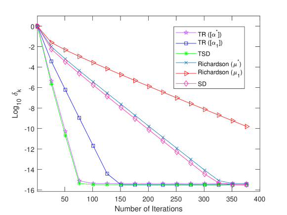
Figure 1. Convergence history of examined iterative methods for Example 3.12.

Example 3.13.

[19, Example 6.1] Let $\mathscr{A}$ in (23) be an $n\times n\times n$ tensor such that $\mathscr{A}_{::i}=A_{1}(i,1)A_{2}$ for $i=1,2\ldots,n$ in which the matrices $A_{1}$ and $A_{2}$ are respectively generated by the function $\verb|baart|(n)$ in Hansen’s package [7] and MATLAB function $\verb|gallery|(^{\prime}\verb|prolate|^{\prime},n,0.46)$.

As mentioned in [19], the coefficient tensor in the above example is severely ill-conditioned. Hence, the SD and TSD methods do not work well. Our numerical experiments also illustrate that the Richardson and TR (with $[\alpha^{*}]$) methods stagnate. However, numerical experiments show that the TR method with $[\alpha_{1}]$ can act as an iterative regularization method. To monitor the accuracy of obtained approximation corresponding to $\mathscr{X}^{*}$, the TR method (with $[\alpha_{1}]$) was used with a relative residual tolerance of $5\cdot 10^{-3}$. In this case, in average, the method stopped after about $17$ iterations and produced an approximate solution with relative error equal to $0.2601$ for $n=256$. In [19], the right-hand side tensor $\mathscr{B}$ is generated such that $\mathscr{B}=\mathscr{A}\ast\hat{\mathscr{X}}^{*}$ with $\hat{\mathscr{X}}^{*}={\rm ones}(256,1,256)$. This is a special case for which the TR method (with $[\alpha_{1}]$) requires less than five iterations with respect to our exploited stopping criterion, e.g., in a specific run it results an approximate solution with the relative error $0.0094$ after three iterations.

To improve performance of the TR method (with $[\alpha_{1}]$) for solving Example 3.13, we can combine it with some kind of relaxation step. For instance, we experimentally observed that performance of TR method (with $[\alpha_{1}]$) can be improved by using the following simple relaxation step which is originally proposed in [1] for accelerating the convergence speed of iterative methods to solve linear system of equations. To apply the relaxation step, first, let us consider the mentioned iterative methods in the following form:

$$\mathscr{X}_{k+1}=\mathscr{X}_{k}+\mathcal{F}(\mathscr{X}_{k}),\quad k=0,1,2,\ldots.$$

After performing two steps, we can add relation to the method as follows:

$$\bar{\mathscr{X}}_{k+1} = \mathscr{X}_{k}+\mathcal{F}(\mathscr{X}_{k})$$

$${\mathscr{X}}_{k+1} = {\mathscr{X}}_{k-1}+\omega_{k}(\bar{\mathscr{X}}_{k+1}-\bar{\mathscr{X}}_{k-1})$$

where, in the experimental results shown, the scalar $\omega_{k}$ is determined by minimum residual technique with respect to scalar norm of tensor at each step

$$\omega_{k}=\frac{{{{\left\langle{{\mathscr{R}_{k-1}},{\mathscr{R}_{k-1}}-{\bar{\mathscr{R}}_{k+1}}}\right\rangle}_{F}}}}{{\left\|{{\mathscr{R}_{k-1}}-\bar{{\mathscr{R}}}_{k+1}}\right\|^{2}_{F}}}$$

here $\mathscr{R}_{k-1}=\mathscr{B}-\mathscr{A}\ast\mathscr{X}_{k-1}$ and $\bar{{\mathscr{R}}}_{k+1}=\mathscr{B}-\mathscr{A}\ast\bar{{\mathscr{X}}}_{k+1}$. In Figure 2, for the sake of comparison, the performance of TR and TRR methods (with $[\alpha_{1}]$) are displayed. For TSD and SD methods, based on our observations, the above utilized relaxation step may not be successful due to the fact that the problem is too ill-conditioned. Specifically, the sequence of numerical approximation generated by TSD and SD methods even with relaxation step diverge when $n>100$ in Example 3.13. To demonstrate the effect of relaxation step, the convergence history of the methods are plotted in Figure 3 for $n=100$.

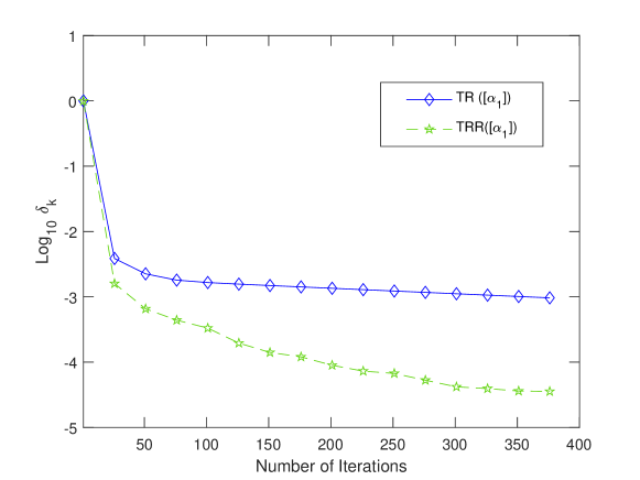
Figure 2. Convergence history of examined iterative methods in Example 3.13 for $n=256$.

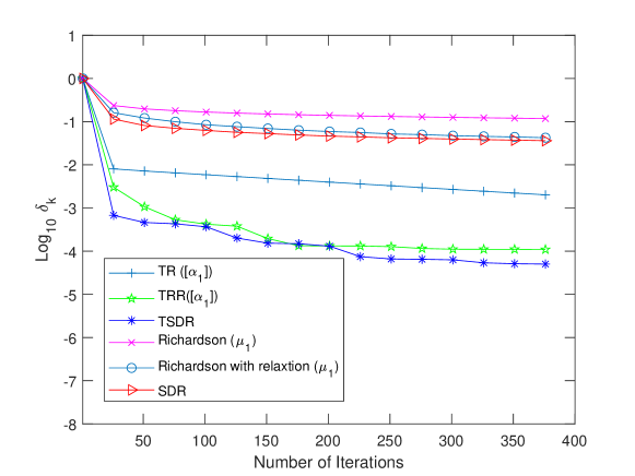
Figure 3. Convergence history of examined iterative methods in Example 3.13 for $n=100$.

4. Conclusion

We analyzed the properties of eigenvalues of third-order tensors with respect to T-product. More precisely, the eigenvalues of tensors were considered as tubular tensors. Links were established between this type of eigenvalues with T-eigenvalues and eigentuples which are two alternative definitions of eigenvalues for tensors with respect to the T-product. Some results were also included to indicate the role of tubular eigenvalues in convergence analysis of tubular iterative methods for solving tensor equation in the form $\mathscr{A}\ast\mathscr{X}=\mathscr{B}$. In addition, we briefly mentioned that the tubular form of iterative methods surpasses their alternative tensor version which is mathematically equivalent to applying them for solving ${\rm bcirc}(\mathscr{A})\textsl{Ufold}(\mathscr{X})=\textsl{Ufold}(\mathscr{B})$.

Future work that can potentially benefit from the notion of tubular eigenvalues could consider research for speeding up the convergence of tubular Krylov subspace methods to solve tensor equations with respect to T-product by proposing suitable preconditioners or using other techniques such as deflation and augmentation.

Disclosure statement

The authors declare no potential conflict of interest.

References

• [1] M. Antuono and G. Colicchio, Delayed over-relaxation for iterative methods, Journal of Computational Physics, 321 (2016), pp. 892–907.
• [2] F. P. A. Beik, A. E. Ichi, K. Jbilou, and R. Sadaka, Tensor extrapolation methods with applications, Numerical Algorithms, 87 (2021), pp. 1421–1444.
• [3] K. Braman, Third-order tensors as linear operators on a space of matrices, Linear Algebra and its Applications, 433 (2010), pp. 1241–1253.
• [4] R. H.-F. Chan and X.-Q. Jin, An introduction to iterative Toeplitz solvers, SIAM, 2007.
• [5] M. El Guide, A. El Ichi, K. Jbilou, and R. Sadaka, On tensor GMRES and Golub-Kahan methods via the T-product for color image processing, Electron. J. Linear Algebra, 37 (2021), pp. 524–543.
• [6] A. El Ichi, K. Jbilou, and R. Sadaka, On tensor tubal-Krylov subspace methods, Linear and Multilinear Algebra, (2021), pp. 1–24.
• [7] P. C. Hansen, Regularization tools version 4.0 for matlab 7.3, Numerical algorithms, 46 (2007), pp. 189–194.
• [8] N. Hao, M. E. Kilmer, K. Braman, and R. C. Hoover, Facial recognition using tensor-tensor decompositions, SIAM Journal on Imaging Sciences, 6 (2013), pp. 437–463.
• [9] H. S. Khaleel, S. V. M. Sagheer, M. Baburaj, and S. N. George, Denoising of Rician corrupted 3D magnetic resonance images using tensor-SVD, Biomedical Signal Processing and Control, 44 (2018), pp. 82–95.
• [10] M. E. Kilmer, K. Braman, N. Hao, and R. C. Hoover, Third-order tensors as operators on matrices: A theoretical and computational framework with applications in imaging, SIAM Journal on Matrix Analysis and Applications, 34 (2013), pp. 148–172.
• [11] M. E. Kilmer, L. Horesh, H. Avron, and E. Newman, Tensor-tensor algebra for optimal representation and compression of multiway data, Proceedings of the National Academy of Sciences, 118 (2021), p. e2015851118.
• [12] M. E. Kilmer and C. D. Martin, Factorization strategies for third-order tensors, Linear Algebra and its Applications, 435 (2011), pp. 641–658.
• [13] T. G. Kolda and B. W. Bader, Tensor decompositions and applications, SIAM review, 51 (2009), pp. 455–500.
• [14] W.-h. Liu and X.-q. Jin, A study on T-eigenvalues of third-order tensors, Linear Algebra and its Applications, 612 (2021), pp. 357–374.
• [15] A. Ma and D. Molitor, Randomized Kaczmarz for tensor linear systems, BIT Numerical Mathematics, 62 (2022), pp. 171–194.
• [16] Y. Miao, L. Qi, and Y. Wei, Generalized tensor function via the tensor singular value decomposition based on the T-product, Linear Algebra and its Applications, 590 (2020), pp. 258–303.
• [17]  , T-Jordan canonical form and T-drazin inverse based on the T-product, Communications on Applied Mathematics and Computation, 3 (2021), pp. 201–220.
• [18] L. Qi and X. Zhang, T-quadratic forms and spectral analysis of T-symmetric tensors, arXiv preprint arXiv:2101.10820, (2021).
• [19] L. Reichel and U. O. Ugwu, The tensor Golub–Kahan–Tikhonov method applied to the solution of ill-posed problems with a T-product structure, Numerical Linear Algebra with Applications, 29 (2022), p. e2412.
• [20]  , Tensor Arnoldi–Tikhonov and GMRES-type methods for ill-posed problems with a T-product structure, Journal of Scientific Computing, 90 (2022), pp. 1–39.
• [21]  , Weighted tensor Golub–Kahan–Tikhonov-type methods applied to image processing using a T-product, Journal of Computational and Applied Mathematics, 415 (2022), p. 114488.
• [22] Y. Saad, Iterative methods for sparse linear systems, SIAM, 2003.
• [23] C. Zeng and M. K. Ng, Decompositions of third-order tensors: HOSVD, T-SVD, and beyond, Numerical Linear Algebra with Applications, 27 (2020), p. e2290.
• [24] F. Zhang and Q. Zhang, Eigenvalue inequalities for matrix product, IEEE Transactions on Automatic Control, 51 (2006), pp. 1506–1509.