NervePool: A Simplicial Pooling Layer

Abstract

For deep learning problems on graph-structured data, pooling layers are important for down sampling, reducing computational cost, and to minimize overfitting. We define a pooling layer, NervePool, for data structured as simplicial complexes, which are generalizations of graphs that include higher-dimensional simplices beyond vertices and edges; this structure allows for greater flexibility in modeling higher-order relationships. The proposed simplicial coarsening scheme is built upon partitions of vertices, which allow us to generate hierarchical representations of simplicial complexes, collapsing information in a learned fashion. NervePool builds on the learned vertex cluster assignments and extends to coarsening of higher dimensional simplices in a deterministic fashion. While in practice, the pooling operations are computed via a series of matrix operations, the topological motivation is a set-theoretic construction based on unions of stars of simplices and the nerve complex.

1 Introduction

Design of deep learning architectures for tasks on spaces of topological objects has seen rapid development, fueled by the desire to model higher-order interactions that are naturally occurring in data. In this topological framework, we can consider data structured as simplicial complexes, generalizations of graphs that include higher-dimensional simplices beyond vertices and edges; this structure allows for greater flexibility in modeling higher-order relationships. Concepts from graph signal processing have been generalized for this higher-order network setting, leveraging operators such as Laplacian matrices [22, 20, 21]. Subsequently, there have been many developments regarding deep learning architectures that leverage simplicial (and cell) complex structure. These methods have been designed through the lens of both convolutional neural networks (CNNs) [9, 26, 6, 25, 19, 13] and message passing neural networks [5, 4]. For the purposes of this paper, we refer to neural networks within this general family as simplicial neural networks, and note that our work could be adapted and used for pooling within any of these architectures.

Typically, the pooling methods for graphs are generalizations of standard pooling layers for grids (i.e. those used in CNNs). As opposed to CNNs, which rely on a natural notion of spacial locality in the data to apply convolutions in local sections, the non-regular structure of graphs makes the spacial locality of graph pooling less obvious [27]. For this reason, many graph pooling layers for graph neural networks (GNNs) rely on local structural information represented by adjacency matrices, and coarsening operations applied directly on local graph neighborhoods. A recent survey of GNN pooling methods proposed a general framework for the operations which define different pooling layers: selection, reduction, and connection (SRC) [11]. Selection refers to the method in which vertices of the input graph are grouped into clusters; reduction computation is the aggregation of vertices into meta-vertices (and correspondingly aggregating features on vertices); connection refers to determining adjacency information of the meta-vertices and outputting the pooled graph. This broad categorization of graph pooling methods into three computational steps provides a useful framework which can be extended in a natural way to describe simplicial complex pooling.

In the simplicial complex domain, which generalizes the domain of graphs and networks, the notion of spatial locality necessary for pooling is further complicated due to the inclusion of higher-dimensional simplices. This task of coarsening simplicial complexes requires additional considerations to those of the graph coarsening task, primarily to ensure that the pooled representation upholds the definition of a simplicial complex. Naturally, simplicial complex coarsening shares some challenges with the task of coarsening graph structured data: lack of inherent spacial locality and differing input sizes (varying numbers of nodes and edges). However, the additional challenge for coarsening in the simplicial complex setting is the addition of higher dimensional simplices, with face (and coface) relations in both dimension directions by the definition of a simplicial complex. There is also a notable computational challenge when dealing with simplicial complexes due to the inherent size expansion with the addition of higher-dimensional simplices. A simplicial complex with all possible simplices included is essentially the power set of its vertices. Thus, controlling the computational explosion when using simplicial complexes in deep learning frameworks motivates the use of a pooling layer defined on the space of simplicial complexes. These pooling layers can be interleaved with regular simplicial neural network layers in order to reduce the size of the simplicial complex, which reduces computational complexity of the model and can also limit overfitting.

Existing graph pooling approaches include cluster-based methods (e.g. DiffPool [27], MinCutPool [2]) and sorting methods (e.g. TopK Pool [10, 7, 14], SAGpool [15]). There are also topologically motivated graph pooling methods such as Structural Deep Graph Mapper [3], which is based on soft cluster assignments. It uses differentiable and fixed PageRank-based lens functions for the standard Mapper algorithm [23]. Additionally, there is a method for graph pooling which uses maximal cliques [16], assigning vertices to meta-vertices using topological information encoded in the graph structure. However, if directly generalized for simplicial complexes, this clique-based coarsening method never retains any higher dimensional simplices since the pooled output is always a graph. Recently, general strategies for pooling simplicial complexes were proposed [8], which directly generalize different graph pooling methods to act on simplicial complexes: max pooling, TopK Pool [10, 7], SAGpool [15], and a TopK method separated by Hodge Laplacian terms. This proposed framework aims to generalize graph pooling methods for simplicial complexes, albeit using different tools from what we use here.

In this paper we introduce NervePool, which extends existing methods for graph pooling to be defined on the full simplicial complex using standard tools from combinatorial topology. While in practice, the pooling operations are computed via a series of matrix operations, NervePool has a compatible topological formulation which is based on unions of stars of simplices and a nerve complex construction. Like graph pooling methods, the NervePool layer for simplicial complexes can also be categorized by the SRC graph pooling framework [11], with necessary extensions for higher dimensional simplices. The main contributions of this work are as follows:

• We propose a learned coarsening method for simplicial complexes called NervePool, which can be used within neural networks defined on the space of simplicial complexes, for any standard choice of graph pooling on the vertices.

• Under the assumption of a hard partition of vertices, we prove that NervePool maintains invariance properties of pooling layers necessary for simplicial complex pooling in neural networks, as well as additional properties to maintain simplicial complex structure after pooling.

2 Background

This section gives background context for some important concepts in topological data analysis (TDA) and deep learning methods for data modeled as simplicial complexes. We first introduce relevant background on simplicial complexes, chain complexes, boundary maps between linear spaces generated by $p$-simplices, and simplicial maps. Additionally, we outline different notions of local neighborhoods on simplicial complexes through adjacency and coadjacency relations.

2.1 Simplicial Complexes

A simplicial complex is a generalization of a graph or network. While graphs can model relational information between pairs of objects (via vertices and edges connecting them), simplicial complexes are able to model higher-order interactions. With this construction, we can still model pair-wise interactions as edges, but also triple interactions as triangles, four-way interactions as tetrahedra, and so on.

The building blocks of simplicial complexes are $p$-dimensional simplices (or $p$-simplices for short), formally defined as a set of $p+1$ vertices $v_{i}\in V$,

$$\sigma_{p}=(v_{0},v_{1},\ldots,v_{p})\,,$$

where $V$ is a non-empty vertex set. Note that we often use a subscript on the simplex to denote the dimension of the simplex, i.e. $\dim(\sigma_{p})=p$. The cyclic ordering of vertex sets that constitute a simplex induce an orientation of that simplex, which can be fixed if necessary for the given task.

Simplicial complexes are collections of these $p$-simplices, glued together with the constraint that they are closed under taking subsets. In other words, an abstract simplicial complex, $K$, is a finite collection of non-empty subsets of $V$ such that for a simplex $\alpha\in K$, $\beta\subseteq\alpha$ implies $\beta\in K$. In this case we call $\beta$ a face of $\alpha$ and write $\beta\leq\alpha$. Abstract simplicial complexes are combinatorial objects, defined in terms of collections of vertices ($p$-simplices), however they have geometric realizations corresponding to vertices, edges, triangles, tetrahedra, etc. The dimension of a simplicial complex is defined as the maximum dimension of all of its simplices:

$$\dim(K)=\max_{\sigma\in K}\dim(\sigma)\,,$$

where the dimension of a simplex $\dim(\sigma)$ is one less than the cardinality of the vertex set which defines it. We denote the simplicial complex at layer $\ell$ of a neural network by $K^{(\ell)}$ and its dimension $\mathcal{P}^{(\ell)}=\dim(K^{(\ell)})$. Note that the superscript indexes the neural network layer and does not represent the $\ell$-skeleton of the complex as is common in the topology literature.

Boundary matrices and orientation

Boundary matrices provide a map between vector spaces generated by $p$-simplices and $(p-1)$-simplices. For each dimension $p$, we can define a vector space $C_{p}(K)$ with a basis given by the set of $p$-simplices and with its elements given by linear combinations of $p$-simplices. Such vector spaces are called chain groups. The boundary map $\partial_{p}$ operates on an oriented simplex $\sigma=[v_{0},\cdots,v_{p}]$ and is defined as:

$$\partial_{p}(\sigma):=\sum_{i=0}^{p}(-1)^{i}[v_{0},\cdots,\widehat{v}_{i},\cdots,v_{p}]\in C_{p-1}(K)\,,$$

where $\widehat{v}_{i}$ denotes the removal of vertex $v_{i}$ from the vertex subset. Since we are working in a linear space, this definition can be extended linearly to operate on the entire vector space $C_{p}(K)$ generated by $p$-simplices so that we have a map $\partial_{p}:C_{p}(K)\rightarrow C_{p-1}(K)$ with

$$\partial_{p}(\alpha):=\sum_{i=1}^{n_{p}}\alpha_{i}\partial_{p}(\sigma_{i})\,.$$

Each boundary matrix captures incidence relations for a given dimension, keeping track of which simplices of dimension $p-1$ are faces of a simplex of dimension $p$. For example, in Fig. 1, vertices $v_{0}$ and $v_{1}$ are on the boundary of edge $e_{0}$ and edge $e_{1}$ is on the boundary of face $f_{0}$. For each dimension $p$, this incidence-relation information is encoded in the matrices corresponding to the boundary operators $\partial_{p}$. For clarity in subsequent sections, we equivalently use notation $\partial_{p}:=\mathbf{B}_{p}\in\mathbb{R}^{n_{p-1}\times n_{p}}$ to represent the matrix boundary operator, with subscripts indicating the dimension. When necessary to associate a boundary matrix to a specific simplicial complex $K$, we denote this matrix by $\mathbf{B}_{K,p}$. Note that $\mathbf{B}_{0}=\bm{0}$, since there are no simplices of negative dimension to map down to.

Simplex orientation is encoded in boundary matrices using $\pm 1$, with different orientations of the same simplex indicated by different placement of negative values in the boundary matrix. For each simplex, there are two possible orientations, each of which are equivalence classes representing all possible cyclic permutations of the vertices which define the simplex. We say that $\sigma_{p-1}=[v_{0},v_{1},\ldots,v_{n_{p-1}}]$ and $\sigma_{p}=[w_{0},w_{1},\ldots,w_{n_{p}}]$ have the same orientation if the ordered set of vertices $[v_{0},v_{1},\ldots,v_{n_{p-1}}]$ is contained in any cyclic permutation of the vertices $w_{i}$ forming $\sigma_{p}$. Conversely, if the ordered set of vertices for $\sigma_{p-1}$ are contained in any cyclic permutations for the other orientation of $\sigma_{p}$, then we say that $\sigma_{p-1}$ and $\sigma_{p}$ have opposite orientation. Thus, we can fix an orientation and define entries of oriented $p$-boundary matrices as follows:

$$\mathbf{B}_{p}(\sigma_{p-1},\sigma_{p})=\begin{cases}1&\text{if }\sigma_{p-1}\text{ and }\sigma_{p}\text{ have the same orientation}\\ -1&\text{if }\sigma_{p-1}\text{ and }\sigma_{p}\text{ have opposite orientation}\\ 0&\text{if }\sigma_{p-1}\text{ is not a face of }\sigma_{p}\end{cases}$$

where $\sigma_{p}$ and $\sigma_{p-1}$ are simplices in $K$. If simplex orientation is not necessary, we use the non-oriented boundary matrix $\left|\mathbf{B}_{p}\right|$.

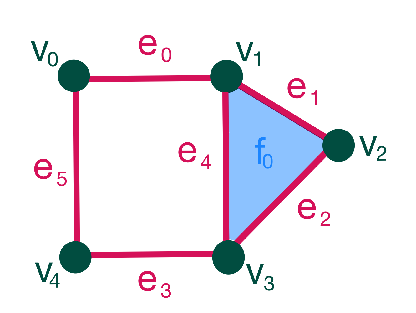
$\mathbf{B}_{1}=\blockarray{ccccccc}&{\color[rgb]{0.84765625,0.10546875,0.375}e_{0}}{\color[rgb]{0.84765625,0.10546875,0.375}e_{1}}{\color[rgb]{0.84765625,0.10546875,0.375}e_{2}}{\color[rgb]{0.84765625,0.10546875,0.375}e_{3}}{\color[rgb]{0.84765625,0.10546875,0.375}e_{4}}{\color[rgb]{0.84765625,0.10546875,0.375}e_{5}}\\ \block{c(cccccc)}{\color[rgb]{0,0.30078125,0.25}v_{0}}100001\\ {\color[rgb]{0,0.30078125,0.25}v_{1}}110010\\ {\color[rgb]{0,0.30078125,0.25}v_{2}}011000\\ {\color[rgb]{0,0.30078125,0.25}v_{3}}001110\\ {\color[rgb]{0,0.30078125,0.25}v_{4}}000101\\ \quad\mathbf{B}_{2}=\blockarray{cc}&{\color[rgb]{0.1171875,0.53515625,0.8984375}f_{0}}\\ \block{c(c)}{\color[rgb]{0.84765625,0.10546875,0.375}e_{0}}0\\ {\color[rgb]{0.84765625,0.10546875,0.375}e_{1}}1\\ {\color[rgb]{0.84765625,0.10546875,0.375}e_{2}}1\\ {\color[rgb]{0.84765625,0.10546875,0.375}e_{3}}0\\ {\color[rgb]{0.84765625,0.10546875,0.375}e_{4}}1\\ {\color[rgb]{0.84765625,0.10546875,0.375}e_{5}}0\\$

Figure 1: Non-oriented boundary matrices $\mathbf{B}_{1}$ and $\mathbf{B}_{2}$ for an example simplicial complex.

2.1.1 Simplicial Maps

A simplicial map defines a function from one simplicial complex $K_{a}$ to another $K_{b}$, specifically by a map from the vertices of $K_{a}$ to the vertices of $K_{b}$. This map $f:V(K_{a})\rightarrow V(K_{b})$ must maintain the property that all images of the vertices of a simplex span a simplex, i.e. $\forall\sigma\in K_{a},f(\sigma)\in K_{b}$ [17].

2.1.2 Adjacency

A useful way to represent a graph is by the corresponding adjacency matrix: a square matrix that stores information about which vertices are connected by edges. However, while simplicial complex structure is also captured by adjacency relations, there is more than one way to generalize this idea to higher dimensional simplices. Specifically, $p$-simplices can relate to each other by either their common upper or lower dimensional neighbors. In order to fully capture the face and coface relations in a simplicial complex, we consider four different adjacency types: boundary adjacent, coboundary adjacent, upper adjacent, and lower adjacent [5], which we define next and are shown for an example simplex in Fig. 2.

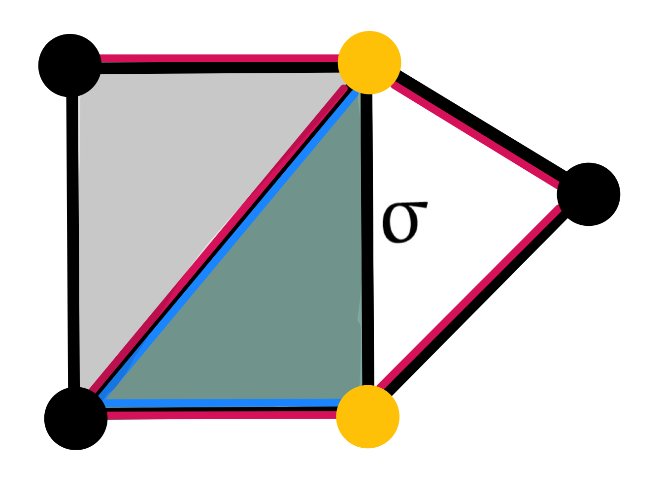
Figure 2: For simplex $\sigma$, geometrically realized as an edge, its four different types of adjacent simplices are: boundary adjacent, coboundary adjacent, lower adjacent, and upper adjacent.

Fix a $p$-simplex $\sigma_{p}$. The boundary adjacent simplices are the set of $(p-1)$-dimensional faces of the $p$-simplex. This boundary adjacent relation directly corresponds to the standard boundary map for simplicial complexes: $\mathbf{B}_{p}$. For the same simplex, the set of $(p+1)$-dimensional simplices which have $\sigma_{p}$ as a face are its coboundary adjacent simplices. The coboundary adjacency relation corresponds to the transpose of the standard boundary map: $\mathbf{B}_{p+1}^{T}$.

The usual notion of adjacency on a graph corresponds to the set of vertices which share an edge; i.e. a higher dimensional simplex with each as a face. More generally, for simplicial complexes, $p$-simplices are considered upper adjacent if there exists a $(p+1)$-simplex that they are both faces of. We can capture upper adjacent neighbor relations in terms of the complex’s boundary maps (the up-down combinatorial Laplacian operator):

(1) $$\mathbf{A}_{up,p}=\mathbf{B}_{p+1}\mathbf{B}_{p+1}^{T}\,.$$

The lower adjacent neighbors are $p$-simplices such that there exists a $(p-1)$-simplex that is a face of both (i.e. both $p$-simplices are cofaces of a common $(p-1)$-simplex). The lower adjacent neighbor relations can also be written in terms of the complex’s boundary maps (the down-up combinatorial Laplacian operator):

$$\mathbf{A}_{low,p}=\mathbf{B}_{p}^{T}\mathbf{B}_{p}\,.$$

Note that the sum of these two (upper and lower) adjacency operators gives the $p$-dimensional Hodge Laplacian, which is leveraged in different simplicial neural network architectures to facilitate local information sharing on complexes. Using the Hodge Laplacian as a diffusion operator, there are various existing neural network architectures (e.g. [5, 9]) that operate on simplicial complexes. Simplicial neural networks of this type are the context in which our pooling layer for simplicial complexes, NervePool, can be leveraged.

3 NervePool Method

In this section, we describe the proposed pooling layer defined on the space of simplicial complexes for an input simplicial complex and vertex clustering. We define both a topologically motivated framework for NervePool (Section 3.1) and the equivalent matrix representation of this method (described in Section 3.2). In Fig. 3, we visually depict both the topological and matrix formulations, and their compatible output for an example simplicial complex and vertex clustering.

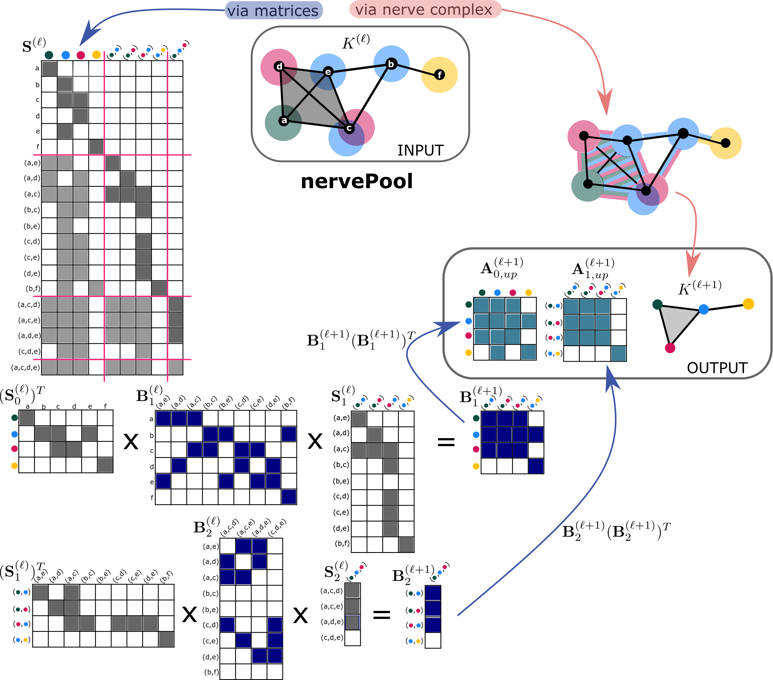
Figure 3: A visual representation of NervePool for an example simplicial complex and choice of soft partition of vertices. Shaded-in matrix entries indicate non-zero values, and elsewhere are zero-valued entries. Darker grey entry shading within the $\mathbf{S}^{(\ell)}$ matrix indicate the diagonal sub-blocks which are used for subsequent pooling operations. The output simplicial complex given by the matrix implementation is equivalent to the nerve complex output, up to weighting of $p$-simplices and the addition of “self-loops”, as indicated by non-zero entries on the diagonal of adjacency matrices.

Notation and descriptions used for simplicial complexes are outlined in Table 1.

Table 1: Simplicial complex notation and descriptions

Notation	Description
${K}^{(\ell)}$	A simplicial complex at layer $\ell$
$n_{p}^{(\ell)}$	Number of $p$-dim simplices in $K^{(\ell)}$
$\mathcal{P}^{(\ell)}$	$\text{dim}\left(K^{(\ell)}\right)$
$\mathcal{N}^{(\ell)}=\sum_{p=0}^{\mathcal{P}^{(\ell)}}n_{p}^{(\ell)}$	Total number of simplices for $K^{(\ell)}$
$d_{p}^{(\ell)}$	Number of features on $p$-dim simplices

The input to NervePool is a simplicial complex and a learned partition of the vertices (i.e. a specified cover on the vertex set). For exposition purposes, we assume that the initial clusters can form a soft partition of the vertex set, meaning every vertex is assigned to at least one cluster but vertices can have membership in more than one cluster. However, in Section 4, theoretical proof of some properties require restriction to the setting of a hard partition of the vertex set. The initial vertex clusters give us a natural way to coarsen the underlying graph ($1$-skeleton) of the input simplicial complex, where clusters of vertices in the original complex are represented by meta-vertices in the pooled complex. However, in order to collapse both structural and attributed information for higher-dimensional simplices, we require a method to extend the clusters. NervePool provides a mechanism in which to naturally extend graph pooling methods to apply on higher-dimensional simplices.

3.1 Topological Formulation

Before defining the matrix implementation of simplicial pooling, we will first describe the topological formulation using the nerve complex. NervePool follows an intuitive process built on learned vertex cluster assignments which is extended to higher dimensional simplices in a deterministic fashion.

From the input cover on just the vertex set, however, we lack cluster assignments for the higher dimensional simplices. To define a coarsening scheme on the entire complex, we must extend the cover such that each of the simplices is included in at least one cluster using a notion of local neighborhoods around each simplex. A standard way to define local neighborhoods in a simplicial complex is the star of a simplex, which can be defined on simplices of any dimension. For NervePool, we only require the star defined on vertices, $St(v)=\{\sigma_{p}\in K^{(\ell)}\mid v\subseteq\sigma_{p}\}$, which is the set of all simplices in $K^{(\ell)}$ such that $v$ is a vertex of $\sigma_{p}$. Using this construction, for each given vertex cluster $U_{i}=\{v_{0},\ldots,v_{N}\}$, we extend it to the union of the stars of all vertices in the cluster,

$$\widetilde{U}_{i}=\bigcup_{v\in U_{i}}St(v)\,.$$

The resulting cover of the complex, $\mathcal{U}=\{\widetilde{U}_{i}\}$, is such that all simplices in $K^{(\ell)}$ are part of at least (but often more than) one cover element $\widetilde{U}_{i}$. Figure 4 shows an example of a cluster consisting of three vertices and the simplices $\widetilde{U}_{i}$ which contribute to $\sigma\in K^{(\ell+1)}$.

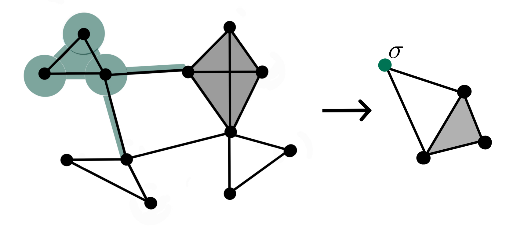
Figure 4: The three green highlighted vertices come from a single cover element $U_{i}$ of a given example cover; the full cover example will be continued in Fig. 5. The extended cover $\widetilde{U_{i}}$ for this collection of vertices, defined by the union of the star of every vertex in the cluster, is shown by the highlighted green simplices. These simplices in $K^{(\ell)}$ all contribute information to the meta vertex $\sigma\in K^{(\ell+1)}$.

Note that neither $St(v)$ nor $\widetilde{U}_{i}$ are simplicial complexes, because they are not closed under the face relation.

We use this cover of the complex to construct a new complex, using the nerve. Given any cover $\mathcal{A}=\{A_{i}\}_{i\in I}$, the nerve is defined to be the simplicial complex given by

$$\mathrm{Nrv}(\mathcal{A})=\Bigl{\{}\sigma\subseteq I\;|\;\bigcap_{i\in\sigma}A_{i}\neq\emptyset\Bigl{\}}\,,$$

where each distinct cover element $A_{i}$ is represented as a vertex in the nerve. If there is at least one simplex in two distinct cover elements $A_{i}$ and $A_{j}$, we add corresponding edge $(A_{i},A_{j})$ in the nerve complex. Similarly, for higher dimensions if there exists a $p$-way intersection of distinct cover elements, a $(p-1)$-dimensional simplex is added to the nerve complex. This general nerve construction gives us a tool to take the extended cover of the simplicial complex $\mathcal{U}=\{\widetilde{U}_{i}\}$ and define a new, pooled simplicial complex:

$$K^{(\ell+1)}:=\mathrm{Nrv}(\mathcal{U})\,.$$

Figure 5 shows the nerve of a $3$-dimensional simplicial complex using four predetermined clusters of the vertices.

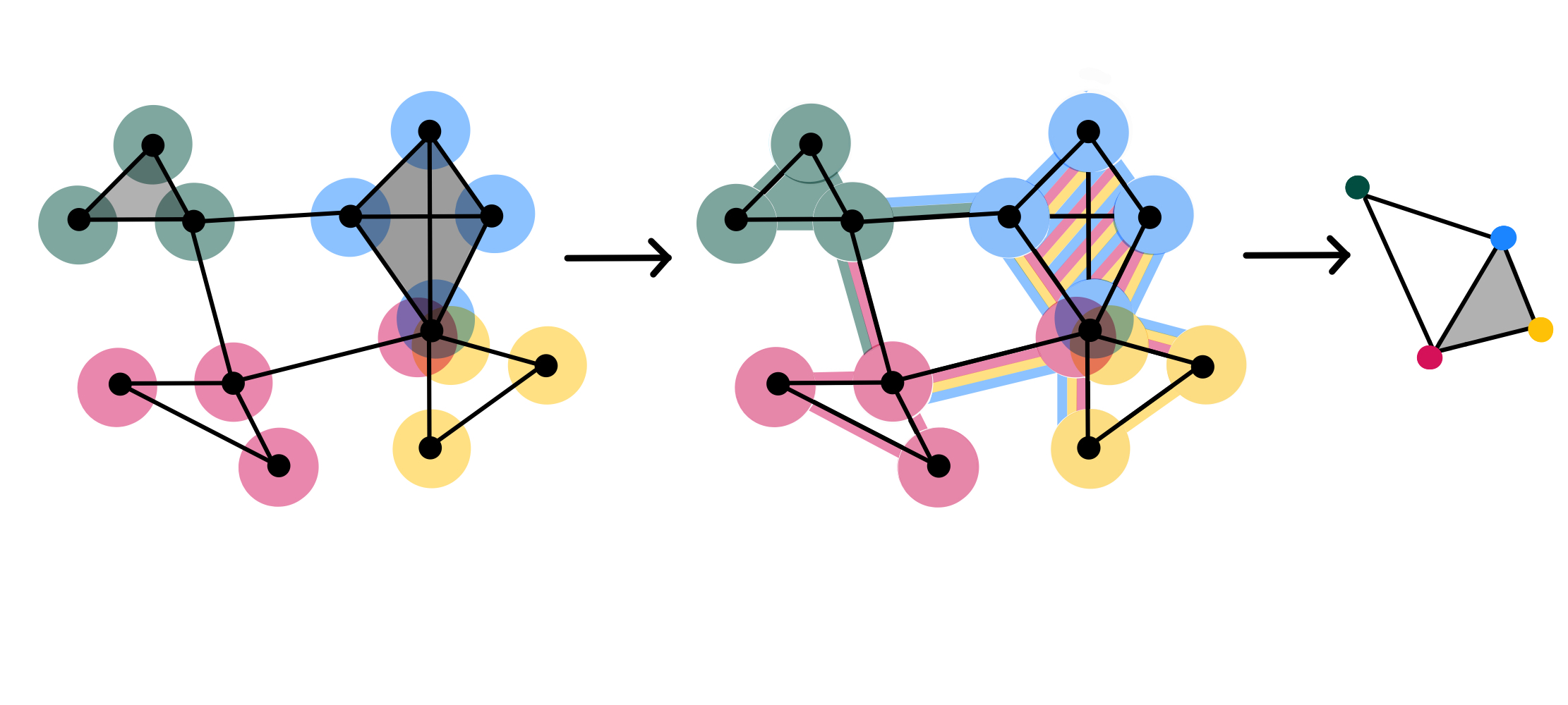
Figure 5: Illustration NervePool on an example $3$-dim simplicial complex, applied to coarsen the complex into a $2$-dimensional simplicial complex. The left-most complex is the input simplicial complex, with vertex cluster membership indicated by color. The center complex depicts the extended clusters $\mathcal{U}=\{\widetilde{U}_{i}\}$ and the right-most complex is the pooled simplicial complex, determined by $Nrv(\mathcal{U})$.

A notable feature of the extended covers that facilitate NervePool is that they are based on the learned vertex cluster assignments and as such, cover elements are not necessarily contractible. Vertex clusters that are spatially separated on the complex can result in cover elements that are non-convex. Thus, since open cover elements are not guaranteed to be convex, we cannot guarantee that the simplicial complex $K^{(\ell+1)}=\mathrm{Nrv}(\mathcal{U})$ is homotopy-equivalent to the original complex $K^{(\ell)}$ as would be needed to apply the nerve lemma [24].

3.2 Matrix Implementation

In practice, we apply the simplicial pooling method described above through matrix operations on constructed cluster assignment matrices, boundary matrices, and simplex feature matrices. Matrix notation used to define simplicial pooling is outlined in Table 2. See also Table 1 for simplicial complex notation.

Table 2: Matrix notation with dimensions

Notation	Dimension	Purpose
$\mathbf{A}_{p}^{(\ell)}$	$n_{p}^{(\ell)}\times n_{p}^{(\ell)}$	Adjacency matrix for $p$-dim simplices at layer $\ell$
$\mathbf{B}_{p}^{(\ell)}$	$n_{p-1}^{(\ell)}\times n_{p}^{(\ell)}$	$p$-dimensional boundary matrix. Maps features on $p$-dim simplices to the space of $(p-1)$-dim simplices
$\mathbf{X}_{p}^{(\ell)}$	$n_{p}^{(\ell)}\times d_{p}^{(\ell)}$	Features on $p$-dim simplices at layer $\ell$
$\mathbf{S}^{(\ell)}$	$\mathcal{N}^{(\ell)}\times\mathcal{N}^{(\ell+1)}$	Block matrix for pooling simplices at layer $\ell$
$\mathbf{S}_{q,p}^{(\ell)}$	$n_{q}^{(\ell)}\times n_{p}^{(\ell+1)}$	Sub-block of $\mathbf{S}^{(\ell)}$ matrix which maps $q$-simplices in $K^{(\ell)}$ to $p$-simplices in the pooled complex $K^{(\ell+1)}$. If $q=p$, we write $\mathbf{S}_{q}^{(\ell)}$

For this paper, we assume that the input boundary matrices that represent each simplicial complex are non-oriented, meaning the matrix values are all non-negative. Since the nerve complex is an inherently non-oriented object (built using intersections of sets of simplices) and NervePool is formulated based on a nerve construction, it is necessary that the boundary matrices we use to represent each simplicial complex similarly do not take orientation into account; we use $\left|\mathbf{B}_{p}\right|$ for NervePool pooling operations. However, if the other layers of the neural network that the pooling layer is used within require orientation of simplices, it is sufficient to fix an arbitrary orientation (so long as it is consistent between dimensions of the complex). For example, using an orientation equivariant message passing simplicial neural network (MPSN) layer, we can fix an orientation of simplices after applying NervePool without affecting full network invariance with respect to orientation transformations [5].

Extend vertex cluster assignments

From the input vertex cover, we represent cluster membership of each $0$-simplex (vertex) in an assignment matrix $\mathbf{S}_{0}^{(\ell)}$. This $n_{0}^{(\ell)}\times n_{0}^{(\ell+1)}$ matrix keeps track of the vertex clusters with entries $\mathbf{S}_{0}^{(\ell)}[\sigma_{0}^{(\ell)},U_{i}]>0$ if the vertex $\sigma_{0}^{(\ell)}$ is in cluster $U_{i}$ and zero entries elsewhere. Each row of $\mathbf{S}_{0}^{(\ell)}$ corresponds to a vertex in the original complex, and each column corresponds to a cover element (or cluster), represented as a meta-vertex in the next layer $\ell+1$. Using these initial clusters which consist of vertices only, we then extend the cluster assignments to include all of the higher dimensional simplices of the complex in a deterministic way. From the original matrix $\mathbf{S}_{0}^{(\ell)}:n_{0}^{(\ell)}\times n_{0}^{(\ell+1)}$, we extend the pooling to all simplices resulting in the full matrix, $\mathbf{S}^{(\ell)}:\mathcal{N}^{(\ell)}\times\mathcal{N}^{(\ell+1)},$ where each of its sub-blocks $\mathbf{S}_{q,p}^{(\ell)}:n_{q}^{(\ell)}\times n_{p}^{(\ell+1)}$ map $q$-simplices in $K^{(\ell)}$ to $p$-simplices in the coarsened complex $K^{(\ell+1)}$. Figure 6 shows a visualization of this matrix extension from vertex cluster assignments to all dimension simplex cluster assignments.

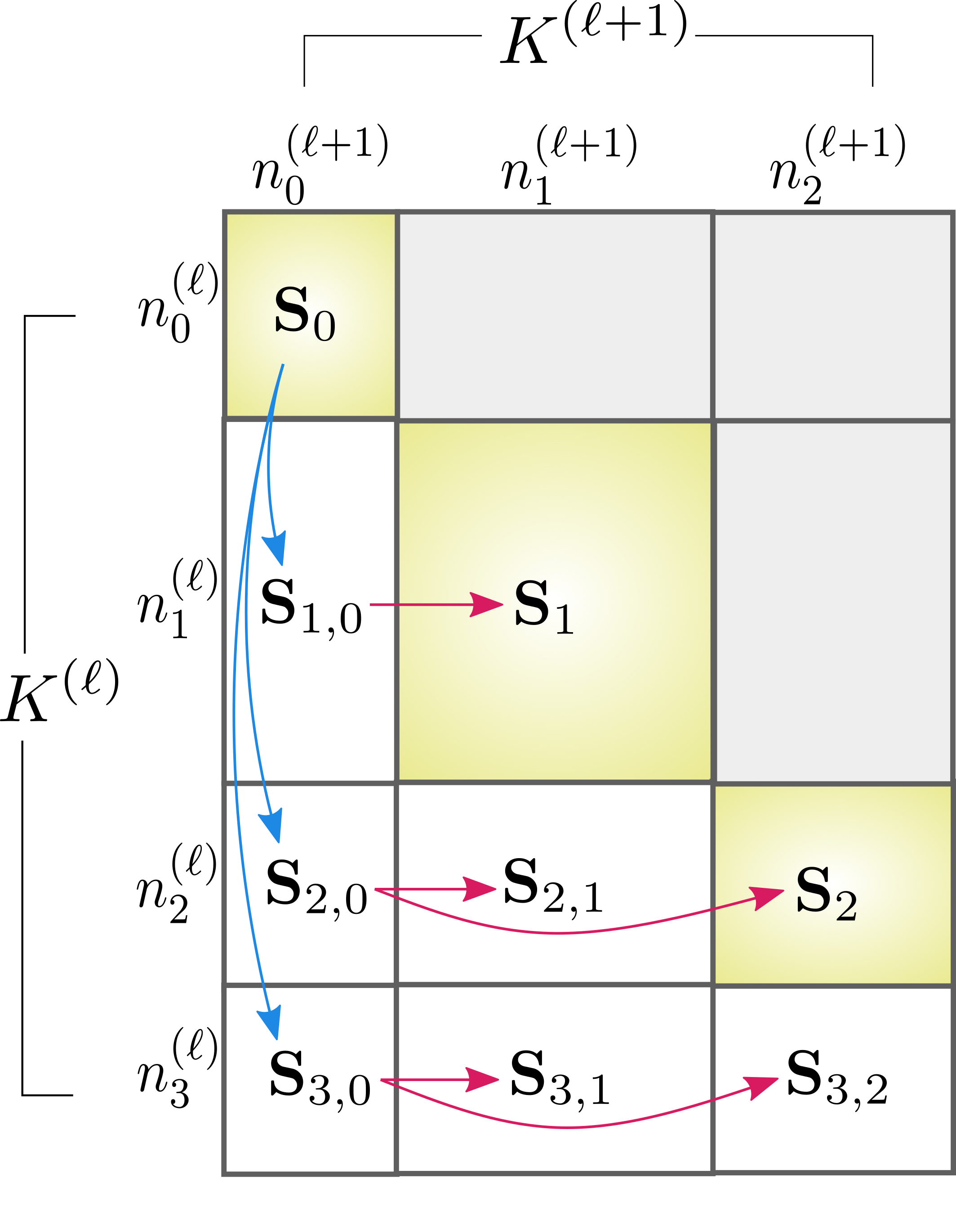
Figure 6: Visual depiction of $\mathbf{S}^{(\ell)}:\mathcal{N}^{(\ell)}\times\mathcal{N}^{(\ell+1)}$ block matrix. Sets of sub-blocks are used to map simplices of original simplicial complex to the pooled simplices. Diagonal sub-blocks (highlighted in yellow) are used directly for pooling.

As visualized in this diagram, there are two directions by which information is cascaded through the matrix $\mathbf{S}^{(\ell)}$: extend down and extend right, both of which pass information to simplices of the next higher dimension. Only the diagonal sub-blocks of $\mathbf{S}^{(\ell)}$ are used to pool simplices downstream, so we limit the information cascading to the down and right updates, and ignore possible upper triangular entries. We pass pooling information to simplices of the next higher dimension, within the original simplicial complex via the down arrow update, $\mathbf{S}_{0}{\color[rgb]{0.1171875,0.53515625,0.8984375}\rightsquigarrow}\,\mathbf{S}_{q,0},$ for $q>0$ defined,

(2) $$\mathbf{S}_{q,0}[\sigma_{q},v_{j}]:=\begin{cases}1&\text{if }\mathbf{S}_{0}[v_{m},v_{j}]=1\text{ for any }v_{m}\in\sigma_{q}\\ 0&\text{ otherwise.}\end{cases}$$

Pooling information is passed to simplices of higher dimensions for the new simplicial complex via the right arrow update, $\mathbf{S}_{q,0}{\color[rgb]{0.84765625,0.10546875,0.375}\rightsquigarrow}\,\mathbf{S}_{q,p}$, for $0<p\leq q$

(3) $$\mathbf{S}_{q,p}[\cdot,\sigma_{p}]:=\mathbf{S}_{q,0}[\cdot,v_{a}]\odot\mathbf{S}_{q,0}[\cdot,v_{b}]\odot\cdots\odot\mathbf{S}_{q,0}[\cdot,v_{c}]\,,$$

for $\sigma_{p}$ the simplex given by $(v_{a},v_{b},\ldots,v_{c})$ and where $\odot$ indicates the pointwise multiplication of matrix columns. If $\mathbf{S}_{q,p}[\cdot,\sigma_{p}]=\bm{0}$ (the zero vector) then $\sigma_{p}\notin K^{(\ell+1)}$ and that column is not included in $\mathbf{S}_{q,p}$.

Cluster assignment normalization

Cluster assignments for all of the $p$-simplices should be probabilistic, since the underling partition of the vertices are learned cluster assignments. For example, if the vertex clustering method used follows that of DiffPool on the underlying graph, the cluster assignment matrix is given by a softmax applied to GNN output. In this scenario, the input cluster assignment matrix contains probabilistic assignments of each vertex to one or more clusters. To achieve this normalization across all dimensions of the complex, we row-normalize the lower triangular matrix $\mathbf{S}^{(\ell)}$. The result of this normalization is that for a given $p$-simplex in $K^{(\ell)}$, the total contributions to pooled $q$-simplices in $K^{(\ell+1)}$ sum to $1$, where $q\leq p$, i.e. each row of the lower-triangular assignment matrix $\mathbf{S}^{(\ell)}$ sums to $1$.

Pool with full cluster assignment matrix

Only the diagonal sub-blocks of $\mathbf{S}^{(\ell)}$ are directly used to pool simplices of a complex $K^{(\ell)}$ to the pooled complex $K^{(\ell+1)}$. Sub-blocks of the pooling matrix correspond to mapping $p$-dimensional simplices in $K^{(\ell)}$ to pooled $p$-simplices in $K^{(\ell+1)}$. In particular, the $p$-dimensional boundary matrices of the pooled simplicial complex are computed using

$$\mathbf{B}_{p}^{(\ell+1)}=\left(\mathbf{S}_{p-1}^{(\ell)}\right)^{T}\mathbf{B}_{p}^{(\ell)}\mathbf{S}_{p}^{(\ell)}.$$

Then, the pooled simplicial complex is entirely determined by the upper adjacency matrices (Equation 1), $\mathbf{A}_{up,p}^{(\ell+1)}=\mathbf{B}_{p+1}^{(\ell+1)}\left(\mathbf{B}_{p+1}^{(\ell+1)}\right)^{T}$, either on their own or normalized using the absolute difference with the degree matrix $\mathbf{D}_{p}=\sum_{j=0}^{n_{p}}B_{p+1}$,

$$\mathbf{A}_{up,p}^{(\ell+1)}=\left|\,\mathbf{D}_{p}-\mathbf{B}_{p+1}^{(\ell+1)}\left(\mathbf{B}_{p+1}^{(\ell+1)}\right)^{T}\right|\,.$$

The set of pooled boundary matrices, or alternatively the set of upper adjacency matrices, give all of the structural information necessary to define a simplicial complex. Note that the specific adjacency representation is a choice, and one could use alternative notions of adjacency described in Section 2.1 to summarize the pooled simplicial complex. Simplex embeddings are also aggregated according to the cluster assignments in $\mathbf{S}^{(\ell)}$ to generate coarsened feature matrices for simplices in layer $\ell+1$. We compute these pooled embeddings for features on $p$-simplices by setting

(4) $$\mathbf{X}_{p}^{(\ell+1)}=(\mathbf{S}_{p}^{(\ell)})^{T}\mathbf{X}_{p}^{(\ell)}\,,$$

where $\mathbf{X}_{p}^{(\ell)}$ are the features on $p$-simplices. The coarsened boundary matrices and coarsened feature matrices for each dimension can then be used as input to subsequent layers in the network.

The matrix implementation of NervePool, using cluster assignment matrices multiplied against boundary matrices, is consistent with the set-theoretical topological nerve construction outlined in Section 3.1. Given the same complex and initial vertex cover, the output pooled complex using the nerve construction is structurally equivalent to the simplicial complex described by $\mathbf{A}_{up,p}^{(\ell+1)}$. Refer to Theorem 4.1 and associated proof for a formal description of this equivalence.

3.3 Note on differentiability

For training of a simplicial neural network, and specifically to apply NervePool layers, the computations defining NervePool need not be continuous and differentiable. Gradients are not defined on the higher-order simplices of each complex, only on the underlying graph. So, to use gradient descent and perform backpropagation for network training, the simplicial complex is simply recomputed after the learned vertex pooling stage using the NervePool method. Equations 2 and 3 facilitate this deterministic computation of coarsening for the higher dimensional simplices.

3.4 Training NervePool

The required input to NervePool is a partition of the vertices of a simplicial complex, learned using only the $1$-skeleton (underlying graph) of the complex. Since the learned aspect of NervePool is limited to the vertex cluster assignments ($\mathbf{S}_{0}^{(\ell)}$) and higher-dimensional cluster assignments are a deterministic function of $\mathbf{S}_{0}^{(\ell)}$, the loss functions used for cluster assignments are defined on only vertices and edges of the complex. Any trainable graph pooling method that learns a soft partition of the graph (DiffPool [27], MinCutPool [2], StructPool [28], etc) can be used in conjunction with NervePool. However, there are minor adjustments necessary to modify these graph pooling methods for application to NervePool simplicial complex coarsening (primarily in terms of computing embeddings for multiple dimensions).

The broad categorization of graph pooling methods into selection, reduction, and connection (SRC) computations [11] provide a useful framework to classify steps of NervePool and necessary extensions for the higher dimensional simplices. The selection step refers to the method for grouping vertices of the input graph into clusters, which can be used directly in the case of NervePool on the $1$-skeleton for the initial vertex covers. The reduction computation, which aggregates vertices into meta-vertices (and correspondingly features on vertices aggregated), must be generalized and computed for every dimension of the simplicial complex. In the case of NervePool, this is done using the diagonal sub-blocks of $\mathbf{S}^{(\ell)}$ to perform the reduce step at each dimension. Similarly, the connect step requires generalization to higher dimensions and computation of new boundary maps to output the pooled simplicial complex. Table 3 summarizes trainable graph pooling methods, modified for use within NervePool simplicial complex pooling as the learned-vertex clustering input method.

Table 3: Trainable Graph Pooling Methods in the SRC framework, with necessary adjustments for higher-dimensional use within NervePool. MLP is a multi-layer perceptron defined on the vertex features, $\beta$ a regularization vector, and $\mathbf{i}$ a vector of indices. Table adapted from [11].

Graph Pooling	Select	Reduce ($\forall\,p$)	Connect ($\forall\,p$)
MinCutPool [2]	$\mathbf{S}_{0}^{(\ell)}=MLP(\mathbf{X}_{0}^{(\ell)})$	$\mathbf{X}_{p}^{(\ell+1)}=(\mathbf{S}_{p}^{(\ell)})^{T}\mathbf{X}_{p}^{(\ell)}$	$B_{p}^{(\ell+1)}=(\mathbf{S}_{p-1}^{(\ell)})^{T}\mathbf{B}_{p}\mathbf{S}_{p}$
NFM [1]	Factorize: $\mathbf{A}_{0}^{(\ell)}=\mathbf{W}\mathbf{H}\rightarrow\mathbf{S}_{0}^{(\ell)}=\mathbf{H}^{T}$	$\mathbf{X}_{p}^{(\ell+1)}=(\mathbf{S}_{p}^{(\ell)})^{T}\mathbf{X}_{p}^{(\ell)}$	$B_{p}^{(\ell+1)}=(\mathbf{S}_{p-1}^{(\ell)})^{T}\mathbf{B}_{p}\mathbf{S}_{p}$
LaPool [18]	$\begin{cases}\mathbf{V}=\lVert\mathbf{L_{0}}\mathbf{X}_{0}\rVert_{d}\\ \mathbf{i}=\{i|\forall j\in\mathcal{N}(i):\mathbf{V}_{i}\geq\mathbf{V}_{j}\}\\ \mathbf{S}_{0}^{(\ell)}=\text{SparseMax}\left(\beta\frac{\mathbf{x}_{0}\mathbf{x}_{0,i}^{T}}{\lVert\mathbf{x}_{0}\rVert\lVert\mathbf{x}_{0},i\rVert}\right)\end{cases}$	$\mathbf{X}_{p}^{(\ell+1)}=(\mathbf{S}_{p}^{(\ell)})^{T}\mathbf{X}_{p}^{(\ell)}$	$B_{p}^{(\ell+1)}=(\mathbf{S}_{p-1}^{(\ell)})^{T}\mathbf{B}_{p}\mathbf{S}_{p}$

NervePool extended using DiffPool graph pooling

For DiffPool [27] graph pooling, the vertex clusters are learned using a GNN, so for the simplicial complex extension, $\mathbf{S}_{0}^{(\ell)}$ can be learned with an MPSN layer [5]. Using diagonal block matrices of the extended matrix $\mathbf{S}^{(\ell)}$, the reduce step is applied for every dimension of the complex. Finally, the connections of the pooled complex are determined by multiplying cluster assignment matrices against boundary matrices, for each dimension of the complex. NervePool (specifically using DiffPool for vertex cluster assignments) is summarized in Table 4 in terms of the necessary select, reduce, and connect steps.

Table 4: DiffPool adjustment for NervePool in the SRC [11] framework.

Select	$\mathbf{S}_{0}^{(\ell)}=softmax[MPSN_{\ell,pool}(\mathbf{B}_{1}^{(\ell)},\mathbf{X}_{0}^{(\ell)},\mathbf{X}_{1}^{(\ell)})]$
Reduce ($\forall p$)	$\mathbf{X}_{p}^{(\ell+1)}=(\mathbf{S}_{p}^{(\ell)})^{T}\cdot MPSN_{\ell,embed}(\mathbf{B}_{p}^{(\ell)},\mathbf{B}_{p+1}^{(\ell)},\mathbf{X}_{p-1}^{(\ell)},\mathbf{X}_{p}^{(\ell)},\mathbf{X}_{p+1}^{(\ell)})$
Connect ($\forall p$)	$\mathbf{B}_{p}^{(\ell+1)}=(\mathbf{S}_{p-1}^{(\ell)})^{T}\mathbf{B}_{p}\mathbf{S}_{p}$

Additionally, Fig. 7 shows an overview flowchart of NervePool, as implemented via matrices, when the choice of vertex clusters is based on DiffPool-style graph pooling. To extend DiffPool on graphs to simplicial complex coarsening, we must use separate MPSNs to pool features on simplices for each dimension and an additional MPSN to find a soft partition of vertices. These separate message passing networks (embedding MPSNs and the pooling MPSN) require distinct learnable parameter matrices $\Theta_{p,embed}^{(\ell)}$ and $\Theta_{pool}^{(\ell)}$.

For each pooling layer, a collection of embedding MPSNs take as input the features on simplices (for the current dimension $\mathbf{X}_{p}^{(\ell)}$, a dimension lower $\mathbf{X}_{p-1}^{(\ell)}$, and a dimension higher $\mathbf{X}_{p+1}^{(\ell)}$) and boundary matrices (for the current dimension $\mathbf{B}_{p}^{(\ell)}$ and one dimension higher $\mathbf{B}_{p+1}^{(\ell)}$). The output of which is an embedding matrix $\mathbf{Z}_{p}^{(\ell)}\in\mathbb{R}^{n_{p}^{(\ell)}\times d_{p}^{(\ell)}}$ for every dim $0\leq p\leq\mathcal{P}^{(\ell)}$ of the complex $K^{(\ell)}$. Here, $n_{p}^{(\ell)}$ is the number of $p$-simplices at layer $\ell$, and $d_{p}^{(\ell)}$ is the number of $p$-simplex features. These matrices are the learned $p$-simplex embeddings defined by

$$\mathbf{Z}_{p}^{(\ell)}=MPSN_{\ell,embed}(\mathbf{B}_{p}^{(\ell)},\mathbf{B}_{p+1}^{(\ell)}\mathbf{X}_{p-1}^{(\ell)},\mathbf{X}_{p}^{(\ell)},\mathbf{X}_{p+1}^{(\ell)};\Theta_{p,embed}^{(\ell)})\,,$$

where $\Theta_{p,embed}^{(\ell)}$ is the matrix of learnable weights at layer $\ell$. Note that for the pooling MPSN, which is restricted to dimension $p=0$, the message passing reduces to a function

$$MPSN_{\ell,pool}(\mathbf{B}_{1}^{(\ell)},\mathbf{X}_{0}^{(\ell)},\mathbf{X}_{1}^{(\ell)})\,.$$

The second component of NervePool, illustrated by the right-side branch in Fig. 7, determines the pooling structure through cluster assignments for each simplex. For an input simplicial complex, $K^{(\ell)}$, with features on $p$-simplices, $\{\mathbf{X}_{p}^{(\ell)}\}_{p=0}^{\mathcal{P}^{(\ell)}}$, we use an MPSN on the underlying graph of the simplicial complex. In the same fashion as the DiffPool method for graph pooling (Equation $5$ in [27]), we generate an assignment matrix for vertices (vertex cover) via

$$\mathbf{S}_{0}^{(\ell)}=softmax\left[MPSN_{\ell,pool}(\mathbf{B}_{1}^{(\ell)},\mathbf{X}_{0}^{(\ell)},\mathbf{X}_{1}^{(\ell)};\Theta_{pool}^{(\ell)})\right]\,,$$

where the output $\mathbf{S}_{0}^{(\ell)}\in\mathbb{R}^{n_{0}^{(\ell)}\times n_{0}^{(\ell+1)}}$ is the learned vertex cluster assignment matrix at layer $\ell$. Note that the MPSN for dimension $p=0$ acting on the $1$-skeleton of $K^{(\ell)}$, reduces to a standard GNN. Learning the pooling assignment matrix requires only this single MPSN, for dimension $p=0$ simplices. From this single pooling MPSN, $\mathbf{S}_{0}^{(\ell)}$ gives a soft assignment of each vertex at layer $\ell$ to a cluster of vertices in the next coarsened layer $\ell+1$.

In terms of network training, the DiffPool learning scheme for $\mathbf{S}_{0}^{(\ell)}$ uses two additional loss terms added to the normal supervised loss for the entire complex. These loss terms are added from each NervePool layer to the simplicial complex classification loss during training of the entire network to encourage local pooling of the simplicial complex and to limit overlapping cluster assignments. The first term is a link prediction loss, which encourages clustering of vertices which are spatially nearby on the simplicial complex,

$$\mathcal{L}_{LP}=||\mathbf{A}_{0}^{(\ell)},\,\mathbf{S}_{0}^{(\ell)}(\mathbf{S}_{0}^{(\ell)})^{T}||_{F}\,,$$

where $||\cdot||_{F}$ denotes the Frobenius norm. The second term is a cross entropy loss, which is used to limit the number of different clusters a single vertex can be assigned to, given by

$$\mathcal{L}_{E}=\frac{1}{n_{0}^{(\ell)}}\sum_{i=1}^{n_{0}^{(\ell)}}H(\mathbf{S}_{0}^{(\ell)}(i,\cdot))\,,$$

where $H$ is the entropy function and $\mathbf{S}_{0}^{(\ell)}(i,\cdot)$ the $i$-th row of the vertex cluster assignment matrix at layer $\ell$. Both of the additional loss terms $\mathcal{L}_{LP}$ and $\mathcal{L}_{E}$ are minimized and for each NervePool layer, added to the total simplicial complex classification loss at the end of the network. Training a NervePool layer reduces to learning a soft partition of vertices of a graph, since the extension to coarsening of higher-dimensional simplices are deterministic functions of the vertex clusters.

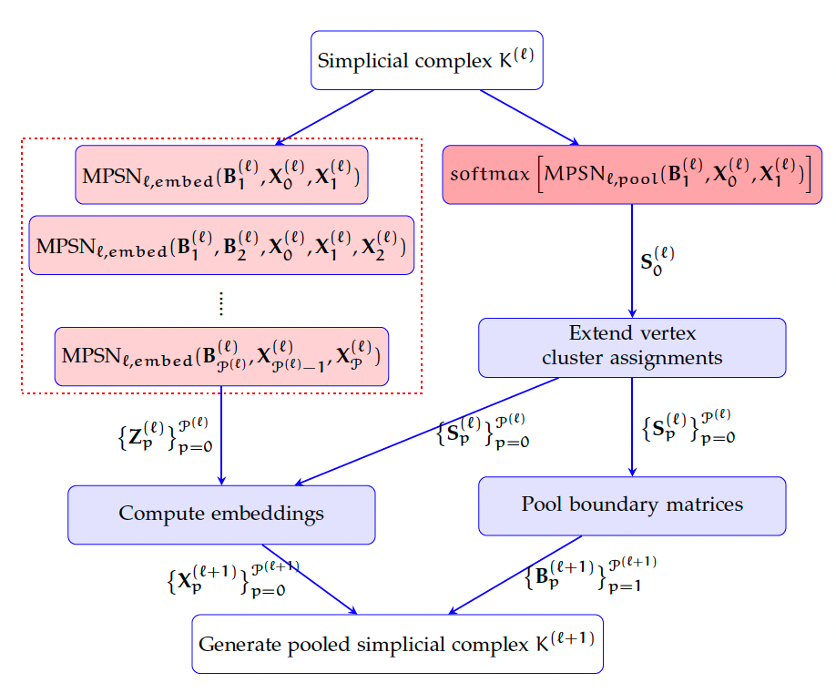
Figure 7: Example NervePool architecture, using DiffPool as the motivating vertex cluster method. Takes input simplicial complex $K^{(\ell)}$ and returns the pooled simplicial complex $K^{(\ell+1)}$. The left-side branch uses a collection of MPSNs to compute embeddings for each dimension (Reduce step). The right-side branch illustrates using an MPSN to compute vertex cluster assignments (Select step), and then extending assignments to higher dimensional simplices so that this structural information facilitates collapsing of simplices when applied against boundary matrices (Connect step).

4 NervePool Properties

In this section, we describe observational and theoretical properties of NervePool as a learned simplicial complex coarsening method, including a formally defined identity function. In practice, most learned graph pooling methods output soft partitions of the vertex set, meaning a vertex can be included in multiple clusters. However, extraneous non-zero entries in the “boundary” matrices built by NervePool emerge from vertices assigned to multiple clusters. While the result is a matrix that does not in fact represent a simplicial complex, they do not seem to pose an issue in practice, so long as the output simplicial complex is represented by its adjacency matrices, and not the “boundary” matrices. The unintended entries of “boundary” matrices do not affect the adjacency matrix representation because if one is present in the matrix, then there must also be non-zero entries present for the edges that appear in the adjacency matrix.

As a result, in practice NervePool can be used in a hard- or soft-partition setting. However to prove equivalence of the nerve construction to the matrix implementation and simplex-permutation invariance, we must assume a hard vertex clustering, i.e. where each vertex is a member of exactly one cluster. In this regime, NervePool has more theoretical justification and we can derive the matrix implementation in a way such that it produces the same pooled simplicial complex output as the nerve construction, provided they are given the same input complex and vertex cover. Additionally, assuming a hard partition of the vertex set allows us to prove it is a simplex permutation invariant pooling layer. To work in this more restricted setting, given a soft-partition input, one could simply threshold appropriately to ensure that each vertex is assigned to a single cluster, choosing the cluster it is included in with the highest probability. See the example of Fig. 8 for the resulting matrices in the case of a hard partition, which uses the same complex as the soft partition example of Fig. 3. In this restricted case, the boundary matrix output of NervePool does not have any extra non-zero entries that we see in the case of soft partitions on the vertex set.

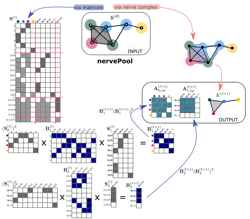
Figure 8: A visual representation of NervePool for an example simplicial complex and choice of vertex clusters. Note this is the same simplicial complex as Fig. 3, but using a hard partition of the vertex set. Matrix entries indicate non-zero values, and elsewhere are zero-valued entries. Darker grey entry shading within the $\mathbf{S}^{(\ell)}$ matrix indicate the diagonal sub-blocks which are used for subsequent pooling operations.

We note one technical distinction between the standard graph representation as an adjacency matrix, and the generalized adjacency matrices we use here. In the standard literature, the diagonal of the adjacency matrix of a graph will be zero unless self loops are allowed. However, the adjacency matrices constructed here have a slightly different viewpoint. In particular (at least in the hard partition setting), an entry of an upper-adjacency matrix for dimension $p$ simplices is non-zero if the two simplices share a common higher dimensional coface. In the case of a graph, the $0$-dimensional upper-adjacency matrix would then have non-zero entries on the diagonal since a vertex that is adjacent to any edge is thus upper adjacent to itself.

Another important technical note is that with no assumptions on the input clustering, we cannot make promises about maintaining the topological structure of the simplicial complex heading into the pooled layer. Since the vertex cluster assignments are largely task-dependent, any collection of vertices can be grouped together in a cluster if it minimizes the loss function with respect to a given task, with no regard for their spatial locality on the simplicial complex. This can lead to potentially un-intuitive behaviour in the simplex pooling for those used to working in the setting of the nerve lemma [24], specifically learned vertex groupings which are not localized clusters. For example, Fig. 9 shows three different initial vertex covers of same input simplicial complex, resulting in three different NervePool outcomes of simplicial complexes with different homology.

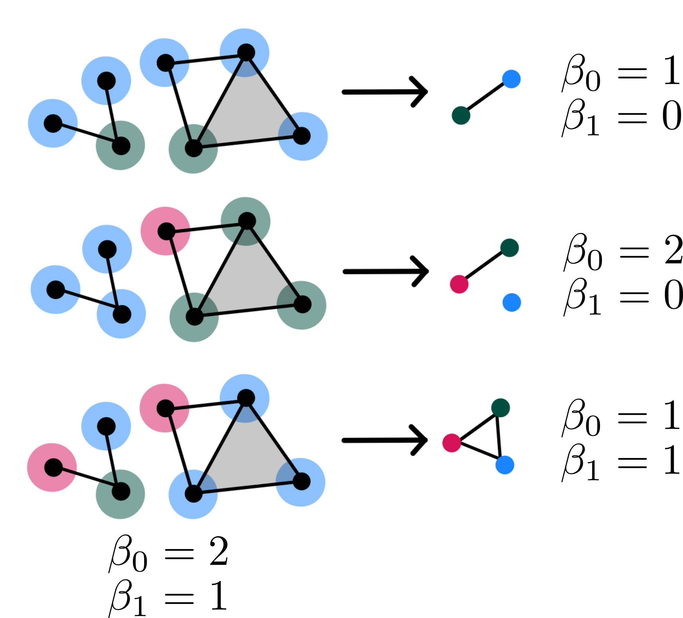
Figure 9: An input simplicial complex with three different choices of initial vertex covers (top, middle, bottom). Each of these cover choices produce pooled simplicial complexes of different homology using NervePool, as indicated by the Betti numbers for dimensions $0$ and $1$. The first initial vertex cover (top) produces NervePool output which changes Betti numbers in both dimensions. The second cover (middle) produces an output complex with the same $0$-dim Betti number. The third cover (bottom) produces an output complex with the same $1$-dim Betti number.

In addition to interpretability of the diagonal entries, the hard partition assumption gives further credence for connecting the topological nerve/cover viewpoint with the matrix implementation presented. We prove this connection in the next theorem, which hinges on the following construction. Assume we are given the input cover of the vertex set $\{U_{i}\}_{i=1}^{n_{0}^{(\ell+1)}}$, have constructed the cover of the simplicial complex using the stars of the vertices $\mathcal{U}=\{\widetilde{U}_{i}\}_{i=1}^{n_{0}^{(\ell+1)}}$ and have built the pooled simplicial complex using the nerve construction $K^{(\ell+1)}=\mathrm{Nrv}(\mathcal{U})$. There is a natural simplicial map $f:K^{(\ell)}\to K^{(\ell+1)}$ where a vertex $v\in K^{(\ell)}$ is mapped to the vertex in $K^{(\ell+1)}$ representing the (unique due to the hard partition assumption) cover element containing it. As with any simplicial map, simplices in $K^{(\ell)}$ may be mapped to simplices in $K^{(\ell+1)}$ of a strictly lower dimension. Our assumption of using only the block diagonal of the $\mathbf{S}^{(\ell)}$ matrix means that the matrix construction version will essentially ignore these lower dimensional maps, instead focusing on the portions of the simplicial map that maintain dimension. That being said, one could make some different choices in the pipeline to maintain these simplices with the trade-off of additional computation time required.

Theorem 4.1 (Equivalence of Topological and Matrix Formulations).

Given the same input simplicial complex and hard partition of the vertex set (cluster assignments), the topological nerve/cover viewpoint and matrix implementation of NervePool produce the same pooled simplicial complex.

Proof 4.2.

The proof that these two methods result in the same simplicial complex is broken into two parts:

1. The maps are the same. We will show that the matrix representation $\mathbf{M}$ of the natural simplicial map $f:K^{(\ell)}\rightarrow\mathrm{Nrv}(\mathcal{U})=K^{(\ell+1)}$ discussed above, is equal to the matrix $\mathbf{S}^{(\ell)}$ of simplex cluster assignments used for pooling in the matrix formulation.

2. The complexes (boundary matrices) are the same. The boundary matrices which represent the nerve of the cover $\mathcal{U}$ are equal to the boundary matrices computed using the boundary and cluster assignment matrices from layer $\ell$. That is, we will show

   $$\mathbf{B}_{\mathrm{Nrv}(\mathcal{U}),p}=\left(\mathbf{S}_{p-1}^{(\ell)}\right)^{T}\mathbf{B}_{p}^{(\ell)}\mathbf{S}_{p}^{(\ell)}$$

   and thus represent the same complex which we can denote as $K^{(\ell+1)}$.

Proof of (i): We prove equivalence of the simplicial map $f:K^{(\ell)}\rightarrow K^{(\ell+1)}$ to the matrix $\mathbf{S}^{(\ell)}$ of simplex cluster assignments by showing equivalent sparsity patterns of their matrices. The simplicial map is defined as $f(\sigma)=\{f(v)\}_{v\in\sigma}$, removing duplicates where they occur and viewing the result as a simplex in $K^{(\ell+1)}$. Writing $U_{v}$ for the (unique because of the hard cover assumption) cluster containing vertex $v$ (and noting that there could be different representatives), let $\{U_{v_{0}},\cdots,U_{v_{p}}\}$. Let $\mathbf{M}$ be the matrix that represents this operator, so by definition, $\mathbf{M}[\sigma,\tau]\geq 1$ iff $\tau\leq f(\sigma)$, i.e. if $\tau$ is a face of $f(\sigma)$. By the nerve construction, for cover elements $U_{v_{i}}$ representing vertices of $\tau$, $\bigcap_{i=0}^{p}\widetilde{U}_{v_{i}}\neq\emptyset$.

By definition of Eqns. 2 and 3, to fill in entries of the $\mathbf{S}^{(\ell)}$ matrix, an entry $\mathbf{S}[\sigma,\tau]$ is nonempty iff $\mathbf{S}[\sigma,U_{v}]\neq 0$ for all $U_{v}\in\tau$. By definition, this means that $\sigma$ has at least one vertex in each of the cover elements $U_{v}$, and thus $\sigma\in\bigcap\widetilde{U}_{v_{i}}$. From the previous discussion, this happens iff $M[\sigma,\tau]\geq 1$.
Proof of (ii): Assume we are given a pair $\tau_{p-1}\leq\tau_{p}$ simplices in $\mathrm{Nrv}(\mathcal{U})$, so that

$$\mathbf{B}_{Nrv(\mathcal{U}),p}[\tau_{p-1},\tau_{p}]\neq 0.$$

We will first show that if this occurs, the matrix multiplication results in a nonzero entry $\mathbf{B}_{p}^{(\ell+1)}[\tau_{p-1},\tau_{p}]\neq 0$ as well. If $\{U_{v_{0}},\cdots,U_{v_{p}}\}$ are the cover elements representing vertices of $\tau_{p}$, we know that there exists a $\sigma\in\bigcap_{i=0}^{p}\widetilde{U}_{v_{i}}$. By the star construction, this implies that every $U_{v_{i}}$ must contain at least one vertex of $\sigma$, and because of the hard cluster assumption, we then have $\dim(\sigma)\geq\dim(\tau_{p})=p$. Let $\sigma_{p}\leq\sigma$ be a face of $\sigma$ with exactly one vertex per cover element, and note that $\sigma_{p}\in\bigcap_{i=0}^{p}\widetilde{U}_{v_{i}}$ as well. Finally, writing $\tau_{p-1}=\{U_{v_{0}},\cdots,\widehat{U}_{v_{i}},\cdots,U_{v_{p}}\}$, let $\sigma_{p-1}\leq\sigma_{p}$ be the face which does not have a vertex in $U_{v_{i}}$. As we have assumed non-negative entries in all matrices and because there exist non-zero entries in $\mathbf{S}_{p-1}^{(\ell)T}[\tau_{p-1},\sigma_{p-1}]$, $\mathbf{B}_{p}^{(\ell)}[\sigma_{p-1},\sigma_{p}]$, and $\mathbf{S}_{p}^{(\ell)}[\sigma_{p},\tau_{p}]$, the resulting matrix multiplication

$$\mathbf{B}_{p}^{(\ell+1)}=\left(\mathbf{S}_{p-1}^{(\ell)}\right)^{T}\mathbf{B}_{p}^{(\ell)}\mathbf{S}_{p}^{(\ell)}$$

will also have a non-zero entry in $[\tau_{p-1},\tau_{p}]$.

Conversely, if the pair $\tau_{p-1}$ is not a face of $\tau_{p}$, there is at least one vertex $U_{v_{1}}$ in $\tau_{p-1}$ which is not in $\tau_{p}$, and using the dimension difference, there are at least two vertices $U_{v_{2}},U_{v_{3}}$ which are in $\tau_{p}$ but not $\tau_{p-1}$. Given any $\sigma_{p}\in K^{(\ell)}$, we will show that at least one of $\mathbf{S}_{p-1}^{(\ell)T}[\tau_{p-1},\sigma_{p}]$, and $\mathbf{S}_{p}^{(\ell)}[\sigma_{p},\tau_{p}]$ are zero, resulting in a zero entry in the matrix multiplication. If $\mathbf{S}_{p}^{(\ell)}[\sigma_{p},\tau_{p}]=0$ we are done, so assume this entry is not zero. By definition, this means that $f(\tau_{p})=\sigma_{p}$. Following the same argument above, this means that $\sigma_{p}$ has a vertex in each cover element $U_{v}$ of $\tau_{p}$. Given any $\sigma_{p-1}\leq\sigma_{p}$, there is exactly one vertex $U_{v}$ missing. However, either $U_{v_{2}}$ or $U_{v_{3}}$ must still be included in $\sigma_{p-1}$. These were found because they are not in $\tau_{p-1}$, thus $f(\sigma_{p-1})\neq\tau_{p-1}$. As the $\mathbf{S}^{(\ell)}$ matrix represents the simplicial map $f$, we then have that $\mathbf{S}_{p-1}^{(\ell)T}[\tau_{p-1},\sigma_{p-1}]=0$ as required.

Theorem 4.3 (NervePool identity function).

There exists a choice of cover (cluster assignments) on the vertices, $\mathbf{S}_{0}^{(\ell)}$, such that NervePool is the identity function, i.e. $K^{(\ell+1)}=K^{(\ell)}$ and the pooled complex is equivalent to the original, up to re-weighting of simplices. In particular, this choice of $\mathbf{S}_{0}^{(\ell)}$ mapping is such that each distinct vertex in $K^{(\ell)}$ is assigned to a distinct vertex cluster in $K^{(\ell+1)}$.

Proof 4.4.

For the proof, we show a bijection between the simplicial complexes using the set-theoretic representations, thus showing that the resulting layer is the same up to reweighting of the simplicies. Suppose each vertex in the original complex is assigned to a distinct cluster, so that $U_{i}=\{v_{i}\}$, and then $\widetilde{U_{i}}=\mathrm{St}(v_{i})$. For any simplex $\sigma=\{v_{i_{0}},\cdots,v_{i_{d}}\}$ in $K^{(\ell)}$, we denote $\widetilde{\sigma}=\{\widetilde{U_{i_{0}}},\cdots,\widetilde{U_{i_{d}}}\}$. Note that $\widetilde{\sigma}$ must be a simplex in $K^{(\ell+1)}$ since $\sigma$ is in the intersection of the stars $\bigcap_{i=i_{0}}^{i_{d}}\mathrm{St}(v_{i})$.

Injectivity is immediate by definition. We show the bijectivity of the set map $K^{(\ell)}\to K^{(\ell+1)}$ sending $\sigma\mapsto\widetilde{\sigma}$. To check surjectivity, note that for any $\widetilde{\sigma}\in K^{(\ell+1)}$ with $\{\widetilde{U_{i_{0}}},\cdots,\widetilde{U_{i_{d}}}\}$, the intersection $\bigcap_{i=i_{0}}^{i_{d}}\mathrm{St}(v_{i})$ must contain some simplex $\tau$. By definition, this means that $v_{i}\leq\tau$ for all $i\in\{i_{0},\cdots i_{d}\}$. Then $\sigma=\{v_{i_{0}},\cdots,v_{i_{d}}\}\leq\tau$, and by the closure of the simplicial complex, $\sigma\in K^{(\ell)}$.

Permutation invariance

A key property of graph structured data and graph neural networks is that the re-ordering of vertices should not affect the network output. Different representations of graphs by their adjacency information are equivalent, up to arbitrary reordering of the vertices. This property implies a permutation invariant network is necessary for most tasks such as graph classification, and subsequently permutation invariant pooling layers are necessary. Other types of invariance, including orientation of simplices, are not relevant for NervePool, due to the assumption of non-oriented simplices.

Theorem 4.5 (NervePool Permutation Invariance).

NervePool is a permutation invariant function on the input simplicial complex and partition of vertices. Equivalently,

$$\text{{{NervePool}}{}}(P\mathbf{S}_{0}^{(\ell)},K^{(\ell)})=\text{{{NervePool}}{}}(\mathbf{S}_{0}^{(\ell)},K^{(\ell)})\,,$$

for any permutation matrix on vertices $P\in\{0,1\}^{n_{0}^{(\ell)}\times n_{0}^{(\ell)}}$.

Proof 4.6.

Permutations of simplices correspond to re-ordering of the vertex list of a complex. Note that the re-ordering of vertices of a simplicial complex induces a corresponding re-ordering of all its higher dimensional simplices. Consider a simplicial complex defined by its set of simplicies $K:=\{\sigma_{0},\ldots,\sigma_{n}\}$. Consider an alternate labeling of all simplices in $K$ and call this new simplicial complex $K^{\prime}:=\{\sigma_{0}^{\prime},\ldots,\sigma_{n}^{\prime}\}$. Then, there exists an isomorphism between the sets $K$ and $K^{\prime}$, and specifically an isomorphism between the vertex sets of each. This map between vertices in $K$ and vertices in $K^{\prime}$ can be represented by a permutation matrix $P\in\{0,1\}^{n_{0}^{(\ell)}\times n_{0}^{(\ell)}}$. Then, $\text{{{NervePool}}{}}(P\mathbf{S}_{0}^{(\ell)},K^{(\ell)})=\text{{{NervePool}}{}}(\mathbf{S}_{0}^{(\ell)},K^{(\ell)})$ since the simplex sets define the same simplicial complex structure and the vertex cluster assignments are permuted accordingly.

5 Code and implementation notes

NervePool code is available at www.github.com/sarah-mcguire/nervePool. The implementation takes an input simplicial complex (given by either a list of simplices or set of boundary matrices) and partition of vertices (array assignment matrix $\mathbf{S}_{0}^{(\ell)}$) and returns the pooled simplicial complex. There is also built-in functionality to visualize each simplicial complex using NetworkX [12]. In the case of hard clusters of the vertex set for pooling, the complex visualization can also include highlights around each vertex, with color indicating each vertex’s cluster membership. The current implementation of NervePool is limited to input simplicial complexes with maximum dimension 3 (where the largest simplices are tetrahedra). Additionally, vertices are labeled and tracked using ASCII characters, so the maximum number of vertices which a simplicial complex can have is $128$ in the current version.

6 Conclusions and Future Directions

In this paper, we have defined a method to extend learned graph pooling methods to simplicial complexes. Given a learned partition of vertices, NervePool returns a coarsened and simplified simplicial complex, where simplices and signals defined on those simplices are redistributed on the output complex. This framework for simplicial complex coarsening is a very flexible method because the input partition of the vertex set can come from any choice of standard graph pooling method or learned vertex clustering. We show that there is a choice of input cover on the vertices such that NervePool returns the same simplicial complex (up to re-weighting) and that when used in the context of a simplicial neural network with hard vertex clusters, it is a simplex-permutation invariant layer. Additionally, we prove the equivalence of the nerve/cover topological interpretation and matrix implementation using boundary matrices for the setting restricted to hard vertex partitions. This pooling layer has potential applications in a range of deep learning tasks such as classification and link prediction, in settings where the input data can be naturally modeled as a simplicial complex. NervePool can help to mitigate the additional computation cost of including higher dimensional simplices when using simplicial neural networks: reducing complex dimension, while redistributing information defined on the simplicial complex in a way that is optimized for the given learning task.

A limitation of this method is that using standard graph pooling methods for the initial clustering of vertices limits the learned influence of higher-dimensional simplices. Future work in this direction to include more topological information in the learning of vertex clusters could enhance the utility of this method for topologically motivated tasks. For graph pooling methods with auxiliary loss terms such as DiffPool [27] and MinCutPool [2], adjustment or inclusion of additional auxiliary topological loss terms to encourage vertex clusters with topological meaning would be an interesting line of inquiry. Taking into account the higher-dimensional structure for the learned pooling on underlying graphs could allow NervePool to coarsen simplicial complexes, tuned such that specified topological structure is retained from the original complex.

While the current assumptions of NervePool include loss functions only defined on the $1$-skeleton, if additional auxiliary loss terms defined on higher-order simplices were utilized, then the functions defining NervePool would need to be continuous and differentiable for gradient computations. This is automatic for Equation 3, the right arrow update, since it defines a series of Hadamard (entry-wise) products, which are differentiable. However, Equation 2 is an “on or off” function, which is not differentiable. To address this, one could define a relaxation of the update rule which closely approximates the rule with a differentiable function (e.g. sharp sigmoidal or capped Relu-type functions). Such considerations for gradient computation could be addressed in future work, adjusting loss function choices to preserve desired topological structure in the pooled representation of simplicial complexes.

In this paper, to compute embeddings of features on $p$-simplices $\{\mathbf{X}_{p}^{(\ell+1)}\}_{p=0}^{\mathcal{P}^{(\ell+1)}}$, we choose to apply separate coarsening for each dimension of the input simplicial complex in Equation 4. This choice enforces that information sharing for the signals defined on simplices only affect signals on pooled simplices within a given dimension. Alternatively, future modifications could utilize the entire block matrix $\mathbf{S}^{(\ell)}$ applied against a matrix containing signals on simplices of all dimensions, which would allow for signal information to contribute to pooled simplices amongst different dimensions.

Additional future work on simplicial complex coarsening should include experimental results to identify cases where including simplicial pooling layers improve, for example, classification accuracy. Also, comparison experiments at different layers of a simplicial neural network would be useful to determine if the pooled complexes are reasonable and/or meaningful representations of the original simplicial complexes, with respect to a given task.

References

- [1] D. Bacciu and L. D. Sotto, A non-negative factorization approach to node pooling in graph convolutional neural networks, CoRR, abs/1909.03287 (2019), http://arxiv.org/abs/1909.03287, https://arxiv.org/abs/1909.03287.
- [2] F. M. Bianchi, D. Grattarola, and C. Alippi, Spectral clustering with graph neural networks for graph pooling, in International Conference on Machine Learning, PMLR, 2020, pp. 874–883.
- [3] C. Bodnar, C. Cangea, and P. Liò, Deep graph mapper: Seeing graphs through the neural lens, Frontiers in big Data, 4 (2021).
- [4] C. Bodnar, F. Frasca, N. Otter, Y. Wang, P. Lio, G. F. Montufar, and M. Bronstein, Weisfeiler and Lehman go cellular: Cw networks, Advances in Neural Information Processing Systems, 34 (2021), pp. 2625–2640.
- [5] C. Bodnar, F. Frasca, Y. Wang, N. Otter, G. F. Montufar, P. Lio, and M. Bronstein, Weisfeiler and Lehman go topological: Message passing simplicial networks, in International Conference on Machine Learning, PMLR, 2021, pp. 1026–1037.
- [6] E. Bunch, Q. You, G. Fung, and V. Singh, Simplicial 2-complex convolutional neural networks, in TDA & Beyond, 2020, https://openreview.net/forum?id=TLbnsKrt6J-.
- [7] C. Cangea, P. Veličković, N. Jovanović, T. Kipf, and P. Liò, Towards sparse hierarchical graph classifiers, arXiv preprint arXiv:1811.01287, (2018).
- [8] D. M. Cinque, C. Battiloro, and P. Di Lorenzo, Pooling strategies for simplicial convolutional networks, 2022, https://doi.org/10.48550/ARXIV.2210.05490.
- [9] S. Ebli, M. Defferrard, and G. Spreemann, Simplicial neural networks, 2020, https://arxiv.org/abs/2010.03633.
- [10] H. Gao and S. Ji, Graph u-nets, in international conference on machine learning, PMLR, 2019, pp. 2083–2092.
- [11] D. Grattarola, D. Zambon, F. M. Bianchi, and C. Alippi, Understanding pooling in graph neural networks, CoRR, abs/2110.05292 (2021), https://arxiv.org/abs/2110.05292, https://arxiv.org/abs/2110.05292.
- [12] A. A. Hagberg, D. A. Schult, and P. J. Swart, Exploring network structure, dynamics, and function using networkx, in Proceedings of the 7th Python in Science Conference, G. Varoquaux, T. Vaught, and J. Millman, eds., Pasadena, CA USA, 2008, pp. 11 – 15.
- [13] A. D. Keros, V. Nanda, and K. Subr, Dist2cycle: A simplicial neural network for homology localization, Proceedings of the AAAI Conference on Artificial Intelligence, 36 (2022), pp. 7133–7142, https://doi.org/10.1609/aaai.v36i7.20673.
- [14] B. Knyazev, G. W. Taylor, and M. Amer, Understanding attention and generalization in graph neural networks, Advances in neural information processing systems, 32 (2019).
- [15] J. Lee, I. Lee, and J. Kang, Self-attention graph pooling, in International conference on machine learning, PMLR, 2019, pp. 3734–3743.
- [16] E. Luzhnica, B. Day, and P. Lio, Clique pooling for graph classification, arXiv preprint arXiv:1904.00374, (2019).
- [17] J. R. Munkres, Elements of algebraic topology, CRC press, 1984.
- [18] E. Noutahi, D. Beaini, J. Horwood, and P. Tossou, Towards interpretable sparse graph representation learning with laplacian pooling, CoRR, abs/1905.11577 (2019), http://arxiv.org/abs/1905.11577, https://arxiv.org/abs/1905.11577.
- [19] T. M. Roddenberry, N. Glaze, and S. Segarra, Principled simplicial neural networks for trajectory prediction, in Proceedings of the 38th International Conference on Machine Learning, M. Meila and T. Zhang, eds., vol. 139 of Proceedings of Machine Learning Research, PMLR, 18–24 Jul 2021, pp. 9020–9029, https://proceedings.mlr.press/v139/roddenberry21a.html.
- [20] T. M. Roddenberry, M. T. Schaub, and M. Hajij, Signal processing on cell complexes, CoRR, abs/2110.05614 (2021), https://arxiv.org/abs/2110.05614, https://arxiv.org/abs/2110.05614.
- [21] S. Sardellitti and S. Barbarossa, Topological signal representation and processing over cell complexes, 2022, https://arxiv.org/abs/2201.08993.
- [22] M. T. Schaub, Y. Zhu, J.-B. Seby, T. M. Roddenberry, and S. Segarra, Signal processing on higher-order networks: Livin’ on the edge… and beyond, Signal Processing, 187 (2021), p. 108149, https://doi.org/https://doi.org/10.1016/j.sigpro.2021.108149.
- [23] G. Singh, F. Mémoli, and G. E. Carlsson, Topological methods for the analysis of high dimensional data sets and 3d object recognition., PBG@ Eurographics, 2 (2007).
- [24] A. Weil, Sur les théoremes de de rham, Comment. Math. Helv, 26 (1952), pp. 119–145.
- [25] M. Yang and E. Isufi, Convolutional learning on simplicial complexes, 2023, https://doi.org/10.48550/ARXIV.2301.11163, https://arxiv.org/abs/2301.11163.
- [26] M. Yang, E. Isufi, and G. Leus, Simplicial convolutional neural networks, CoRR, abs/2110.02585 (2021), https://arxiv.org/abs/2110.02585, https://arxiv.org/abs/2110.02585.
- [27] Z. Ying, J. You, C. Morris, X. Ren, W. Hamilton, and J. Leskovec, Hierarchical graph representation learning with differentiable pooling, Advances in neural information processing systems, 31 (2018).
- [28] H. Yuan and S. Ji, Structpool: Structured graph pooling via conditional random fields, in International Conference on Learning Representations, 2020, https://openreview.net/forum?id=BJxg_hVtwH.