From Lindblad master equations to Langevin dynamics and back

Abstract

A case study of the non-equilibrium dynamics of open quantum systems in the markovian approximation is presented for two dynamical models based on a single harmonic oscillator in an external field. Specified through distinct forms of ohmic damping, their quantum Langevin equations are derived from an identical set of physical criteria, namely the canonical commutator between position and momentum, the Kubo formula, the virial theorem and the quantum equilibrium variance. The associated Lindblad equations are derived but only one of them is completely positive. Transforming those into Fokker-Planck equations for the Wigner functions, both models are shown to evolve towards the same Gibbs state, for a vanishing external field. The phenomenological differences between the models are illustrated through their quantum relaxations and through the phase diagrammes derived from their re-interpretation as mean-field approximations of an interacting many-body system.

I Introduction

The description of the non-equilibrium dynamics of open quantum systems continues to present many challenges Breuer and Petruccione (2002); Cugliandolo (2003); Gardiner and Zoller (2004); Schaller (2014); Täuber (2014); Breuer et al. (2016); De Vega and Alonso (2017); Weiss (2022). In spite of much progress, many details of the modelling of the interaction of the degrees of freedom of the system and the bath(s) are far from obvious. In the celebrated system-interaction-bath framework, exact quantum Langevin equations can be derived. From these microscopic derivations, the quantum fluctuation-dissipation theorem (qfdt) follows, such that the relaxation towards the thermodynamic equilibrium state is guaranteed, but the resulting dynamics cannot be markovian Ford et al. (1965, 1988); Gardiner and Zoller (2004); Hänggi and Ingold (2005); Sieberer et al. (2015); Ford (2017); Araújo et al. (2019); Weiss (2022). Here, we are interested in physical situations with a large separation of the time-scales between the system and the bath such that an effective and approximate markovian description of the system’s dynamics becomes feasible.

Effective markovian dynamics are often specified in terms of dynamic semi-groups. When expressed as a master equation for the reduced density matrix $\hat{\rho}$ with the degrees of freedom of the bath integrated out, its Liouvillian generator can be shown to reduce to a Lindblad form Lindblad (1976a). Explicit justifications of the Lindblad equations are usually based on second-order perturbation theory and product initial states which are uncorrelated between the ‘system’ and the ‘bath’. Under these conditions, it can be shown that mixtures must be preserved under the dynamics from which it follows that the Lindblad dissipators should be completely positive Lindblad (1976a); Alicki and Lendi (2007); F. Benatti (2001); Alicki (1995); Pechukas (1995); Sargolzahi (2022). However, the validity of these hypothesis, notably the tensor product form of the initial states, has been questioned Pechukas (1994); Alicki (1995); Pechukas (1995); Romero et al. (2004); Shaji and Sudarshan (2005); Carteret et al. (2008); Rodríguez-Rosario et al. (2008); Dominy and Lidar (2016) and it is claimed that complete positivity is not really required as a dynamic postulate. Recent approaches try to circumvent this controversial question Becker et al. (2022); Correia et al. (2021); Vallejos et al. (2022); Colla et al. (2022). A different view is that all this would be an artefact of an ill-defined evolution map Schmid et al. (2019).

On the other hand, in Langevin equations the coupling between the system and the bath(s) is described in terms of deterministic damping terms and importantly through stochastic noise terms whose correlators must be specified in order to render the required physical behaviour, notably the requested properties of the stationary state Zwanzig (2001); de Oliveira (2020); Weiss (2022). For reduced open quantum systems with effective markovian dynamics, both the lindbladian and langevinian descriptions co-exist but there is hardly any discussion on their mutual relationship.

The quantum harmonic oscillator has served since a long time as paradigm, also for quantum dynamics, e.g. Lindblad (1976b); Bedeaux and Mazur (2001); Bedeaux (2002); Carmichael (1999); Breuer and Petruccione (2002); Gardiner and Zoller (2004); de Oliveira (2020); Weiss (2022) and refs. therein. The Lindblad description is usually based on the quantum optics situation of a single oscillator in a cavity which does provide explicit expressions for the dissipator, e.g. Carmichael (1999); Breuer and Petruccione (2002); Gardiner and Zoller (2004) and which is manifestly completely positive. For a Langevin description, the physical starting point will be a massive particle in a harmonic potential and submitted to a frictional force. We shall use here the form proposed by Bedeaux and Mazur Bedeaux and Mazur (2001); Bedeaux (2002) which was obtained from a master equation of the reduced density matrix $\hat{\rho}$. We intend to use this paradigm to analyse possible relationships between these two formulations of effective markovian dynamics of open quantum systems, in the form of a case study. We shall regard both formulations as a means to obtain equations of motion for averaged observables and regard two descriptions as equivalent if they lead to the same equations of motion (up to canonical transformations). The markovian nature of the effective Langevin dynamics is described here through noise correlators which depends on the two times $t,t^{\prime}$ only through delta functions $\delta(t-t^{\prime})$. By itself, this means that such a form can only hold true after some short transient time $\tau_{\rm micro}$ such that any peaked ‘initial’ noise correlator will converge to a delta-correlated form for times $t,t^{\prime}$ or $t-t^{\prime}\gg\tau_{\rm micro}$, with a microscopic reference time $\tau_{\rm micro}$.

Specifically, our programme will be as follows. In section II, we recall the Bedeaux-Mazur formulation of the markovian quantum Langevin equation (to be called friction model) and also define the cavity model as a quantum harmonic oscillator with different deterministic damping terms. Both models are special cases of a more general system studied long ago Lindblad (1976b). In both models, the explicit noise correlators will be determined from the same set of phenomenological requirements (A-D) which we formulate. In any case, whatever more microscopic justification might be found in either model, these must lead to certain phenomenological consequences so that we can impose these ‘physically reasonable’ consequences immediately. In this way, not only we can avoid any explicit discussion of complete positivity, but via the explicit formulations available we can proceed to a discussion of the relaxational behaviour, rather than having to rely on rather abstract mathematically-inspired systems usually discussed in the litterature. Since we use the same physical criteria to define both models, it is clear that they share the same physical foundation. The exact solutions of the Langevin equations of both models are given and are seen to be in-equivalent, not least since the friction model contains an ‘over-damped’ dynamical regime which is absent in the cavity model. In section III, we recall first that the cavity model is equivalent to the standard Lindbladian description of a harmonic oscillator in a cavity Carmichael (1999); Breuer and Petruccione (2002); Gardiner and Zoller (2004) and hence manifestly completely positive Alicki and Lendi (2007). We then construct the master equation of the reduced density matrix of the friction model which turns out to be positive, but not completely positive. Rather, its dissipator is the difference of two completely positive dissipators, which is the most general form mathematically possible for a positive matrix Ando (2018). Comparing the dynamic behaviour of the two models therefore allows to have a simple physical illustration on the effects of positivity, compared to complete positivity, of the density matrix. This illustration will be brought in section IV where the master equations of both models are solved simultaneously via the Wigner function technique. Again this illustrates that both models share the same mathematical basis, although they are physically distinct. While both models relax to the same equilibrium distribution (at least in the case without an external field) their dynamics if different. In section V we recast both models as mean-field approximations of a many-body interacting magnet and analyse the nature of their respective relaxations and phase diagrams at zero temperature. While the friction model relaxes to an equilibrium state independent of the damping parameter $\gamma$, the cavity model produces a non-trivial re-entrant phase diagram and its $\gamma$-dependent stationary state cannot reach equilibrium. Our conclusions are given in section VI. Several appendices contain technical details and background.

II Quantum Langevin equations

Our study concerns a single harmonic oscillator, with Hamiltonian

$$\hat{H}=\frac{g}{2}\hat{p}^{2}+\frac{\omega^{2}}{2g}\hat{x}^{2}-B\hat{x}=\hbar\omega\bigg{(}\hat{a}^{\dagger}\hat{a}+\frac{1}{2}\bigg{)}-B\sqrt{\frac{\hbar g}{2\omega}\,}\,(\hat{a}+\hat{a}^{\dagger})$$ (II.1)

where $g$ is the quantum coupling, $\omega$ is the angular frequency and and $\hat{x},\hat{p}$ are the position and momentum operators which obey the commutation relation $\commutator{\hat{x}}{\hat{p}}={\rm i}\hbar$ and can be re-expressed through bosonic creation and annihilation operators

$$\hat{x}=\sqrt{\frac{\hbar g}{2\omega}\,}\,\bigl{(}\hat{a}^{{\dagger}}+\hat{a}\bigr{)}\;\;,\;\;\hat{p}={\rm i}\sqrt{\frac{\hbar\omega}{2g}\,}\,\bigl{(}\hat{a}^{\dagger}-\hat{a}\bigr{)}$$ (II.2)

which leads to the second form of $\hat{H}$ in (II.1). In application to quantum magnets, where $\hat{s}=\hat{x}$ becomes a quantum spin variable, $B$ is interpreted as an external magnetic field. We shall compare the dynamics generated by the Langevin equations, namely the friction model with

$$\partial_{t}\hat{x}=\frac{{\rm i}}{\hbar}\commutator{\hat{H}}{\hat{x}}+\hat{\eta}^{(x)}\;\;,\;\;\partial_{t}\hat{p}=\frac{{\rm i}}{\hbar}\commutator{\hat{H}}{\hat{p}}-\gamma\hat{p}+\hat{\eta}^{(p)}$$ (II.3a)

and the cavity model where

$$\partial_{t}\hat{x}=\frac{{\rm i}}{\hbar}\commutator{\hat{H}}{\hat{x}}-\frac{\gamma}{2}\hat{x}+\hat{\eta}^{(x)}\;\;,\;\;\partial_{t}\hat{p}=\frac{{\rm i}}{\hbar}\commutator{\hat{H}}{\hat{p}}-\frac{\gamma}{2}\hat{p}+\hat{\eta}^{(p)}$$ (II.4a)

for the particular Hamiltonian $\hat{H}$ of the harmonic oscillator (II.1). These equations combine the Heisenberg equations of motion (which describe the unitary part of the dynamics) with phenomenological (ohmic) damping terms parameterised by the damping constant $\gamma$. If one places oneself in the context of a particle (of mass $m=g^{-1}$) subject to a damping force which depends linearly on the velocity, the choice (II.3a) might appear a natural one, whereas the choice (II.4a) may appear surprising. However, as we shall recall in section III, the dynamics (II.4a) reproduces the same correlators of the Lindblad equation of an oscillator in a cavity. The coupling with the external bath(s) is completed by specifying the noises $\hat{\eta}^{(x)}$, $\hat{\eta}^{(p)}$, being operator-valued centred random variables with a joint probability distribution and non-vanishing second moments. The form of the noise contributions follows a proposal of Bedeaux and Mazur Bedeaux and Mazur (2001); Bedeaux (2002). Physical examples are known from LRC electric circuits with noise on both the potential as well as the current Becker (1978); Araújo et al. (2019) or in models on active processes in the inner ear Dinis et al. (2012). For the equations (II.3a) of the friction model, the non-vanishing noise correlators are Bedeaux and Mazur (2001); Bedeaux (2002)

$$\bigl{\langle}\left[\hat{\eta}^{(x)}(t),\hat{\eta}^{(p)}(t^{\prime})\right]\bigr{\rangle} ={\rm i}\gamma\hbar\,\delta(t-t^{\prime})$$ (II.3b)

$$\bigl{\langle}\left\{\hat{\eta}^{(p)}(t),\hat{\eta}^{(p)}(t^{\prime})\right\}\bigr{\rangle} =\frac{2\gamma\hbar\omega}{g}\coth\left(\frac{\hbar\omega}{2T}\right)\,\delta(t-t^{\prime})$$ (II.3c)

with the notations $\bigl{[}\cdot,\cdot\bigr{]}$ and $\{\cdot,\cdot\bigr{\}}$ for the commutator and anti-commutator (use units with $k_{\rm B}=1$). In the classical limit $\hbar\to 0$, this reduces to a linearly damped harmonic oscillator subject to white noise. On the other hand, for the equations (II.4a) of the cavity model we have

$$\bigl{\langle}\left[\hat{\eta}^{(x)}(t),\hat{\eta}^{(p)}(t^{\prime})\right]\bigr{\rangle} ={\rm i}\gamma\hbar\,\delta(t-t^{\prime})$$ (II.4b)

$$\bigl{\langle}\left\{\hat{\eta}^{(p)}(t),\hat{\eta}^{(p)}(t^{\prime})\right\}\bigr{\rangle} =\frac{\gamma\hbar\omega}{g}\coth\left(\frac{\hbar\omega}{2T}\right)\,\delta(t-t^{\prime})$$ (II.4c)

$$\bigl{\langle}\left\{\hat{\eta}^{(x)}(t),\hat{\eta}^{(x)}(t^{\prime})\right\}\bigr{\rangle} =\frac{\gamma\hbar g}{\omega}\coth\left(\frac{\hbar\omega}{2T}\right)\,\delta(t-t^{\prime})$$ (II.4d)

There is no easily identified classical limit as $\hbar\to 0$. We shall analyse and compare the two systems defined by eqs. (II.3) and (II.4), respectively.

In spite of the apparent differences, both noise correlators (II.3) and (II.4) can be derived from the same phenomenological conditions. These requirements are Araújo et al. (2019)

• the canonical equal-time commutator $\bigl{\langle}\bigl{[}\hat{x}(t),\hat{p}(t)\bigr{]}\bigr{\rangle}={\rm i}\hbar$

• validity of the Kubo formula of linear response theory

These two conditions fix the commutators between the noises $\hat{\eta}^{(x)}$ and $\hat{\eta}^{(p)}$. In addition, one needs the conditions

• validity of the virial theorem, both classical Becker (1978); Collins (1978); Harwit (2006) and quantum-mechanical Fock (1930); Araújo et al. (2019), in the (stationary) long-time limit. For the harmonic oscillator it reads $\bigl{\langle}\hat{p}^{2}\bigr{\rangle}=\frac{\omega^{2}}{g^{2}}\bigl{\langle}\hat{x}^{2}\bigr{\rangle}$. Validity of the virial theorem is a necessary physical criterion for achieving an equilibrium stationary state

• a quantum equilibrium state is characterised by the validity of the variance $\bigl{\langle}\hat{x}^{2}\bigr{\rangle}_{\rm eq}-\bigl{\langle}\hat{x}\bigr{\rangle}_{\rm eq}^{2}=\frac{\hbar g}{2\omega}\coth\left(\frac{\hbar\omega}{2T}\right)$. This replaces the qfdt which cannot hold for markovian dynamics Ford et al. (1988); Gardiner and Zoller (2004); Hänggi and Ingold (2005); Sieberer et al. (2015); Ford (2017); Araújo et al. (2019); Weiss (2022).

These are meant to guarantee that the stationary state will be a quantum equilibrium state. The conditions (C,D) fix the noise anti-commutators (in our units the Boltzmann constant $k_{\rm B}=1$). This phenomenological argument shows that there is no evident physical reason why one should prefer one type of dynamics before the other. On the other hand, we shall see in section III that the dynamics (II.4) will lead to a completely positive Lindblad generator whereas the master equation corresponding to the dynamics (II.3) is positive, but manifestly not completely positive. We shall use these examples to illustrate possible physical consequences of complete positivity versus positivity.

As observables, we shall use the response functions

$$R^{(x)}(t,s):=\left.\frac{\delta\langle\hat{x}(t)\rangle}{\delta B(s)}\right|_{B=0}\;\;,\;\;Q^{(p)}(t,s):=\left.\frac{\delta\langle\hat{p}(t)\rangle}{\delta B(s)}\right|_{B=0}$$ (II.5)

where $t$ is the observation time and $s$ the waiting time. We also consider the averages

$$C_{-}^{(\mathcal{A},\mathcal{B})}(t,t^{\prime}) := \frac{1}{2}\bigl{\langle}\left[\hat{\mathcal{A}}(t),\hat{\mathcal{B}}(t^{\prime})\right]\bigr{\rangle}$$

$$C_{+}^{(\mathcal{A},\mathcal{B})}(t,t^{\prime}) := \frac{1}{2}\bigl{\langle}\left\{\hat{\mathcal{A}}(t),\hat{\mathcal{B}}(t^{\prime})\right\}\bigr{\rangle}$$ (II.6)

for any operator $\hat{\mathcal{A}}$ and $\hat{\mathcal{B}}$. The Kubo formula, e.g. Cugliandolo (2003); Livi and Politi (2017), is written in terms of the commutator $C_{-}^{(x,x)}(t,t^{\prime})$ as follows $R^{(x)}(t,s){=}\frac{2{\rm i}}{\hbar}\Theta(t-s)C_{-}^{(x,x)}(t,s)$, where causality is expressed through the Heaviside function $\Theta$. Concerning the virial theorem, in terms of the correlators $C_{+}^{(x,x)}(t,t^{\prime})$, $C_{+}^{(p,p)}(t,t^{\prime})$ it reads $C_{+}^{(p,p)}(t,t^{\prime}){=}\frac{\omega^{2}}{g^{2}}C_{+}^{(x,x)}(t,t^{\prime})$ Araújo et al. (2019). For a non-vanishing magnetic field, one must go over to the connected correlators $C_{+,{\rm c}}^{(x,x)}(t,t^{\prime}):=C_{+}^{(x,x)}(t,t^{\prime})-\left\langle\hat{x}(t)\right\rangle\left\langle\hat{x}(t^{\prime})\right\rangle$, $C_{+,{\rm c}}^{(p,p)}(t,t^{\prime}):=C_{+}^{(p,p)}(t,t^{\prime})-\left\langle\hat{p}(t)\right\rangle\left\langle\hat{p}(t^{\prime})\right\rangle$ and the virial theorem takes the form $C_{+,{\rm c}}^{(p,p)}(t,t^{\prime}){=}\frac{\omega^{2}}{g^{2}}C_{+,{\rm c}}^{(x,x)}(t,t^{\prime})$.

II.1 Friction model

The dynamics of the friction model is given by (II.3). With the hamiltonian (II.1), this gives

$$\partial_{t}\hat{x}=g\hat{p}+\hat{\eta}^{(x)}\;\;,\;\;\partial_{t}\hat{p}=-\frac{\omega^{2}}{g}\hat{x}-\gamma\hat{p}+B+\hat{\eta}^{(p)}$$ (II.7)

whose formal solution is straightforward and reads, using the eigenvalues $\Lambda_{\pm}=\frac{\gamma}{2}\pm\sqrt{\frac{\gamma^{2}}{4}-\omega^{2}\,}$

$$\hat{x}(t) =\hat{x}_{+}(0){\rm e}^{-\Lambda_{+}t}+\hat{x}_{-}(0){\rm e}^{-\Lambda_{-}t}$$

$$-\frac{1}{\Lambda_{+}-\Lambda_{-}}\int_{0}^{t}\!{\rm d}\tau\>{\rm e}^{-\Lambda_{+}(t-\tau)}\left[g\bigl{(}\hat{\eta}^{(p)}(\tau)+B\bigr{)}+\Lambda_{-}\hat{\eta}^{(x)}(\tau)\right]+\frac{1}{\Lambda_{+}-\Lambda_{-}}\int_{0}^{t}\!{\rm d}\tau\>{\rm e}^{-\Lambda_{-}(t-\tau)}\left[g\bigl{(}\hat{\eta}^{(p)}(\tau)+B\bigr{)}+\Lambda_{+}\hat{\eta}^{(x)}(\tau)\right]$$ (II.8a)

$$\hat{p}(t) =-\frac{\Lambda_{+}}{g}\hat{x}_{+}(0){\rm e}^{-\Lambda_{+}t}-\frac{\Lambda_{-}}{g}\hat{x}_{-}(0){\rm e}^{-\Lambda_{-}t}$$

$$+\frac{\Lambda_{+}}{g(\Lambda_{+}-\Lambda_{-})}\int_{0}^{t}\!{\rm d}\tau\>{\rm e}^{-\Lambda_{+}(t-\tau)}\left[g\bigl{(}\hat{\eta}^{(p)}(\tau)+B\bigr{)}+\Lambda_{-}\hat{\eta}^{(x)}(\tau)\right]-\frac{\Lambda_{-}}{g(\Lambda_{+}-\Lambda_{-})}\int_{0}^{t}\!{\rm d}\tau\>{\rm e}^{-\Lambda_{-}(t-\tau)}\left[g\bigl{(}\hat{\eta}^{(p)}(\tau)+B\bigr{)}+\Lambda_{+}\hat{\eta}^{(x)}(\tau)\right]$$ (II.8b)

and with the initial (operator) values $\hat{x}_{\pm}(0)$. As explained in Araújo et al. (2019), from these solutions it can be shown that the conditions (A-D) imply the second moments (II.3) of the noises. They are identical to the ones proposed by Bedeaux and Mazur Bedeaux and Mazur (2001); Bedeaux (2002).

II.2 Cavity model

The dynamics of the cavity model is given by (II.4). With the hamiltonian (II.1), this gives

$$\partial_{t}\hat{x}=g\hat{p}-\frac{\gamma}{2}\hat{x}+\hat{\eta}^{(x)}\;\;,\;\;\partial_{t}\hat{p}=-\frac{\omega^{2}}{g}\hat{x}-\frac{\gamma}{2}\hat{p}+B+\hat{\eta}^{(p)}$$ (II.9)

whose formal solution reads, using the eigenvalues $\Lambda_{\pm}=\frac{\gamma}{2}\pm{\rm i}\omega$ (see appendix A, also for the case $B\neq 0$)

$$\hat{x}(t) =\hat{x}_{+}(0){\rm e}^{-\Lambda_{+}t}+\hat{x}_{-}(0){\rm e}^{-\Lambda_{-}t}+\frac{1}{2}\int_{0}^{t}\!{\rm d}\tau\>{\rm e}^{-\Lambda_{+}(t-\tau)}\left[\hat{\eta}^{(x)}(\tau)+\frac{{\rm i}g}{\omega}\hat{\eta}^{(p)}(\tau)\right]+\frac{1}{2}\int_{0}^{t}\!{\rm d}\tau\>{\rm e}^{-\Lambda_{-}(t-\tau)}\left[\hat{\eta}^{(x)}(\tau)-\frac{{\rm i}g}{\omega}\hat{\eta}^{(p)}(\tau)\right]$$ (II.10a)

$$\hat{p}(t) =-\frac{{\rm i}\omega}{g}\hat{x}_{+}(0){\rm e}^{-\Lambda_{+}t}+\frac{{\rm i}\omega}{g}\hat{x}_{-}(0){\rm e}^{-\Lambda_{-}t}-\frac{{\rm i}\omega}{2g}\int_{0}^{t}\!{\rm d}\tau\>{\rm e}^{-\Lambda_{+}(t-\tau)}\left[\hat{\eta}^{(x)}(\tau)+\frac{{\rm i}g}{\omega}\hat{\eta}^{(p)}(\tau)\right]+\frac{{\rm i}\omega}{2g}\int_{0}^{t}\!{\rm d}\tau\>{\rm e}^{-\Lambda_{-}(t-\tau)}\left[\hat{\eta}^{(x)}(\tau)-\frac{{\rm i}g}{\omega}\hat{\eta}^{(p)}(\tau)\right]$$ (II.10b)

In appendix A we show that the conditions (A-D) now imply the second moments (II.4) of the noises.

Notice that the relaxation rates $\Lambda_{\pm}$ of the friction and cavity models are different. This implies the impossibility to find a canonical transformation which would send one model onto the other. Also, we see that in the friction model, there is a qualitative difference between the regions (i) $\omega<\frac{\gamma}{2}$ where the relaxation is non-oscillatory (‘over-damped’) and (ii) $\omega>\frac{\gamma}{2}$ where the dynamics is oscillatory (‘under-damped’). In the cavity model, only the second region exists.

II.3 Lowering and raising operators

Since the Lindblad equations to be studied in section III are conveniently formulated in terms of the lowering and raising operators defined in (II.2), we now give the Langevin equation for these operators

$$\partial_{t}\hat{a} = -\left({\rm i}\omega+\frac{\gamma}{2}\right)\hat{a}+\frac{\gamma}{2}\hat{a}^{{\dagger}}+{\rm i}B\sqrt{\frac{g}{2\hbar\omega}\,}+\hat{\eta}^{(a)}\hskip 14.22636pt\mbox{\rm friction model}$$ (II.11)

$$\partial_{t}\hat{a} = -\left({\rm i}\omega+\frac{\gamma}{2}\right)\hat{a}+{\rm i}B\sqrt{\frac{g}{2\hbar\omega}\,}+\hat{\eta}^{(a)}\hskip 41.96799pt\mbox{\rm cavity model}$$ (II.12)

and the equation for $\hat{a}^{{\dagger}}$ is obtained by formal complex conjugation. The noise operator $\hat{\eta}^{(a)}$ is for both models

$$\hat{\eta}^{(a)}:=\sqrt{\frac{\omega}{2\hbar g}\,}\hat{\eta}^{(x)}+{\rm i}\sqrt{\frac{g}{2\hbar\omega}\,}\hat{\eta}^{(p)}$$ (II.13)

such that the non-vanishing second moments are

$$\bigl{\langle}\left[\hat{\eta}^{(a)}(t),\hat{\eta}^{(a^{{\dagger}})}(t^{\prime})\right]\rangle=\gamma\,\delta(t-t^{\prime})\;\;,\;\;\bigl{\langle}\left\{\hat{\eta}^{(a)}(t),\hat{\eta}^{(a^{{\dagger}})}(t^{\prime})\right\}\rangle=\gamma\coth\left(\frac{\hbar\omega}{2T}\right)\,\delta(t-t^{\prime})$$ (II.14)

and

$$\bigl{\langle}\left\{\hat{\eta}^{(a)}(t),\hat{\eta}^{(a)}(t^{\prime})\right\}\bigr{\rangle}=\bigl{\langle}\left\{\hat{\eta}^{(a^{{\dagger}})}(t),\hat{\eta}^{(a^{{\dagger}})}(t^{\prime})\right\}\bigr{\rangle}=\left\{\begin{array}[]{ll}-\gamma\coth\bigl(\frac{\hbar\omega}{2T}\bigr{missing})\,\delta(t-t^{\prime})&\leavevmode\nobreak\ \leavevmode\nobreak\ \mbox{\rm friction model}\\ 0&\leavevmode\nobreak\ \leavevmode\nobreak\ \mbox{\rm cavity model}\end{array}\right.$$ (II.15)

where the hermitian conjugate $\hat{\eta}^{(a^{{\dagger}})}=\mbox{$\hat{\eta}^{(a)}$}^{{\dagger}}$ is obtained from (II.13). Since the noises are centred, viz. $\bigl{\langle}\hat{\eta}^{(a)}\bigr{\rangle}=0$, the equations of motion of the averages $\bigl{\langle}\hat{a}\bigr{\rangle}$ (and $\bigl{\langle}\hat{a}^{{\dagger}}\bigr{\rangle}$) are directly read off from (II.11,II.12). On the other hand, the equal-time correlators obey (here for $B=0$)

$$\mbox{\rm friction model}\hskip 8.5359pt\begin{cases}\leavevmode\nobreak\ \partial_{t}\bigl{\langle}\hat{a}\hat{a}\bigr{\rangle}=-2\left({\rm i}\omega+\frac{\gamma}{2}\right)\bigl{\langle}\hat{a}\hat{a}\bigr{\rangle}+{\gamma}\left(\bigl{\langle}\hat{a}^{{\dagger}}\hat{a}\bigr{\rangle}+\frac{1}{2}\right)-\frac{\gamma}{2}\coth\left(\frac{\hbar\omega}{2T}\right)\\ \\ \leavevmode\nobreak\ \partial_{t}\bigl{\langle}\hat{a}^{{\dagger}}\hat{a}\bigr{\rangle}=-\gamma\bigl{\langle}\hat{a}^{{\dagger}}\hat{a}\bigr{\rangle}+\frac{\gamma}{2}\left(\bigl{\langle}\hat{a}\hat{a}\bigr{\rangle}+\bigl{\langle}\hat{a}^{{\dagger}}\hat{a}^{{\dagger}}\bigr{\rangle}\right)+\frac{\gamma}{2}\left(\coth\left(\frac{\hbar\omega}{2T}\right)-1\right)\end{cases}$$ (II.16)

$$\mbox{\rm cavity model\leavevmode\nobreak\ \leavevmode\nobreak\ \leavevmode\nobreak\ }\hskip 8.5359pt\begin{cases}\leavevmode\nobreak\ \partial_{t}\bigl{\langle}\hat{a}\hat{a}\bigr{\rangle}=-2\left({\rm i}\omega+\frac{\gamma}{2}\right)\bigl{\langle}\hat{a}\hat{a}\bigr{\rangle}\\ \\ \leavevmode\nobreak\ \partial_{t}\bigl{\langle}\hat{a}^{{\dagger}}\hat{a}\bigr{\rangle}=-\gamma\bigl{\langle}\hat{a}^{{\dagger}}\hat{a}\bigr{\rangle}+\frac{\gamma}{2}\left(\coth\left(\frac{\hbar\omega}{2T}\right)-1\right)\end{cases}$$ (II.17)

Clearly, in these variables, the cavity model permits a more simple description than it is possible for the friction model, see also fig. 1 below. See appendix C for the general case $B\neq 0$ and the formal solution of these equations.

III Equivalent master equations

We now formulate the effective dynamics for the density operator $\hat{\rho}$, equivalent to the cavity and friction models of section II, at the level of one-point and two-point functions. This furnishes an equivalent formalism, based on a Lindblad-type deterministic master equation, through tracing out the degrees of freedom of the thermal bath. In both models, we shall obtain a dynamical generator quadratic in the bosonic creation and annihilation operators. Such a dynamics may be solved by standard analytical methods, as will be done in section IV.

III.1 Cavity model

The cavity model is nothing else than the paradigmatic example of the dampening of a single electromagnetic field mode inside a cavity, e.g. Carmichael (1999); Breuer and Petruccione (2002); Gardiner and Zoller (2004); Schaller (2014). The environment may be provided by the modes outside the cavity and acts as a thermal bath. The Liouvillian $\mathcal{L}(\hat{\rho}_{c})={\rm d}\hat{\rho}_{c}/{\rm d}t$ has the form

$$\mathcal{L}(\hat{\rho}_{c})=-\frac{{\rm i}}{\hbar}\commutator{\hat{H}}{\hat{\rho}_{c}}+\mathcal{D}(\hat{\rho}_{c})\;\;,\;\;\mathcal{D}(\hat{\rho}_{c})=\gamma(n_{\omega}+1)D_{\rho_{c}}(\hat{a},\hat{a}^{\dagger})+\gamma n_{\omega}D_{\rho_{c}}(\hat{a}^{\dagger},\hat{a})$$ (III.1)

where here and below we shall use the super-operator

$$D_{\rho}\bigl{(}\hat{\mathcal{A}}\,,\hat{\mathcal{B}}\bigr{)}=\hat{\mathcal{A}}\,\hat{\rho}\,\hat{\mathcal{B}}-\frac{1}{2}\hat{\mathcal{B}}\,\hat{\mathcal{A}}\,\hat{\rho}-\frac{1}{2}\hat{\rho}\,\hat{\mathcal{B}}\,\hat{\mathcal{A}}$$ (III.2)

Hence the dissipator $\mathcal{D}(\hat{\rho}_{c})$ describes single-particle gain and loss processes with jump frequencies $\gamma n_{\omega}$ and $\gamma(n_{\omega}+1)$, with $n_{\omega}=\bigl{[}e^{\hbar\omega/T}-1\bigr{]}^{-1}>0$. For any operator $\hat{\mathcal{O}}$,

$$\partial_{t}\bigl{\langle}\hat{\mathcal{O}}\bigl{\rangle}=\partial_{t}\tr\bigl(\hat{\mathcal{O}}\hat{\rho}_{c}\bigr{missing})=\frac{{\rm i}}{\hbar}\bigl{\langle}\commutator{\hat{H}}{\hat{\mathcal{O}}}\bigl{\rangle}+\gamma(n_{\omega}+1)\bigg{(}\bigl{\langle}\hat{a}^{{\dagger}}\hat{\mathcal{O}}\hat{a}\bigl{\rangle}-\frac{1}{2}\bigl{\langle}\bigl{\{}\hat{\mathcal{O}},\hat{a}^{{\dagger}}\hat{a}\bigl{\}}\bigl{\rangle}\bigg{)}+\gamma n_{\omega}\bigg{(}\bigl{\langle}\hat{a}\hat{\mathcal{O}}\hat{a}^{{\dagger}}\bigl{\rangle}-\frac{1}{2}\bigl{\langle}\bigl{\{}\hat{\mathcal{O}},\hat{a}\hat{a}^{{\dagger}}\bigl{\}}\bigl{\rangle}\bigg{)}$$ (III.3)

If $\hat{\mathcal{O}}=\hat{a},\hat{a}\hat{a},\hat{a}^{{\dagger}}\hat{a}$, straightforward algebra leads back to the equations of motion, viz. (II.12) for the one-point functions and (II.17) for the two-point function (see also appendix C for the case $B\neq 0$ and the formal solution). The identity of the equations of motion establishes the equivalence between the Langevin and the Lindblad approaches for the cavity model.

It is often argued that the quantum map described by the master equation (III.1) should be completely positive Lindblad (1976a); Alicki and Lendi (2007); F. Benatti (2001); Alicki (1995); Pechukas (1995); Sargolzahi (2022); Pechukas (1994); Alicki (1995); Pechukas (1995); Romero et al. (2004); Shaji and Sudarshan (2005); Carteret et al. (2008); Rodríguez-Rosario et al. (2008); Dominy and Lidar (2016); Schmid et al. (2019). This requirement is mathematically equivalent to the condition that the dissipator therein takes the form $\mathcal{D}(\hat{\rho})=\sum_{j}\gamma_{j}D_{\rho}(\hat{\mathcal{A}}_{j},\hat{\mathcal{A}}_{j}^{{\dagger}})$ where all $\gamma_{j}>0$. In turn this implies that the density matrix $\hat{\rho}$ is Hermitian, trace-preserving and positive for all times Lindblad (1976a). The requirement of direct positivity is brought about from the observation that if one considers the system together with a $n$-level ‘witness’, then in the absence of complete positivity the extended map $\mathcal{L}^{\prime}=\mathcal{L}\otimes{\bf 1}$ may become non-positive and may generate negative probabilities. Clearly, the Liouvillian (III.1) of the cavity model is completely positive F. Benatti (2001); Breuer et al. (2016). However, it has been pointed out many times that effective markovian dynamics only sets in after a short ‘slipping time’ after which system and bath will have become entangled. Then complete positivity need no longer hold Pechukas (1994). Rather than retracing the lines of this long controversy, we shall concentrate exclusively on the system’s behaviour, and shall compare the formal and physical properties of both the cavity and the friction model, whose Langevin equations are derived from the same physical criteria. This will illustrate that models either with or without complete positivity appear to be physically admissible.

III.2 Friction model

We now seek a Lindblad-type master equation for the friction model. In view of Lindblad’s theorem Lindblad (1976a), this is cast into the form of a Liouvillian $\mathcal{L}(\hat{\rho}_{f})={\rm d}\hat{\rho}_{f}/{\rm d}t$ with a dissipator $\mathcal{D}(\hat{\rho}_{f})$ such that

$$\mathcal{L}(\hat{\rho}_{f})=-\frac{{\rm i}}{\hbar}\commutator{\hat{H}_{f}}{\hat{\rho}_{f}}+\mathcal{D}(\hat{\rho}_{f})\;\;,\;\;\mathcal{D}(\hat{\rho}_{f})=\sum_{j=1,2}\varepsilon_{j}D_{\rho_{f}}(\hat{V}_{j},\hat{V}_{j}^{\dagger}),$$ (III.4)

with the effective hamiltonian $\hat{H}_{f}$ and the super-operator (III.2). We expect to find the semi-group property from the Liouvillian (III.4), at least if all $\varepsilon_{j}>0$ Lindblad (1976a).

In order to make this description consistent with the Langevin equations (II.3), we proceed in two steps. First, we shall identify the effective hamiltonian $\hat{H}_{f}$, second we shall see that $\varepsilon_{j}=\pm 1$ must be chosen appropriately.

Following Lindblad (1976b); Isar et al. (1994), in order to find the dissipation operators $\hat{V}_{j}$, they should be simple functions of position $\hat{x}$ and momentum $\hat{p}$. Formulated differently, the linear space spanned by the first-degree polynomials of these should be invariant under the action of the dissipative dynamics generated by $\mathcal{L}$. This suggests the ansatz Lindblad (1976b); Isar and Sandulescu (2006); Isar et al. (1994, 2003)

$$\hat{V}_{j}=\mathfrak{a}_{j}\,\hat{x}+\mathfrak{b}_{j}\,\hat{p}=\alpha_{j}\,\hat{a}+\beta_{j}^{*}\,\hat{a}^{{\dagger}}\;\;;\;\;j=1,2$$ (III.5)

where the complex numbers $\alpha_{j},\beta_{j}$ (or equivalently $\mathfrak{a}_{j},\mathfrak{b}_{j}$) must be found (a constant term in the $\hat{V}_{j}$ could be absorbed into the hamiltonian). Then, the (averaged) equations of motions of the one-point operators $\hat{a}$ and $\hat{a}^{{\dagger}}$ can only be reproduced from (III.4) if the effective hamiltonian is taken as Lindblad (1976b, a); Isar and Sandulescu (2006)

$$H_{f}=H+H_{\gamma}=H+\frac{\gamma}{4}\left(\hat{p}\hat{x}+\hat{x}\hat{p}\right)=H+\frac{{\rm i}\hbar}{4}\gamma\left(\hat{a}^{{\dagger}}\hat{a}^{{\dagger}}-\hat{a}\hat{a}\right)$$ (III.6)

In contrast to the often-considered Lamb shift Breuer and Petruccione (2002), the additional contribution $H_{\gamma}$ does not commute with the system hamiltonian $H$. Indeed this construction is common, as reviewed in detail in Isar et al. (1994). Defining

$$E_{1}:=\frac{1}{\hbar}\sum_{j=1,2}\varepsilon_{j}|\alpha_{j}|^{2}\;\;,\;\;E_{2}:=\frac{1}{\hbar}\sum_{j=1,2}\varepsilon_{j}|\beta_{j}|^{2}\;\;,\;\;E_{3}:=\frac{1}{\hbar}\sum_{j=1,2}\varepsilon_{j}\alpha_{j}\beta_{j}=E_{4}^{*}$$ (III.7)

with $\varepsilon_{j}=\pm 1$, the master equation (III.4) with the effective hamiltonian (III.6) takes the following form

$$\frac{{\rm d}\hat{\rho}_{f}(t)}{{\rm d}t} = E_{1}\hat{a}\hat{\rho}_{f}\hat{a}^{{\dagger}}-\frac{1}{2}\bigl{(}E_{1}+{\rm i}\omega\bigr{)}\hat{a}^{{\dagger}}\hat{a}\hat{\rho}_{f}-\frac{1}{2}\bigl{(}E_{1}-{\rm i}\omega\bigr{)}\hat{\rho}_{f}\hat{a}^{{\dagger}}\hat{a}+E_{2}\hat{a}^{{\dagger}}\hat{\rho}_{f}\hat{a}-\frac{1}{2}\bigl{(}E_{2}+{\rm i}\omega\bigr{)}\hat{a}\hat{a}^{{\dagger}}\hat{\rho}_{f}-\frac{1}{2}\bigl{(}E_{2}-{\rm i}\omega\bigr{)}\hat{\rho}_{f}\hat{a}\hat{a}^{{\dagger}}$$ (III.8)

$$+E_{3}\hat{a}\hat{\rho}_{f}\hat{a}-\frac{1}{2}\bigl{(}E_{3}+\frac{\gamma}{2}\bigr{)}\hat{a}\hat{a}\hat{\rho}_{f}-\frac{1}{2}\bigl{(}E_{3}-\frac{\gamma}{2}\bigr{)}\hat{\rho}_{f}\hat{a}\hat{a}+E_{4}\hat{a}^{{\dagger}}\hat{\rho}_{f}\hat{a}^{{\dagger}}-\frac{1}{2}\bigl{(}E_{4}-\frac{\gamma}{2}\bigr{)}\hat{a}^{{\dagger}}\hat{a}^{{\dagger}}\hat{\rho}_{f}-\frac{1}{2}\bigl{(}E_{4}+\frac{\gamma}{2}\bigr{)}\hat{\rho}_{f}\hat{a}^{{\dagger}}\hat{a}^{{\dagger}}$$

The second step, namely the determination of the $\alpha_{j}$, $\beta_{j}$ is achieved by comparing with the requested equations of motion (II.11,II.16). In the literature, as exhaustively reviewed in Isar et al. (1994), several distinct determinations of the $E_{\ell}$ ($\ell=1,\ldots,4$) exist, but the question how to invert these in order to find the four constants $\alpha_{j},\beta_{j}$ (with $j=1,2$) apparently has not been considered. We begin by finding the $E_{\ell}$. Consider first the average $\langle\hat{a}\rangle$ which obeys

$$\frac{{\rm d}\langle\hat{a}\rangle}{{\rm d}t}=\frac{{\rm d}}{{\rm d}t}\tr\bigl(\hat{a}\hat{\rho}_{f}\bigr{missing})=-\left(\frac{1}{2}\bigl{(}E_{1}-E_{2}\bigr{)}+{\rm i}\omega\right)\bigl{\langle}\hat{a}\bigr{\rangle}+\frac{\gamma}{2}\bigl{\langle}\hat{a}^{{\dagger}}\bigr{\rangle}$$ (III.9)

which reproduces (II.11) if

$$E_{1}-E_{2}\stackrel{{\scriptstyle!}}{{=}}\gamma$$ (III.10a)

Since the equation of $\langle\hat{a}^{{\dagger}}\rangle$ is the hermitian conjugate of (III.9), it does not yield any further information. Next, the average $\langle\hat{a}\hat{a}\rangle$ obeys

$$\frac{{\rm d}\langle\hat{a}\hat{a}\rangle}{{\rm d}t}=\frac{{\rm d}}{{\rm d}t}\tr\bigl(\hat{a}\hat{a}\hat{\rho}_{f}\bigr{missing})=-\bigl{(}E_{1}-E_{2}+2{\rm i}\omega\bigr{)}\bigl{\langle}\hat{a}\hat{a}\bigr{\rangle}+{\gamma}\bigl{\langle}\hat{a}^{{\dagger}}\hat{a}\bigr{\rangle}-\left(E_{4}-\frac{\gamma}{2}\right)$$ (III.11)

such that comparison with (II.16), along with (III.10a) gives

$$E_{4}\stackrel{{\scriptstyle!}}{{=}}\frac{\gamma}{2}\coth\left(\frac{\hbar\omega}{2T}\right)=E_{3}$$ (III.10b)

hence $E_{3}=E_{4}=\gamma\bigl{(}n_{\omega}+1/2\bigr{)}$ is real and $\langle\hat{a}^{{\dagger}}\hat{a}^{{\dagger}}\rangle$ does not contain independent information. Finally, the average $\langle\hat{a}^{{\dagger}}\hat{a}\rangle$ obeys

$$\frac{{\rm d}\langle\hat{a}^{{\dagger}}\hat{a}\rangle}{{\rm d}t}=\frac{{\rm d}}{{\rm d}t}\tr\bigl(\hat{a}^{{\dagger}}\hat{a}\hat{\rho}_{f}\bigr{missing})=-\bigl{(}E_{1}-E_{2}\bigr{)}\bigl{\langle}\hat{a}^{{\dagger}}\hat{a}\bigr{\rangle}+\frac{\gamma}{2}\bigl{\langle}\hat{a}^{{\dagger}}\hat{a}^{{\dagger}}+\hat{a}\hat{a}\bigr{\rangle}+E_{2}$$ (III.12)

such that comparison with (II.16) and using once more (III.10a) leads to

$$E_{2}\stackrel{{\scriptstyle!}}{{=}}\frac{\gamma}{2}\left(\coth\left(\frac{\hbar\omega}{2T}\right)-1\right)=\gamma n_{\omega}\;\;,\;\;E_{1}=\frac{\gamma}{2}\left(\coth\left(\frac{\hbar\omega}{2T}\right)+1\right)=\gamma\bigl{(}n_{\omega}+1\bigr{)}$$ (III.10c)

and the equivalence between the Langevin equation (II.3) and the Lindblad-type equation (III.4) (or more explicitly (III.8) with (III.10)) is established through the identical equations of motion, as required. The full Liouvillian takes the form

$$\mathcal{L}(\hat{\rho}_{f})=-\frac{{\rm i}}{\hbar}\commutator{\hat{H}_{f}}{\hat{\rho}_{f}}+\gamma\bigl{(}n_{\omega}+1\bigr{)}D_{\rho_{f}}(\hat{a},\hat{a}^{\dagger})+\gamma n_{\omega}D_{\rho_{f}}(\hat{a}^{\dagger},\hat{a})+\gamma\left(n_{\omega}+\frac{1}{2}\right)D_{\rho_{f}}(\hat{a},\hat{a})+\gamma\left(n_{\omega}+\frac{1}{2}\right)D_{\rho_{f}}(\hat{a}^{\dagger},\hat{a}^{\dagger})$$ (III.13)

where the first two dissipators are the same as in the cavity model and the other two are specific for the friction model.

At last, we must find the constants $\alpha_{j},\beta_{j}$ from (III.10). Remarkably, it turns out that this inversion is impossible if $\varepsilon_{1}=\varepsilon_{2}=1$, as shown in appendix D. This means that the friction model is not completely positive, although its noise correlators were derived from the same physical conditions as for the cavity model. For a physical solution of (III.10), we must rather take $\varepsilon_{1}=+1$ and $\varepsilon_{2}=-1$. We then have from eqs. (III.10)

$$\alpha_{1}^{2}-\alpha_{2}^{2}=\gamma(n_{\omega}+1)$$ (III.14a)

$$\beta_{1}^{2}-\beta_{2}^{2}=\gamma n_{\omega}$$ (III.14b)

$$\alpha_{1}\beta_{1}-\alpha_{2}\beta_{2}=\gamma(n_{\omega}+1/2)$$ (III.14c)

Since we have three independent equations for four parameters, one of them will remain free and can be chosen for convenience. A simple parametrisation is

$$\alpha_{1}=\alpha\cosh\phi\qquad\alpha_{2}=\alpha\sinh\phi$$ (III.15)

$$\beta_{1}=\beta\cosh\psi\qquad\beta_{2}=\beta\sinh\psi$$

with $\alpha>0$ and $\beta>0$ from which it follows

$$\alpha^{2}=\gamma(n_{\omega}+1)\;\;\leavevmode\nobreak\ ,\leavevmode\nobreak\ \;\;\beta^{2}=\gamma n_{\omega}\;\;\leavevmode\nobreak\ ,\leavevmode\nobreak\ \;\;\cosh(\phi-\psi)=\cosh{\frac{\omega}{2T}}$$ (III.16)

We always have $0<\alpha_{2}<\alpha_{1}$ and $0<\beta_{2}<\beta_{1}$, which should reflect the positivity of the model. The parameter $\phi+\psi$ remains arbitrary. The liouvillian (III.13) then becomes

$$\mathcal{L}(\hat{\rho}_{f}) = -\frac{{\rm i}}{\hbar}\bigl{[}\hat{H}_{f},\hat{\rho}_{f}\bigr{]}$$

$$+D_{\rho_{f}}\bigl{(}\alpha\cosh\phi\,\hat{a}+\beta\cosh\psi\,\hat{a}^{{\dagger}},\alpha\cosh\phi\,\hat{a}^{{\dagger}}+\beta\cosh\psi\,\hat{a}\bigr{)}-D_{\rho_{f}}\bigl{(}\alpha\sinh\phi\,\hat{a}+\beta\sinh\psi\,\hat{a}^{{\dagger}},\alpha\sinh\phi\,\hat{a}^{{\dagger}}+\beta\sinh\psi\,\hat{a}\bigr{)}$$

Its structure, or else the structure of the total dissipator (III.4) with $\varepsilon_{1}=-\varepsilon_{2}=1$, reflects And$\bar{\rm o}$’s theorem Ando (2018) that any positive map can be written as the difference of two completely positive maps.

IV Wigner function dynamics

As a further illustration of the internal consistency of the two models, we now give a unified treatment of both by re-writing the master equations as Fokker-Planck equations, via the formalism of Wigner functions. This gives a direct access to the entire stationary distribution, rather than merely to a few averages.

IV.1 General formalism

In order to find the analytical solution of eqs. (III.4) or (III.1), we use the Wigner function approach based on a map between the density matrix and a real-valued phase-space function, e.g. Weinbub and Ferry (2018); Hillery et al. (1984); Moyal (1949); Lee (1995); Schleich (2001); Case (2008); Hinarejos et al. (2012); Dean et al. (2018); de Bruyne et al. (2021); Malouf et al. (2019); Santos et al. (2017); Gardiner and Zoller (2004); Weiss (2022)

$$\hat{\rho}_{\alpha}\mapsto\mathcal{W}_{\alpha}(x,p):=\frac{1}{2\pi\hbar}\int_{\mathbb{R}}{\rm e}^{{\rm i}\,pw/\hbar}\hskip 2.84544pt\langle x-w/2\hskip 2.84544pt|\hskip 2.84544pt\hat{\rho}_{\alpha}\hskip 2.84544pt|\hskip 2.84544ptx+w/2\rangle\hskip 2.84544pt{\rm d}w\;\;,\qquad\mbox{\rm with\leavevmode\nobreak\ \leavevmode\nobreak\ \leavevmode\nobreak\ }\alpha=f,c$$ (IV.1)

$\mathcal{W}_{\alpha}(t,x,p)$ is the so-called Wigner function and provides a complete description of the system (see appendix E for details and background). Expectation values of phase-space functions are built from

$$\bigl{\langle}:\!\hat{x}^{n}\hat{p}^{m}\!:\bigr{\rangle}_{\alpha}=\int_{\mathbb{R}^{2}}\!{\rm d}x{\rm d}p\hskip 2.84544ptx^{n}p^{m}\>\mathcal{W}_{\alpha}(t,x,p)$$ (IV.2)

where $:\!\hat{x}^{n}\hat{p}^{m}\!:$ indicates the symmetric product between $\hat{x}^{n}$ and $\hat{p}^{m}$. In appendix E it is shown that eqs. (III.4, III.1) may be mapped onto

$$\partial_{t}\mathcal{W}_{\alpha}(t,x,p)=\bm{\nabla}\mathchoice{\mathbin{\vbox{\hbox{\scalebox{0.5}{$\displaystyle\bullet$}}}}}{\mathbin{\vbox{\hbox{\scalebox{0.5}{$\textstyle\bullet$}}}}}{\mathbin{\vbox{\hbox{\scalebox{0.5}{$\scriptstyle\bullet$}}}}}{\mathbin{\vbox{\hbox{\scalebox{0.5}{$\scriptscriptstyle\bullet$}}}}}\left[\frac{\bm{D}_{\alpha}}{2}\bm{\nabla}\mathcal{W}_{\alpha}(t,x,p)+\bm{\Theta}_{\alpha}\begin{pmatrix}x\\ p\end{pmatrix}\mathcal{W}_{\alpha}(t,x,p)-\bm{\Theta}_{\alpha}\bm{\mu}_{\alpha}\mathcal{W}_{\alpha}(t,x,p)\right]$$ (IV.3)

with $\bm{\nabla}=\begin{pmatrix}\partial_{x}\\ \partial_{p}\end{pmatrix}$ and where, for the friction and cavity models, respectively ($\alpha=f,c$)

$$\bm{D}_{f} =\begin{pmatrix}0&0\\ 0&\frac{\omega\hbar\gamma}{g}\Big{(}2n_{\omega}+1\Big{)}\end{pmatrix}\hskip 65.44142pt\bm{\Theta}_{f}=\begin{pmatrix}0&-g\\ {\omega^{2}}/{g}&\gamma\end{pmatrix}\hskip 25.6073pt\bm{\mu}_{f}=B\begin{pmatrix}{g}/{\omega^{2}}\\ 0\end{pmatrix}\qquad$$ (IV.4a)

$$\bm{D}_{c} =\begin{pmatrix}\frac{g\hbar\gamma}{2\omega}\Big{(}2n_{\omega}+1\Big{)}&0\\ 0&\frac{\omega\hbar\gamma}{2g}\Big{(}2n_{\omega}+1\Big{)}\end{pmatrix}\qquad\bm{\Theta}_{c}=\begin{pmatrix}\gamma/2&-g\\ {\omega^{2}}/{g}&\gamma/2\end{pmatrix}\qquad\bm{\mu}_{c}=B\bigl{(}{\omega^{2}+\gamma^{2}/4}\bigr{)}^{-1}\begin{pmatrix}g\\ {\gamma}/2\end{pmatrix}$$ (IV.4b)

and $n_{\omega}=\bigl{(}{\rm e}^{\hbar\omega/T}-1\bigr{)}^{-1}$. Eq. (IV.3) is the linear partial differential equation governing the Wigner function evolution. The Fokker-Plank equation (IV.3) is solved in Fourier space, with the variable $\bm{k}$ for reciprocal space and

$$\widetilde{\mathcal{W}}_{\alpha}(t,\bm{k})=\int_{\mathbb{R}^{2}}\!{\rm d}\bm{r}\hskip 2.84544pt\mathcal{W}_{\alpha}(t,\bm{r})\,{\rm e}^{-{\rm i}\bm{r}\cdot\bm{k}/\hbar},\qquad\bm{r}=\begin{pmatrix}x\\ p\end{pmatrix},\quad\bm{k}=\begin{pmatrix}\tilde{p}\\ \tilde{x}\end{pmatrix}.$$ (IV.5)

A standard calculation gives the time-dependence of the transformed Wigner function Vatiwutipong and Phewchean (2019)

$$\widetilde{\mathcal{W}}_{\alpha}(t,\bm{k}) = \widetilde{\mathcal{W}}_{\alpha}\Big{(}0,{\rm e}^{-\bm{\Theta}_{\alpha}^{T}t}\bm{k}\Big{)}\>\exp{-\frac{{\rm i}}{\hbar}\bm{k}^{T}\Big{(}\mathbf{1}-{\rm e}^{-\bm{\Theta}_{\alpha}t}\Big{)}\bm{\mu}_{\alpha}-\frac{1}{2\hbar^{2}}\bm{k}^{T}\bm{\Sigma}_{\alpha}(t)\bm{k}}$$ (IV.6)

$$\bm{\Sigma}_{\alpha}(t) := \int_{0}^{t}\!{\rm d}s\hskip 2.84544pt{\rm e}^{-s\bm{\Theta}_{\alpha}}\bm{D}_{\alpha}\,{\rm e}^{-s\bm{\Theta}_{\alpha}^{T}}$$ (IV.7)

We observe that $\widetilde{\mathcal{W}}_{\alpha}(t,\bm{k})$ is given by the product between an exponential function and $\widetilde{\mathcal{W}}_{\alpha}\Big{(}0,{\rm e}^{-\bm{\Theta}_{\alpha}^{T}t}\bm{k}\Big{)}$. The inverse Fourier transforms of $\exp{-\frac{{\rm i}}{\hbar}\bm{k}^{T}\Big{(}\mathbf{1}-{\rm e}^{-\bm{\Theta}_{\alpha}t}\Big{)}\bm{\mu}_{\alpha}-\frac{1}{2\hbar^{2}}\bm{k}^{T}\bm{\Sigma}_{\alpha}(t)\bm{k}}$ and $\widetilde{\mathcal{W}}_{\alpha}(t,\bm{k})$ are

$$f_{\alpha}(t,\bm{r}) := \int_{\mathbb{R}^{2}}\frac{{\rm d}\bm{k}}{(2\pi\hbar)^{2}}\exp\{-\frac{{\rm i}}{\hbar}\bm{k}^{T}\Big{(}\mathbf{1}-{\rm e}^{-\bm{\Theta}_{\alpha}t}\Big{)}\bm{\mu}_{\alpha}-\frac{1}{2\hbar^{2}}\bm{k}^{T}\bm{\Sigma}_{\alpha}(t)\bm{k}\bigg{\}}{\rm e}^{{\rm i}\bm{k}\cdot\bm{r}/\hbar}$$ (IV.8)

$$= \frac{1}{2\pi\sqrt{\det\bm{\Sigma}_{\alpha}(t)}}\exp{-\frac{1}{2}\Big{(}\bm{r}-\bm{m}_{\alpha}(t)\Big{)}^{T}\bm{\Sigma}_{\alpha}^{-1}(t)\Big{(}\bm{r}-\bm{m}_{\alpha}(t)\Big{)}}$$

$$\mathcal{W}^{\prime}_{\alpha}(t,\bm{r}) := \int_{\mathbb{R}^{2}}\frac{{\rm d}\bm{k}}{(2\pi\hbar)^{2}}\widetilde{\mathcal{W}}_{\alpha}\Big{(}0,{\rm e}^{-\bm{\Theta}_{\alpha}^{T}t}\bm{k}\Big{)}\,{\rm e}^{{\rm i}\bm{k}\cdot\bm{r}/\hbar}\>=\>{\rm e}^{\tr(\bm{\Theta}_{\alpha})t}\,\mathcal{W}_{\alpha}(0,{\rm e}^{\bm{\Theta}_{\alpha}t}\bm{r})$$ (IV.9)

with the initial distribution $\mathcal{W}_{\alpha}(0,\bm{r})$ and $\bm{m}_{\alpha}(t)=\Big{(}\mathbf{1}-{\rm e}^{-\bm{\Theta}_{\alpha}t}\Big{)}\bm{\mu}_{\alpha}$. Using the convolution theorem, the full dynamics is given by

$$\mathcal{W}_{\alpha}(t,\bm{r})=\int_{\mathbb{R}^{2}}\!{\rm d}\bm{r^{\prime}}\>f_{\alpha}(t,\bm{r}-\bm{r^{\prime}})\mathcal{W}^{\prime}_{\alpha}(t,\bm{r^{\prime}})$$ (IV.10)

We remark that the dynamics generated by eq. (IV.3) is Gaussian-preserving and this feature clearly emerges from eq. (IV.10): $f_{\alpha}(t,\bm{r})$ is a gaussian function and the convolution of two gaussians is gaussian as well.

The next goal is to evaluate the matrix $\bm{\Sigma}_{\alpha}(t)$. Using the Cayley–Hamilton theorem Householder (1953); Fischer (2010), the $2\times 2$ exponential matrix ${\rm e}^{-\bm{\Theta}_{\alpha}t}$ may be written as

$${\rm e}^{-\bm{\Theta}_{\alpha}t}=s^{\alpha}_{0}(t)\mathbf{1}+s^{\alpha}_{1}(t)\bm{\Theta}_{\alpha}$$ (IV.11)

with

$$s_{0}^{\alpha}(t)=\frac{\Lambda_{+}^{(\alpha)}{\rm e}^{-\Lambda_{-}^{(\alpha)}t}-\Lambda_{-}^{(\alpha)}{\rm e}^{-\Lambda_{+}^{(\alpha)}t}}{\Lambda_{+}^{(\alpha)}-\Lambda_{-}^{(\alpha)}}\;\;\leavevmode\nobreak\ ,\leavevmode\nobreak\ \;\;s^{\alpha}_{1}(t)=\frac{{\rm e}^{-\Lambda_{+}^{(\alpha)}t}-{\rm e}^{-\Lambda_{+}^{(\alpha)}t}}{\Lambda_{+}^{(\alpha)}-\Lambda_{-}^{(\alpha)}}$$ (IV.12)

and the (a priori complex and distinct) eigenvalues $\Lambda_{\pm}^{(\alpha)}$ of $\bm{\Theta}_{\alpha}$, see section II. Eq. (IV.7) reduces to

$$\bm{\Sigma}_{\alpha}(t)=\int_{0}^{t}\!{\rm d}t^{\prime}\hskip 2.84544pts^{\alpha}_{0}(t^{\prime})^{2}\bm{D}_{\alpha}+\int_{0}^{t}\!{\rm d}t^{\prime}\hskip 2.84544pts^{\alpha}_{1}(t^{\prime})^{2}\bm{\Theta}_{\alpha}\bm{D}_{\alpha}\bm{\Theta}_{\alpha}^{T}+\int_{0}^{t}\!{\rm d}t^{\prime}\hskip 2.84544pts^{\alpha}_{0}(t^{\prime})s^{\alpha}_{1}(t^{\prime})\Big{(}\bm{\Theta}_{\alpha}\bm{D}_{\alpha}+\bm{D}_{\alpha}\bm{\Theta}_{\alpha}^{T}\Big{)}$$ (IV.13)

with the same long-time limit in both models

$$\bm{\Lambda}_{T}:=\lim_{t\to\infty}\bm{\Sigma}_{\alpha}(t)=\int_{0}^{\infty}\!{\rm d}t\>{\rm e}^{-\bm{\Theta}_{\alpha}t}\bm{D}_{\alpha}\,{\rm e}^{-\bm{\Theta}_{\alpha}^{T}t}=\frac{\hbar}{2}\begin{pmatrix}g/\omega&0\\ 0&\omega/g\end{pmatrix}\coth{\frac{\omega\hbar}{2T}}\;\;\qquad\mbox{\rm with\leavevmode\nobreak\ \leavevmode\nobreak\ }\alpha=f,c$$ (IV.14)

$\bm{\Lambda}_{T}$ characterises thermal equilibrium, with a one-to-one map Polkovnikov (2013) onto the Gibbs state of temperature $T$

$$\lim_{t\to\infty}f_{\alpha}(t,\bm{r})=W_{\alpha}^{T}(\bm{r})\leavevmode\nobreak\ \leavevmode\nobreak\ \longleftrightarrow\leavevmode\nobreak\ \leavevmode\nobreak\ \hat{\rho}^{T}_{\alpha}=\frac{{\rm e}^{-\hat{\mathcal{H}}_{\alpha}/T}}{\tr({\rm e}^{-\hat{\mathcal{H}}_{\alpha}/T})}$$ (IV.15)

where

$$W_{\alpha}^{T}(\bm{r})=\frac{1}{2\pi\sqrt{\det\bm{\Lambda}_{T}\,}\,}\exp{-\frac{1}{2}(\bm{r}-\bm{\mu}_{\alpha})^{T}\bm{\Lambda}_{T}^{-1}(\bm{r}-\bm{\mu}_{\alpha})}$$ (IV.16)

$$\hat{\mathcal{H}}_{f}=\hat{H}\;\;\leavevmode\nobreak\ \leavevmode\nobreak\ \leavevmode\nobreak\ ,\leavevmode\nobreak\ \leavevmode\nobreak\ \leavevmode\nobreak\ \;\;\hat{\mathcal{H}}_{c}=\hat{H}+B\frac{\gamma^{2}}{\gamma^{2}+4\omega^{2}}\hat{x}-B\frac{2g\gamma}{\gamma^{2}+4\omega^{2}}\hat{p}$$ (IV.17)

To see this, recall that the equilibrium density matrix $\hat{\rho}_{\alpha}^{({\rm eq})}=\frac{1}{Z}{\rm e}^{-\hat{\mathcal{H}}_{\alpha}/T}$ corresponds to the Wigner function $W_{\alpha}^{T}=\frac{1}{Z^{\star}}\sum_{n=0}^{\infty}\frac{1}{n!}\bigl{(}-\mathcal{H}_{\alpha}(x,p)/T\bigr{)}^{\star n}$ with repeated Moyal products. For the harmonic oscillator (II.1) of the friction and cavity models, (IV.16) shows that $W_{\alpha}^{T}\propto\exp(-\mathcal{H}_{\alpha}(x,p)/T_{\rm eff})$, which takes indeed a harmonic oscillator form but with an effective temperature $T_{\rm eff}=\frac{\hbar\omega}{2}\coth\frac{\hbar\omega}{2T}$. In the density matrix $\hat{\rho}_{\alpha}^{({\rm eq})}$ this gives back the bath temperature $T$ Polkovnikov (2013).

For $B=0$, the hamiltonians and hence the equilibrium states are the same in both models. However, for $B\neq 0$ eq. (IV.17) shows that the effective hamiltonian $\hat{\mathcal{H}}_{c}$ of the cavity model has purely kinetic and $\gamma$-dependent contributions such that the system no longer relaxes to thermal equilibrium. This observation will become important in section V. In the long-time limit, it follows from (IV.9) that $\lim_{t\to\infty}\mathcal{W}^{\prime}(t,\bm{r})=\delta(\bm{r})$ and thus (IV.10) leads to

$$\lim_{t\to\infty}\mathcal{W}_{\alpha}(t,\bm{r})=\int_{\mathbb{R}^{2}}\!{\rm d}\bm{r^{\prime}}\>W_{\alpha}^{T}(\bm{r}-\bm{r^{\prime}})\delta(\bm{r^{\prime}})=W_{\alpha}^{T}(\bm{r})$$ (IV.18)

In other terms, the system always reaches a formal ‘equilibrium state’ with the bath, for both models. It looks like a Gibbs state $\hat{\rho}^{T}_{\alpha}$ which is the stationary asymptotic state for the dynamics generated by the master equation (IV.3). But since the cavity model effective hamiltonian $\hat{\mathcal{H}}_{c}$ does contain the damping constant $\gamma>0$ for a non-vanishing magnetic field $B\neq 0$, see eq. (IV.17), its stationary state does depend on $\gamma$ and is not a physical equilibrium state in the usual sense. This is different from the friction model whose effective hamiltonian $\hat{\mathcal{H}}_{f}=\hat{H}$ and the associated equilibrium state are $\gamma$-independent. We point out that the failure of full equilibration arises in the cavity model although the connected correlators $C_{+,{\rm c}}^{(x,x)}(t,t)$ and $C_{+,{\rm c}}^{(p,p)}(t,t)$ were required in section II to take their equilibrium values.

IV.2 Dynamics of Gaussian states

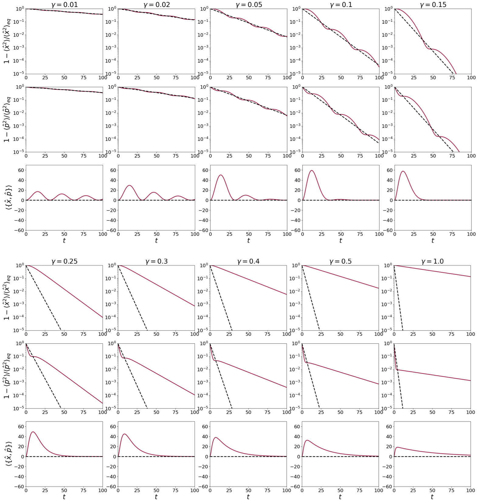
Figure 1: Time-dependence of the equal-time correlators $\langle\hat{x}^{2}(t)\rangle=C_{+}^{(x,x)}(t,t)$, $\langle\hat{p}^{2}(t)\rangle=C_{+}^{(p,p)}(t,t)$ and $2C_{+}^{(x,p)}(t,t)=\langle\bigl{\{}\hat{x}(t),\hat{p}(t)\bigr{\}}\rangle$. The system is initially prepared in the ground state $\hat{a}\left|0\right\rangle=0$ of the quantum harmonic oscillator. The full red lines refer to the friction model and the dashed black lines to the cavity model. The columns refer to different values of the damping constant $\gamma=[0.01,0.02,0.05,0.10,0.15,0.25,0.3,0.4,0.5,1.0]$, with the expected transition at $\gamma=2\omega$. The parameters $B=0$, $g=1$, $\hbar=1$, $\omega=0.1$ and $T=10$ are used.

As an example, we consider the system to be prepared in a Gaussian state, e.g. any Gibbs thermal state for $\hat{H}$, where

$$\mathcal{W}(0,\bm{r})=\frac{1}{2\pi\sqrt{\det\bm{\Gamma}\,}\,}\exp{-\frac{1}{2}(\bm{r}-\bm{\nu})^{T}\bm{\Gamma}^{-1}(\bm{r}-\bm{\nu})}$$ (IV.19)

This choice is less restrictive as it might appear at first sight, since states represented as an infinite sum of shifted gaussians are dense in the space of (square-)integrable functions (Meyer, 1992, sect. 6.6),Mazya and Schmidt (2007),Calcaterra and Boldt (2008). According to eq. (IV.10), the full solution is

$$\mathcal{W}_{\alpha}(t,\bm{r})=\frac{1}{2\pi\sqrt{\det\bm{\Omega}_{\alpha}(t)\,}\,}\exp{-\frac{1}{2}\Big{(}\bm{r}-\bm{M}_{\alpha}(t)\Big{)}^{T}\bm{\Omega}_{\alpha}^{-1}(t)\Big{(}\bm{r}-\bm{M}_{\alpha}(t)\Big{)}}$$ (IV.20)

where

$$\bm{M}_{\alpha}(t)={\rm e}^{-\bm{\Theta}_{\alpha}t}\bm{\nu}+\bm{m}_{\alpha}(t)\;\;,\;\;\bm{\Omega}_{\alpha}(t)={\rm e}^{-\bm{\Theta}_{\alpha}t}\bm{\Gamma}{\rm e}^{-\bm{\Theta}_{\alpha}^{T}t}+\bm{\Sigma}_{\alpha}(t)$$ (IV.21)

In order to compute averages, we need to evaluate

$$\int_{\mathbb{R}^{2}}\!{\rm d}\bm{r}\>g(\bm{r})\mathcal{W}_{\alpha}(t,\bm{r}) = \frac{1}{2\pi\sqrt{\det\bm{\Omega}_{\alpha}(t)\,}\,}\int_{\mathbb{R}^{2}}\!{\rm d}\bm{r}\>g\Big{(}\bm{r}+\bm{M}_{\alpha}(t)\Big{)}\exp{-\frac{1}{2}\bm{r}^{T}\bm{\Omega}_{\alpha}^{-1}(t)\bm{r}}$$ (IV.22)

$$= \exp{\frac{1}{2}\sum_{i,j=1}^{2}(\bm{\Omega}_{\alpha})_{ij}\partial_{r_{i}}\partial_{r_{j}}}g\Big{(}\bm{r}+\bm{M}_{\alpha}(t)\Big{)}\Bigg{|}_{\bm{r}=0}$$

where $g(\bm{r})$ is an arbitrary analytic function defined in phase-space. For instance, we find

$$\langle\hat{\bm{r}}\rangle_{\alpha}(t)=\bm{M}_{\alpha}(t)=\begin{pmatrix}M^{x}_{\alpha}(t)\\ M^{p}_{\alpha}(t)\end{pmatrix},\qquad\langle\hat{x}^{2}\rangle_{\alpha}(t)=\Big{(}M^{x}_{\alpha}(t)\Big{)}^{2}+\Big{(}\bm{\Omega}_{\alpha}(t)\Big{)}_{11},\qquad\langle\hat{p}^{2}\rangle_{\alpha}(t)=\Big{(}M^{p}_{\alpha}(t)\Big{)}^{2}+\Big{(}\bm{\Omega}_{\alpha}(t)\Big{)}_{22}$$ (IV.23)

From Eqs. (IV.13,IV.21), the relaxation time is expressed through the eigenvalues $\Lambda_{\pm}^{(\alpha)}$ of $\Theta_{\alpha}$. For the cavity model, $\Lambda_{\pm}^{(c)}=\gamma/2\pm{\rm i}\omega$ is always complex. Therefore the characteristic relaxation time is $2/\gamma$, since the imaginary part of $\Lambda_{\pm}^{(c)}$ merely generates an oscillatory behaviour. On the other hand, in the friction model two regimes arise: if $\gamma<2\omega$, the eigenvalues $\Lambda_{\pm}^{(f)}=(\gamma\pm{\rm i}\sqrt{4\omega^{2}-\gamma^{2}})/2$ are complex, and the relaxation time is still $2/\gamma$; but if $\gamma>2\omega$, the eigenvalues $\Lambda_{\pm}^{(f)}=(\gamma\pm\sqrt{\gamma^{2}-4\omega^{2}})/2$ are real, with the dominant relaxation time $2/(\gamma-\sqrt{\gamma^{2}-4\omega^{2}})$. The relaxation rates apply to single-point functions such as $\langle\hat{x}(t)\rangle$; for two-point functions such as $\langle\hat{x}^{2}(t)\rangle$, they are doubled.

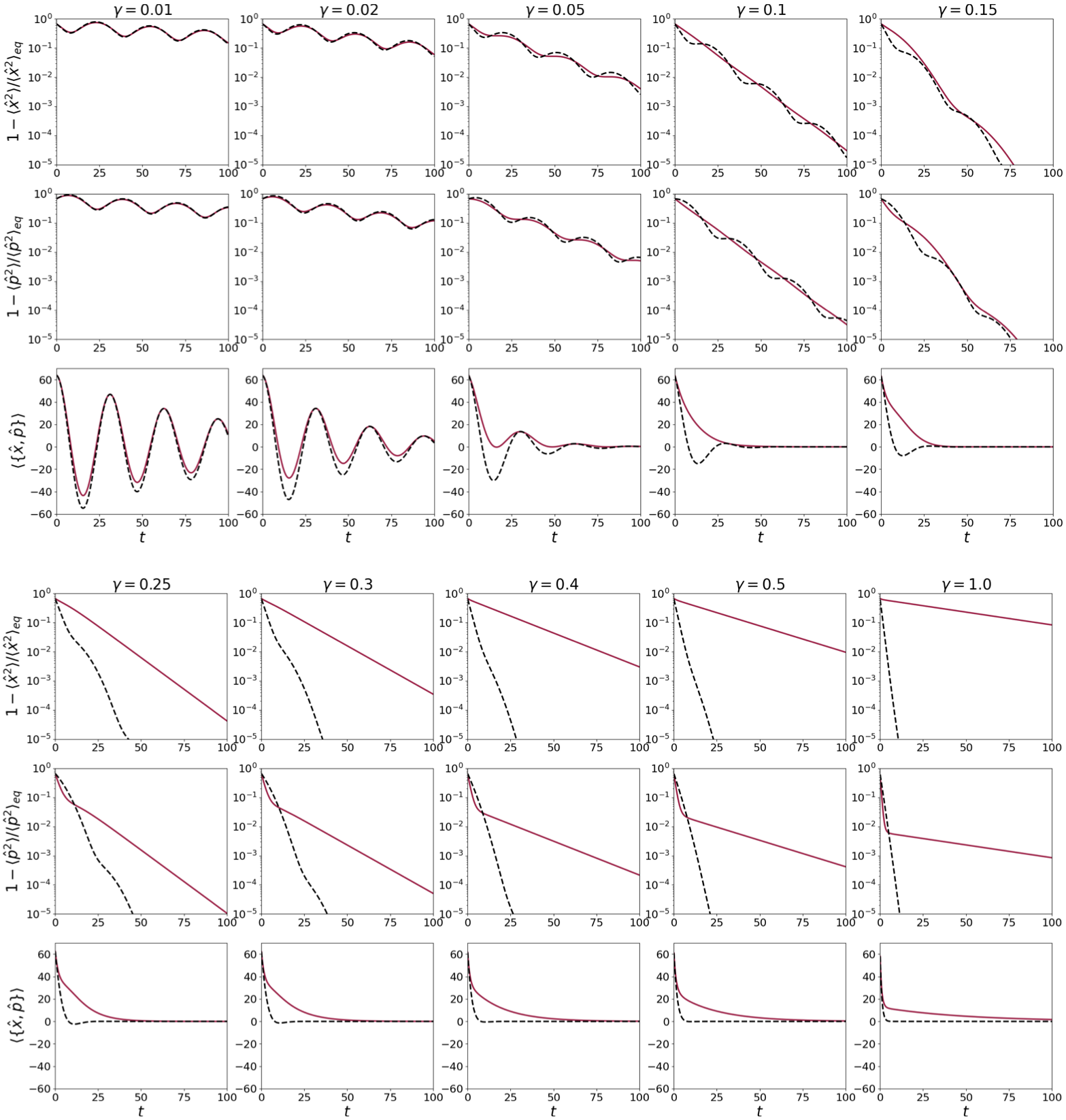
Figure 2: Time-dependence of the equal-time correlators $\langle\hat{x}^{2}(t)\rangle=C_{+}^{(x,x)}(t,t)$, $\langle\hat{p}^{2}(t)\rangle=C_{+}^{(p,p)}(t,t)$ and $2C_{+}^{(x,p)}(t,t)=\langle\bigl{\{}\hat{x}(t),\hat{p}(t)\bigr{\}}\rangle$. The system is initially prepared in the coherent state $\left|4+4{\rm i}\right\rangle$: $\hat{a}\left|4+4{\rm i}\right\rangle=(4+4{\rm i})\left|4+4{\rm i}\right\rangle$. The full red lines refer to the friction model and the dashed black lines to the cavity model. The column refer to different values of the damping constant $\gamma=[0.01,0.02,0.05,0.10,0.15,0.25,0.3,0.4,0.5,1.0]$, with the expected transition at $\gamma=2\omega$. The parameters $B=0$, $g=1$, $\hbar=1$, $\omega=0.1$ and $T=10$ are used.

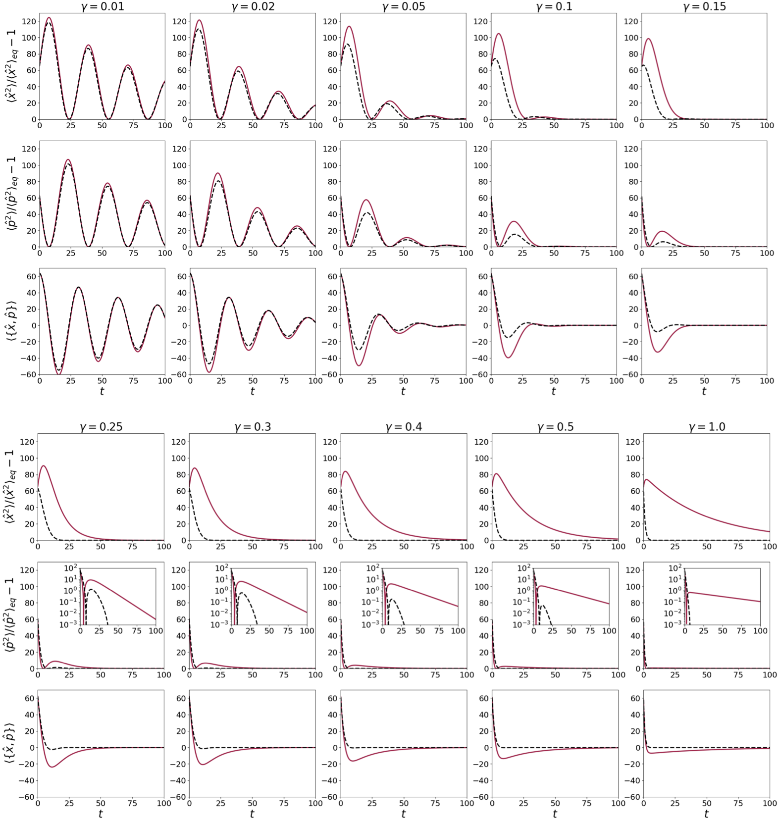
Figure 3: Time-dependence of the equal-time correlators $\langle\hat{x}^{2}(t)\rangle=C_{+}^{(x,x)}(t,t)$, $\langle\hat{p}^{2}(t)\rangle=C_{+}^{(p,p)}(t,t)$ and $2C_{+}^{(x,p)}(t,t)=\langle\bigl{\{}\hat{x}(t),\hat{p}(t)\bigr{\}}\rangle$. The system is initially prepared in the coherent state $\left|4+4{\rm i}\right\rangle$: $\hat{a}\left|4+4{\rm i}\right\rangle=(4+4{\rm i})\left|4+4{\rm i}\right\rangle$. The full red lines refer to the friction model and the dashed black lines to the cavity model. The column refer to different values of the damping constant $\gamma=[0.01,0.02,0.05,0.10,0.15,0.25,0.3,0.4,0.5,1.0]$, with the expected transition at $\gamma=2\omega$. The parameters $B=0$, $g=1$, $\hbar=1$, $\omega=0.1$ and $T=0$ are used.

The resulting relaxational behaviour of the averages $\bigl{\langle}\hat{x}^{2}\bigr{\rangle}(t)=C_{+}^{(x,x)}(t,t)$, $\bigl{\langle}\hat{x}^{2}\bigr{\rangle}(t)=C_{+}^{(x,x)}(t,t)$ and $\bigl{\langle}\bigl{\{}\hat{x}(t),\hat{p}(t)\bigr{\}}\bigr{\rangle}$ is illustrated in figures 1, 2 and 3. The upper half of each figure refers to the ‘under-damped’ regime $\gamma<2\omega$ and the lower half of each figure refers to the ‘over-damped’ regime $\gamma>2\omega$. In each half-figure there are three lines each of which displays the evolution of $\bigl{\langle}\hat{x}^{2}\bigr{\rangle}(t)$, $\bigl{\langle}\hat{p}^{2}\bigr{\rangle}(t)$ and $\bigl{\langle}\bigl{\{}\hat{x}(t),\hat{p}(t)\bigr{\}}\bigr{\rangle}$, respectively, for several values of $\gamma$. Since $B=0$, both models evolve towards the same equilibrium Gibbs state (IV.16). In figure 1, the initial state is the harmonic oscillator ground state $\hat{a}\left|0\right\rangle=0$. In figures 2 and 3, the initial state is the coherent state $\hat{a}\left|4+4{\rm i}\right\rangle=\bigl{(}4+4{\rm i}\bigr{)}\left|4+4{\rm i}\right\rangle$. The evolutions at temperature $T=10$ shown in figures 1 and 2 look globally similar, while the pure quantum evolution at $T=0$ shown in figure 3 looks different. In the cavity model, the leading relaxation time is $\tau=1/\gamma$ for all values of $\gamma$, in the friction model one has $\tau=1/\gamma$ in the ‘under-damped’ regime $\gamma<2\omega$ and in the ‘over-damped’ regime $\gamma>2\omega$, $\tau=1/\bigl{(}\gamma-\sqrt{\gamma^{2}-4\omega^{2}\,}\,\bigr{)}\simeq\omega^{2}/\gamma$ for $\gamma\gg 1$. For $\langle\hat{x}^{2}(t)\rangle$ and $\langle\hat{p}^{2}(t)\rangle$ the plots are arranged such that through the comparison with the equilibrium values the deviation with respect to equilibrium is traced. We see in figures 1 and 2 that for a large temperature $T=10$, both $\bigl{\langle}\hat{x}^{2}\bigr{\rangle}(t)\leq\bigl{\langle}\hat{x}^{2}\bigr{\rangle}_{\rm eq}$ and $\bigl{\langle}\hat{p}^{2}\bigr{\rangle}(t)\leq\bigl{\langle}\hat{p}^{2}\bigr{\rangle}_{\rm eq}$ approach their equilibrium values from below, while for $T=0$, the opposite holds true, viz. $\bigl{\langle}\hat{x}^{2}\bigr{\rangle}(t)\geq\bigl{\langle}\hat{x}^{2}\bigr{\rangle}_{\rm eq}$ and $\bigl{\langle}\hat{p}^{2}\bigr{\rangle}(t)\geq\bigl{\langle}\hat{p}^{2}\bigr{\rangle}_{\rm eq}$, hence equilibrium is approached from above, see figure 3. These observations agree with the condition (D) which stipulates that for both models the stationary states of these two observables should relax towards their equilibrium value. However, there are also important differences between the two models.

Since the lindbladian (III.1) is derived from a second-order Born approximation in $\gamma$, the presence of merely the ‘under-damped’ regime is expected in the cavity model whereas the existence of the ‘over-damped’ regime in the friction model suggests that there such an assumption should not be necessary. We also see that for $\gamma\ll 1$, the relaxation in both models is almost identical. On the other hand, qualitative differences appear with increasing values of $\gamma$ and generically, the cavity model reaches equilibrium more rapidly than the friction model. If the initial state is the ground state $\left|0\right\rangle$, the anti-commutator of the friction model is always positive and vanishes at certain specific times (it vanishes identically in the cavity model), whereas for the coherent initial state $\left|4+4{\rm i}\right\rangle$, for both models it oscillates around its equilibrium value, as predicted in the appendices A and B. For pure quantum dynamics at $T=0$, see figure 3, both $\bigl{\langle}\hat{x}^{2}\bigr{\rangle}(t)$ and $\bigl{\langle}\hat{p}^{2}\bigr{\rangle}(t)$ vanish in the ‘under-damped’ regime at certain times, which does not occur for $T=10$. The decaying oscillations in $\langle\hat{x}^{2}(t)\rangle$ and $\langle\hat{p}^{2}(t)\rangle$ are phase-shifted in such a way that a plateau in one corresponds to a maximal decay rate in the other. Forth, the anti-commutator of the friction model displays a sequence of damped oscillations such that the maxima appear to coïncide with the plateaux in the decay of $\langle\hat{p}^{2}(t)\rangle$ and the zeros with the plateaux in $\langle\hat{x}^{2}(t)\rangle$. In the ‘over-damped’ regime, there is a clear cross-over between a rapid short-time dynamics towards a more slow long-time decay, notably visible for $\bigl{\langle}\hat{p}^{2}\bigr{\rangle}(t)$ and especially in the friction model.

This clearly illustrates the notable differences in the physical behaviour of the cavity model with a completely positive Liouvillian and the friction model which is manifestly not completely positive.

V Effective mean-field theories

Mean-field descriptions Nishimori and Ortiz (2010) of phase transitions often provide a first qualitative appreciation of cooperative effects in many-body systems. In their most simple form, they arise from a replacement of interaction terms by a self-consistently determined external field. In order to further illustrate the differences between the cavity model and the friction model, we shall interpret their long-time behaviour as mean-field approximations of a many-body magnet, where the averaged position $m=\bigl{\langle}\hat{x}\bigr{\rangle}$ becomes the model’s magnetisation. As a model of reference, we shall use the the quantum spherical model, whose equilibrium and non-equilibrium critical behaviour is well-understood and shares many qualitative features with more ‘realistic’ models Berlin and Kac (1952); Lewis and Wannier (1952); Henkel and Hoeger (1984); Nieuwenhuizen (1995); Vojta (1996); Godrèche and Luck (2000); Rokni and Chandra (2004); Oliveira et al. (2006); Sachdev (2011); Chandran et al. (2013); Bienzobaz and Salinas (2013); Maraga et al. (2015); Gagel et al. (2015); Pérez-Maldonado et al. (2017); Barbier et al. (2019); Wald and Henkel (2015); Wald et al. (2018, 2021). For a recent review and tutorial, see Henkel (2023). In order to emphasise quantum effects, we set the bath temperature $T=0$. The corresponding single-particle hamiltonian is Wald and Henkel (2016)

$$\hat{H}=\hbar\omega\left(\hat{a}^{{\dagger}}\hat{a}+\frac{1}{2}\right)-B\sqrt{\frac{\hbar g}{2\omega}\,}\,\left(\hat{a}^{{\dagger}}+\hat{a}\right)$$ (V.1)

where $B$ is the external magnetic field. The angular frequency $\omega=\omega(t)$ is fixed through the spherical constraint $\bigl{\langle}\hat{x}^{2}\bigr{\rangle}=1$, which leads to

$$\omega(t)=\frac{\hbar g}{2}\left(\bigl{\langle}\hat{a}^{{\dagger}}\hat{a}^{{\dagger}}\bigr{\rangle}+\bigl{\langle}\hat{a}\hat{a}\bigr{\rangle}+\bigl{\langle}\hat{a}^{{\dagger}}\hat{a}\bigr{\rangle}+1\right)$$ (V.2)

The interpretation of this single-body problem as an effective mean-field approximation is completed through a self-consistent form of the magnetic field

$$B=\kappa\bigl{\langle}x\bigr{\rangle}=\kappa\sqrt{\frac{\hbar g}{2\omega}\,}\,\bigl{\langle}\hat{a}^{{\dagger}}+\hat{a}\bigr{\rangle}=\kappa\sqrt{\frac{2\hbar g}{\omega}\,}\,x_{1}$$ (V.3)

where $\kappa>0$ is the molecular field constant.

The equations of motion of both the friction and the cavity model can be taken from appendix C, using also (V.3), where for simplicity we use the notations

$$\bigl{\langle}\hat{a}\bigr{\rangle}=x_{1}+{\rm i}x_{2}\;\;,\;\;\bigl{\langle}\hat{a}\hat{a}\bigr{\rangle}=x_{3}+{\rm i}x_{4}\;\;,\;\;\bigl{\langle}\hat{a}^{{\dagger}}\hat{a}\bigr{\rangle}=x_{5}$$ (V.4)

and the spherical constraint (V.2) is used to eliminate $x_{5}$. We are interested in the phase diagramme of the stationary state and shall use from now on $\omega:=\lim_{t\to\infty}\omega(t)$. Since solving the stationary equations of motion is straightforward, we now briefly state the results.

V.1 Friction model

Two distinct stationary solutions are found. They are independent of $\gamma$, as it should be for a stationary state at equilibrium. The first one corresponds to a disordered, paramagnetic state with $x_{1}=x_{2}=x_{3}=x_{4}=x_{5}=0$ and $\omega=\omega_{d}={\hbar g}/{2}$. The magnetisation $m=0$ vanishes. The second one corresponds to an ordered, magnetic state with $x_{1}\neq 0$ and $\omega=\omega_{o}=\sqrt{\kappa g\,}$. It reads $x_{2}=x_{4}=0$ and

$$m^{2}=x_{1}^{2}=\frac{1}{4\sqrt{g\,}}\left(\frac{2\sqrt{\kappa\,}}{\hbar}-\sqrt{g\,}\right)=x_{3}$$ (V.5)

At the critical point, $\omega_{d}=\omega_{o}$ which gives the critical value $g_{c}={4\kappa}/{\hbar}^{2}$. Then the magnetisation become $m^{2}=\bigl{(}g_{c}^{1/2}-g^{1/2}\bigr{)}/4g^{1/2}$ such that the system is magnetically ordered for all $g<g_{c}$, as expected for an ordered magnetic state at equilibrium, see figure 4. Since close to criticality, one expects $m^{2}\sim\bigl{(}g_{c}-g\bigr{)}^{2\beta}$, one recovers the standard mean-field exponent $\beta=\frac{1}{2}$.

Figure 4: Mean-field phase diagrammes of a single quantum spherical spin at $T=0$, for the cavity model (left) and the friction model (right).

V.2 Cavity model

Again, two distinct stationary solutions are found Wald and Henkel (2016). The first one is identical to the disordered solution $x_{1}=x_{2}=x_{3}=x_{4}=x_{5}=0$ and $\omega=\omega_{d}={\hbar g}/{2}$ of the friction model. The second solution, however, is now $\gamma$-dependent and $\omega_{o}^{\prime}=\sqrt{g\kappa-\gamma^{2}/4\,}$. Then all $x_{1},\ldots,x_{4}$ are non-vanishing. The condition of criticality $\omega_{d}=\omega_{o}^{\prime}$ now has two solutions for $\gamma<2\kappa/\hbar$, which leads to two separate critical points Wald and Henkel (2016)

$$g_{c,\pm}(\gamma)=\frac{2\kappa}{\hbar^{2}}\pm\sqrt{\frac{4\kappa^{2}}{\hbar^{4}}-\frac{\gamma^{2}}{\hbar^{2}}\,}\simeq\left\{\begin{array}[]{l}4\kappa/\hbar^{2}\\[1.42271pt] \gamma^{2}/4\kappa\end{array}\right.$$ (V.6)

along with their leading behaviour for $\gamma\to 0$. While in the limit $\gamma\to 0$, the upper critical point $\lim_{\gamma\to 0}g_{c,+}(\gamma)=g_{c}$ goes over into the one of the friction model, for a finite $\gamma<2\kappa/\hbar$, there is also a lower critical point $g_{c,-}(\gamma)$. This is shown in figure 4. The magnetisation reads Wald and Henkel (2016)

$$m^{2}=x_{1}^{2}=\frac{\gamma^{2}}{4\kappa g}\left(1+\frac{4\omega^{2}}{\gamma}\right)\left(1-\frac{\hbar g}{2\omega}\right)$$ (V.7)

and is non-vanishing only between $g_{c,-}(\gamma)<g<g_{c,+}(\gamma)$. These re-entrant transitions are a purely kinetic effect and cannot be properties of an equilibrium state. Through the value of damping constant, the cavity strongly influences the behaviour even of the stationary state.

Hence this simple example shows that the cavity model dynamics does not describe relaxations to an equilibrium state, in contrast to the friction model. This is a consequence of the distinct effective hamiltonians when $B\neq 0$, as seen in eq. (IV.17).

VI Discussion and conclusion

In this work, we explored characteristics of the dynamics of open quantum systems where the relaxation times of the bath(s) are short enough such that an effective markovian description becomes sensible. Rather than modelling both the system and the bath(s), and also their interactions, one rather seeks a reduced formulation which contains explicitly only the degrees of freedom of the system, along with a few parameters to describe the bath(s) interacting with the system. A commonly used formulation uses a master equation for the density matrix. If written in a Lindblad form, such a master equation guarantees the dynamical semi-group property. However, a Lindblad master equation does contain hidden assumptions, notably on the initial correlations between the physical system and the bath. If satisfied, these directly lead to a completely positive form of the Liouvillian. On a more phenomenological level, an alternative description in terms of stochastic Langevin equation does involve an explicit assumption on admissible dissipative terms in the equations of motion and then uses physical criteria to fix the correlations of the noise operators. This kind of approach concentrates on the system and questions concerning complete positivity are not raised.

A a case study based on a single harmonic oscillator, we defined two models, the friction model and the cavity model, specified in eqs. (II.3) and (II.4), respectively. They differ in the explicit form on the non-stochastic dissipative terms but do use the same physical criteria (A-D) to fix the noise correlators. While the classical $\hbar\to 0$ limit of the friction model reduces to an ohmically damped particle in a harmonic potential subject to white noise, no known classical system emerges for the cavity model. From these Langevin equations, the equivalent Lindblad-type master equations are derived, by requiring identical equations of motion for one-point and two-point functions. The lindbladian is completely positive for the cavity model but only positive in the friction model. Reformulating the master equation as a Fokker-Planck equation, using the Wigner function formalism, shows that without an external field $B$, both models evolve towards the same Gibbs state. Explicit solutions of the equations of motion clearly illustrate the differences in the dynamics, notably through a direct study of the relaxation behaviour summarised in figures 1, 2 and 3 with distinct ‘under-damped’ and ‘over-damped’ regimes in the friction model but only an ‘under-damped’ regime in the cavity model. Alternatively, when recast as mean-field approximation of a magnetic system, the models are distinguished through a determination of the stationary state in an external field and the ensuing phase transition, see figure 4. In the limit of weak damping $\gamma\ll 1$, both models lead to the same phenomenology of time-dependent averages.

From a formal point of view, there is no obvious criterion which would permit to choose between these models (or any other one with yet different dissipative terms). The naturally-looking requirement of complete positivity is not always convincing, and has the disadvantage that the cavity model in the classical limit $\hbar\to 0$ does not lead back to a classical brownian particle in a harmonic potential. Beyond our purely phenomenological discussion, it would be satisfying to derive microscopically the contribution $\hat{H}_{\gamma}$ to the effective hamiltonian and/or the explicit form of the Lindblad dissipator $\mathcal{D}(\hat{\rho}(t))$. This study is also meant as a preparation to study to many-body dynamics, notably the quantum spherical model, since its hamiltonian can be reduced to a sum of bosonic harmonic oscillators, see Henkel (2023) and refs. therein. Still, in that model the spherical constraint renders the dynamics non-trivial, e.g. Wald and Henkel (2016). The study of relaxational dynamics in the markovian approximation of many-body systems and the comparison with the results of full quantum dynamics (respecting the qfdt), e.g. Chandran et al. (2013); Sieberer et al. (2015); Barbier et al. (2019); Wald et al. (2021), will be taken up elsewhere.

Acknowledgements: It is a pleasure to thank D. Karevski and G.T. Landi for useful discussions. This work was supported by ANR-PRME UNIOPEN (ANR-22-CE30-0004-01). One of us (M.C.) thanks the LUE for funding a travel grant (Aide à la mobilité internationale DrEAM).

Appendix A. Noise correlators for the cavity model

We outline the solution of (II.9) and subsequently, the derivation of the second moments (II.4) from the conditions (A-D).

The lines of calculation follow closely Araújo et al. (2019). Considering first the homogeneous part of (II.9), we have the relaxation rates $\Lambda_{\pm}=\frac{\gamma}{2}\pm{\rm i}\omega$ such that we can make the ansatz

$$\hat{x}(t)=\hat{x}_{+}(t)\,{\rm e}^{-\Lambda_{+}t}+\hat{x}_{-}(t)\,{\rm e}^{-\Lambda_{-}t}\;\;,\;\;\hat{p}(t)=\hat{p}_{+}(t)\,{\rm e}^{-\Lambda_{+}t}+\hat{p}_{-}(t)\,{\rm e}^{-\Lambda_{-}t}$$ (A.1)

Two of the four amplitudes in the above ansatz may still be chosen freely. Our choice is $\hat{p}_{\pm}(t)=-\frac{1}{g}\bigl{(}\Lambda_{\pm}-\frac{\gamma}{2}\bigr{)}\hat{x}_{\pm}(t)=\mp\frac{{\rm i}\omega}{g}\hat{x}_{\pm}(t)$. Insertion of the ansatz into (II.4a) leads to

$$\partial_{t}\hat{x}_{+}(t)\,{\rm e}^{-\Lambda_{+}t}+\partial_{t}\hat{x}_{+}(t)\,{\rm e}^{-\Lambda_{+}t}=\hat{\eta}^{(x)}(t)\;\;,\;\;-\frac{{\rm i}\omega}{g}\partial_{t}\hat{x}_{+}(t)\,{\rm e}^{-\Lambda_{+}t}+\frac{{\rm i}\omega}{g}\partial_{t}\hat{x}_{+}(t)\,{\rm e}^{-\Lambda_{+}t}=B+\hat{\eta}^{(p)}(t)$$ (A.2)

From these, we directly have

$$\partial_{t}\hat{x}_{\pm}(t)=\frac{1}{2}\left(\hat{\eta}^{(x)}(t)\pm\frac{{\rm i}g}{\omega}\left(\hat{\eta}^{(p)}+B\right)\right)\,e^{\Lambda_{\pm}t}$$ (A.3)

which upon integration produces

$$\hat{x}(t) =\hat{x}_{+}(0){\rm e}^{-\Lambda_{+}t}+\hat{x}_{-}(0){\rm e}^{-\Lambda_{-}t}+\frac{1}{2}\int_{0}^{t}\!{\rm d}\tau\>{\rm e}^{-\Lambda_{+}(t-\tau)}\left(\hat{\eta}^{(x)}(\tau)+\frac{{\rm i}g}{\omega}\left(\hat{\eta}^{(p)}(\tau)+B\right)\right)+\frac{1}{2}\int_{0}^{t}\!{\rm d}\tau\>{\rm e}^{-\Lambda_{-}(t-\tau)}\left(\hat{\eta}^{(x)}(\tau)-\frac{{\rm i}g}{\omega}\left(\hat{\eta}^{(p)}(\tau)+B\right)\right)$$ (A.4a)

$$\hat{p}(t) =-{\rm i}\frac{\omega}{g}\hat{x}_{+}(0){\rm e}^{-\Lambda_{+}t}+{\rm i}\frac{\omega}{g}\hat{x}_{-}(0){\rm e}^{-\Lambda_{-}t}$$

$$\leavevmode\nobreak\ \leavevmode\nobreak\ \leavevmode\nobreak\ \leavevmode\nobreak\ -{\rm i}\frac{\omega}{2g}\int_{0}^{t}\!{\rm d}\tau\>{\rm e}^{-\Lambda_{+}(t-\tau)}\left(\hat{\eta}^{(x)}(\tau)+\frac{{\rm i}g}{\omega}\left(\hat{\eta}^{(p)}(\tau)+B\right)\right)+{\rm i}\frac{\omega}{2g}\int_{0}^{t}\!{\rm d}\tau\>{\rm e}^{-\Lambda_{-}(t-\tau)}\left(\hat{\eta}^{(x)}(\tau)-\frac{{\rm i}g}{\omega}\left(\hat{\eta}^{(p)}(\tau)+B\right)\right)$$ (A.4b)

as quoted in (II.10) in the main text for the special case $B=0$.

The second moments (II.4) of the noises are found as follows. For the averaged noise commutator, we make the ansatz $\bigl{\langle}\left[\hat{\eta}(^{(x)}t),\hat{\eta}^{(p)}(t^{\prime})\right]\bigr{\rangle}=\kappa\delta(t-t^{\prime})$. Then, consider the commutator, computed using (A.4)

$$2C_{-}^{(x,p)}(t,t^{\prime})=\bigl{\langle}\left[\hat{x}(t),\hat{p}(t^{\prime})\right]\bigr{\rangle}=\left(\frac{{\rm i}\omega}{g}\bigl{\langle}\left[\hat{x}_{+}(0),\hat{x}_{-}(0)\right]\bigr{\rangle}-\frac{\kappa}{2\gamma}\right)\left({\rm e}^{-\Lambda_{+}t-\Lambda_{-}t^{\prime}}+{\rm e}^{-\Lambda_{-}t-\Lambda_{+}t^{\prime}}\right)+\frac{\kappa}{2\gamma}\left({\rm e}^{-\Lambda_{+}|t-t^{\prime}|}+{\rm e}^{-\Lambda_{-}|t-t^{\prime}|}\right)$$ (A.5)

which contains a stationary part depending only on $|t-t^{\prime}|$ and a rapidly decaying transient part. In order to achieve the equal-time canonical position-momentum commutator, the transient term must vanish which is achieved through the choice

$$\bigl{\langle}\left[\hat{x}_{+}(0),\hat{x}_{-}(0)\right]\bigr{\rangle}=\frac{1}{{\rm i}}\frac{\kappa g}{2\gamma\omega}$$ (A.6)

Then the averaged equal-time commutator $\bigl{\langle}\left[\hat{x}(t),\hat{p}(t)\right]\bigr{\rangle}=\frac{\kappa}{\gamma}$ is indeed a time-independent constant which is fixed to its canonical value by choosing $\kappa={\rm i}\hbar\gamma$, which is (II.4b) in the main text.

Next, we check the Kubo formula. On one side, with the definitions (II.5), we obtain

$$\partial_{t}R^{(x)}(t,s)=gQ^{(p)}(t,s)-\frac{\gamma}{2}R^{(x)}(t,s)\;\;,\;\;\partial_{t}Q^{(p)}(t,s)=-\frac{\omega^{2}}{g}R^{(x)}(t,s)-\frac{\gamma}{2}Q^{(p)}(t,s)+\delta(t-s)$$ (A.7)

Since these will only depend on the time difference $\tau=t-s$, we define $\mathscr{R}(\tau):=R^{(x)}(t,s)$ which obeys the second-order equation

$$\partial_{\tau}^{2}\mathscr{R}(\tau)+\gamma\partial_{\tau}\mathscr{R}(\tau)+\left(\omega^{2}+\frac{\gamma^{2}}{4}\right)\mathscr{R}(\tau)=g\delta(\tau)$$ (A.8)

Using the Fourier transform $\widehat{\mathscr{R}}(\nu)=\frac{1}{\sqrt{2\pi\,}}\int_{\mathbb{R}}\!{\rm d}\tau\>{\rm e}^{-{\rm i}\nu\tau}\mathscr{R}(\tau)$, we find

$$\widehat{\mathscr{R}}(\nu)=-\frac{g}{\sqrt{2\pi\,}}\frac{1}{\nu^{2}-{\rm i}\gamma\nu-\omega^{2}-\gamma^{2}/4}$$ (A.9)

whose pôles $\nu_{\pm}={\rm i}\frac{\gamma}{2}\pm\omega$ are in the upper complex $\nu$-half-plane. Consequently, inverting (A.9) via the residue theorem, the response of the position $x$ is

$$\mathscr{R}(\tau)=R^{(x)}(\tau+s,s)=\frac{g}{\omega}\,{\rm e}^{-\gamma\tau/2}\sin\bigl(\omega\tau\bigr{missing})\>\Theta\bigl{(}\tau\bigr{)}$$ (A.10)

where the Heaviside function $\Theta(\tau)$ expresses the expected causality. On the other had, we need the commutator (II.6)

$$C_{-}^{(x,x)}(t,t^{\prime})=\frac{1}{2}\underbrace{\left(\bigl{\langle}\bigl{[}\hat{x}_{+}(0),\hat{x}_{-}(0)\bigr{]}\bigr{\rangle}-\frac{\hbar g}{2\omega}\right)}_{=0}\left({\rm e}^{-\Lambda_{+}t-\Lambda_{-}t^{\prime}}-{\rm e}^{-\Lambda_{+}t^{\prime}-\Lambda_{-}t}\right)+\frac{\hbar}{2{\rm i}}\frac{g}{\omega}{\rm e}^{-\gamma|t-t^{\prime}|/2}\sin\bigl(\omega|t-t^{\prime}|\bigr{missing})$$ (A.11)

This is stationary because of (A.6) with $\kappa={\rm i}\hbar\gamma$. Hence the Kubo formula $R^{(x)}(\tau+s,s)=\frac{2{\rm i}}{\hbar}C_{-}^{(x,x)}(\tau+s,s)\Theta(\tau)$ is automatically satisfied.

Finally, we analyse the virial theorem. If $B\neq 0$, we must analyse the connected correlators $C_{+,{\rm c}}^{(x,x)}(t,t^{\prime}):=\frac{1}{2}\left\langle\left\{\hat{x}(t),\hat{x}(t^{\prime})\right\}\right\rangle-\left\langle\hat{x}(t)\right\rangle\left\langle\hat{x}(t^{\prime})\right\rangle$ and analogously for $C_{+,{\rm c}}^{(p,p)}(t,t^{\prime}):=\frac{1}{2}\left\langle\left\{\hat{p}(t),\hat{p}(t^{\prime})\right\}\right\rangle-\left\langle\hat{p}(t)\right\rangle\left\langle\hat{p}(t^{\prime})\right\rangle$. In the case at hand, the virial theorem requires that for the stationary contributions $C_{+,{\rm c,stat}}^{(p,p)}(t,t^{\prime})=\frac{\omega^{2}}{g^{2}}C_{+,{\rm c,stat}}^{(x,x)}(t,t^{\prime})$. Following Araújo et al. (2019), in order to work out the correlators, we assume that the second moments read

$$\frac{1}{2}\bigl{\langle}\left\{\hat{\eta}^{(p)}(t),\hat{\eta}^{(p)}(t^{\prime})\right\}\bigr{\rangle}=\alpha\,\delta(t-t^{\prime})\;\;,\;\;\frac{1}{2}\bigl{\langle}\left\{\hat{\eta}^{(x)}(t),\hat{\eta}^{(x)}(t^{\prime})\right\}\bigr{\rangle}=\beta\,\delta(t-t^{\prime})\;\;,\;\;\bigl{\langle}\left\{\hat{\eta}^{(x)}(t),\hat{\eta}^{(p)}(t^{\prime})\right\}\bigr{\rangle}=0$$ (A.12)

In order to find the constants $\alpha,\beta$, using the above definition, we must calculate first

$$C_{+,{\rm c}}^{(x,x)}(t,t^{\prime}) = \left(\bigl{\langle}\hat{x}_{+}(0)^{2}\bigr{\rangle}-\frac{\beta-\alpha g^{2}/\omega^{2}}{8\Lambda_{+}}\right){\rm e}^{-\Lambda_{+}(t+t^{\prime})}+\left(\bigl{\langle}\hat{x}_{-}(0)^{2}\bigr{\rangle}-\frac{\beta-\alpha g^{2}/\omega^{2}}{8\Lambda_{-}}\right){\rm e}^{-\Lambda_{-}(t+t^{\prime})}$$ (A.13)

$$+\left(\frac{1}{2}\bigl{\langle}\bigl{\{}\hat{x}_{+}(0),\hat{x}_{-}(0)\bigr{\}}\bigr{\rangle}-\frac{\beta+\alpha g^{2}/\omega^{2}}{4(\Lambda_{+}+\Lambda_{-})}\right)\left({\rm e}^{-\Lambda_{+}t-\Lambda_{-}t^{\prime}}+{\rm e}^{-\Lambda_{+}t^{\prime}-\Lambda_{-}t}\right)$$

$$+\frac{1}{4}\left(\frac{\beta-\alpha g^{2}/\omega^{2}}{2\Lambda_{+}}+\frac{\beta+\alpha g^{2}/\omega^{2}}{\Lambda_{+}+\Lambda_{-}}\right){\rm e}^{-\Lambda_{+}|t-t^{\prime}|}+\frac{1}{4}\left(\frac{\beta-\alpha g^{2}/\omega^{2}}{2\Lambda_{-}}+\frac{\beta+\alpha g^{2}/\omega^{2}}{\Lambda_{+}+\Lambda_{-}}\right){\rm e}^{-\Lambda_{-}|t-t^{\prime}|}$$

The terms in the first two lines are rapidly decaying transient terms whereas the stationary terms are collected in the third line and the non-connected terms $\sim B^{2}$ cancelled. Second, we similarly find

$$C_{+,{\rm c}}^{(p,p)}(t,t^{\prime}) = \frac{\omega^{2}}{g^{2}}\left(-\bigl{\langle}\hat{x}_{+}(0)^{2}\bigr{\rangle}+\frac{\beta-\alpha g^{2}/\omega^{2}}{8\Lambda_{+}}\right){\rm e}^{-\Lambda_{+}(t+t^{\prime})}+\frac{\omega^{2}}{g^{2}}\left(-\bigl{\langle}\hat{x}_{-}(0)^{2}\bigr{\rangle}+\frac{\beta-\alpha g^{2}/\omega^{2}}{8\Lambda_{-}}\right){\rm e}^{-\Lambda_{-}(t+t^{\prime})}$$ (A.14)

$$+\frac{\omega^{2}}{g^{2}}\left(\frac{1}{2}\bigl{\langle}\bigl{\{}\hat{x}_{+}(0),\hat{x}_{-}(0)\bigr{\}}\bigr{\rangle}-\frac{\beta+\alpha g^{2}/\omega^{2}}{4(\Lambda_{+}+\Lambda_{-})}\right)\left({\rm e}^{-\Lambda_{+}t-\Lambda_{-}t^{\prime}}+{\rm e}^{-\Lambda_{+}t^{\prime}-\Lambda_{-}t}\right)$$

$$+\frac{\omega^{2}}{4g^{2}}\left(-\frac{\beta-\alpha g^{2}/\omega^{2}}{2\Lambda_{+}}+\frac{\beta+\alpha g^{2}/\omega^{2}}{\Lambda_{+}+\Lambda_{-}}\right){\rm e}^{-\Lambda_{+}|t-t^{\prime}|}+\frac{\omega^{2}}{4g^{2}}\left(-\frac{\beta-\alpha g^{2}/\omega^{2}}{2\Lambda_{-}}+\frac{\beta+\alpha g^{2}/\omega^{2}}{\Lambda_{+}+\Lambda_{-}}\right){\rm e}^{-\Lambda_{-}|t-t^{\prime}|}$$

with transient terms in the first two lines and the stationary contributions in the last line. Comparing (A.13,A.14), we see that the virial theorem is satisfied if and only if

$$\frac{1}{4}\left(\frac{\beta-\alpha g^{2}/\omega^{2}}{2\Lambda_{\pm}}+\frac{\beta+\alpha g^{2}/\omega^{2}}{\Lambda_{+}+\Lambda_{-}}\right)\stackrel{{\scriptstyle!}}{{=}}\frac{1}{4}\left(-\frac{\beta-\alpha g^{2}/\omega^{2}}{2\Lambda_{\pm}}+\frac{\beta+\alpha g^{2}/\omega^{2}}{\Lambda_{+}+\Lambda_{-}}\right)$$ (A.15)

which leads to

$$\alpha=\frac{\omega^{2}}{g^{2}}\beta$$ (A.16)

At last, the condition (D) specifies that the position (connected) auto-correlator at equilibrium should be (using the stationary part of (A.13))

$$C_{+,{\rm c,eq}}^{(x,x)}(t,t)=\frac{\beta}{2\gamma}\stackrel{{\scriptstyle!}}{{=}}\frac{\hbar g}{2\omega}\coth\left(\frac{\hbar\omega}{2T}\right)$$ (A.17)

which implies $\beta=\frac{\hbar\gamma\omega}{g}\coth\left(\frac{\hbar\omega}{2T}\right)$. With (A.12) this finally reproduces eqs. (II.4c,II.4d) in the main text.

To finish, we also give the anti-commutator which once more follows from (A.4). Using (A.16), we find

$$C_{+,{\rm c}}^{(x,p)}(t,t^{\prime}) = -{\rm i}\frac{\omega}{g}\bigl{\langle}\hat{x}_{+}(0)^{2}\bigr{\rangle}{\rm e}^{-\Lambda_{+}(t+t^{\prime})}+{\rm i}\frac{\omega}{g}\bigl{\langle}\hat{x}_{-}(0)^{2}\bigr{\rangle}{\rm e}^{-\Lambda_{-}(t+t^{\prime})}$$ (A.18)

$$+{\rm i}\frac{\omega}{2g}\left(\bigl{\langle}\bigl{\{}\hat{x}_{+}(0),\hat{x}_{-}(0)\bigr{\}}\bigr{\rangle}-\frac{\beta}{\gamma}\right)\left({\rm e}^{-\Lambda_{+}t-\Lambda_{-}t^{\prime}}-{\rm e}^{-\Lambda_{-}t-\Lambda_{+}t^{\prime}}\right)+{\rm i}\frac{\omega\beta}{2\gamma g}\left({\rm e}^{-\Lambda_{+}|t-t^{\prime}|}-{\rm e}^{-\Lambda_{-}|t-t^{\prime}|}\right)$$

The stationary equal-time contribution $C_{+,{\rm c,stat}}^{(x,p)}(t,t)=0$ vanishes, in agreement with the results in figures 1,2,3.

Appendix B. Anti-commutator in the friction model

In the main text, the solutions (II.8) for position and momentum were quoted. With respect to Araújo et al. (2019), we add the explicit expression for the connected anti-commutator $C_{+,{\rm c}}^{(x,p)}(t,t^{\prime}):=C_{+}^{(x,p)}(t,t^{\prime})-\left\langle\hat{x}(t)\right\rangle\left\langle\hat{p}(t^{\prime})\right\rangle$ which reads

$$C_{+,{\rm c}}^{(x,p)}(t,t^{\prime}) = \left(-\frac{\Lambda_{+}}{g}\bigl{\langle}\hat{x}_{+}(0)^{2}\bigr{\rangle}+\frac{g\alpha}{2(\Lambda_{+}-\Lambda_{-})^{2}}\right){\rm e}^{-\Lambda_{+}(t+t^{\prime})}+\left(-\frac{\Lambda_{-}}{g}\bigl{\langle}\hat{x}_{-}(0)^{2}\bigr{\rangle}+\frac{g\alpha}{2(\Lambda_{+}-\Lambda_{-})^{2}}\right){\rm e}^{-\Lambda_{-}(t+t^{\prime})}$$ (B.1)

$$-\left(\frac{1}{2g}\bigl{\langle}\bigl{\{}\hat{x}_{+}(0),\hat{x}_{-}(0)\bigr{\}}\bigr{\rangle}+\frac{g\alpha}{\gamma(\Lambda_{+}-\Lambda_{-})^{2}}\right)\Big{(}\Lambda_{-}{\rm e}^{-\Lambda_{+}t-\Lambda_{-}t^{\prime}}+\Lambda_{+}{\rm e}^{-\Lambda_{-}t-\Lambda_{+}t^{\prime}}\Big{)}$$

$$+\frac{g\alpha}{\gamma(\Lambda_{+}-\Lambda_{-})^{2}}\left(\Lambda_{-}-\frac{\gamma}{2}\right){\rm e}^{-\Lambda_{+}|t-t^{\prime}|}+\frac{g\alpha}{\gamma(\Lambda_{+}-\Lambda_{-})^{2}}\left(\Lambda_{+}-\frac{\gamma}{2}\right){\rm e}^{-\Lambda_{-}|t-t^{\prime}|}$$

with the same generic form (A.12) for the noises, $\alpha=\frac{\gamma\hbar\omega}{g}\coth\left(\frac{\hbar\omega}{2T}\right)$, $\beta=0$ Araújo et al. (2019) and recall $\Lambda_{\pm}=\frac{\gamma}{2}\pm\sqrt{\frac{\gamma^{2}}{4}-\omega^{2}\,}$. The stationary terms in last line of eq. (B.1) vanish for equal times, viz. $C_{+,{\rm c,stat}}^{(x,p)}(t,t)=0$, in agreement with the results in figures 1,2,3.

Appendix C. Formal solution of equations of motion

The five equations of motion (II.11,II.12,II.16,II.17) can be compactly written in a matrix form

$$\partial_{t}\bm{v}=\bm{A}\bm{v}+\bm{b}\;\;,\;\;\bm{v}:=\begin{pmatrix}\langle\hat{a}\rangle\\ \langle\hat{a}^{\dagger}\rangle\\ \langle\hat{a}\hat{a}\rangle\\ \langle\hat{a}^{\dagger}\hat{a}^{\dagger}\rangle\\ \langle\hat{a}^{\dagger}\hat{a}\rangle\end{pmatrix},$$ (C.1)

such that the formal solution can be written as

$$\bm{v}(t)=e^{\bm{A}t}\,\left(\bm{v}(0)+\bm{A}^{-1}\bm{b}\right)-\bm{A}^{-1}\bm{b}$$ (C.2)

For the friction model, one has for the matrix $\bm{A}$ and the vector $\bm{b}$

$$\bm{A}=\gamma\begin{pmatrix}-\frac{1}{2}&\frac{1}{2}&0&0&0\\ \frac{1}{2}&-\frac{1}{2}&0&0&0\\ 0&0&-1&0&1\\ 0&0&0&-1&1\\ 0&0&\frac{1}{2}&\frac{1}{2}&-1\end{pmatrix}+{\rm i}\begin{pmatrix}-\omega&0&0&0&0\\ 0&\omega&0&0&0\\ \sqrt{2g/\omega\hbar\,}\,B&0&-2\omega&0&0\\ 0&-\sqrt{2g/\omega\hbar\,}\,B&0&2\omega&0\\ -\sqrt{g/2\omega\hbar\,}\,B&\sqrt{g/2\omega\hbar\,}\,B&0&0&0\end{pmatrix}\;\;,\;\;\bm{b}=\gamma n_{\omega}\begin{pmatrix}0\\ 0\\ -1\\ -1\\ 1\end{pmatrix}+{\rm i}\sqrt{\frac{g}{2\omega\hbar}\,}\,B\begin{pmatrix}1\\ -1\\ 0\\ 0\\ 0\end{pmatrix},$$ (C.3)

and $n_{\omega}=(e^{\hbar\omega/T}-1)^{-1}$ is the Bose-Einstein distribution. For the cavity model, these read

$$\bm{A}=\gamma\begin{pmatrix}-\frac{1}{2}&0&0&0&0\\ 0&-\frac{1}{2}&0&0&0\\ 0&0&-1&0&0\\ 0&0&0&-1&0\\ 0&0&0&0&-1\end{pmatrix}+{\rm i}\begin{pmatrix}-\omega&0&0&0&0\\ 0&\omega&0&0&0\\ \sqrt{2g/\omega\hbar\,}\,B&0&-2\omega&0&0\\ 0&-\sqrt{2g/\omega\hbar\,}\,B&0&2\omega&0\\ -\sqrt{g/2\omega\hbar\,}\,B&\sqrt{g/2\omega\hbar\,}\,B&0&0&0\end{pmatrix}\;\;,\;\;\bm{b}=\gamma n_{\omega}\begin{pmatrix}0\\ 0\\ 0\\ 0\\ 1\end{pmatrix}+{\rm i}\sqrt{\frac{g}{2\omega\hbar}\,}\,B\begin{pmatrix}1\\ -1\\ 0\\ 0\\ 0\end{pmatrix}.$$ (C.4)

and one notices the simplifications in the real parts of $\bm{A}$ and of $\bm{b}$ in the cavity model.

Appendix D. Impossibility of complete positivity in the friction model

We try to solve the conditions (III.10) for the $\alpha_{j}$, $\beta_{j}$, with the definitions (III.7) and the additional assumption $\varepsilon_{1}=\varepsilon_{2}=+1$.

First, the conditions (III.10b,III.10c) imply that

$$E_{3}=E_{4}^{*}=\frac{1}{2}\bigl{(}E_{1}+E_{2}\bigr{)}$$ (D.1)

From the definitions (III.7) it then follows that

$$\sum_{j=1,2}\bigl{|}\alpha_{j}-\beta_{j}^{*}\bigr{|}^{2}=0$$ (D.2)

hence $\alpha_{1}=\beta_{1}^{*}$ and $\alpha_{2}=\beta_{2}^{*}$. Again using (III.7), this would imply $E_{1}=E_{2}$ which is in contradiction with (III.10a) for $\gamma>0$. Hence there is no solution and $\varepsilon_{1}=\varepsilon_{2}=+1$ is inadmissible.

Consequently, the friction model cannot be completely positive.

Appendix E. Phase-space formulation of quantum mechanics

The phase-space formulation of quantum mechanics, introduced by Wigner Wigner (1932), is attractive because of its similarity to classical hamiltonian dynamics. It is based on mapping quantum states to quasi-probability distribution functions and the Weyl transform, which maps quantum operators into real-valued functions defined on phase-space $(x,p)$. This facilitates connections to classical mechanics and semi-classical limits Moyal (1949); Hillery et al. (1984); Lee (1995); Schleich (2001); Case (2008).

Quantum observables can be represented by hermitian operators acting on the Hilbert space of system states, such that the outcome of a measurement must be an eigenvalue of the observable. Quantisation establishes a map between classical variables and quantum operators, such that the canonical commutation relation $[\hat{x},\hat{p}]=i\hbar$ between position $\hat{x}$ and momentum $\hat{p}$ hold true. However, for observables non-linear in position and momentum the ordering is ambiguous. Hence one must define a one-to-one map $\Phi[\hat{f}]=f(x,p)$ between Hilbert space operators and analytic phase-space functions. The existence of the inverse transform $\Phi^{-1}$ is guaranteed by the one-to-one correspondence. One needs a ‘product’ $\star$ between two Hilbert space operators $\hat{f}$, $\hat{g}$ which in the phase-space formalism must satisfy

$$\Phi^{-1}[f\star g]=\Phi^{-1}[f]\hskip 2.84544pt\Phi^{-1}[g]=\hat{f}\hat{g}$$ (E.1)

Consistency with the commutation relation $[\hat{x},\hat{p}]=i\hbar$ does not define $\star$ uniquely. One further requires that in the $\hbar\to 0$ limit, the product $\star$ should reduce to the standard commutative product. The Weyl quantisation is one way to carry out this programme.

E.1 Weyl transform

For any operator $\hat{f}$ acting on the Hilbert space, the Weyl transform is the functional $\Phi[\hat{f}]=f(x,p)$ such that

$$\Phi[\hat{f}]=\int_{\mathbb{R}}e^{\frac{\rm i}{\hbar}pw}\hskip 2.84544pt\langle x-w/2\hskip 2.84544pt|\hskip 2.84544pt\hat{f}\hskip 2.84544pt|\hskip 2.84544ptx+w/2\rangle\hskip 2.84544pt{\rm d}w$$ (E.2)

using the eigenstates $\left|x\right\rangle$ of the position operator $\hat{x}\left|x\right\rangle=x\left|x\right\rangle$. The phase-space product $\star$ associated to the Weyl quantisation is called Moyal product Moyal (1949) and satisfies eq. (E.1). Let $f(x,p)$ and $g(x,p)$ be the phase-space representation of the operators $\hat{f}$ and $\hat{g}$. The product $\hat{f}\hat{g}$ maps onto

$$\hat{f}\hat{g}\hskip 11.38092pt\longrightarrow\hskip 11.38092ptf(x,p)\star g(x,p):=f(x,p)\exp\bigg(\frac{{\rm i}\hbar}{2}\Big{(}\overset{\leftarrow}{\partial}_{x}\overset{\rightarrow}{\partial}_{p}-\overset{\leftarrow}{\partial}_{p}\overset{\rightarrow}{\partial}_{x}\Big{)}\bigg{missing})\hskip 2.84544ptg(x,p)$$ (E.3)

where the arrows indicate the direction for the differentiation. The commutator and the anti-commutator, respectively, are mapped onto

$$\commutator{\hat{f}}{\hat{g}}\hskip 11.38092pt \longrightarrow \hskip 11.38092pt2{\rm i}f(x,p)\sin\bigg(\frac{\hbar}{2}\Big{(}\overset{\leftarrow}{\partial}_{x}\overset{\rightarrow}{\partial}_{p}-\overset{\leftarrow}{\partial}_{p}\overset{\rightarrow}{\partial}_{x}\Big{)}\bigg{missing})g(x,p)$$ (E.4)

$$\bigl{\{}\hat{f},\hat{g}\bigl{\}}\hskip 11.38092pt \longrightarrow \hskip 11.38092pt2f(x,p)\cos\bigg(\frac{\hbar}{2}\Big{(}\overset{\leftarrow}{\partial}_{x}\overset{\rightarrow}{\partial}_{p}-\overset{\leftarrow}{\partial}_{p}\overset{\rightarrow}{\partial}_{x}\Big{)}\bigg{missing})g(x,p)$$ (E.5)

E.2 Wigner function

Starting from the Weyl transform (E.2), one defines the Wigner function

$$\mathcal{W}(x,p):=\frac{1}{2\pi\hbar}\int_{\mathbb{R}}e^{\frac{\rm i}{\hbar}pw}\hskip 2.84544pt\langle x-w/2\hskip 2.84544pt|\hskip 2.84544pt\hat{\rho}\hskip 2.84544pt|\hskip 2.84544ptx+w/2\rangle\hskip 2.84544pt{\rm d}w$$ (E.6)

where $\hat{\rho}$ is the density operator of the system (pure or mixed), assumed to be normalised. $\mathcal{W}(x,p)$ is the phase-space picture of the density matrix and fully characterises the system. The Wigner function has the proprietés Case (2008): (i) $\mathcal{W}(x,p)$ is a real function with possibly negative values and $\bigl{|}\mathcal{W}(x,p)\bigr{|}\leq\bigl{(}\pi\hbar\bigr{)}^{-1}$; (ii) it is normalised $\iint\!{\rm d}x{\rm d}p\>\mathcal{W}(x,p)=1$; (iii) the marginals of the Wigner function coïncide with the probability densities in position and momentum space; (iv) a phase-space representation $O(x,p)$ of the quantum observable $\hat{O}$ has the average value $\langle\hat{O}\rangle_{\hat{\rho}}=\tr(\hat{O}\hat{\rho})=\iint\!{\rm d}x{\rm d}p\>O(x,p)\mathcal{W}(x,p)$. These features make $\mathcal{W}(x,p)$ a quasi-probability distribution.

The equation of motion of the Wigner function follows from the master equation. The dissipators of the friction and cavity models have the generic structure

$$\mathcal{D}(\hat{\rho}) = E_{1}D_{\rho}(\hat{a},\hat{a}^{\dagger})+E_{2}D_{\rho}(\hat{a}^{\dagger},\hat{a})+E_{3}D_{\rho}(\hat{a},\hat{a})+E_{3}^{*}D_{\rho}(\hat{a}^{\dagger},\hat{a}^{\dagger})$$ (E.7)

$$= \bigl{(}E_{1}+E_{2}+E_{3}+E_{3}^{*}\bigr{)}\frac{\omega}{2\hbar g}\,D_{\rho}(\hat{x},\hat{x})+\bigl{(}E_{1}+E_{2}-E_{3}-E_{3}^{*}\bigr{)}\frac{g}{2\hbar\omega}\,D_{\rho}(\hat{p},\hat{p})$$

$$+(E_{1}-E_{2})\hat{\rho}-\frac{{\rm i}}{2\hbar}(E_{1}-E_{2})(\hat{x}\hat{\rho}\hat{p}-\hat{p}\hat{\rho}\hat{x})+\frac{{\rm i}}{2\hbar}(E_{3}-E_{3}^{*})D_{\rho}(\hat{x},\hat{p})+\frac{{\rm i}}{2\hbar}(E_{3}-E_{3}^{*})D_{\rho}(\hat{p},\hat{x})$$

where $E_{1},E_{2},E_{3}$ are constants and

$$D_{\rho}(\hat{a},\hat{a}^{\dagger}) = \frac{\omega}{2\hbar g}\,D_{\rho}(\hat{x},\hat{x})+\frac{g}{2\hbar\omega}\,D_{\rho}(\hat{p},\hat{p})+\frac{1}{2}\hat{\rho}-\frac{{\rm i}}{2\hbar}(\hat{x}\hat{\rho}\hat{p}-\hat{p}\hat{\rho}\hat{x})$$ (E.8)

$$D_{\rho}(\hat{a}^{\dagger},\hat{a}) = \frac{\omega}{2\hbar g}\,D_{\rho}(\hat{x},\hat{x})+\frac{g}{2\hbar\omega}\,D_{\rho}(\hat{p},\hat{p})-\frac{1}{2}\hat{\rho}+\frac{{\rm i}}{2\hbar}(\hat{x}\hat{\rho}\hat{p}-\hat{p}\hat{\rho}\hat{x})$$ (E.9)

$$D_{\rho}(\hat{a},\hat{a})=D_{\rho}(\hat{a}^{\dagger},\hat{a}^{\dagger})^{\dagger} = \frac{\omega}{2\hbar g}\,D_{\rho}(\hat{x},\hat{x})-\frac{g}{2\hbar\omega}\,D_{\rho}(\hat{p},\hat{p})+\frac{{\rm i}}{2\hbar}D_{\rho}(\hat{x},\hat{p})+\frac{{\rm i}}{2\hbar}D_{\rho}(\hat{p},\hat{x})$$ (E.10)

Therefore, for the friction and cavity models we have from section III, with $n_{\omega}=\bigl{(}{\rm e}^{\hbar\omega/T}-1\bigr{)}^{-1}$

$$\mbox{\rm friction model}\hskip 8.5359pt\begin{cases}\leavevmode\nobreak\ E_{1}=\gamma(n_{\omega}+1),\quad E_{2}=\gamma n_{\omega},\quad E_{3}=\gamma(n_{\omega}+1/2)\\ \\ \leavevmode\nobreak\ \mathcal{D}(\hat{\rho})=(2n_{\omega}+1)\frac{\omega\gamma}{\hbar g}\,D_{\rho}(\hat{x},\hat{x})+\frac{\gamma}{2}\hat{\rho}-\frac{{\rm i}\gamma}{2\hbar}(\hat{x}\hat{\rho}\hat{p}-\hat{p}\hat{\rho}\hat{x})\end{cases}$$ (E.11)

$$\mbox{\rm cavity model\leavevmode\nobreak\ \leavevmode\nobreak\ \leavevmode\nobreak\ }\hskip 8.5359pt\begin{cases}\leavevmode\nobreak\ E_{1}=\gamma(n_{\omega}+1),\quad E_{2}=\gamma n_{\omega},\quad E_{3}=0\\ \\ \leavevmode\nobreak\ \mathcal{D}(\hat{\rho})=(2n_{\omega}+1)\frac{\omega\gamma}{2\hbar g}\,D_{\rho}(\hat{x},\hat{x})+(2n_{\omega}+1)\frac{g\gamma}{2\hbar\omega}\,D_{\rho}(\hat{p},\hat{p})+\frac{\gamma}{2}\hat{\rho}-\frac{{\rm i}\gamma}{2\hbar}(\hat{x}\hat{\rho}\hat{p}-\hat{p}\hat{\rho}\hat{x})\end{cases}$$ (E.12)

Quantum operator Weyl transform $\hat{x}^{n}$ $x^{n}$ $\hat{p}^{n}$ $p^{n}$ $\hat{x}\hat{p}$ $xp+{\rm i}\frac{\hbar}{2}$ $\hat{p}\hat{x}$ $xp-{\rm i}\frac{\hbar}{2}$ $\frac{1}{2}\bigl{(}\hat{x}\hat{p}+\hat{p}\hat{x}\bigl{)}$ $xp$ $:\!\hat{x}^{n}\hat{p}^{m}\!:$ $x^{n}p^{m}$ $\hat{H}$ $\frac{g}{2}p^{2}+\frac{\omega^{2}}{2g}x^{2}-Bx$ $\hat{H}_{f}$ $\frac{g}{2}p^{2}+\frac{\omega^{2}}{2g}x^{2}-Bx+\frac{\gamma}{2}xp$ $\hat{\rho}$ $\mathcal{W}(x,p)$

Quantum operator Weyl transform $\commutator{\hat{H}}{\hat{\rho}}$ ${\rm i}\hbar\bigl{(}\frac{\omega^{2}}{g}x\partial_{p}\mathcal{W}-B\partial_{p}\mathcal{W}-gp\partial_{x}\mathcal{W}\bigl{)}$ $\commutator{\hat{H}_{f}}{\hat{\rho}}$ ${\rm i}\hbar\bigl{(}\frac{\omega^{2}}{g}x\partial_{p}\mathcal{W}-B\partial_{p}\mathcal{W}-gp\partial_{x}\mathcal{W}-\frac{\gamma}{2}x\partial_{x}\mathcal{W}+\frac{\gamma}{2}p\partial_{p}\mathcal{W}\bigl{)}$ $\hat{x}\hat{\rho}\hat{x}$ $x^{2}\mathcal{W}+\bigl{(}\frac{\hbar}{2}\bigl{)}^{2}\partial_{p}^{2}\mathcal{W}$ $\hat{p}\hat{\rho}\hat{p}$ $p^{2}\mathcal{W}+\bigl{(}\frac{\hbar}{2}\bigl{)}^{2}\partial_{x}^{2}\mathcal{W}$ $\hat{p}\hat{\rho}\hat{x}$ $xp\mathcal{W}-\frac{{\rm i}\hbar}{2}\bigl{(}x\partial_{x}\mathcal{W}+p\partial_{p}\mathcal{W}\bigl{)}-\frac{{\rm i}\hbar}{2}\mathcal{W}-\bigl{(}\frac{\hbar}{2}\bigl{)}^{2}\partial_{x}\partial_{p}\mathcal{W}$ $\hat{x}\hat{\rho}\hat{p}$ $xp\mathcal{W}+\frac{{\rm i}\hbar}{2}\bigl{(}x\partial_{x}\mathcal{W}+p\partial_{p}\mathcal{W}\bigl{)}+\frac{{\rm i}\hbar}{2}\mathcal{W}-\bigl{(}\frac{\hbar}{2}\bigl{)}^{2}\partial_{x}\partial_{p}\mathcal{W}$ $\hat{x}\hat{\rho}\hat{p}-\hat{p}\hat{\rho}\hat{x}$ ${\rm i}\hbar\bigl{(}x\partial_{x}\mathcal{W}+p\partial_{p}\mathcal{W}\bigl{)}+{\rm i}\hbar\mathcal{W}$ $\frac{1}{2}\{\hat{p}^{2},\hat{\rho}\}$ $p^{2}\mathcal{W}-\bigl{(}\frac{\hbar}{2}\bigl{)}^{2}\partial_{x}^{2}\mathcal{W}$ $\frac{1}{2}\{\hat{x}^{2},\hat{\rho}\}$ $x^{2}\mathcal{W}-\bigl{(}\frac{\hbar}{2}\bigl{)}^{2}\partial_{p}^{2}\mathcal{W}$ $\frac{1}{2}\{\hat{x}\hat{p},\hat{\rho}\}$ $xp\mathcal{W}+\frac{{\rm i}\hbar}{2}\mathcal{W}-\bigl{(}\frac{\hbar}{2}\bigl{)}^{2}\partial_{x}\partial_{p}\mathcal{W}$ $\frac{1}{2}\{\hat{p}\hat{x},\hat{\rho}\}$ $xp\mathcal{W}-\frac{{\rm i}\hbar}{2}\mathcal{W}-\bigl{(}\frac{\hbar}{2}\bigl{)}^{2}\partial_{x}\partial_{p}\mathcal{W}$ $D_{\rho}(\hat{x},\hat{x})$ $\frac{\hbar^{2}}{2}\partial_{p}^{2}\mathcal{W}$ $D_{\rho}(\hat{p},\hat{p})$ $\frac{\hbar^{2}}{2}\partial_{x}^{2}\mathcal{W}$ $D_{\rho}(\hat{x},\hat{p})$ ${\rm i}\hbar\bigl{(}\mathcal{W}+\frac{1}{2}(x\partial_{x}\mathcal{W}+p\partial_{p}\mathcal{W})\bigl{)}$ $D_{\rho}(\hat{p},\hat{x})$ -${\rm i}\hbar\bigl{(}\mathcal{W}+\frac{1}{2}(x\partial_{x}\mathcal{W}+p\partial_{p}\mathcal{W})\bigl{)}$

Table 1: Some quantum operators with the respective Weyl transforms. $:\!\hat{x}^{n}\hat{p}^{m}\!:$ indicates the symmetric product.

Using the Weyl transforms in Table 1 and eqs. (E.11,E.12), the master equations (III.4,III.1) are finally mapped into

$$\partial_{t}\mathcal{W} = (2n_{\omega}+1)\frac{\hbar\gamma}{2}\frac{\omega}{g}\,\partial_{p}^{2}\mathcal{W}+\bigg{(}\frac{\omega^{2}}{g}x+\gamma p-B\bigg{)}\partial_{p}\mathcal{W}-gp\partial_{x}\mathcal{W}+\gamma\,\mathcal{W}\hskip 85.35826pt\mbox{\rm friction model}$$ (E.13)

$$\partial_{t}\mathcal{W} = \frac{\hbar\gamma}{4}(2n_{\omega}+1)\bigg{[}\frac{g}{\omega}\partial_{x}^{2}\mathcal{W}+\frac{\omega}{g}\partial_{p}^{2}\mathcal{W}\bigg{]}+\bigg{(}\frac{\omega^{2}}{g}x+\frac{\gamma}{2}p-B\bigg{)}\partial_{p}\mathcal{W}+\bigg{(}\frac{\gamma}{2}x-gp\bigg{)}\partial_{x}\mathcal{W}+\gamma\,\mathcal{W}\hskip 14.22636pt\mbox{\rm cavity model}$$ (E.14)

with $\mathcal{W}=\mathcal{W}(t,x,p)$, which may be written as quoted in eq. (IV.3). The formal solutions of (E.13,E.14) is provided in the main text. In the limit $\hbar\omega/T\ll 1$, eq. (E.13) reduces to the form quoted in (Weiss, 2022, eq. (6.194)).

References

• Breuer and Petruccione (2002) H.-P. Breuer and F. Petruccione, The theory of open quantum systems (Oxford University Press, 2002).
• Cugliandolo (2003) L. Cugliandolo, in Slow Relaxations and non-equilibrium dynamics in condensed matter, edited by J.-L. Barrat, M. Feigelman, J. Kurchan,  and J. Dalibard (Springer, Heidelberg, 2003) p. 367, arXiv:cond-mat/0210312 .
• Gardiner and Zoller (2004) C. Gardiner and P. Zoller, Quantum noise (Springer, Heidelberg, 2004).
• Schaller (2014) G. Schaller, Open quantum systems far from equilibrium, Vol. LNP 881 (Springer, Heidelberg, 2014).
• Täuber (2014) U. C. Täuber, Critical dynamics (Cambridge University Press, 2014).
• Breuer et al. (2016) H.-P. Breuer, E.-M. Laine, J. Piilo,  and B. Vacchini, Reviews of Modern Physics 88, 021002 (2016), arXiv:1505.01385 .
• De Vega and Alonso (2017) I. De Vega and D. Alonso, Reviews of Modern Physics 89, 015001 (2017), arXiv:1511.06994 .
• Weiss (2022) U. Weiss, Quantum dissipative systems, 5th ed. (World Scientific, Singapour, 2022).
• Ford et al. (1965) G. Ford, M. Kac,  and P. Mazur, J. Math. Phys. 6, 504 (1965).
• Ford et al. (1988) G. Ford, J. Lewis,  and R. O’Connell, Phys. Rev. A 37, 4419 (1988).
• Hänggi and Ingold (2005) P. Hänggi and G.-L. Ingold, Chaos 15, 026105 (2005), arXiv:quant-ph/0412052 .
• Sieberer et al. (2015) L. Sieberer, A. Chiocchetta, A. Gambassi, U. C. Täuber,  and S. Diehl, Physical Review B 92, 134307 (2015), arXiv:1505.00912 .
• Ford (2017) G. Ford, Contemporary Physics 58, 244 (2017).
• Araújo et al. (2019) R. Araújo, S. Wald,  and M. Henkel, Journal of Statistical Mechanics: Theory and Experiment  , 053101 (2019), arXiv:1809.08975 .
• Lindblad (1976a) G. Lindblad, Communications in Mathematical Physics 48, 119 (1976a).
• Alicki and Lendi (2007) R. Alicki and K. Lendi, Quantum dynamical semigroups and applications, Vol. LNP 717 (Springer, Heidelberg, 2007).
• F. Benatti (2001) A. L. F. Benatti, R. Floreanini, Cybernetics and Systems 32, 343 (2001).
• Alicki (1995) R. Alicki, Physical Review Letters 75, 3020 (1995).
• Pechukas (1995) P. Pechukas, Physical Review Letters 75, 3021 (1995).
• Sargolzahi (2022) I. Sargolzahi, Physical Review A 106, 032205 (2022), arXiv:2108.06200 .
• Pechukas (1994) P. Pechukas, Physical Review Letters 73, 1060 (1994).
• Romero et al. (2004) K. M. F. Romero, P. Talkner,  and P. Hänggi, Physical Review A 69, 052109 (2004), arXiv:quant-ph/0311077 .
• Shaji and Sudarshan (2005) A. Shaji and E. C. G. Sudarshan, Physics Letters A 341, 48 (2005).
• Carteret et al. (2008) H. A. Carteret, D. R. Terno,  and K. Zyczkowski, Physical Review A 77, 042113 (2008), arXiv:quant-ph/0512167 .
• Rodríguez-Rosario et al. (2008) C. A. Rodríguez-Rosario, K. Modi, A.-m. Kuah, A. Shaji,  and E. C. G. Sudarshan, Journal of Physics A: Mathematical and Theoretical 41, 205301 (2008), arXiv:quant-ph/0703022 .
• Dominy and Lidar (2016) J. M. Dominy and D. A. Lidar, Quantum Information Processing 15, 1349 (2016), arXiv:1503.05342 .
• Becker et al. (2022) T. Becker, A. Schnell,  and J. Thingna, Physical Review Letters 129, 200403 (2022), arXiv:2205.12848 .
• Correia et al. (2021) P. S. Correia, P. C. Obando, R. O. Vallejos,  and F. de Melo, Physical Review A 103, 052210 (2021), arXiv:2007.14370 .
• Vallejos et al. (2022) R. O. Vallejos, P. S. Correia, P. C. Obando, N. M. O’Neill, A. B. Tacla,  and F. de Melo, Physical Review A 106, 012219 (2022), arXiv:2205.07956 .
• Colla et al. (2022) A. Colla, N. Neubrand,  and H.-P. Breuer, New J. Phys. 24, 123005 (2022), arXiv:2210.13241 .
• Schmid et al. (2019) D. Schmid, K. Ried,  and R. Spekkens, Phys. Rev. A 100, 022112 (2019), arXiv:1806.02381 .
• Zwanzig (2001) R. Zwanzig, Non-equilibrium Statistical Mechanics (Oxford University Press, 2001).
• de Oliveira (2020) M. de Oliveira, Journal of Statistical Mechanics: Theory and Experiment  , 023106 (2020)arXiv:1912.12063 .
• Lindblad (1976b) G. Lindblad, Reports on Mathematical Physics 10, 393 (1976b).
• Bedeaux and Mazur (2001) D. Bedeaux and P. Mazur, Physica A 298, 81 (2001).
• Bedeaux (2002) D. Bedeaux, Technische Mechanik 22, 89 (2002).
• Carmichael (1999) H. Carmichael, Statistical methods in quantum optics, vol. 1: master equations and Fokker-Planck equations (Springer, Heidelberg, 1999).
• Ando (2018) T. Ando, Adv. Operator Theory 3, 53 (2018).
• Becker (1978) R. Becker, Theorie der Wärme, 2nd ed. (Springer, Heidelberg, 1978).
• Dinis et al. (2012) L. Dinis, P. Martin, J. Barral, J. Prost,  and J. Joanny, Physical Review Letters 109, 160602 (2012), arXiv:1409.6483 .
• Collins (1978) G. W. Collins, The virial theorem in stellar astrophysics (Pachart Publishing House, Tucson, 1978).
• Harwit (2006) M. Harwit, Astrophysical Concepts, 4th ed. (Springer, Heidelberg, 2006).
• Fock (1930) V. Fock, Zeitschrift für Physik 63, 855 (1930).
• Livi and Politi (2017) R. Livi and P. Politi, Nonequilibrium statistical physics: a modern perspective (Cambridge University Press, 2017).
• Isar et al. (1994) A. Isar, A. Sandulescu, H. Scutaru, E. Stefanescu,  and W. Scheid, International Journal of Modern Physics E 3, 635 (1994), arXiv:quant-ph/0411189 .
• Isar and Sandulescu (2006) A. Isar and A. Sandulescu,   (2006), arXiv:quant-ph/0602149 .
• Isar et al. (2003) A. Isar, A. Sandulescu,  and W. Scheid, Physica A322, 233 (2003), arXiv:quant-ph/0703165 .
• Weinbub and Ferry (2018) J. Weinbub and D. Ferry, Applied Physics Reviews 5, 041104 (2018).
• Hillery et al. (1984) M. Hillery, R. O’Connell, M. Scully,  and E. Wigner, Phys. Rep. 106, 121 (1984).
• Moyal (1949) J. E. Moyal, in Mathematical Proceedings of the Cambridge Philosophical Society, Vol. 45 (Cambridge University Press, 1949) p. 99.
• Lee (1995) H.-W. Lee, Phys. Rep. 259, 150 (1995).
• Schleich (2001) W. P. Schleich, Quantum optics in phase space (Wiley-VCH, Weinheim, 2001).
• Case (2008) W. Case, Am. J. Phys. 76, 937 (2008).
• Hinarejos et al. (2012) M. Hinarejos, A. Pérez,  and M.-C. Bañuls, New Journal of Physics 14, 103009 (2012), arXiv:1405.2944 .
• Dean et al. (2018) D. S. Dean, P. Le Doussal, S. N. Majumdar,  and G. Schehr, Physical Review A 97, 063614 (2018), arXiv:1801.02680 .
• de Bruyne et al. (2021) B. de Bruyne, D. S. Dean, P. Le Doussal, S. N. Majumdar,  and G. Schehr, Physical Review A 104, 013314 (2021), arXiv:2104.05068 .
• Malouf et al. (2019) W. T. Malouf, J. P. Santos, L. A. Correa, M. Paternostro,  and G. T. Landi, Physical Review A 99, 052104 (2019), arXiv:1901.03127 .
• Santos et al. (2017) J. P. Santos, G. T. Landi,  and M. Paternostro, Physical Review Letters 118, 220601 (2017), arXiv:1706.01145 .
• Vatiwutipong and Phewchean (2019) P. Vatiwutipong and N. Phewchean, Advances in Difference Equations 2019, 1 (2019).
• Householder (1953) A. Householder, Principles of Numerical Analysis (McGraw-Hill, New York, 1953).
• Fischer (2010) G. Fischer, Lineare Algebra, 17th ed. (Vieweg-Teubner, Wiesbaden, 2010).
• Polkovnikov (2013) A. Polkovnikov, in Disorder and Dynamics in Quantum Systems - Boulder Summer School Lecture Notes, edited by A. Gurarie, J. Meyer, G. Refael, A. Jacoby,  and L. Radzhihovsky (2013).
• Meyer (1992) Y. Meyer, Wavelets and Operators: Volume 1 (Cambridge University Press, 1992).
• Mazya and Schmidt (2007) V. Mazya and G. Schmidt, Approximate approximations (American Mathematical Society, Providence, 2007).
• Calcaterra and Boldt (2008) C. Calcaterra and A. Boldt,   (2008), arXiv:0805.3795 .
• Nishimori and Ortiz (2010) H. Nishimori and G. Ortiz, Elements of phase transitions and critical phenomena (Oxford University Press, 2010).
• Berlin and Kac (1952) T. H. Berlin and M. Kac, Physical Review 86, 821 (1952).
• Lewis and Wannier (1952) H. Lewis and G. Wannier, Physical Review 88, 682 (1952).
• Henkel and Hoeger (1984) M. Henkel and C. Hoeger, Zeitschrift für Physik B 55, 67 (1984).
• Nieuwenhuizen (1995) T. M. Nieuwenhuizen, Physical Review Letters 74, 4293 (1995), arXiv:cond-mat/9408056 .
• Vojta (1996) T. Vojta, Physical Review B 53, 710 (1996).
• Godrèche and Luck (2000) C. Godrèche and J.-M. Luck, Journal of Physics A: Mathematical and General 33, 9141 (2000), arXiv:cond-mat/0001264 .
• Rokni and Chandra (2004) M. Rokni and P. Chandra, Phys. Rev. 69, 094403 (2004), arXiv:cond-mat/0301166 .
• Oliveira et al. (2006) M. Oliveira, E. Raposo,  and M. Coutinho-Filho, Physical Review B 74, 184101 (2006).
• Sachdev (2011) S. Sachdev, Quantum Phase Transitions, 2nd ed. (Cambridge University Press, 2011).
• Chandran et al. (2013) A. Chandran, A. Nanduri, S. Gubser,  and S. Sondhi, Phys. Rev. B88, 024306 (2013), arXiv:1304.2402 .
• Bienzobaz and Salinas (2013) R. Bienzobaz and S. Salinas, Revista Brasileira de Ensino de Física 35, 3311 (2013).
• Maraga et al. (2015) A. Maraga, A. Chiocchetta, A. Mitra,  and A. Gambassi, Physical Review E 92, 042151 (2015), arXiv:1506.04528 .
• Gagel et al. (2015) P. Gagel, P. P. Orth,  and J. Schmalian, Phys. Rev. B92, 115121 (2015)arXiv:1507.05821 .
• Pérez-Maldonado et al. (2017) M. Pérez-Maldonado, G. Monsivais,  and R. Mulet, Revista Cubana de Física 34, 158 (2017).
• Barbier et al. (2019) D. Barbier, L. F. Cugliandolo, G. S. Lozano, N. Nessi, M. Picco,  and A. Tartaglia, Journal of Physics A: Mathematical and Theoretical 52, 454002 (2019), arXiv:1902.06516 .
• Wald and Henkel (2015) S. Wald and M. Henkel, Journal of Statistical Mechanics: Theory and Experiment  , P07006 (2015), arXiv:1503.06713 .
• Wald et al. (2018) S. Wald, G. T. Landi,  and M. Henkel, Journal of Statistical Mechanics: Theory and Experiment  , 013103 (2018), arXiv:1707.06273 .
• Wald et al. (2021) S. Wald, M. Henkel,  and A. Gambassi, Journal of Statistical Mechanics: Theory and Experiment  , 103105 (2021), arXiv:2106.08237 .
• Henkel (2023) M. Henkel, in Lie theory and its applications in physics XIV, edited by V. Dobrev (Springer, Heidelberg, 2023) p. 111, arXiv:2201.06448 .
• Wald and Henkel (2016) S. Wald and M. Henkel, Journal of Physics A: Mathematical and Theoretical 49, 125001 (2016), arXiv:1511.03347 .
• Wigner (1932) E. Wigner, Physical Review 40, 749 (1932).