Improved ranking statistics of the GstLAL inspiral search
for compact binary coalescences

Abstract

Starting from May 2023, the LIGO Scientific, Virgo and KAGRA Collaboration is planning to conduct the fourth observing run with improved detector sensitivities and an expanded detector network including KAGRA. Accordingly, it is vital to optimize the detection algorithm of low-latency search pipelines, increasing their sensitivities to gravitational waves from compact binary coalescences. In this work, we discuss several new features developed for ranking statistics of GstLAL-based inspiral pipeline, which mainly consist of: the signal contamination removal, the bank-$\xi^{2}$ incorporation, the upgraded $\rho-\xi^{2}$ signal model and the integration of KAGRA. An injection study demonstrates that these new features improve the pipeline’s sensitivity by approximately $15\text{\,}\mathrm{\char 37\relax}20\text{\,}\mathrm{\char 37\relax}$, paving the way to further multi-messenger observations during the upcoming observing run.

I Introduction

The recent consistent detections [1, 2, 3, 4] of gravitational waves by the Laser Interferometer Gravitational-wave Observatory (LIGO) [5] and Virgo [6] have opened up a new window to observe the Universe and established the field of GW astronomy, allowing us to study some of the most energetic events in the Universe, e.g. the mergers of binary black holes and binary neutron stars. In particular, the discovery of a GW signal from a BNS, GW170817 [7], enabled the subsequent detection of electromagnetic counterparts across a broad frequency spectrum, including gamma-rays, X-rays, optical light, and radio waves. [8] This real-time observation of GW170817 was made possible by the low-latency detection pipelines to search for GWs. The GstLAL-based inspiral pipeline (referred to as GstLAL hereafter), in particular, played a significant role in detecting GW170817, as it identified the signal in low latency [9], which allowed for a public alert sent out to external facilities. The multi-messenger observation, involving both gravitational and electromagnetic radiation has enriched our understanding of nuclear physics and astrophysical processes involved in such mergers [10, 11, 10, 12, 13].

Starting from May 2023, the LIGO Scientific, Virgo and KAGRA Collaboration (LVK) is planning to conduct the fourth observing run (O4) [14] with the improved detector sensitivities and an expanded detector network including KAGRA [15]. Therefore, it is increasingly important to continue improving the detection efficiency of the pipeline, so that we can identify more of GW170817-like events in real time and make more multi-messenger discoveries.

GstLAL [16, 17, 18] is a GW detection pipeline that processes the strain data from ground-based GW detectors to search for GW signals in low latency. The GstLAL library [19] consists of a collection of GStreamer libraries [20] and plug-ins that depend on the LIGO Algorithm Library, LALSuite [21]. One of the key techniques of GstLAL is the matched-filtering algorithm [22, 23, 24, 25, 26, 27, 28, 29, 30], which involves comparing observed strain data to a group of theoretical waveforms (referred to as a template bank [31, 32]) that describes the expected GW signals from compact binary coalescences. This technique has been widely used in several detection pipelines such as PyCBC [33], MBTA [34] and spiir [35].

After the pipeline identifies GW candidates, it assigns significance to each of them to make a statistical statement about the detections. The definition of this significance assignment is different across detection pipelines and one of the unique features of GstLAL is its use of a likelihood ratio as a ranking statistic [36]. This statistic measures the probability of the data being produced by a GW signal compared to noise alone, and is a powerful tool for identifying weak signals buried in noise.

This work presents the recent developments in the GstLAL’s detection algorithm, with a particular focus on the likelihood ratio statistic. First, in Sec. II we review an overview of GstLAL’s ranking statistics. Second, in Sec. III we describe several new features developed in the likelihood ratio calculation, which are implemented in the analysis configuration for O4. Sec. IV illustrates the improvement of the detection sensitivity due to these new features, using a simulated injection analysis. Lastly, in Sec. V we summarize our findings and future work regarding the developments described here.

II Ranking Statistic

Since the era of the first observing run, GstLAL has adopted the likelihood ratio as the ranking statistic to evaluate the significance of GW candidates [36]. According to the Neyman-Pearson lemma [37], the use of the likelihood ratio is known to provide the most powerful statistical test at a fixed false alarm probability. Here we summarize the likelihood ratio implemented in GstLAL with particular notes for the terms relevant to our development toward O4.

In GstLAL, the likelihood ratio takes the form of [36]

$$\mathcal{L}=\frac{P\left(\vec{O},\vec{\rho},\vec{\xi^{2}},\vec{t},\vec{\phi},\theta\mid\mathcal{H}_{\mathrm{s}}\right)}{P\left(\vec{O},\vec{\rho},\vec{\xi^{2}},\vec{t},\vec{\phi},\theta\mid\mathcal{H}_{\mathrm{n}}\right)},$$ (1)

which represents the probability of obtaining a set of observable parameters under the signal hypothesis ($\mathcal{H}_{\mathrm{s}}$) relative to that under the noise hypothesis ($\mathcal{H}_{\mathrm{n}}$). Each vector quantity in Eq. (1) denotes observable parameters specific to GW detectors. $\vec{O}$ is a subset of the $N$ detectors detecting an event in coincidence. $\vec{\rho}$ and $\vec{\xi^{2}}$ are the vectorized signal-to-noise ratios and $\xi^{2}$-signal-based-veto parameter (see Sec. III.2) respectively, measured by each of these detectors. Similarly, $\vec{t}$ ($\vec{\phi}$) are the vectorized event’s time (phases) at the coalescence on each detector’s frame. Note that $\theta$ represents four template parameters $\theta=\{m_{1},m_{2},s_{1,z},s_{2,z}\}$, where $m_{i},s_{i,z}$ are $i$-th component mass such that $m_{1}\geq m_{2}$, and $i$-th spin component along with the orbital angular momentum vector of a binary system, respectively. These parameters are unique across the entire template bank, and hence $\theta$ also serves as a template identifier.

II.1 Signal model

The probability density function (PDF) in the numerator of Eq. (1) describes our assumption or prior knowledge about the observable parameters in the presence of GW signals. We factorize this whole PDF as follows [18]

$$\begin{aligned} P(\ldots\mid\mathcal{H}_{\mathrm{s}})&=P\left(\theta\mid\mathcal{H}_{\mathrm{s}}\right)\\ &\times P\left(t_{\mathrm{ref}},\phi_{\mathrm{ref}}\mid\theta,\mathcal{H}_{\mathrm{s}}\right)\\ &\times P\left(\vec{O}\mid t_{\mathrm{ref}},\mathcal{H}_{\mathrm{s}}\right)\\ &\times P\left(\vec{\rho},\vec{\Delta t},\vec{\Delta\phi}\mid\vec{O},t_{\mathrm{ref}},\mathcal{H}_{\mathrm{s}}\right)\\ &\times P\left(\vec{\xi^{2}}\mid\vec{\rho},\theta,\mathcal{H}_{\mathrm{s}}\right),\end{aligned}$$ (2)

where $\vec{\Delta t}=\vec{t}-t_{\mathrm{ref}}$, $\vec{\Delta\phi}=\vec{\phi}-\phi_{\mathrm{ref}}$ are the time and phase vectors with reduced dimensions, being defined relative to a reference detector. Some of the conditioned parameters are assumed to be independent of others and so do not appear in every component of the factorized PDF. We discuss each component of the factorized PDF in what follows.

The term $P\left(\theta\mid\mathcal{H}_{\mathrm{s}}\right)$ denotes our model of how likely each template is to recover a GW signal, the so-called population model. This model encodes our prior knowledge about source distributions in a template bank, as well as the effect of noise fluctuation pushing the point estimate from the true template to another [38]. Refer to [32] for more details of the population model we use for O4.

For a given template, we track its horizon distance for each operating detector, which can vary over time due to subtle change in the detector configuration during its observation. This allows us to compute $P(t_{\mathrm{ref}},\phi_{\mathrm{ref}}\mid\theta,\mathcal{H}_{\mathrm{s}})$, which scales with the observable volume for isotropically distributed GW sources

$$P\left(t_{\mathrm{ref}},\phi_{\mathrm{ref}}\mid\theta,\mathcal{H}_{\mathrm{s}}\right)\propto D_{H}^{3}(t_{\mathrm{ref}};\theta),$$ (3)

where $D_{H}(t_{\mathrm{ref}},\theta)$ is a horizon distance of the reference detector for a given template at a given timestamp, $t_{\mathrm{ref}}$. During an analysis, the power spectral density (PSD) of each detector is measured and continuously updated. Accordingly, a horizon distance with a fiducial SNR of 8 is calculated for every template and stored as a timeseries data.

To compute $P(\vec{O}\mid t_{\mathrm{ref}},\mathcal{H}_{\mathrm{s}})$, we consider the situation where the SNRs observed by a subset of detectors, $\vec{O}$, pass a pre-determined threshold, i.e. $\rho>4$, given their horizon distances at $t=t_{\mathrm{ref}}$. Recall that we record the horizon distance as a function of observation time, which makes $t_{\mathrm{ref}}$ interchangeable with a vector of the horizon distances for the operating detectors, $\vec{D_{H}}$. This PDF is computed with sufficient accuracy by simulating isotropically distributed GW sources across a range of distances and performing the Monte Carlo integration of the detectable sources for a given $\vec{D_{H}}$ (see Sec. III A of [36] for more details).

The term $P(\vec{\rho},\vec{\Delta t},\vec{\Delta\phi}\mid\vec{O},t_{\mathrm{ref}},\mathcal{H}_{\mathrm{s}})$ provides a signal-consistency test for the observed SNR values and the difference in the event times and phases among multiple detectors [18]. Since these parameters defined relative to those of a reference detector depend on extrinsic parameters, e.g. the sky location of a GW source, they follow characteristic correlation among themselves, which helps us distinguish GW signals from noise. In this formalism, we first apply the following coordinate transformation

$$\vec{\rho}\rightarrow(\rho_{\mathrm{net}},\Delta\vec{\ln\mathcal{D}}),$$ (4)

where $\Delta\vec{\ln\mathcal{D}}$ is a $N-1$ dimensional vector of logarithmic effective distances for each detector relative to that of a reference detector, i.e. $\Delta\vec{\ln\mathcal{D}}=\vec{\ln\mathcal{D}}-\ln\mathcal{D}_{\mathrm{ref}}$. Accordingly, to take into account the conversion of volume elements, we introduce a Jacobian matrix $\bm{\mathcal{J}}(\vec{\rho})$ in the calculation of this PDF, which reads

$$\begin{aligned} P(\vec{\rho},\vec{\Delta t},\vec{\Delta\phi}\mid\vec{O},t_{\mathrm{ref}},\mathcal{H}_{\mathrm{s}})&\propto|\bm{\mathcal{J}}(\vec{\rho})|\times\rho_{\mathrm{net}}^{-4}\\ &\times P(\Delta\vec{\ln\mathcal{D}},\vec{\Delta t},\vec{\Delta\phi}\mid\vec{O},t_{\mathrm{ref}},\mathcal{H}_{\mathrm{s}}).\end{aligned}$$ (5)

Here, note that the factor of $\rho_{\mathrm{net}}^{-4}$, where $\rho_{\mathrm{net}}=\sqrt{\sum\rho_{i}^{2}}$, stems from the PDF of $\rho_{\mathrm{net}}$ conditioned on other parameters [36, 39], namely $P(\rho_{\mathrm{net}}\mid\Delta\vec{\ln\mathcal{D}},\vec{\Delta t},\vec{\Delta\phi},\vec{O},t_{\mathrm{ref}},\mathcal{H}_{\mathrm{s}})$. The determinant of the Jacobian matrix, $|\bm{\mathcal{J}}(\vec{\rho})|$, is given by

$$|\bm{\mathcal{J}}(\vec{\rho})|=\frac{\rho_{\mathrm{net}}}{\prod_{i}\rho_{i}},$$ (6)

which is derived in Appendix A.

The PDF $P(\vec{\xi^{2}}\mid\vec{\rho},\theta,\mathcal{H}_{\mathrm{s}})$ gives the distribution of the $\xi^{2}$ parameter across the detectors under the assumption of a GW signal. Although, in principle, this PDF depends on individual template information $\theta$, for simplicity we approximate that this $\theta$ dependence is uniform across a group of neighboring templates, denoted as $\{\bar{\theta}\}$. We also approximate the $\xi^{2}$ values given by multiple detectors to be independent of one another, leading to the multiplicative form of this joint PDF:

$$P\left(\vec{\xi^{2}}\mid\vec{\rho},\theta,\mathcal{H}_{\mathrm{s}}\right)\approx\prod_{\mathrm{d}\in\vec{O}}P\left(\xi^{2}_{\mathrm{d}}\mid\rho_{\mathrm{d}},\{\bar{\theta}\},\mathcal{H}_{\mathrm{s}}\right)$$ (7)

such that $\theta\in\{\bar{\theta}\}$. The PDF for individual detectors is approximated as a semi-analytic function. As part of the improvements in the likelihood ratio for use in O4, we have derived this functional form with improved accuracy as discussed in Sec. III.3.

II.2 Noise model

In contrast, the PDF in the denominator of Eq. (1) describes how likely a given event is to be of terrestrial origin. This noise model PDF is factorized as follows

$$\begin{aligned} P(\ldots\mid\mathcal{H}_{\mathrm{n}})&=P\left(t_{\mathrm{ref}},\theta\mid\mathcal{H}_{\mathrm{n}}\right)\\ &\times P\left(\vec{O}\mid t_{\mathrm{ref}},\theta,\mathcal{H}_{\mathrm{n}}\right)\\ &\times P\left(\vec{\Delta t},\vec{\phi}\mid\vec{O},\mathcal{H}_{\mathrm{n}}\right)\\ &\times P\left(\vec{\rho},\vec{\xi^{2}}\mid t_{\mathrm{ref}},\theta,\mathcal{H}_{\mathrm{n}}\right),\end{aligned}$$ (8)

where, similarly to Eq. (2), some of the conditioned parameters are omitted from each conditional probability when there is no correlation.

The term $P\left(t_{\mathrm{ref}},\theta\mid\mathcal{H}_{\mathrm{n}}\right)$ quantifies the probability of an event with the template $\theta$ being caused by the random noise fluctuation at $t=t_{\mathrm{ref}}$. We approximate that the occurrence of such a noise event obeys a Poisson process and that it is uniform across a template group $\{\bar{\theta}\}$, finding this PDF being proportional to its occurrence rate,

$$P\left(t_{\mathrm{ref}},\theta\mid\mathcal{H}_{\mathrm{n}}\right)\propto\mu(t_{\mathrm{ref}},\{\bar{\theta}\}).$$ (9)

Here, $\mu(t_{\mathrm{ref}},\{\bar{\theta}\})$ is the mean rate of temporally coincident events among any combination of operating detectors at $t=t_{\mathrm{ref}}$ and for the template group $\{\bar{\theta}\}$. Therefore, this is given by adding all the contributions from each subset of detectors, which reads

$$\mu(t_{\mathrm{ref}},\{\bar{\theta}\})=\sum_{\vec{N}\subseteq{\vec{D}}}\mu_{N_{1}\land N_{2}\land\ldots},$$ (10)

where $\vec{D}$ represents all the operating detectors, and $\mu_{N_{1}\land N_{2}\land\ldots}$ is the mean rate of coincident events found by exactly the subset $\vec{N}=\{N_{1},N_{2},\cdots\}$. For example, the two LIGO detectors at Hanford ($H$) and Livingston ($L$) are operating, $\vec{D}=\{H,L\}$, whereas the subsets include $\{H,L\},\{H\}$ and $\{L\}$. Note that a single detector case belongs to these subsets, where the modeled noise event is not necessarily in coincidence. We estimate this rate from event rates for individual detectors measured at the time segment associated with $t_{\mathrm{ref}}$ and for $\{\bar{\theta}\}$. See Sec. III D in [36] for more details. From the mean rate of events for each combination of detectors, it follows that

$$P\left(\vec{O}\mid t_{\mathrm{ref}},\theta,\mathcal{H}_{\mathrm{n}}\right)=\frac{\mu_{O_{1}\land O_{2}\land\ldots}}{\mu(t_{\mathrm{ref}},\{\bar{\theta}\})}$$ (11)

where we recall that $\vec{O}$ is only the subset of operating detectors that detected the event in coincidence.

In the absence of GW signals, the coalescence phases and the event time at each detector’s frame relative to $t=t_{\mathrm{ref}}$ are approximated to be uniformly distributed, i.e. $P(\vec{\Delta t},\vec{\phi}\mid\vec{O},\mathcal{H}_{\mathrm{n}})$ is constant. Also, for $P(\vec{\rho},\vec{\xi^{2}}\mid t_{\mathrm{ref}},\theta,\mathcal{H}_{\mathrm{n}})$, we take an approximation similar to the signal model and assume the probabilities are uncorrelated across detectors, so

$$P\left(\vec{\rho},\vec{\xi^{2}}\mid t_{\mathrm{ref}},\theta,\mathcal{H}_{\mathrm{n}}\right)\approx\prod_{\mathrm{d}\in\vec{O}}P\left(\rho_{\mathrm{d}},\xi^{2}_{\mathrm{d}}\mid t_{\mathrm{ref}},\{\bar{\theta}\},\mathcal{H}_{\mathrm{n}}\right).$$ (12)

Unlike Eq. (7) in the signal model, we construct this PDF in Eq. (12) for individual detectors by collecting non-coincident events (i.e. found by only one detector) during observation and histogram them in the $(\rho_{\mathrm{d}},\xi^{2}_{\mathrm{d}})$ parameter space. When calculating the ranking statistic for given $(\vec{\rho},\vec{\xi^{2}})$ values, Eq. (12) is evaluated after a smoothing process is applied on each $(\rho_{\mathrm{d}},\xi^{2}_{\mathrm{d}})$ histogram in order to obtain a smooth distribution of the ranking statistic $\mathcal{L}$. We note that this PDF depends on the event time $t_{\mathrm{ref}}$ as GstLAL collects $(\vec{\rho},\vec{\xi^{2}})$ values continuously during its analysis. This allows us to track the noise characteristics evolving over time and provide a more accurate estimate of $\mathcal{L}$. Technically, we model this time-dependent PDF in a different manner between the online and offline analysis, e.g. cumulatively for online analysis as compared to segment-wise for offline analysis.

II.3 Single-detector events

So far, the signal (noise) model formulated in Eq. (2) (Eq. (8)) implicitly assumes an event identified in coincidence across multiple detectors. Yet, it is possible that real GW signals trigger only one detector for various reasons, e.g. only one detector operates at the time of such an event in the first place or the other detectors observe the event below the SNR threshold due to their blind spots. To handle these cases, GstLAL has been capable of evaluating the likelihood ratio for single-detector events since the second observing run (O2) [17]. In this situation, all the vector quantities shown in Eq. (1), e.g. $\vec{t},\vec{\phi},\vec{\rho}$ and $\vec{\xi^{2}}$, are considered as scalar quantities. In particular, Eq. (5) is simplified as

$$P(\rho\mid\vec{O},t_{\mathrm{ref}},\mathcal{H}_{\mathrm{s}})\propto\rho^{-4},$$ (13)

and the multiplicative PDFs shown in Eqs. (7) and (12) reduces to a function with single term.

Also, since O2 we have introduced a penalty term in the likelihood ratio to properly downrank the statistical significance of such events. While this is a somewhat arbitrary parameter to tune, we adopt the penalty value of $-13$ in log likelihood ratio after assessing the distribution of single-detector events of terrestrial origin we detected during the Mock Data Challenge conducted as a preparation of O4. See [40] for more details.

III Developments

Having described the components of the numerator and denominator in the likelihood ratio in Sec. II, in this section we describe the improvements to the likelihood ratio made in advance of O4.

III.1 Removal of signal contamination

As described in Sec. II.2, we construct the PDFs given in Eq. (12) by forming histograms of non-coincident events in $(\rho_{\mathrm{d}},\xi^{2}_{\mathrm{d}})$ space. Given the noise hypothesis, we only collect events originating from noise to populate these histograms. Since we expect that GW signals coincide between detectors, most of the events originating from GW signals are properly eliminated by requiring the events to be non-coincident while more than one detector is running.

However, it is possible that a GW signal is recovered as a non-coincident event when more than one detector is running, due to both astrophysical and terrestrial reasons. An example of an astrophysical reason is the GW signal originating from a sky location detectable for only one detector, whereas a terrestrial reason would be that only one detector is sensitive enough to detect the signal. In addition, a loud GW signal might be recovered as a coincident event in one template group with good match, but as a non-coincident event in some neighboring groups with less match, which populates the background histograms of those groups. This can potentially cause the PDFs in Eq. (12) to be constructed incorrectly, which is commonly called signal contamination of the $\rho-\xi^{2}$ histograms, leading to a biased significance estimation.

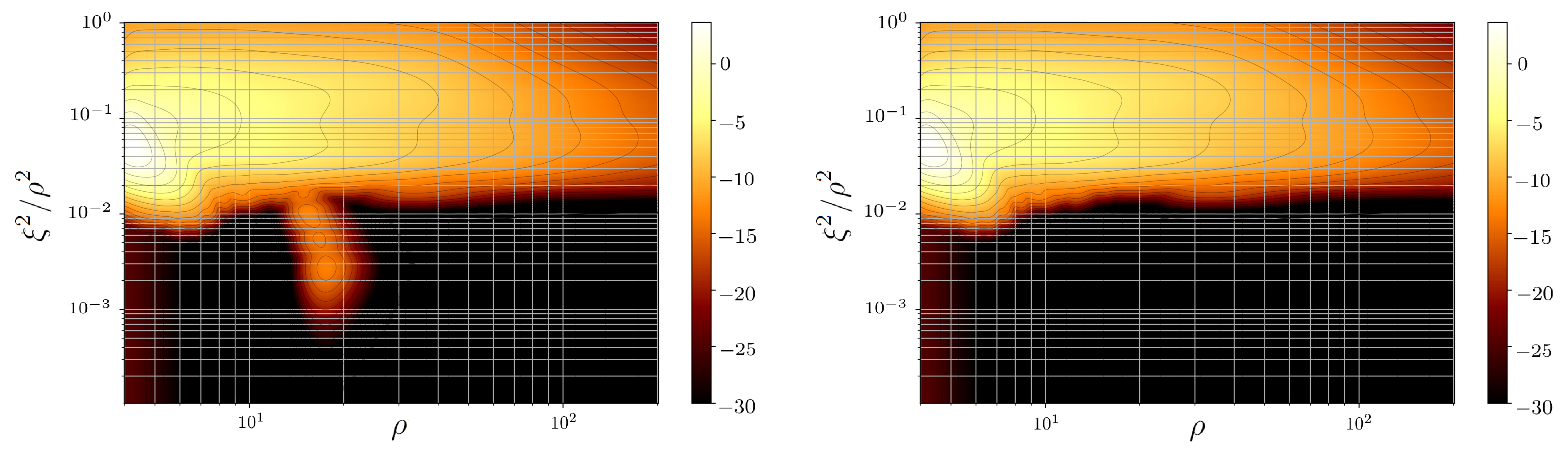
Figure 1: Left: An example of signal contamination in a $\rho-\xi^{2}$ PDF for Livingston. Right: The same PDF, with the contamination removed using the mechanism described in Sec. III.1. The color scheme encodes the probability density in a logarithmic scale with a brighter region having larger values. Note that kernel smoothing has been applied to these PDFs.

To prevent this, it is necessary to remove the events associated with such GW signals from the background histograms. However, there exists a tradeoff regarding which events one should choose to remove. Blindly removing all potential contamination risks undesirably eliminating actual noise events with high significance. Therefore, this contamination removal is designed to be a manual operation so that the user can decide the criterion by which to remove background events. For the GstLAL analysis, while the data is being analyzed and the histograms are being populated, we keep a temporary record of the non-coincident events from the last $5000\text{\,}\mathrm{s}$. If an event is above the open public alert significance threshold [41], it is considered as a potential contamination, and events within a $10\text{\,}\mathrm{s}$ window around the event of interest are permanently stored across all the template bins. Subsequently, these events are subtracted from the histograms so that the likelihood ratio can be evaluated without their contamination.

An example of the effect of signal contamination on a $\rho-\xi^{2}$ PDF, and the subsequent removal of the contamination are shown in Fig. 1. More information about the mechanism of removing signal contamination and its effect on the sensitivity of the GstLAL search can be found in [42].

III.2 Incorporation of bank $\xi^{2}$

Although SNR is known to be the optimal ranking statistic under Gaussian noise, nonstationary noise deviating from the Gaussian distribution, often referred to as glitches, can yield large SNR values and mimic a GW signal. Therefore, SNR alone does not characterize GW signals sufficiently. To deal with this, GstLAL adopts signal-based vetoes by introducing the $\xi^{2}$ parameter. Conceptually, these vetoes perform a consistency test between SNR values of a given event across a parameter space of our interest and its expected evolution in the presence of a signal. Up to the third observing run (O3), GstLAL calculated the $\xi^{2}_{\mathrm{a}}$ parameter by considering residual between SNR time series of a given event associated with a template $\alpha$ and its auto-correlation function. In what follows, we start with our conventional formalism of the $\xi^{2}_{\mathrm{a}}$ parameter and subsequently introduce an alternative $\xi^{2}$ parameters, which we call bank-$\xi^{2}$, developed for O4.

Given the two polarizations of GWs, we conventionally describe a template as complex values whose real and imaginary parts represent either $+$ or $\times$ polarization so that

$${h}_{\alpha}[\tau]={h}_{\alpha}^{+}[\tau]+i{h}_{\alpha}^{\times}[\tau].$$ (14)

With this representation of a template, we express the SNR timeseries associated with the template $\alpha$ as the following complex values

$$\hat{z}_{\alpha}[t]=\hat{z}_{\alpha}^{+}[t]+i\hat{z}_{\alpha}^{\times}[t].$$ (15)

Note that for the rest of this paper, we denote a hat symbol $\hat{x}$ to explicitly indicate $x$ is a random variable subject to noise fluctuation. The real and imaginary parts are the matched filter output for the template with either polarization, i.e.

$$\hat{z}_{\alpha}^{A}[t]=\sum_{\tau}{h}_{\alpha}^{A}[\tau]\hat{s}[t+\tau].$$ (16)

Here $\hat{s}[t]$ is whitened strain timeseries given from the upstream of a pipeline and ${h}_{\alpha}^{A}[\tau]$ is a whitened template normalized such that

$$\sum_{\tau}{h}_{\alpha}^{A}[\tau]{h}_{\alpha}^{A}[\tau]=1$$ (17)

for the two polarizations $A={\{+,\times\}}$.

Being analogous to the $\chi^{2}$ test in statistics, the $\hat{\xi}^{2}_{\mathrm{a}}$ parameter is defined as [16]

$$\hat{\xi}^{2}_{\mathrm{a}}=\frac{1}{N_{\mathrm{a}}}\sum_{t}\left|\hat{z}_{\alpha}[t]-\hat{z}_{\alpha}[0]R_{\alpha}[t]\right|^{2},$$ (18)

where $R_{\alpha}[t]$ is a complex auto-correlation function of the whitened template $\alpha$

$$R_{\alpha}[t]=\frac{1}{2}\sum_{\tau}{h}_{\alpha}[\tau]{h}_{\alpha}^{*}[t+\tau],$$ (19)

normalized as $R_{\alpha}[0]=1$. $N_{\mathrm{a}}$ is given by

$$N_{\mathrm{a}}=\sum_{t}\left\{2-2\left|R_{\alpha}[t]\right|^{2}\right\}$$ (20)

so that the expectation value of $\hat{\xi}^{2}_{\mathrm{a}}$ is unity, i.e. $\langle\hat{\xi}^{2}_{\mathrm{a}}\rangle=1$. Also, $t=0$ in Eq. (18) is chosen from the peak of $\left|\hat{z}_{\alpha}[t]\right|^{2}$, which is the best estimate of the merger time of a CBC signal. In practice, the summation over $\tau$ does not cover an infinite range, but rather one needs to select a finite auto-correlation length. For O4, we adopt the length of 701 (351) samples for templates with the chirp mass below (above) 15$M_{\odot}$, respectively. Note that in the case of the noiseless limit and a signal being identical to the associated template, the evolution of $\hat{z}_{\alpha}[t]$ follows the auto-correlation function with the proper scaling and phase shift accounted. Thus under Gaussian noise, the residual elements, $\hat{z}_{\alpha}[t]-\hat{z}_{\alpha}[0]R_{\alpha}[t]$, are each distributed as a Gaussian with zero mean and some correlation across samples at different timestamps. Given this property, the $\hat{\xi}^{2}_{\mathrm{a}}$ parameter allows us to assess the consistency of the SNR evolution over time by comparing the $\hat{\xi}^{2}_{\mathrm{a}}$ value against its expected distribution under the signal and noise models.

In general, $\xi^{2}$ parameters can be defined differently to perform a consistency test of SNR values in a parameter space other than time. Hence, we have developed bank-$\xi^{2}$ parameter [43], denoted as $\hat{\xi}^{2}_{\mathrm{b}}$, to explore the SNR evolution in template-bank space. Similarly to the conventional $\hat{\xi}^{2}_{\mathrm{a}}$ parameter shown in Eq. (18), we evaluate this statistic for an event associated with the template $\alpha$ by calculating the SNR residual across a group of templates denoted as $\{\bar{\theta}\}$:

$$\hat{\xi}^{2}_{\mathrm{b}}=\frac{1}{N_{\mathrm{b}}}\sum_{\beta\in\{\bar{\theta}\}}\left|\hat{z}_{\beta}[0]-\frac{1}{2}(h_{\beta}|h_{\alpha})\hat{z}_{\alpha}[0]\right|^{2},$$ (21)

where $(h_{\beta}|h_{\alpha})$ is the matched filter output between the two complex whitened templates, i.e.

$$(h_{\beta}|h_{\alpha})=\sum_{\tau}{h}_{\beta}[\tau]{h}_{\alpha}^{*}[\tau].$$ (22)

Here $N_{\mathrm{b}}$ is the normalization factor

$$N_{\mathrm{b}}=\sum_{\beta\in\{\bar{\theta}\}}\left\{2-\frac{1}{2}\left|(h_{\beta}|h_{\alpha})\right|^{2}\right\}$$ (23)

so that the expectation value of $\hat{\xi}_{\mathrm{b}}^{2}$ is unity, i.e. $\langle\hat{\xi}_{\mathrm{b}}^{2}\rangle=1$. Given the different parameter space which the $\hat{\xi}^{2}_{\mathrm{b}}$ parameter involves, its consistency test provides additional information about GW signals complementary to the $\hat{\xi}^{2}_{\mathrm{a}}$ parameter.

To take advantage of the benefits from both $\hat{\xi}^{2}_{\mathrm{a}}$ and $\hat{\xi}^{2}_{\mathrm{b}}$, we introduce a $\hat{\xi}^{2}_{\mathrm{ab}}$ parameter that combines the residual components of $\hat{\xi}^{2}_{\mathrm{a}}$ and $\hat{\xi}^{2}_{\mathrm{b}}$ as follows

$$\hat{\xi}^{2}_{\mathrm{ab}}=\frac{1}{N_{\mathrm{a}}+N_{\mathrm{b}}} \left(N_{\mathrm{a}}\hat{\xi}^{2}_{\mathrm{a}}+N_{\mathrm{b}}\hat{\xi}^{2}_{\mathrm{b}}\right)$$ (24)

$$\begin{split}=\frac{1}{N_{\mathrm{a}}+N_{\mathrm{b}}}&\left\{\sum_{t}\left|\hat{z}_{\alpha}[t]-\hat{z}_{\alpha}[0]R_{\alpha}[t]\right|^{2}\right.\\ &\left.+\sum_{\beta\in\{\bar{\theta}\}}\left|\hat{z}_{\beta}[0]-\frac{1}{2}(h_{\beta}|h_{\alpha})\hat{z}_{\alpha}[0]\right|^{2}\right\},\end{split}$$ (25)

where the normalization factor is applied similarly such that $\langle\hat{\xi}^{2}_{\mathrm{ab}}\rangle=1$. In Sec. IV, we show the sensitivity improvement of GstLAL pipeline due to this $\hat{\xi}^{2}_{\mathrm{ab}}$ parameter, using a simulated search for injected GW signals.

III.3 Upgraded $\rho-\xi^{2}$ signal model

Previously in O3, $P(\vec{\xi^{2}}\mid\vec{\rho},\theta,\mathcal{H}_{\mathrm{s}})$ in Eq. (2) followed an analytic function that was empirically obtained by tuning free parameters. Here, we describe a more accurate approximation of this PDF derived from the statistical properties of the $\xi^{2}$ parameter. In the rest of this subsection, we assume the signal hypothesis where a GW signal is present in Gaussian noise unless stated otherwise.

III.3.1 General formalism

We start with the general definition of the $\xi^{2}$ parameter:

$$\hat{\xi}^{2}=\frac{1}{N}\sum_{j}\left|\hat{z}_{j}-C_{ij}\hat{z}_{i}\right|^{2},$$ (26)

where $\hat{z}_{i}$ is a matched filter output at a reference point, denoted by the index $i$, of an arbitrary parameter and $N$ is a normalization factor, which reads

$$N=\sum_{j}\left\langle\left|\hat{z}_{j}-C_{ij}\hat{z}_{i}\right|^{2}\right\rangle.$$ (27)

$C_{ij}$ is a coefficient to construct expected morphology of $\{\hat{z}_{j}\}$, which can be thought of as a transfer function that relates $\hat{z}_{i}$ to $\hat{z}_{j}$, and this is given by $C_{ij}=\langle\hat{z}_{j}\hat{z}_{i}^{*}\rangle$ in the absence of a signal. Although $\xi^{2},N$ and quantities derived from these are specific to the reference point, indexed by $i$, of the parameter of interest, for brevity we do not explicitly indicate its dependence in these symbols.

Here, introducing a vector of the residual components

$$\vec{U}=\{\hat{U}_{j}\}=\hat{z}_{j}-C_{ij}\hat{z}_{i},$$ (28)

it follows that $\hat{\xi}^{2}\propto\vec{U}^{\dagger}\vec{U}$, where ^† represents Hermitian transpose of a given vector or matrix. Given the statistical properties of the matched filter output $\hat{z}_{i}$, $\vec{U}$ obeys a complex Gaussian distribution. In practice, there remains a systematic mismatch between the true signal and its associated template, leading to a non-zero mean of $\vec{U}$, which we denote as $\vec{\mu}=\langle\vec{U}\rangle$. Also, its covariance matrix is given by

$$\Sigma_{jk} =\langle(\hat{U}_{j}^{*}-\mu_{j}^{*})(\hat{U}_{k}-\mu_{k})\rangle$$ (29)

$$=C_{jk}-C_{ij}^{*}C_{ik}.$$ (30)

Consequently, one can find that

$$\vec{U}^{\dagger}\vec{U} =\sum_{j}\lambda_{j}|\hat{n}_{j}+\eta_{j}|^{2},$$ (31)

where $\{\lambda_{j}\}$ is an eigenvalue of the covariance matrix $\bm{\Sigma}$, $\{\hat{n}_{j}\}$ is normal random variables, and $\{\eta_{j}\}$ is the $j$-th component of $\vec{\mu}$ projected onto the eigenvector space of $\bm{\Sigma}$. See Appendix C for the derivation of Eq. (31).

The expression in RHS of Eq. (31) is known as generized chi-square distribution and there does not exist any closed-form expression of this PDF. However, this can be well approximated with a single chi-square distribution whose mean and variance are matched up with those derived from Eq. (31) [44], which yields

$$\langle\hat{\xi}^{2}\rangle =\frac{1}{N}\left\{\sum_{j}\lambda_{j}+\sum_{j}\lambda_{j}|\eta_{j}|^{2}\right\},$$ (32)

$$=\frac{1}{N}\left\{\mathrm{Tr}\bm{\Sigma}+\vec{\mu}^{\dagger}\vec{\mu}\right\},$$ (33)

$$\mathrm{Var}(\hat{\xi}^{2}) =\frac{2}{N^{2}}\left\{\sum_{j}\lambda_{j}^{2}+2\sum_{j}\lambda_{j}^{2}|\eta_{j}|^{2}\right\}.$$ (34)

$$=\frac{2}{N^{2}}\left\{\mathrm{Tr}\bm{\Sigma}^{2}+2\vec{\mu}^{\dagger}\bm{\Sigma}\vec{\mu}\right\}.$$ (35)

Given these known mean and variance, we parametrize the desired chi-square distribution with the following two parameters:

$$n_{\mathrm{eff}}=\frac{2\langle\hat{\xi}^{2}\rangle^{2}}{\mathrm{Var}(\hat{\xi}^{2})}$$ (36)

$$b=\frac{\mathrm{Var}(\hat{\xi}^{2})}{2\langle\hat{\xi}^{2}\rangle},$$ (37)

such that $\chi^{2}(x/b;n_{\mathrm{eff}})$ reproduces its mean and variance consistent with Eqs. (32) and (34), respectively. Therefore, we approximate that $P(\xi^{2}\mid\rho,\mathcal{H}_{\mathrm{s}})\approx\chi^{2}(\xi^{2}/b;n_{\mathrm{eff}})$. Note that this chi-square distribution depends on $\rho$ implicitly through $\{\eta_{j}\}$, which will be described in more details below in the case of the $\xi_{\mathrm{a}}^{2}$ parameter.

III.3.2 Application to $\hat{\xi}^{2}_{\mathrm{a}}$ parameter

We apply the above formalism to GstLAL’s conventional $\hat{\xi}^{2}_{\mathrm{a}}$ parameter based on its definition shown in Eq. (18). In this case, $i,j$ indices in Eq. (26) represent timestamps of SNR timeseries and specifically $t_{i}=0$. Also, from $C_{ij}=R[t_{j}-t_{i}]$ and Eq. (29), it follows that

$$\Sigma_{jk}=R[t_{k}-t_{j}]-R^{*}[t_{j}]R[t_{k}].$$ (38)

Regarding the mismatch between a true signal and its associated template, for simplicity we approximate it with the original auto-correlation function $R[t]$ overall scaled with the detected SNR and a fractional mismatch factor $k$, such that

$$\mu[t]=\langle\hat{z}[t]-\hat{z}[0]R[t]\rangle\approx k\rho R[t].$$ (39)

It is nontrivial to assess the accuracy of this approximation. Another possible approach would be to take the cross-correlation between a neighboring pair of templates. We leave the investigation of this and other avenues for improving the accuracy of this approximation to future work.

Nevertheless, Eq. (39) allows for rewriting Eqs. (32) and (34) in terms of $\vec{R}=\{R[t]\}$ as follows

$$\langle\hat{\xi}^{2}_{\mathrm{a}}\rangle =\frac{1}{N}\left\{\mathrm{Tr}\bm{\Sigma}+\rho^{2}k^{2}\vec{R}^{\dagger}\vec{R}\right\},$$ (40)

$$\mathrm{Var}(\hat{\xi}^{2}_{\mathrm{a}}) =\frac{2}{N^{2}}\left\{\mathrm{Tr}\bm{\Sigma}^{2}+2\rho^{2}k^{2}\vec{R}^{\dagger}\bm{\Sigma}\vec{R}\right\}.$$ (41)

This implies that, for given $\bm{\Sigma}$, $\rho$ and $k$, a single chi-square distribution $\chi^{2}(\xi^{2}/b;n_{\mathrm{eff}})$ is constructed based on Eqs. (36) and (37). Furthermore, this PDF is marginalized over a range of $k$, $0.1\text{\,}\mathrm{\char 37\relax}30\text{\,}\mathrm{\char 37\relax}$, as currently implemented in GstLAL. We iterate this process across different $\rho$ values until the $(\rho,\xi^{2})$ parameter space is sufficiently covered. See Fig. 5 for a visualization.

Eq. (18) shows that the $\hat{\xi}_{\mathrm{a}}^{2}$ parameter and its PDF are specific to the whitened auto-correlation function $R_{\alpha}[t]$ of a particular template $\alpha$, which in turn implicitly depends on a GW detector through whitening by its PSD. Also, as indicated by Eq. (7), for the sake of memory management we assign a common $P(\vec{\xi^{2}}\mid\vec{\rho},\theta,\mathcal{H}_{\mathrm{s}})$ PDF to a group of neighboring templates $\{\bar{\theta}\}$, which contains around 1000 templates in average, assuming that GW events associated with any of these templates follow the same signal model. To construct this representative PDF, the median of $\langle\hat{\xi}^{2}_{\mathrm{a}}\rangle$ and $\mathrm{Var}(\hat{\xi}^{2}_{\mathrm{a}})$ values are computed for each template group. The validity of this PDF depends on the similarity among the templates within each group, i.e. the efficiency of template grouping, whose details are described in [32]. As a result, we construct one $P\left(\xi^{2}_{\mathrm{d}}\mid\rho_{\mathrm{d}},\{\bar{\theta}\},\mathcal{H}_{\mathrm{s}}\right)$ signal model per template group per GW detector, and for a given detected event, $P(\vec{\xi^{2}}\mid\vec{\rho},\theta,\mathcal{H}_{\mathrm{s}})$ is evaluated in a multiplicative form with regard to participating GW detectors $\{\vec{O}\}$ as shown in Eq. (7).

III.4 KAGRA integration

KAGRA participated in the joint observation with GEO600 [45] detector at the end of O3 [46], and is planning to join the full GW detector network including Advanced LIGO and Virgo detectors during O4 [47]. Accordingly, GW detection pipelines need to incorporate the additional detector and conduct analysis across all the detectors in coincidence. With regard to GstLAL’s likelihood ratio, the two PDFs in the signal model, e.g. $P(\vec{O}\mid t_{\mathrm{ref}},\mathcal{H}_{\mathrm{s}})$ and $P(\Delta\vec{\ln\mathcal{D}},\vec{\Delta t},\vec{\Delta\phi}\mid\vec{O},t_{\mathrm{ref}},\mathcal{H}_{\mathrm{s}})$ are relevant to this integration. Here, we illustrate these PDFs in the presence of KAGRA and briefly discuss its characteristics.

Fig. 2 shows, as an example, the probability of only LIGO Hanford and KAGRA forming a coincident event while the two LIGO detectors and KAGRA operate, i.e. $P(\{H,K\}\mid t_{\mathrm{ref}},\mathcal{H}_{\mathrm{s}})$. This probability is evaluated as a function of horizon distances of KAGRA ($D_{K}$) and LIGO Livingston ($D_{L}$) relative to that of LIGO Hanford ($D_{H}$). Recall that $t_{\mathrm{ref}}$ is interchangeable with a vector of horizon distances, and hence taking different $t_{\mathrm{ref}}$ values is equivalent to exploring the two-dimensional parameter space $(D_{K}/D_{H},D_{L}/D_{H})$. The peak of the probability is located at $D_{K}/D_{H}\sim 1$ and $D_{L}/D_{H}\ll 1$, which is expected for both LIGO Hanford and KAGRA detectors to observe a signal and for LIGO Livingston detector to miss it. In practice, however, reasonable values of the fractional horizon distance among these detectors during O4 is far from the peak as indicated by the red marker in Fig. 2, implying heavy downranking if such an event is observed.

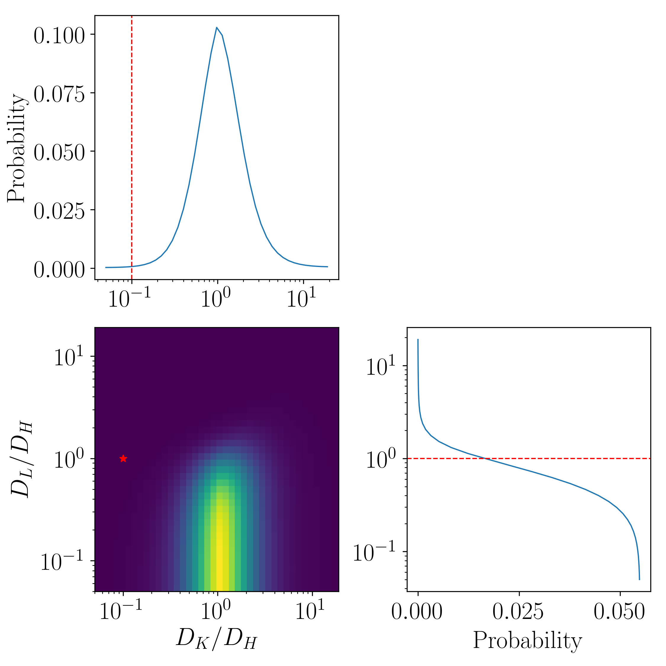
Figure 2: Example $P(\{H,K\}\mid t_{\mathrm{ref}},\mathcal{H}_{\mathrm{s}})$ while LIGO Hanford, Livingston and KAGRA operating, is evaluated as a function of fractional horizon distance between KAGRA ($D_{K}$) and LIGO Hanford ($D_{H}$) or between Hanford and Livingston ($D_{L}$), respectively. The color scheme in the two-dimensional plot encodes the probability density with a brighter region having larger values. The red marker indicates the reasonable values of the fractional horizon distance among these detectors during O4, being far from the peak.

In Fig. 3 we illustrate the two-dimensional PDF for the difference in GW arrival time and phase between LIGO Hanford and KAGRA, i.e. $P(\vec{\Delta{t}},\vec{\Delta{\phi}}\mid\{H,K\},t_{\mathrm{ref}},\mathcal{H}_{\mathrm{s}})$. Here we set the horizon distances of LIGO Hanford and KAGRA for a typical BNS source to be 410 Mpc and 6 Mpc, being consistent with the projected O4 PSD of the two detectors [47], and their representative SNRs to be 5 and 4, respectively. Therefore, Fig. 3 represents a slice of the three-dimensional PDF $P(\Delta\vec{\ln\mathcal{D}},\vec{\Delta t},\vec{\Delta\phi}\mid\vec{O},t_{\mathrm{ref}})$ where the effective distance ratio between the two detectors is given by their horizon distances and representative SNRs mentioned above. Also, we observe the characteristic structure in the marginalized $\Delta t$ distribution, $P(\Delta t\mid\{H,K\},t_{\mathrm{ref}},\mathcal{H}_{\mathrm{s}})$. This can be explained by the extreme value of the effective distance ratio between the two detectors, $\mathcal{D}_{H}/\mathcal{D}_{K}=16.5$, which allows only a narrow range of extrinstic parameters to contribute to the PDF. In particular, such a limited range of sky position is manifested by the noticeable structure in $P(\Delta t\mid\{H,K\},t_{\mathrm{ref}},\mathcal{H}_{\mathrm{s}})$.

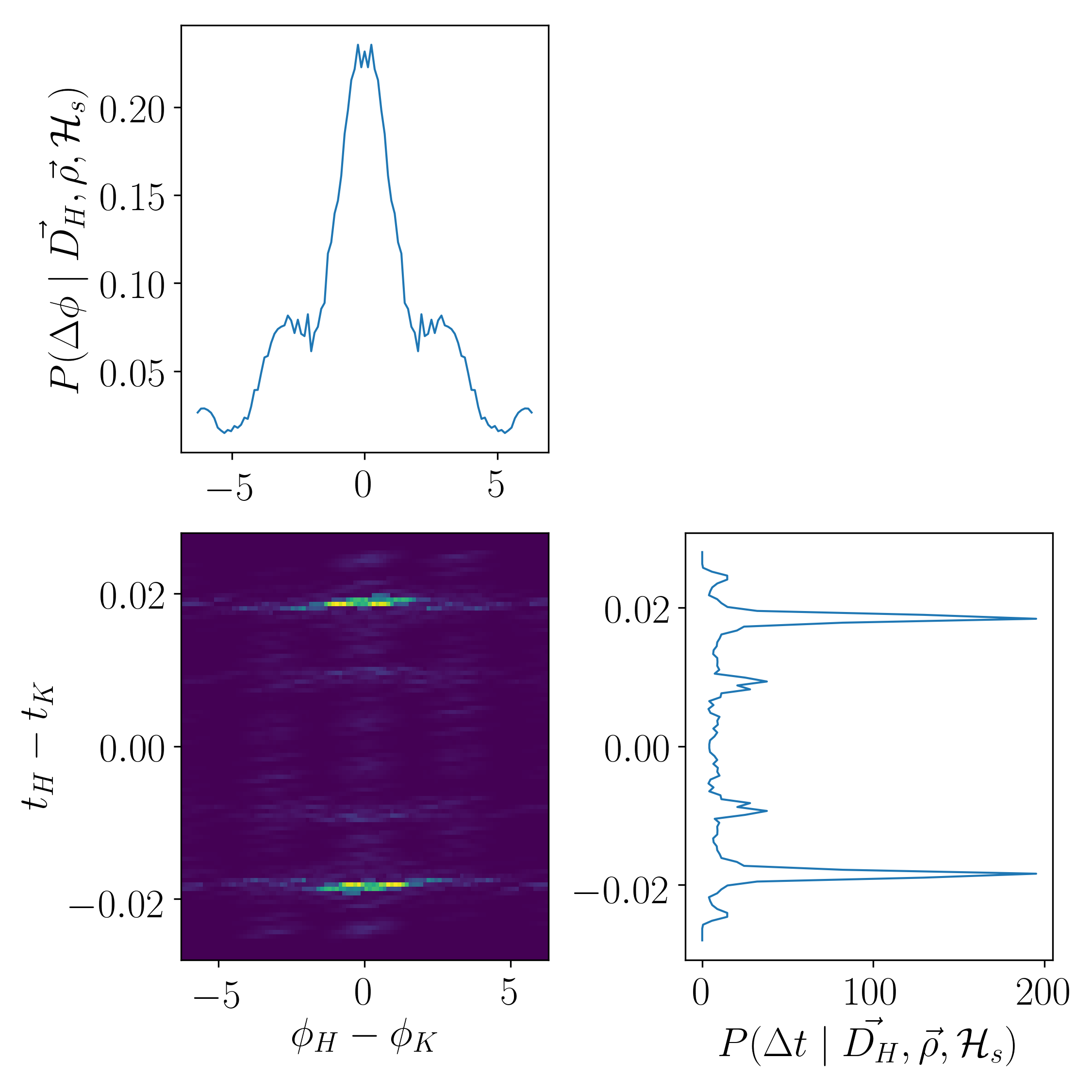
Figure 3: Example $P(\vec{\Delta{t}},\vec{\Delta{\phi}}\mid\{H,K\},t_{\mathrm{ref}},\mathcal{H}_{\mathrm{s}})$ and its marginalized PDF for LIGO Hanford and KAGRA. The color scheme in the two-dimensional plot encodes the probability with a brighter region having larger values. Here we set the horizon distances of LIGO Hanford and KAGRA to be 410 Mpc and 6 Mpc respectively to be consistent with the projected O4 PSD of the two detectors [47], and show a slice of the three-dimensional PDF where the ratio of the effective distance between the two detectors is somewhat reasonable given their horizon distances.

IV Results

IV.1 Sensitive space-time volume

We conduct an injection study using GstLAL with the new features described in Sec. III and discuss the improvement in the pipeline’s sensitivity, focusing on the bank-$\xi^{2}$ incorporation and the upgraded $\rho-\xi^{2}$ signal model. For each injection run, to quantify the sensitivity we measure the sensitive space-time volume ($VT$) as a function of false alarm rate (FAR), which is defined as

$$VT(\mathrm{FAR})=T\int_{0}^{\infty}\epsilon(z,\mathrm{FAR})\frac{dV_{c}(z)}{dz}\frac{1}{1+z}\,\mathrm{d}z,$$ (42)

where $T$ is the duration of a simulated observation, $\epsilon(z,\mathrm{FAR})$ is the detection efficiency for the GW signals which are injected at the redshift in [$z,z+\mathrm{d}z$] and recovered at FAR below a given threshold, and $V_{c}(z)$ is the comoving volume at the redshift of $z$. Note that $VT$ depends on the source distribution of injected GW signals, and in what follows, we apply the same injection set between two runs for valid $VT$ comparison.

IV.2 Incorporation of bank $\xi^{2}$

For a simulated observation, we analyze the O3 dataset between 18 April 2019 16:46 UTC and 26 April 2019 17:14 UTC with 86606 synthetic CBC signals injected. This injection set contains signals from BNSs whose component masses ($m_{1},m_{2}$) go up to $3M_{\odot}$, BBHs whose $m_{1},m_{2}$ go up to $50M_{\odot}$, and intermediate-mass black holes whose $m_{1},m_{2}$ go up to $300M_{\odot}$. For this study, we use the template bank used for O3 [4], which covers the entire set of injections.

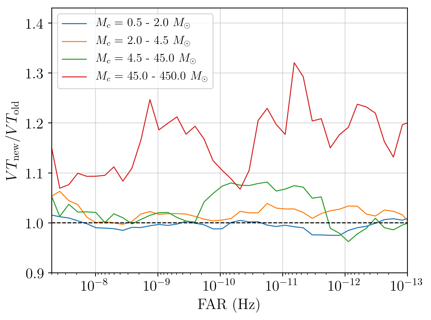
Figure 4: Ratio of the $VT$ value measured by the run with the combined $\xi^{2}$ to that with the normal $\xi^{2}_{\mathrm{a}}$ as a function of FAR, and hence the value above 1 indicates the sensitivity improvement due to the incorporation of bank $\xi^{2}$ statistics. The different colors represent the four chirp-mass ($M_{c}$) bins mentioned in the legend.

Given the injection set, we conduct two sets of the simulated observations with the conventional $\xi_{\mathrm{a}}^{2}$ and the combined $\xi^{2}_{\mathrm{ab}}$ statistics defined in Eq. (25), respectively, and measure the $VT$ value for each of the two cases. When evaluating the $VT$ values, we bin the entire set of injections into four chirp-mass ($M_{c}$) ranges: $0.5\text{\,}2.0\text{\,}$$\ M_{\odot}$(BNS), $2.0\text{\,}4.5\text{\,}$$\ M_{\odot}$(lighter BBH), $4.5\text{\,}45\text{\,}$$\ M_{\odot}$(heavier BBH) and $45\text{\,}450\text{\,}$$\ M_{\odot}$(IMBH). Fig. 4 is a ratio of the $VT$ value measured by the run with the combined $\xi^{2}_{\mathrm{ab}}$ to that with the $\xi^{2}_{\mathrm{a}}$ as a function of FAR, and hence the values above 1 indicates the sensitivity improvement due to the incorporation of bank-$\xi^{2}$ statistics. The different colors represent the four chirp-mass bins mentioned above.

One can find that at the FAR of $3.2\text{\times}{10}^{-8}\text{\,}\mathrm{Hz}$($\approx 1$ per year) the $VT$ ratio increases by $10\text{\,}\mathrm{\char 37\relax}$ (or even more at lower FAR) for IMBH injections, while the other three categories do not exhibit noticeable improvement. This difference can be understood by the duration of those injected signals in the detector’s frequency band. Given the shortest duration of IMBH signals, the time-domain consistency test performed by the $\xi^{2}_{\mathrm{a}}$ statistic do not help those signals to be distinguished from noise, and hence the complimentary test on the template domain using the $\xi^{2}_{\mathrm{ab}}$ statistic is rather informative, leading to the significant improvement in the $VT$ value as shown in Fig. 4. Note that the zig-zaggy structure in IMBH’s $VT$ ratio is due to relatively large uncertainty in each $VT$ measurement given a smaller number of recovered IMBH injections than other source categories.

IV.3 Upgraded $\rho-\xi^{2}$ signal model

We analyze the same dataset and injection set described in Sec. IV.2. Yet, we use the template bank developed for O4, adopting the manifold placement algorithm [49] and the sorting scheme using the orthogonalized PN-phase terms described in [32, 50]. Fig. 5 shows a scatter plot of recovered BNS injections, represented by blue circles, on top of the $P(\xi^{2}_{H}\mid\rho_{H},\{\bar{\theta}\},\mathcal{H}_{\mathrm{s}})$ PDF associated with one of the BNS template groups for LIGO Hanford detector. This visually demonstrates that the density of recovered BNS injections on $(\rho,\xi^{2})$ parameter space is largely consistent with the upgraded signal model, verifying the validity of the derivation described in Sec. III.3.

Given the injection set, we conduct two sets of the simulated observations with and without the upgraded $\rho-\xi^{2}$ signal model, respectively, and measure the $VT$ value for each of the two cases. Binning the injection set in the same way as Sec. IV.2, Fig. 6 shows a ratio of the $VT$ value measured by the run with the upgraded signal model to that with the original signal model as a function of FAR. This figure implies that at the FAR of $3.2\text{\times}{10}^{-8}\text{\,}\mathrm{Hz}$($\approx 1$ per year) the $VT$ ratio increases by $15\text{\,}\mathrm{\char 37\relax}$ ($20\text{\,}\mathrm{\char 37\relax}$) for BNS (lighter BBH) injections, while the heavier BBH and IMBH injections do not exhibit noticeable improvement. Since BNS and lighter BBH signals produce longer duration, the time-domain consistency test by $\xi^{2}_{\mathrm{a}}$ statistics tend to be more impactful for these source categories than heavier ones.

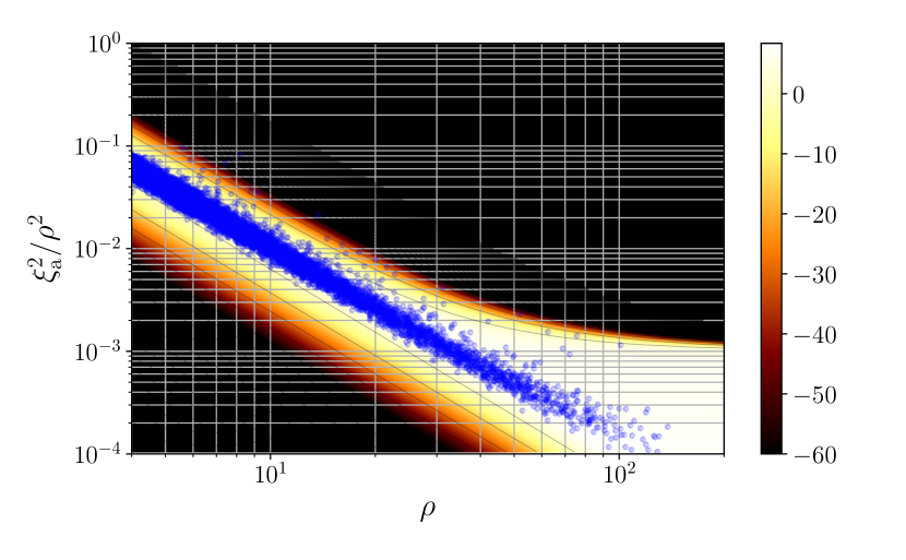
Figure 5: Scatter plot of recovered BNS injections, denoted by blue circles, on top of the $P(\xi^{2}_{H}\mid\rho_{H},\{\bar{\theta}\},\mathcal{H}_{\mathrm{s}})$ associated with BNS templates for LIGO Hanford detector. The color scheme encodes the probability density in a logarithmic scale with a brighter region having larger values.

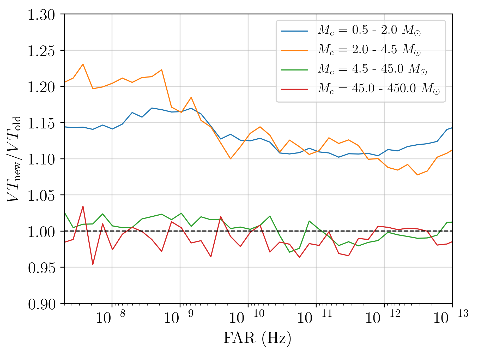
Figure 6: Ratio of the $VT$ value measured by the run with the upgraded signal model to that with the original signal model as a function of FAR, and hence the values above 1 indicates the sensitivity improvement due to the upgraded signal model. The different colors represent the four chirp-mass ($M_{c}$) bins mentioned in the legend.

V Conclusion

In this work we have described several new features implemented in GstLAL-based insprial pipeline, leading up to O4. These features consist of: the signal contamination removal, the bank-$\xi^{2}$ incorporation, the upgraded $\rho-\xi^{2}$ signal model and the integration of KAGRA. Specifically, we have demonstrated by the $VT$ comparison that the bank-$\xi^{2}$ incorporation improves the sensitivity to IMBH signals by $10\text{\,}\mathrm{\char 37\relax}$ or more and that the upgraded $\rho-\xi^{2}$ signal model improves the sensitivity to BNS (lighter BBH) signals by $15\text{\,}\mathrm{\char 37\relax}$ ($20\text{\,}\mathrm{\char 37\relax}$), respectively. Although we have not quantitatively shown the performance of the signal contamination removal, Fig. 1 visually illustrates that the signal contamination can be fully removed. A more thorough investigation using blind injections is described in [42]. Also, in the injection study shown in Sec. IV, we did not incorporate the upgraded $\rho-\xi^{2}$ signal model and the bank-$\xi^{2}$ statistic both simultaneously for one configuration, which requires derivation and recalculation of the covariance matrix shown in Eq. (38). We leave this as future work to address during offline reanalysis of O4 dataset. Regarding the overall performance of the latest GstLAL analysis, see [40] for the detailed results of the Mock Data Challenge conducted as preparation of O4.

Appendix A Derivation of Eq. (6)

We start with the following coordinate transformation shown in Eq. (4):

$$\vec{\rho}\rightarrow\vec{x}=\left(\begin{array}[]{c}\rho_{\mathrm{net}}\\ \ln\left\{\mathcal{D}_{2}/\mathcal{D}_{\mathrm{ref}}\right\}\\ \vdots\\ \ln\left\{\mathcal{D}_{n}/\mathcal{D}_{\mathrm{ref}}\right\}\end{array}\right).$$ (47)

In general, any coordinate transformation in the probability density involves modification in the volume element characterized by Jacobian matrix, which explicitly reads

$$\bm{\mathcal{J}}(\vec{\rho})=\begin{pmatrix}\frac{\partial x_{1}}{\partial\rho_{1}}&\cdots&\frac{\partial x_{i}}{\partial\rho_{1}}&\cdots&\frac{\partial x_{n}}{\partial\rho_{1}}\\ \vdots&\ddots&&&\vdots\\ \frac{\partial x_{1}}{\partial\rho_{j}}&&\frac{\partial x_{i}}{\partial\rho_{j}}&&\frac{\partial x_{n}}{\partial\rho_{j}}\\ \vdots&&&\ddots&\vdots\\ \frac{\partial x_{1}}{\partial\rho_{n}}&\cdots&\frac{\partial x_{i}}{\partial\rho_{n}}&\cdots&\frac{\partial x_{n}}{\partial\rho_{n}}\end{pmatrix}.$$ (48)

Note that in this particular case the new coordinates, $\vec{x}$, can be written in terms of the original SNR coordinates such that

$$x_{1}=\rho_{\mathrm{net}},\qquad x_{i}=\ln\left\{\frac{D_{i}}{D_{1}}\right\}-\ln\left\{\frac{\rho_{i}}{\rho_{1}}\right\},$$ (49)

where $D_{i}$ is the horizon distance for $i$-th detector.

For example, when evaluating Eq. (5) for coincident triggers between LIGO Hanford and Livingston detectors, the SNR coordinates are given by

$$\rho_{1}=\rho_{H},\qquad\rho_{2}=\rho_{L}.$$ (50)

Hence, the Jacobian matrix Eq. (48) takes the form of

$$\bm{\mathcal{J}}(\rho_{H},\rho_{L})=\begin{pmatrix}\frac{\rho_{H}}{\sqrt{\rho_{H}^{2}+\rho_{L}^{2}}}&&\frac{\rho_{L}}{\sqrt{\rho_{H}^{2}+\rho_{L}^{2}}}\\ &&\\ \frac{1}{\rho_{H}}&&-\frac{1}{\rho_{L}}\\ \end{pmatrix},$$ (51)

which leads to the determinant

$$|\bm{\mathcal{J}}(\vec{\rho})|=\frac{\sqrt{\rho_{H}^{2}+\rho_{L}^{2}}}{\rho_{H}\rho_{L}}.$$ (52)

Similarly, this derivation can be extended to the three-detector case, and in general, one finds the general expression of the determinant shown in Eq. (6).

Appendix B Derivation of Eq. (9)

The probability of observing $k$ noise events with the mean rate $\mu$ during unit observation time $T$ follows a Poisson distribution

$$P(N=k\mid\mu)=\frac{1}{k!}(\mu T)^{k}\mathrm{e}^{-\mu T}.$$ (53)

In GstLAL’s implementation, the total event rate consists of several categories characterized by a template group $\{\bar{\theta}\}$, i.e. $\mu=\sum_{\{\bar{\theta}\}}\mu_{\{\bar{\theta}\}}$, and Eq. (53) is assumed to hold independently for noise events from each category. Since $P\left(t_{\mathrm{ref}},\theta\mid\mathcal{H}_{\mathrm{n}}\right)$ considers a situation where the given event occurs for the associated template group and no others, the PDF reads

$$P\left(t_{\mathrm{ref}},\theta\mid\mathcal{H}_{\mathrm{n}}\right) =P(1\mid\mu_{\{\bar{\theta}\}})\prod_{i\neq\{\bar{\theta}\}}P(0\mid\mu_{i})$$ (54)

$$=\mu_{\{\bar{\theta}\}}T\mathrm{e}^{-\mu T}.$$ (55)

Since the exponential factor is constant across different template groups, the only dependence on $\theta$ boils down to $\mu_{\{\bar{\theta}\}}$ as shown in Eq. (9).

Appendix C Derivation of Eq. (31)

From the definition of $\bm{\Sigma}$ shown in Eq. (29), one can find that $\bm{\Sigma}$ is positive semidefinite, and hence, there exists square root of $\bm{\Sigma}$ such that $\bm{A}^{2}=\bm{\Sigma}$. Introducing $\vec{V}=\bm{A}^{-1}\vec{U}$, from $\vec{U}\sim\mathcal{N}(\vec{\mu},\bm{\Sigma})$, it follows that $\vec{V}\sim\mathcal{N}(\bm{A}^{-1}\vec{\mu},\mathbbm{1})$. Furthermore, since $\bm{\Sigma}$ can be diagonalized as $\bm{\Sigma}=\bm{P}^{\dagger}\bm{\Lambda}\bm{P}$, where $\bm{P}$ is a unitary transformation matrix and $\bm{\Lambda}$ is a diagonal matrix with entries $\lambda_{i}$, Eq. (31) reads

$$\vec{U}^{\dagger}\vec{U} =\vec{V}^{\dagger}(\bm{A}^{2})\vec{V}=\vec{V}^{\dagger}(\bm{P}^{\dagger}\bm{\Lambda}\bm{P})\vec{V}$$ (56)

$$=\vec{W}^{\dagger}\bm{\Lambda}\vec{W}=\sum_{i}\lambda_{i}|\hat{n}_{i}+\eta_{i}|^{2}.$$ (57)

Here Eq. (57) is given by the fact that $\vec{W}=\bm{P}\vec{V}\sim\mathcal{N}(\vec{\eta},\mathbbm{1})$, where $\vec{\eta}=\bm{A}^{-1}\vec{\mu}$. This also implies that $|\hat{n}_{i}+\eta_{i}|^{2}$ obeys noncentral chi-square distribution with the 2 degrees of freedom and noncentral parameter of $|\eta_{i}|^{2}$. Therefore, this formalism suggests that $\vec{U}^{\dagger}\vec{U}$, or equivalently the $\xi^{2}$ parameter, is a weighted sum (characterized by $\lambda_{i}$) of multiple chi-square random variables, which is in general referred to as generalized chi-square distribution. See [51] for more detailed discussion.

References

- Abbott et al. [2019] B. Abbott, R. Abbott, T. Abbott, S. Abraham, F. Acernese, K. Ackley, C. Adams, R. Adhikari, V. Adya, C. Affeldt, et al., Gwtc-1: a gravitational-wave transient catalog of compact binary mergers observed by ligo and virgo during the first and second observing runs, Physical Review X 9, 031040 (2019).
- gwt [2021] Gwtc-2: Compact binary coalescences observed by ligo and virgo during the first half of the third observing run, Physical Review X 11, 021053 (2021).
- The LIGO Scientific Collaboration et al. [2021a] The LIGO Scientific Collaboration, The Virgo Collaboration, R. Abbott, et al., Gwtc-2.1: Deep extended catalog of compact binary coalescences observed by ligo and virgo during the first half of the third observing run (2021a).
- The LIGO Scientific Collaboration et al. [2021b] The LIGO Scientific Collaboration, The Virgo Collaboration, The KAGRA Collaboration, R. Abbott, et al., Gwtc-3: Compact binary coalescences observed by ligo and virgo during the second part of the third observing run (2021b).
- Aasi et al. [2015] J. Aasi et al. (LIGO Scientific), Advanced LIGO, Class. Quant. Grav. 32, 074001 (2015), arXiv:1411.4547 [gr-qc] .
- Acernese et al. [2015] F. Acernese et al. (VIRGO), Advanced Virgo: a second-generation interferometric gravitational wave detector, Class. Quant. Grav. 32, 024001 (2015), arXiv:1408.3978 [gr-qc] .
- Abbott et al. [2017a] B. P. Abbott et al., GW170817: Observation of Gravitational Waves from a Binary Neutron Star Inspiral, Physical Review Letters 119, 161101 (2017a), arXiv:1710.05832 [gr-qc] .
- Abbott et al. [2017b] B. P. Abbott et al. (LIGO Scientific Collaboration and Virgo Collaboration), Multi-messenger Observations of a Binary Neutron Star Merger, Astrophys. J. Lett. 848, L12 (2017b), arXiv:1710.05833 [astro-ph.HE] .
- [9] https://gcn.gsfc.nasa.gov/other/G298048.gcn3.
- 170 [2018] Gw170817: Measurements of neutron star radii and equation of state, Physical Review Letters 121, 10.1103/PhysRevLett.121.161101 (2018).
- Abbott et al. [2017a] B. P. Abbott et al., Estimating the contribution of dynamical ejecta in the kilonova associated with GW170817, The Astrophysical Journal 850, L39 (2017a).
- 170 [2019] Properties of the binary neutron star merger gw170817, Physical Review X 9, 10.1103/PhysRevX.9.011001 (2019).
- Abbott et al. [2017b] B. P. Abbott et al., On the progenitor of binary neutron star merger GW170817, The Astrophysical Journal 850, L40 (2017b).
- [14] Igwn public alerts user guide:observing capabilities, https://emfollow.docs.ligo.org/userguide/capabilities.html.
- Akutsu et al. [2020] T. Akutsu et al., Overview of KAGRA: Detector design and construction history, Progress of Theoretical and Experimental Physics 2021, 10.1093/ptep/ptaa125 (2020), 05A101, https://academic.oup.com/ptep/article-pdf/2021/5/05A101/37974994/ptaa125.pdf .
- Messick et al. [2017] C. Messick, K. Blackburn, P. Brady, P. Brockill, K. Cannon, R. Cariou, S. Caudill, S. J. Chamberlin, J. D. Creighton, R. Everett, C. Hanna, D. Keppel, R. N. Lang, T. G. Li, D. Meacher, A. Nielsen, C. Pankow, S. Privitera, H. Qi, S. Sachdev, L. Sadeghian, L. Singer, E. G. Thomas, L. Wade, M. Wade, A. Weinstein, and K. Wiesner, Analysis framework for the prompt discovery of compact binary mergers in gravitational-wave data, Physical Review D 95, 10.1103/PhysRevD.95.042001 (2017).
- Sachdev et al. [2019] S. Sachdev, S. Caudill, H. Fong, R. K. L. Lo, C. Messick, D. Mukherjee, R. Magee, L. Tsukada, K. Blackburn, P. Brady, P. Brockill, K. Cannon, S. J. Chamberlin, D. Chatterjee, J. D. E. Creighton, P. Godwin, A. Gupta, C. Hanna, S. Kapadia, R. N. Lang, T. G. F. Li, D. Meacher, A. Pace, S. Privitera, L. Sadeghian, L. Wade, M. Wade, A. Weinstein, and S. L. Xiao, The gstlal search analysis methods for compact binary mergers in advanced ligo’s second and advanced virgo’s first observing runs (2019), arXiv:1901.08580 [gr-qc] .
- Hanna et al. [2020] C. Hanna, S. Caudill, C. Messick, A. Reza, S. Sachdev, L. Tsukada, K. Cannon, K. Blackburn, J. D. E. Creighton, H. Fong, P. Godwin, S. Kapadia, T. G. F. Li, R. Magee, D. Meacher, D. Mukherjee, A. Pace, S. Privitera, R. K. L. Lo, and L. Wade, Fast evaluation of multidetector consistency for real-time gravitational wave searches, Phys. Rev. D 101, 022003 (2020).
- LIGO Scientific Collaboration and Virgo Collaboration [2023] LIGO Scientific Collaboration and Virgo Collaboration, Gstlal, git.ligo.org/lscsoft/gstlal (2023).
- [20] Gstreamer, https://gstreamer.freedesktop.org/documentation/index.html.
- LIGO Scientific Collaboration [2018] LIGO Scientific Collaboration, LIGO Algorithm Library - LALSuite, free software (GPL) (2018).
- Wainstein et al. [1970] L. Wainstein, V. D. Zubakov, and A. A. Mullin, Extraction of signals from noise (1970).
- Hawking and Israel [1989] S. W. Hawking and W. Israel, Three Hundred Years of Gravitation (1989).
- Sathyaprakash [1991] B. S. Sathyaprakash, Choice of filters for the detection of gravitational waves from coalescing binaries, Physical Review D 44, 3819 (1991).
- Cutler et al. [1993] C. Cutler, T. A. Apostolatos, L. Bildsten, L. S. Finn, E. E. Flanagan, D. Kennefick, D. M. Markovic, A. Ori, E. Poisson, G. J. Sussman, and K. S. Thorne, The last three minutes: Issues in gravitational-wave measurements of coalescing compact binaries, Phys. Rev. Lett. 70, 2984 (1993).
- Finn [1992] L. S. Finn, Detection, measurement, and gravitational radiation, Physical Review D 46, 5236 (1992).
- Finn [1993] L. S. Finn, Observing binary inspiral in gravitational radiation: One interferometer, Physical Review D 47, 2198 (1993).
- Dhurandhar and Sathyaprakash [1994] S. V. Dhurandhar and B. S. Sathyaprakash, Choice of filters for the detection of gravitational waves from coalescing binaries. ii. detection in colored noise, Phys. Rev. D 49, 1707 (1994).
- Balasubramanian [1996] R. Balasubramanian, Gravitational waves from coalescing binaries: Detection strategies and monte carlo estimation of parameters, Physical Review D 53, 3033 (1996).
- Flanagan and Hughes [1998] E. E. Flanagan and S. A. Hughes, Measuring gravitational waves from binary black hole coalescences. i. signal to noise for inspiral, merger, and ringdown, Phys. Rev. D 57, 4535 (1998).
- Mukherjee et al. [2021] D. Mukherjee, S. Caudill, R. Magee, C. Messick, S. Privitera, S. Sachdev, K. Blackburn, P. Brady, P. Brockill, K. Cannon, S. J. Chamberlin, D. Chatterjee, J. D. E. Creighton, H. Fong, P. Godwin, C. Hanna, S. Kapadia, R. N. Lang, T. G. F. Li, R. K. L. Lo, D. Meacher, A. Pace, L. Sadeghian, L. Tsukada, L. Wade, M. Wade, A. Weinstein, and L. Xiao, Template bank for spinning compact binary mergers in the second observation run of advanced ligo and the first observation run of advanced virgo, Phys. Rev. D 103, 084047 (2021).
- Sakon et al. [2022] S. Sakon, L. Tsukada, H. Fong, C. Hanna, J. Kennington, S. Adhicary, K. Cannon, S. Caudill, B. Cousins, J. D. E. Creighton, B. Ewing, P. Godwin, Y.-J. Huang, R. Huxford, P. Joshi, R. Magee, C. Messick, S. Morisaki, D. Mukherjee, W. Niu, A. Pace, C. Posnansky, S. Sachdev, D. Singh, R. Tapia, D. Tsuna, T. Tsutsui, K. Ueno, A. Viets, L. Wade, M. Wade, and J. Wang, Template bank for compact binary mergers in the fourth observing run of advanced ligo, advanced virgo, and kagra (2022).
- Nitz [2018] A. H. Nitz, Rapid detection of gravitational waves from compact binary mergers with pycbc live, Physical Review D 98, 10.1103/PhysRevD.98.024050 (2018).
- Aubin et al. [2021] F. Aubin, F. Brighenti, R. Chierici, D. Estevez, G. Greco, G. M. Guidi, V. Juste, F. Marion, B. Mours, E. Nitoglia, O. Sauter, and V. Sordini, The MBTA pipeline for detecting compact binary coalescences in the third LIGO–virgo observing run, Classical and Quantum Gravity 38, 095004 (2021).
- Chu [2022] Q. Chu, Spiir online coherent pipeline to search for gravitational waves from compact binary coalescences, Physical Review D 105, 10.1103/PhysRevD.105.024023 (2022).
- Cannon et al. [2015] K. Cannon, C. Hanna, and J. Peoples, Likelihood-ratio ranking statistic for compact binary coalescence candidates with rate estimation (2015).
- Neyman et al. [1933] J. Neyman, E. S. Pearson, and K. Pearson, Ix. on the problem of the most efficient tests of statistical hypotheses, Philosophical Transactions of the Royal Society of London. Series A, Containing Papers of a Mathematical or Physical Character 231, 289 (1933), https://royalsocietypublishing.org/doi/pdf/10.1098/rsta.1933.0009 .
- Fong [2018] H. Fong, From simulations to signals: Analyzing gravitational waves from compact binary coalescences, Ph.D. thesis, University of Toronto (2018).
- Schutz [2011] B. F. Schutz, Networks of gravitational wave detectors and three figures of merit, Classical and Quantum Gravity 28, 125023 (2011).
- Ewing et al. [2023] B. Ewing, R. Huxford, D. Singh, L. Tsukada, C. Hanna, Y.-J. Huang, P. Joshi, A. K. Y. Li, R. Magee, C. Messick, A. Pace, A. Ray, S. Sachdev, S. Sakon, R. Tapia, S. Adhicary, P. Baral, A. Baylor, K. Cannon, S. Caudill, S. S. Chaudhary, M. W. Coughlin, B. Cousins, J. D. E. Creighton, R. Essick, H. Fong, R. N. George, P. Godwin, R. Harada, J. Kennington, S. Kuwahara, D. Meacher, S. Morisaki, D. Mukherjee, W. Niu, C. Posnansky, A. Toivonen, T. Tsutsui, K. Ueno, A. Viets, L. Wade, M. Wade, and G. Waratkar, Performance of the low-latency gstlal inspiral search towards ligo, virgo, and kagra’s fourth observing run (2023), arXiv:2305.05625 [gr-qc] .
- [41] Igwn public alerts user guide, https://emfollow.docs.ligo.org/userguide/analysis/index.html##alert-threshold.
- Joshi et al. [2023] P. Joshi et al., Background filter: A method for removing signal contamination during significance estimation of a gstlal anaysis, (in prep) (2023).
- Hanna [2008] C. Hanna, SEARCHING FOR GRAVITATIONAL WAVES FROM BINARY SYSTEMS IN NON-STATIONARY DATA, Ph.D. thesis, Louisiana State University (2008).
- Tn et al. [1968] N. Tn, N. At, A. H. Feiveson, and F. C. Delaney, THE DISTRIBUTION a N D PROPERTIES OF a WEIGHTED SUM OF CHI SQUARES (1968).
- Dooley et al. [2016] K. L. Dooley, J. R. Leong, T. Adams, C. Affeldt, A. Bisht, C. Bogan, J. Degallaix, C. Gräf, S. Hild, J. Hough, A. Khalaidovski, N. Lastzka, J. Lough, H. Lück, D. Macleod, L. Nuttall, M. Prijatelj, R. Schnabel, E. Schreiber, J. Slutsky, B. Sorazu, K. A. Strain, and H. Vahlbruch, GEO 600 and the GEO-HF upgrade program: successes and challenges, Classical and Quantum Gravity 33, 075009 (2016).
- Collaboration et al. [2022] T. L. S. Collaboration, T. V. Collaboration, T. K. Collaboration, R. Abbott, et al., First joint observation by the underground gravitational-wave detector KAGRA with GEO 600, Progress of Theoretical and Experimental Physics 2022, 10.1093/ptep/ptac073 (2022), 063F01, https://academic.oup.com/ptep/article-pdf/2022/6/063F01/43989382/ptac073.pdf .
- Abbott et al. [2020] B. P. Abbott et al., Prospects for observing and localizing gravitational-wave transients with advanced ligo, advanced virgo and kagra, Living Reviews in Relativity 23, 3 (2020).
- Allen et al. [2012] B. Allen, W. G. Anderson, P. R. Brady, D. A. Brown, and J. D. E. Creighton, Findchirp: An algorithm for detection of gravitational waves from inspiraling compact binaries, Phys. Rev. D 85, 122006 (2012).
- Hanna et al. [2022] C. Hanna et al., A binary tree approach to template placement for searches for gravitational waves from compact binary mergers (2022), arXiv:2209.11298 [gr-qc] .
- Morisaki [2020] S. Morisaki, Rapid parameter estimation of gravitational waves from binary neutron star coalescence using focused reduced order quadrature, Physical Review D 102, 10.1103/PhysRevD.102.104020 (2020).
- Mathai and Provost [1992] A. Mathai and S. Provost, Quadratic Forms in Random Variables, Statistics: A Series of Textbooks and Monographs (Taylor & Francis, 1992).