Unpacking merger jets: a Bayesian analysis of GW170817, GW190425
and electromagnetic observations of short gamma-ray bursts
Abstract
We present a novel fully Bayesian analysis to constrain short gamma-ray burst jet structures associated with cocoon, wide-angle and simple top-hat jet models, as well as the binary neutron star merger rate. These constraints are made given the distance and inclination information from GW170817, observed flux of GRB 170817A, observed rate of short gamma-ray bursts detected by Swift, and the neutron star merger rate inferred from LIGO’s first and second observing runs. A separate analysis is conducted where a fitted short gamma-ray burst luminosity function is included to provide further constraints. The jet structure models are further constrained using the observation of GW190425 and we find that the assumption that it produced a GRB 170817-like short gamma-ray burst that went undetected due to the jet geometry is consistent with previous observations. We find and quantify evidence for low luminosity and wide-angled jet structuring in the short gamma-ray burst population, independently from afterglow observations, with log Bayes factors of for such models when compared to a classical top-hat jet. Slight evidence is found for a Gaussian jet structure model over all others when the fitted luminosity function is provided, producing log Bayes factors of when compared to the other models. However without considering GW190425 or the fitted luminosity function, the evidence favours a cocoon-like model with log Bayes factors of over the Gaussian jet structure. We provide new constraints to the binary neutron star merger rates of Gpc-3 yr-1 or Gpc-3 yr-1 when a fitted luminosity function is assumed.
1 Introduction
The joint detection of both gravitational wave (GW) GW170817 (Abbott et al., 2017a), and counterpart short gamma-ray burst (sGRB) GRB 170817A (Goldstein et al., 2017; Savchenko et al., 2017), followed by the detection of kilonova AT 2017gfo (McCully et al., 2017; Evans et al., 2017) not only solidified the belief that sGRBs are produced from the merger of binary neutron star (BNS) systems, but also began the era of GW multimessenger astronomy (Abbott et al., 2017a). The combination of both the and GW data gave insight into various problems that a detection through a single data channel could not provide; ranging from cosmology (Abbott et al., 2017b), the origin of the abundance of heavy elements in the universe (Tanvir et al., 2017), tests of general relativity and the speed of gravity (Abbott et al., 2017c) among others.
However the detection of the event not only provided answers but also provoked questions, as it was inferred through GW parameter inference that the event was exceptionally nearby at only Mpc (Abbott et al., 2019), giving an observed isotropic luminosity of the event of erg s-1, three orders of magnitude lower than that observed for any other sGRB (Abbott et al., 2017c). It was also inferred through GW parameter inference that the event was viewed at a wide angle of from the central axis (Abbott et al., 2019). This lead to the hypothesis that the jet of GRB 170817A exhibited some wide-angle structure to produce the observed flux, and that it may still have had a typically luminous central jet component. The long duration observations of the event’s afterglow across the electromagnetic (EM) spectrum provided further evidence for this claim (Troja et al., 2017; Margutti et al., 2018; Lyman et al., 2018; D’Avanzo et al., 2018; Mooley et al., 2018; Ruan et al., 2018; Troja et al., 2018; Alexander et al., 2018; Troja et al., 2020).
While evidence for this wide-angled structure is provided by the multitude of afterglow observations, the functional form of the luminosity profile over viewing angle remains in question (e.g. Granot et al., 2017; Duffell et al., 2018; Gottlieb et al., 2018; Lamb & Kobayashi, 2018; Mooley et al., 2018; Troja et al., 2018; Ioka & Nakamura, 2019; Beniamini et al., 2019; Fraija et al., 2019; Lamb et al., 2019; Salafia et al., 2019; Biscoveanu et al., 2020; Lamb et al., 2020; Takahashi & Ioka, 2021). Accurate modelling of this jet structure is important in both understanding the astrophysics of the event, and in preventing systematic biases in any multimessenger analysis that must make assumptions about the jet geometry (Nakar & Piran, 2021; Lamb et al., 2021), which include constraints on the Hubble constant (Abbott et al., 2017b) and the BNS merger rate (Wanderman & Piran, 2015).
With the promise of future GW BNS merger detections (Abbott et al., 2020b), a jet structure model that best represents the data of joint detection events should be discerned (Hayes et al., 2020). However, current analyses are limited to the data provided by GW170817/GRB 170817A (including AT 2017gfo), GW BNS merger event GW190425 (Abbott et al., 2020a), as well as the population of sGRBs detected independently of GW detection (Poolakkil et al., 2021; Lien et al., 2016). Previous similar work has considered constraining jet structure models with joint GW and EM detections using a Bayesian analysis (Biscoveanu et al., 2020; Hayes et al., 2020; Farah et al., 2020). The historical rate of detected sGRB and GWs has also been used in Bayesian analyses to constrain the jet structure (Williams et al., 2018; Sarin et al., 2022). Work by Mogushi et al. (2019) and Tan & Yu (2020) combine the detection rates of sGRB and GWs with the prompt emission data of GRB 170817A and the parameter inference results of GW170817, along with assuming a luminosity function fitted by short gamma-ray burst events with known redshift. The jet structure has been constrained given the weak gamma-ray emission detected by the INTEGRAL detector coincident with the gravitational wave event GW190425 in the work by Saleem et al. (2020). In this work, we put forward a comprehensive Bayesian framework that combines the prompt emission data from GRB 170817A, GW parameter inference posteriors of GW170817 and GW190425, GW informed BNS merger rate, as well as the detection rate of sGRBs by the Neil Gehrels Swift Observatory (Swift) detector. This analysis is then further combined with the information provided by a luminosity function fitted by sGRB events with known redshifts to provide tighter constraints, with the caveat of also introducing bias into the analysis. We provide parameter constraints and model comparison results between a classical top-hat jet structure and three different jet structures with wide-angled structuring: a Gaussian, power-law and double Gaussian jet. These results are presented alongside constraints on the intrinsic luminosity (when it is not fitted by the luminosity function), and the merger rate for both cases.
The physical model assumed is detailed in Section 2, before the analysis method and data are laid out in Section 3. In Section 4 we report the results of the analysis, both for when the fitted luminosity function is incorporated and when it is not. In Section 5 the implications of the results are discussed and a conclusion provided in Section 6.
2 Background
The sGRB data consists of the observed T90 integrated flux as well as the number of observed sGRBs . The average T90 integrated flux is related to the isotropic equivalent luminosity at a given viewing angle , as well as a redshift dependent luminosity distance and -correction :
| (1) |
The mean number of sGRBs observed by a detector within a duration that covers an area of sky equal to depends on the redshift, viewing angle and intrinsic luminosity through the number density:
| (2) |
where denotes the selection effects of the detector, such that if a detection is made and otherwise.
We consider sGRBs detected by the Swift instrument, which has a detector response determined empirically in (Lien et al., 2014) to fit:
| (3) |
where , , , , erg s-1 cm-2 and erg s-1 cm-2.
The relation between the number density and the physical parameters of is:
| (4) |
where is the co-moving volume, is the rate of sGRBs and is the intrinsic luminosity function given the hyperparameter .
2.1 Short gamma-ray burst rate
The rate of sGRBs is assumed to be in the form:
| (5) |
where is the local rate of BNS mergers and is defined so that . This assumes that every BNS merger results in a sGRB, and that the number of sGRBs produced by neutron star-black hole mergers is negligible.
The form of can be assumed to follow the star formation rate convolved with the probability distribution of the delay time between the system formation and the eventual merger that leads to the sGRB (Wanderman & Piran, 2015):
| (6) |
where is the redshift when the system was formed, is the look-back time and is the minimum delay time. This minimum delay time is set to Myr and according to (Guetta & Piran, 2006). The star formation rate is assumed to be of the form (Cole et al., 2001):
| (7) |
where the parameter values are taken from (Hopkins & Beacom, 2006) to be , , and .
2.2 Cosmology
A flat, vacuum dominated universe is assumed. The co-moving volume distribution over redshift is defined:
| (8) |
For a flat cosmology, the luminosity distance is related to the redshift by:
| (9) |
where is the Hubble constant and is equal to:
| (10) |
Here and are the matter density and dark energy density respectively (Hogg, 1999), with values taken from (Adam et al., 2016) along with km s-1 Mpc-1.
The look-back time, defined as the time between when a source emits light at redshift and the time it is detected, is then:
| (11) |
For a flat, vacuum dominated universe, the inverse function has an analytical expression (Petrillo et al., 2013):
| (12) |
where:
| (13) |
2.3 Intrinsic and isotropic equivalent luminosity
The luminosity structure of a gamma-ray burst is defined to be:
| (15) |
where is the intrinsic luminosity at . It is assumed that the distribution of intrinsic luminosity follows a Schechter function:
| (16) |
for where and .
Similarly the Lorentz factor’s dependence over angle follows:
| (17) |
with being the Lorentz factor of the jet at . Given these definitions, both and are defined to equal 1 at .
The Lorentz factor determines the degree of relativistic beaming, which for the luminosity is governed by:
| (18) | ||||
with and where .
The apparent isotropic equivalent luminosity, for an observer at from the jet axis, can then be related to the intrinsic luminosity via the beaming function by combining Eqn. 15 and Eqn. 18:
| (19) |
where is the maximum angle for which the beaming of gamma-rays occurs. A conservative maximum outer jet angle for the emission of gamma-rays is approximated by considering scattering by electrons accompanying baryons within the jet. The condition is given by (Matsumoto et al., 2019; Lamb et al., 2022),
| (20) |
Beyond this limit, , the jet becomes opaque to gamma-rays.
2.4 Jet structures
The implications of structuring within compact stellar merger jets for the EM counterparts from GW detected systems has been highlighted in the literature (Lamb & Kobayashi, 2017; Lazzati et al., 2017; Kathirgamaraju et al., 2018; Beniamini et al., 2020); here we choose a sample of fiducial jet structure models that are representative of the literature diversity.
The top-hat jet (TH) is the simplest structure, where the beam is uniform until the jet opening angle where the jet sharply cuts off:
| (21) | ||||
We note that the condition expressed in Eqn. 20 is not enforced for this case, as is above the Eqn. 20 limit at all points within the jet.
Wide-angle structure can be introduced with a Gaussian jet (GJ) structure, described by a single width parameter (e.g. Rossi et al., 2002, 2004; Zhang & Meszaros, 2002; Kumar & Granot, 2003):
| (22) |
An alternative to the Gaussian profile has the wide-angle emission expressed as a three parameter power-law jet (PL) structure (e.g. Kumar & Granot, 2003; Zhang et al., 2004; Rossi et al., 2004), where the jet can be described by some uniform core out to width , and then the intrinsic luminosity structure falls off at wide angles according to power and the Lorentz factor with :
| (23) | ||||
Finally, let us consider a two component, or double Gaussian jet (DG), with emission from both an inner core described by a Gaussian structure of width and an outer cocoon described by width (Salafia et al., 2020):
| (24) | |||
The luminosity of the outer cocoon is equal to and the Lorentz factor .
We do not consider hollow-cone jet structure models in our study (see e.g., Nathanail et al., 2021; Takahashi & Ioka, 2021); we expect that the combination of our intrinsic luminosity distribution (Eqn. 16) and the beaming (Eqn. 19) will wash-out the effect of any hollow-cone structuring within the core. For this study, the structure outside of the jet’s core is the critical component.
3 Bayesian framework
Constraints are placed on model parameters of a model when given data in Bayesian data analysis by determining the posterior distribution using Bayes theorem:
| (25) |
where is the likelihood, is the prior and the normalisation term is the evidence. Consider comparing two models and when given data . In the context of Bayesian data analysis, the statistic used to compare two models is the posterior odds defined:
| (26) |
Normally we are interested in cases where the a priori probability of either model being correct is comparable, and therefore the posterior odds is dominated by the Bayes factor:
| (27) |
which quantifies the contribution to the posterior odds given by the data . A value of favours , while favours .
The analysis is performed by applying the model described in Section 2 with an assumed jet structure from Section 2.4 given both GW and sGRB prompt emission data.
Table 1 lists the notation used in the following section. The data can be split into that produced by a GW-triggered event, denoted with the subscript ‘GW’, and that produced from an EM trigger, denoted with the subscript ‘EM’.
The data from the GW-triggered events consists of the GW strain and the flux of the counterpart . The GW-triggered events may not necessarily require a counterpart to be considered for the analysis. If the sky localisation of the source coincides with the sky coverage of gamma-ray burst detectors then we can assume that it was not detected due to its distance and orientation to us. The current events that meet this criteria are both GW170817 with GRB 170817A as well as GW190425 and the non-detection of its counterpart, under the assumption that a sGRB was produced, given the Fermi detector covered of the sky localisation and Konus–Wind covered the entire sky (Hosseinzadeh et al., 2019).
The EM-triggered events are simply the number of sGRB detections that Swift made within a 10 year operational period .
| Variable | Description |
| GW detector data | |
| sGRB detector data | |
| Number of detected GWs | |
| Number of detected sGRBs | |
| Luminosity function hyperparameters | |
| BNS merger rate | |
| Jet structure parameters | |
| Intrinsic on-axis luminosity |
| Data set | Data |
The likelihood can be decoupled into two terms, one of which considers GW-triggered events and the other EM-triggered:
| (28) |
The likelihood of the EM-triggered events is a Poisson distribution with a mean given in Eqn. 2:
| (29) |
The mean is evaluated over a regular grid of shape .The angular grid points were chosen to be distributed over a power-law so as to populate low areas of the parameter space with grid points, while also maintaining a relatively high density of points at wider angles where emission from some jet structures is still significant.
The GW-triggered events likelihood is the product of each of the events:
| (30) |
where samples are taken of and from . The parameters can be sampled from separate distributions and respectively, where are samples from the posteriors produced from GW parameter estimation for each event. The likelihood of the prompt emission of the GW-triggered events is assumed to be a Gaussian distribution of width about a mean described in Eqn. 1:
| (31) |
The priors for the model are specified in Table 3 for each of the gamma-ray burst rate, luminosity function and jet structure parameters. A normal distribution is denoted with a mean of and standard deviation of , a uniform distribution as with lower bound of and upper bound of , a Gamma distribution and inverse Gamma distribution as and with a shape of and a scale of . We assume that every BNS merger results in a gamma-ray burst so that .
| Model | Parameter | Prior |
| ′ | ||
| TH | ||
| GJ | ||
| PL | ||
| DG | ||
The T90 integrated flux of GRB 170817A in the Fermi detector’s keV band is set at erg s-1 cm-2 with an uncertainty of erg s-1 cm-2 (Goldstein et al., 2017). For the unobserved counterpart of GW190425, it is assumed that the T90 integrated flux takes a value of zero with an uncertainty of erg s-1 cm-2 as a conservative upper bound to the Fermi detector’s detection threshold (Tan & Yu, 2020). The distance and viewing angle posteriors of GW170817 and GW190425 are each represented by samples taken from the their respective parameter estimation data releases. In this work we consider an observing period of approximately years by the Swift detector in which it observed sGRBs as recorded by Lien et al. (2016), given a sky coverage of . The log prior on the rate of BNS mergers of is roughly chosen to reflect the constraints imposed to the rates by GWTC-2 (Abbott et al., 2020c). The log prior on is centred around the fitted value taken from Mogushi et al. (2019) with a standard deviation set to span one order of magnitude. This is chosen to reflect some prior information in the allowed luminosity from prior observations, but with a width to allow for flexibility into higher or lower luminosity regimes.
Posteriors and Bayes factors are calculated from Eqn. 25 and Eqn. 27 by assigning and as the variables in Table 1. We collect the data into three sets: one only given the number of Swift detections and GW detections called , another with the combined GW170817 GW and EM data called , and the other with GW190425 GW data and the flux from the non-detection called . The analysis is performed on five combinations of these data sets: , , , , and . We allow that , where are the jet structure model parameters dependent on jet structure model . The three analyses are repeated for each of the jet structure models: TH, GJ, PL and DG.
The posterior samples and evidence for each case are calculated via the nested sampling algorithm Nessai, that utilises machine learning techniques to drastically reduce the number of evaluations of the expensive likelihood function (Williams et al., 2021).
4 Results
| Top-hat | Gaussian | Power-law | Double Gaussian | |
| Top-hat | ||||
| Gaussian | ||||
| Power-law | ||||
| Double Gaussian |
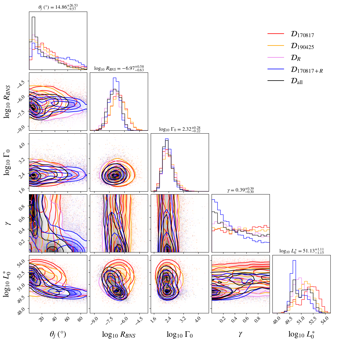
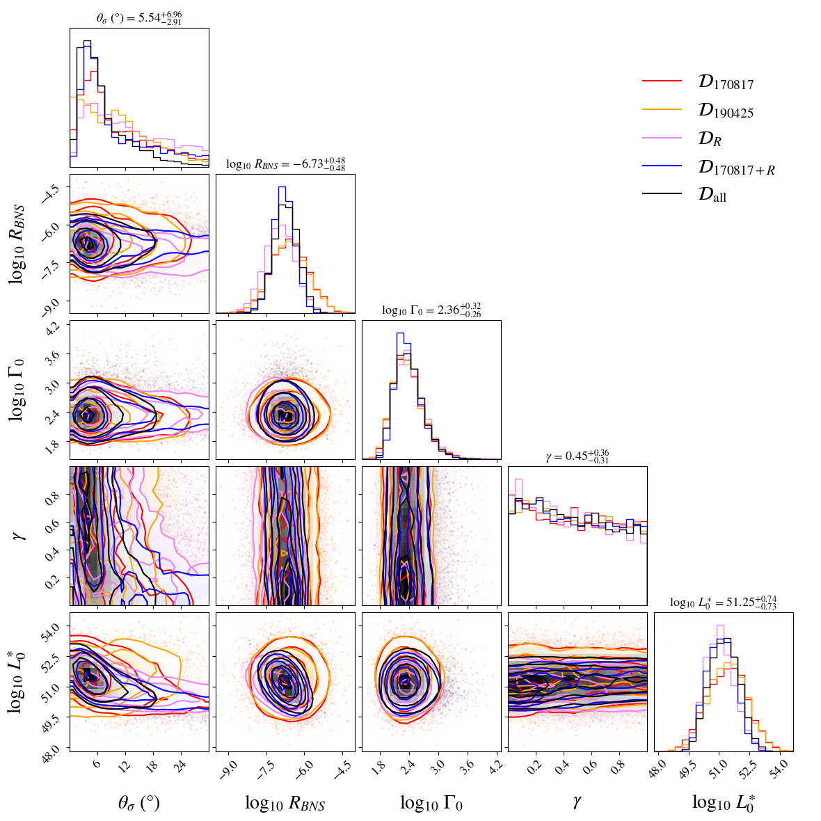
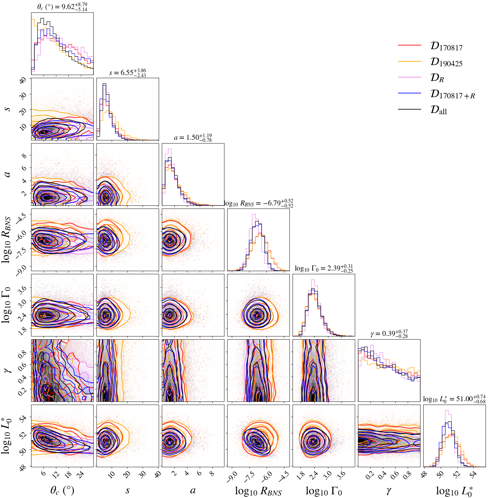
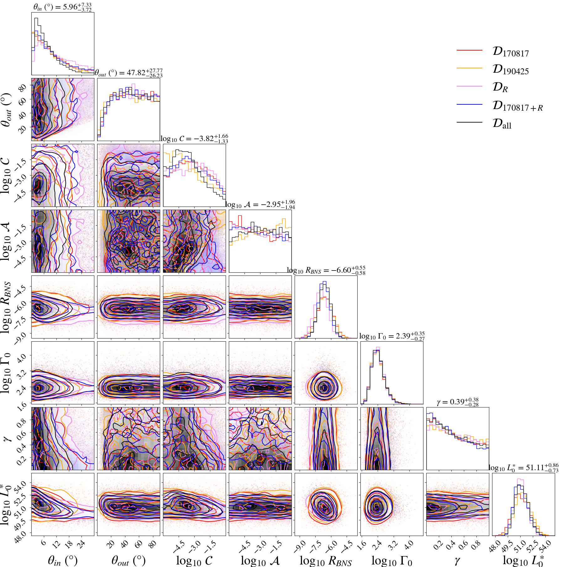
The analysis that is described in the previous section is applied to all three sets of data. The full corner plots for each jet structure model are shown in the appendix, where Figure A1 shows the results for the top-hat jet, Figure A2 the Gaussian jet, Figure A3 the power-law jet and Figure A4 the double Gaussian jet structure model. The posteriors for each of the data sets is overlaid upon one another where is shown in red, in orange, in violet, in blue and in black. The log evidence that corresponds to each posterior is shown in Table A1 for each of the five data sets over the four jet structure models. The log Bayes factors between the different models given the same data set can simply be calculated by taking the difference between entries of the same row.
Much of the discussion in this section concerns the posterior constraints when all of the data is considered , however the outcomes given the other subsets are considered to explain these results and provide further insight.
The log Bayes factors between the jet structure models are given as the left-hand entries of Table 4 when given the data. A positive value indicates that the data supports the model of the row while a negative value supports the column model. Evidently the top-hat model is less favourable than the models with wide-angled jet structuring, with Bayes factors of , and between it and the Gaussian, power-law and Double Gaussian jet structures respectively. The log Bayes factors between the power-law, Gaussian and the double Gaussian is slight, with only insignificant evidence in favour of the Gaussian and double Gaussian model of log Bayes factors of less than , and negligibly small log Bayes factors between the two.
The constraints on the rate of BNS mergers when given are shown in Figure LABEL:fig:BNSrate for the four jet structure models. These constraints take the form of posterior distributions that are represented in the violin plots, where the outermost solid vertical lines indicate the minimum and maximum sample value while the fill in between represents the probability density. The narrowest credible intervals are shown by the vertical dashed lines which enclose the median indicated by the middle solid line. The posterior distributions are compared to samples from the prior distribution at the top of the figure. For all cases, the posterior places tighter constraints on the merger rate than the prior distribution. The cases with wide-angled structuring (Gaussian, power-law and double Gaussian models) produce similar posterior distributions to one another, centred around a value of Mpcyr-1 consistent with the mean of the prior. The Gaussian jet structure produces the narrowest constraints with a credible interval of , compared to the power-law and double Gaussian models of and respectively. The top-hat model favours lower rates of BNS mergers, and even pushes the lower bound on the credible interval to lower values of that of the prior, constraining it between .
The median intrinsic luminosity posteriors determined for each model when given is shown in Figure LABEL:fig:L0. The mean intrinsic luminosity is determined by drawing and from the respective posterior distribution and then drawing samples from the corresponding Schechter function of Eqn. 16 before finding the ensemble median. This process is then repeated for median intrinsic luminosity samples. These posteriors take a form similar to the rates posteriors in Figure LABEL:fig:BNSrate as violin plots where the shaded probability density is contained within the outermost maximum and minimum values indicated by the solid vertical lines, while the median is marked by the middle solid line. The median is enclosed by the narrowest credible intervals displayed as dashed vertical lines. A distribution of prior samples of is also plotted at the top of the figure, which is determined by sampling from the individual and priors defined in Table 3. The top-hat jet structure resembles the prior in width, but shifts to favour lower luminosity and exhibits some bimodality as the probability density pinches at the median. This is due to the bimodality of the posterior distribution in Figure A1 given , which shall be discussed later in Section 5. The models with wide-angled structure tend towards lower mean intrinsic luminosity values, with the Gaussian model constrained to , power-law model and double Gaussian model of . The top-hat model is constrained to which we can compare to the prior of .
| Model | Parameter | Constraints | |
| w/o fitted LF | Fitted LF | ||
| TH | |||
| GJ | |||
| PL | |||
| DG | |||
The constraints from the posteriors on the jet structure parameters given each jet structure model are shown in Table 5. The median is quoted along with the upper and lower bounds placed by the narrowest credible intervals.
4.1 Fitted luminosity function
The analysis is repeated but instead of assuming a prior distribution on the luminosity scale and shape, a luminosity function fitted from the observed isotropic equivalent luminosity of sGRBs with associated redshifts. The values of and are taken from the mean fitted Schechter function in Mogushi et al. (2019) of and , fitted to the isotropic equivalent luminosity of sGRBs.
The log evidence between each of the jet structure models and the different data sets are shown in Table A2, while the respective Bayes factors when given between each of the jet structure models are shown on the right-hand entries of Table 4.
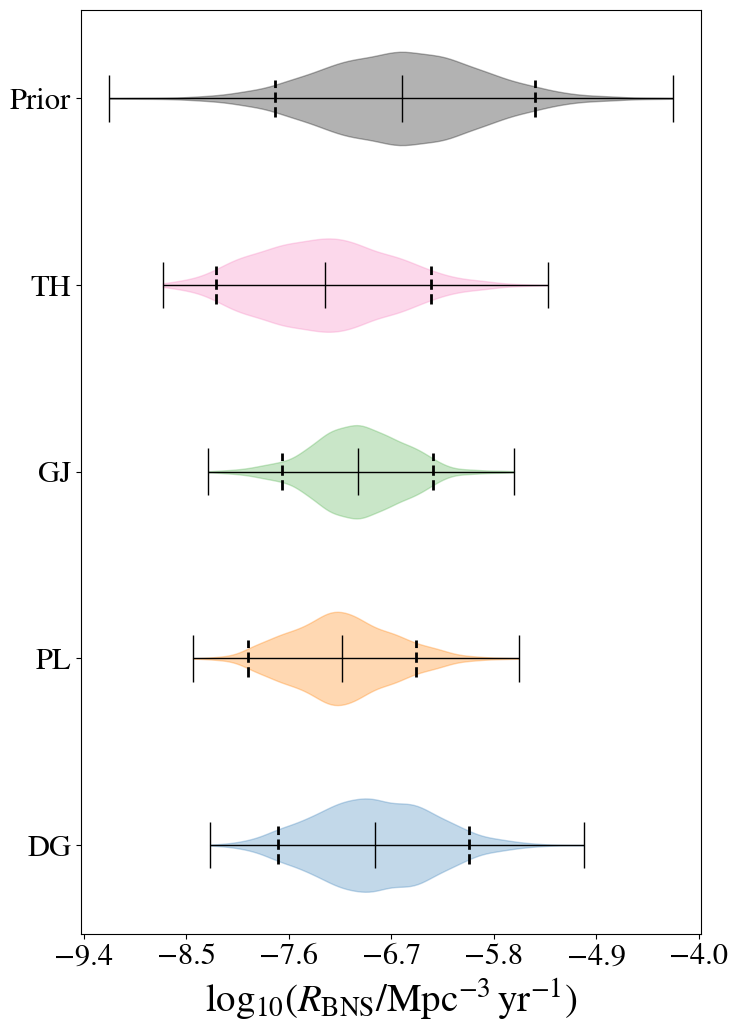
The posteriors on the local rate of BNS merger when given the fitted luminosity function and are shown in Figure 3 in the same format as Figure LABEL:fig:BNSrate, where the widths of the violin plots indicate the probability density, the maximum and minimum sample is indicated by the extreme solid vertical lines, and median with the middle solid vertical line. The narrowest credible intervals are indicated by the dashed vertical lines and are , , for the Gaussian, power-law and double Gaussian models respectively. For the top-hat jet model, the rate is constrained to .
The constraints on the jet structure models when given the fitted luminosity function and are presented in Table 5 for each jet structure models, with the upper and lower bounds representing the narrowest credible intervals.
5 Discussion
5.1 Wide-angle jet structuring
The log Bayes factors are greater than for all models with wide-angle jet structure when compared to the top-hat model. This is due to the top-hat jets failing to resolve the number of observed sGRBs with the flux of GRB 170817A when assuming that the event had a typical event opening angle. Given the assumed star formation rate and the constraints on the BNS merger rate from gravitational-wave detections, to obtain a Swift sGRB detection rate of yr-1, the jets are either predicted to have narrow opening angles and high luminosities or wide opening angles and low luminosities. This constraint can be seen in the bottom left corner plot panel of Figure A1 in the violet posterior, where much of the probability density is concentrated in the low luminosity and wide opening angle area of the parameter space. In contrast, the constraints made by GW170817 and GRB 170817A favour a wide opening angle of and a high luminosity event, as seen in the bottom left-hand panel of Figure A1 in the red posterior. This is as emission from an event from a top-hat jet structure when viewed at wide angles can only come from Doppler beaming, which falls off very sharply with increased viewing angles. As is more probable than , then a high luminosity event is deemed more probable. The two constraints produce posteriors that share very little overlap in the parameter space, leading to the top-hat model providing a smaller evidence than the other models. This contradiction also manifests in the bimodality of the mean luminosity posterior for the top-hat jet model, as seen in Figure LABEL:fig:L0, as the lower luminosity high density region corresponds to the constraint produced from the observed number of gamma-ray bursts, while the higher luminosity high density region corresponds to the constraints made by GW170817 and GRB 170817A.
Jet structure models with wide-angle structuring are only favoured when the data from GW170817/GRB 170817A of is combined with the event rate information from . When these data sets are considered individually the evidence for a top-hat jet structure is comparable or higher than the other models in most cases, as seen in the Table A1. The inclusion of the GW190425 event provides evidence against jets with wide-angle structuring. This can be seen by comparing the difference in log evidence between the top-hat jet and the other models given , and the difference when given , where there is relatively less evidence between the models when is included. As it is assumed that GW190425 produced a counterpart that went undetected due to its distance and viewing angle, the event places an upper-bound on the luminosity and jet width. This upper bound on the jet structure limits the possible wide-angle emission, which makes wide-angle jet structuring unnecessary to explain the event.
5.2 Cocoon emission
The double Gaussian jet structure provides a stand-in for a jet structure with cocoon-like emission, where the outer Gaussian provides a secondary component for the emission contribution from an energetic cocoon. Interestingly, comparing the log evidence given the double Gaussian jet model to the other models shows weak evidence for the double Gaussian jet structure when considering , , for all cases (with the exception of given the fitted Schechter luminosity function), suggesting it is the favourable model when considering both GW170817/GRB 170817A and the observed rate data. As discussed in the previous section, GW190425 places an upper-bound on the wide-angled emission and provides support for the top-hat and power-law jet structure with sharper cut-offs. Given that the suitability of GW190425 in the analysis is not as clear-cut as an event like GW170817 due to the uncertainty of the EM coverage of the event, this result should not be disregarded. While this may not provide convincing evidence for the observation of cocoon emission, it suggests that with the inclusion of future events, the necessity for the cocoon-like component can be better assessed.
5.3 Rate of binary neutron star mergers
The narrowest credible intervals of the rate of BNS mergers are constrained within Gpc-3 yr-1 independent of the jet structure model considered, improving upon the constraints imposed by GWTC-3 (Abbott et al., 2023). The rate is further constrained to the interval of Gpc-3 yr-1 when the fitted Schechter luminosity function is assumed. Future BNS detections will provide tighter constraints on their merger rate. These constraints will allow for a tighter prior to be placed on the rate of mergers, allowing the possible jet structures to be distinguished.
5.4 Luminosity function
Two different cases are explored in the analysis: one where the luminosity function is fitted in advance of the analysis, and the other where priors are placed on the luminosity function parameters and . When priors are placed on the luminosity function, the luminosity function generally favours low luminosities for all models assumed. This is apparent in Figure LABEL:fig:L0 where the posterior for all jet structure models shifts to low luminosity when compared to the prior distribution, and mean values of shift to in comparison to the value of taken from Mogushi et al. (2019) and used as the mean of the prior.
The inclusion of the fitted luminosity function informs the analysis of the prompt emission of all sGRBs that are used in the fit — information that is excluded from the case where the luminosity priors are placed. This allows for narrower constraints on the jet structure model parameters, as seen by comparing the left to right hand-side of the last column of Table 5. Similarly, this also leads to tighter constraints in the BNS merger rate posteriors as seen by comparing Figure LABEL:fig:BNSrate to Figure 3. Interestingly, fitting the luminosity function provides slight evidence for the Gaussian jet structure model over all other jet structures given all the data, as seen by the right-hand log Bayes factors shown in Table 4. However, fitting the luminosity function requires assumptions about the jet structure to be made, which will lead to biases in this analysis. In Mogushi et al. (2019) which the fitted luminosity function is taken from, the fit is produced by assuming that all sGRB prompt emission observations with associated redshifts are seen on-axis. However, if some of the events used in fitting the luminosity function where observed at an angle, then the observed variability in their observed isotropic luminosity would be wrongly attributed to variability in the intrinsic luminosity. Assuming a wider distribution to the intrinsic luminosity would favour wider jet structures. To avoid this bias, a future analysis should adjust the likelihood to accommodate the flux data of all observed sGRBs along with their associated redshifts while placing priors on the luminosity function parameters. This would allow for the luminosity function to be fitted internally within the analysis without having to make the additional jet structure assumptions in a pre-processing step.
5.5 GW190425
The inclusion of GW190425 in the analysis provides an upper bound to the wide-angled jet structure emission, due to the absence of an EM detection. The viewing angle posterior of the event exhibits a similar distribution as that of GW170817, while the distance to the event is notably larger at a distance of approximately Mpc compared to GW170817’s distance of Mpc. The event is close enough in proximity that, if observed on-axis and is of typical luminosity, would produce a flux tens or hundreds of times greater than GRB 170817A. However, there are assumptions about the event that are made by including it in this way. Firstly, it implies that the event produced a sGRB. This assumption is made explicitly in the analysis when incorporating the observed rate of merger, where every BNS merger is assumed to produce a sGRB in Eqn. 5. However as the prior on the local rate of BNS mergers is relatively wide and covers multiple orders of magnitude, this assumption should not affect the analysis when considering the whole population as long as BNS mergers do typically produce sGRBs. This assumption has a much greater impact when analysing individual events where wrongly asserting a particular event produced a sGRB leads to false conclusions. Secondly, it is assumed that the event would be observed given a wider jet structure or higher luminosity. While the event was within the field of view of the Konus-Wind satellite, the incomplete sky coverage of the event by the more sensitive detectors such as the Fermi-GBM detector and Swift-BAT bring the detectability of the event into question. Despite the validity of these assumptions, and that the event produces evidence against wide-angle jet structuring, it is found that GW190425 is still compatible with the jet structure models given the rest of the data. This can be assessed by the comparison of to for each of the jet structure models . For all models, the value of , suggesting that the observation of GW190425 is informative to the analysis in all cases, and does not conflict with the constraints imposed to the model given by the detection of GW170817/GRB 170817A and the rate of observed sGRBs. This result suggests that it is feasible for GW190425 to have had a typical sGRB counterpart with the same jet structure as GRB 170817A that would have remained undetectable to our instrumentation even given full sky coverage. This observation is consistent with the result obtained in Saleem et al. (2020) where it was concluded that such a structured jet is consistent with the observed flux of the INTEGRAL detector given the detector’s flux upper limit.
6 Conclusion
We provide an extensive Bayesian analysis that constrains the jet structure, intrinsic luminosity function and rate of BNS mergers as well as providing a comparison between competing jet structure models. This is achieved by combining four data avenues: 1. the parameter inference posteriors from a GW trigger, 2. the sGRB flux when a counterpart is detected or the detector flux upper limit otherwise, 3. the observation rate of detected sGRBs, 4. the merger rate informed from GW observations. We perform this analysis using the GW triggers GW170817 and GW190425, GRB 170817A, the non-detection of a GW190425 counterpart, the rate of sGRB detections by the Swift detector within a year observation period and a merger rate consistent with the constraints imposed by GWTC-2 (Abbott et al., 2020c). This provides us with the following results:
-
The rate of BNS mergers is constrained within Gpc-3 yr-1, improving upon the results of GWTC-3.
-
Wide-angled jet structures prove more compatible with the given model than top-hat jet in explaining the observed number of sGRBs in the wake of the low observed isotropic luminosity of GRB 170817A.
-
Slight evidence is provided for a cocoon-like wide-angled jet structure when considering the observed rate of sGRBs and GRB 170817A. However, the evidence becomes awash across all wide-angled jet structures when GW190425 is included in the analysis.
-
While providing evidence against wide-angled structuring, the hypothesis that GW190425 had a typical sGRB counterpart with a GRB 170817A-like jet structure and would remain undetectable to the Fermi detector given full-sky coverage is feasible given the model.
The analysis was extended to consider a fitted intrinsic luminosity function to further incorporate the detected flux and estimated redshifts of past sGRB detections. This provides the results:
-
The rate of BNS mergers is further constrained to Gpc-3 yr-1.
-
Slight evidence for the Gaussian jet structure is provided, unless GW190425 is excluded in which the cocoon-like double Gaussian jet structure is equally favoured.
However, we note that the fitting of the luminosity function requires strong assumptions about the jet structure and therefore introduces a bias towards jet structures with wide central components. Interestingly, this bias does not appear to manifest in the resulting Bayes factors where the top-hat jet loses favour over the wide-angled jet structures. A future analysis will work to incorporate the flux measurements and redshift estimations of detected sGRBs directly, and therefore avoid introducing this bias. Future work would also include incorporating afterglow data into the analysis for events that coincide with a GW detection (Lin et al., 2021).
7 Acknowledgements
We are grateful for computational resources provided by Cardiff University, and funded by an STFC (grant no. ST/I006285/1) supporting UK Involvement in the Operation of Advanced LIGO. The authors thank Shiho Kobayashi for fruitful discussions. F.H. was supported by Science and Technology Research Council (STFC) (grant no. ST/N504075/1). J.V., I.S.H. and M.J.W. are supported by STFC (grant no. ST/V005634/1). M.J.W. was also supported by STFC (grant no. 2285031). G.P.L. is supported by a Royal Society Dorothy Hodgkin Fellowship (grant no. DHF-R1-221175 and DHFERE-221005). E.T.L is supported by National Science and Technology Council (NSTC) of Taiwan (grant no. 111-2112-M-007-020).
References
- Abbott et al. (2019) Abbott, B., Abbott, R., Abbott, T., et al. 2019, Physical Review X, 9, 011001
- Abbott et al. (2020a) —. 2020a, The Astrophysical Journal, 892, L3
- Abbott et al. (2017a) Abbott, B. P., Bloemen, S., Canizares, P., et al. 2017a, The Astrophysical Journal Letters, 848, L12, doi: 10.3847/2041-8213/aa91c9
- Abbott et al. (2017b) Abbott, B. P., Abbott, R., Abbott, T. D., et al. 2017b, Nature, 551, 85, doi: 10.1038/nature24471
- Abbott et al. (2017c) Abbott, B. P., Abbott, R., Abbott, T., et al. 2017c, The Astrophysical Journal Letters, 848, L13
- Abbott et al. (2017a) —. 2017a, Physical Review Letters, 119, 161101
- Abbott et al. (2020b) —. 2020b, Living reviews in relativity, 23, 1
- Abbott et al. (2020c) Abbott, R., Abbott, T., Abraham, S., et al. 2020c, The Astrophysical Journal Letters, 913, L7
- Abbott et al. (2023) Abbott, R., Abbott, T., Acernese, F., et al. 2023, Physical Review X, 13, 011048
- Adam et al. (2016) Adam, R., Ade, P. A., Aghanim, N., et al. 2016, Astronomy & Astrophysics, 594, A1
- Alexander et al. (2018) Alexander, K., Margutti, R., Blanchard, P., et al. 2018, The Astrophysical Journal Letters, 863, L18
- Band et al. (1993) Band, D., Matteson, J., Ford, L., et al. 1993, The Astrophysical Journal, 413, 281
- Beniamini et al. (2020) Beniamini, P., Granot, J., & Gill, R. 2020, Monthly Notices of the Royal Astronomical Society, 493, 3521
- Beniamini et al. (2019) Beniamini, P., Petropoulou, M., Barniol Duran, R., & Giannios, D. 2019, MNRAS, 483, 840, doi: 10.1093/mnras/sty3093
- Biscoveanu et al. (2020) Biscoveanu, S., Thrane, E., & Vitale, S. 2020, The Astrophysical Journal, 893, 38
- Bloom et al. (2001) Bloom, J. S., Frail, D. A., & Sari, R. 2001, The Astronomical Journal, 121, 2879
- Cole et al. (2001) Cole, S., Norberg, P., Baugh, C. M., et al. 2001, Monthly Notices of the Royal Astronomical Society, 326, 255
- Duffell et al. (2018) Duffell, P. C., Quataert, E., Kasen, D., & Klion, H. 2018, ApJ, 866, 3, doi: 10.3847/1538-4357/aae084
- D’Avanzo et al. (2018) D’Avanzo, P., Campana, S., Salafia, O. S., et al. 2018, Astronomy & Astrophysics, 613, L1
- Evans et al. (2017) Evans, P., Cenko, S., Kennea, J., et al. 2017, Science, 358, 1565
- Farah et al. (2020) Farah, A., Essick, R., Doctor, Z., Fishbach, M., & Holz, D. E. 2020, The Astrophysical Journal, 895, 108
- Fraija et al. (2019) Fraija, N., De Colle, F., Veres, P., et al. 2019, ApJ, 871, 123, doi: 10.3847/1538-4357/aaf564
- Goldstein et al. (2017) Goldstein, A., Veres, P., Burns, E., et al. 2017, The Astrophysical Journal Letters, 848, L14
- Gottlieb et al. (2018) Gottlieb, O., Nakar, E., Piran, T., & Hotokezaka, K. 2018, MNRAS, 479, 588, doi: 10.1093/mnras/sty1462
- Granot et al. (2017) Granot, J., Guetta, D., & Gill, R. 2017, ApJ, 850, L24, doi: 10.3847/2041-8213/aa991d
- Guetta & Piran (2006) Guetta, D., & Piran, T. 2006, Astronomy & Astrophysics, 453, 823
- Hayes et al. (2020) Hayes, F., Heng, I. S., Veitch, J., & Williams, D. 2020, The Astrophysical Journal, 891, 124
- Hogg (1999) Hogg, D. W. 1999, arXiv preprint astro-ph/9905116
- Hopkins & Beacom (2006) Hopkins, A. M., & Beacom, J. F. 2006, The Astrophysical Journal, 651, 142
- Hosseinzadeh et al. (2019) Hosseinzadeh, G., Cowperthwaite, P., Gomez, S., et al. 2019, The Astrophysical Journal Letters, 880, L4
- Ioka & Nakamura (2019) Ioka, K., & Nakamura, T. 2019, Monthly Notices of the Royal Astronomical Society, 487, 4884
- Kathirgamaraju et al. (2018) Kathirgamaraju, A., Barniol Duran, R., & Giannios, D. 2018, MNRAS, 473, L121, doi: 10.1093/mnrasl/slx175
- Kumar & Granot (2003) Kumar, P., & Granot, J. 2003, The Astrophysical Journal, 591, 1075
- Lamb & Kobayashi (2017) Lamb, G. P., & Kobayashi, S. 2017, Monthly Notices of the Royal Astronomical Society, 472, 4953
- Lamb & Kobayashi (2018) —. 2018, Monthly Notices of the Royal Astronomical Society, 478, 733
- Lamb et al. (2020) Lamb, G. P., Levan, A. J., & Tanvir, N. R. 2020, ApJ, 899, 105, doi: 10.3847/1538-4357/aba75a
- Lamb et al. (2022) Lamb, G. P., Nativi, L., Rosswog, S., et al. 2022, Universe, 8, 612, doi: 10.3390/universe8120612
- Lamb et al. (2019) Lamb, G. P., Lyman, J. D., Levan, A. J., et al. 2019, ApJ, 870, L15, doi: 10.3847/2041-8213/aaf96b
- Lamb et al. (2021) Lamb, G. P., Fernández, J. J., Hayes, F., et al. 2021, Universe, 7, 329, doi: 10.3390/universe7090329
- Lazzati et al. (2017) Lazzati, D., López-Cámara, D., Cantiello, M., et al. 2017, The Astrophysical Journal Letters, 848, L6
- Lien et al. (2014) Lien, A., Sakamoto, T., Gehrels, N., et al. 2014, The Astrophysical Journal, 783, 24
- Lien et al. (2016) Lien, A., Sakamoto, T., Barthelmy, S. D., et al. 2016, The Astrophysical Journal, 829, 7
- Lin et al. (2021) Lin, E.-T., Hayes, F., Lamb, G. P., et al. 2021, Universe, 7, 349
- Lyman et al. (2018) Lyman, J., Lamb, G., Levan, A., et al. 2018, Nature Astronomy, 2, 751
- Margutti et al. (2018) Margutti, R., Alexander, K., Xie, X., et al. 2018, The Astrophysical Journal Letters, 856, L18
- Matsumoto et al. (2019) Matsumoto, T., Nakar, E., & Piran, T. 2019, MNRAS, 486, 1563, doi: 10.1093/mnras/stz923
- McCully et al. (2017) McCully, C., Hiramatsu, D., Howell, D. A., et al. 2017, The Astrophysical Journal Letters, 848, L32
- Mogushi et al. (2019) Mogushi, K., Cavaglià, M., & Siellez, K. 2019, The Astrophysical Journal, 880, 55
- Mooley et al. (2018) Mooley, K., Nakar, E., Hotokezaka, K., et al. 2018, Nature, 554, 207
- Nakar & Piran (2021) Nakar, E., & Piran, T. 2021, The Astrophysical Journal, 909, 114
- Nathanail et al. (2021) Nathanail, A., Gill, R., Porth, O., Fromm, C. M., & Rezzolla, L. 2021, MNRAS, 502, 1843, doi: 10.1093/mnras/stab115
- Petrillo et al. (2013) Petrillo, C. E., Dietz, A., & Cavaglia, M. 2013, The Astrophysical Journal, 767, 140
- Poolakkil et al. (2021) Poolakkil, S., Preece, R., Fletcher, C., et al. 2021, The Astrophysical Journal, 913, 60
- Rossi et al. (2002) Rossi, E., Lazzati, D., & Rees, M. J. 2002, Monthly Notices of the Royal Astronomical Society, 332, 945
- Rossi et al. (2004) Rossi, E. M., Lazzati, D., Salmonson, J. D., & Ghisellini, G. 2004, Monthly Notices of the Royal Astronomical Society, 354, 86
- Ruan et al. (2018) Ruan, J. J., Nynka, M., Haggard, D., Kalogera, V., & Evans, P. 2018, The Astrophysical Journal Letters, 853, L4
- Salafia et al. (2020) Salafia, O. S., Barbieri, C., Ascenzi, S., & Toffano, M. 2020, A&A, 636, A105, doi: 10.1051/0004-6361/201936335
- Salafia et al. (2019) Salafia, O. S., Ghirlanda, G., Ascenzi, S., & Ghisellini, G. 2019, A&A, 628, A18, doi: 10.1051/0004-6361/201935831
- Saleem et al. (2020) Saleem, M., Resmi, L., Arun, K., & Mohan, S. 2020, The Astrophysical Journal, 891, 130
- Sarin et al. (2022) Sarin, N., Lasky, P. D., Vivanco, F. H., et al. 2022, Physical Review D, 105, 083004
- Savchenko et al. (2017) Savchenko, V., Ferrigno, C., Kuulkers, E., et al. 2017, The Astrophysical Journal Letters, 848, L15
- Takahashi & Ioka (2021) Takahashi, K., & Ioka, K. 2021, MNRAS, 501, 5746, doi: 10.1093/mnras/stab032
- Tan & Yu (2020) Tan, W.-W., & Yu, Y.-W. 2020, The Astrophysical Journal, 902, 83
- Tanvir et al. (2017) Tanvir, N. R., Levan, A., González-Fernández, C., et al. 2017, The Astrophysical Journal Letters, 848, L27
- Troja et al. (2017) Troja, E., Piro, L., Van Eerten, H., et al. 2017, Nature, 551, 71
- Troja et al. (2018) Troja, E., Piro, L., Ryan, G., et al. 2018, Monthly Notices of the Royal Astronomical Society: Letters, 478, L18
- Troja et al. (2020) Troja, E., van Eerten, H., Zhang, B., et al. 2020, Monthly Notices of the Royal Astronomical Society, 498, 5643
- Wanderman & Piran (2015) Wanderman, D., & Piran, T. 2015, Monthly Notices of the Royal Astronomical Society, 448, 3026
- Williams et al. (2018) Williams, D., Clark, J. A., Williamson, A. R., & Heng, I. S. 2018, The Astrophysical Journal, 858, 79
- Williams et al. (2021) Williams, M. J., Veitch, J., & Messenger, C. 2021, Physical Review D, 103, 103006
- Zhang et al. (2004) Zhang, B., Dai, X., Lloyd-Ronning, N. M., & Mészáros, P. 2004, The Astrophysical Journal Letters, 601, L119
- Zhang & Meszaros (2002) Zhang, B., & Meszaros, P. 2002, The Astrophysical Journal, 571, 876
Appendix A Evidences
| Data | Model | |||
| Top hat | Gaussian | Power-law | Double Gaussian | |
| Data | Model | |||
| Top hat | Gaussian | Power-law | Double Gaussian | |
Appendix B Posteriors