Speeding up Monte Carlo Integration:
Control Neighbors for Optimal Convergence

Abstract

A novel linear integration rule called control neighbors is proposed in which nearest neighbor estimates act as control variates to speed up the convergence rate of the Monte Carlo procedure. The main result is the $\mathcal{O}(n^{-1/2}n^{-1/d})$ convergence rate – where $n$ stands for the number of evaluations of the integrand and $d$ for the dimension of the domain – of this estimate for Lipschitz functions, a rate which, in some sense, is optimal. Several numerical experiments validate the complexity bound and highlight the good performance of the proposed estimator.

1 Introduction

Consider the classical numerical integration problem of approximating the value of an integral $\mu(\varphi)=\int\varphi\,\mathrm{d}\mu$ where $\mu$ is a probability measure on $\mathbb{R}^{d}$ and the integrand $\varphi$ is a real-valued function defined on the support of $\mu$. Suppose that random draws from the measure $\mu$ are available and calls to the function $\varphi$ are possible. The standard Monte Carlo estimate consists in averaging $\varphi(X_{i})$ over $i=1,\ldots,n$, where the particles $X_{i}$ are drawn independently from $\mu$. For square-integrable integrands, the Monte Carlo estimate has convergence rate $\mathcal{O}(n^{-1/2})$ as $n\to\infty$, whatever the dimension of the domain. In some applications, calls to the integrand may be expensive (Sacks et al., 1989; Doucet et al., 2001) and one may only have access to a small number of evaluations $\varphi(X_{i})$, such as in Bayesian inference on complex models (Higdon et al., 2015; Toscano-Palmerin and Frazier, 2022). The $n^{-1/2}$-rate of the standard Monte Carlo estimate then becomes too slow and leads to highly variable estimates.

As detailed in Novak (2016), the complexity of integration algorithms may be analyzed through the convergence rate of the error. Any randomized procedure based on $n$ particles yields an estimate $\hat{\mu}_{n}(\varphi)$ of the integral $\mu(\varphi)$ and the root mean-square error of the procedure is $\operatorname{\mathbb{E}}[|\hat{\mu}_{n}(\varphi)-\mu(\varphi)|^{2}]^{1/2}$. For the specific problem of integration with respect to the uniform measure over the unit cube $[0,1]^{d}$, the complexity rate of randomized methods for Lipschitz integrands is known to be $\mathcal{O}(n^{-1/2}n^{-1/d})$ (Novak, 2016). Furthermore, when the first $s$ derivatives of the integrand are bounded, the convergence rate becomes $\mathcal{O}(n^{-1/2}n^{-s/d})$. These complexity rates are informative as they show that for smooth integrands, the Monte Carlo estimate is suboptimal and leaves room for improvement by relying on the regularity of the integrand. Several approaches are already known for improving upon the Monte Carlo benchmark. They can be classified according to their convergence rates while keeping in mind the lower bound $\mathcal{O}(n^{-1/2}n^{-s/d})$.

The control variate method (Rubinstein, 1981; Newton, 1994; Caflisch, 1998; Evans and Swartz, 2000; Glynn and Szechtman, 2002; Glasserman, 2004) is a powerful technique that allows to reduce the variance of the Monte Carlo estimate by approximating the integrand with a function whose integral is known. The Monte Carlo rate can be improved by combining control variates to model $\varphi$ (Oates et al., 2017; Portier and Segers, 2019; Leluc et al., 2021; South et al., 2022). In Portier and Segers (2019), when using $m$ control variates, the convergence rate is $\mathcal{O}(n^{-1/2}m^{-s/d})$ where $s$ is the regularity of $\varphi$ and the measure $\mu$ is arbitrary. However, it is required that $m$ be of a smaller order than $n$, so that the optimal rate cannot be achieved. By relying on control functions constructed in a reproducing kernel Hilbert space, Oates et al. (2019) obtained the rate $\mathcal{O}(n^{-1/2-\frac{a\wedge b}{d}+\varepsilon})$ for a specific class of integrands where $a$ is related to the smoothness of the target density, $b$ is related to the smoothness of the integrand $\varphi$ and $\varepsilon>0$ hides logarithmic factors and can be arbitrary small. This is done at the expense of computational complexity in $\mathcal{O}(n^{3})$ due to matrix inversion when solving the underlying kernel ridge regression problem.

Another reliable technique to improve the rate of convergence of standard Monte Carlo is stratification. The sample space is partitioned and particles are sampled from each piece of the partition separately. It has allowed to improve the convergence rate of Monte Carlo estimates (Haber, 1966, 1967) and to derive a general framework called stochastic quadrature rules (Haber, 1969). Recently, Haber’s work has been extended to take advantage of higher smoothness in the integrand (Chopin and Gerber, 2022). To the best of our knowledge, the works of Haber (1966) and Chopin and Gerber (2022) are the only ones achieving the best rate of convergence for smooth integrands. Their methods are valid for integration over the unit cube and involve a geometric number ($n=\ell^{d}$) of evaluations of the integrand $\varphi$, which may be somewhat restrictive in case the integrand is hard to compute, as in complex Bayesian models.

Interestingly, the stratification method in Chopin and Gerber (2022) relies on a piecewise constant control function with a low bias compared to a traditional regression estimate. The same idea of using a low-bias estimate is the starting point of this paper too and is relevant because the integrand $\varphi$ is accessible without noise. Low-bias estimates have also been employed successfully in adaptive rejection sampling (Achddou et al., 2019), allowing to reach the optimal rate.

In this paper, a new Monte Carlo method called control neighbors is introduced. It produces an estimate $\hat{\mu}_{n}(\varphi)$ of the integral $\mu(\varphi)$ for probability measures $\mu$ with bounded support and sufficiently regular densities by using $1$-nearest neighbor estimates as control variates. This novel estimate is shown to achieve the optimal convergence rate $\mathcal{O}(n^{-1/2}n^{-1/d})$ for Lipschitz integrands. The most remarkable properties of the control neighbors estimate are as follows:

(a) It can be obtained under the same framework as standard Monte Carlo, i.e., as soon as one can draw random particles from $\mu$ and evaluate the integrand $\varphi$. In contrast to the classical method of control variates, the existence of control variates with known integrals is not required.

(b) The method takes the form of a linear integration rule $\sum_{i=1}^{n}w_{i,n}\varphi(X_{i})$ with weights $w_{i,n}$ not depending on the integrand $\varphi$ but only on the particles $X_{1},\ldots,X_{n}$. This property is computationally beneficial when several integrals are to be computed with the same measure $\mu$.

(c) For Lipschitz integrands $\varphi$, the convergence rate is the optimal one $\mathcal{O}(n^{-1/2}n^{-1/d})$ (Novak, 2016). Other recent approaches for general $\mu$ (e.g. Oates et al., 2017; Portier and Segers, 2019) do not achieve this rate. Such a rate is achieved by the methods in Haber (1966) and in Chopin and Gerber (2022) provided $\mu$ is the uniform measure on a cube and the number of evaluations of the integrand is geometric, $n=\ell^{d}$ for some integer $\ell\geq 1$.

(d) The approach is post-hoc in the sense that it can be run after sampling the particles and independently from the sampling mechanism. Although the theory in our paper is restricted to independent random variables, the method can be implemented for other sampling designs including MCMC or adaptive importance sampling.

The outline of the paper is as follows. Section 2 presents the control neighbors algorithm along with some practical remarks. Then, the mathematical foundations of nearest neighbor estimates are gathered in Section 3 with a formal introduction of two different nearest neighbors estimates. The theoretical properties of the control neighbor estimates are stated in Section 4. Finally, Section 5 reports on several numerical experiments and Section 6 concludes. The supplement contains proofs, auxiliary results and additional experiments.

2 Control neighbors algorithm

We start by presenting the algorithm for computing the control neighbor estimate along with some practical remarks. Required is a collection of points $X_{1},\dots,X_{n}$ generated from a distribution $\mu$. The estimate is based on the evaluations $\varphi(X_{i})$ of the integrand and the evaluations $\hat{\varphi}_{n}^{(i)}(X_{i})$ of the leave-one-out $1$-nearest neighbors ($1$-NN) estimates of $\varphi(X_{i})$. Here, $\hat{\varphi}_{n}^{(i)}$ denotes the $1$-NN estimate of $\varphi$ constructed from the sample $\mathcal{X}_{n}^{(i)}=\{X_{1},\ldots,X_{n}\}\setminus\{X_{i}\}$ without the $i$-th particle, for $i\in\{1,\ldots,n\}$; see Section 3 for precise definitions. Also required is the integral $\mu(\hat{\varphi}_{n})$ of the $1$-NN estimate $\hat{\varphi}_{n}$ based on the whole sample. Several practical remarks regarding the computation of all these quantities are given right after Algorithm 1.

Algorithm 1 Control Neighbors for Monte Carlo integration

1:integrand $\varphi$, probability measure $\mu$, number of particles $n$.

2:Generate an independent random sample $X_{1},\dots,X_{n}$ from $\mu$

3:Compute evaluations $\varphi(X_{1}),\ldots,\varphi(X_{n})$

4:Compute nearest neighbor evaluations $\hat{\varphi}_{n}^{(1)}(X_{1}),\ldots,\hat{\varphi}_{n}^{(n)}(X_{n})$

5:Compute the integral of the nearest neighbor estimate $\mu(\hat{\varphi}_{n})$

6:Return $\frac{1}{n}\sum_{i=1}^{n}[\varphi(X_{i})-\{\hat{\varphi}_{n}^{(i)}(X_{i})-\mu(\hat{\varphi}_{n})\}]$

Remark 1 (Tree search).

The naive neighbor search implementation involves the brute-force computation of distances between all pairs of points in the training samples and may be computationally prohibitive. To address such practical inefficiencies, a variety of tree-based data structures have been invented to reduce the cost of a nearest neighbors search. The KD-Tree (Bentley, 1975) is a binary tree structure which recursively partitions the space along the coordinate axes, dividing it into nested rectangular regions into which data points are filed. The construction of such a tree requires $\mathcal{O}(dn\log n)$ operations (Friedman et al., 1977). Once constructed, the query of a nearest neighbor in a KD-Tree can be done in $\mathcal{O}(\log n)$ operations. However, in high dimension, the query cost increases and the structure of Ball-Tree (Omohundro, 1989) is favoured. Where KD trees partition data points along the Cartesian axes, Ball trees do so in a series of nested hyper-spheres, making tree construction more costly than for a KD tree, but resulting in an efficient data structure even in high dimensions. Many software libraries contain KD-tree and Ball-Tree implementations with efficient compression and parallelization (Pedregosa et al., 2011; Johnson et al., 2019).

Remark 2 (Evaluation of $\hat{\varphi}_{n}^{(i)}(X_{i})$).

When the computing time is measured through the evaluation of the integrand, the $n$ additional evaluations $\hat{\varphi}_{n}^{(i)}(X_{i})$ are not computationally difficult as no additional calls to $\varphi$ are necessary. The leave-one-out nearest neighbor estimates can be efficiently computed with nearest neighbor search and masks evaluations. More precisely, let $\mathcal{E}=(\varphi(X_{1}),\ldots,\varphi(X_{n}))$ denote the vector of evaluations of the integrand. Any query of a nearest neighbor algorithm produces a vector containing the indices of neighbors of the corresponding query points. After fitting a KD-Tree on the particles $X_{1},\ldots,X_{n}$, one can query the $2$-nearest neighbor of each $X_{i}$ to produce the vector of indices $\mathcal{I}$ such that $\mathcal{I}_{i}$ is the index of the nearest neighbor of $X_{i}$ among $\mathcal{X}_{n}^{(i)}$. The leave-one-out evaluations $(\hat{\varphi}_{n}^{(1)}(X_{1}),\ldots,\hat{\varphi}_{n}^{(n)}(X_{n}))$ are then simply obtained using the slicing operation on array $\mathcal{E}[\mathcal{I}]$.

Remark 3 (Evaluation of $\mu(\hat{\varphi}_{n})$).

The Voronoi volumes may be hard to compute but can always be approximated. The integral $\mu(\hat{\varphi}_{n})$ of the nearest neighbor estimate may be replaced by a Monte Carlo approximation based on $M$ particles, such as $\tilde{\mu}_{M}(\hat{\varphi}_{n})=M^{-1}\sum_{i=1}^{M}\hat{\varphi}_{n}(\tilde{X}_{i})$, where the variables $\tilde{X}_{i}$ are drawn independently from $\mu$. No additional evaluations of $\varphi$ are required. Conditionally on the first sample $X_{1},\ldots,X_{n}$, the error of this additional Monte Carlo approximation is $\mathcal{O}(M^{-1/2})$, meaning that large values of the form $M=n^{1+2/d}$ permit to preserve the $\mathcal{O}(n^{-1/2}n^{-1/d})$ rate of the control neighbors estimate.

Remark 4 (Computing time).

When using the standard KD-tree approach, the computing time of our algorithm can be estimated in light of the previous remarks. The different computing times are: $\mathcal{O}(nd\log n)$ for building the KD-tree, $\mathcal{O}(n\log n)$ for the evaluations $\{\hat{\varphi}_{n}^{(i)}(X_{i})\}_{i=1}^{n}$ and finally, $\mathcal{O}(M\log n)$ operations for the estimation of $\mu(\hat{\varphi}_{n})$. Choosing $M$ as recommended before, the overall complexity is $\mathcal{O}((nd+n^{1+2/d})\log n)$ operations. Note that when the Voronoi volumes are available, the computing time reduces to $\mathcal{O}(nd\log n)$.

Remark 5 (Voronoi volume when $\mu$ is uniform).

The quantity $\mu(\hat{\varphi}_{n})$ is the sum of the evaluations $\varphi(X_{i})$ weighted by the values of the Voronoi volumes associated to the sample points $X_{i}$ (see Definition 2 in the next section). In case the measure $\mu$ is the uniform measure on $[0,1]^{d}$, one may be able to explicitly compute those volumes. Starting from the pioneering work of Richards (1974) in the context of protein structures, there has been advances to perform efficient Voronoi volume computations using Delaunay triangulations and taking advantage of graphic hardware (Hoff III et al., 1999). Computations for Voronoi tessellations in dimensions $d=2$ and $d=3$ are implemented in the Voro++ software (Rycroft, 2009). However, this type of algorithm might become inefficient when $d$ is large.

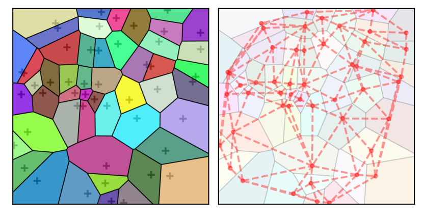
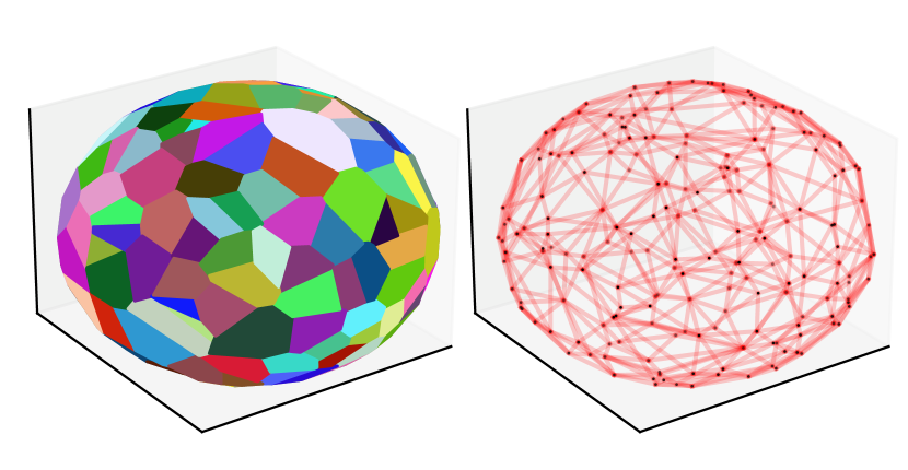
Figure 1: Voronoï cells and Delaunay triangulations on $[0,1]^{2}$ and $\mathbb{S}^{2}$.
(Made with Python package Matplotlib (Hunter, 2007))

Remark 6 (k-NN estimates).

A natural variant of the proposed method is obtained by replacing the $1$-NN estimate $\hat{\varphi}_{n}$ in Eq. (1) by a $k$-NN estimate $\hat{\varphi}_{n}^{(k)}$ which averages the evaluations of the $k$ nearest neighbors of a given point. The estimate is then defined by $\hat{\varphi}_{n}^{(k)}(x)=k^{-1}\sum_{j=1}^{k}\varphi(\hat{N}_{n,j}(x))$ where $\hat{N}_{n,j}(x)$ is the $j$-nearest neighbor of $x$. This involves both the tuning of the hyperparameter $k\geq 1$ and some extra computation due to the associated nearest neighbors search. In regression or classification, high values of $k$ can reduce the variance of the estimate by averaging the model noise at the cost of added computations. In contrast, the control neighbors estimate $(k=1)$ is free of these additional costs and takes advantage of the noiseless evaluations (Biau and Devroye, 2015, Chapter 15) of the integrand.

Remark 7 (Monte Carlo integration on manifolds).

The notion of nearest neighbors on $\mathbb{R}^{d}$ is defined through the Euclidean distance and can be easily extended to a manifold equipped with a metric. When integrating on a Riemannian manifold $\mathcal{M}$ (see for instance Barp et al., 2022), one can consider the control neighbors estimate with respect to the distance on $\mathcal{M}$ induced by the metric tensor. In this case, the parameter $d$ corresponds to the dimension of the manifold measured by $\mu$.

3 From nearest neighors to control neighbors

This section presents the mathematical framework of nearest neighbor estimates with reminders on Voronoi cells and central quantities for the analysis, namely the degree of a point and the average cell volume. Next, two control neighbor estimates are introduced and some basic properties are stated.

3.1 Nearest neighbors

Let $X_{1},\ldots,X_{n}$ be independent and identically distributed random vectors in $\mathbb{R}^{d}$, drawn from a distribution $\mu$ without atoms. Let $\|\cdot\|$ denote the Euclidean norm and let $x\in\mathbb{R}^{d}$ be a generic point.

Definition 1 (Nearest neighbors and distances).

The nearest neighbor $\hat{N}_{n}(x)$ of $x$ among $X_{1},\ldots,X_{n}$ and the associated distance $\hat{\tau}_{n}(x)$ are

$$\hat{N}_{n}(x)\in\operatornamewithlimits{\arg\min}_{Y\in\{X_{1},\dots,X_{n}\}}\|x-Y\|,\qquad\hat{\tau}_{n}(x)=\|\hat{N}_{n}(x)-x\|.$$

When the $\operatornamewithlimits{\arg\min}$ is not unique, $\hat{N}_{n}(x)$ is defined as the one point among the $\operatornamewithlimits{\arg\min}$ having the smallest index. More generally, for $k=1,\ldots,n$, let $\hat{N}_{n,k}(x)$ denote the $k$-nearest neighbor of $x$ and $\hat{\tau}_{n,k}(x)=\|\hat{N}_{n,k}(x)-x\|$ the associated distance, breaking ties by the lexicographic order.

The sample $\mathcal{X}_{n}=\{X_{1},\ldots,X_{n}\}$ defines a natural (random) partition of the integration domain when considering the associated Voronoi cells. Any such cell is associated to a given sample point, say $X_{i}$, and contains all the points $x$ of which the nearest neighbor is $X_{i}$.

Definition 2 (Voronoi cells and volumes).

The Voronoi cells of $X_{1},\ldots,X_{n}$ are

$$\forall i=1,\ldots,n,\qquad S_{n,i}=\left\{x\in\mathbb{R}^{d}:\,\hat{N}_{n}(x)=X_{i}\right\},$$

with Voronoi volumes $V_{n,i}=\mu(S_{n,i})$.

The $1$-NN estimate of $\varphi$ is defined as $\hat{\varphi}_{n}(x)=\varphi(\hat{N}_{n}(x))$ for all $x\in\mathbb{R}^{d}$ and is piece-wise constant on the Voronoi cells, i.e., $\hat{\varphi}_{n}(x)=\sum_{i=1}^{n}\varphi(X_{i})\operatorname{\mathds{1}}_{S_{n,i}}(x)$.

The leave-one-out rule is a general technique to introduce independence between the prediction and the evaluation points. It is used as a cross-validation strategy in order to tune hyper-parameters of statistical procedures (Stone, 1974; Craven and Wahba, 1978). The leave-one-out version of $\hat{\varphi}_{n}$ without the $i$-th particle is denoted by $\hat{\varphi}_{n}^{(i)}$ and is obtained in the exact same way as $\hat{\varphi}_{n}$ except that a slightly different sample—in which the $i$-th observation has been removed—is used.

Definition 3 (Leave-one-out neighbors, Voronoi cells and volumes).

Let $i\in\{1,\ldots,n\}$ and $\mathcal{X}_{n}^{(i)}=\{X_{1},\ldots,X_{n}\}\setminus\{X_{i}\}$. The leave-one-out neighbor of $x\in\mathbb{R}^{d}$ is

$$\hat{N}_{n}^{(i)}(x)\in\operatornamewithlimits{\arg\min}_{Y\in\mathcal{X}_{n}^{(i)}}\|x-Y\|.$$

When the above $\operatornamewithlimits{\arg\min}$ is not unique, $\hat{N}_{n}^{(i)}(x)$ is defined as the one point among the $\operatornamewithlimits{\arg\min}$ having the smallest index. The leave-one-out Voronoi cell $S_{n,j}^{(i)}$ denotes the $j$-th Voronoi cell in $\mathcal{X}_{n}^{(i)}$, i.e.,

$$\forall j\in\{1,\ldots,n\}\setminus\{i\},\qquad S_{n,j}^{(i)}=\left\{x\in\mathbb{R}^{d}:\,\hat{N}_{n}^{(i)}(x)=X_{j}\right\}.$$

The leave-one-out Voronoi volume is defined as $V_{n,j}^{(i)}=\mu(S_{n,j}^{(i)})$.

The leave-one-out $1$-NN predictor used in Section 2 to define the proposed integral estimate is $\hat{\varphi}_{n}^{(i)}(x)=\varphi(\hat{N}_{n}^{(i)}(x))$. A key property is that $\hat{\varphi}_{n}^{(i)}$ and $\hat{\varphi}_{n}$ coincide on $S_{n,j}$ for $j\neq i$. On the cell $S_{n,i}$, when the function $\varphi$ is Lipschitz, the supremum distance between $\hat{\varphi}_{n}^{(i)}$ and $\hat{\varphi}_{n}$ is of the same order as the nearest neighbor distance. In terms of the $L^{1}(\mu)$-norm, their difference is even smaller if the cell $S_{n,i}$ has a small $\mu$-volume. Relevant for our numerical integration problem is that the average of the integrals $\mu(\hat{\varphi}_{n}^{(i)})$ is close to $\mu(\hat{\varphi}_{n})$.

Lemma 1.

In terms of $\bar{\varphi}_{n}(x)=\sum_{i=1}^{n}\hat{\varphi}_{n}^{(i)}(x)\operatorname{\mathds{1}}_{S_{n,i}}(x)$, we have $\sum_{i=1}^{n}\{\mu(\hat{\varphi}_{n}^{(i)})-\mu(\hat{\varphi}_{n})\}=\mu(\bar{\varphi}_{n}-\hat{\varphi}_{n}).$

Enumerating how many times a point $X_{j}$ is the nearest neighbor of points $X_{i}$ for $i\neq j$ reflects how much $X_{j}$ is surrounded within the sample. Another important quantity that qualifies the isolation of a point $X_{j}$ is obtained by summing the Voronoi volumes $V_{n,j}^{(i)}$ over $i\neq j$. These two notions are formally stated in the next definition.

Definition 4 (Degree and cumulative volume).

For all $j=1,\ldots,n$, the degree $\hat{d}_{n,j}$ represents the number of times $X_{j}$ is a nearest neighbor of a point $X_{i}$ for $i\neq j$. The associated $j$-th cumulative Voronoi volume is denoted by $\hat{c}_{n,j}$, that is,

$$\hat{d}_{n,j}=\sum_{i:i\neq j}\operatorname{\mathds{1}}_{S_{n,j}^{(i)}}(X_{i})\qquad\text{and}\qquad\hat{c}_{n,j}=\sum_{i:i\neq j}V_{n,j}^{(i)}.$$

Interestingly, the degree of a point and its cumulative Voronoi volume have the same expectation: $\operatorname{\mathbb{E}}[\hat{d}_{n,j}]=\operatorname{\mathbb{E}}[\hat{c}_{n,j}]=1$. The two quantities $\hat{d}_{n,j}$ and $\hat{c}_{n,j}$ will be useful in the next section to express the control neighbors estimate as a linear integration rule. For now, we note that weighted sums of $\varphi(X_{j})$ using $\hat{d}_{n,j}$ and $\hat{c}_{n,j}$ as weights are related to the leave-one-out estimate.

Lemma 2.

It holds that

$$\sum_{i=1}^{n}\varphi(X_{i})\,\hat{d}_{n,i}=\sum_{i=1}^{n}\hat{\varphi}_{n}^{(i)}(X_{i})\qquad\text{ and }\qquad\sum_{i=1}^{n}\varphi(X_{i})\,\hat{c}_{n,i}=\sum_{i=1}^{n}\mu(\hat{\varphi}_{n}^{(i)}).$$

3.2 Control neighbors

With the help of previous notation, we now introduce the two control neighbor estimates

$$\hat{\mu}_{n}^{\mathrm{(NN)}}(\varphi) =\frac{1}{n}\sum_{i=1}^{n}\left[\varphi(X_{i})-\left\{\hat{\varphi}_{n}^{(i)}(X_{i})-\mu(\hat{\varphi}_{n})\right\}\right]$$ (1)

$$\hat{\mu}_{n}^{\mathrm{(NN-loo)}}(\varphi) =\frac{1}{n}\sum_{i=1}^{n}\left[\varphi(X_{i})-\left\{\hat{\varphi}_{n}^{(i)}(X_{i})-\mu(\hat{\varphi}_{n}^{(i)})\right\}\right].$$ (2)

The first one, $\hat{\mu}_{n}^{\mathrm{(NN)}}(\varphi)$, is the output in the nearest neighbor algorithm in Section 2. The second one, $\hat{\mu}_{n}^{\mathrm{(NN-loo)}}(\varphi)$, is a slight modification of $\hat{\mu}_{n}^{\mathrm{(NN)}}(\varphi)$ that is an unbiased estimate of $\mu(\varphi)$. A simple conditioning argument implies that

$$\operatorname{\mathbb{E}}\left[\hat{\varphi}_{n}^{(i)}(X_{i})-\mu(\hat{\varphi}_{n}^{(i)})\right]=\operatorname{\mathbb{E}}\left[\operatorname{\mathbb{E}}\left[\hat{\varphi}_{n}^{(i)}(X_{i})-\mu(\hat{\varphi}_{n}^{(i)})\,\Big{|}\,\mathcal{X}_{n}^{(i)}\right]\right]=0,$$

which is sufficient to get the zero-bias property

$$\operatorname{\mathbb{E}}\left[\hat{\mu}_{n}^{\mathrm{(NN-loo)}}(\varphi)\right]=\mu(\varphi).$$

Moreover, since $\hat{\varphi}_{n}^{(i)}$ is similar to the $1$-NN estimate $\hat{\varphi}_{n}$ of $\varphi$ based on the full sample $X_{1},\ldots,X_{n}$, their integrals should be close. This intuition is confirmed in Proposition 2 in Appendix A in the supplementary material. Consequently, the estimate (2) will play an important role in the theory. However, computing the terms $\mu(\hat{\varphi}_{n}^{(i)})$ for $i=1,\ldots,n$ requires the evaluation of $n$ additional integrals. In practice, the working estimate is (1) as it involves less computations. Further, it is worthwhile to note that our two control neighbor estimates are not based on a single approximation of the integrand $\varphi$ but rather on $n$ different approximations $\hat{\varphi}_{n}^{(i)}$.

The two control neighbor estimates in (1) and (2) can be expressed as linear integration rules of the form $\sum_{i=1}^{n}w_{i,n}\,\varphi(X_{i})$ with weights $w_{i,n}$ not depending on the integrand $\varphi$. The weights involve the degrees $\hat{d}_{n,i}$ and the (cumulative) volumes ${V}_{n,i}$ and $\hat{c}_{n,i}$ in Definitions 2 and 4.

Proposition 1 (Quadrature rules).

The estimates $\hat{\mu}_{n}^{\mathrm{(NN)}}(\varphi)$ and $\hat{\mu}_{n}^{\mathrm{(NN-loo)}}(\varphi)$ can be expressed as linear estimates of the form

$$\hat{\mu}_{n}^{\mathrm{(NN-loo)}}(\varphi)=\sum_{i=1}^{n}w_{i,n}^{\mathrm{(NN-loo)}}\varphi(X_{i})\quad\text{ and }\quad\hat{\mu}_{n}^{\mathrm{(NN)}}(\varphi)=\sum_{i=1}^{n}w_{i,n}^{\mathrm{(NN)}}\varphi(X_{i})$$

where $w_{i,n}^{\mathrm{(NN-loo)}}=(1+\hat{c}_{n,i}-\hat{d}_{n,i})/n$ and $w_{i,n}^{\mathrm{(NN)}}=(1+nV_{n,i}-\hat{d}_{n,i})/n$.

The weights of the two estimates satisfy $\sum_{i=1}^{n}w_{i,n}=1$, meaning that the integration rules are exact for constant functions. In the light of Proposition 1, the proposed estimate $\hat{\mu}_{n}^{\mathrm{(NN)}}(\varphi)$ consists in a simple modification of $\hat{\mu}_{n}^{\mathrm{(NN-loo)}}(\varphi)$ by replacing $\hat{c}_{n,i}$, which involves $n-1$ Voronoi volumes, by $nV_{n,i}$. The difference between both is of the order $n^{-1/2-1/d}$ as shown in the next section.

4 Main results

This section gathers some technical result on nearest neighbors before stating the main theoretical properties of the control neighbor estimates (1) and (2). Under suitable conditions on $\mu$ and $\varphi$, their mean squared errors are shown to reach the optimal rate as $\operatorname{\mathbb{E}}[|\hat{\mu}_{n}(\varphi)-\mu(\varphi)|^{2}]^{1/2}\lesssim n^{-1/2}n^{-1/d}$, where two positive sequences $a_{n}$ and $b_{n}$ satisfy $a_{n}\lesssim b_{n}$ provided $a_{n}\leq Cb_{n}$ for some constant $C>0$. Further, their finite-sample performance is studied through a concentration inequality providing a high-probability bound on the error $|\hat{\mu}_{n}(\varphi)-\mu(\varphi)|$.

4.1 Technical results on nearest neighbors

For the analysis, we consider the following assumptions which are related to the strong density assumption of Audibert and Tsybakov (2007). This condition ensures that the density $f$ of the measure $\mu$ has a sufficiently regular support and that it is bounded away from zero and infinity. Let $B(x,r)$ denote the ball with centre $x\in\mathbb{R}^{d}$ and radius $r>0$.

1. $X,X_{1},X_{2},\ldots$ are independent and identically distributed random vectors in $\mathbb{R}^{d}$ with common distribution $\mu$ having support $\mathcal{X}\subset\mathbb{R}^{d}$.

2. The measure $\mu$ admits a density $f$ with respect to the $d$-dimensional Lebesgue measure $\lambda_{d}$. There exist constants $b,U,c,r_{0}\in(0,\infty)$ with $b\leq U$ such that

   • $\forall x\in\mathcal{X},\quad b\leq f(x)\leq U$,

   • $\forall 0<r\leq r_{0},\forall x\in\mathcal{X},\quad\lambda_{d}(\mathcal{X}\cap B(x,r))\geq c\lambda_{d}(B(x,r))$.

3. The function $\varphi:\mathbb{R}^{d}\to\mathbb{R}$ is Lipschitz, i.e., there exists $L>0$ such that

   $$\forall x,y\in\mathbb{R}^{d},\quad|\varphi(x)-\varphi(y)|\leq L\left\|{x-y}\right\|.$$

Condition (A2) implies that the support $\mathcal{X}$ is bounded, since it is contained in a finite number of balls of radius $r_{0}$. Under (A3), we have $|\hat{\varphi}_{n}(x)-\varphi(x)|\leq L\hat{\tau}_{n}(x)$ for all $x\in\mathbb{R}^{d}$, so that the distance $\hat{\tau}_{n}$ is key in the analysis of the functional approximation problem of $\varphi$ by the estimate $\hat{\varphi}_{n}$. The next lemma provides control on the distance $\hat{\tau}_{n}(x)$ and follows from standard considerations in the $k$-NN literature (Biau and Devroye, 2015). Let $\Gamma$ denote the Euler gamma function and $V_{d}=\lambda_{d}(B(0,1))$ the volume of the unit ball in $\mathbb{R}^{d}$.

Lemma 3 (Bounding moments of nearest neighbor distances).

Under (A1) and (A2), we have, for any $q\geq 1$,

$$\forall x\in\mathcal{X},\quad\operatorname{\mathbb{E}}[\hat{\tau}_{n}(x)^{q}]\leq\left(nV_{d}bc\right)^{-q/d}\Gamma(q/d+1).$$

Furthermore, if $2k\leq n$, we have

$$\forall x\in\mathcal{X},\quad\operatorname{\mathbb{E}}[\hat{\tau}_{n,k}(x)^{q}]\leq 2^{2q/d+1}\Gamma(q/d+1)(nV_{d}bc/k)^{-q/d}.$$

Because of the proof technique, the case $k=1$ in the second inequality in Lemma 3 gives a looser bound than the first inequality.

Remark 8.

(Lower bounds) The uniform lower bounds in Condition (A2) play an important role in the analysis of nearest neighbor estimates as they allow a uniform control on the Voronoi cell diameters. Such a uniform bound is key to study the convergence of general $k$-NN estimates. For densities with general supports, one can also guarantee that no region is empty by some minimal mass assumption (Gadat et al., 2016). The question of necessary conditions for general uniform bounds remains an active field of research with recent progress for distributions with unbounded support (Kohler et al., 2006) and relaxations through tail assumptions (Gadat et al., 2016). Extending the present analysis to such general measures is left for further research.

4.2 Mean-squared error bounds

The main result of this section provides a finite-sample bound on the mean-squared error of the two control neighbors estimates in (1) and (2). The leave-one-out version $\hat{\mu}_{n}^{\mathrm{(NN-loo)}}$ involves $n$ additional integrals and is computationally cumbersome. The proposed estimate $\hat{\mu}_{n}^{\mathrm{(NN)}}$ requires only a single additional integral while remaining close to the leave-one-out estimate, since

$$\hat{\mu}_{n}^{\mathrm{(NN)}}(\varphi)-\hat{\mu}_{n}^{\mathrm{(NN-loo)}}(\varphi)=\mu(\hat{\varphi}_{n})-\frac{1}{n}\sum_{i=1}^{n}\mu(\hat{\varphi}_{n}^{(i)}).$$

Using this property and Lemma 1, we obtain that the mean-squared distance between the leave-one-out version and the proposed estimate is of order $\mathcal{O}(n^{-1/2-1/d})$ as $n\to\infty$; see Proposition 2 in Appendix A of the supplementary material for a precise statement. Therefore, the two estimates share the same convergence rate.

Theorem 1 (Mean squared error bounds).

Under (A1), (A2) and (A3), if $n\geq 4$, then

$$\operatorname{\mathbb{E}}\left[\bigl{|}\hat{\mu}_{n}^{\mathrm{(NN-loo)}}(\varphi)-\mu(\varphi)\bigr{|}^{2}\right]^{1/2} \leq C_{\mathrm{NN-loo}}n^{-1/2}n^{-1/d},$$

$$\operatorname{\mathbb{E}}\left[\bigl{|}\hat{\mu}_{n}^{\mathrm{(NN)}}(\varphi)-\mu(\varphi)\bigr{|}^{2}\right]^{1/2} \leq C_{\mathrm{NN}}n^{-1/2}n^{-1/d},$$

where

$$C_{\mathrm{NN-loo}} =16L\left(V_{d}bc\right)^{-1/d}(U/bc)^{-1/2},$$

$$C_{\mathrm{NN}} =39L(V_{d}bc)^{-1/d}(U/bc)^{-1/2}.$$

The rates obtained in Theorem 1 match the complexity rate stated in Novak (2016), see Section 1. The results in the aforementioned paper are concerned about a slightly more precise context as they assert that no random integration rule (see the paper for more details) can reach a higher accuracy—measured in terms of mean-squared error—than $\mathcal{O}(n^{-1-2/d})$ when the integration measure is the uniform distribution on the unit cube and the integrand is Lipschitz. Theorem 1 states that the optimal rate is in fact achieved by some integration rule in situations where the integration measure’s density is not necessarily uniform but merely bounded from below and above.

The control neighbors estimates involve an approximation of $\varphi$ by piece-wise constant functions $\hat{\varphi}_{n}^{(i)}$ and therefore cannot achieve an acceleration of the convergence rate of more than $n^{-1/d}$. It is an interesting question whether a higher-order nearest neighbor approximation can achieve a greater accuracy for integrands that are smoother than just Lipschitz. The simulation experiments in Section 5 will give some feeling on the actual improvement of the control neighbors estimate over the basic Monte Carlo method at finite sample sizes.

4.3 Concentration inequalities

In order to obtain a finite-sample performance guarantee of the proposed estimates, we apply an extension of McDiarmid’s concentration inequality for functions with bounded differences on a high probability set $A$. The inequality is stated in Theorem 3 in Appendix A of the supplementary material and is itself a minor extension of an inequality due to Combes (2015).

In combination with (A2), Assumption (A3) implies that $\varphi$ is uniformly bounded on $\mathcal{X}$, since $\mathcal{X}$ has a finite diameter. Write $C_{\varphi}=\frac{1}{2}\left\{\sup_{x\in\mathcal{X}}\varphi(x)-\inf_{x\in\mathcal{X}}\varphi(x)\right\}$. The two control neighbor estimates satisfy the following concentration inequalities.

Theorem 2 (Concentration inequalities).

Under (A1), (A2) and (A3), we have, for any $\varepsilon\in(0,1)$, with probability at least $1-\varepsilon$,

$$\left|{\hat{\mu}_{n}^{\mathrm{(NN-loo)}}(\varphi)-\mu(\varphi)}\right| \leq C_{1}\Delta_{n,\varepsilon}+\frac{6C_{\varphi}}{n^{1/2+1/d}}\qquad\text{and}$$

$$\left|{\hat{\mu}_{n}^{\mathrm{(NN)}}(\varphi)-\mu(\varphi)}\right| \leq C_{2}\Delta_{n,\varepsilon}+\frac{6C_{\varphi}}{n^{1/2+1/d}}+\frac{(2^{3/d+1}+1)L(V_{d}bc)^{-1/d}}{n^{1+1/d}},$$

where

$$\Delta_{n,\varepsilon}=\frac{\sqrt{\log(2/\sqrt{\varepsilon})}+\frac{1}{n^{1/d}}}{n^{1/2+1/d}}\cdot\begin{dcases}\log(24n/\varepsilon)^{1+1/d}&\text{ for }\varepsilon\leq\frac{2}{n^{1/2+1/d}},\\ (3\log(3n))^{1+1/d}&\text{ for }\varepsilon>\frac{2}{n^{1/2+1/d}}.\end{dcases}$$

The values of $C_{1},C_{2}>0$ depend on $(b,c,d,L,U)$ and are provided explicitly in the proof.

For small but fixed $\varepsilon\in(0,1)$, the concentration inequalities state that the probability that the error $\left|{\hat{\mu}_{n}(\varphi)-\mu(\varphi)}\right|$ is larger than a constant multiple of $\sqrt{\log(1/\varepsilon)}(\log n)^{1+1/d}n^{-1/2}n^{-1/d}$ is less than $\varepsilon$. The additional logarithmic factor in Theorem 2 in comparison to Theorem 1 comes from the need to exert uniform control on the largest nearest neighbor distance via Lemma 5 in Appendix A in the supplement, which in turn originates from Portier (2023).

5 Numerical experiments

This section gather several experiments that highlight the wide range of applications of the proposed control neighbors estimate. To illustrate its finite-sample performance, we first present in Section 5.1 some examples involving integration problems on different spaces: first on the unit cube $[0,1]^{d}$ and on $\mathbb{R}^{d}$ with uniform and Gaussian measures respectively; then a more complex integration problem dealing with the moments of random orthogonal matrices; finally a challenging problem dealing with the integration of some smooth functions on the sphere $\mathbb{S}^{2}$. Then, Section 5.2 deals with the application of Monte Carlo estimates for optimal transport when computing the Sliced-Wasserstein distance. Additional experiments on a finance application with Monte Carlo exotic option pricing are available in Appendix E of the supplement.

In all experiments, MC represents the naive Monte Carlo estimate and CVNN returns the value of $\hat{\mu}_{n}^{\mathrm{(NN)}}(\varphi)$ for which the integral $\mu(\varphi_{n})$ is replaced by a Monte Carlo estimate that uses $M=n^{2}$ particles, with $n$ the number of evaluations of $\varphi$.

5.1 Integration on various spaces: $[0,1]^{d},\mathbb{R}^{d},O_{m}(\mathbb{R})$ and $\mathbb{S}^{q-1}$

The aim of this section is to empirically validate the $\mathcal{O}(n^{-1/2}n^{-1/d})$ convergence rate of the control neighbors estimate in a wide variety of integration problems ranging from standard Euclidean spaces such as the unit cube $[0,1]^{d}$ or the group of orthogonal matrices $O_{m}(\mathbb{R})$ to non-Euclidean spaces such as the sphere $\mathbb{S}^{q-1}$. In the different settings, the sample size evolves from $n=10^{1}$ to $n=10^{4}$ and the figures report the evolution of the root mean squared error $n\mapsto\operatorname{\mathbb{E}}[|\hat{\mu}_{n}^{\mathrm{(NN)}}(\varphi)-\mu(\varphi)|^{2}]^{1/2}$ where the expectation is computed over $100$ independent replications.

Integration on $[0,1]^{d}$ and $\mathbb{R}^{d}$. Consider first the integration problem $\mu(\varphi)=\int\varphi\,\mathrm{d}\mu$ where the measure $\mu$ is either the uniform distribution over the unit cube $[0,1]^{d}$ or the multivariate Gaussian measure on $\mathbb{R}^{d}$. The goal is to compute $\int\varphi_{1}(x)\operatorname{\mathds{1}}_{[0,1]^{d}}(x)\,\mathrm{d}x$ and $\int\varphi_{2}(x)\psi(x)\,\mathrm{d}x$ with

$$\textstyle\varphi_{1}(x_{1},\ldots,x_{d})=\sin\left(\pi\left(\frac{2}{d}\sum_{i=1}^{d}x_{i}-1\right)\right)\quad\text{ and }\quad\varphi_{2}(x_{1},\ldots,x_{d})=\sin\left(\frac{\pi}{d}\sum_{i=1}^{d}x_{i}\right)$$ (3)

and with $\psi(\cdot)$ the probability density function of the multivariate Gaussian distribution $\mathcal{N}(0,I_{d})$. Figure 2 displays the evolution of the root mean squared error for the two integrals in dimension $d\in\{2,3,4\}$. The different error curves confirm the optimal convergence rate $\mathcal{O}(n^{-1/2}n^{-1/d})$ for the control neighbors estimate. In dimension $d=2$ and $d=3$, the root mean squared error of the CVNN estimate can be reduced by a factor ten compared to the standard Monte Carlo approach.

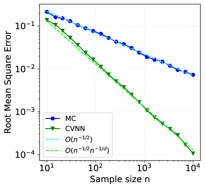
(a) $\varphi_{1},d=2$

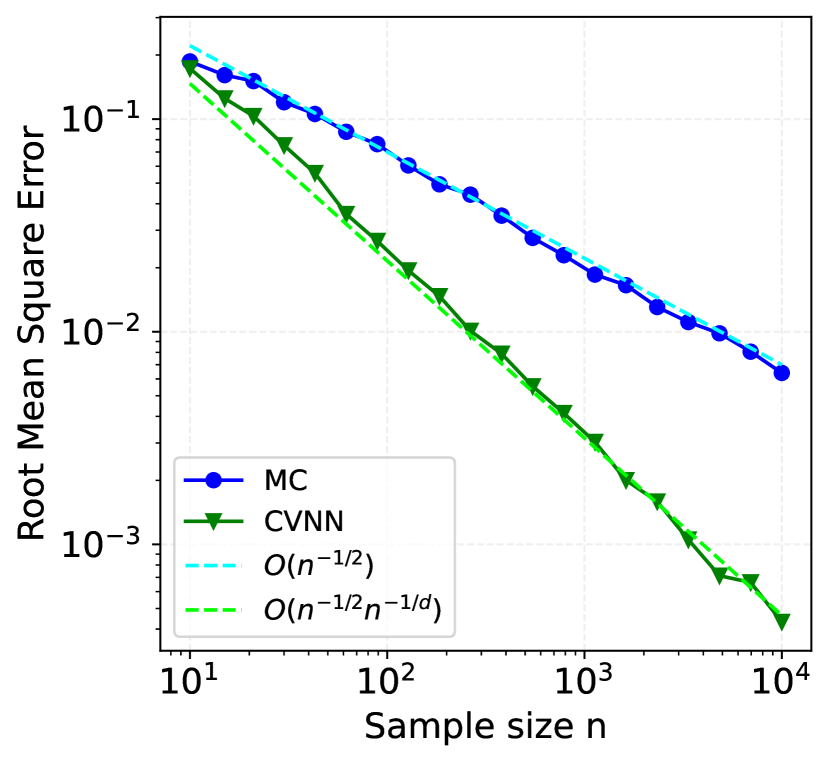
(b) $\varphi_{1},d=3$

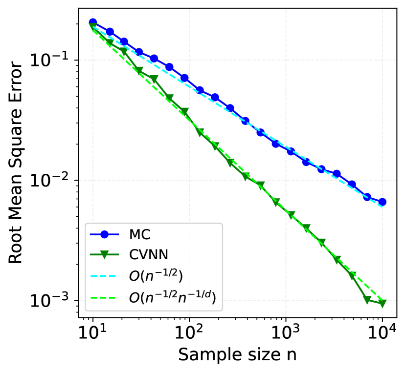
(c) $\varphi_{1},d=4$

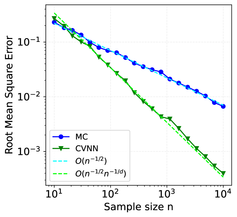
(d) $\varphi_{2},d=2$

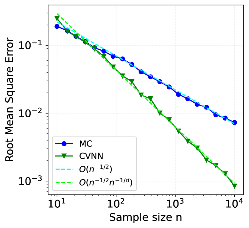
(e) $\varphi_{2},d=3$

(f) $\varphi_{2},d=4$

Figure 2: Root mean squared errors obtained over $100$ replications for functions $\varphi_{1}$ (top) and $\varphi_{2}$ (bottom) in Eq. (3) in dimension $d\in\{2,3,4\}$ (left to right).

Integration on the orthogonal group $O_{m}(\mathbb{R)}$. Consider the group of real orthogonal matrices $O_{m}(\mathbb{R})=\{X\in\mathrm{GL}_{m}(\mathbb{R}):X^{\top}X=XX^{\top}=\mathrm{I}_{m}\}$ and the moments of the trace of a random orthogonal matrix, i.e., integrands of the form $\varphi_{k}:O_{m}(\mathbb{R})\to\mathbb{R}$ with $\varphi_{k}(X)=\operatorname{tr}(X)^{k}$. The goal is to compute the integrals

$$a_{k}=\mu(\varphi_{k})=\int_{O_{m}(\mathbb{R})}\operatorname{tr}(X)^{k}\,\mathrm{d}\mu(X),$$ (4)

with $\mathrm{d}\mu(X)$ the Haar measure on $O_{m}(\mathbb{R})$. Note that this measure is well defined since $O_{m}(\mathbb{R})$ is a compact set and in view of Remark 7, the underlying dimension of interest is $d=m(m-1)/2$. In practice, random orthogonal matrices $X_{1},\ldots,X_{n}\in O_{m}(\mathbb{R})$ are generated using the function ortho_group of the Python package scipy (Virtanen et al., 2020). This function returns random orthogonal matrices drawn from the Haar distribution using a careful QR decomposition as in Mezzadri (2007). The nearest neighbors are computed using the norm associated to the Frobenius inner product $\langle X,Y\rangle=\operatorname{tr}(X^{\top}Y)$ for $X,Y\in O_{m}(\mathbb{R})$. Figure 3 reports the evolution of the root mean squared error and boxplots of the normalized error $(\hat{\mu}_{n}^{\mathrm{(NN)}}(\varphi)-\mu(\varphi))/\mu(\varphi)$ for integrands $\varphi_{1}$ and $\varphi_{2}$ over the group $O_{3}(\mathbb{R})$ which corresponds to dimension $d=3$. Once again, the experiments empirically validate the convergence rates of the Monte Carlo methods and reveal the variance reduction obtained with the control neighbors estimate.

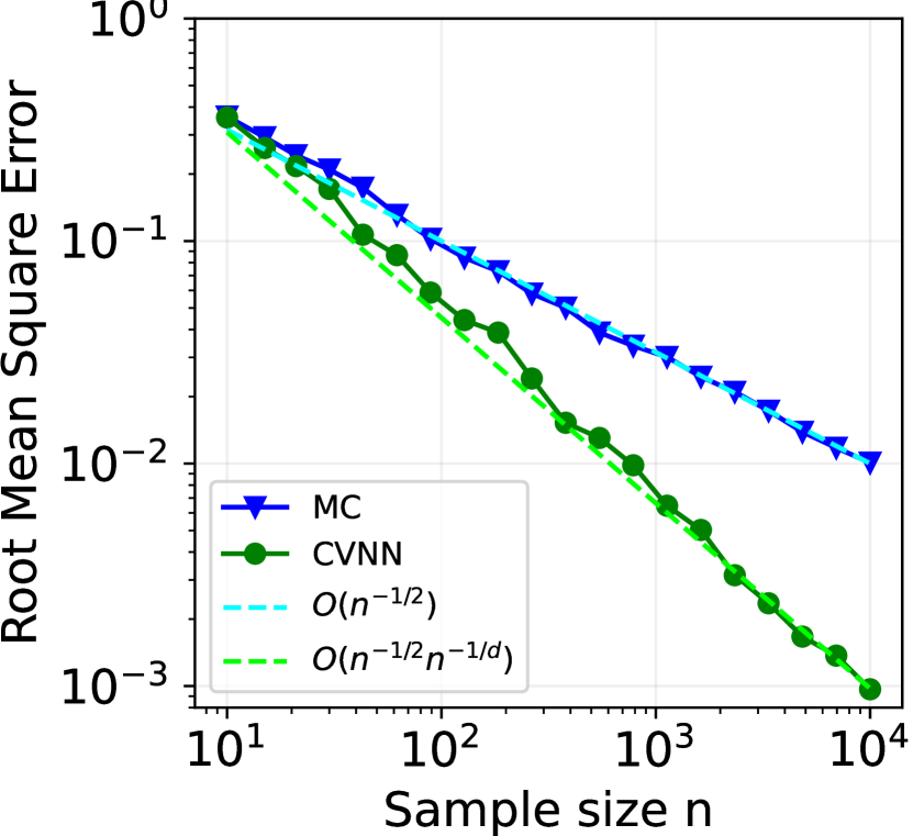
(a) RSME for $a_{1}$

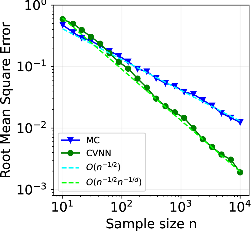
(b) RMSE for $a_{2}$

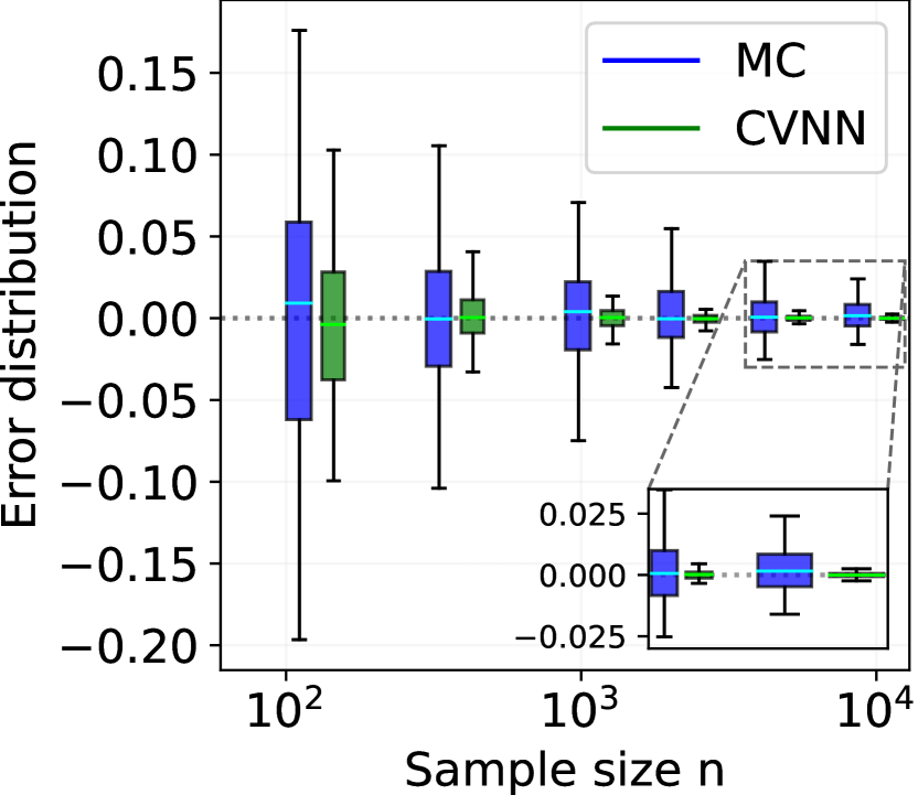
(c) Boxplot for $a_{1}$

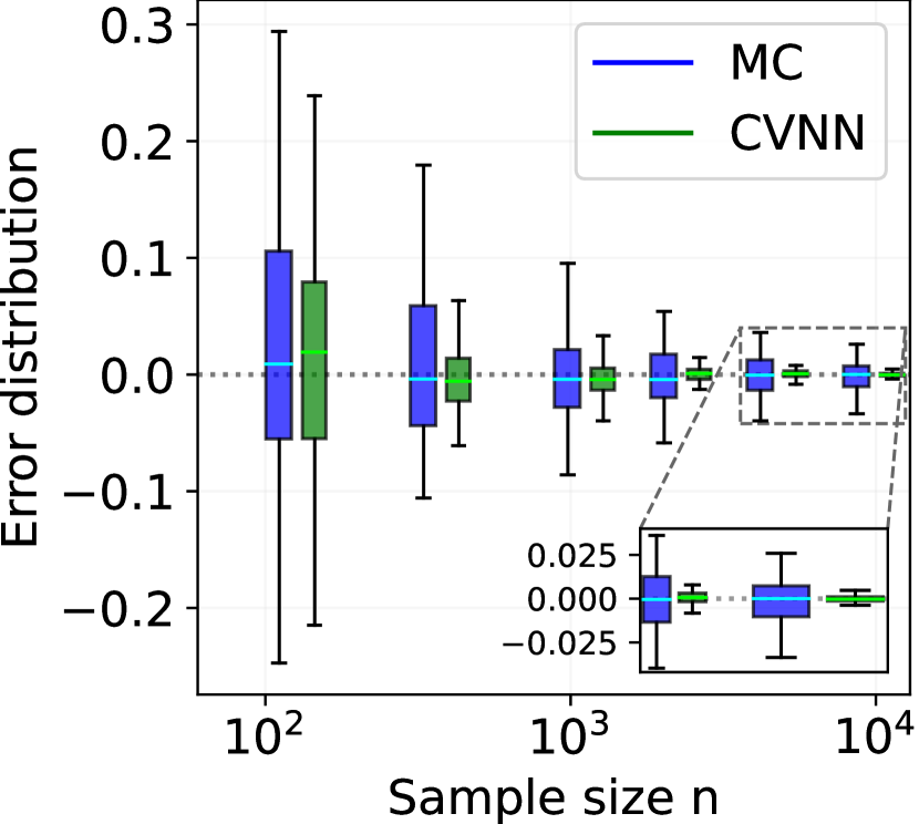
(d) Boxplot for $a_{2}$

Figure 3: Root mean squared errors (left) and boxplots of the errors (right) obtained over $100$ replications for functions $\varphi_{1}$ and $\varphi_{2}$ in Eq. (4) over the group $O_{3}(\mathbb{R})$.

Integration on the sphere $\mathbb{S}^{2}$. Consider the sphere $\mathbb{S}^{2}$ embedded in $\mathbb{R}^{3}$. This is a non-Euclidean manifold of dimension $d=2$ with positive curvature and the distances on the sphere are computed using the equations of the great circles. Consider the integral $\int_{\mathbb{S}^{2}}\varphi\,\mathrm{d}\Omega$ with $\Omega$ the uniform distribution on $\mathbb{S}^{2}$ and integrands

$$\varphi_{3}(x,y,z)=\cos(x+y+z),\quad\varphi_{4}(x,y,z)=\cos(x)\cos(y)\cos(z),\quad\varphi_{5}(x,y,z)=\exp(x-y)$$ (5)

so that $\mu(\varphi_{3})=\mu(\varphi_{4})=(4\pi/\sqrt{3})\sin(\sqrt{3})$ and $\mu(\varphi_{5})=\pi\sqrt{8}\sinh(\sqrt{2})$. Figure 4 below reports the evolution of the root mean squared error and the boxplots of the errors over the sphere $\mathbb{S}^{2}$. The error curves empirically validate the $\mathcal{O}(n^{-1})$ convergence rate for the control neighbors estimate while the boxplots highlight the variance reduction of the proposed method.

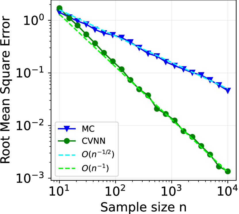
(a) RMSE $\varphi_{3}$

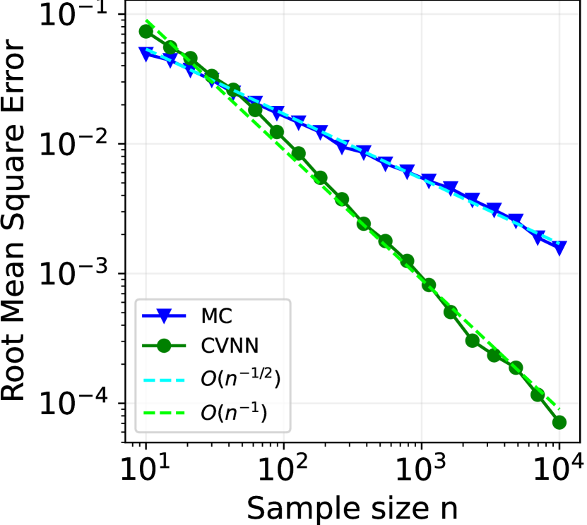
(b) RMSE $\varphi_{4}$

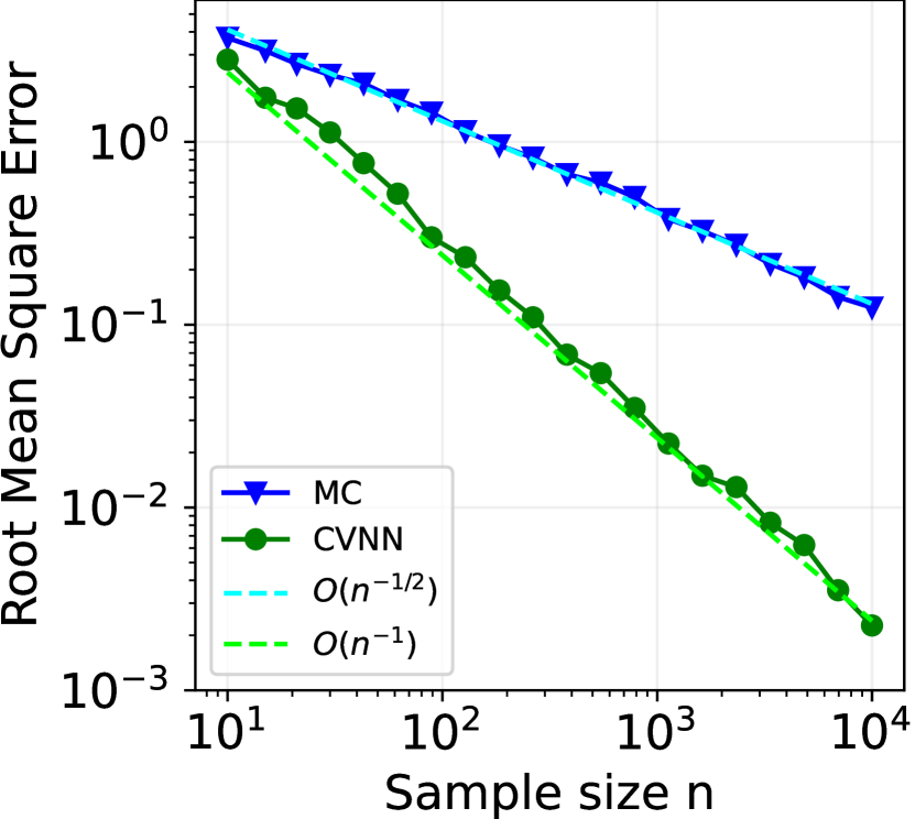
(c) RMSE $\varphi_{5}$

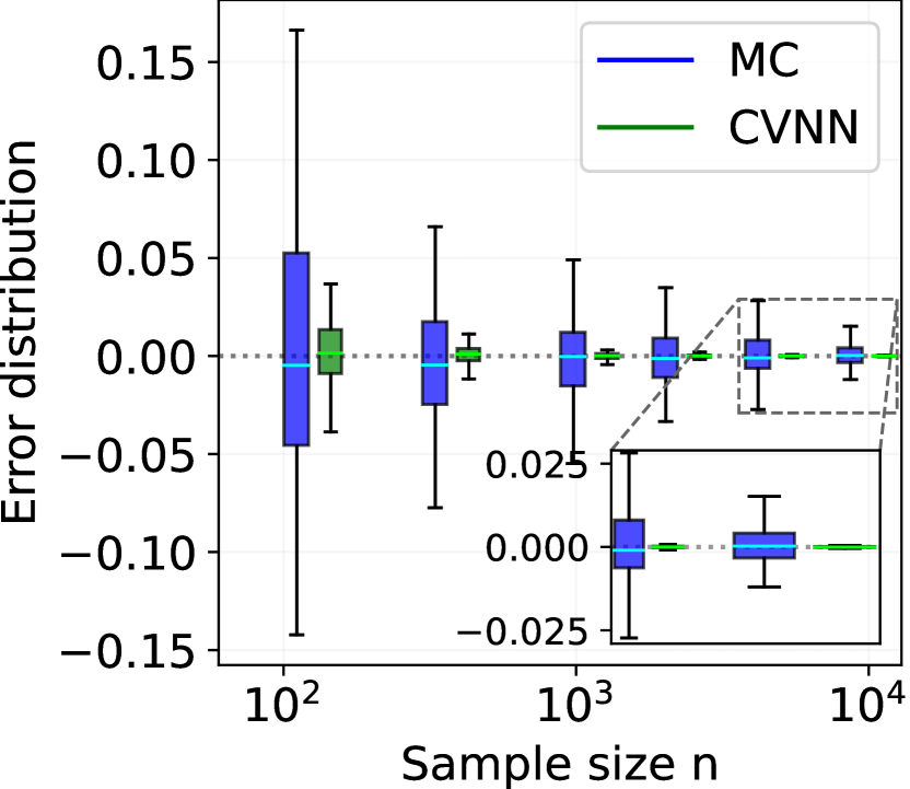
(d) Boxplot $\varphi_{3}$

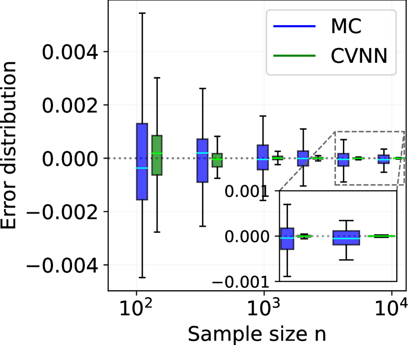
(e) Boxplot $\varphi_{4}$

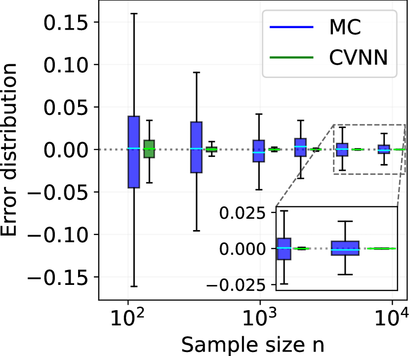
(f) Boxplot $\varphi_{5}$

Figure 4: Root mean squared errors (top) and boxplots of the errors (bottom) obtained over $100$ replications for functions $\varphi_{3}$ (left), $\varphi_{4}$ (middle) and $\varphi_{5}$ (right) in Eq. (5) when integrating over $\mathbb{S}^{2}$.

5.2 Monte Carlo Integration for Optimal Transport

Optimal transport. Optimal transport (OT) is a mathematical framework for measuring the distance between probability distributions. It has proven to be particularly useful in machine learning applications, where it can be used for tasks such domain adaptation (Courty et al., 2017) and image generation (Gulrajani et al., 2017; Genevay et al., 2018). The recent development of efficient algorithms for solving optimal transport problems, e.g., the Sliced-Wasserstein (SW) distance (Rabin et al., 2012) and Sinkhorn distance (Cuturi, 2013), has made it a practical tool for large-scale machine learning applications.

OT distances. For $\mathsf{X}\subseteq\mathbb{R}^{q}$, denote by $\mathcal{P}(\mathsf{X})$ the set of probability measures supported on $\mathsf{X}$ and let $p\in[1,\infty)$. The Wasserstein distance of order $p$ between $\mu,\nu\in\mathcal{P}(\mathsf{X})$ is

$$W_{p}^{p}(\mu,\nu)=\inf_{\pi\in\Pi(\mu,\nu)}\int_{\mathsf{X}\times\mathsf{X}}\|x-y\|^{p}\,\mathrm{d}\pi(x,y),$$

where $\Pi(\mu,\nu)\subset\mathcal{P}(\mathsf{X}\times\mathsf{X})$ denotes the set of couplings for $(\mu,\nu)$, i.e., probability measures whose marginals with respect to the first and second variables are $\mu$ and $\nu$ respectively. While the Wasserstein distance enjoys attractive theoretical properties (Villani, 2009, Chapter 6), it suffers from a high computational cost. When computing $W_{p}(\mu_{m},\nu_{m})$ for discrete distributions $\mu_{m}$ and $\nu_{m}$ supported on $m$ points, the worst-case computational complexity scales as $\mathcal{O}(m^{3}\log m)$ (Peyré et al., 2019). To overcome this issue, the Sliced-Wasserstein distance takes advantage of the fast computation of the Wasserstein distance between univariate distributions $\mu,\nu\in\mathcal{P}(\mathbb{R})$. Indeed, for $\mu_{m}=(1/m)\sum_{i=1}^{m}\delta_{x_{i}}$ and $\nu_{m}=(1/m)\sum_{i=1}^{m}\delta_{y_{i}}$ with $x_{i},y_{i}\in\mathbb{R}$, the $W_{p}$-distance involves sorting the atoms $x_{(1)}\leq\ldots\leq x_{(m)}$ and $y_{(1)}\leq\ldots\leq y_{(m)}$, yielding

$$W_{p}^{p}(\mu_{m},\nu_{m})=\frac{1}{m}\sum_{i=1}^{m}|x_{(i)}-y_{(i)}|^{p},$$

leading to a complexity of $\mathcal{O}(m\log m)$ operations induced by the sorting step.

Recall that $\mathbb{S}^{q-1}=\{\theta\in\mathbb{R}^{q}:\|\theta\|=1\}$ is the unit sphere of $\mathbb{R}^{q}$ and let $\theta^{\star}:\mathbb{R}^{q}\to\mathbb{R}$ denote the linear map $\theta^{\star}(x)=\langle\theta,x\rangle$ for $x\in\mathbb{R}^{d}$. Let $\rho\in\mathcal{P}(\mathbb{S}^{q-1})$. The Sliced-Wasserstein (SW) distance (Rabin et al., 2012; Bonneel et al., 2015; Kolouri et al., 2019) of order $p$ based on $\rho$ is defined for $\mu,\nu\in\mathcal{P}(\mathsf{X})$ as

$$SW_{p}^{p}(\mu,\nu,\rho)=\operatorname{\mathbb{E}}_{\theta}[W_{p}^{p}(\theta_{\#}^{\star}\mu,\theta_{\#}^{\star}\nu)]=\int_{\mathbb{S}^{d-1}}W_{p}^{p}(\theta_{\#}^{\star}\mu,\theta_{\#}^{\star}\nu)\,\mathrm{d}\rho(\theta),$$ (6)

where $f_{\#}\xi$ is the push-forward measure of $\xi\in\mathcal{P}(\mathbb{R}^{q})$ by a measurable function $f$ on $\mathbb{R}^{d}$. For $\theta\in\mathbb{S}^{q-1}$, the measures $\theta_{\#}^{\star}\mu$ and $\theta_{\#}^{\star}\nu$ are the distributions of the projections $\langle\theta,X\rangle$ and $\langle\theta,Y\rangle$ of random vectors $X$ and $Y$ on $\mathbb{R}^{q}$ with distributions $\mu$ and $\nu$, respectively. In practice, the random directions $\theta_{1},\ldots,\theta_{n}$ are sampled independently from the uniform distribution on the unit sphere $\mathbb{S}^{q-1}$ and the SW-distance of Eq. (6) is approximated using a standard Monte Carlo estimate with $n$ random projections as

$$\widehat{SW}_{p}^{p}(\mu_{m},\nu_{m})=\frac{1}{n}\sum_{i=1}^{n}W_{p}^{p}((\theta_{i})_{\#}^{\star}\mu_{m},(\theta_{i})_{\#}^{\star}\nu_{m}).$$

Multivariate Gaussians. The goal is to compare the variance of the standard Monte Carlo estimate (SW-MC) with the proposed control neighbors estimate (SW-CVNN) when computing the Sliced-Wasserstein distance between Gaussian distributions. More precisely we want to compute $SW_{2}(\mu,\nu)=SW_{2}(\mu,\nu,\rho)$ with respect to the uniform distribution $\rho$ on the unit sphere, where $\mu=\mathcal{N}_{q}(m_{X},\sigma_{X}^{2}\mathrm{I}_{q})$ and $\nu=\mathcal{N}_{q}(m_{Y},\sigma_{Y}^{2}\mathrm{I}_{q})$ with $m_{X},m_{Y}\sim\mathcal{N}(0,\mathrm{I}_{q})$ and $\sigma_{X}=2$ and $\sigma_{Y}=5$. We consider the corresponding empirical distributions $\mu_{m}$ and $\nu_{m}$ based on $m=2\,000$ samples and compute the Monte Carlo estimates of the SW₂ distance using a number of projections $n\in\{50;100;250;500;1000\}$ in dimension $q\in\{3;6\}$. In the notation of the general theory, we have $d=(q-1)\in\{2;5\}$ since we are integrating over the $(q-1)$-dimensional sphere in $\mathbb{R}^{q}$. Figure 5 below shows the error distribution of the different Monte Carlo estimates (SW-MC and SW-CVNN) of the SW₂ distance where the exact value (see (Nadjahi et al., 2021, Appendix S3.1)) is given by

$$SW_{2}^{2}(\mathcal{N}_{q}(m_{X},\sigma_{X}^{2}\mathrm{I}_{q}),\mathcal{N}_{q}(m_{Y},\sigma_{Y}^{2}\mathrm{I}_{q}))=\frac{1}{q}\|m_{X}-m_{Y}\|_{2}^{2}+(\sigma_{X}-\sigma_{Y})^{2}.$$

The different boxplots highlight the good performance of the proposed control neighbors estimate in terms of variance reduction.

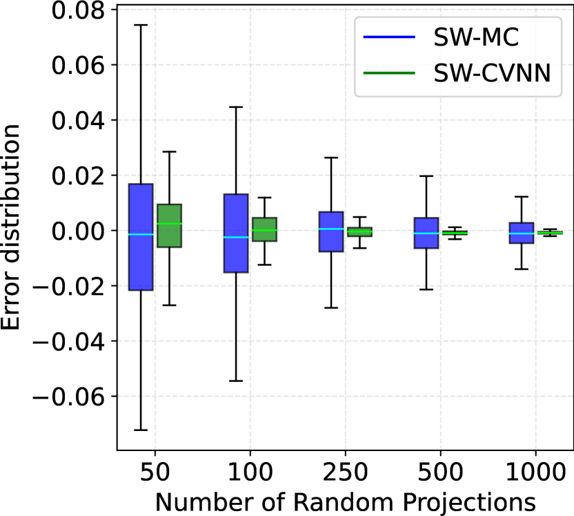
(a) $SW_{2},\ q=3$

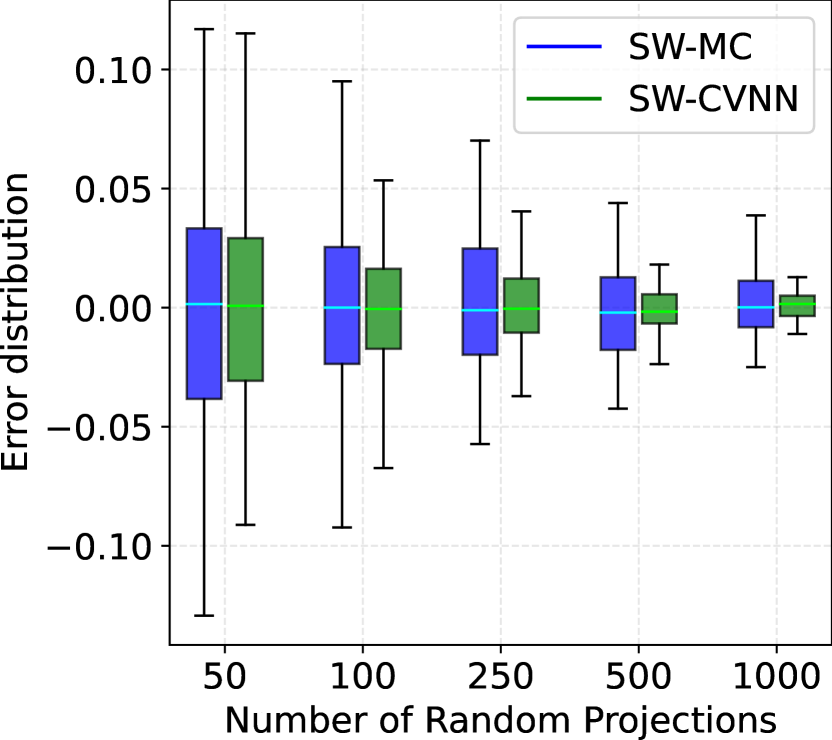
(b) $SW_{2},\ q=6$

Figure 5: Boxplots of Sliced-Wasserstein estimates SW-MC and SW-CVNN for Gaussian distributions on $\mathbb{R}^{q}$ with $q\in\{3;6\}$. The boxplots are obtained over $100$ replications.

6 Discussion

We have explored the use of nearest neighbors in the construction of control variates for variance reduction in Monte Carlo integration. We have shown that for Lipschitz integrands on bounded Euclidean domains and for measures whose Lebesgue densities are bounded above and below, a faster rate of convergence, namely $\mathcal{O}(n^{-1/2}n^{-1/d})$ as $n\to\infty$, is possible through the construction of a control variate via leave-one-out neighbors. Theoretical guarantees are given both in terms of bounds on the mean squared error and as concentration inequalities (requiring an additional logarithmic factor). In numerical experiments, the method enjoyed a notable error reduction with respect to Monte Carlo integration.

A drawback is that our method is not able to leverage higher-order smoothness of the integrand besides the Lipschitz property: this comes from the fact that the control variate is piecewise constant on the Voronoi cells induced by the Monte Carlo sample. As a consequence, the accuracy gain is limited on high-dimensional domains. Further, integration of the control function requires an additional Monte Carlo sample, of larger size than the original one, although without needing additional evaluations of the integrand.

In the simulation experiments, we have also demonstrated the method for integration on manifolds, even though the theory does not cover this case. Still, the increased convergence rate, now expressed in terms of the dimension of the manifold, was observed to continue to hold.

Appendix:
Speeding up Monte Carlo Integration:
Control Neighbors for Optimal Convergence

Appendix A contains the auxiliary results. Appendix B gathers the technical proofs of all the lemmas while Appendix C is concerned with the proofs of the different propositions. Appendix D comprises the proofs of the theorems and Appendix E presents additional numerical experiments for option pricing.

[sections] [sections]l1

Appendix A Auxiliary results

Theorem 3 (Extension of McDiarmid’s inequality).

Let $X_{1},\dots,X_{n}$ independent random variables with $X_{\ell}$ taking values in some measurable space $\Omega_{\ell}$. Define $X=(X_{1},\dots,X_{n})\in\prod_{\ell=1}^{n}\Omega_{\ell}=:\Omega$. Let $\phi:\Omega\to\mathbb{R}$ be a measurable function and assume there exists an event $A\subset\Omega$ and constants $c_{1},\ldots,c_{n}\geq 0$ such that, for any $\ell\in\{1,\ldots,n\}$ and for any $x\in A$ and $x^{\prime}\in A$ that differ only in the $\ell$-th coordinate, we have

$$\left|{\phi(x)-\phi(x^{\prime})}\right|\leq c_{\ell}.$$ (7)

Then, for any $t\geq 0$, we have, writing $m=\operatorname{\mathbb{E}}[\phi(X)\mid A]$, $p=1-P(A)$ and $\bar{c}=\sum_{\ell=1}^{n}c_{\ell}$,

$$\operatorname{\mathbb{P}}\left(|\phi(X)-m|\geq t\right)\leq p+2\exp\left(-\frac{2\max(0,t-p\bar{c})^{2}}{\sum_{\ell=1}^{n}c_{\ell}^{2}}\right).$$

Lemma 4 (Kabatyanskiı and Levenshteın (1974); Zeger and Gersho (1994)).

Given a point set $P\subset\mathbb{R}^{d}$ and $x\in P$, the maximum number of points in $P$ that can have $x$ as nearest neighbor is bounded by the $d$-dimensional kissing number $\psi_{d}$, where $\psi_{d}\leq 2^{0.401d(1+\operatorname{o}(1))}$ as $d\to\infty$.

Proposition 2.

Under (A1), (A2) and (A3), if $n\geq 4$, we have

$$\operatorname{\mathbb{E}}\left[\left|\frac{1}{n}\sum_{i=1}^{n}\mu(\hat{\varphi}_{n}^{(i)})-\mu(\hat{\varphi}_{n})\right|\right]\leq(2^{3/d+1}+1)L(V_{d}bc)^{-1/d}\Gamma(1/d+1)n^{-1-1/d}$$

and

$$\operatorname{\mathbb{E}}\left[\left|\frac{1}{n}\sum_{i=1}^{n}\mu(\hat{\varphi}_{n}^{(i)})-\mu(\hat{\varphi}_{n})\right|^{2}\right]\leq 2(2^{6/d+1}+1)L^{2}(V_{d}bc)^{-2/d}\Gamma(2/d+1)n^{-1-2/d}$$

Lemma 5 (Portier (2023)).

Under (A1) and (A2), for all $n\geq 1$, all $\delta\in(0,1)$ and all $k\in\{1,\ldots,n\}$ such that $24d\log(12n/\delta)\leq k\leq r_{0}^{d}nbcV_{d}/2$, it holds, with probability at least $1-\delta$, that

$$\sup_{x\in\mathcal{X}}\hat{\tau}_{n,k}(x)\leq\left(\frac{2k}{nbcV_{d}}\right)^{1/d}=:\bar{\tau}_{n,k}.$$

Lemma 6 (Combes (2015)).

Let $\phi:\Omega\to\mathbb{R}$ be a measurable function and assume there exists an event $A\subset\Omega$. Denote $m=\operatorname{\mathbb{E}}[\phi(X)\mid A]$ and $p=1-P(A)$. If $\left\|{\phi}\right\|_{\infty}:=\sup_{x\in\Omega}|\phi(x)|\leq\infty$, then

$$\left|{\operatorname{\mathbb{E}}[\phi(X)]-m}\right|\leq 2p\left\|{\phi}\right\|_{\infty}.$$

Appendix B Proofs of Lemmas

B.1 Proof of Lemma 1

Given any collection $X_{1},\ldots,X_{n}$ of $n$ distinct points, if $j\neq i$, then $\hat{\varphi}_{n}^{(i)}$ and $\hat{\varphi}_{n}$ are the same on $S_{n,j}$. It holds that

$$\hat{\varphi}_{n}^{(i)}(x)-\hat{\varphi}_{n}(x) =\{\hat{\varphi}_{n}^{(i)}(x)-\hat{\varphi}_{n}(x)\}\operatorname{\mathds{1}}_{S_{n,i}}(x).$$

Now using that $\bar{\varphi}_{n}$ and $\hat{\varphi}_{n}^{(i)}$ are the same on $S_{n,i}$, it follows that

$$\hat{\varphi}_{n}^{(i)}(x)-\hat{\varphi}_{n}(x) =\{\bar{\varphi}_{n}(x)-\hat{\varphi}_{n}(x)\}\operatorname{\mathds{1}}_{S_{n,i}}(x).$$

Taking the sum and using $\sum_{i=1}^{n}\operatorname{\mathds{1}}_{S_{n,i}}(x)=1$ gives

$$\sum_{i=1}^{n}\{\hat{\varphi}_{n}^{(i)}(x)-\hat{\varphi}_{n}(x)\}=\bar{\varphi}_{n}(x)-\hat{\varphi}_{n}(x),$$

and the result follows by integrating with respect to $\mu$. ∎

B.2 Proof of Lemma 2

Because the Voronoi cells define a partition of $\mathbb{R}^{d}$, we have for any $x\in\mathbb{R}^{d}$,

$$\hat{\varphi}_{n}^{(i)}(x)=\sum_{j:j\neq i}\varphi(X_{j})\operatorname{\mathds{1}}_{S_{n,j}^{(i)}}(x)$$

and in particular

$$\hat{\varphi}_{n}^{(i)}(X_{i})=\sum_{j:j\neq i}\varphi(X_{j})\operatorname{\mathds{1}}_{S_{n,j}^{(i)}}(X_{i})$$

from which we deduce

$$\sum_{i=1}^{n}\hat{\varphi}_{n}^{(i)}(X_{i})=\sum_{j=1}^{n}\varphi(X_{j})\sum_{i:i\neq j}\operatorname{\mathds{1}}_{S_{n,j}^{(i)}}(X_{i})=\sum_{j=1}^{n}\varphi(X_{j})\,\hat{d}_{n,j}.$$

Further, we have

$$\mu(\hat{\varphi}_{n})=\sum_{i=1}^{n}\mu\left(\varphi(X_{i})\operatorname{\mathds{1}}_{S_{n,i}}\right)=\sum_{i=1}^{n}\varphi(X_{i})\,\mu(S_{n,i})=\sum_{i=1}^{n}\varphi(X_{i})\,{V}_{n,i}$$

and

$$\sum_{i=1}^{n}\mu(\hat{\varphi}_{n}^{(i)})=\sum_{i=1}^{n}\sum_{j:j\neq i}\mu\left(\varphi(X_{j})\operatorname{\mathds{1}}_{S_{n,j}^{(i)}}\right)=\sum_{j=1}^{n}\varphi(X_{j})\sum_{i:i\neq j}V_{n,j}^{(i)}=\sum_{j=1}^{n}\varphi(X_{j})\,\hat{c}_{n,j}.$$

B.3 Proof of Lemma 3

First, concerning the moments of $1$-NN distance, the proof bears resemblance with the proof of Theorem 2.3 in Biau and Devroye (2015). Let $x\in\mathcal{X}$ and start with

$$\operatorname{\mathbb{P}}(|\hat{\tau}_{n}(x)|>t) =\operatorname{\mathbb{P}}\left(\min_{i=1,\ldots,n}\|X_{i}-x\|>t\right)$$

$$=[\operatorname{\mathbb{P}}(\|X_{1}-x\|>t)]^{n}$$

$$=[1-\operatorname{\mathbb{P}}(B(x,t))]^{n}$$

$$\leq\exp[-n\operatorname{\mathbb{P}}(B(x,t))]$$

$$\leq\exp(-nt^{d}V_{d}bc).$$

Then

$$\operatorname{\mathbb{E}}\left[\hat{\tau}_{n}(x)^{q}\right] =\int_{0}^{\infty}\operatorname{\mathbb{P}}\left(|\hat{\tau}_{n}(x)|>t^{1/q}\right)\,\mathrm{d}t$$

$$\leq\int_{0}^{\infty}\exp(-nt^{d/q}V_{d}bc)\,\mathrm{d}t$$

$$=\left(nV_{d}bc\right)^{-q/d}(q/d)\int_{0}^{\infty}\exp(-u)u^{q/d-1}\,\mathrm{d}u$$

$$=\left(nV_{d}bc\right)^{-q/d}\Gamma(q/d+1).$$

Then, concerning the moments of $k$-NN distance, the proof is based on the one of Theorem 2.4 in Biau and Devroye (2015). Partition the set ${X_{1},\dots,X_{n}}$ into $2k$ sets of sizes $n_{1},\dots,n_{2k}$, with

$$\sum_{j=1}^{2k}n_{j}=n\quad\text{ and }\quad\left\lfloor\frac{n}{2k}\right\rfloor\leq n_{j}\leq\left\lfloor\frac{n}{2k}\right\rfloor+1.$$

Let $\hat{N}_{n_{j}}(x,j)$ be the nearest neighbor of $x$ among all $X_{i}$’s in the $j$-th group. Observe that, deterministically,

$$\|\hat{N}_{n,k}(x)-x\|\leq\frac{1}{k}\sum_{j=1}^{2k}\|\hat{N}_{n_{j}}(x,j)-x\|$$

and, similarly,

$$\|\hat{N}_{n,k}(x)-x\|^{q}\leq\frac{1}{k}\sum_{j=1}^{2k}\|\hat{N}_{n_{j}}(x,j)-x\|^{q},$$

because at least $k$ of these nearest neighbors have values that are at least $\|\hat{N}_{n,k}(x)-x\|$. This last inequality may be written as

$$\|\hat{N}_{n,k}(x)-x\|^{q}\leq\frac{1}{k}\sum_{j=1}^{2k}\hat{\tau}_{n_{j}}(x)^{q}.$$

Applying the previous upper bound for $1$-NN moment gives

$$\operatorname{\mathbb{E}}\big{[}\|\hat{N}_{n,k}(x)-x\|^{q}\big{]} \leq\frac{1}{k}\sum_{j=1}^{2k}\left(n_{j}V_{d}bc\right)^{-q/d}\Gamma(q/d+1)$$

$$=\frac{(V_{d}bc)^{-q/d}\Gamma(q/d+1)}{k}\sum_{j=1}^{2k}\left(\frac{1}{n_{j}}\right)^{q/d}$$

$$=\frac{2^{q/d}(V_{d}bc)^{-q/d}\Gamma(q/d+1)}{k}\sum_{j=1}^{2k}\left(\frac{1}{2n_{j}}\right)^{q/d}$$

$$\leq\frac{2^{q/d}(V_{d}bc)^{-q/d}\Gamma(q/d+1)}{k}\sum_{j=1}^{2k}\left(\frac{2k}{n}\right)^{q/d}$$

$$=2^{2q/d+1}\Gamma(q/d+1)(nV_{d}bc/k)^{-q/d}.$$

Appendix C Proofs of Propositions

C.1 Proof of Proposition 1

Using Lemma 2, we find

$$\hat{\mu}_{n}^{\mathrm{(NN)}}(\varphi) =\frac{1}{n}\sum_{i=1}^{n}[\varphi(X_{i})-\{\hat{\varphi}_{n}^{(i)}(X_{i})-\mu(\hat{\varphi}_{n})\}]$$

$$=\frac{1}{n}\sum_{i=1}^{n}\varphi(X_{i})-\frac{1}{n}\sum_{j=1}^{n}\varphi(X_{j})\,\hat{d}_{n,j}+\sum_{i=1}^{n}\varphi(X_{i})\,{V}_{n,i}$$

$$=\frac{1}{n}\sum_{i=1}^{n}\left(1-\hat{d}_{n,i}+n{V}_{n,i}\right)\varphi(X_{i})$$

and, similarly,

$$\hat{\mu}_{n}^{\mathrm{(NN-loo)}} =\frac{1}{n}\sum_{i=1}^{n}[\varphi(X_{i})-\{\hat{\varphi}_{n}^{(i)}(X_{i})-\mu(\hat{\varphi}_{n}^{(i)})\}]$$

$$=\frac{1}{n}\sum_{i=1}^{n}\varphi(X_{i})-\frac{1}{n}\sum_{j=1}^{n}\varphi(X_{j})\hat{d}_{n,j}+\frac{1}{n}\sum_{j=1}^{n}\varphi(X_{j})\hat{c}_{n,j}$$

$$=\frac{1}{n}\sum_{i=1}^{n}\left(1-\hat{d}_{n,i}+\hat{c}_{n,i}\right)\varphi(X_{i}),$$

as required. ∎

C.2 Proof of Proposition 2

Using the fact that, for $\hat{\varphi}_{n}^{(i)}$ and $\hat{\varphi}_{n}(x)$ coincides outside $S_{n,i}$ and that $\hat{\varphi}_{n}(x)=\varphi(X_{i})$ for $x\in S_{n,i}^{\circ}$, we have

$$\mu(\hat{\varphi}_{n}^{(i)})-\mu(\hat{\varphi}_{n}) =\mu(\hat{\varphi}_{n}^{(i)}-\hat{\varphi}_{n})$$

$$=\mu((\hat{\varphi}_{n}^{(i)}-\hat{\varphi}_{n})\operatorname{\mathds{1}}_{S_{n,i}^{\circ}})$$

$$=\mu((\hat{\varphi}_{n}^{(i)}-\varphi(X_{i}))\operatorname{\mathds{1}}_{S_{n,i}^{\circ}}).$$

Denote $R_{n}=\left|\frac{1}{n}\sum_{i=1}^{n}\big{[}\mu(\hat{\varphi}_{n}^{(i)})-\mu(\hat{\varphi}_{n})\big{]}\right|$. Then using the triangle inequality and the definition of $\hat{\varphi}$ gives

$$R_{n} \leq\frac{1}{n}\sum_{i=1}^{n}\big{|}\mu(\hat{\varphi}_{n}^{(i)})-\mu(\hat{\varphi}_{n})\big{|}$$

$$=\frac{1}{n}\sum_{i=1}^{n}\big{|}\mu((\hat{\varphi}_{n}^{(i)}-\varphi(X_{i}))\operatorname{\mathds{1}}_{S_{n,i}^{\circ}})\big{|}$$

$$\leq\frac{1}{n}\sum_{i=1}^{n}\int_{S_{n,i}^{\circ}}\big{|}\hat{\varphi}_{n}^{(i)}(x)-\varphi(X_{i})\big{|}\mathrm{d}\mu(x)$$

$$=\frac{1}{n}\sum_{i=1}^{n}\int_{S_{n,i}^{\circ}}\big{|}\varphi(\hat{N}_{n}^{(i)}(x))-\varphi(X_{i})\big{|}\mathrm{d}\mu(x).$$

And because $\varphi$ is $L$-Lipschitz, one has

$$R_{n} \leq\frac{L}{n}\sum_{i=1}^{n}\int_{S_{n,i}^{\circ}}\|\hat{N}_{n}^{(i)}(x)-X_{i}\|\mathrm{d}\mu(x)$$

$$\leq\frac{L}{n}\sum_{i=1}^{n}\int_{S_{n,i}^{\circ}}\big{(}\|\hat{N}_{n}^{(i)}(x)-x\|+\|x-X_{i}\|\big{)}\mathrm{d}\mu(x)$$

$$=\frac{L}{n}\sum_{i=1}^{n}\int_{S_{n,i}^{\circ}}\big{[}\hat{\tau}_{n}^{(i)}(x)+\hat{\tau}_{n}(x)\big{]}\mathrm{d}\mu(x).$$

Concerning $R_{n}^{2}$, one can use Jensen’s inequality to obtain

$$R_{n}^{2} =\left|\frac{1}{n}\sum_{i=1}^{n}\big{[}\mu(\hat{\varphi}_{n}^{(i)})-\mu(\hat{\varphi}_{n})\big{]}\right|^{2}$$

$$\leq\frac{1}{n}\sum_{i=1}^{n}\big{|}\mu(\hat{\varphi}_{n}^{(i)})-\mu(\hat{\varphi}_{n})\big{|}^{2}$$

$$\leq\frac{L^{2}}{n}\sum_{i=1}^{n}\int_{S_{n,i}^{\circ}}\big{(}\|\hat{N}_{n}^{(i)}(x)-x\|+\|x-X_{i}\|\big{)}^{2}\mathrm{d}\mu(x)$$

$$\leq\frac{2L^{2}}{n}\sum_{i=1}^{n}\int_{S_{n,i}^{\circ}}\big{(}\|\hat{N}_{n}^{(i)}(x)-x\|^{2}+\|x-X_{i}\|^{2}\big{)}\mathrm{d}\mu(x).$$

For $x\in S_{n,i}^{\circ}$, the nearest neighbor in $\{X_{1},\dots,X_{n}\}$ is $X_{i}$. Hence, for $x\in S_{n,i}^{\circ}$,

$$\hat{\tau}_{n}^{(i)}(x)=\hat{\tau}_{n,2}(x)$$

is the distance to the second nearest neighbor in $\{X_{1},\dots,X_{n}\}$. We get

$$R_{n} \leq\frac{L}{n}\sum_{i=1}^{n}\int_{S_{n,i}}\big{[}\hat{\tau}_{n,2}(x)+\hat{\tau}_{n}(x)\big{]}\mathrm{d}\mu(x)$$

$$=\frac{L}{n}\int_{\mathcal{X}}\big{[}\hat{\tau}_{n,2}(x)+\hat{\tau}_{n}(x)\big{]}\mathrm{d}\mu(x)$$

and

$$R_{n}^{2} \leq\frac{2L^{2}}{n}\sum_{i=1}^{n}\int_{S_{n,i}}\big{[}\hat{\tau}_{n,2}(x)^{2}+\hat{\tau}_{n}(x)^{2}\big{]}\mathrm{d}\mu(x)$$

$$=\frac{2L^{2}}{n}\int_{\mathcal{X}}\big{[}\hat{\tau}_{n,2}(x)^{2}+\hat{\tau}_{n}(x)^{2}\big{]}\mathrm{d}\mu(x).$$

Consequently, by Lemma 3,

$$\operatorname{\mathbb{E}}[R_{n}] \leq\frac{L}{n}\int_{\mathcal{X}}\operatorname{\mathbb{E}}\big{[}\hat{\tau}_{n,2}(x)+\hat{\tau}_{n}(x)\big{]}\mathrm{d}\mu(x)$$

$$\leq\frac{L}{n}\left(\sup_{x\in\mathcal{X}}\operatorname{\mathbb{E}}\big{[}\hat{\tau}_{n,2}(x)\big{]}+\sup_{x\in\mathcal{X}}\operatorname{\mathbb{E}}\big{[}\hat{\tau}_{n}(x)\big{]}\right)$$

$$\leq\frac{L}{n}\left(2^{2/d+1}\Gamma(1/d+1)(nV_{d}bc/2)^{-1/d}+(nV_{d}bc)^{-1/d}\Gamma(1/d+1)\right)$$

$$=(2^{3/d+1}+1)L(V_{d}bc)^{-1/d}\Gamma(1/d+1)n^{-1-1/d}$$

and

$$\operatorname{\mathbb{E}}[R_{n}^{2}] \leq\frac{2L^{2}}{n}\int_{\mathcal{X}}\operatorname{\mathbb{E}}\big{[}\hat{\tau}_{n,2}(x)^{2}+\hat{\tau}_{n}(x)^{2}\big{]}\mathrm{d}\mu(x)$$

$$\leq\frac{2L^{2}}{n}\left(\sup_{x\in\mathcal{X}}\operatorname{\mathbb{E}}\big{[}\hat{\tau}_{n,2}(x)^{2}\big{]}+\sup_{x\in\mathcal{X}}\operatorname{\mathbb{E}}\big{[}\hat{\tau}_{n}(x)^{2}\big{]}\right)$$

$$\leq\frac{2L^{2}}{n}\left(2^{4/d+1}\Gamma(2/d+1)(nV_{d}bc/2)^{-2/d}+(nV_{d}bc)^{-2/d}\Gamma(2/d+1)\right)$$

$$=2(2^{6/d+1}+1)L^{2}(V_{d}bc)^{-2/d}\Gamma(2/d+1)n^{-1-2/d}.$$

Appendix D Proofs of Theorems

D.1 Proof of Theorem 1 for $\hat{\mu}_{n}^{\mathrm{(NN-loo)}}$

Let $Y_{n,i}=\hat{\varphi}_{n}^{(i)}(X_{i})-\mu(\hat{\varphi}_{n}^{(i)})$ and write

$$\hat{\mu}_{n}^{\mathrm{(NN-loo)}}(\varphi)-\mu(\varphi) =\frac{1}{n}\sum_{i=1}^{n}\{Y_{i}-Y_{n,i}\}$$

with $Y_{i}=\varphi(X_{i})-\mu(\varphi)$. Then write

$$n^{2}\operatorname{\mathbb{E}}[(\hat{\mu}_{n}^{\mathrm{(NN-loo)}}(\varphi)-\mu(\varphi))^{2}] =\sum_{i=1}^{n}\operatorname{\mathbb{E}}[\{Y_{i}-Y_{n,i}\}^{2}]+\sum_{i\neq j}\operatorname{\mathbb{E}}[\{Y_{i}-Y_{n,i}\}\{Y_{j}-Y_{n,j}\}]$$

$$=n\operatorname{\mathbb{E}}[\{Y_{1}-Y_{n,1}\}^{2}]+n(n-1)\operatorname{\mathbb{E}}[\{Y_{1}-Y_{n,1}\}\{Y_{2}-Y_{n,2}\}]$$

Now it is suitable to decompose $Y_{n,1}$ into two terms, one of which does not depend on $X_{2}$. We also use the fact that the Voronoi partition made with $(n-1)$ element is more detailed than the one constructed with $(n-2)$ points, i.e. $S_{n-1,i}^{(1)}\subset S_{n-2,i}^{(1,2)}$ for $i=3,\ldots,n$. Define the map $\mathcal{N}^{(1,2)}:\mathbb{R}^{d}\to\mathbb{R}^{d}$ such that $\mathcal{N}^{(1,2)}(x)$ is the nearest neighbor to $x$ among the sample $\{X_{1},\ldots,X_{n}\}$ without $X_{1}$ and $X_{2}$. We write (using that $\mathcal{N}^{(1,2)}(x)=X_{i}$ whenever $x\in S_{n-1,i}^{(1)}$ for $i\geq 3$),

$$\hat{\varphi}_{n}^{(1,2)}(x) =\varphi(\mathcal{N}^{(1,2)}(x))$$

$$=\varphi(\mathcal{N}^{(1,2)}(x))\left(\sum_{i=2}^{n}\operatorname{\mathds{1}}_{S_{n-1,i}^{(1)}}(x)\right)$$

$$=\varphi(\mathcal{N}^{(1,2)}(x))\operatorname{\mathds{1}}_{S_{n-1,2}^{(1)}}(x)+\sum_{i=3}^{n}\varphi(X_{i})\operatorname{\mathds{1}}_{S_{n-1,i}^{(1)}}(x)$$

$$=(\varphi(\mathcal{N}^{(1,2)}(x))-\varphi(X_{2}))\operatorname{\mathds{1}}_{S_{n-1,2}^{(1)}}(x)+\sum_{i=2}^{n}\varphi(X_{i})\operatorname{\mathds{1}}_{S_{n-1,i}^{(1)}}(x).$$

It follows that

$$\hat{\varphi}_{n}^{(1)}(x)=\hat{L}^{(1)}(x)+\hat{\varphi}_{n}^{(1,2)}(x)$$

with $\hat{L}^{(1)}(x)=(\varphi(X_{2})-\varphi(\mathcal{N}^{(1,2)}(x)))\operatorname{\mathds{1}}_{S_{n-1,2}^{(1)}}(x)$. Therefore,

$$Y_{1}-Y_{n,1}=Y_{1}-(\hat{L}^{(1)}(X_{1})-\mu(\hat{L}^{(1)}))-(\hat{\varphi}_{n}^{(1,2)}(X_{1})-\mu(\hat{\varphi}_{n}^{(1,2)})).$$

Denote

$$A_{1} =Y_{1},$$

$$A_{2} =Y_{2},$$

$$B_{1} =\hat{L}^{(1)}(X_{1})-\mu(\hat{L}^{(1)}),$$

$$B_{2} =\hat{L}^{(2)}(X_{2})-\mu(\hat{L}^{(2)}),$$

$$C_{1} =\hat{\varphi}_{n}^{(1,2)}(X_{1})-\mu(\hat{\varphi}_{n}^{(1,2)}),$$

$$C_{2} =\hat{\varphi}_{n}^{(1,2)}(X_{2})-\mu(\hat{\varphi}_{n}^{(1,2)}),$$

where $\hat{L}^{(2)}(x)=(\varphi(X_{1})-\varphi(\mathcal{N}^{(1,2)}(x)))\operatorname{\mathds{1}}_{S_{n-1,1}^{(2)}}(x)$. Then

$$\operatorname{\mathbb{E}}[\{Y_{1}-Y_{n,1}\}\{Y_{2}-Y_{n,2}\}] =\operatorname{\mathbb{E}}[A_{1}A_{2}]+\operatorname{\mathbb{E}}[A_{1}B_{2}]+\operatorname{\mathbb{E}}[A_{1}C_{2}]$$

$$+\operatorname{\mathbb{E}}[B_{1}A_{2}]+\operatorname{\mathbb{E}}[B_{1}B_{2}]+\operatorname{\mathbb{E}}[B_{1}C_{2}]$$

$$+\operatorname{\mathbb{E}}[C_{1}A_{2}]+\operatorname{\mathbb{E}}[C_{1}B_{2}]+\operatorname{\mathbb{E}}[C_{1}C_{2}].$$

Since $A_{1}$ and $A_{2}$ are independent, $\operatorname{\mathbb{E}}[A_{1}A_{2}]=0$. This also applies to $\operatorname{\mathbb{E}}[A_{1}C_{2}]$ and $\operatorname{\mathbb{E}}[A_{2}C_{1}]$. Considering $\operatorname{\mathbb{E}}[A_{1}B_{2}]$ gives

$$\operatorname{\mathbb{E}}[A_{1}B_{2}] =\operatorname{\mathbb{E}}\big{[}Y_{1}(\hat{L}^{(2)}(X_{2})-\mu(\hat{L}^{(2)}))\big{]}$$

$$=\operatorname{\mathbb{E}}\big{[}\operatorname{\mathbb{E}}\big{[}Y_{1}(\hat{L}^{(2)}(X_{2})-\mu(\hat{L}^{(2)}))\mid X_{1},X_{3},\dots,X_{n}\big{]}\big{]}$$

$$=\operatorname{\mathbb{E}}\big{[}Y_{1}\operatorname{\mathbb{E}}\big{[}(\hat{L}^{(2)}(X_{2})-\mu(\hat{L}^{(2)}))\mid X_{1},X_{3},\dots,X_{n}\big{]}\big{]}=0.$$

Due to similar reasoning, $\operatorname{\mathbb{E}}[B_{1}A_{2}]=0$, $\operatorname{\mathbb{E}}[B_{1}C_{2}]=0$ and $\operatorname{\mathbb{E}}[C_{1}B_{2}]=0$. For $\operatorname{\mathbb{E}}[C_{1}C_{2}]$, we have

$$\operatorname{\mathbb{E}}[C_{1}C_{2}] =\operatorname{\mathbb{E}}\big{[}(\hat{g}_{n}^{(1,2)}(X_{1})-\mu(\hat{\varphi}_{n}^{(1,2)}))(\hat{g}_{n}^{(1,2)}(X_{2})-\mu(\hat{g}_{n}^{(1,2)}))\big{]}$$

$$=\operatorname{\mathbb{E}}\big{[}\operatorname{\mathbb{E}}\big{[}(\hat{\varphi}_{n}^{(1,2)}(X_{1})-\mu(\hat{\varphi}_{n}^{(1,2)}))(\hat{\varphi}_{n}^{(1,2)}(X_{2})-\mu(\hat{\varphi}_{n}^{(1,2)}))\mid X_{3},\dots,X_{n}\big{]}\big{]}=0.$$

Therefore, we get

$$\operatorname{\mathbb{E}}[\{Y_{1}-Y_{n,1}\}\{Y_{2}-Y_{n,2}\}]=\operatorname{\mathbb{E}}[\{\hat{L}^{(1)}(X_{1})-\mu(\hat{L}^{(1)})\}\{\hat{L}^{(2)}(X_{2})-\mu(\hat{L}^{(2)})\}].$$

The use of Cauchy-Schwarz inequality gives $\|(A-B)(C-D)\|_{1}\leq\|A-B\|_{2}\|C-D\|_{2}$ and the fact that $B$ and $D$ are conditional expectation of $A$ and $C$, respectively, leads to $\|(A-B)(C-D)\|_{1}\leq\|A\|_{2}\|C\|_{2}=\|A\|_{2}^{2}$. As a result,

$$\operatorname{\mathbb{E}}[\{Y_{1}-Y_{n,1}\}\{Y_{2}-Y_{n,2}\}]\leq\operatorname{\mathbb{E}}\big{[}\hat{L}^{(1)}(X_{1})^{2}\big{]}.$$

Using the Lipschitz property, we obtain

$$|\hat{L}^{(1)}(x)| =|\varphi(X_{2})-\varphi(\mathcal{N}^{(1,2)}(x))|\operatorname{\mathds{1}}_{S_{n-1,2}^{(1)}}(x)$$

$$=|\varphi(\mathcal{N}^{(1)}(x))-\varphi(\mathcal{N}^{(1,2)}(x))|\operatorname{\mathds{1}}_{S_{n-1,2}^{(1)}}(x)$$

$$\leq L\|\mathcal{N}^{(1)}(x)-\mathcal{N}^{(1,2)}(x)\|\operatorname{\mathds{1}}_{S_{n-1,2}^{(1)}}(x)$$

$$\leq 2L\|x-\mathcal{N}^{(1,2)}(x)\|\operatorname{\mathds{1}}_{S_{n-1,2}^{(1)}}(x)$$

$$=2L\|x-\mathcal{N}^{(1,2)}(x)\|\operatorname{\mathds{1}}_{B(x,\hat{\tau}^{(1)}(x))}(X_{2})$$

$$\leq 2L\|x-\mathcal{N}^{(1,2)}(x)\|\operatorname{\mathds{1}}_{B(x,\hat{\tau}^{(1,2)}(x))}(X_{2})$$

Hence

$$\operatorname{\mathbb{E}}\big{[}|\hat{L}^{(1)}(x)|^{2}\mid X_{3},\dots,X_{n}\big{]}\leq 4L^{2}\|x-\mathcal{N}^{(1,2)}(x)\|^{2}\mu\{B(x,\hat{\tau}^{(1,2)}(x))\}.$$

Moreover,

$$\mu\{B(x,\hat{\tau}^{(1,2)}(x))\} =\int_{B(x,\hat{\tau}^{(1,2)}(x))}f(z)\mathrm{d}z$$

$$\leq U\int_{B(x,\hat{\tau}^{(1,2)}(x))\cap\mathcal{X}}\mathrm{d}z$$

$$\leq U\hat{\tau}^{(1,2)}(x)^{d}V_{d}$$

Using that $\hat{\tau}^{(1,2)}(x)=\|x-\mathcal{N}^{(1,2)}(x)\|$, we obtain that

$$\operatorname{\mathbb{E}}\big{[}|\hat{L}^{(1)}(x)|^{2}\mid X_{3},\dots,X_{n}\big{]}\leq 4UV_{d}L^{2}\|x-\mathcal{N}^{(1,2)}(x)\|^{2+d}.$$

Applying to the term

$$\{Y_{1}-Y_{n,1}\}^{2}=\big{\{}\varphi(X_{1})-\hat{\varphi}_{n}^{(1)}(X_{1})-(\mu(\varphi)-\mu(\hat{\varphi}_{n}^{(1)}))\big{\}}^{2}$$

the same reasoning as above with $A=C=\varphi(X_{1})-\hat{\varphi}_{n}^{(1)}(X_{1})$ and $B=D=\mu(\varphi)-\mu(\hat{\varphi}_{n}^{(1)})$, we get

$$\operatorname{\mathbb{E}}[\{Y_{1}-Y_{n,1}\}^{2}]\leq\operatorname{\mathbb{E}}\big{[}\big{\{}\varphi(X_{1})-\hat{\varphi}_{n}^{(1)}(X_{1})\big{\}}^{2}\big{]}.$$

All this together gives

$$\operatorname{\mathbb{E}}\big{[}|\hat{\mu}_{n}^{\mathrm{(NN-loo)}}(\varphi)-\mu(\varphi)|^{2}\big{]}$$

$$\leq n^{-1}\operatorname{\mathbb{E}}\big{[}|\varphi(X_{1})-\hat{\varphi}^{(1)}(X_{1})|^{2}\big{]}+4UV_{d}L^{2}\operatorname{\mathbb{E}}\big{[}\|X_{1}-\mathcal{N}^{(1,2)}(X_{1})\|^{2+d}\big{]}$$

$$=n^{-1}\operatorname{\mathbb{E}}\big{[}|\varphi(X_{1})-\varphi(\mathcal{N}^{(1)}(X_{1}))|^{2}\big{]}+4UV_{d}L^{2}\operatorname{\mathbb{E}}\big{[}\|X_{1}-\mathcal{N}^{(1,2)}(X_{1})\|^{2+d}\big{]}$$

$$\leq L^{2}n^{-1}\operatorname{\mathbb{E}}\big{[}\|X_{1}-\mathcal{N}^{(1)}(X_{1})\|^{2}\big{]}+4UV_{d}L^{2}\operatorname{\mathbb{E}}\big{[}\|X_{1}-\mathcal{N}^{(1,2)}(X_{1})\|^{2+d}\big{]}$$

$$=L^{2}n^{-1}\operatorname{\mathbb{E}}[\hat{\tau}_{n-1}(X_{1})^{2}]+4UV_{d}L^{2}\operatorname{\mathbb{E}}[\hat{\tau}_{n-2}(X_{1})^{2+d}].$$

Applying Lemma 3 to $\operatorname{\mathbb{E}}[\hat{\tau}_{n-1}(X_{1})^{2}]$ and to $\operatorname{\mathbb{E}}[\hat{\tau}_{n-2}(X_{1})^{2+d}]$, we get

$$\operatorname{\mathbb{E}}[\hat{\tau}_{n-1}(X_{1})^{2}]\leq\left((n-1)V_{d}bc\right)^{-2/d}\Gamma(2/d+1)$$

and

$$\operatorname{\mathbb{E}}[\hat{\tau}_{n-2}(X_{1})^{2+d}]\leq\left((n-2)V_{d}bc\right)^{-2/d-1}\Gamma(2/d+2).$$

Therefore,

$$\operatorname{\mathbb{E}}\big{[}|\hat{\mu}_{n}^{\mathrm{(NN-loo)}}(\varphi)-\mu(\varphi)|^{2}\big{]} \leq L^{2}n^{-1}\left((n-1)V_{d}bc\right)^{-2/d}\Gamma(2/d+1)$$

$$+4UV_{d}L^{2}\left((n-2)V_{d}bc\right)^{-2/d-1}\Gamma(2/d+2).$$

Rearranging the terms gives

$$\operatorname{\mathbb{E}}\bigl{[}\bigl{|}\hat{\mu}_{n}^{\mathrm{(NN-loo)}}(\varphi)-\mu(\varphi)\bigr{|}^{2}\bigr{]}$$

$$\leq L^{2}n^{-1}\left((n-1)V_{d}bc\right)^{-2/d}\Gamma(2/d+1)+4UV_{d}L^{2}\left((n-2)V_{d}bc\right)^{-2/d-1}\Gamma(2/d+2)$$

$$\leq L^{2}n^{-1}\left((n-1)V_{d}bc\right)^{-2/d}\Gamma(2/d+1)+4(U/bc)L^{2}\left((n-2)V_{d}bc\right)^{-2/d}(n-2)^{-1}\Gamma(2/d+2)$$

$$\leq L^{2}(n-2)^{-1}\left((n-2)V_{d}bc\right)^{-2/d}\big{[}\Gamma(2/d+1)+4(U/bc)\Gamma(2/d+2)\big{]}$$

Since $d\geq 1$, it holds that both $(2/d+1)$ and $(2/d+2)$ are in $[1,4]$. Using that $1\leq\Gamma(x)\leq 6$ whenever $1\leq x\leq 4$ we first get

$$\operatorname{\mathbb{E}}\bigl{[}\bigl{|}\hat{\mu}_{n}^{\mathrm{(NN-loo)}}(\varphi)-\mu(\varphi)\bigr{|}^{2}\bigr{]}\leq L^{2}(n-2)^{-1}\left((n-2)V_{d}bc\right)^{-2/d}6(1+4(U/b)).$$

Then, since $n\geq 4$ we have $n-2\geq n/2$ and obtain

$$\operatorname{\mathbb{E}}\bigl{[}\bigl{|}\hat{\mu}_{n}^{\mathrm{(NN-loo)}}(\varphi)-\mu(\varphi)\bigr{|}^{2}\bigr{]}\leq 48L^{2}n^{-1}\left(nV_{d}bc\right)^{-2/d}(U/bc)\big{[}(bc/U)+4\big{]}.$$

Using $(bc/U)\leq 1$ finally gives the stated bound. ∎

D.2 Proof of Theorem 1 for $\hat{\mu}_{n}^{\mathrm{(NN)}}$

The proof follows from combining the previous part of Theorem 1 and the following inequality from Proposition 2

$$\operatorname{\mathbb{E}}\left[\left|\frac{1}{n}\sum_{i=1}^{n}\mu(\hat{\varphi}_{n}^{(i)})-\mu(\hat{\varphi}_{n})\right|\right]\leq(2^{3/d+1}+1)L(V_{d}b)^{-1/d}\Gamma(1/d+1)n^{-1-1/d}.$$

Using that $1\leq\Gamma(x)\leq 2$ for $1\leq x\leq 3$ and $(2^{6/d+1}+1)\leq 2^{7}+1=129$, we obtain

$$\operatorname{\mathbb{E}}\left[\left|\frac{1}{n}\sum_{i=1}^{n}\mu(\hat{\varphi}_{n}^{(i)})-\mu(\hat{\varphi}_{n})\right|^{2}\right]\leq 516L^{2}(V_{d}b)^{-2/d}n^{-1-2/d},$$ (8)

By Minkowski’s inequality, we have

$$\left(\operatorname{\mathbb{E}}\Big{[}\big{|}\hat{\mu}_{n}^{\mathrm{(NN)}}(\varphi)-\mu(\varphi)\big{|}^{2}\Big{]}\right)^{1/2}\\ \leq\left(\operatorname{\mathbb{E}}\Big{[}\big{|}\hat{\mu}_{n}^{\mathrm{(NN)}}(\varphi)-\hat{\mu}_{n}^{\mathrm{(NN-loo)}}(\varphi)\big{|}^{2}\Big{]}\right)^{1/2}+\left(\operatorname{\mathbb{E}}\Big{[}\big{|}\hat{\mu}_{n}^{\mathrm{(NN-loo)}}(\varphi)-\mu(\varphi)\big{|}^{2}\Big{]}\right)^{1/2}.$$

Conclude by using the bounds of Theorem 1 for $\hat{\mu}_{n}^{\mathrm{(NN-loo)}}$ and (8) along with $\sqrt{516}\leq 23$.

D.3 Proof of Theorem 2 for $\hat{\mu}_{n}^{\mathrm{(NN-loo)}}$

We will apply Theorem 3, showing the bounded difference property in two parts (Step 2). First, in Step 1, we construct a large-probability event $A$ on which the bounded difference property will hold. In order to bound the gap between $\operatorname{\mathbb{E}}[\hat{\mu}_{n}^{\mathrm{(NN-loo)}}(\varphi)\mid A]$ and $\mu(\varphi)$, we rely in Step 3 on the identity $\operatorname{\mathbb{E}}[\hat{\mu}_{n}^{\mathrm{(NN-loo)}}(\varphi)]=\mu(\varphi)$ and on Lemma 6.

Step 1. Let $\lceil x\rceil$ denote the smallest integer upper bound to $x\in\mathbb{R}$. By Lemma 5, there exists an event $A$ with probability $\operatorname{\mathbb{P}}(A)\geq 1-\delta_{n}$ such that on $A$, we have, for $k=\lceil 24d\log(12n/\delta_{n})\rceil$,

$$\sup_{x\in\mathcal{X}}\hat{\tau}_{n,k}(x)\leq\left(\frac{2k}{nbcV_{d}}\right)^{1/d} =\left(\frac{2\lceil 24d\log(12n/\delta_{n})\rceil}{nbcV_{d}}\right)^{1/d}$$

$$\leq\left(\frac{49d\log(12n/\delta_{n})}{nbcV_{d}}\right)^{1/d}=\bar{\tau}_{n}.$$

Step 2. On the event $A$, we consider separately two terms of $\hat{\mu}_{n}^{\mathrm{(NN-loo)}}=n^{-1}\sum_{i=1}^{n}\{\varphi(X_{i})-\hat{\varphi}_{n}^{(i)}(X_{i})+\mu(\hat{\varphi}_{n}^{(i)})\}$, namely $n^{-1}\sum_{i=1}^{n}\{\varphi(X_{i})-\hat{\varphi}_{n}^{(i)}(X_{i})\}$ and $n^{-1}\sum_{i=1}^{n}\mu(\hat{\varphi}_{n}^{(i)})$, in order to make the bounded differences property (7) for $\hat{\mu}_{n}^{\mathrm{(NN-loo)}}$ satisfied. Further, we apply Theorem 3.

Step 2a. Fix $\ell\in\{1,\ldots,n\}$. In the original set of points $X_{1},\ldots,X_{n}$, replace $X_{\ell}$ by $\tilde{X}_{\ell}$. Let $\hat{\tilde{N}}_{n}^{(i)}(x)$ be the nearest neighbor of $x$ among $X_{1},\dots,\tilde{X}_{\ell},\dots,X_{n}$ without $X_{i}$ and define $\hat{\tilde{\varphi}}_{n}^{(i)}(x)=\varphi(\hat{\tilde{N}}_{n}^{(i)}(x))$. Note that $\hat{\tilde{N}}_{n}^{(\ell)}(x)=\hat{N}_{n}^{(\ell)}(x)$ and hence $\hat{\tilde{\varphi}}_{n}^{(\ell)}(x)=\hat{\varphi}_{n}^{(\ell)}(x)$. Let

$$\phi_{1}\equiv\phi_{1}(X_{1},\dots,X_{n})=\frac{1}{n}\sum_{i=1}^{n}\{\varphi(X_{i})-\hat{\varphi}_{n}^{(i)}(X_{i})\}.$$ (9)

Since $\hat{\tilde{\varphi}}_{n}^{(\ell)}(\tilde{X}_{\ell})=\hat{\varphi}_{n}^{(\ell)}(\tilde{X}_{\ell})$, we have

$$D_{\ell,1} =\phi_{1}(X_{1},\dots,X_{\ell},\dots,X_{n})-\phi_{1}(X_{1},\dots,\tilde{X}_{\ell},\dots,X_{n})$$

$$=\frac{1}{n}\sum_{\begin{subarray}{c}i=1\\ i\neq\ell\end{subarray}}^{n}\{\varphi(X_{i})-\hat{\varphi}_{n}^{(i)}(X_{i})\}+\frac{1}{n}\{\varphi(X_{\ell})-\hat{\varphi}_{n}^{(\ell)}(X_{\ell})\}$$

$$\quad\mbox{}-\frac{1}{n}\sum_{\begin{subarray}{c}i=1\\ i\neq\ell\end{subarray}}^{n}\{\varphi(X_{i})-\hat{\tilde{\varphi}}_{n}^{(i)}(X_{i})\}-\frac{1}{n}\{\varphi(\tilde{X}_{\ell})-\hat{\tilde{\varphi}}_{n}^{(\ell)}(\tilde{X}_{\ell})\}$$

$$=\frac{1}{n}\sum_{\begin{subarray}{c}i=1\\ i\neq\ell\end{subarray}}^{n}\{\hat{\tilde{\varphi}}_{n}^{(i)}(X_{i})-\hat{\varphi}_{n}^{(i)}(X_{i})\}+\frac{1}{n}\left[\{\varphi(X_{\ell})-\varphi(\tilde{X}_{\ell})\}-\{\hat{\varphi}_{n}^{(\ell)}(X_{\ell})-\hat{\varphi}_{n}^{(\ell)}(\tilde{X}_{\ell})\}\right].$$

Considering the first term of $D_{\ell,1}$, we have, in view of (A3),

$$\frac{1}{n}\sum_{\begin{subarray}{c}i=1\\ i\neq\ell\end{subarray}}^{n}\left|{\hat{\tilde{\varphi}}_{n}^{(i)}(X_{i})-\hat{\varphi}_{n}^{(i)}(X_{i})}\right| =\frac{1}{n}\sum_{\begin{subarray}{c}i=1\\ i\neq\ell\end{subarray}}^{n}\left|{\varphi(\hat{\tilde{N}}^{(i)}_{n}(X_{i}))-\varphi(\hat{N}^{(i)}_{n}(X_{i}))}\right|$$

$$\leq\frac{L}{n}\sum_{\begin{subarray}{c}i=1\\ i\neq\ell\end{subarray}}^{n}\left\|{\hat{\tilde{N}}^{(i)}_{n}(X_{i})-\hat{N}^{(i)}_{n}(X_{i})}\right\|$$

$$=\frac{L}{n}\sum_{\begin{subarray}{c}i=1\\ i\neq\ell\end{subarray}}^{n}\left\|{\hat{\tilde{N}}^{(i)}_{n}(X_{i})-\hat{N}^{(i)}_{n}(X_{i})}\right\|\operatorname{\mathds{1}}_{\{\hat{\tilde{N}}^{(i)}_{n}(X_{i})=\tilde{X}_{\ell}\text{ or }\hat{N}^{(i)}_{n}(X_{i})=X_{\ell}\}}.$$

By the triangle inequality, we get, in hopefully obvious notation,

$$\left\|{\hat{\tilde{N}}^{(i)}_{n}(X_{i})-\hat{N}^{(i)}_{n}(X_{i})}\right\| \leq\left\|{X_{i}-\hat{\tilde{N}}^{(i)}_{n}(X_{i})}\right\|+\left\|{X_{i}-\hat{N}^{(i)}_{n}(X_{i})}\right\|$$

$$\leq\left\|{X_{i}-\hat{\tilde{N}}^{(i,\ell)}_{n}(X_{i})}\right\|+\left\|{X_{i}-\hat{N}^{(i,\ell)}_{n}(X_{i})}\right\|$$

$$\leq 2\left\|{X_{i}-\hat{N}^{(i,\ell)}_{n}(X_{i})}\right\|\leq 2\sup_{x\in\mathcal{X}}\hat{\tau}_{n,3}(x),$$ (10)

where $\hat{\tau}_{n,3}(x)$ is the distance to the third nearest neighbor of $x$ among $X_{1},\dots,X_{n}$. By Lemma 4,

$$\sum_{\begin{subarray}{c}i=1\\ i\neq\ell\end{subarray}}^{n}\operatorname{\mathds{1}}_{\{\hat{\tilde{N}}^{(i)}_{n}(X_{i})=\tilde{X}_{\ell}\text{ or }\hat{N}^{(i)}_{n}(X_{i})=X_{\ell}\}}\leq 2\psi_{d}.$$ (11)

Therefore, by (10) and (11),

$$\frac{1}{n}\sum_{\begin{subarray}{c}i=1\\ i\neq\ell\end{subarray}}^{n}\left|{\hat{\tilde{\varphi}}_{n}^{(i)}(X_{i})-\hat{\varphi}_{n}^{(i)}(X_{i})}\right|\leq\frac{4L\psi_{d}}{n}\sup_{x\in\mathcal{X}}\hat{\tau}_{n,3}(x).$$ (12)

Considering the second term of $D_{\ell,1}$, we have

$$\frac{1}{n}\left|{\{\varphi(X_{\ell})-\varphi(\tilde{X}_{\ell})\}-\{\hat{\varphi}_{n}^{(\ell)}(X_{\ell})-\hat{\varphi}_{n}^{(\ell)}(\tilde{X}_{\ell})\}}\right|$$

$$\leq\frac{L}{n}\left[\left\|{X_{\ell}-\hat{N}^{(\ell)}_{n}(X_{\ell})}\right\|+\left\|{\tilde{X}_{\ell}-\hat{N}^{(\ell)}_{n}(\tilde{X}_{\ell})}\right\|\right]$$

$$\leq\frac{2L}{n}\sup_{x\in\mathcal{X}}\hat{\tau}_{n,3}(x).$$ (13)

On the event $A$, by (12) and (13), we therefore have, since $k\geq 3$ for our choice of $k$ in Step 1, the bound

$$\left|{D_{\ell,1}}\right|\leq\frac{2L}{n}(2\psi_{d}+1)\bar{\tau}_{n}.$$

Step 2b. Let $\phi_{2}\equiv\phi_{2}(X_{1},\dots,X_{n})=n^{-1}\sum_{i=1}^{n}\mu(\hat{\varphi}_{n}^{(i)})$. Therefore,

$$D_{l,2} =\phi_{2}(X_{1},\dots,X_{\ell},\dots,X_{n})-\phi_{2}(X_{1},\dots,\tilde{X}_{\ell},\dots,X_{n})$$

$$=\frac{1}{n}\sum_{i=1}^{n}\{\mu(\hat{\varphi}_{n}^{(i)})-\mu(\hat{\tilde{\varphi}}_{n}^{(i)})\}=\frac{1}{n}\sum_{i=1}^{n}\mu(\hat{\varphi}_{n}^{(i)}-\hat{\tilde{\varphi}}_{n}^{(i)}).$$

Let $S_{n+1,j}$, for $j=1,\ldots,n+1$, be the Voronoï cells induced by $\mathcal{X}_{n+1}=\{X_{1},\ldots,X_{n},\tilde{X}_{\ell}\}$: for $x\in S_{n+1,j}$ and $j=1,\ldots,n+1$, the nearest neighbor of $x$ among $\mathcal{X}_{n+1}$ is $X_{j}$, where $X_{n+1}:=\tilde{X}_{\ell}$. Clearly,

$$\forall j\in\{1,\ldots,n+1\}\setminus\{i,\ell,n+1\},\;\forall x\in S_{n+1,j},\qquad\hat{\tilde{\varphi}}_{n}^{(i)}(x)=\varphi(X_{j})=\hat{\varphi}_{n}^{(i)}(x).$$

It follows that

$$D_{\ell,2}=\frac{1}{n}\sum_{i=1}^{n}\mu\left((\hat{\varphi}_{n}^{(i)}-\hat{\tilde{\varphi}}_{n}^{(i)})\operatorname{\mathds{1}}_{S_{n+1,i}\cup S_{n+1,\ell}\cup S_{n+1,n+1}}\right).$$

Moreover, by the triangle inequality and (A3), we have, for $x\in S_{n+1,i}\cup S_{n+1,\ell}\cup S_{n+1,n+1}$,

$$\left|\hat{\tilde{\varphi}}_{n}^{(i)}(x)-\hat{\varphi}_{n}^{(i)}(x)\right| \leq\left|\hat{\tilde{\varphi}}_{n}^{(i)}(x)-\varphi(x)\right|+\left|\hat{\varphi}_{n}^{(i)}(x)-g(x)\right|$$

$$\leq L\cdot\left\|\hat{\tilde{N}}_{n}^{(i)}(x)-x\right\|+L\cdot\left\|\hat{N}_{n}^{(i)}(x)-x\right\|$$

$$\leq 2L\sup_{x\in\mathcal{X}}\hat{\tau}_{n,3}(x).$$

Clearly, $\sum_{i=1}^{n}\mu(S_{n+1,i})=\mu\left(\bigcup_{i=1}^{n}S_{n+1,i}\right)\leq 1$. On the event $A$, we thus obtain

$$|D_{\ell,2}| \leq\frac{1}{n}\sum_{i=1}^{n}\mu\left(\left|\hat{\varphi}_{n}^{(i)}-\hat{\tilde{\varphi}}_{n}^{(i)}\right|\operatorname{\mathds{1}}_{S_{n+1,i}\cup S_{n+1,\ell}\cup S_{n+1,n+1}}\right)$$

$$\leq 2L\bar{\tau}_{n}\cdot\frac{1}{n}\sum_{i=1}^{n}\mu(S_{n+1,i}\cup S_{n+1,\ell}\cup S_{n+1,n+1})$$

$$\leq 2L\bar{\tau}_{n}\cdot\left\{n^{-1}+\mu(S_{n+1,\ell})+\mu(S_{n+1,n+1})\right\}.$$

Recall that $\lambda_{d}$ denotes the $d$-dimensional Lebesgue-measure and that the density, $f$, of $\mu$ satisfies $\sup_{x\in\mathcal{X}}f(x)\leq U$. For any $j=1,\ldots,n+1$, the $\mu$-volume of a Voronoï cell satisfies

$$\mu(S_{n+1,j})=\int_{S_{n+1,j}}f\,\mathrm{d}\lambda_{d}\leq U\cdot\lambda_{d}(S_{n+1,j}\cap\mathcal{X}).$$

Letting $\hat{\tau}_{n+1,1}(x)$ denote the nearest neighbor of $x\in\mathcal{X}$ in $\mathcal{X}_{n+1}$, we have

$$\forall x\in S_{n+1,j}\cap\mathcal{X},\qquad\left\|{x-X_{j}}\right\|=\hat{\tau}_{n+1,1}(x)\leq\sup_{x^{\prime}\in\mathcal{X}}\hat{\tau}_{n+1,1}(x^{\prime}).$$

On the event $A$, the latter is bounded by $\bar{\tau}_{n}$, which implies that $S_{n+1,j}\cap\mathcal{X}$ is contained in a ball of radius $\bar{\tau}_{n}$ centered at $X_{j}$. We find

$$\max_{j=1,\ldots,n+1}\mu(S_{n+1,j})\leq U\cdot\bar{\tau}_{n}^{d}V_{d},$$ (14)

with $V_{d}$ the volume of the unit ball in $\mathbb{R}^{d}$. We conclude that, on the event $A$,

$$|D_{\ell,2}|\leq 2L\bar{\tau}_{n}\cdot\left(n^{-1}+2UV_{d}\bar{\tau}_{n}^{d}\right).$$

Step 2c. Let $\phi_{3}=\phi_{1}+\phi_{2}=n^{-1}\sum_{i=1}^{n}\{\varphi(X_{i})-\hat{\varphi}_{n}^{(i)}(X_{i})+\mu(\hat{\varphi}_{n}^{(i)})\}=\hat{\mu}_{n}^{\mathrm{(NN-loo)}}$. Then we get, with probability at least $1-\delta_{n}$,

$$D_{\ell,3} =\left|\phi_{3}(X_{1},\dots,X_{\ell},\dots,X_{n})-\phi_{3}(X_{1},\dots,\tilde{X}_{\ell},\dots,X_{n})\right|\leq|D_{\ell,1}|+|D_{\ell,2}|$$

$$\leq 2Ln^{-1}(2\psi_{d}+1)\bar{\tau}_{n}+2L\bar{\tau}_{n}\cdot\left(n^{-1}+2UV_{d}\bar{\tau}_{n}^{d}\right)$$

$$=2Ln^{-1}(2\psi_{d}+2)\bar{\tau}_{n}+4LUV_{d}\bar{\tau}_{n}^{1+d}$$

$$=4L(\psi_{d}+1)n^{-1}\left(\frac{49d\log(12n/\delta_{n})}{nbcV_{d}}\right)^{1/d}+4LUV_{d}\left(\frac{49d\log(12n/\delta_{n})}{nbcV_{d}}\right)^{1+1/d}$$

$$\leq C_{1}\left(\frac{\log(12n/\delta_{n})}{n}\right)^{1+1/d}=c_{\ell,3}\quad\text{with}\quad C_{1}=4L\left(\frac{49d}{bcV_{d}}\right)^{1/d}\left(\psi_{d}+1+\frac{49dU}{bc}\right).$$

We have

$$\sum_{\ell=1}^{n}c_{\ell,3} =nc_{\ell,3}=C_{1}n^{-1/d}(\log(12n/\delta_{n}))^{1+1/d},$$

$$\sum_{\ell=1}^{n}c_{\ell,3}^{2} =nc_{\ell,3}^{2}=C_{1}^{2}n^{-1-2/d}(\log(12n/\delta_{n}))^{2+2/d}.$$

We apply Theorem 3 to $\phi_{3}=\phi_{3}(X_{1},\dots,X_{n})=n^{-1}\sum_{i=1}^{n}\{\varphi(X_{i})-\hat{\varphi}_{n}^{(i)}(X_{i})+\mu(\hat{\varphi}_{n}^{(i)})\}$. For $t\geq\delta_{n}\sum_{\ell=1}^{n}c_{\ell,3}=\delta_{n}C_{1}n^{-1/d}(\log(12n/\delta_{n}))^{1+1/d}$, we get

$$\operatorname{\mathbb{P}}\left(\left|{\phi_{3}-\operatorname{\mathbb{E}}(\phi_{3}\mid A)}\right|\geq t\right)\leq\delta_{n}+2\exp\left(-\frac{2\left\{t-\delta_{n}C_{1}n^{-1/d}(\log(12n/\delta_{n}))^{1+1/d}\right\}^{2}}{C_{1}^{2}n^{-1-2/d}(\log(12n/\delta_{n}))^{2+2/d}}\right).$$ (15)

Let $0<\delta<1-\delta_{n}$. Then

$$\operatorname{\mathbb{P}}(\left|{\phi_{3}-\operatorname{\mathbb{E}}(\phi_{3}\mid A)}\right|\geq t)\leq\delta+\delta_{n}$$

provided $t$ is such that the exponential function in (15) is bounded by $\delta/2$, which happens if

$$t \geq\sqrt{\frac{C_{1}^{2}\log(2/\delta)(\log(12n/\delta_{n}))^{2+2/d}}{2n^{1+2/d}}}+\frac{C_{1}\delta_{n}(\log(12n/\delta_{n}))^{1+1/d}}{n^{1/d}}$$

$$=C_{1}\left(n^{-1/2}\sqrt{\log(2/\delta)/2}+\delta_{n}\right)\frac{(\log(12n/\delta_{n}))^{1+1/d}}{n^{1/d}}.$$

Hence, for $0<\delta\leq 1-\delta_{n}$, with probability at least $1-(\delta+\delta_{n})$, we have

$$\left|{\phi_{3}-\operatorname{\mathbb{E}}(\phi_{3}\mid A)}\right|<C_{1}\left(n^{-1/2}\sqrt{\log(2/\delta)/2}+\delta_{n}\right)\frac{(\log(12n/\delta_{n}))^{1+1/d}}{n^{1/d}}$$

Step 3. We have $\left\|{\phi_{3}}\right\|_{\infty}\leq 3\left\|{\varphi}\right\|_{\infty}$. By Lemma 6,

$$\left|{\operatorname{\mathbb{E}}(\phi_{3})-\operatorname{\mathbb{E}}(\phi_{3}\mid A)}\right|\leq 2\delta_{n}\left\|{\phi_{3}}\right\|_{\infty}\leq 6\delta_{n}\left\|{\varphi}\right\|_{\infty}.$$

Thus, we obtain, with probability at least $1-(\delta+\delta_{n})$, for $0<\delta\leq 1-\delta_{n}$,

$$\left|{\hat{\mu}_{n}^{\mathrm{(NN-loo)}}(\varphi)-\mu(\varphi)}\right| =\left|{\phi_{3}-\operatorname{\mathbb{E}}(\phi_{3})}\right|$$

$$\leq\left|{\phi_{3}-\operatorname{\mathbb{E}}(\phi_{3}\mid A)}\right|+\left|{\operatorname{\mathbb{E}}(\phi_{3}\mid A)-\operatorname{\mathbb{E}}(\phi_{3})}\right|$$

$$\leq C_{1}\left(n^{-1/2}\sqrt{\log(2/\delta)/2}+\delta_{n}\right)\frac{(\log(12n/\delta_{n}))^{1+1/d}}{n^{1/d}}+6\delta_{n}\left\|{\varphi}\right\|_{\infty}.$$

Step 4. Fix $\varepsilon>0$ and choose $\delta_{n}=\min(\varepsilon/2,n^{-1/2-1/d})$, $\delta=\varepsilon-\delta_{n}$. Then $\delta=\varepsilon-\min(\varepsilon/2,n^{-1/2-1/d})=\max(\varepsilon/2,\varepsilon-n^{-1/2-1/d})$. Considering the case when $\varepsilon\leq\frac{2}{n^{1/2+1/d}}$, we get

$$\left|{\hat{\mu}_{n}^{\mathrm{(NN-loo)}}(\varphi)-\mu(\varphi)}\right|$$

$$\leq C_{1}\left(\frac{\sqrt{\log(4/\varepsilon)/2}}{n^{1/2}}+\frac{\varepsilon}{2}\right)\frac{(\log(24n/\varepsilon))^{1+1/d}}{n^{1/d}}+3\varepsilon\left\|{\varphi}\right\|_{\infty}$$

$$\leq C_{1}\left(\frac{\sqrt{\log(4/\varepsilon)/2}}{n^{1/2}}+\frac{1}{n^{1/2+1/d}}\right)\frac{(\log(24n/\varepsilon))^{1+1/d}}{n^{1/d}}+\frac{6\left\|{\varphi}\right\|_{\infty}}{n^{1/2+1/d}}$$

$$\leq C_{1}\left(\sqrt{\log\left(\frac{4}{\varepsilon}\right)\bigg{/}2}+\frac{1}{n^{1/d}}\right)\frac{(\log(24n/\varepsilon))^{1+1/d}}{n^{1/2+1/d}}+\frac{6\left\|{\varphi}\right\|_{\infty}}{n^{1/2+1/d}}.$$

Otherwise, when $\varepsilon>\frac{2}{n^{1/2+1/d}}$, using that $\log(12n^{3/2+1/d})\leq\log((3n)^{3})$, we have

$$\left|{\hat{\mu}_{n}^{\mathrm{(NN-loo)}}(\varphi)-\mu(\varphi)}\right|$$

$$\leq C_{1}\left(\sqrt{\log\left(\frac{2}{\varepsilon-n^{-1/2-1/d}}\right)\bigg{/}2}+\frac{1}{n^{1/d}}\right)\frac{(\log(12n^{3/2+1/d}))^{1+1/d}}{n^{1/2+1/d}}+\frac{6\left\|{\varphi}\right\|_{\infty}}{n^{1/2+1/d}}$$

$$\leq C_{1}\left(\sqrt{\log\left(\frac{4}{\varepsilon}\right)\bigg{/}2}+\frac{1}{n^{1/d}}\right)\frac{(3\log(3n))^{1+1/d}}{n^{1/2+1/d}}+\frac{6\left\|{\varphi}\right\|_{\infty}}{n^{1/2+1/d}}.$$

Therefore, for any $\varepsilon\in(0,1)$, we have, with probability at least $1-\varepsilon$,

$$\left|{\hat{\mu}_{n}^{\mathrm{(NN-loo)}}(\varphi)-\mu(\varphi)}\right|\leq\frac{6\left\|{\varphi}\right\|_{\infty}}{n^{1/2+1/d}}$$

$$+ C_{1}\left(\sqrt{\log\left(\frac{4}{\varepsilon}\right)\bigg{/}2}+\frac{1}{n^{1/d}}\right)\times\begin{cases}\begin{aligned} \frac{(\log(24n/\varepsilon))^{1+1/d}}{n^{1/2+1/d}},\end{aligned}&\text{for $\varepsilon\leq\frac{2}{n^{1/2+1/d}}$},\\ \begin{aligned} \frac{(3\log(3n))^{1+1/d}}{n^{1/2+1/d}},\end{aligned}&\text{for $\varepsilon>\frac{2}{n^{1/2+1/d}}$}.\end{cases}$$

Since $\sum_{i=1}^{n}w_{n,i}=1$, we can replace $\varphi$ by $\varphi-C$ for any constant $C$ and thus, choosing $C$ optimally, replace $\left\|{\varphi}\right\|_{\infty}$ by half the diameter of the range of $\varphi$, that is, by $C_{\varphi}=\frac{1}{2}\left\{\sup_{x\in\mathcal{X}}\varphi(x)-\inf_{x\in\mathcal{X}}\varphi(x)\right\}$.

D.4 Proof of Theorem 2 for $\hat{\mu}_{n}^{\mathrm{(NN)}}$

Consider the same event $A$ and the same upper bound $\bar{\tau}_{n}$ as in Step 1 in the proof of Theorem 2 for $\hat{\mu}_{n}^{\mathrm{(NN-loo)}}$. We write

$$\hat{\mu}_{n}^{\mathrm{(NN)}}(\varphi)=\phi_{5}\equiv\phi_{5}(X_{1},\ldots,X_{n})=\phi_{1}(X_{1},\ldots,X_{n})+\phi_{4}(X_{1},\ldots,X_{n})$$

with $\phi_{1}$ as in Eq. (9) and with

$$\phi_{4}\equiv\phi_{4}(X_{1},\ldots,X_{n})=\mu(\hat{\varphi}_{n}).$$

Step 1. Let $\hat{\tilde{N}}_{n}(x)$ be the nearest neigbor of $x$ among $X_{1},\dots,\tilde{X}_{\ell},\dots,X_{n}$ and let $\hat{\tilde{\varphi}}_{n}(x)=g(\hat{\tilde{N}}_{n}(x))$. Then

$$D_{\ell,4} =\phi_{4}(X_{1},\dots,X_{\ell},\dots,X_{n})-\phi_{4}(X_{1},\dots,\tilde{X}_{\ell},\dots,X_{n})$$

$$=\mu(\hat{\varphi}_{n})-\mu(\hat{\tilde{\varphi}}_{n})=\mu(\hat{\varphi}_{n}-\hat{\tilde{\varphi}}_{n}).$$

For $i=1,\ldots,n+1$, define $S_{n+1,i}$ as in Step 2b in the proof of Theorem 2. It follows that

$$D_{\ell,4}=\mu\left((\hat{\varphi}_{n}-\hat{\tilde{\varphi}}_{n})\operatorname{\mathds{1}}_{S_{n+1,\ell}\cup S_{n+1,n+1}}\right).$$

Further, by the triangle inequality and the Lipschitz property, we have, for $x\in\mathcal{X}\cap\left(S_{n+1,\ell}\cup S_{n+1,n+1}\right)$,

$$\left|{\hat{\varphi}_{n}(x)-\hat{\tilde{\varphi}}_{n}(x)}\right| \leq\left|{\hat{\varphi}_{n}(x)-g(x)}\right|+\left|{\hat{\tilde{\varphi}}_{n}-g(x)}\right|$$

$$\leq L\cdot\left\|{\hat{\tilde{N}}_{n}(x)-x}\right\|+L\cdot\left\|{\hat{N}_{n}(x)-x}\right\|$$

$$\leq 2L\sup_{x^{\prime}\in\mathcal{X}}\hat{\tau}_{n,2}(x^{\prime}).$$

On the event $A$, we thus obtain

$$\left|{D_{\ell,4}}\right|\leq 2L\bar{\tau}_{n}\cdot\mu(S_{n+1,\ell}\cup S_{n+1,n+1})\leq 2L\bar{\tau}_{n}\cdot\left\{\mu(S_{n+1,\ell})+\mu(S_{n+1,n+1})\right\}.$$

By Eq. (14) in Step 2b in the proof of Theorem 2 for $\hat{\mu}_{n}^{\mathrm{(NN-loo)}}$, we have, on the event $A$,

$$\max_{j=1,\ldots,n+1}\mu(S_{n+1,j})\leq U\cdot\bar{\tau}_{n}^{d}V_{d},$$

with $V_{d}$ the volume of the unit ball in $\mathbb{R}^{d}$. Therefore, we conclude that, on the event $A$, we have

$$\left|{D_{\ell,4}}\right|\leq 4LUV_{d}\bar{\tau}_{n}^{1+d}.$$ (16)

Step 2. By (16) and by the result of Step 2a in the proof of Theorem 2 for $\hat{\mu}_{n}^{\mathrm{(NN-loo)}}$, we have

$$D_{\ell,5} =\left|{\phi_{5}(X_{1},\ldots,X_{\ell},\ldots,X_{n})-\phi_{5}(X_{1},\ldots,\tilde{X}_{\ell},\ldots,X_{5})}\right|$$

$$\leq\left|{D_{\ell,1}}\right|+\left|{D_{\ell,4}}\right|$$

$$\leq 2Ln^{-1}(2\psi_{d}+1)\bar{\tau}_{n}+4LUV_{d}\bar{\tau}_{n}^{1+d}$$

$$=2Ln^{-1}(2\psi_{d}+1)\left(\frac{49d\log(12n/\delta_{n})}{nbcV_{d}}\right)^{1/d}+4LUV_{d}\left(\frac{49d\log(12n/\delta_{n})}{nbcV_{d}}\right)^{1+1/d}$$

$$\leq C_{2}\left(\frac{\log(12n/\delta_{n})}{n}\right)^{1+1/d}=c_{\ell,5}\quad\text{with}\quad C_{2}=2L\left(\frac{49d}{bcV_{d}}\right)^{1/d}\left(2\psi_{d}+1+\frac{98dU}{bc}\right).$$

We have

$$\sum_{\ell=1}^{n}c_{\ell,5} =nc_{\ell,5}=C_{2}n^{-1/d}(\log(12n/\delta_{n}))^{1+1/d},$$

$$\sum_{\ell=1}^{n}c_{\ell,5}^{2} =nc_{\ell,5}^{2}=C_{2}^{2}n^{-1-2/d}(\log(12n/\delta_{n}))^{2+2/d}.$$

Thanks to Theorem 3, it follows that, for $t\geq\delta_{n}\sum_{\ell=1}^{n}c_{\ell,5}=\delta_{n}C_{2}n^{-1/d}(\log(12n/\delta_{n}))^{1+1/d}$,

$$\operatorname{\mathbb{P}}\left(\left|{\phi_{5}-\operatorname{\mathbb{E}}(\phi_{5}\mid A)}\right|\geq t\right)\leq\delta_{n}+2\exp\left(-\frac{2\left\{t-\delta_{n}C_{2}n^{-1/d}(\log(12n/\delta_{n}))^{1+1/d}\right\}^{2}}{C_{2}^{2}n^{-1-2/d}(\log(12n/\delta_{n}))^{2+2/d}}\right).$$

Let $0<\delta\leq 1-\delta_{n}$. Then

$$\operatorname{\mathbb{P}}\left(\left|{\phi_{5}-\operatorname{\mathbb{E}}(\phi_{5}\mid A)}\right|\geq t\right)\leq\delta+\delta_{n}$$

provided

$$t\geq C_{2}\left(n^{-1/2}\sqrt{\log(2/\delta)/2}+\delta_{n}\right)\frac{(\log(12n/\delta_{n}))^{1+1/d}}{n^{1/d}}.$$

Hence, for $0<\delta<1-\delta_{n}$, with probability at least $1-(\delta+\delta_{n})$, we have

$$\left|{\phi_{5}-\operatorname{\mathbb{E}}(\phi_{5}\mid A)}\right|<C_{2}\left(n^{-1/2}\sqrt{\log(2/\delta)/2}+\delta_{n}\right)\frac{(\log(12n/\delta_{n}))^{1+1/d}}{n^{1/d}}.$$ (17)

Step 3. Since $\left\|{\phi_{5}}\right\|_{\infty}\leq 3\left\|{\varphi}\right\|_{\infty}$, we have, by Lemma 6,

$$\left|{\operatorname{\mathbb{E}}(\phi_{5}\mid A)-\operatorname{\mathbb{E}}(\phi_{5})}\right|\leq 2\delta_{n}\left\|{\phi_{5}}\right\|_{\infty}\leq 6\delta_{n}\left\|{\varphi}\right\|_{\infty}.$$

Recall $\operatorname{\mathbb{E}}[\hat{\mu}_{n}^{\mathrm{(NN-loo)}}(\varphi)]=\mu(\varphi)$. On the event on which (17) holds, we have, in view of Proposition 2, for $n\geq 4$,

$$\left|{\hat{\mu}_{n}^{\mathrm{(NN)}}(\varphi)-\mu(\varphi)}\right|$$

$$\leq \left|{\phi_{5}-\operatorname{\mathbb{E}}(\phi_{5}\mid A)}\right|+\left|{\operatorname{\mathbb{E}}(\phi_{5}\mid A)-\operatorname{\mathbb{E}}(\phi_{5})}\right|+\left|{\operatorname{\mathbb{E}}\left[\hat{\mu}_{n}^{\mathrm{(NN)}}(\varphi)\right]-\operatorname{\mathbb{E}}\left[\hat{\mu}_{n}^{\mathrm{(NN-loo)}}(\varphi)\right]}\right|$$

$$\leq C_{2}\left(n^{-1/2}\sqrt{\log(2/\delta)/2}+\delta_{n}\right)\frac{(\log(12n/\delta_{n}))^{1+1/d}}{n^{1/d}}+6\delta_{n}\left\|{\varphi}\right\|_{\infty}$$

$$+\frac{(2^{3/d+1}+1)L(V_{d}bc)^{-1/d}\Gamma(1/d+1)}{n^{1+1/d}}$$

$$\leq C_{2}\left(n^{-1/2}\sqrt{\log(2/\delta)/2}+\delta_{n}\right)\frac{(\log(12n/\delta_{n}))^{1+1/d}}{n^{1/d}}+6\delta_{n}\left\|{\varphi}\right\|_{\infty}$$

$$+\frac{(2^{3/d+1}+1)L(V_{d}bc)^{-1/d}}{n^{1+1/d}}.$$

Step 4. Similarly as in Step 4 of the proof of Theorem 2 for $\hat{\mu}_{n}^{\mathrm{(NN-loo)}}$, fix $\varepsilon>0$ and choose $\delta_{n}=\min(\varepsilon/2,n^{-1/2-1/d})$, $\delta=\varepsilon-\delta_{n}$. Then, for any $\varepsilon\in(0,1)$, we have, with probability at least $1-\varepsilon$,

$$\left|{\hat{\mu}_{n}^{\mathrm{(NN)}}(\varphi)-\mu(\varphi)}\right|\leq\frac{6\left\|{\varphi}\right\|_{\infty}}{n^{1/2+1/d}}+ \frac{(2^{3/d+1}+1)L(V_{d}bc)^{-1/d}}{n^{1+1/d}}+C_{2}\left(\sqrt{\log\left(\frac{4}{\varepsilon}\right)\bigg{/}2}+\frac{1}{n^{1/d}}\right)$$

$$\times\begin{cases}\begin{aligned} \frac{(\log(24n/\varepsilon))^{1+1/d}}{n^{1/2+1/d}},\end{aligned}&\text{for $\varepsilon\leq\frac{2}{n^{1/2+1/d}}$},\\ \begin{aligned} \frac{(3\log(3n))^{1+1/d}}{n^{1/2+1/d}},\end{aligned}&\text{for $\varepsilon>\frac{2}{n^{1/2+1/d}}$}.\end{cases}$$

∎

D.5 Proof of Theorem 3

We have

$$\operatorname{\mathbb{P}}\left(|\phi(X)-m|\geq t\right) \leq\operatorname{\mathbb{P}}\left(|\phi(X)-m|\geq t,X\in A\right)+\operatorname{\mathbb{P}}(X\not\in A)$$

$$\leq\operatorname{\mathbb{P}}\left(\phi(X)-m\geq t,X\in A\right)+\operatorname{\mathbb{P}}\left(-\phi(X)+m\geq t,X\in A\right)+p.$$

From the proof of Theorem 2.1 in Combes (2015), we get

$$\operatorname{\mathbb{P}}\left(\phi(X)-m\geq t,X\in A\right)\leq\exp\left(-\frac{2\max(0,t-p\bar{c})^{2}}{\sum_{\ell=1}^{n}c_{\ell}^{2}}\right).$$

By symmetry,

$$\operatorname{\mathbb{P}}\left(-\phi(X)+m\geq t,X\in A\right)\leq\exp\left(-\frac{2\max(0,t-p\bar{c})^{2}}{\sum_{\ell=1}^{n}c_{\ell}^{2}}\right).$$

Thus, we obtain the stated result. ∎

Appendix E Additional Experiments

Finance background. Options are financial derivatives based on the value of underlying securities. They give the buyer the right to buy (call option) or sell (put option) the underlying asset at a pre-determined price within a specific time frame. The price of an option may be expressed as the expectation, under the so-called risk-neutral measure, of the payoff discounted to the present value. Consider a contract of European type, which specifies a payoff $V(S_{T})$, depending on the level of the underlying asset $S_{t}$ at maturity $t=T$. The value $V$ of the contract at time $t=0$ conditional on an underlying value $S_{0}$ is

$$V(S_{0})=\operatorname{\mathbb{E}}_{Q}[e^{-rT}V(S_{T})],$$ (18)

where $\operatorname{\mathbb{E}}_{Q}$ denotes the expectation under the risk-neutral measure and $r$ is the risk-free interest rate. Such a representation suggests a straightforward Monte Carlo based method for its calculation by simulating random paths of the underlying asset, calculating each time the resulting payoff and taking the average of the result. This approach is particularly useful when dealing with exotic options, for which the above expectation often does not permit a closed-form expression.

The payoff of a European call option with strike price $K$ is given by $V(S_{T})=(S_{T}-K)_{+}$ and depends only on the level of the underlying asset $S_{t}$ at maturity time $t=T$. In contrast, the payoff a of barrier option (Merton, 1973) depends on the whole path $(S_{t})_{t\in[0,T]}$. The option becomes worthless or may be activated upon the crossing of a price point barrier denoted $H$. More precisely, Knock-Out (KO) options expire worthlessly when the underlying’s spot price crosses the pre-specified barrier level whereas Knock-In (KI) options only come into existence if the pre-specified barrier level is crossed by the underlying asset’s price. The payoffs of up-in (UI) and up-out (UO) barrier options with barrier price $K$ are given by

$$V_{\mathrm{(UI)}}(S)=(S_{T}-K)_{+}\operatorname{\mathds{1}}\bigl{\{}\max_{t\in[0,T]}S_{t}\geq H\bigr{\}},\quad V_{\mathrm{(UO)}}(S)=(S_{T}-K)_{+}\operatorname{\mathds{1}}\bigl{\{}\max_{t\in[0,T]}S_{t}<H\bigr{\}}.$$ (19)

Market Dynamics. The Black–Scholes model (Black and Scholes, 1973) is a mathematical model for pricing option contracts. It is based on geometric Brownian motion with constant drift and volatility so that the underlying stock $S_{t}$ satisfies the following stochastic differential equation:

$$\mathrm{d}S_{t}=\mu S_{t}\,\mathrm{d}t+\sigma S_{t}\,\mathrm{d}W_{t},$$

where $\mu$ represents the drift rate of growth of the underlying stock, $\sigma$ is the volatility and $W$ denotes a Wiener process. Although simple and widely used in practice, the Black–Scholes model has some limitations. In particular, it assumes constant values for the risk-free rate of return and volatility over the option duration. Neither of those necessarily remains constant in the real world. The Heston model (Heston, 1993) is a type of stochastic volatility model that can be used for pricing options on various securities. For the Heston model, the previous constant volatility $\sigma$ is replaced by a stochastic volatility $v_{t}$ which follows an Ornstein–Uhlenbeck process. The underlying stock $S_{t}$ satisfies the following equations

$$\left\{\begin{array}[]{@{\,}l@{\,}l}\mathrm{d}S_{t}&=\mu S_{t}\,\mathrm{d}t+\sqrt{v_{t}}S_{t}\,\mathrm{d}W_{t}^{S},\\[4.30554pt] \mathrm{d}v_{t}&=\kappa(\theta-v_{t})\,\mathrm{d}t+\xi\sqrt{v_{t}}\,\mathrm{d}W_{t}^{v},\qquad\mathrm{d}W_{t}^{S}\,\mathrm{d}W_{t}^{v}=\rho\,\mathrm{d}t.\end{array}\right.$$

with stochastic volatility $v_{t}$, drift term $\mu$, long run average variance $\theta$, rate of mean reversion $\kappa$ and volatility of volatility $\xi$. Essentially the Heston model is a geometric Brownian motion with non-constant volatility, where the change in $S$ has relationship $\rho$ with the change in volatility.

Monte Carlo procedures. The application of standard Monte Carlo methods to option pricing takes the following form:

1. Simulate a large number $n$ of price paths for the underlying asset: $(S_{(1)},\ldots,S_{(n)})$.

2. For each path, compute the associated payoff of the option, e.g., as in Eq. (19): $(V_{1},\ldots,V_{n}).$

3. Average the payoffs and discount them to present value: $\hat{V}_{n}=(e^{-rT}/n)\sum_{i=1}^{n}V_{i}$.

In practice, the price paths are simulated using an Euler scheme with a discretization of the time period $[0,T]$ comprised of $m$ times $t_{1}=0<t_{2}<\ldots<t_{m}=T$. Each price path $S_{(i)}$ for $i=1,\ldots,n$ is actually a vector $(S_{(i)}^{(1)},\ldots,S_{(i)}^{(m)})$, so that the indicator function of the barrier options is computed on the discretized prices. Common values for $m$ are the number of trading days per year which is $m=252$ for $T=1$ year.

Parameters. Several numerical experiments are performed for the pricing of European barrier call options “up-in” and “up-out”. The number of sampled paths is $n\in\{500,1\,000,2\,000,3\,000,5\,000\}$ and the granularity of the grid is equal to $m=240$. Two different mathematical models are considered when simulating the underlying asset price trajectories:

1. the Black–Scholes model with constant volatility $\sigma=0.30$;

2. the Heston model with initial volatility $v_{0}=0.1$, long-run average variance $\theta=0.02$, rate of mean reversion $\kappa=4$, instantaneous correlation $\rho=0.8$ and volatility of volatility $\xi=0.9$.

In both cases the fixed parameters are: spot price $S_{0}=100$, interest rate $r=0.10$, maturity $T=2$ months, strike price $K=S_{0}=100$ and barrier price $H=130$.

(a) “Up-In”, MC

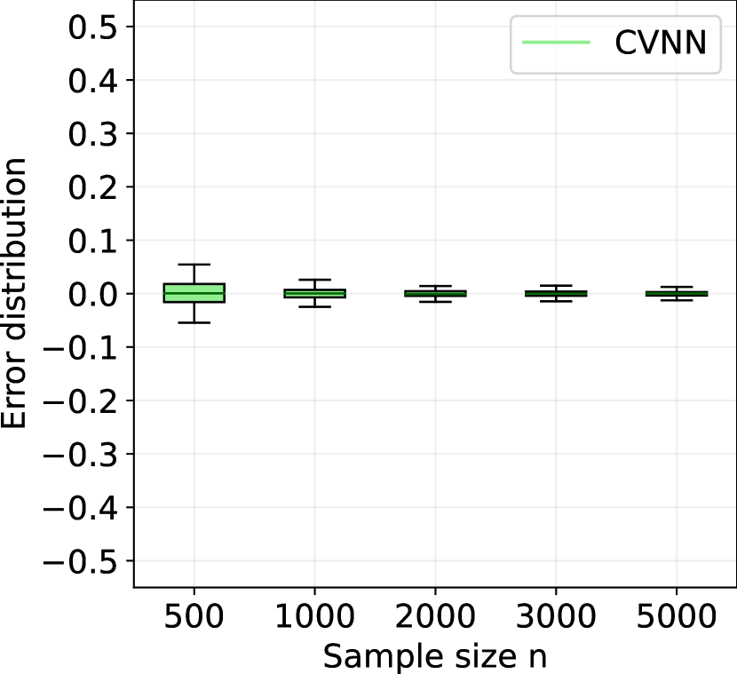
(b) “Up-In”, CVNN

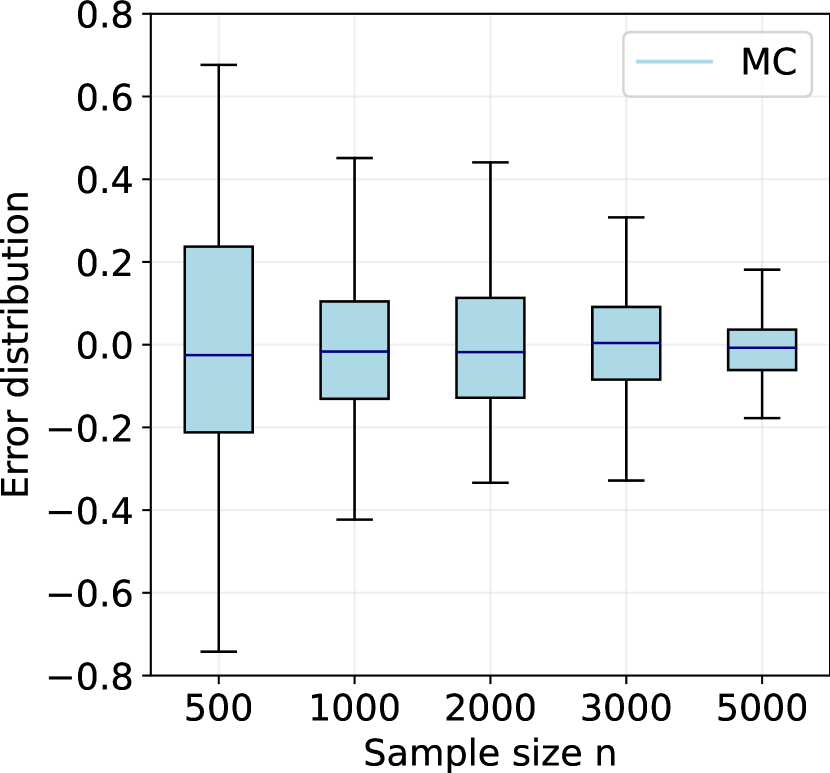
(c) “Up-Out”, MC

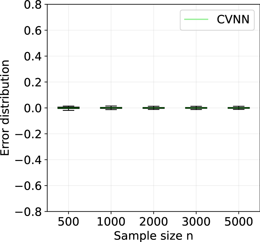
(d) “Up-Out”, CVNN

Figure 6: Barrier option pricing under Black–Scholes model with spot price $S_{0}=100$, strike $K=S_{0}$, maturity $T=2$ months, risk-free rate $r=0.1$, constant volatility $\sigma=0.3$, barrier price $H=130$. The boxplots are obtained over $100$ replications.

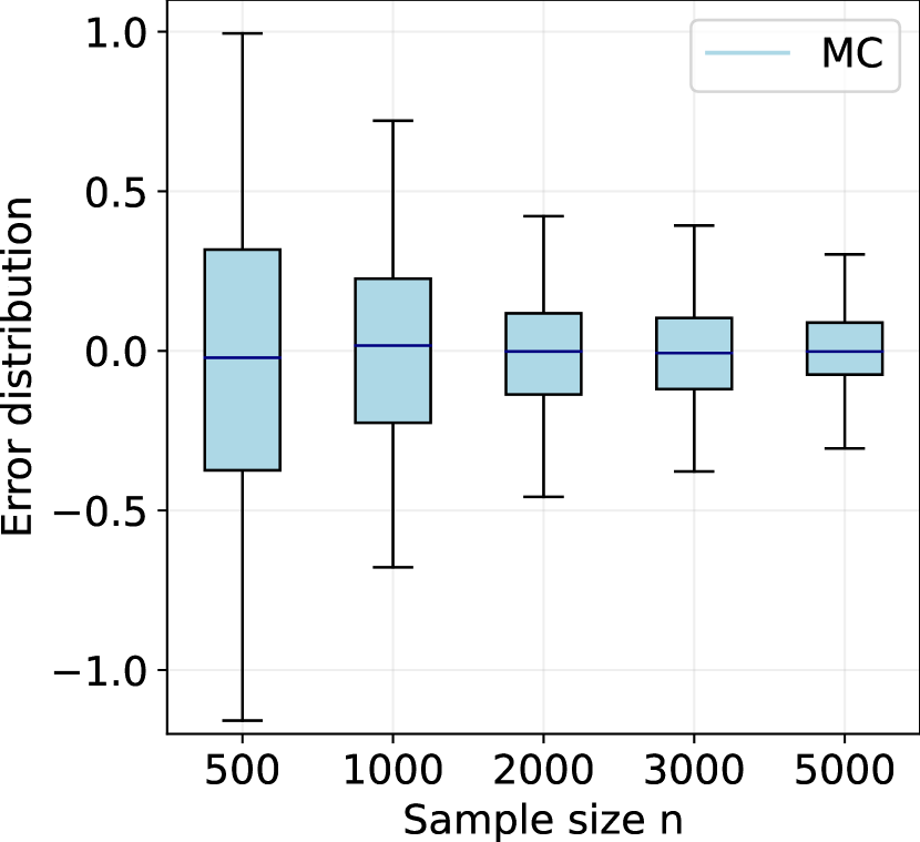
(a) “Up-In”, MC

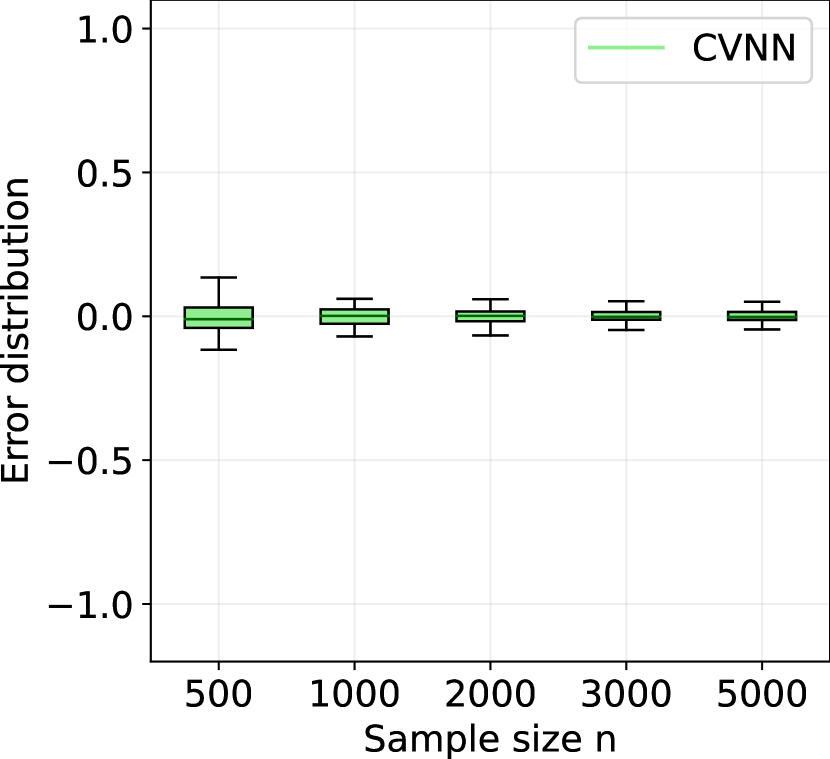
(b) “Up-In”, CVNN

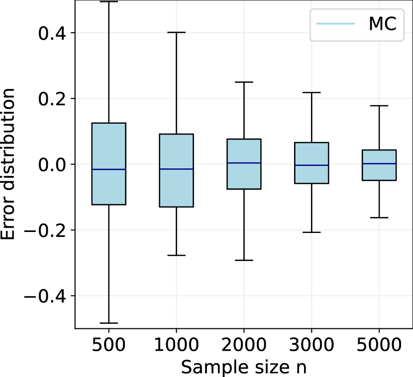
(c) “Up-Out”, MC

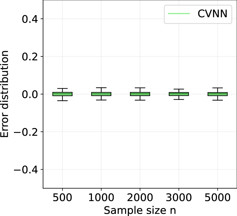
(d) “Up-Out”, CVNN

Figure 7: Boxplots of barrier option pricing with Heston Model with spot price $S_{0}=100$, strike $K=S_{0}$, barrier price $H=130$, maturity $T=2$ months, risk-free rate $r=0.1$, initial volatility $v_{0}=0.1$, long-run average variance $\theta=0.02$, rate of mean reversion $\kappa=4$, instantaneous correlation $\rho=0.8$ and volatility of volatility $\xi=0.9$. The boxplots are obtained over $100$ replications.

Results. Figure 6 shows the error distribution of the different Monte Carlo estimates (naive MC and CVNN) for the pricing of Barrier call options “up-in” and “up-out” in the Black–Scholes model. The boxplots are computed over $100$ independent replications and the true values of the options are approximated using the Python package QuantLib. Similarly, Figure 7 gathers the results for the Heston model. The variance is greatly reduced when using the control neighbors estimate compared to the standard Monte Carlo approach.

References

- Achddou et al. (2019) Juliette Achddou, Joseph Lam-Weil, Alexandra Carpentier, and Gilles Blanchard. A minimax near-optimal algorithm for adaptive rejection sampling. In Algorithmic Learning Theory, pages 94–126. PMLR, 2019.
- Audibert and Tsybakov (2007) J-Y. Audibert and A. B. Tsybakov. Fast learning rates for plug-in classifiers. Ann. Statist., 35(2):608–633, 2007.
- Barp et al. (2022) Alessandro Barp, Chris J Oates, Emilio Porcu, and Mark Girolami. A Riemann–Stein kernel method. Bernoulli, 28(4):2181–2208, 2022.
- Bentley (1975) Jon Louis Bentley. Multidimensional binary search trees used for associative searching. Communications of the ACM, 18(9):509–517, 1975.
- Biau and Devroye (2015) Gérard Biau and Luc Devroye. Lectures on the nearest neighbor method, volume 246. Springer, 2015.
- Black and Scholes (1973) Fischer Black and Myron Scholes. The pricing of options and corporate liabilities. Journal of political economy, 81(3):637–654, 1973.
- Bonneel et al. (2015) Nicolas Bonneel, Julien Rabin, Gabriel Peyré, and Hanspeter Pfister. Sliced and Radon Wasserstein barycenters of measures. Journal of Mathematical Imaging and Vision, 51:22–45, 2015.
- Caflisch (1998) Russel E Caflisch. Monte Carlo and quasi-Monte Carlo methods. Acta numerica, 7:1–49, 1998.
- Chopin and Gerber (2022) Nicolas Chopin and Mathieu Gerber. Higher-order stochastic integration through cubic stratification. arXiv preprint arXiv:2210.01554, 2022.
- Combes (2015) Richard Combes. An extension of McDiarmid’s inequality. arXiv preprint arXiv:1511.05240, 2015.
- Courty et al. (2017) Nicolas Courty, Rémi Flamary, Amaury Habrard, and Alain Rakotomamonjy. Joint distribution optimal transportation for domain adaptation. Advances in neural information processing systems, 30, 2017.
- Craven and Wahba (1978) Peter Craven and Grace Wahba. Smoothing noisy data with spline functions. Numerische Mathematik, 31(4):377–403, 1978.
- Cuturi (2013) Marco Cuturi. Sinkhorn distances: Lightspeed computation of optimal transport. Advances in neural information processing systems, 26, 2013.
- Doucet et al. (2001) Arnaud Doucet, Nando De Freitas, Neil James Gordon, et al. Sequential Monte Carlo methods in practice, volume 1. Springer, 2001.
- Evans and Swartz (2000) Michael Evans and Tim Swartz. Approximating integrals via Monte Carlo and deterministic methods. Oxford Statistical Science Series. Oxford University Press, Oxford, 2000.
- Friedman et al. (1977) Jerome H Friedman, Jon Louis Bentley, and Raphael Ari Finkel. An algorithm for finding best matches in logarithmic expected time. ACM Transactions on Mathematical Software (TOMS), 3(3):209–226, 1977.
- Gadat et al. (2016) Sébastien Gadat, Thierry Klein, and Clément Marteau. Classification in general finite dimensional spaces with the -nearest neighbor rule. Ann. Statist., 44(3):982–1009, 2016.
- Genevay et al. (2018) Aude Genevay, Gabriel Peyré, and Marco Cuturi. Learning generative models with Sinkhorn divergences. In International Conference on Artificial Intelligence and Statistics, pages 1608–1617. PMLR, 2018.
- Glasserman (2004) Paul Glasserman. Monte Carlo Methods in Financial Engineering, volume 53. Springer, 2004.
- Glynn and Szechtman (2002) Peter W Glynn and Roberto Szechtman. Some new perspectives on the method of control variates. In Monte Carlo and Quasi-Monte Carlo Methods 2000: Proceedings of a Conference held at Hong Kong Baptist University, Hong Kong SAR, China, November 27–December 1, 2000, pages 27–49. Springer, 2002.
- Gulrajani et al. (2017) Ishaan Gulrajani, Faruk Ahmed, Martin Arjovsky, Vincent Dumoulin, and Aaron C Courville. Improved training of Wasserstein GANs. Advances in neural information processing systems, 30, 2017.
- Haber (1966) Seymour Haber. A modified Monte-Carlo quadrature. Mathematics of Computation, 20(95):361–368, 1966.
- Haber (1967) Seymour Haber. A modified Monte-Carlo quadrature. II. Mathematics of Computation, 21(99):388–397, 1967.
- Haber (1969) Seymour Haber. Stochastic quadrature formulas. Mathematics of Computation, 23(108):751–764, 1969.
- Heston (1993) Steven L Heston. A closed-form solution for options with stochastic volatility with applications to bond and currency options. The review of financial studies, 6(2):327–343, 1993.
- Higdon et al. (2015) Dave Higdon, Jordan D McDonnell, Nicolas Schunck, Jason Sarich, and Stefan M Wild. A Bayesian approach for parameter estimation and prediction using a computationally intensive model. Journal of Physics G: Nuclear and Particle Physics, 42(3):034009, 2015.
- Hoff III et al. (1999) Kenneth E Hoff III, John Keyser, Ming Lin, Dinesh Manocha, and Tim Culver. Fast computation of generalized Voronoi diagrams using graphics hardware. In Proceedings of the 26th annual conference on Computer graphics and interactive techniques, pages 277–286, 1999.
- Hunter (2007) John D Hunter. Matplotlib: A 2d graphics environment. Computing in science & engineering, 9(03):90–95, 2007.
- Johnson et al. (2019) Jeff Johnson, Matthijs Douze, and Hervé Jégou. Billion-scale similarity search with GPUs. IEEE Transactions on Big Data, 7(3):535–547, 2019.
- Kabatyanskiı and Levenshteın (1974) GA Kabatyanskiı and VI Levenshteın. Bounds for packings on a sphere and in space. Problems of Information Transmission, 95:148–158, 1974.
- Kohler et al. (2006) Michael Kohler, Adam Krzyżak, and Harro Walk. Rates of convergence for partitioning and nearest neighbor regression estimates with unbounded data. Journal of Multivariate Analysis, 97(2):311–323, 2006.
- Kolouri et al. (2019) Soheil Kolouri, Kimia Nadjahi, Umut Simsekli, Roland Badeau, and Gustavo Rohde. Generalized sliced Wasserstein distances. Advances in neural information processing systems, 32, 2019.
- Leluc et al. (2021) R. Leluc, F. Portier, and J. Segers. Control variate selection for Monte Carlo integration. Statistics and Computing, 31, 07 2021. doi: 10.1007/s11222-021-10011-z.
- Merton (1973) Robert C Merton. Theory of rational option pricing. The Bell Journal of economics and management science, pages 141–183, 1973.
- Mezzadri (2007) Francesco Mezzadri. How to generate random matrices from the classical compact groups. Notices of the American Mathematical Society, 54(5):592–604, 2007.
- Nadjahi et al. (2021) Kimia Nadjahi, Alain Durmus, Pierre E Jacob, Roland Badeau, and Umut Simsekli. Fast approximation of the sliced-wasserstein distance using concentration of random projections. Advances in Neural Information Processing Systems, 34:12411–12424, 2021.
- Newton (1994) Nigel J Newton. Variance reduction for simulated diffusions. SIAM Journal on Applied Mathematics, 54(6):1780–1805, 1994.
- Novak (2016) Erich Novak. Some results on the complexity of numerical integration. In Monte Carlo and Quasi-Monte Carlo Methods, pages 161–183. Springer, 2016.
- Oates et al. (2017) Chris J Oates, Mark Girolami, and Nicolas Chopin. Control functionals for Monte Carlo integration. Journal of the Royal Statistical Society: Series B (Statistical Methodology), 79(3):695–718, 2017.
- Oates et al. (2019) Chris J Oates, Jon Cockayne, François-Xavier Briol, and Mark Girolami. Convergence rates for a class of estimators based on Stein’s method. Bernoulli, 25(2):1141–1159, 2019.
- Omohundro (1989) Stephen M Omohundro. Five balltree construction algorithms. International Computer Science Institute Berkeley, 1989.
- Pedregosa et al. (2011) Fabian Pedregosa, Gaël Varoquaux, Alexandre Gramfort, Vincent Michel, Bertrand Thirion, Olivier Grisel, Mathieu Blondel, Peter Prettenhofer, Ron Weiss, Vincent Dubourg, et al. Scikit-learn: Machine learning in Python. The Journal of Machine Learning Research, 12:2825–2830, 2011.
- Peyré et al. (2019) Gabriel Peyré, Marco Cuturi, et al. Computational optimal transport: With applications to data science. Foundations and Trends® in Machine Learning, 11(5-6):355–607, 2019.
- Portier and Segers (2019) F. Portier and J. Segers. Monte Carlo integration with a growing number of control variates. Journal of Applied Probability, 56(4):1168–1186, 2019. doi: 10.1017/jpr.2019.78.
- Portier (2023) François Portier. Nearest neighbor process: weak convergence and non-asymptotic bound. arXiv preprint arXiv:2110.15083, 2023.
- Rabin et al. (2012) Julien Rabin, Gabriel Peyré, Julie Delon, and Marc Bernot. Wasserstein barycenter and its application to texture mixing. In Scale Space and Variational Methods in Computer Vision: Third International Conference, SSVM 2011, Ein-Gedi, Israel, May 29–June 2, 2011, Revised Selected Papers 3, pages 435–446. Springer, 2012.
- Richards (1974) Frederic M Richards. The interpretation of protein structures: total volume, group volume distributions and packing density. Journal of Molecular Biology, 82(1):1–14, 1974.
- Rubinstein (1981) Reuven Y. Rubinstein. Simulation and the Monte Carlo method. John Wiley & Sons, Inc., New York, 1981.
- Rycroft (2009) Chris Rycroft. Voro++: A three-dimensional Voronoi cell library in C++. Technical report, Lawrence Berkeley National Lab.(LBNL), Berkeley, CA (United States), 2009.
- Sacks et al. (1989) Jerome Sacks, William J Welch, Toby J Mitchell, and Henry P Wynn. Design and analysis of computer experiments. Statistical science, 4(4):409–423, 1989.
- South et al. (2022) LF South, CJ Oates, A Mira, and C Drovandi. Regularized zero-variance control variates. Bayesian Analysis, 1(1):1–24, 2022.
- Stone (1974) Mervyn Stone. Cross-validatory choice and assessment of statistical predictions. Journal of the royal statistical society: Series B (Methodological), 36(2):111–133, 1974.
- Toscano-Palmerin and Frazier (2022) Saul Toscano-Palmerin and Peter I Frazier. Bayesian optimization with expensive integrands. SIAM Journal on Optimization, 32(2):417–444, 2022.
- Villani (2009) Cédric Villani. Optimal transport: Old and New, volume 338. Springer, 2009.
- Virtanen et al. (2020) Pauli Virtanen, Ralf Gommers, Travis E Oliphant, Matt Haberland, Tyler Reddy, David Cournapeau, Evgeni Burovski, Pearu Peterson, Warren Weckesser, Jonathan Bright, et al. SciPy 1.0: fundamental algorithms for scientific computing in Python. Nature methods, 17(3):261–272, 2020.
- Zeger and Gersho (1994) Kenneth Zeger and Allen Gersho. Number of nearest neighbors in a Euclidean code. IEEE Transactions on Information Theory, 40(5):1647–1649, 1994.