Shape Formation and Locomotion with Joint Movements in the Amoebot Model

Abstract

We are considering the geometric amoebot model where a set of $n$ amoebots is placed on the triangular grid. An amoebot is able to send information to its neighbors, and to move via expansions and contractions. Since amoebots and information can only travel node by node, most problems have a natural lower bound of $\Omega(D)$ where $D$ denotes the diameter of the structure. Inspired by the nervous and muscular system, Feldmann et al. have proposed the reconfigurable circuit extension and the joint movement extension of the amoebot model with the goal of breaking this lower bound.

In the joint movement extension, the way amoebots move is altered. Amoebots become able to push and pull other amoebots. Feldmann et al. demonstrated the power of joint movements by transforming a line of amoebots into a rhombus within $O(\log n)$ rounds. However, they left the details of the extension open. The goal of this paper is therefore to formalize and extend the joint movement extension. In order to provide a proof of concept for the extension, we consider two fundamental problems of modular robot systems: shape formation and locomotion.

We approach these problems by defining meta-modules of rhombical and hexagonal shape, respectively. The meta-modules are capable of movement primitives like sliding, rotating, and tunneling. This allows us to simulate shape formation algorithms of various modular robot systems. Finally, we construct three amoebot structures capable of locomotion by rolling, crawling, and walking, respectively.

1 Introduction

Programmable matter consists of homogeneous nano-robots that are able to change the properties of the matter in a programmable fashion, e.g., the shape, the color, or the density [55]. We are considering the geometric amoebot model [14, 15, 16] where a set of $n$ nano-robots (called amoebots) is placed on the triangular grid. An amoebot is able to send information to its neighbors, and to move by first expanding into an unoccupied adjacent node, and then contracting into that node. Since amoebots and information can only travel node by node, most problems have a natural lower bound of $\Omega(D)$ where $D$ denotes the diameter of the structure. Inspired by the nervous and muscular system, Feldmann et al. [23] proposed the reconfigurable circuit extension and the joint movement extension with the goal of breaking this lower bound.

In the reconfigurable circuit extension, the amoebot structure is able to interconnect amoebots by circuits. Each amoebot can send a primitive signal on circuits it is connected to. The signal is received by all amoebots connected to the same circuit. Among others, Feldmann et al. [23] solved the leader election problem, compass alignment problem, and chirality agreement problem within $O(\log n)$ rounds w.h.p. These problems will be important to coordinate the joint movements. Afterwards, Padalkin et al. [45] explored the structural power of the circuits by considering the spanning tree problem and symmetry detection problem. Both problems can be solved within polylogarithmic time w.h.p.

In the joint movement extension, the way amoebots move is altered. In a nutshell, an expanding amoebot is capable of pushing other amoebots away from it, and a contracting amoebot is capable of pulling other amoebots towards it. Feldmann et al. [23] demonstrated the power of joint movements by transforming a line of amoebots into a rhombus within $O(\log n)$ rounds. However, they left the details of the extension open. The goal of this paper is therefore to formalize and extend the joint movement extension. In order to provide a proof of concept for the extension, we consider two fundamental problems of modular robot systems (MRS): shape formation and locomotion. We study these problems from a centralized view to explore the limits of the extension.

In the shape formation problem, an MRS has to reconfigure its structure into a given shape. Examples for shape formation algorithms in the original amoebot model can be found in [17, 18, 35, 40]. However, all of these are subject of the aforementioned natural lower bound. To our knowledge, polylogarithmic time solutions were found for two types of MRSs: in the nubot model [60] and crystalline atom model [6]. We will show that in the joint movement extension, the amoebots are able to simulate the shape formation algorithm for the crystalline atom model, and with that break the lower bound.

In the locomotion problem, an MRS has to move along an even surface as fast as possible. We might also ask the MRS to transport an object along the way. In the original amoebot model, one would use the spanning tree primitive to move along the surface [14]. However, we only obtain a constant velocity with that. Furthermore, the original amoebot model does not allow us to transport any objects. In terrestrial environments, there are three basic types of locomotion: rolling, crawling, and walking [26, 33]. For each of these locomotion types, we will present an amoebot structure.

2 Preliminaries

In this section, we introduce the geometric amoebot model [15, 16] and formalize the joint movement extension.

2.1 Geometric Amoebot Model

In the geometric amoebot model [15], a set of $n$ amoebots is placed on the infinite regular triangular grid graph $G_{\Delta}=(V,E)$ (see Figure 1(a)). An amoebot is an anonymous, randomized finite state machine that either occupies one or two adjacent nodes of $G_{\Delta}$, and every node of $G_{\Delta}$ is occupied by at most one amoebot. If an amoebot occupies just one node, it is called contracted (a single node) and otherwise expanded (two nodes connected by a black edge). Two amoebots that occupy adjacent nodes in $G_{\Delta}$ are connected by bonds (red edges). An amoebot can move through contractions and expansions (see Figure 2). We refer to [15] for more details.

(a) Triangular grid.

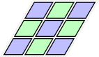
(b) Rhombical tesselation.

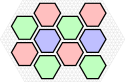
(c) Hexagonal tesselation.

Figure 1: Domains. The figures show the domains we are working with. The tesselations will be explained in Section 3. Note that there are spaces between the meta-modules since a node cannot be occupied by more than one amoebot. However, the spaces do not contain any nodes.

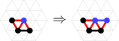
(a) Expansion.

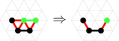
(b) Contraction.

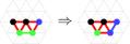
(c) Handover.

Figure 2: Movements in the classical model. Red lines indicate bonds. Blue amoebots are expanding. Green amoebots are contracting. (a) An expanded amoebot occupying nodes $v$ and $w$ can contract into one of its occupied nodes. Thereafter, it only occupies that node. (b) A contracted amoebot occupying node $u$ can expand into an unoccupied adjacent node $v$. Thereafter, it occupies both, $u$ and $v$. (c) Two adjacent amoebots can perform a handover if one is contracted and the other is expanded: let node $u$ be occupied by the contracted amoebot, and let nodes $v$ and $w$ be occupied by the expanded amoebot such that nodes $u$ and $v$ are adjacent. The contracted amoebot expands into node $v$ while the expanded node contracts into node $w$.

Let the amoebot structure $S\subseteq V$ be the set of nodes occupied by the amoebots. We say that $S$ is connected iff $G_{S}$ is connected, where $G_{S}=G_{\Delta}|_{S}$ is the graph induced by $S$. Initially, $S$ is connected. Also, we assume the fully synchronous activation model, i.e., the time is divided into synchronous rounds, and every amoebot is active in each round. We justify this assumption with the reconfigurable circuit extension. On activation, each amoebot may perform a movement and update its state as a function of its previous state. However, if an amoebot fails to perform its movement, it remains in its previous state. The time complexity of an algorithm is measured by the number of synchronized rounds required by it.

2.2 Joint Movement Extension

In the joint movement extension [23], the way the amoebots move is altered. The idea behind the extension is to allow amoebots to push and pull other amoebots. The necessary coordination of such movements can be provided by the reconfigurable circuit extension. Since we study the problems from a centralized view, we refrain from describing that extension and refer to [23, 45]. In the following, we formalize the joint movement extension. Joint movements are performed in two steps.

In the first step, the amoebots remove bonds from $G_{S}$ as follows. Each amoebot can decide to release an arbitrary subset of its currently incident bonds in $G_{S}$. A bond is removed iff either of the amoebots at the endpoints releases the bond. However, an expanded amoebot cannot release the bond connecting its occupied nodes. Let $E_{R}\subseteq E_{S}$ denote the set of the remaining bonds, and $G_{R}=(S,E_{R})$ the resulting graph. We require that $G_{R}$ is connected since otherwise, disconnected parts might float apart. We say that a connectivity conflict occurs iff $G_{R}$ is not connected. Whenever a connectivity conflict occurs, the amoebot structure transitions into an undefined state such that we become unable to make any statements about the structure.

In the second step, each amoebot may perform one of the following movements within the time period $[0,1]$. A contracted amoebot may expand on one of the axes as follows (see Figure 3(a)). At $t=0$, the amoebot splits its single node into two nodes, adds a bond between them, and assigns each of its other incident bonds to one of the resulting nodes. Then, the amoebot uniformly extends the length of the new bond. At $t\in[0,1]$, that bond has a length of $t$. In the process, the incident bonds do not change their orientations or lengths.

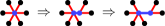
(a) Expansion.

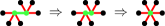
(b) Contraction.

(c) Handover.

Figure 3: Movements in the extension. Red lines indicate bonds. Blue amoebots are expanding. Green amoebots are contracting. The first two figures show a movement in $0.5$ time steps.

An expanded amoebot may contract into a single node as follows (see Figure 3(b)). The amoebot uniformly reduces the length of the bond between its endpoints. At $t\in[0,1]$, the bond has a length of $1-t$. At $t=1$, the amoebot removes that bond, fuses its endpoints into a single node, and assigns all of its other incident bonds to the resulting node. In the process, the incident bonds do not change their orientations or lengths. We remove duplicates of bonds if any occur (see Figure 4(a)).

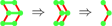
(a) Duplicates.

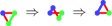
(b) Collision.

Figure 4: Special cases. Red lines indicate bonds. Blue amoebots are expanding. Green amoebots are contracting. Each figure shows a movement in $0.5$ time steps.

Furthermore, a contracted amoebot $x$ occupying node $u$ and an expanded amoebot $y$ occupying nodes $v$ and $w$ may perform a handover if there is a bond $b$ between $u$ and $v$, as follows (see Figure 3(c)). At an arbitrary $t\in[0,1]$, we flip $b=\{u,v\}$ and $\{v,w\}$ such that $x$ becomes an expanded amoebot occupying nodes $u$ and $v$, $y$ becomes a contracted amoebot occupying $w$, and $b$ becomes $\{v,w\}$. We have to include the handover to ensure universality of the model since otherwise, it would not be possible to move through a narrow tunnel. In theory, all movement primitives presented in Section 3 can be realized without handovers. However, for reasons of clarity and comprehensibility, we will still make use of the handovers.

The amoebots may not be able to perform their movements. We distinguish between two cases. First, the amoebots may not be able to perform their movements while maintaining their relative positions (see Figure 5(a)). We call that a structural conflict. Second, parts of the structure may collide into each other. More precisely, a collision occurs if there is a $t\in[0,1]$ such that two non-adjacent bonds intersect at some point (see Figure 5(b)). In particular, note that an expanded amoebot cannot contract if it has two incident bonds to the same node even if the amoebot occupying that node expands at the same time without causing a collision (see Figure 4(b)). Whenever either a structural conflict or a collision occurs, the amoebot structure transitions into an undefined state such that we become unable to make any statements about the structure.

Otherwise, at $t=1$, we obtain a graph $G_{M}=(S,E_{M})$ that can be mapped on the triangular grid $G_{\Delta}$ (see Figure 5(a)). Since $G_{R}$ is connected, the mapping of $G_{M}$ is unique except for translations (if one exists). We choose any mapping as our next amoebot structure. Afterwards, the amoebots reestablish all possible bonds. Unless stated otherwise, each arrow in the figures indicates a single round. The left side shows the structure after the removal of bonds (first step), and the right side the structure after the execution of movements (second step). We chain multiple rounds if we do not change bonds.

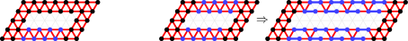
(a) Structural conflicts and mappings. In the left figure, the expansions cause a structural conflict. In the right figure, the amoebot structure can be mapped onto the triangular grid after the movement.

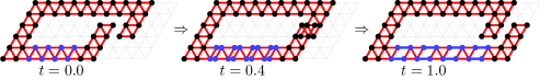
(b) Collision. Initially, we have a valid amoebot structure given ($t=0$). The resulting amoebot structure can be mapped on $G_{\Delta}$ ($t=1$). However, for $t\in[0.25,0.75]$, parts of the structure collide.

Figure 5: Joint movements. Red lines indicate bonds. Blue amoebots are expanding.

We assume that the joint movements are performed within look-compute-move cycles. In the look phase, each amoebot observes its neighborhood and receives signals (beeps) from other amoebots, according to the reconfigurable circuit structure of the system. In the compute phase, each amoebot may perform computations, change its state, and decide the actions to perform in the next phase (i.e., which bonds to release, and which movement to perform). In the move phase, each amoebot may release an arbitrary subset of its incident bonds, and perform a movement.

2.3 Problem Statement and Our Contribution

In this paper, we formalize and extend the joint movement extension proposed by Feldmann et al. [23]. In the following, we provide a proof of concept. For that, we focus on two fundamental problems of MRSs: shape formation and locomotion. We study these problems from a centralized view to explore the limits of the extension.

In the shape formation problem, an MRS has to reconfigure its structure into a given shape. For that, we define meta-modules of rhombical and hexagonal shape. We show that these meta-modules are able to perform various movement primitives of other MRSs, e.g., crystalline atoms, and rectangular/hexagonal metamorphic robots. This allows us to simulate the shape formation algorithms of those models.

In the locomotion problem, an MRS has to move along an even surface as fast as possible. We might also ask the MRS to transport an object along the way. We present three amoebot structures that are able to move by rolling, crawling, and walking, respectively. We analyze their velocities and compare them to other structures of similar models.

2.4 Related Work

MRSs can be classified into various types, e.g., lattice-type, chain-type, and mobile-type [1, 9, 64, 65]. We refer to the cited papers for examples. We will focus on lattice-type MRSs. These in turn can be characterized by three properties: (i) the lattice, (ii) the connectivity constraint, and (iii) the allowed movement primitives [2].

Various MRSs have been defined for different lattices, e.g., [12, 60] utilize the triangular grid, and [3, 22, 49] utilize the Cartesian grid. We will build meta-modules for the Cartesian and hexagonal grid. Note that some MRSs were also physically realized. Examples for MRSs using the triangular grid are hexagonal metamorphic robots [12], HexBots [50], fractal machines [42], and catoms [34]. Examples for MRSs using the Cartesian grid are CHOBIE II [54], EM-Cubes [7], M-Blocks [47], pneumetic celluar robots [28], and XBots [59].

We can identify four types of connectivity constraints: (i) the structure is connected at all times, (ii) the structure is connected except for moving robots, (iii) the structure is connected before and after movements, and (iv) there are no connectivity constraints. Our joint movement extension falls into the first category. Other examples are crystalline atoms [48], telecubes [53, 57], and prismatic cubes [58]. Examples for the second category are the sliding cube model [10, 24], rectangular [22] and hexagonal metamorphic robots [12], and for the third category the nubot model [60] and the line pushing model [3]. An example for the last category is the variant of the amoebot model considered by Dufoulon et al. [21].

The most common movement primitives for MRSs on the Cartesian grid are the rotation and slide primitives (see Figures 6(b) and 6(c)), and for MRSs on the triangular grid the rotation primitive (see Figure 6(a)). Some models may constrain these movement primitives (see Figure 7). We refer to [2, 27] for a deeper discussion about possible constraints. One way to bypass such constraints is to construct meta-modules, e.g., see [19, 27, 43]. Our meta-modules implement all aforementioned movement primitives without any constraints, i.e., they perform them in place.

(a) Rotation primitive.

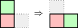
(b) Rotation primitive.

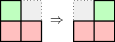
(c) Slide primitive.

(d) Contraction primitive.

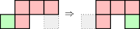
(e) Tunnel primitive.

Figure 6: Examples of movement primitives. The green modules are moving, respectively. Models that utilize the Cartesian grid usually assume square modules. In Section 3.1, we utilize rhombical modules instead.

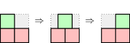
(a) Sliding model, e.g., [27].

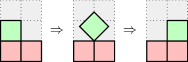
(b) Pivoting model, e.g., [2].

Figure 7: Constrained movement primitives. The green modules are moving, respectively. The gray cells must be empty. Both primitives have the same result while the pivoting model requires more free space than the sliding model.

From all aforementioned models, crystalline atoms [48], telecubes [53, 57], and prismatic cubes [58] are the closest to our joint movement extension. In these MRSs, each robot has the shape of a unit square and is able to expand an arm from each side by half a unit. Adjacent robots are able to attach and detach their arms. Similar to our joint movement extension, a robot can move attached robots by expanding or contracting its arms. In contrast to amoebots, a line of robots cannot reconfigure to any other shape since each pair of robots can only have a single point of contact [5]. In order to allow arbitrary shape formations, the robots are combined into meta-modules of square shape that are capable of various movement primitives, e.g., the rotation, slide, contraction, and tunnel primitives (see Figures 6(b), 6(d), 6(c) and 6(e)). Our rhombical meta-modules can implement all these movement primitives. The rhombical shape has two advantages compared to the square shape. First, we can implement further movement primitives that provide us with a simple way to construct a walking structure. Second, we can utilize rhombical meta-modules as a basis for hexagonal meta-modules.

3 Meta-Modules

In this section, we will combine multiple amoebots to meta-modules. In other models for programmable matter and modular robots, meta-modules have proven to be very useful. For example, they allow us to bypass restrictions on the reconfigurability [19, 56] and to simulate (shape formation) algorithms for other models [4, 46].

In the first two subsections, we will present meta-modules of rhombical and hexagonal shape, respectively. In the third and fourth subsection, we discuss how to increase the stability of the structure during the movements, and how to construct rhombical and hexagonal meta-modules from an arbitrary amoebot structure.

3.1 Rhombical Meta-Modules

Let $\ell$ be a positive even integer. Our rhombical meta-module consists of $\ell^{2}/2$ uniformly oriented expanded amoebots that we arrange into a rhombus of side length $\ell-1$ (see Figure 8). We obtain a parallelogram of side lengths $\ell-1$ and $\ell/2-1$ if we contract all amoebots (see Figure 8(a)). Note that we have to remove some bonds to perform the contraction. We can expand the parallelogram again by reversing the contractions.

Lemma 3.1.

Our implementation of the contraction and expansion primitive requires a single round, respectively.

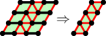
(a) Contraction primitive.

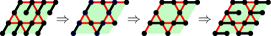
(b) Reorientation primitive.

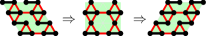
(c) Realignment primitive.

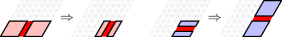
(d) Rotation primitive.

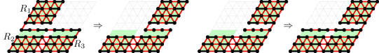
(e) Slide primitive.

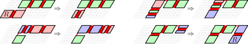
(f) $k$-tunnel primitive.

Figure 8: Movement primitives for rhombical meta-modules. Red meta-modules perform a pull operation, and blue meta-modules a push operation.

There are exactly two possibilities to arrange the uniformly oriented expanded amoebots in a rhombus. By reorienting the amoebots in pairs with the help of handovers, we can reorientate all amoebots within a rhombus (see Figure 8(b)).

Lemma 3.2.

Our implementation of the reorientation primitive requires $3$ rounds.

Furthermore, there are three possibilities to align the sides of a rhombus to the axes of the triangular grid. By sliding each second row along its axis to the other side, we can realign the other axis a rhombus is aligned to (see Figure 8(c)). Note that in combination with the reorientation of the amoebots within a rhombus, we are able to align a rhombus with any two axes of the triangular grid.

Lemma 3.3.

Our implementation of the realignment primitive requires $2$ rounds.

We can arrange the meta-modules on a rhombical tesselation of the plane if they are all aligned to the same axes (see Figure 1(b)). Note that due to the triangular grid, the meta-modules are not connected diagonally everywhere. Hence, we will only consider meta-modules connected if their sides are connected. In the following, we introduce two movement primitives: the slide and $k$-tunnel primitive. Our implementations of these primitives are similar to the ones for crystalline robots (e.g., [5]) and teletubes (e.g., [57]).

In the slide primitive, we move a meta-module $R_{1}$ along two adjacent substrate meta-modules $R_{2}$ and $R_{3}$ (see Figure 6(c)). We realize the primitive as follows (see Figure 8(e)). We assume that all amoebots are orientated into the movement direction. Otherwise, we apply the reorientation primitive. With respect to Figure 8(e), let $L_{1}$ denote the uppermost layer of $R_{2}$ and $R_{3}$, and $L_{2}$ the second uppermost layer of $R_{2}$ and $R_{3}$. Our slide primitive consists of two rounds. In the first round, we contract all amoebots in $L_{1}$ after removing all bonds between $L_{1}$ and $R_{1}$ except the last one in the movement direction, and all bonds between $L_{1}$ and $L_{2}$ except the last one in the opposite direction. This moves $R_{1}$ into its target position. In the second round, we restore $R_{2}$ and $R_{3}$. For that, we expand $L_{1}$ again after removing all bonds between $L_{1}$ and $R_{1}$, and between $L_{1}$ and $L_{2}$ except the last ones in the movement direction, respectively. This ensures that $R_{1}$ stays in place.

Lemma 3.4.

Our implementation of the slide primitive requires $2$ rounds.

In the $k$-tunnel primitive, we move a meta-module $R$ through a simple path of meta-modules with $k$ corners to the other end (see Figure 6(e)). However, we do not move $R$ directly through the path. Instead, we make use of the following two basic operations. First, by contracting two adjacent meta-modules into parallelograms, we pull one meta-module into the other (see the first round in Figure 8(f)). Second, by expanding two adjacent contracted meta-modules, we push one meta-module out again (see the fourth round in Figure 8(f)).

Now, consider a line of at least 4 meta-modules with two contracted meta-modules at one end. By expanding those two meta-modules and contracting the two meta-modules at the other end, we transfer a meta-module from one end to the other end without changing the length of the line (see the third round in Figure 8(f)). If we have only a line of 3 meta-modules, it suffices to contract and expand one meta-module, respectively (see the second round in Figure 8(f)). Note that we have to remove most of the bonds along the line to permit the line to move freely. The pull and push operations allow us to transfer $R$ from one corner to the next corner in a single round.

Lemma 3.5.

Our implementation of the $k$-tunnel primitive requires $k+1$ rounds.

In particular, note that a $1$-tunnel allows us to move a meta-module around another one (see Figure 8(d)). In other models for modular robot systems, this simple case is known as the rotation primitive.

Lemma 3.6.

Our implementation of the rotation primitive requires $2$ rounds.

Akitaya et al. [2] have introduced two further movement primitives for rectangular MRSs: the leapfrog and the monkey (see Figure 9). In these primitives, the moving module performs a ‘jump’ between two not adjacent modules. We are able to transfer these primitives to our rhombical meta-modules. The idea is to divide the meta-modules into submodules to bridge the gap between the start and target position of the moving meta-module (see Figure 10).

Lemma 3.7.

Our implementation of the leapfrog and monkey primitives requires $O(1)$ rounds, respectively.

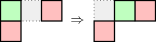
(a) Leapfrog jump.

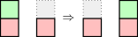
(b) Straight monkey jump.

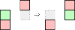
(c) Diagonal monkey jumps.

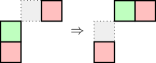
Figure 9: Leapfrog and monkey jumps. These movement primitives were introduced by Akitaya et al. [2]. We can simulate these by dividing the meta-modules into submodules. With these, we build a bridge to the new position of the meta-module by applying slide and $k$-tunnel primitives.

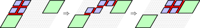
(a) Leapfrog jump.

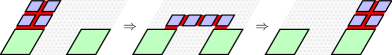
(b) Straight monkey jump.

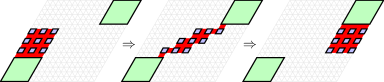
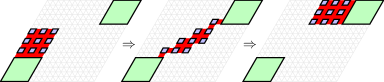
(c) Diagonal monkey jumps.

Figure 10: Leapfrog and monkey jumps. These movement primitives were introduced by Akitaya et al. [2]. We can simulate these by dividing the meta-modules into submodules. With these, we build a bridge to the new position of the meta-module by applying slide and $k$-tunnel primitives.

3.2 Hexagonal Meta-Modules

Let $\ell$ be an even integer as before. Our hexagonal meta-module consists of three rhombical meta-modules of side length $\ell-1$ (see Figure 11(a)). We arrange them into a hexagon of alternating side lengths $\ell$ and $\ell-1$.

There are two possibilities to arrange the rhombical meta-modules in the hexagon (see Figure 11(a)). We can switch between them as follows. The hexagonal meta-module can be split into three equilateral triangles of side length $\ell-1$, and three equilateral triangles of side length $\ell-2$. The idea is to apply a similar technique as in the realignment primitive for rhombical meta-modules. In the first round, each second row contracts but without shifting the other rows. In the second round, the rhombi interchange the smaller triangles through handovers. In the third round, we expand the contracted amoebots into the opposite direction – again without shifting the other rows.

Lemma 3.8.

Our implementation of the switching primitive requires $3$ rounds.

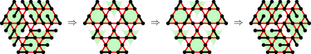
(a) Switching primitive.

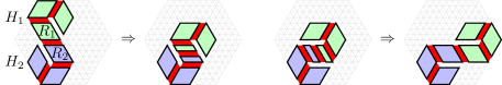
(b) Rotation primitive.

Figure 11: Movement primitives for hexagonal meta-modules.

We can arrange the meta-modules on a hexagonal tesselation of the plane (see Figure 1(c)). In the following, we introduce the rotation primitive for hexagonal meta-modules.

In the rotation primitive, we move a hexagonal meta-module $H_{1}$ around another hexagonal meta-module $H_{2}$ as follows (see Figure 11(b)). We arrange $H_{2}$ such that a rhombical meta-module $R_{2}$ is adjacent to both the old and new position of $H_{1}$, and $H_{1}$ such that the rhombical meta-module $R_{1}$ adjacent to $R_{2}$ is aligned to the same axes as $R_{2}$. We contract $R_{1}$ and $R_{2}$, and then expand them into the direction of the new position of $H_{1}$ (compare to Section 3.1). This movement primitive requires two rounds. Note that additional steps may be necessary to switch or reorientate the rhombical meta-modules beforehand.

Lemma 3.9.

Our implementation of the rotation primitive requires $2$ rounds.

3.3 Stability

One might argue that removing too many bonds may destabilize the structure during the movements. It is therefore desirable to maintain the connectivity between the amoebots as much as possible. Ideally, we want to only remove a constant fraction of all incident bonds of a connected component. Formally, let $\Gamma_{G}(U)=\{\{u,v\}\in E\mid u\in U\land v\not\in U\}$ where $G=(V,E)$. For each connected component $U\subseteq S$, we require $|\Gamma_{G_{R}}(U)|=\Theta(|\Gamma_{G_{S}}(U)|)$. This already holds for all presented movement primitives except for the slide and $k$-tunnel primitives of rhombical meta-modules. In the following, we present alternative implementations that increase the connectivity for these primitives.

First, consider the slide primitive. Recall that we need to slide a meta-module $R_{1}$ along two meta-modules $R_{2}$ and $R_{3}$ (see Figure 6(c)). We refer to Section 3.1 for details. The idea is to enlarge the moving part as follows (see Figure 12). For the sake of simplicity, we assume that $\ell$ is divisible by $8$. We partition $R_{2}$ and $R_{3}$ into $4\times 4$ submodules, respectively. The slide primitive consists of the following three rounds. In the first round, we utilize the submodules adjacent to the start and target position of $R_{1}$ to move $R_{1}$ to the center position. In the second round, we restore $R_{2}$ and $R_{3}$ again. In the last two rounds, we mirror the first two rounds to move $R_{1}$ to its target position.

Lemma 3.10.

Our alternative implementation of the slide primitive requires $3$ rounds.

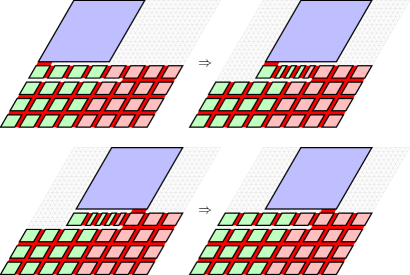
Figure 12: Slide primitive with a higher expansion. The rhombi indicate the meta-modules. The blue rhombi indicate $R_{1}$, and the green and red rhombi indicate $R_{2}$ and $R_{3}$, respectively. The red color between the meta-modules indicate bonds.

Second, consider the $k$-tunnel primitive. Recall that we need to move a meta-module $R$ through a simple path of meta-modules with $k$ corners to the other end (see Figure 6(e)). We refer to Section 3.1 for details.

We now discuss how to perform a single step of the $k$-tunnel, i.e., how to transfer a meta-module between two corners. Consider the line of meta-modules between those corners. One end contains two contracted meta-modules. We distinguish between to cases: (i) there is at least one other meta-module between the corners (see Figure 13), and (ii) there is no other meta-module between the corners (see Figure 14).

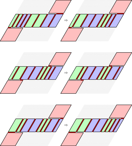
Figure 13: First case for the $k$-tunnel primitive. The rhombi and parallelograms indicate the meta-modules and submodules, respectively. Adjacent parallelograms of the same color belong to the same meta-module. The green and blue parallelograms indicate the considered line of meta-modules. The red color between the meta-modules indicate bonds.

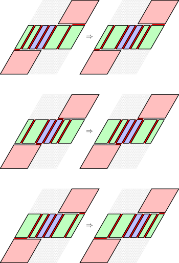
Figure 14: Second case for the $k$-tunnel primitive. The rhombi and parallelograms indicate the meta-modules and submodules, respectively. Adjacent parallelograms of the same color belong to the same meta-module. The green and blue parallelograms indicate the considered line of meta-modules. The red color between the meta-modules indicate bonds.

For the sake of simplicity, we assume that $\ell$ is divisible by $4$. We divide each meta-module of the line into two submodules orthogonally to the movement direction. Each submodule forms a parallelograms of side lengths $\ell-1$ and $\ell/2-1$. We assume that all expanded amoebots are orientated into the movement direction. This allows us to contract the submodules into parallelograms of side lengths $\ell-1$ and $\ell/4-1$.

The difficulty lies in maintaining enough bonds to the meta-modules attached to the corners. We will ensure that there is always a submodule that maintains its bonds. A single step of the $k$-tunnel primitive consists of the following three rounds.

In the first round, we contract or expand all submodules that we would have in the original version of the $k$-tunnel primitive – except for the ones at the two ends of the line. We use those two to maintain the bonds to attached meta-modules. Note that if we maintained the bonds at other submodules, we would move the line.

In the second round, we swap the states of the submodules of the meta-module at both ends. We use the third submodule of both ends to maintain the bonds to attached meta-modules. In the third round, we complete the transfer by contracting and expanding the remaining two submodules. We use the submodules at the two ends of the line again to maintain the bonds to attached meta-modules.

Lemma 3.11.

Our alternative implementation of the $k$-tunnel primitive requires $3\cdot(k+1)$ rounds.

3.4 Meta-Module Construction

So far, we have considered amoebot structures that are already composed of rhombical and hexagonal meta-modules. However, the initial amoebot structure may be arbitrary. In this section, we consider the transformation of a line of amoebots to a line of rhombical and hexagonal meta-modules, respectively. The formation of a line of amoebots from an arbitrary amoebot structure has been considered in previous work (e.g., [40]).

First, we form a line of $r$ rhombical meta-modules of side length $\ell-1$ from a line of $n=r\cdot\ell^{2}/2$ amoebots as follows (see Figure 15(a)). For that, we divide the line of amoebots into groups of $\ell$ amoebots and apply the following procedure introduced by Feldmann et al. [23] on each group of amoebots. The amoebots expand such that the height is doubled. Next, we reorientate the amoebots using handovers. Then, the amoebots contract again such that the width is halved. Thus, each iteration of the procedure doubles the height and halves the width. We repeat this procedure until the width is 1. Clearly, we need $O(\log\ell)$ iterations. Each iteration requires $O(1)$ rounds. Overall, the procedure requires $O(\log\ell)$ rounds. At the end of the second step, we obtain a parallelogram of side length $\ell-1$ and $r\cdot\ell/2-1$ filled with contracted amoebots. It remains to expand all amoebots to obtain the line of $r$ rhombical meta-modules. We obtain the following theorem.

Theorem 3.12.

There is a centralized algorithm that forms a line of $r$ rhombical meta-modules of side length $\ell-1$ from a line of $n=r\cdot\ell^{2}/2$ amoebots within $O(\log n)$ rounds.

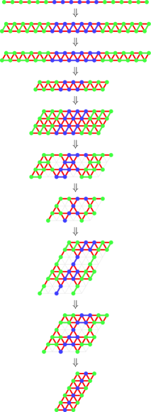
(a) Rhombical meta-modules.

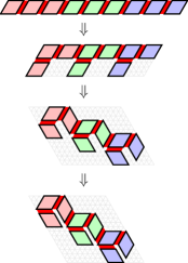
(b) Hexagonal meta-modules.

Figure 15: Construction of meta-modules. Adjacent amoebots and meta-modules of the same color belong to the same group, respectively.

Second, we form a line of $h=\frac{r}{3}$ hexagonal meta-modules of alternating side lengths $\ell$ and $\ell-1$ from a line of $r$ rhombical meta-modules of side length $\ell-1$ as follows (see Figure 15(b)). At the start, we divide the line of rhombical meta-modules into groups of $3$ rhombical meta-modules and apply the following three steps to each group. In the first step, we apply the $k$-tunnel primitive to move the first meta-module through the second meta-module. In the second step, we apply the realignment primitive on the first and third meta-module. In the third step, we apply the procedure from Section 4.1 to align the first and third meta-module with the hexagonal tesselation. Alternatively, we could also apply a modified slide primitive in order to keep the expansion as high as possible. The modification consists in the fact that we only contract a single amoebot such that the meta-module is only moved by a distance of 1. The procedure requires $O(1)$ rounds since all steps require $O(1)$ rounds. We obtain the following theorem.

Theorem 3.13.

There is a centralized algorithm that forms a line of $h=\frac{r}{3}$ hexagonal meta-modules of alternating side lengths $\ell$ and $\ell-1$ from a line of $r$ rhombical meta-modules of side length $\ell-1$ within $O(\log n)$ rounds.

4 Shape Formation

In this section, we discuss possible shape formation algorithms. For that, we look at shape formation algorithms for other lattice-type MRSs. In particular, we consider the polylogarithmic time solutions for the nubot model [60] and the crystalline atom model [6]. The first subsection deals with the former model while the second subsection deals with shape formation algorithms for our meta-modules including the one for latter model.

4.1 Nubot Model

Similar to the amoebot model, the nubot model [60] considers robots on the triangular grid where at most one robot can be positioned on each node. Adjacent robots can be connected by rigid bonds. In the joint movement extension, the rigid bonds correspond to $E_{R}$.

Robots are able to appear, disappear, and rotate around adjacent robots. A rotating robot may push and pull other robots into its movement direction. Hence, each rotation results in a translation of a set of connected robots (including the rotating robot) into the movement direction by the distance of 1. The set depends on the bonds and the movement direction, and may include robots not connected by rigid bonds to the rotating robot. In contrast to the joint movement extension, there are no collisions by definition of the set. However, a movement may not be performed due to structural conflicts. In this case, the nubot model does not perform the movement.

Lemma 4.1.

An amoebot structure of contracted amoebots is able to translate a set of robots in a constant number of joint movements if the translation is possible in the nubot model.

Proof 4.2.

Let $d$ denote the movement direction, $d^{\prime}$ the opposite direction, and $d^{\prime\prime}$ any other cardinal direction. Let $M$ denote the set of amoebots that has to be moved. Instead of moving $M$ into direction $d$, we will move the remaining amoebot structure into direction $d^{\prime}$. Note that $M$ divides the remaining amoebot structure into connected components.

Claim 1.

Each node $x$ in direction $d^{\prime}$ of an amoebot not in $M$ is either occupied by an amoebot of the same connected component or unoccupied.

Trivially, $x$ cannot be occupied by an amoebot of another connected component. Further, $x$ cannot be occupied by an amoebot in $M$ since otherwise, the resulting amoebot structure would not be free of collisions.

For each connected component $C$, we perform the following steps in parallel. If there is an amoebot $u\in C$ that is adjacent to the same amoebot $v\in M$ before and after the translation, we proceed as follows (see Figure 16(a)). Let $A$ denote the row of amoebots in $C$ through $u$ into direction $d^{\prime\prime}$. In the first move cycle, we remove all bonds between $C$ and $M$ except for the bond between $u$ and $v$, and each amoebot in $A$ expands into direction $d^{\prime}$. In the second move cycle, we remove all bonds between $C$ and $M$ except for the new bond between $u$ and $v$, and each amoebot in $A$ contracts. Note that both movements are possible due to 1.

If there is no amoebot in $C$ that is adjacent to the same amoebot in $M$ before and after the translation, we proceed as follows (see Figure 16(b)). Let $B$ denote all amoebots in $C$ that have an unoccupied node in direction $d^{\prime}$. In the first move cycle, each amoebot in $B$ expands into direction $d^{\prime}$. There has to be an amoebot $u\in B$ that becomes adjacent to an amoebot $v\in M$. Otherwise, the resulting amoebot structure would not be connected. In the second move cycle, we remove all bonds between $C$ and $M$ except for the bond between $u$ and $v$, and each amoebot in $B$ contracts. Note that both movements are possible due to 1.

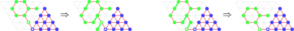
(a) Amoebot $u\in C$ is adjacent to the same amoebot $v\in M$ before and after the translation.

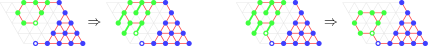
(b) No amoebot in $C$ is adjacent to the same amoebot in $M$ before and after the translation.

Figure 16: Simulation of the nubot model. Let $d$ denote the northeastern direction, $d^{\prime}$ the southwestern direction, and $d^{\prime\prime}$ the northwestern direction. The blue amoebots indicate set $M$. The green amoebots indicate set $C$. The amoebots marked by a white dot indicate amoebots $u$ and $v$.

Woods et al. [60] showed that in the nubot model, the robots are able to self-assemble arbitrary shapes/patterns in an amount of time equal to the worst-case running time for a Turing machine to compute a pixel in the shape/pattern plus an additional factor which is polylogarithmic in its size. While we are able to perform the translations, we do not have the means to let amoebots appear and disappear in the amoebot model. This prevents us from simulating the shape formation algorithm by Woods et al. [60].

4.2 Shape Formation Algorithms for Meta-Modules

Naturally, our meta-modules allow us to simulate shape formation algorithms for lattice-type MRSs of similar shape if we can implement the same movement primitives. This leads us to the following results.

Theorem 4.3.

There is a centralized shape formation algorithm for $m$ rhombical meta-modules that requires $O(\log m)$ rounds and performs $\Theta(m\log m)$ moves overall.

Proof 4.4.

Aloupis et al. [6] proposed a shape formation algorithm for crystalline atoms. It requires $O(\log m)$ rounds and performs $\Theta(m\log m)$ moves overall. The idea is to transform the initial shape to a canonical shape using a divide and conquer approach. The target shape is reached by reversing that procedure. We refer to [6] for the details. The algorithm utilizes the contraction, slide and tunnel primitives which our rhombical meta-modules are capable of (see Section 3.1). Hence, they can simulate this shape formation algorithm.

Theorem 4.5.

There is a centralized shape formation algorithm for $m$ hexagonal meta-modules that requires $O(m)$ rounds. Each module has to perform at most $O(m)$ moves.

Proof 4.6.

Hurtado et al. [27] proposed a shape formation algorithm for hexagonal robots. It requires $O(m)$ rounds and each module has to perform at most $O(m)$ moves. The idea is to compute a spanning tree and to move the robots along the boundary of the tree to a leader module where the robots form a canonical shape, e.g., a line. The target shape is reached by reversing that procedure. We refer to [27] for the details. The algorithm utilizes the rotation primitive which our hexagonal meta-modules are capable of (see Section 3.2). Hence, they can simulate this shape formation algorithm.

5 Locomotion

In this section, we consider amoebot structures capable of locomotion along an even surface. There are three basic types of terrestrial locomotion: rolling, crawling, and walking [26, 33]. We can find biological and artificial examples for each of those. In the following subsections, we will present an amoebot structure for each type and analyze their velocity. In the last subsection, we discuss the transportation of objects.

5.1 Rolling

Animals and robots that move by rolling either rotate their whole body or parts of it. Rolling is rather rare in nature. Among others, spiders, caterpillars, and shrimps are known to utilize rolling as a secondary form of locomotion during danger [8]. Bacterial flagella are an example for a creature that rotates a part of its body around an axle [39].

In contrast, rolling is commonly used in robotic systems mainly in the form of wheels. An example of a robot system rolling as a whole are chain-type MRSs that can roll by forming a loop, e.g., Polypod [61], Polybot [62, 63], CKBot [41, 51], M-TRAN [66, 38], and SMORES [29, 30]. Further, examples for rolling robots can be found in [8, 9].

Our rolling amoebot structure imitates a continuous track that rotates around a set of wheels. Continuous tracks are deployed in various fields, e.g., construction, agriculture, and military. We build our continuous track structure from hexagonal meta-modules of alternating side lengths $\ell$ and $\ell-1$ (see Figure 17). The structure consists of two parts: a connected substrate structure (green meta-modules), and a closed chain of meta-modules rotating along the outer boundary of the substrate (blue meta-modules).

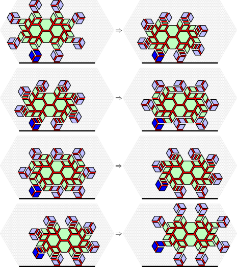
Figure 17: Continuous track structure. The blue meta-modules rotate clockwise around the green meta-modules. We highlight one of the rotating meta-modules in a darker blue.

The continuous track structure moves as follows. The rotating meta-modules that are in contact with the surface release all such bonds with the surface if they rotate away from the surface (see the dark blue meta-module in the third round). Otherwise, they keep these bonds such that the substrate structure is pushed forwards. Note that we have to apply the switching primitive between the rotations. We obtain the initial structure after two rotations. In doing so, the structure has moved a distance of $2\cdot\ell$. By performing the movements periodically, we obtain the following theorem.

Theorem 5.1.

Our continuous track structure composed of hexagonal meta-modules of alternating side lengths $\ell$ and $\ell-1$ moves a distance of $2\cdot\ell$ within each period of constant length.

Butler et al. [10] have proposed another rolling structure for the sliding-cube model that we are able to simulate. The structure resembles a swarm of caterpillars where caterpillars climb over each other from the back to the front [20]. However, due to stalling times, this structure is slower than our continuous track structure. We refer to [10] for the details.

5.2 Crawling

Crawling locomotion is used by limbless animals. According to [31], crawling can be classified into three types: worm-like locomotion, caterpillar-like locomotion, and snake-like locomotion. We will explain the earthworm-like locomotion below and refer to [31] for the other two types. Due to the advantage of crawling in narrow spaces, various crawling structures have been developed for MRSs, e.g., crystalline atoms [36, 48, 49], catoms [11, 13], polypod [61], polybot [63, 67], M-TRAN [38, 66], and origami robots [32].

Our crawling amoebot structure imitates earthworms. An earthworm is divided into a series of segments. It can individually contract and expand each of its segments. Earthworms move by peristaltic crawling, i.e., they propagate alternating waves of contractions and expansions of their segments from the anterior to the posterior part. The friction between the contracted segments and the surface gives the worm grip. This anchors the worm as other segments expand or contract. The waves of contractions pull the posterior parts to the front, and the waves of expansions push the anterior parts to the front. [31, 44]

The simplest amoebot structure that imitates an earthworm is a simple line of $n$ expanded amoebots along the surface (see Figure 18(a)). Each amoebot can be seen as a segment of the worm. Instead of propagating waves of contractions and expansions, we contract and expand the whole structure at once. During each contraction (expansion), we release all bonds between the amoebot structure and the surface except for the ones at the head (tail) of the structure that serve as an anchor. As a result, the contraction (expansion) pulls (pushes) the structure to the front. The simple line has moved by a distance of $n$ along the surface after performing a contraction and an expansion. This is the fastest way possible to move along a surface since we accumulate the movements of all amoebots into the same direction. By performing the movements periodically, we obtain the following theorem.

Theorem 5.2.

A simple line of $n$ expanded amoebots moves a distance of $n$ every $2$ rounds.

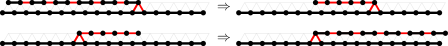
(a) Simple line of amoebots.

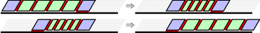
(b) Line of rhombical meta-modules.

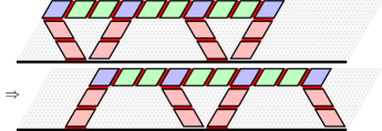
(c) Millipede structure. The red rhombi indicate the legs. The blue and green rhombi indicate the body. The blue rhombi indicate the connectors. Note that the figure only depicts the first half of a period.

Figure 18: Worm and millipede structures.

However, in practice, the contractions and expansions of the whole structure yield high forces acting on the connections within the amoebot structure. We can address this problem by thickening the worm structure. This increases the expansion of the structure and with that its stability. Consider a line of $r$ rhombical meta-modules of side length $\ell-1$ (see Figure 18(b)). Each module can be seen as a segment of the worm structure. Recall that we can contract a rhombical meta-module into a parallelogram (see Figure 8(a)). The line of rhombical meta-modules moves in the same manner as the simple line except for the following two points. First, we utilize the whole meta-module at the front and at the end as an anchor to increase the grip, respectively. Second, only the middle $r-2$ meta-modules participate in the contractions and expansions. The line of rhombical meta-modules moves a distance of $\frac{r-2}{2}\cdot\ell$ along the surface after performing a contraction and an expansion. By performing the movements periodically, we obtain the following theorem.

Theorem 5.3.

A line of $r$ rhombical meta-modules of side length $\ell-1$ moves a distance of $\frac{r-2}{2}\cdot\ell$ every $2$ rounds.

Another problem in practice is friction between the structure and the surface and with that the wear of the structure. The worm structure is therefore poorly scalable in its length such that other types for locomotion are more suitable for large amounts of amoebots.

Most of the cited MRSs at the beginning of this section are very similar to our construction. The construction for crystalline robots is the closest one. Each of these consists of a line of (meta-)modules that are able to contract. Katoy et al. [36] also propose a ‘walking’ structure (see Figure 19). However, the locomotion is still caused by the contraction of the body instead of motions of the legs. So, it is rather a caterpillar-like crawling than a walking movement.

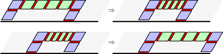
Figure 19: Caterpillar structure. This structure is a replication of the structure by Katoy et al. [36] in the joint movement extension.

5.3 Walking

A wide variety of animals are capable of walking locomotion, e.g., mammals, reptiles, birds, insects, millipedes, and spiders. Just as wide is the variety of differences, e.g., they differ in the number of legs, in the structure of the legs, and in their gait. Walking structures have been built for chain-type MRSs, e.g., M-TRAN [66, 38] and polybot [63, 67].

Our walking amoebot structure imitates millipedes. Millipedes have flexible, segmented bodies with tens to hundreds of legs that provide morphological robustness [52]. They move by propagating leg-density waves from the posterior to the anterior [25, 37]. We build our millipede structure from rhombical meta-modules of side length $\ell-1$ (see Figure 18(c)). Let $p$ denote the number of legs. The body and each leg consists of a line of rhombical meta-modules. All legs have the same size. Let $q$ denote the number of rhombical modules in each leg. We attach each leg to a meta-module of the body and orientate them alternating to the front and to the back. We call those meta-modules connectors. In order to prevent the legs from colliding, we place $q$ meta-modules between two connectors. Altogether, the millipede structure consists of $(2p-1)\cdot q+p$ meta-modules.

In order to move the legs back and forth, we simply apply the realignment primitive (see Figure 8(c)) on all meta-modules within the legs (see Figure 18(c)). We achieve forward motion by releasing all bonds between the surface and the legs moving forwards. In one step, the body moves a distance of $q\cdot\ell$. Note that the number of legs has no impact on the velocity. By continuously repeating these leg movements, we achiegfve a motion similar to the leg-density waves of millipedes. Note that we reach the initial amoebot structure after two leg movements. Hence, we obtain the following theorem.

Theorem 5.4.

Our millipede structure composed of rhombical meta-modules of side length $\ell-1$ with $p$ legs composed of $q$ rhombical meta-modules moves a distance of $2\cdot q\cdot\ell$ within each period of constant length.

In practice, we can reduce the friction by additionally lifting the legs moving forwards (see Figure 20). For that, it suffices to partially contract all meta-modules of the body except for the connectors connected to a leg moving backwards. After the movement, we lower the lifted legs back to the ground. For that, we reverse the contractions within the body.

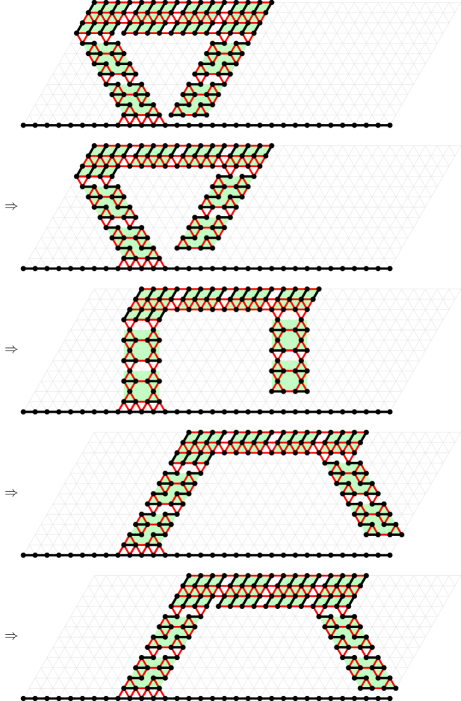
Figure 20: Movement of a millipede. For the sake of simplicity, we only show two legs.

5.4 Transportation

Another important aspect of locomotion is the transportation of objects. The continuous track and worm structure are unsuitable for the transportation of objects due to their unstable top. In the worm structure, we can circumvent that problem by increasing the number of meta-modules not participating in the contractions and expansions. However, this decreases the velocity of the worm structure and increases the friction under the object.

In contrast, the millipede structure provides a rigid transport surface for the transportation of objects (see Figure 21). In practice, a high load introduced by the object on the structure may lead to problems. However, it was shown that millipedes have a large payload-to-weight ratio since they have to withstand high loads while burrowing in leaf litter, dead wood, or soil [25, 52]. The millipede is able to distribute the weight evenly on its legs. Consequently, the millipede structure is well suited for the transportation of objects.

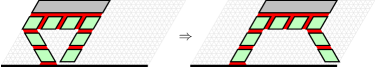
Figure 21: Transportation of objects by the millipede structure. The green rhombi indicate the millipede structure. The gray parallelogram indicates the object.

6 Conclusion and Future Work

In this paper, we have formalized the joint movement extension that were proposed by Feldmann et al. [23]. We have constructed meta-modules of rhombical and hexagonal shape that are able to perform various movement primitives. This allows us to simulate shape formation algorithms of various MRSs. However, our meta-modules are more flexible, e.g., we can move a hexagonal meta-module through two others (see Appendix A). Such new movement primitives may lead to faster shape formation algorithms, e.g., sublinear solutions for hexagonal meta-modules or even arbitrary amoebot structures. Furthermore, we have presented three amoebot structures capable of moving along an even surface. In future work, movement on uneven surfaces can be considered.

Appendix A Moving Meta-Modules through Others

In this section, we show how to move a hexagonal meta-module $H_{1}$ through two other hexagonal meta-modules $H_{2}$ and $H_{3}$ (see Figure 22). We first form six rhombical meta-modules from $H_{1}$ and the amoebots of $H_{2}$ and $H_{3}$ that are located between the old and new position of $H_{1}$. For that, we shift the amoebots along the red lines. Using the realignment primitive and the slide primitive for rhombical meta-modules, we shift the six rhombical meta-modules into the new position of $H_{1}$. Finally, we restore $H_{2}$ and $H_{3}$ by shifting the amoebots along the red lines. Note that we have omitted some necessary reorientations.

Lemma A.1.

We can move a hexagonal meta-module through two other hexagonal meta-modules within $O(1)$ rounds.

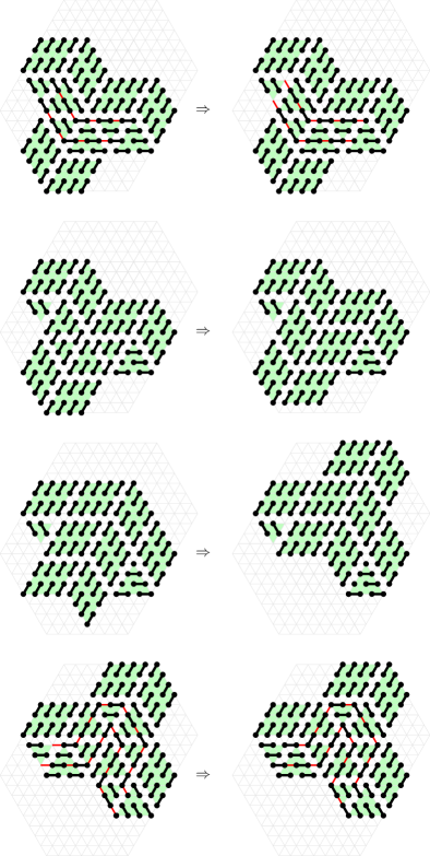
Figure 22: Moving a hexagonal meta-module through two other hexagonal meta-modules. For the sake of clarity, we have omitted the bonds in these figures. In the first and last step, the amoebots move along the red lines.

References

- [1] Hossein Ahmadzadeh, Ellips Masehian, and Masoud Asadpour. Modular robotic systems: Characteristics and applications. J. Intell. Robotic Syst., 81(3-4):317–357, 2016.
- [2] Hugo A. Akitaya, Esther M. Arkin, Mirela Damian, Erik D. Demaine, Vida Dujmovic, Robin Y. Flatland, Matias Korman, Belén Palop, Irene Parada, André van Renssen, and Vera Sacristán. Universal reconfiguration of facet-connected modular robots by pivots: The O(1) musketeers. Algorithmica, 83(5):1316–1351, 2021.
- [3] Abdullah Almethen, Othon Michail, and Igor Potapov. Distributed transformations of hamiltonian shapes based on line moves. Theor. Comput. Sci., 942:142–168, 2023.
- [4] Greg Aloupis, Nadia M. Benbernou, Mirela Damian, Erik D. Demaine, Robin Y. Flatland, John Iacono, and Stefanie Wuhrer. Efficient reconfiguration of lattice-based modular robots. Comput. Geom., 46(8):917–928, 2013.
- [5] Greg Aloupis, Sébastien Collette, Mirela Damian, Erik D. Demaine, Robin Y. Flatland, Stefan Langerman, Joseph O’Rourke, Suneeta Ramaswami, Vera Sacristán Adinolfi, and Stefanie Wuhrer. Linear reconfiguration of cube-style modular robots. Comput. Geom., 42(6-7):652–663, 2009.
- [6] Greg Aloupis, Sébastien Collette, Erik D. Demaine, Stefan Langerman, Vera Sacristán Adinolfi, and Stefanie Wuhrer. Reconfiguration of cube-style modular robots using o(logn) parallel moves. In ISAAC, volume 5369 of Lecture Notes in Computer Science, pages 342–353. Springer, 2008.
- [7] Byoung Kwon An. Em-cube: cube-shaped, self-reconfigurable robots sliding on structure surfaces. In 2008 IEEE International Conference on Robotics and Automation, ICRA 2008, May 19-23, 2008, Pasadena, California, USA, pages 3149–3155. IEEE, 2008. doi:10.1109/ROBOT.2008.4543690.
- [8] Rhodri H Armour and Julian FV Vincent. Rolling in nature and robotics: A review. Journal of Bionic Engineering, 3(4):195–208, 2006.
- [9] Alberto Brunete, Avinash Ranganath, Sergio Segovia, Javier Perez De Frutos, Miguel Hernando, and Ernesto Gambao. Current trends in reconfigurable modular robots design. International Journal of Advanced Robotic Systems, 14(3):1729881417710457, 2017.
- [10] Zack J. Butler, Keith Kotay, Daniela Rus, and Kohji Tomita. Generic decentralized control for lattice-based self-reconfigurable robots. Int. J. Robotics Res., 23(9):919–937, 2004.
- [11] Jason Campbell and Padmanabhan Pillai. Collective actuation. Int. J. Robotics Res., 27(3-4):299–314, 2008.
- [12] Gregory S. Chirikjian. Kinematics of a metamorphic robotic system. In ICRA, pages 449–455. IEEE Computer Society, 1994.
- [13] David Johan Christensen and Jason Campbell. Locomotion of miniature catom chains: Scale effects on gait and velocity. In ICRA, pages 2254–2260. IEEE, 2007.
- [14] Joshua J. Daymude, Kristian Hinnenthal, Andréa W. Richa, and Christian Scheideler. Computing by programmable particles. In Distributed Computing by Mobile Entities, volume 11340 of Lecture Notes in Computer Science, pages 615–681. Springer, 2019.
- [15] Joshua J. Daymude, Andréa W. Richa, and Christian Scheideler. The canonical amoebot model: Algorithms and concurrency control. In DISC, volume 209 of LIPIcs, pages 20:1–20:19. Schloss Dagstuhl - Leibniz-Zentrum für Informatik, 2021.
- [16] Zahra Derakhshandeh, Shlomi Dolev, Robert Gmyr, Andréa W. Richa, Christian Scheideler, and Thim Strothmann. Brief announcement: amoebot - a new model for programmable matter. In SPAA, pages 220–222. ACM, 2014.
- [17] Zahra Derakhshandeh, Robert Gmyr, Andréa W. Richa, Christian Scheideler, and Thim Strothmann. An algorithmic framework for shape formation problems in self-organizing particle systems. In NANOCOM, pages 21:1–21:2. ACM, 2015.
- [18] Zahra Derakhshandeh, Robert Gmyr, Andréa W. Richa, Christian Scheideler, and Thim Strothmann. Universal shape formation for programmable matter. In SPAA, pages 289–299. ACM, 2016.
- [19] Daniel J. Dewey, Michael P. Ashley-Rollman, Michael DeRosa, Seth Copen Goldstein, Todd C. Mowry, Siddhartha S. Srinivasa, Padmanabhan Pillai, and Jason Campbell. Generalizing metamodules to simplify planning in modular robotic systems. In IROS, pages 1338–1345. IEEE, 2008.
- [20] Shlomi Dolev, Sergey Frenkel, Michael Rosenblit, Ram Prasadh Narayanan, and K Muni Venkateswarlu. In-vivo energy harvesting nano robots. In 2016 IEEE International Conference on the Science of Electrical Engineering (ICSEE), pages 1–5, 2016.
- [21] Fabien Dufoulon, Shay Kutten, and William K. Moses Jr. Efficient deterministic leader election for programmable matter. In PODC, pages 103–113. ACM, 2021.
- [22] Adrian Dumitrescu, Ichiro Suzuki, and Masafumi Yamashita. Motion planning for metamorphic systems: feasibility, decidability, and distributed reconfiguration. IEEE Trans. Robotics, 20(3):409–418, 2004.
- [23] Michael Feldmann, Andreas Padalkin, Christian Scheideler, and Shlomi Dolev. Coordinating amoebots via reconfigurable circuits. J. Comput. Biol., 29(4):317–343, 2022.
- [24] Robert Fitch and Zack J. Butler. Million module march: Scalable locomotion for large self-reconfiguring robots. Int. J. Robotics Res., 27(3-4):331–343, 2008.
- [25] Anthony Garcia, Gregory Krummel, and Shashank Priya. Fundamental understanding of millipede morphology and locomotion dynamics. Bioinspiration & Biomimetics, 16(2):026003, dec 2020.
- [26] Shigeo Hirose. Three basic types of locomotion in mobile robots. In Fifth International Conference on Advanced Robotics’ Robots in Unstructured Environments, pages 12–17. IEEE, 1991.
- [27] Ferran Hurtado, Enrique Molina, Suneeta Ramaswami, and Vera Sacristán Adinolfi. Distributed reconfiguration of 2d lattice-based modular robotic systems. Auton. Robots, 38(4):383–413, 2015.
- [28] Norio Inou, Hisato Kobayashi, and Michihiko Koseki. Development of pneumatic cellular robots forming a mechanical structure. In ICARCV, pages 63–68. IEEE, 2002.
- [29] Gangyuan Jing, Tarik Tosun, Mark Yim, and Hadas Kress-Gazit. An end-to-end system for accomplishing tasks with modular robots. In Robotics: Science and Systems, 2016.
- [30] Gangyuan Jing, Tarik Tosun, Mark Yim, and Hadas Kress-Gazit. Accomplishing high-level tasks with modular robots. Auton. Robots, 42(7):1337–1354, 2018.
- [31] Zoltán Juhász and Ambrus Zelei. Analysis of worm-like locomotion. Periodica Polytechnica Mechanical Engineering, 57(2):59–64, 2013.
- [32] Manivannan Sivaperuman Kalairaj, Catherine Jiayi Cai, Pavitra S, and Hongliang Ren. Untethered origami worm robot with diverse multi-leg attachments and responsive motions under magnetic actuation. Robotics, 10(4):118, 2021.
- [33] Matthew Kehoe and Davide Piovesan. Taxonomy of two dimensional bio-inspired locomotion systems. In EMBC, pages 3703–3706. IEEE, 2019.
- [34] Brian T. Kirby, Jason Campbell, Burak Aksak, Padmanabhan Pillai, James F. Hoburg, Todd C. Mowry, and Seth Copen Goldstein. Catoms: Moving robots without moving parts. In AAAI, pages 1730–1731. AAAI Press / The MIT Press, 2005.
- [35] Irina Kostitsyna, Christian Scheideler, and Daniel Warner. Fault-tolerant shape formation in the amoebot model. In DNA, volume 238 of LIPIcs, pages 9:1–9:22. Schloss Dagstuhl - Leibniz-Zentrum für Informatik, 2022.
- [36] Keith Kotay, Daniela Rus, and Marsette Vona. Using modular self-reconfiguring robots for locomotion. In ISER, volume 271 of Lecture Notes in Control and Information Sciences, pages 259–269. Springer, 2000.
- [37] Shigeru Kuroda, Nariya Uchida, and Toshiyuki Nakagaki. Gait switching with phase reversal of locomotory waves in the centipede scolopocryptops rubiginosus. Bioinspiration & Biomimetics, 17(2):026005, mar 2022.
- [38] Haruhisa Kurokawa, Eiichi Yoshida, Kohji Tomita, Akiya Kamimura, Satoshi Murata, and Shigeru Kokaji. Self-reconfigurable M-TRAN structures and walker generation. Robotics Auton. Syst., 54(2):142–149, 2006.
- [39] Michael LaBarbera. Why the wheels won’t go. The American Naturalist, 121(3):395–408, 1983.
- [40] Giuseppe Antonio Di Luna, Paola Flocchini, Nicola Santoro, Giovanni Viglietta, and Yukiko Yamauchi. Shape formation by programmable particles. Distributed Comput., 33(1):69–101, 2020.
- [41] Daniel Mellinger, Vijay Kumar, and Mark Yim. Control of locomotion with shape-changing wheels. In ICRA, pages 1750–1755. IEEE, 2009.
- [42] Satoshi Murata, Haruhisa Kurokawa, and Shigeru Kokaji. Self-assembling machine. In ICRA, pages 441–448. IEEE Computer Society, 1994.
- [43] An Nguyen, Leonidas J Guibas, and Mark Yim. Controlled module density helps reconfiguration planning. In Workshop on the Algorithmic Foundations of Robotics, page TH15–TH27, 2001.
- [44] Hayato Omori, Takeshi Hayakawa, and Taro Nakamura. Locomotion and turning patterns of a peristaltic crawling earthworm robot composed of flexible units. In IROS, pages 1630–1635. IEEE, 2008.
- [45] Andreas Padalkin, Christian Scheideler, and Daniel Warner. The structural power of reconfigurable circuits in the amoebot model. In DNA, volume 238 of LIPIcs, pages 8:1–8:22. Schloss Dagstuhl - Leibniz-Zentrum für Informatik, 2022.
- [46] Irene Parada, Vera Sacristán, and Rodrigo I. Silveira. A new meta-module for efficient reconfiguration of hinged-units modular robots. In ICRA, pages 5197–5202. IEEE, 2016.
- [47] John Romanishin, Kyle Gilpin, and Daniela Rus. M-blocks: Momentum-driven, magnetic modular robots. In IROS, pages 4288–4295. IEEE, 2013.
- [48] Daniela Rus and Marsette Vona. Self-reconfiguration planning with compressible unit modules. In ICRA, pages 2513–2520. IEEE Robotics and Automation Society, 1999.
- [49] Daniela Rus and Marsette Vona. Crystalline robots: Self-reconfiguration with compressible unit modules. Auton. Robots, 10(1):107–124, 2001.
- [50] Hossein Sadjadi, Omid Mohareri, Mohammad Amin Al-Jarrah, and Khaled Assaleh. Design and implementation of hexbot: A modular self-reconfigurable robotic system. J. Frankl. Inst., 349(7):2281–2293, 2012.
- [51] Jimmy Sastra, Sachin Chitta, and Mark Yim. Dynamic rolling for a modular loop robot. Int. J. Robotics Res., 28(6):758–773, 2009.
- [52] Qi Shao, Xuguang Dong, Zhonghan Lin, Chao Tang, Hao Sun, Xin-Jun Liu, and Huichan Zhao. Untethered robotic millipede driven by low-pressure microfluidic actuators for multi-terrain exploration. IEEE Robotics Autom. Lett., 7(4):12142–12149, 2022.
- [53] John W. Suh, Samuel B. Homans, and Mark Yim. Telecubes: Mechanical design of a module for self-reconfigurable robotics. In ICRA, pages 4095–4101. IEEE, 2002.
- [54] Yosuke Suzuki, Norio Inou, Michihiko Koseki, and Hitoshi Kimura. Reconfigurable modular robots adaptively transforming a mechanical structure (numerical expression of transformation criteria of "chobie ii" and motion experiments). In DARS, pages 393–403. Springer, 2008.
- [55] Tommaso Toffoli and Norman Margolus. Programmable matter: Concepts and realization. Int. J. High Speed Comput., 5(2):155–170, 1993.
- [56] Sergei Vassilvitskii, Jeremy Kubica, Eleanor Gilbert Rieffel, John W. Suh, and Mark Yim. On the general reconfiguration problem for expanding cube style modular robots. In ICRA, pages 801–808. IEEE, 2002.
- [57] Sergei Vassilvitskii, Mark Yim, and John W. Suh. A complete, local and parallel reconfiguration algorithm for cube style modular robots. In ICRA, pages 117–122. IEEE, 2002.
- [58] Michael Philetus Weller, Brian T. Kirby, H. Benjamin Brown, Mark D. Gross, and Seth Copen Goldstein. Design of prismatic cube modules for convex corner traversal in 3d. In IROS, pages 1490–1495. IEEE, 2009.
- [59] Paul J. White and Mark Yim. Scalable modular self-reconfigurable robots using external actuation. In IROS, pages 2773–2778. IEEE, 2007.
- [60] Damien Woods, Ho-Lin Chen, Scott Goodfriend, Nadine Dabby, Erik Winfree, and Peng Yin. Active self-assembly of algorithmic shapes and patterns in polylogarithmic time. In ITCS, pages 353–354. ACM, 2013.
- [61] Mark Yim. New locomotion gaits. In ICRA, pages 2508–2514. IEEE Computer Society, 1994.
- [62] Mark Yim, David Duff, and Kimon Roufas. Polybot: A modular reconfigurable robot. In ICRA, pages 514–520. IEEE, 2000.
- [63] Mark Yim, Kimon Roufas, David Duff, Ying Zhang, Craig Eldershaw, and Samuel B. Homans. Modular reconfigurable robots in space applications. Auton. Robots, 14(2-3):225–237, 2003.
- [64] Mark Yim, Paul J. White, Michael Park, and Jimmy Sastra. Modular self-reconfigurable robots. In Encyclopedia of Complexity and Systems Science, pages 5618–5631. Springer, 2009.
- [65] Mark Yim, Ying Zhang, and David Duff. Modular robots. IEEE Spectrum, 39(2):30–34, 2002.
- [66] Eiichi Yoshida, Satoshi Murata, Akiya Kamimura, Kohji Tomita, Haruhisa Kurokawa, and Shigeru Kokaji. Evolutionary synthesis of dynamic motion and reconfiguration process for a modular robot M-TRAN. In CIRA, pages 1004–1010. IEEE, 2003.
- [67] Ying Zhang, Mark Yim, Craig Eldershaw, Dave Duff, and Kimon Roufas. Scalable and reconfigurable configurations and locomotion gaits for chain-type modular reconfigurable robots. In CIRA, pages 893–899. IEEE, 2003.