Feature Expansion for Graph Neural Networks

Abstract

Graph neural networks aim to learn representations for graph-structured data and show impressive performance, particularly in node classification. Recently, many methods have studied the representations of GNNs from the perspective of optimization goals and spectral graph theory. However, the feature space that dominates representation learning has not been systematically studied in graph neural networks. In this paper, we propose to fill this gap by analyzing the feature space of both spatial and spectral models. We decompose graph neural networks into determined feature spaces and trainable weights, providing the convenience of studying the feature space explicitly using matrix space analysis. In particular, we theoretically find that the feature space tends to be linearly correlated due to repeated aggregations. In this case, the feature space is bounded by the poor representation of shared weights or the limited dimensionality of node attributes in existing models, leading to poor performance. Motivated by these findings, we propose 1) feature subspaces flattening and 2) structural principal components to expand the feature space. Extensive experiments verify the effectiveness of our proposed more comprehensive feature space, with comparable inference time to the baseline, and demonstrate its efficient convergence capability.

1 Introduction

Graph Neural Networks (GNNs) have shown great potential in learning representations of graph-structured data, such as social networks, transportation networks, protein interaction networks, etc. (Fan et al., 2019; Wu et al., 2020; Khoshraftar & An, 2022). In this paper, we focus on node representation learning, which is one of the most important tasks in this line of research, where the key is to represent nodes in an informative and structure-aware way.

There are two different types of graph neural networks. One is spatial, which aggregates information from neighboring nodes and updates the representation of the central node. (Velickovic et al., 2018; Xu et al., 2018; Huang et al., 2020a). The spectral type, on the other hand, treats the graph structure matrix, such as the Laplacian matrix, as a transformation for the nodes’ attributes (signals) in the spectral domain (Defferrard et al., 2016; Chien et al., 2021; He et al., 2021, 2022). The aim is to develop flexible functions for the graph structure so that the signals of the nodes can fit the labels appropriately.

Recently, several perspectives for analyzing GNN representations have emerged, such as general optimization functions, denoising frameworks, and spectral graph theory (Zhu et al., 2021; Ma et al., 2021; Balcilar et al., 2021). However, as a determinant of representation learning, feature spaces have not been systematically studied for graph neural networks. In general representation learning, performance depends heavily on the construction of feature spaces with accessible data (Bengio et al., 2013).

In this paper, we propose to fill this gap and investigate the feature space for both spatial and spectral GNNs. Specifically, for theoretical investigations, we first abstract a linear approximation of the GNNs following the studies (Wu et al., 2019a; Xu et al., 2018; Wang & Zhang, 2022). Then, we decompose the GNN components with and without parameters in the linear approximation, where the latter is considered as a feature space built by node attributes and graph structure (e.g., adjacency or Laplacian matrices), and the former denotes the learnable parameters to reweight the features.

Taking advantage of the convenience of decomposition, we examine the feature space of current models. Motivated by that GNNs are expected to fit arbitrary objective, a more comprehensive feature space reflects better representability without any assumption about the data distribution. However, we find theoretically that the feature subspaces of current GNNs are bounded by the weight-sharing mechanism and the limited dimensionality of the node attributes. In order to alleviate the above restrictions and expand the feature space, we proposed 1) feature subspace flattening and 2) structural principal components, respectively. Specifically, the former reweights all feature subspaces independently to obtain a fully expressed representation. The latter adds the principal components of graph structure matrices as a ”complement” to the original feature space. It is emphasized that our proposal makes no assumptions about the graph or the target, which enjoys good generality. We perform extensive experiments on both homophilic and heterophilic datasets to demonstrate the superiority of the proposal.

Our contributions are listed below:

• Starting from representation learning, we provide the first study of the feature space formed in graph-structured data. Based on this view, we study typical spatial and spectral GNNs and identify two problems of existing GNNs caused by bounded feature spaces.

• We then propose two modifications: 1) feature subspace flattening and 2) structural principal components to expand the whole feature space.

• Extensive experiments are performed on homophilic and heterophilic datasets, and our proposal achieves significant improvements, e.g. an average accuracy increase of 32% on heterophilic graphs.

2 Preliminaries

Table 1: Feature space and parameters for GNN models (better viewed in color)

Original formula^∗ Linear approximation formulations GCN $H^{(k+1)}=\sigma\left(\hat{A}H^{(k)}W^{(k)}\right)$ $H^{(K)}={\color[rgb]{1,.5,0}\hat{A}^{K}X}{\color[rgb]{68,115,196}\prod_{i=0}^{K-1}W^{(i)}}$ (Kipf & Welling, 2017) GIN $H^{(k+1)}=\sigma\left((\epsilon^{(k)}I+\hat{A})H^{(k)}W_{0}^{(k)}\right)W_{1}^{(k)}$ $H^{(K)}=\sum_{t=0}^{K}{\color[rgb]{1,.5,0}\hat{A}^{k}X}{\color[rgb]{68,115,196}\sum_{\{q_{0},\cdots,q_{K-t-1}\}\subseteq\{\epsilon^{(0)},\cdots,\epsilon^{(K-1)}\}}\prod_{i}q_{i}\cdot\prod_{j=0}^{K-1}W_{0}^{(j)}W_{1}^{(j)}}$ (Xu et al., 2018) GCNII $H^{(l+1)}=\sigma\left(\left((1-\alpha^{(l)})\hat{A}H^{(l)}+\alpha^{(l)}H^{(0)}\right)\left((1-\beta^{(l)})I+\beta^{(l)}W^{(l)}\right)\right)$ $H^{(K)}=\sum_{l=0}^{K-1}{\color[rgb]{1,.5,0}\hat{A}^{l}X}{\color[rgb]{68,115,196}\prod_{i=L-l}^{L-1}(1-\alpha^{(i)})\alpha^{(L-l-1)}\prod_{j=L-l-1}^{L-1}W^{(j)}\}}+{\color[rgb]{1,.5,0}\hat{A}^{K}}{\color[rgb]{68,115,196}\prod_{h=0}^{K-1}(1-\alpha^{(h)})W^{(h)}}$ (Chen et al., 2020) ARMA $H^{(K)}=\sigma(\tilde{L}H^{(K-1)}W_{1}+XW_{2})$ $H^{(K)}=\sum_{t=0}^{K}{\color[rgb]{1,.5,0}\tilde{L}X}{\color[rgb]{68,115,196}W_{2}^{t}W_{1}^{K-t}}$ (Bianchi et al., 2021) APPNP $H^{(k+1)}=(1-\alpha)\hat{A}H^{(l)}+\alpha H^{(0)};H^{(0)}=\sigma(XW_{1})W_{2}$ $H^{(K)}=\sum_{t=0}^{K}{\color[rgb]{1,.5,0}(1-\alpha)^{t}\hat{A}^{l}H^{(0)}+\sum_{i=0}^{t-1}\alpha(1-\alpha)^{i}\hat{A}^{i}H^{(0)}}{\color[rgb]{68,115,196}W_{1}W_{2}}$ (Klicpera et al., 2019) ChebyNet^∗∗ $H=\sum_{k=0}^{K}P_{k}(\hat{L})XW^{(k)}$ $H^{(K)}=\sum_{t=0}^{K}{\color[rgb]{1,.5,0}P_{t}(\hat{L})X}{\color[rgb]{68,115,196}W^{(t)}}$ (Defferrard et al., 2016) GPRGNN $H=\sum_{k=0}^{K}\gamma^{(k)}\hat{L}^{k}\sigma(XW_{1})W_{2}$ $H^{(K)}=\sum_{t=0}^{K}{\color[rgb]{1,.5,0}\hat{L}^{t}X}{\color[rgb]{68,115,196}\gamma^{(t)}W_{1}W_{2}}$ (Chien et al., 2021) BernNet $H=\sum_{k=0}^{K}\frac{1}{2^{K}}\binom{K}{k}\gamma^{(k)}(2I-\hat{L})^{K-k}\hat{L}^{k}\sigma(XW_{1})W_{2}$ $H^{(K)}=\sum_{t=0}^{K}{\color[rgb]{1,.5,0}\sum_{j=0}^{t}\frac{1}{2^{j}}\tbinom{K}{j}\hat{L}^{t}}{\color[rgb]{68,115,196}\sum_{j=0}^{t}\gamma^{(j)}W_{1}W_{2}}$ (He et al., 2021) ^∗ Without specification, $H^{(0)}=X$. ^∗∗ $T_{k}(x)$ denotes Chebyshev polynomial $P_{0}(x)=1,P_{1}(x)=x,P_{k}(x)=2xP_{k-1}-P_{k-2}$.

In this paper, we focus on the undirected graph $\mathcal{G}=(\mathcal{V},\mathcal{E})$, along with its node attributes of $\mathcal{V}$ as $X\in\mathbb{R}^{n\times d}$ and adjacency matrix $A\in\mathbb{R}^{n\times n}$ to present $\mathcal{E}$. GNNs take the input of the node attributes and the adjacency matrix, and output the hidden node representations, as $H=\mathtt{GNN}(X,A)\in\mathbb{R}^{n\times d}$. By default, we employ the cross-entropy loss function in the node classification task to minimize the difference between node label $Y$ and the obtained representation as $\mathcal{L}(H,Y)=-\sum_{i}Y_{i}\log\mathrm{softmax}(H_{i})$.

Spatial GNNs (with non-parametric aggregation) mostly fall into the message-passing paradigm. For any given node, it essentially aggregates features from its neighbors and updates the aggregated feature,

$$H_{i}^{(k+1)}=\sigma\left(f_{u}\left(H_{i}^{(k)},f_{a}\left({\hat{A}_{ij},H_{j}^{(k)};j\in\mathcal{N}_{i}}\right)\right)\right),$$ (1)

where $\sigma\left(\cdot\right)$ is a non-linear activation function, $H^{(k)}$ indicates the hidden representation in $k$-th layer, $f_{a}$ and $f_{u}$ are the aggregation and updating functions (Balcilar et al., 2021), $\hat{A}=(D+I)^{-1/2}(A+I)(D+I)^{-1/2}$ is the re-normalized adjacency matrix using the degree matrix $D$, and $\mathcal{N}_{i}$ denotes the $1$-hop neighbors.

Here, we provide two examples to specify this general expression. One is the vanilla GCN  (Kipf & Welling, 2017) that adopts the mean-aggregation and the average-update, whose formulation is:

$$H^{(k+1)}=\sigma\left(\hat{A}H^{(k)}W^{(k)}\right).$$ (2)

The second example shows a different update scheme with skip-connection (Xu et al., 2018; Li et al., 2019; Chen et al., 2020), which is defined as follows,

$$H^{(k+1)}=\sigma\left(\alpha^{(k)}H^{(0)}W^{(k)}_{0}+\hat{A}H^{(k)}W^{(k)}_{1}\right),$$ (3)

where $\alpha^{(k)}$ controls the weight of each layer’s skip-connection, $W_{0}^{(k)},W_{1}^{(k)}$ are the transformation weights for the initial layer and the previous one, respectively.

Spectral GNNs (polynomial-based) originally employ the Graph Fourier transforms to get filters (Chung & Graham, 1997), such as using the eigendecomposition of the Laplacian matrix: $\hat{L}=I-\hat{A}=U\Lambda U^{T}$. In recent years, methods of this type have focused more on approximating arbitrary global filters using polynomials (Wang & Zhang, 2022; Zhu & Koniusz, 2020; He et al., 2021), which has shown superior performance and is written as

$$H=\sum_{k=0}^{K}\gamma^{(k)}P_{k}(\hat{L})\sigma(XW_{1})W_{2},$$ (4)

where $P_{k}(\cdot)$ donates a polynomial’s $k$-order term; $\gamma^{(k)}$ is the adaptive coefficients and $W_{1},W_{2}$ are learnable parameters.

In this paper, we focus on the typical instances of the two types of graph neural networks, as indicated in the parentheses above. For spatial models, we focus on those with non-parametric aggregation, excluding learnable aggregation such as (Velickovic et al., 2018) in the analytical parts. Considering the spectral type, we focus on polynomial-based models, and other spectral filters are not included in this paper, e.g. (Levie et al., 2018; Thanou et al., 2014). It is worth noting that these cases dominate the state of the art, and we still include other methods in empirical comparisons.

Primary observation. From the review of GNN models, we can conclude that usually, the node attributes $X$ and the graph structure matrices $\hat{L}/\hat{A}$ are computed first and then some parameter matrices are applied to obtain the final node representation. Starting from this observation, in the following, we extract a linearly approximated framework including GNNs that first construct feature spaces and then apply parameters to reweight them to obtain node representations.

3 Analysis

To perform theoretical investigations of the feature space, we abstract a linear approximation of GNNs based on the success of linearisation attempts of Wu et al. (2019a); Xu et al. (2018); Wang & Zhang (2022). Specifically, we provide a general formulation for the linear approximation of arbitrary graph neural networks. $\overline{\mathtt{GNN}}(X,\hat{A})$ as:

$$H=\overline{\mathtt{GNN}}(X,\hat{A})=\sum_{t=0}^{T-1}{\color[rgb]{1,.5,0}\Phi_{t}(X,\hat{A})}{\color[rgb]{68,115,196}\Theta_{t}},$$ (5)

where $\Phi_{t}(X,\hat{A})\in\mathbb{R}^{n\times d_{t}}$ is the non-parametric feature space constructing function that inputs the graph data (e.g., node attributes and graph structure) and outputs a feature subspace, $\Theta\in\mathbb{R}^{d_{t}\times c}$ is the parameter space to reweight the corresponding feature subspace for each class $c$, and $T$ is a hyper-parameter of the number of the feature subspaces that the GNN contains. In general, in this linear approximation, a GNN model forms $T$ feature subspaces, i.e., $\Phi_{t}$, and outputs the addition of all the reweighted subspaces using the respective parameters $\Theta_{t}$. Note that the (total) feature space is the union of the subspaces as $\Phi=\{\Phi_{t}\}_{t=0,1,\cdots,T-1}$. Similarly, we have the (total) parameters $\Theta=\{\Theta_{t}\}_{t=0,1,\cdots,T-1}$. Besides, the number of the subspaces $T$ that a GNN model obtains is not parallel with its layer/order, for which we will provide some examples in the later revisiting subsection.

In the following, we will first identify the feature space $\Phi$ and the parameters $\Theta$ for existing GNNs. Then, from the perspective of the feature space, we analyze the common mode across different model lines. Finally, we investigate and summarize the problems behind this mode.

3.1 Revisiting Existing Models

Spatial GNNs (with non-parametric aggregation).  We first transform the recursive formula of spatial GNNs, e.g., (1), into an explicit formula, by iterating from the initial node attributes that $H^{(0)}=X$ and ignoring the activation function. Following Section 2, we consider two examples of spatial GNNs: the vanilla GCN (Kipf & Welling, 2017) and the one with skip-connections (Xu et al., 2018).

The linear approximated explicit formula of a $K$-layer is:

$$H^{(K)}={\color[rgb]{1,.5,0}\hat{A}^{K}X}{\color[rgb]{68,115,196}\prod_{i=0}^{K-1}W^{(i)}},$$ (6)

which forms single feature space $\Phi_{0}=\hat{A}^{K}X$ and parameters $\Theta_{0}=\prod_{i=0}^{K-1}W^{(i)}$ with $T=1$. It is a perfect example that the number of GNN layers $K$ is not identical to the number of the subspaces $T$ a GNN forms. While (3) furthermore considers skip-connections, whose $K$-layer linear approximated explicit formula is formualted as:

$$H^{(K)} =\sum_{i=0}^{K-1}{\color[rgb]{1,.5,0}\hat{A}^{i}X}{\color[rgb]{68,115,196}\alpha^{(K-1-i)}W_{0}^{(K-1-i)}\prod_{j=K-i}^{K-1}W_{1}^{(j)}}$$ (7)

$$+{\color[rgb]{1,.5,0}\hat{A}^{K}X}{\color[rgb]{68,115,196}\prod_{h=0}^{K-1}W_{1}^{(h)}}.$$

By this decomposition, this GCN with skip-connections consists of $T=K+1$ feature subspaces. It forms each feature subspace as $\Phi_{t}=\hat{A}^{t}X$. For the first $T-1$ subspaces, the according respective parameters is denoted as $\Theta_{t;t<T-1}=\alpha^{(K-1-t)}W_{0}^{(K-1-t)}\prod_{j=K-t}^{T-1}W_{1}^{(t)}$, and for for the last $\Phi_{T}$, the parameter is $\Theta_{T}=\prod_{h=0}^{T-1}W_{1}^{(h)}$. Please refer to Appendix A.1 for the derivation.

Spectral GNNs (polynomial-based). This type is specified by the explicit formula as (4). We remove the activation function, and obtain the linear approximation of a $K$-order spectral GNNs as:

$$H^{(K)}=\sum_{k=0}^{K}{\color[rgb]{1,.5,0}P_{k}(\hat{L})X}{\color[rgb]{68,115,196}\gamma^{(k)}W^{(0)}}.$$ (8)

We put the learnable polynomial coefficient $\gamma^{(k)}$ together with the parameter matrices. We also combine the shared parametric matrices in (4) as $W^{(0)}=W_{1}W_{2}$. In this way, (8) forms $T=K+1$ feature subspaces, each denoted as $\Phi_{t}=P_{t}(\hat{L})X$, and the parameters used to reweight the respective subspaces are $\Theta_{t}=W^{(0)}W^{(1)}$. See Appendix A.2 for further derivations.

In Table 1, we summarize typical instances of spatial and spectral methods, using different colors to distinguish the feature space $\Phi$ (orange) and the parameters $\Theta$ (blue). It shows that the proposed extracted view (5) can support most methods in both spatial and spectral domains.

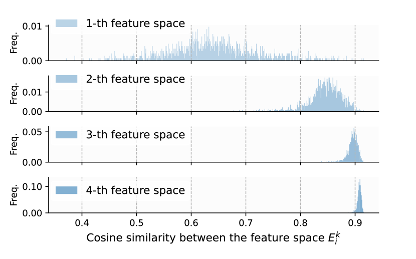
Figure 1: Distribution of the mutual correlation values between the later feature (sub)spaces to the previous total ones.

3.2 Analysis of the Feature Space

In this section, we first give a theoretical argument that the feature subspace of current GNNs obeys asymptotically linear correlation (see Proposition 3.1). Then, we find that the current weight-sharing mechanism weakens the expressiveness of the feature space when the strict linear correlation is satisfied (see Theorem 3.2). In the remainder, we analyze the case where the feature subspaces do not obey strict linear correlation. We find that the feature space is insufficient when the dimensionality of the node attributes is limited and no assumptions can be made about the feature construction (e.g., heterophily).

Table 1 shows that the feature space $\Phi$ in spatial and spectral GNNs is formulated by the multiplication of graph structure matrices function and node attributes, e.g. $\Phi_{k}=P_{k}(\hat{L})X$. We consider $\hat{A}^{k}X$ to be the basic element for each feature subspace since other forms such as $P_{k}(\hat{L})X$ and $\hat{L}$ are all linear transformations of $\hat{A}$. Given this, it can be concluded that the feature subspaces of GNNs are sequentially appended as the spatial layers or the spectral orders of GNNs increase, with the latter subspace being the result of applying the aggregation function to the former.

This monotonous construction of the feature space will lead to a high linear correlation between each feature subspace as presented in Proposition 3.1.

Proposition 3.1.

(its proof can be found in Appendix A.3) Suppose the feature subspaces are constructed sequentially by $\{\Phi_{t}=\hat{A}^{t}X\}_{t}$. As $i\in\mathbb{Z}$ increases, the subspace $\Phi_{t+i}$ gradually tends to be linearly correlated with $\Phi_{t}$.

To better understand the property of Proposition 3.1, we provide a quantitative demonstration using the feature space of GPRGNN (Chien et al., 2021) as an example. We measure the linear correlation of the appended $k$-th feature (sub)space with the previous ones by calculating the mutual correlation values:

$$E^{k}_{i}=\max_{j=0,\cdots,k-1}\mu(\hat{L}^{j}X,\hat{L}^{k}X_{\cdot i}),$$ (9)

where $i$ is the index of the column in $\hat{L}^{k}X$, and $\mu(M_{0},M_{1})=\max_{d_{u}\in M_{0},d_{v}\in M_{1}}\cos(d_{u},d_{v})$ is the mutual-coherence of two matrices, based on the cosine distance $\cos$. In Figure 1, we visualize the distribution of $\{E^{k}_{i}\}$ of all the columns with $k=1,2,3,4$. It confirms that the linear correlation improves significantly with the number of subspaces. Therefore, both theoretical discussions and visualizations show a trend of increasingly linear correlations between feature subspaces with an increasing number of GNN layers/orders.

Since we are dealing with a gradually linear correlation, in the following we identify two questions about the current feature construction when this condition is strictly fulfilled or not, respectively.

Issue 1: Constraint from the weight sharing mechanism. From Table 1 we see that existing GNNs usually share parameter weights between different subspaces. Under the condition of linear correlation, we provide a direct argument that using the weight-sharing method limits the expressiveness of the feature space.

Theorem 3.2.

(its proof can be found in Appendix A.4) Suppose $\Phi_{a},\Phi_{b}\in\mathbb{R}^{n\times d}$ are two linearly correlated feature subspaces, i.e. there exists $W_{a}\in\mathbb{R}^{d\times d}$ such that $\Phi_{a}W_{a}=\Phi_{b}$, and suppose a matrix $B\in\mathbb{R}^{n\times c}$, $c<<d$. If $B$ can be represented by using both subspaces with a common weight $W_{B}$, i.e., $\gamma_{a}\Phi_{a}W_{B}+\gamma_{b}\Phi_{b}W_{B}=B$ and $\gamma_{a},\gamma_{b}\in\mathbb{R}$, then $B$ can always be represented by only one subspace $\Phi_{a}$, i.e., $\Phi_{a}W_{B}^{\prime}=B$ and $W_{B}^{\prime}\in\mathbb{R}^{d\times c}$.

It shows an expressiveness bound of the feature subspaces when they are linearly correlated. While this linearly dependency can be used as redundancy and is widely used in areas such as dictionary learning (Elad, 2010). In particular, an over-determined linear system can be relaxed to an under-determined one when linearly correlated columns are added to the regressor matrix, making it easier to optimize. However, the condition of this benefit is not met in existing GNNs due to the weight-sharing mechanism. In the next section, we propose a modification to break this constraint.

Issue 2: Constraint from limited dimensionality of node attributes. Proposition 3.1 clarifies the tendency of linear correlation between the feature subspaces, but in the first few, this property may not be strictly satisfied. It makes the weight-sharing not so flawed and also weakens the effectiveness of the corresponding modification. In the following, we give a discussion of the condition that the feature spaces are not necessarily linearly correlated, and we consider two limiting scenarios of the dimension $d$ of the node attributes, since the respective discussions are strongly orthogonal.

First, if $d\rightarrow n$, $X$ itself is a sufficient feature space if $X$ is sparse (e.g., bag-of-words features) or each column is linearly independent. Besides, the weight-sharing method sums different feature subspaces by learnable weights $\gamma$ for each. As a result, the optimized sum promotes more of the subspaces that are closer to the labels. Therefore, the core is the assumptions of subspace construction (e.g., homophilic assumptions and hyperparameter search for aggregation functions) and more flexible polynomial functions (e.g., Chebysheb and Bernstein). They all have been widely studied, where the performance of weight-sharing methods is convincing, such as (Wang & Zhang, 2022).

On the other hand, when $d<<n$, the node attributes $X$ have a thin shape, making the regression system strictly over-determined. In addition, without any assumption about the feature space construction, there is hardly an exact solution, even when using linearly correlated copies to perform the expansion (which we will discuss in the next section). Therefore, compared to homophilic graphs, heterophilic graphs are a more severe case, especially since there is hardly any assumption about the feature space construction. For this situation, we propose the other modification below.

4 Proposed Method

Here, we first propose 1) feature subspace flattening for the detrimental condition caused by the weight-sharing mechanism given by Theorem 3.2 and Proposition 3.1. Then, to compensate for the second case when the dimensionality of the node attributes is limited, we propose 2) structural principal components to expand the original feature space.

4.1 Modification 1: Feature Subspaces Flattening

For the first problem, we encourage each feature subspace to be independently expressed of each other in the model and weight them separately. Before giving supporting proof, we provide an illustration of this modification in Figure 2. The benefit of this proposal is given in the following.

Theorem 4.1.

(its proof can be found in Appendix A.5) Suppose $\Phi_{a},\Phi_{b}\in\mathbb{R}^{n\times d}$ are two linearly correlated feature subspaces, i.e., there exits $W_{a}\in\mathbb{R}^{d\times d}$ such that $\Phi_{a}W_{a}=\Phi_{b}$, and a matrix $B\in\mathtt{R}^{d\times c}$, $c<<d$. If $B$ can be expressed by $\Phi_{a}$, i.e., $\Phi_{a}W_{B}=B$, then using both subspaces $\Phi_{a}$ and $\Phi_{b}$ independently, i.e., $\Phi_{a}W_{a}+\Phi_{b}W_{b}=B$, the optimum is more easily achieved than a weight-sharing style.

It follows from this theorem that feature subspace flattening is more effective than weight-sharng methods when the feature subspaces tend to be linearly correlated. For further discussion on parameter matrices that are stacked (e.g., GCN), please refer to Appendix A.7, where the same conclusion is maintained.

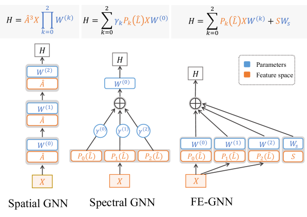
Figure 2: Architecture of our proposal

4.2 Modification 2: Structural Principal Components

Next, we consider the second issue that the dimension of the node attributes is limited. We propose to expand the whole feature space by introducing other feature subspaces.

Table 2: Overall performance of FE-GNN in node classification

Type Baseline Time (ms) Homophilic graphs Heterophilic graphs Cora CiteSeer PubMed Computers Photo Squirrel Chameleon Actor Spatial MLP - 76.70${}_{\pm\text{0.15}}$ 76.67${}_{\pm\text{0.26}}$ 85.11${}_{\pm\text{0.26}}$ 82.62${}_{\pm\text{0.21}}$ 84.16${}_{\pm\text{0.13}}$ 37.86${}_{\pm\text{0.39}}$ 57.83${}_{\pm\text{0.31}}$ 38.99${}_{\pm\text{0.17}}$ GCN 17.42${}_{\pm\text{1.64}}$ 87.69${}_{\pm\text{0.40}}$ 79.31${}_{\pm\text{0.46}}$ 86.71${}_{\pm\text{0.18}}$ 83.24${}_{\pm\text{0.11}}$ 88.61${}_{\pm\text{0.36}}$ 47.21${}_{\pm\text{0.59}}$ 61.85${}_{\pm\text{0.38}}$ 28.61${}_{\pm\text{0.39}}$ GAT 18.06${}_{\pm\text{1.18}}$ 88.07${}_{\pm\text{0.41}}$ 80.80${}_{\pm\text{0.26}}$ 86.69${}_{\pm\text{0.14}}$ 82.86${}_{\pm\text{0.35}}$ 90.84${}_{\pm\text{0.32}}$ 33.40${}_{\pm\text{0.16}}$ 51.82${}_{\pm\text{1.33}}$ 33.48${}_{\pm\text{0.35}}$ GraphSAGE 10.72${}_{\pm\text{0.25}}$ 87.74${}_{\pm\text{0.41}}$ 79.20${}_{\pm\text{0.42}}$ 87.65${}_{\pm\text{0.14}}$ 87.38${}_{\pm\text{0.15}}$ 93.59${}_{\pm\text{0.13}}$ 48.15${}_{\pm\text{0.45}}$ 62.45${}_{\pm\text{0.48}}$ 36.39${}_{\pm\text{0.35}}$ GCNII 8.48${}_{\pm\text{0.24}}$ 87.46${}_{\pm\text{0.31}}$ 80.76${}_{\pm\text{0.30}}$ 88.82${}_{\pm\text{0.08}}$ 84.75${}_{\pm\text{0.22}}$ 93.21${}_{\pm\text{0.25}}$ 43.28${}_{\pm\text{0.35}}$ 61.80${}_{\pm\text{0.44}}$ 38.61${}_{\pm\text{0.26}}$ APPNP 23.74${}_{\pm\text{2.08}}$ 87.92${}_{\pm\text{0.20}}$ 81.42${}_{\pm\text{0.26}}$ 88.16${}_{\pm\text{0.14}}$ 85.88${}_{\pm\text{0.13}}$ 90.40${}_{\pm\text{0.34}}$ 39.63${}_{\pm\text{0.49}}$ 59.01${}_{\pm\text{0.48}}$ 39.90${}_{\pm\text{0.25}}$ Spectral ChebyNet 20.26${}_{\pm\text{1.03}}$ 87.17${}_{\pm\text{0.19}}$ 77.97${}_{\pm\text{0.36}}$ 89.04${}_{\pm\text{0.08}}$ 87.92${}_{\pm\text{0.13}}$ 94.58${}_{\pm\text{0.11}}$ 44.55${}_{\pm\text{0.28}}$ 64.06${}_{\pm\text{0.47}}$ 25.55${}_{\pm\text{1.67}}$ GPRGNN 23.55${}_{\pm\text{1.26}}$ 87.97${}_{\pm\text{0.24}}$ 78.57${}_{\pm\text{0.31}}$ 89.11${}_{\pm\text{0.08}}$ 86.07${}_{\pm\text{0.14}}$ 93.99${}_{\pm\text{0.11}}$ 43.66${}_{\pm\text{0.22}}$ 63.67${}_{\pm\text{0.34}}$ 36.93${}_{\pm\text{0.26}}$ BernNet 36.88${}_{\pm\text{0.84}}$ 87.66${}_{\pm\text{0.26}}$ 79.34${}_{\pm\text{0.32}}$ 89.33${}_{\pm\text{0.07}}$ 88.66${}_{\pm\text{0.08}}$ 94.03${}_{\pm\text{0.08}}$ 44.57${}_{\pm\text{0.33}}$ 63.07${}_{\pm\text{0.43}}$ 36.89${}_{\pm\text{0.30}}$ Unified GNN-LF 52.77${}_{\pm\text{4.50}}$ 88.12${}_{\pm\text{0.06}}$ 83.66${}_{\pm\text{0.06}}$ 87.79${}_{\pm\text{0.05}}$ 87.63${}_{\pm\text{0.05}}$ 93.79${}_{\pm\text{0.06}}$ 39.03${}_{\pm\text{0.08}}$ 59.84${}_{\pm\text{0.09}}$ 41.97${}_{\pm\text{0.06}}$ GNN-HF 53.28${}_{\pm\text{4.51}}$ 88.47${}_{\pm\text{0.09}}$ 83.56${}_{\pm\text{0.10}}$ 87.83${}_{\pm\text{0.10}}$ 86.94${}_{\pm\text{0.06}}$ 93.89${}_{\pm\text{0.10}}$ 39.01${}_{\pm\text{0.51}}$ 63.90${}_{\pm\text{0.11}}$ 42.47${}_{\pm\text{0.07}}$ ADA-UGNN 14.36${}_{\pm\text{0.21}}$ 88.92${}_{\pm\text{0.11}}$ 79.34${}_{\pm\text{0.09}}$ 90.08${}_{\pm\text{0.05}}$ 89.56${}_{\pm\text{0.09}}$ 94.66${}_{\pm\text{0.07}}$ 44.58${}_{\pm\text{0.16}}$ 59.25${}_{\pm\text{0.16}}$ 41.38${}_{\pm\text{0.12}}$ FE-GNN (C) 15.8${}_{\pm\text{0.11}}$ 89.45${}_{\pm\text{0.22}}$ 81.96${}_{\pm\text{0.23}}$ 90.27${}_{\pm\text{0.49}}$ 90.79${}_{\pm\text{0.08}}$ 95.36${}_{\pm\text{0.14}}$ 67.82${}_{\pm\text{0.26}}$ 73.33${}_{\pm\text{0.35}}$ 40.54${}_{\pm\text{0.15}}$ FE-GNN (M) 14.6${}_{\pm\text{0.32}}$ 89.09${}_{\pm\text{0.22}}$ 81.76${}_{\pm\text{0.23}}$ 89.93${}_{\pm\text{0.23}}$ 90.60${}_{\pm\text{0.11}}$ 95.45${}_{\pm\text{0.15}}$ 67.90${}_{\pm\text{0.23}}$ 73.26${}_{\pm\text{0.38}}$ 40.91${}_{\pm\text{0.22}}$

There are two criteria that we consider. One is that the introduced feature subspace should be highly uncorrelated with the existing feature subspace, otherwise, according to the analysis in the previous section, it may not be the same as the previously proposed modification under this condition. The other is that the dimension of the introduced subspace should not be too large, otherwise noise might be included and the computational cost would also increase.

Considering this, for graph-structured data, there are two data matrices, i.e., node attributes and graph structure matrices, and the former has been explicitly exploited as one of the feature subspaces in most GNN models, as summarized in Table 1. On the contrary, structure matrices are used only in combination with node attributes. Given these conditions, we propose to construct the expansion subspace using the truncated SVD of the structural matrix, called structural principal components as modification 2. It naturally provides orthogonal subspaces, and the truncated form limits the dimension of the matrices. Thus, two criteria are met. Specifically, we extract the low-dimensional information for the graph structure to obtain its principal components:

$${S=\tilde{Q}\tilde{V}};\hat{A}=QVR^{T},$$ (10)

where $\tilde{Q},\tilde{V}$ are the principal components and the corresponding singular values. Besides, we prove the effectiveness of this modification in the following theorem.

Theorem 4.2.

(its proof can be found in Appendix A.6) Suppose the dimensionality of the node attributes is much smaller than the number of nodes, i.e., $d<<n,X\in\mathbb{R}^{n\times d}$, and a $z$-truncated SVD of $\hat{L}$, which satisfies $||U_{z}S_{z}-\hat{L}||_{2}<\epsilon$, where $\epsilon$ is a sufficiently small constant. Then the linear system $(\Phi_{k},U_{z}S_{z})W_{B}^{\prime}=B$ can achieve a miner error than the linear system $\Phi_{k}W_{B}=B$.

So far, we have introduced two modifications, and together they contribute to a new proposed GNN model called Feature Expanded Graph Neural Network (FE-GNN). It is shown in Figure 2 and formulated as follows,

$$H=\sum_{k=0}^{K}{\color[rgb]{1,.5,0}P_{k}(\hat{L})X}{\color[rgb]{68,115,196}W^{(k)}}+{\color[rgb]{1,.5,0}S}{\color[rgb]{68,115,196}W_{s}}.$$ (11)

It constructs the feature space in two ways. The first part inherits the polynomial-based GNNs and takes advantage of the multiplication of the polynomials of the structural matrix $P_{k}(\hat{L})$ and the node attributes $X$. Second, we use the principal components of the structural matrices to form another feature subspace $S$. In addition, FE-GNN uses independent parameter matrices $W^{(k)}$ and $W_{s}$ to reweight each feature subspace to provide flexible reweighting.

In particular, the $\Phi_{k}$ and $S$ feature spaces can have unbalanced scales and lead to poor reweighting. Therefore, we add a column-wise normalization to ensure that each column of each feature subspace contributes equally to the whole feature space. Finally, to better verify the importance of the feature space view, our implementation is purely linear without any deep artifices such as activation functions or dropout except for the cross-entropy loss, while we obey the original implementation for the baselines and their non-linearity is preserved.

4.3 Discussion

Our analysis and proposal make few assumptions about the distribution of node attributes, the graph structure, or even their relationships. Since the point view of the feature space is not an analysis method proposed specifically for graph structure data or GNNs, our investigations are more general and jump out of the limitations of other views. For example, graph denoising (Zhu et al., 2021) and spectral graph theory view (Balcilar et al., 2021) both ignore the property of node attributes, which is the key for our second proposal, and instead focus on the transformations of the structure matrices. We provide a more comprehensive comparison of related work in section 5.

In our proposed method, the first modification that flattens the feature subspace improves the effectiveness of each feature subspace, but the number of parameters must be higher because no parameter matrices are shared. In experiments, we surprisingly found relatively low training time costs compared to baselines. Furthermore, the second modification can be misinterpreted as an arbitrary addition of structural information. With this in mind, we will conduct additional experiments with other information extraction methods. Besides, in our approach, the aggregation process can be abstracted as preprocessing to further speed up the training process. We leave this as future work; in our experiments, aggregations are computed during each training session for a fair comparison.

Finally, it is worth noting that the linear approximation is adopted for the non-linear GNNs for the following reasons: 1) it allows us the convenience of a deeper view of the GNN models, 2) linearization is a quite normal setting in the theoretical analysis in general machine learning and deep learning analysis, since the non-linearity can hardly provide rigorous arguments (Wu et al., 2019b; Maddox et al., 2021), and 3) the proposed model is fully consistent with the analytical view of linearity.

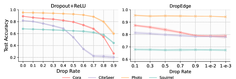
Figure 3: Analysis of the deep artifices on FE-GNN.

5 Other Related Work

Unified perspectives for GNNs. There have been several perspectives for studying GNNs representations. Balcilar et al. (2021) first bridge the spatial methods to the spectral ones, that they assign most of the spatial GNNs with their corresponding graph filters. More specifically, they begin with GNN models’ convolution matrix and then summarize their frequency responses. Ma et al. (2021) regard the aggregation progress of GCN (Kipf & Welling, 2017), GAT (Velickovic et al., 2018), and APPNP (Klicpera et al., 2019) as graph signal denoising problem, which aims to recover a clean signal from an objective and a certain denoising regularization term. Given this, the authors consider generalize the smoothing regularization term to and propose ADA-UGNN. However, it also ignores the property of node attributes but focusing on the flexibility of the denoising functions. Zhu et al. (2021) give a more comprehensive summary of GNNs from an optimization view, which partly overlaps with (Ma et al., 2021)’s opinions of graph signal denoising. They propose GNN-LF/HF with adjustable objective that behaves as a low/high-pass filter.

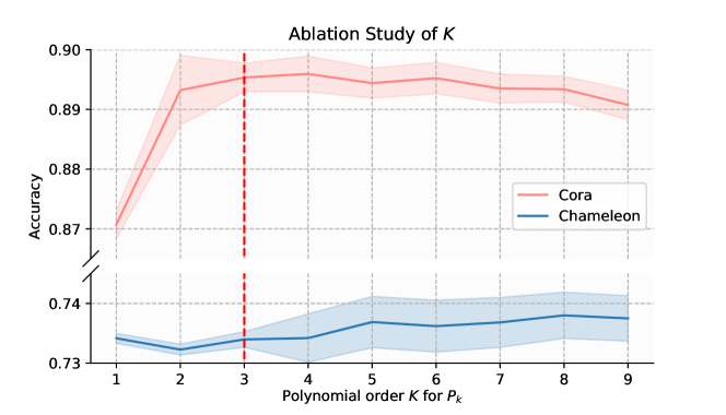
Figure 4: Ablation study of $K$

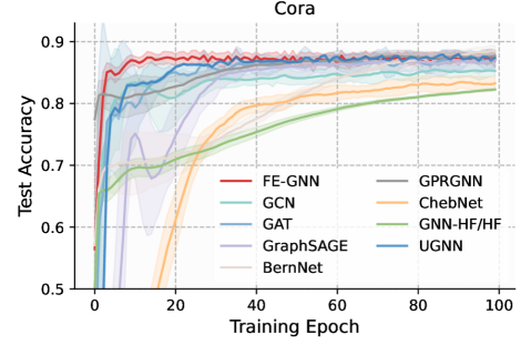
Figure 5: Convergence curve

Trend of flattening feature subspaces. In addition to these unified investigations of GNN representations, another line of related literature is the trend of flattening feature subspaces and the inclusive of graph structure matrices. Initial connection (Li et al., 2019; Chen et al., 2020) is a partial of our first modification that disentangles the dependency between the first two subspaces. There also methods include graph structure information independently, such as LINK (Lim et al., 2021) includes the whole adjacency matrix directly bearing a high parameter consumption. Distance encoding technique encodes the local position using graph structure matrices to supplementary node features (Dwivedi et al., 2020), however, the point view of feature space is untouched. Maurya et al. (2021) also adopt the independent weight for each feature subspace. However, they perform feature selection at the subspace level, while our proposal treats all columns of each subspace equally. Moreover, FE-GNN specifically treats the graph structure as an information source instead of carrying out message-passing. More empirical comparisons are shown in Table 14 in Appendix B.8.

Generally, there have been some scattered attempts to verify the extension perspective of the feature space in the existing work, but due to the lack of a proposal for this view, no more essential conclusions have been drawn.

Over-smoothing. Similar to the linear correlation between each feature subspace (see Proposition 3.1), the strong similarity between node embeddings has been studied extensively, e.g., in the over-smoothing problem (Li et al., 2018; Huang et al., 2020b; Cai & Wang, 2020; Sun et al., 2022). However, our view is from a column-wise perspective (i.e., hidden dimension) and discusses the correlation between the columns of the feature subspaces, while over-smoothing investigations usually focus on the row-wise perspective (i.e., node dimension) and consider the similarity of the output representations of the nodes. They are obviously different, and a further study of these two should also be an interesting future work.

6 Experiments

We evaluate FE-GNN on: (1) node classification results, (2) ablation studies, and (3) efficiency check.

Dataset. We implement our experiments on homophilic datasets, i.e., Cora, CiteSeer, PubMed, Computers, and Photo (Yang et al., 2016; Shchur et al., 2018), and heterophilic Chameleon, Squirrel, and Actor (Rozemberczki et al., 2021; Pei et al., 2020). Among them, Chameleon and Squirrel are two cases that bear problem 2, i.e., limited dimension of node attributes and no homophilic assumptions to use. More details can be found in the appendix B.

Baselines. We compare a list of state-of-the-art GNN methods. For spatial GNNs we have GCN (Kipf & Welling, 2017), GAT (Velickovic et al., 2018), GraphSAGE (Hamilton et al., 2017), GCNII (Chen et al., 2020) and APPNP (Klicpera et al., 2019), where MLP is included as a special case. For spectral methods we take ChebyNet (Defferrard et al., 2016), GPRGNN (Chien et al., 2021) and BernNet (He et al., 2021). We also cover the recent unified models, ADA-UGNN (Ma et al., 2021) and GNN-LF/HF (Zhu et al., 2021). FE-GNN uses the Chebyshev or monomial polynomials to construct the feature space, and we refer to the corresponding versions as FE-GNN (C) and FE-GNN (M), respectively. Please refer to Appendix B.2 for more details on the implementation.

6.1 Node Classification

We test on the node classification task with random 60%/20%/20% splits and summarize the results of 100 runs in Table 2, reporting the average accuracy with a 95% confidence interval. We observe that FE-GNN has almost the best performance on homophilic graphs. In particular, compared to the current SoTA method ADA-UGNN (Ma et al., 2021), which unifies the objectives in both spatial and spectral domains, our FE-GNN achieves a $1.1\%$ accuracy improvement on average on 5 homophilic graph datasets. We attribute the superior performance of GNN-LF/HF on Citeseer to its complex hyperparameter tuning, where more fine-grained constraints of the parameters can be found, which we consider as future work in section 7. Furthermore, FE-GNN achieves on average ${32.0\%}$ improvement on three heterophilic graph datasets than the GCN baseline. It is worth highlighting the huge margin of FE-GNN over others on Chameleon and Squirrel, where they perfectly fit our assumption of the second modification, i.e., heterophilic and limited dimensionality of node attributes. The results of the ablation studies are also consistent with this.

Table 3: Ablation study of 1) flattening feature subspaces

Cora CiteSeer Chameleon Squirrel k=2 $89.15\pm_{0.86}$ $81.97\pm_{1.10}$ $73.41\pm_{1.40}$ $67.37\pm_{0.83}$ k=2 (WS) $87.21\pm_{0.83}$ $78.39\pm_{0.72}$ $72.94\pm_{1.22}$ $66.01\pm_{1.31}$ k=4 $88.56\pm_{2.01}$ $80.19\pm_{0.84}$ $73.27\pm_{1.56}$ $67.40\pm_{0.90}$ k=4 (WS) $87.28\pm_{1.38}$ $77.72\pm_{0.86}$ $73.23\pm_{1.72}$ $66.43\pm_{1.72}$ k=8 $88.92\pm_{0.88}$ $81.11\pm_{0.89}$ $73.85\pm_{1.52}$ $67.93\pm_{2.04}$ k=8 (WS) $86.92\pm_{1.66}$ $77.32\pm_{0.33}$ $73.15\pm_{1.83}$ $66.63\pm_{2.38}$ k=16 $88.26\pm_{0.14}$ $80.54\pm_{1.03}$ $73.88\pm_{1.53}$ $67.82\pm_{1.54}$ k=16 (WS) $87.34\pm_{1.98}$ $78.60\pm_{0.70}$ $72.94\pm_{1.79}$ $66.65\pm_{2.15}$

Table 4: Time consumption of SVD

Cora CiteSeer Chameleon Squirrel Actor Training time (ms) $4000.01\pm 52.23$ $4103.46\pm 133.77$ $2818.21\pm 81.87$ $6096.43\pm 403.95$ $6074.39\pm 547.34$ SVD time (ms) $3.88\pm 0.08$ $8.76\pm 0.05$ $61.80\pm 0.24$ $432.43\pm 0.70$ $3.99\pm 0.02$ # of epochs 252 252 252 271 252 SVD time / Training time (%) 0.097 0.21 2.2 7.1 0.066

Table 5: Ablation study of 2) structural principal components

Cora CiteSeer PubMed Squirrel Chameleon FE-GNN(C) 89.45${}_{\pm\text{0.22}}$ 81.96${}_{\pm\text{0.23}}$ 89.87${}_{\pm\text{0.49}}$ 67.82${}_{\pm\text{0.26}}$ 73.33${}_{\pm\text{0.35}}$ FE-GNN(M) 89.09${}_{\pm\text{0.22}}$ 81.76${}_{\pm\text{0.23}}$ 89.93${}_{\pm\text{0.23}}$ 67.90${}_{\pm\text{0.23}}$ 73.26${}_{\pm\text{0.38}}$ w/o norm 86.23${}_{\pm\text{1.43}}$ 79.32${}_{\pm\text{0.59}}$ 90.27${}_{\pm\text{0.49}}$ 64.70${}_{\pm\text{1.10}}$ 68.25${}_{\pm\text{1.64}}$ w/o $S$ 89.20${}_{\pm\text{0.93}}$ 81.95${}_{\pm\text{0.87}}$ 89.76${}_{\pm\text{0.46}}$ 43.21${}_{\pm\text{0.99}}$ 61.54${}_{\pm\text{1.52}}$ w/o $P_{k}(\hat{L})X_{k>0}$ 71.10${}_{\pm\text{1.72}}$ 74.38${}_{\pm\text{1.01}}$ 86.61${}_{\pm\text{0.54}}$ 67.90${}_{\pm\text{0.96}}$ 73.35${}_{\pm\text{1.21}}$ w/o $P_{k}(\hat{L})X_{k=0}$ 84.70${}_{\pm\text{1.05}}$ 58.60${}_{\pm\text{2.19}}$ 85.84${}_{\pm\text{0.45}}$ 65.75${}_{\pm\text{0.63}}$ 72.61${}_{\pm\text{1.60}}$

6.2 Ablation Studies

We study the contribution of different components and hyperparameter effects in FE-GNN.

Does the feature flattening work? Yes.  In Table 3, we compare our proposal with a weight-sharing (WS) instance where the principal components are retained. It shows that over an increasing number of feature subspaces, the flattening feature subspace is always observed better performance, which verifies the discussion of theorems 3.2 and  4.1.

When do structural principal components work? On limited node attributes and the heterophilic case.  We evaluate FE-GNN on 5 datasets of both homophilic and heterophilic graphs in 3 different feature space constructions: including $w/o\ S$, $w/o\ P_{k}(\hat{L})X_{k=0}$, and $w/o\ P_{k}(\hat{L})X_{k>0}$, which denote the feature space constructions without graph structure, without note attributes, and without the combination of both. In the ablation results of Table 5, we found that $w/o\ S$ works well on homophilic graphs, but fails on heterophilic ones (with limited node attribute dimension), while the other two work inversely. Meanwhile, $w/\ S$ greatly improves the bounded cases, and these results confirm our original intention of proposing structural principal components. In addition, we provide other variants in Appendix B.3 that include structural information as an extension of our discussion in Section 4.3, and row-wise normalization in Appendix A.8, where our proposal is comparably effective.

What proportion of the truncated SVD is appropriate? 94%. We use different ratios of singular vectors and values to construct $S$, i.e., the top $j$ singular values get $r=\sum_{j=1}^{i}V_{jj}/\sum_{j=1}^{n}V_{jj}$ ratio of components. In Figure 6, we show the accuracy of CiteSeer and Chameleon as the ratio of singular values increases, where CiteSeer is robust to variation in the ratio, while Chameleon performs best at $r=94\%$. So we use 94% for further experiments. We provide more SVD results in the Appendix B.6.

At what order is a polynomial sufficient? Around three. We test a progressive order $K$ of polynomials on Cora and Chameleon as shown in Figure 4. The performance in Cora increases from $1$ to $3$ and decreases slightly, while Chameleon shows only small changes. This suggests that order 3 is good enough to achieve near-optimal performance, which is also an advance by flattening the feature subspaces compared to deep GNNs. A more comprehensive comparison can be found in Appendix B.4.

Is linearity sufficient for constructing features? Yes. We apply the nonlinear activation function to FE-GNN and some deep learning training techniques, including Dropout (Agarap, 2018) and DropEdge (Rong et al., 2020), to verify the sufficiency of our linear implementation. In Figure 3, we show the corresponding performance with different drop ratios on four datasets, where both show worse performance when increasing the drop rate. Therefore, our linear construction is sufficient for FE-GNN. These results also argue for more attention to feature space construction to avoid over-application of deep artifices.

6.3 Efficiency Check

Finally, we examine the efficiency of our proposal, including the training time cost and the truncated SVD time. In Table 2, we collect the training time per epoch (ms) for each method, which shows that FE-GNN behaves at a comparable time cost to other baselines, even though it bears more computational cost from the independent feature expression. Note that the time we report includes graph propagation for a fair comparison, although FE-GNN can reduce it further by constructing the feature space in a preprocessing manner. In Figure 5 we compare the convergence time for all methods and observe that FE-GNN consumes the minimum number of training epochs while achieving the highest accuracy, which exactly reveals the conclusion of easier optimization progress from Theorem 4.1. And in table  4, we show the training time and SVD time (as preprocessing), from which we find that the SVD time in the total training time is less than 10%, which confirms the applicability.

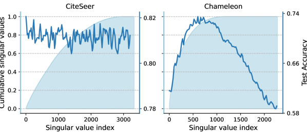
Figure 6: Sensitivity study of truncated SVD

7 Conclusion

In this paper, we provide the feature space view to analyze GNNs, which separates the feature space and the parameters. Together, we provide a theoretical analysis of the existing feature space of GNNs and summarize two issues. We propose 1) feature subspace flattening and 2) structural principal components for these issues. Extensive experimental results verify their superiority.

Limitations Nonlinear cases are not included in our work and will be considered in future work. Also, the correlation between the subspaces should be studied more carefully beyond the linear correlation property; in a sense, the parameters can be further reduced by introducing reasonable constraints. Finally, more feature space construction methods should be discovered for future work.

Appendix A Derivations and Proofs

A.1 Derivation of equation (7)

Iterate (3) from $H^{(0)}=X$, we have

$$H^{(0)} =X$$ (12)

$$H^{(1)} =\alpha^{(0)}XW_{0}^{(0)}+\hat{A}XW_{1}^{(0)}$$ (13)

$$H^{(2)} =\alpha^{(1)}XW_{0}^{(1)}+\hat{A}\alpha^{(0)}XW_{0}^{(0)}W_{1}^{(1)}+\hat{A}^{2}XW_{1}^{(0)}W_{1}^{(1)}$$ (14)

$$H^{(3)} =\alpha^{(2)}XW_{0}^{(2)}+\hat{A}\alpha^{(1)}XW_{0}^{(1)}W_{1}^{(2)}$$ (15)

$$+\hat{A}^{2}\alpha^{(0)}XW_{0}^{(0)}W_{1}^{(1)}W_{1}^{(2)}+\hat{A}^{3}XW_{1}^{(0)}W_{1}^{(1)}W_{1}^{(2)}$$ (16)

$$\cdots$$ (17)

Identify the rule of the iteration, we obtain

$$H^{(k)}=\sum_{i=0}^{l-1}\delta_{i}^{(k)}+\hat{A}^{l}X\prod_{h=0}^{l-1}W_{1}^{(h)},$$ (18)

where $\delta_{i}^{(k)}$ is calculate by:

$$\delta_{i}^{(k)}=\alpha^{(k-1-i)}\hat{A}^{i}XW_{0}^{(k-1-i)}\prod_{j=l-i}^{l-1}W_{1}^{(j)}.$$ (19)

We apply (19) on (18) and put $\alpha^{(k-1-i)}$ back to the learnable parameters $W_{0}^{(k-1-i)}$, and we thus have (7).

A.2 Decomposition of BernNet

BernNet. Different from GPRGNN that utilizes Monomial polynomial, each term of Bernstein polynomial contains another polynomial, such that:

$$P_{k}(\hat{L}) :=\frac{1}{2^{K}}\tbinom{K}{k}(2I-\hat{L})^{K-k}\hat{L}^{k}$$ (20)

$$=\frac{1}{2^{K}}\tbinom{K}{k}\sum_{i=0}^{K-k}2^{i}(-1)^{K-k-i}\tbinom{K-k}{i}\hat{L}^{K-i}$$ (21)

This formulation shows that each element of the BernNet, $P_{k}$, contains a $k$ to $K$-ordered sub-polynomial of $\hat{L}$, where $K$ is the order of a given BernNet. Then we merge the same-ordered element in each $P_{k}$, resulting in feature subspaces $\Phi_{t}$, for which each term contains the components from $P_{0}$ to $P_{t}$.

$$\Phi_{t} =\sum_{j=0}^{t}\frac{1}{2^{K}}\tbinom{K}{j}2^{K-j}\hat{L}^{t}$$ (22)

$$=\sum_{j=0}^{t}\frac{1}{2^{j}}\tbinom{K}{j}\hat{L}^{t}$$ (23)

And the corresponding parameter matrix is $\Theta_{t}=\sum_{j=0}^{t}\gamma^{(j)}W_{1}W_{2}$.

ChebyNet. Its derivation is almost the same as that for BernNet in feature space. Due to the complex structure of the ChebShev polynomials, we omit this calculation and present a substitute to represent each term in Table 1, noted in the footnote. Nevertheless, the rules for the construction of feature spaces hold, namely theorem  3.1, and only different forms of weight distribution are applied to current GNNs in the context of this paper.

A.3 Proofs for Proposition 3.1

First we define the linear correlation of two matrices $M_{1},M_{2}\in\mathbb{R}^{n\times d}$.

Definition A.1.

If there exists a weight matrix $W\in\mathbb{R}^{d\times d}$ such that $||M_{1}W-M_{2}||_{2}\rightarrow 0$, we consider $M_{2}$ to be linearly correlated with $M_{1}$.

Then we consider this to be a linear regression problem, i.e. $M_{1}W=M_{2}$. In this expression, each column of $W$ independently returns each column of $M_{2}$. Without loss of generality, we take an arbitrary column as an example to give the proof.

Suppose $x\in\mathbb{R}^{n\times 1}$ is an arbitrary column of $W$ and $b\in\mathbb{R}^{n\times 1}$ is the corresponding column of $M_{2}$ to recover: $M_{1}x=b$, forming an overdetermined linear system. It has no exact solution for a perfect recovery if no assumption is made about $b$, e.g. $b\in\mathrm{Span}(B)$. However, its minimum error can be minimized if more entries of $b\rightarrow 0$, since it must have the solution of $\mathbf{0}$ for the corresponding part of $x$.

Then we transfer this case to the two subspaces, i.e. $\Phi_{t}=U\Lambda^{t}U^{T}X$ and $\Phi_{i+t}=U\Lambda^{t+i}U^{T}X$, and we consider the linear regression problem:

$$\Phi_{t}W =\Phi_{t+i}$$ (24)

$$U\Lambda^{t}U^{T}XW =U\Lambda^{t+i}U^{T}X$$ (25)

$$U^{T}U\Lambda^{t}U^{T}XW =U^{T}U\Lambda^{t+i}U^{T}X$$ (26)

$$\Lambda^{t}U^{T}XW =\Lambda^{t+i}U^{T}X,$$ (27)

where $\Lambda_{ii}\in[-1,1]$. In the limiting condition, as $i$ increases, more elements of $\Lambda_{t+i}$ approach $0$, then the corresponding part of the regression problem will be: $(\Lambda^{t}U^{T}X)_{\mathcal{C},\cdot}W=0$ as $W\rightarrow 0$ is required as l2-norm regularization for the rest of the linear regression. Then, as $i$ increases, more equation constraints can be relaxed as a regularization, leaving a less overdetermined part of the linear system. Moreover, this can be further relaxed by increasing $t$, because it directly removes more equations from the system. In other words, the linear correlation $W$ is more likely to be obtained. End of proof.

A.4 Proof for Theorem 3.2

This is quite straightforward. It uses some variations of linear algebra.

Given $\gamma_{a}\Phi_{a}W_{B}+\gamma_{b}\Phi_{b}W_{B}=B$, and the linearly correlation $\Phi_{a}W_{a}=\Phi_{b}$, then we have,

$$B =\gamma_{a}\Phi_{a}W_{B}+\gamma_{b}\Phi_{b}W_{B}$$ (28)

$$=(\gamma_{a}\Phi_{a}+\gamma_{b}\Phi_{b})W_{B}$$ (29)

$$=(\gamma_{a}\Phi_{a}+\gamma_{b}\Phi_{a}W_{a})W_{B}$$ (30)

$$=\Phi_{a}(\gamma_{a}I+\gamma_{b}W_{a})W_{B}.$$ (31)

Therefore, $W_{B}^{\prime}=\Phi_{a}(\gamma_{a}I+\gamma_{b}W_{a})W_{B}$. End of the proof.

A.5 Proof for Theorem 4.1

Given $\Phi_{a}W_{B}=B$, and two linearly correlated spaces $\Phi_{a},\Phi_{b}\in\mathbb{R}^{n\times d},\Phi_{a}W_{a}=\Phi_{b}$.

First, in the case of weight sharing, we solve the following linear system with a parameter matrix $W_{B}^{\prime}\in\mathbb{R}^{b\times c}$.

$$\gamma_{a}\Phi_{a}W_{B}^{\prime}+\gamma_{b}\Phi_{b}W_{B}^{\prime} =B$$ (32)

$$\gamma_{a}\Phi_{a}W_{B}^{\prime}+\gamma_{b}\Phi_{a}W_{a}W_{B}^{\prime} =B$$ (33)

$$\Phi_{a}(\gamma_{a}I+\gamma_{b}W_{a})W_{B}^{\prime} =\Phi_{a}W_{B},$$ (34)

Without loss of generality, suppose $B$ is uniquely represented by $\Phi_{a}$ using $W_{B}$, then the solution is $(\gamma_{a}I+\gamma_{b}W_{a})W_{B}^{\prime}=W_{B}$. Remember that $W_{a}$ is given and that it is a nearly determined system.

Second, we consider an independent reweighting method, which is the same as flattening feature subspaces. In this case, we solve the following linear system with two parameter matrices $W_{B}^{a},W_{B}^{b}\in\mathbb{R}^{b\times c}$.

$$\Phi_{a}W_{B}^{a}+\Phi_{b}W_{B}^{b} =B$$ (35)

$$\Phi_{a}W_{B}^{a}+\Phi_{a}W_{a}W_{B}^{b} =B$$ (36)

$$\Phi_{a}(W_{B}^{a}+W_{a}W_{B}^{b}) =\Phi_{a}W_{B}$$ (37)

$$IW_{B}^{a}+W_{a}W_{B}^{b} =W_{B}$$ (38)

This is an underdetermined system, such that $(I,W_{a})({W_{B}^{a}}^{T},{W_{B}^{b}}^{T})^{T}=W_{B}$. Therefore, this independent reweighting is much easier to have an optimal solution compared to weight-sharing methods. End of proof.

A.6 Proof for Theorem 4.2

We provide the proof in two ways. First, we establish a bound on the minima of the linear repression of the SVD of the regressor matrix. Part of the proof A.3:

Assume a linear regression problem $Mx=b$, and $M$ is the regressor matrix with its SVD $M=U_{m}S_{m}V_{m}^{T}$.

$$Mx =b$$ (39)

$$U_{m}S_{m}V_{m}^{T}x =b$$ (40)

$$(U_{m}S_{m}V_{m}^{T})^{-1}U_{m}S_{m}V_{m}^{T}x =(U_{m}S_{m}V_{m}^{T})^{-1}b\leftarrow\mathrm{pseudo-inverse\ using\ \ SVD}$$ (41)

$$\ U_{m}^{T}U_{m}x =V_{m}S_{m}^{-1}U_{m}^{T}b$$ (42)

In equation (41) we inverse the SVD (Silva, 2020) using the invertible property of $U_{m}S_{m}V_{m}^{T}$, $U_{m}^{T}U_{m}=V_{m}V_{m}^{T}=I$. From the equation (42) we can see that the best approximation of $b$ is $\hat{b}=U_{m}U_{m}^{T}b$ if $\hat{x}=V_{m}S_{m}^{-1}U_{m}^{T}b$. Therefore, if $U_{m}U_{m}^{T}\rightarrow I$, then perfect recovery can be further approached.

Then we analyze the change of the regressor matrix between a thin shape feature subspace $\Phi_{k}$ and a concatenation of $(\Phi_{k},U_{z}S_{z})$, where $U_{z},S_{z}$ are the truncated singular vectors and corresponding values of structural matrices, e.g. $\hat{A}$.

• For the case where only $\Phi_{k}$ is used: Since $d<<n$, the singular vectors of $\Phi_{k}$, $U_{k}$ is column-wise full-rank, resulting in its $n$ rows being highly correlated. Given this, $U_{k}U_{k}^{T}$ constructs a rather dense matrix, far from an identity matrix, which leads to a huge gap that uses this feature space as a regressor matrix from a perfect recovery.

• In the concatenation case, when $(\Phi_{k},U_{z}S_{z})$ is used: the singular vector of the concatenation has a permutation difference from the concatenation of their original singular vectors, e.g,

  $$(\Phi_{k},U_{z}S_{z})=(U_{k}S_{k}V_{k}^{T},U_{z}S_{z})=(U_{k},U_{z})\mathrm{DiagCat}(S_{k},S_{z})\mathrm{DiagCat}(V_{k}^{T},V_{z}^{T})=U^{\prime}S^{\prime}V^{\prime T},$$ (43)

  where $\mathrm{DiagCat}()$ is the diagonal concatenation of two square matrices. Since $U^{\prime T}U^{\prime}=I,V^{\prime T}V^{\prime}=I$ and $V^{\prime}V^{\prime T}=I$, this is a reasonable singular vector, but it is a column-wise permutation of $U^{\prime}$ given the order of $S^{\prime}$. Therefore, we represent the singular vectors and values of $(\Phi_{k},U_{z}S_{z})$ as $(U_{k},U_{z})P$ and $P^{T}(S_{k},S_{z})$, where $P\in\mathbb{R}^{(d+z)\times(d+z)}$ is a unitary permutation matrix. Next, we analyze the unitary property of the singular vector $(U_{k},U_{z})P$, i.e., if $(U_{k},U_{z})P((U_{k}^{T},U_{z}^{T})P)^{T}=(U_{k},U_{z})(U_{k}^{T},U_{z}^{T})^{T}\rightarrow I$.

  Since $d<<n$, we ignore the influence of $U_{k}U_{z}^{T}$, $U_{z}U_{k}^{T}$ and $U_{k}U_{k}^{T}$ on the result of $(U_{k},U_{z})(U_{k}^{T},U_{z}^{T})^{T}$, and the $U_{z}$ part dominates the unitary of the singular vectors. Given $||U_{z}S_{z}-\hat{L}||_{2}<\epsilon$, and $\epsilon$ is a small enough constant, a nearly perfect recovery of $\hat{A}$ is achieved by $U_{z}S_{z}$. Then the $U_{z}U_{z}^{T}$ is likely to be identity, given the sparsity property of the structural matrix.

Therefore, the second concatenation of $(\Phi_{k},U_{z}S_{z})$ can achieve a minor error in the regression. End of proof.

Note that we make no assumptions about the distribution of the node attributes or labels.

A.7 More discussion of parameter matrices will be stacked

With a bit of notation abuse, here $W$ is the parameter matrices as $\Theta$ in the equation (5).

Proposition A.2.

GNNs suppress the parameter space of $W$, leading to a partial expression of all columns of the entire feature space and undermining the benefit of adding redundancy to the original one.

Proof.

We summarize the constraints on $W$ in current GNNs as the following: i) in the case of MLP-based implementation (He et al., 2020), all layers share the same $W$, which forces the layer-wise representation parameters into a single matrix; and ii) in the case of layer-wise $W$ (Kipf & Welling, 2017) (Li et al., 2019), each $W_{k+1}$ is built upon its previous one, i.e, $W_{k+1}=\prod_{i=0}^{k+1}W_{i}$. We extract the ideas of these constraints into the following example. Suppose a redundant feature space $U^{\prime}=(d_{0},d_{1},\lambda_{0}d_{0},\lambda_{1}d_{1})$, where $d_{0}\perp d_{1},d_{k}\in\mathbb{R}^{2}$. $x\in\mathrm{Span}\{d_{0},d_{1}\}$ need to be recovered by the elements in $U^{\prime}$.

We deploy the aforementioned two types of constraint on the undecided variables $b_{0},b_{1},b_{2}$, and $b_{3}$: i) $b_{2}=b_{0},b_{3}=b_{1}$, and ii) $b_{2}=\mu b_{0},b_{3}=\mu b_{1}$, where $\mu$ is a trainable scalar. They align with the graph neural networks. We begin by discussing these two cases.

Representing $x$ in the first case, yields:

$$x =b_{0}d_{0}+b_{1}d_{1}+b_{0}\lambda_{0}d_{0}+b_{1}\lambda_{1}b_{1}$$ (44)

$$=(1+\lambda_{0})b_{0}d_{0}+(1+\lambda_{1})b_{1}d_{1}.$$ (45)

Using the unique representation theorem (Hoffman & Kunze, 2004), we have $(1+\lambda_{0})b_{0}=a_{0}$ and $(1+\lambda_{1})b_{1}=a_{1}$. Put it in a matrix multiplication format:

$$\begin{pmatrix}1&0&\lambda_{0}&0\\ 0&1&0&\lambda_{1}\\ \end{pmatrix}\begin{pmatrix}b_{0}\\ b_{1}\\ b_{0}\\ b_{1}\\ \end{pmatrix}=\begin{pmatrix}a_{0}\\ a_{1}\end{pmatrix},$$ (46)

which produces:

$$\begin{pmatrix}1+\lambda_{0}&0\\ 0&1+\lambda_{1}\\ \end{pmatrix}\begin{pmatrix}b_{0}\\ b_{1}\\ \end{pmatrix}=\begin{pmatrix}a_{0}\\ a_{1}\end{pmatrix}.$$ (47)

It holds the closed form that $b_{0}=\frac{a_{0}}{(1+\lambda_{0})},b_{1}=\frac{a_{1}}{(1+\lambda_{1})}$.

Then, we represent $x$ in the second case:

$$x =b_{0}d_{0}+b_{1}d_{1}+\mu b_{0}\lambda_{0}d_{0}+\mu b_{1}\lambda_{1}b_{1}$$ (48)

$$=(1+\mu\lambda_{0})b_{0}d_{0}+(1+\mu\lambda_{1})b_{1}d_{1},$$ (49)

which produces $(1+\mu\lambda_{0})b_{0}=a_{0}$ and $(1+\mu\lambda_{1})b_{1}=a_{1}$. Formulate them in a matrix multiplication:

$$\begin{pmatrix}1&0&\lambda_{0}&0\\ 0&1&0&\lambda_{1}\\ \end{pmatrix}\begin{pmatrix}b_{0}\\ b_{1}\\ \mu b_{0}\\ \mu b_{1}\\ \end{pmatrix}=\begin{pmatrix}a_{0}\\ a_{1}\end{pmatrix}.$$ (50)

This is a under-determined system and gives $b_{0}=\frac{a_{0}}{(1+\mu\lambda_{0})}$, $b_{1}=\frac{a_{1}}{(1+\mu\lambda_{1})}$, $b_{2}=\frac{\mu a_{0}}{(1+\mu\lambda_{0})}$, and $b_{3}=\frac{\mu a_{1}}{(1+\mu\lambda_{1})}$.

We look into the values of $b_{k}$ to get the expressivity of the base $D$. Given the extreme case where $\lambda_{0}\rightarrow 0$, the appended $\lambda_{0}d_{0}$ is constrained while the original one keeps expressing. On the contrary, when $\lambda_{0}\rightarrow\infty$, the original base $d_{0}$ is constrained by $\frac{a_{0}}{(1+\lambda_{0})}$ or $\frac{a_{0}}{(1+\mu\gamma_{0})}$ while the appended one expresses. Besides, for the second case, when $\mu\rightarrow 0$, the corresponding bases are limited by $b_{2},b_{3}\rightarrow 0$. Consequently, both cases lead to partial expression of the the whole feature space.

Finally, compared these two cases, i.e., (60) and (63) to (56), we find that they merely restrict the parameter space of $(b_{0},b_{1},b_{2},b_{3})^{T}$ by either sharing the values of each other or enforcing their linear dependence. Therefore, restricting the parameter space in these two cases leads to partial expression of the the whole feature space. This proof is completed. ∎

A.8 The column-wise normalization in FE-GNN and in current GNNs

Does the column-wise normalization matter? It matters if the node scale is not huge. As shown in Table 5, we find that column-wise normalization works well in most cases, except for PubMed. This may be because the large node scale of PubMed causes the value of the normalized feature space to be tiny.

Then, we include some 10-order polynomial functions to see the different responses of column-wise normalization of these models. Column-wise normalization is defined as forcing $\lVert F_{\cdot i}\rVert_{2}=1$, where we take $F$ as the concatenation of the feature space. We extend this to an arbitrary $k$ times $\lVert F_{\cdot i}\rVert_{2}=1$, i.e., $\lVert F_{\cdot i}\rVert_{2}=k$, which is equivalent to measuring the degree of consistency of each $\lVert F_{\cdot i}\rVert_{2}$. Therefore, we report the standard variance of $\{\lVert F_{\cdot i}\rVert_{2};i=1,2,\cdots\}$, and the smaller the value, the greater the response of the column-wise normalization.

Table 6: The column-wise normalization response for different polyonmials on Cora

	ChebyShev polynomial	Bernstein polynomial	Monomial polynomial
Cora	3.8246	4.7044e-06	0.4947
CiteSeer	34.6432	0.0023	24.4430
Chameleon	660.4274	0.7308	1039.2469
Squirrel	245.6538	0.7063	700.9365

Chebshev, Bernstein, and Monomial polynomials are compared in Table 6. The Bernstein polynomial produces the least variance, indicating that it it promotes the most atomicity compared to other polynomials. This observation is consistent with the narrative in the original BernNet paper (He et al., 2021), where the authors claim that the Bernstein polynomial is more numerically stable than other polynomial functions.

Appendix B Experimental settings

B.1 Dataset details

The datasets are concluded in Table 7, with licenses. Cora, CiteSeer, and PubMed are commonly used homophilic citation networks (Yang et al., 2016). Computers and Photo are homophilic co-bought networks from Amazon (Shchur et al., 2018). For heterophilic datasets, we utilize hyperlinked networks Squirrel and Chameleon from (Pei et al., 2020), and Actor, a subgraph from the film-director-actor network (Rozemberczki et al., 2021). PyG are employed to get these data. Each datasets are split into three parts using random selection: 60% as the training set, 20% as the validation set, and 20% as the test set. We set these datasets to undirected graphs as we assumed in the Preliminaries.

Table 7: Statistics of Datasets

	Cora	CiteSeer	PubMed	Computers	Photo	Squirrel	Chameleon	Actor
$|\mathcal{V}|$	2,708	3,327	19,717	13,752	7,650	5,201	2,277	7,600
$|\mathcal{E}|$	5,278	4,552	44,338	245,861	119,081	217,073	36,101	30,019
# Features	1433	3703	500	767	745	128	128	932
$h(\mathcal{G})$	0.81	0.74	0.80	0.78	0.83	0.22	0.23	0.22
$d(\mathcal{G})$	1.95	1.37	2.25	17.88	15.57	41.74	15.85	3.95

We report the average accuracy (micro F1 score) in the classification task with a 95% confidence interval in all the tables and figures. For each result, we run 100 times on 10 random seeds. We employ Adam for optimization and set the early stopping criteria as a warmup of $50$ pluses patience of $200$ for a maximum of $100$ epochs. We conduct all the experiments on the machine with NVIDIA 3090 GPU (24G) and Intel(R) Xeon(R) Platinum 8260L CPU @ 2.30GHz.

B.2 Searching space for baselines hyper-parameters

For FE-GNN, we turn the following hyper-parameters by the grid search.

• Learning rate: $\{0.01,0.05,0.1\}$

• Weight decay: $\{0.0005,0.001,0.005,0.01,0.02,0.05\}$

• $|S|$ for homophilic graphs: $\{0,10,50,100,200,500,1000,2000\}$

• $|S|$ for heterophilic graphs: $\{500,600,700,800,900,1000,1500,2000\}$

• Suggested $|S|$: the whole hundred from the 94% singular values

• Hidden size: $64$

• Ranks $k$ of the polynomial $P_{k}(\hat{L})$: $\{0,1,2,3\}$

Table 8: The universally used hyper-parameters for FE-GNN.

	lr	weight decay	$|S|$	hidden	$k$
Cora	0.01	0.01	50	64	3
CiteSeer	0.01	0.02	100	64	1
PubMed	0.01	0.005	100	64	3
Computers	0.01	0.0005	1000	64	3
Photo	0.01	0.0005	500	64	3
Squirrel	0.01	0.001	2000	64	3
Chameleon	0.01	0.0005	700	64	3
Actor	0.01	0.001	10	64	0

Table 9: The turned hyper-parameters for the baselines.

lr weight decay dropout hidden layers/ranks others MLP {0.01, 0.05} 0.0005 {0.5, 0.6, 0.8} 64 2 - GCN {0.01, 0.05} 0.0005 {0.5, 0.6, 0.8} 64 {2,3} - GAT {0.01, 0.05} 0.0005 {0.5, 0.6, 0.8} 64 {2,3} $heads$:{1,8} GraphSAGE {0.01, 0.05} 0.0005 {0.5, 0.6, 0.8} 64 {2,3} - GCNII {0.01, 0.05} 0.0005 0.5 64 {2,4,10} $\alpha,\theta$:{0.1, 0.2, 0.5, 0.8, 0.9} APPNP {0.01, 0.05} 0.0005 0.5 64 {2,3,4,5,8} $\alpha$:{0.1, 0.2, 0.5, 0.8, 0.9} ChebNet {0.005, 0.01, 0.05} {0.0, 0.0005} {0.1, 0.2, 0.5} 64 10 - GPRGNN {0.005, 0.01, 0.05} {0.0, 0.0005} {0.1, 0.2, 0.5} 64 10 - BernNet {0.005, 0.01, 0.05} {0.0, 0.0005} {0.1, 0.2, 0.5} 64 10 $prop\_drate$:{0.001,0.02,0.01,0.05} $prop\_lr$:{0.0, 0.1, 0.2, 0.5, 0.6, 0.7, 0.9} ADA-GNN {0.05, 0.01} {0.0005, 0.00005} {0.2,0.5,0.8} 64 {2,5,10} $s$:{1,9,19,29} GNN-LF 0.01 0.005 0.5 64 10 $\alpha,\mu$: {0.1, 0.2, 0.3, 0.4, 0.5, 0.6, 0.8, 0.9} GNN-HF 0.01 0.005 0.5 64 10 $\alpha,\beta$: {0.1, 0.2, 0.3, 0.4, 0.5, 0.6, 0.8, 0.9}

Table 8 represents the hyper-parameters searched for the baselines used in our experiments. We prioritize their original released code repository, and the ranges of turning parameters are according to their papers.

• MLP, GCN, GAT GraphSAGE, APPNP, GCNII are implemented with PyG. 

• ChebNet is implemented according to the code style of BernNet/GPRGNN.

• GPRGNN is implemented according to its original code repository. 

• BernNet is implemented according to its original code repository. 

• ADA-UGNN is implemented according to its original code repository. 

• GNN-HF/LF are implemented according to its original code repository. 

B.3 Other transformations for compacting graph structure information

We add other possible transformations to extract compacted information from the normalized adjacency matrix $\hat{A}$. We compare them in detail:

• KernelPCA: a non-linear kernel PCA method using the Radial Basis Function (RBF).

• FastICA: a fast version of Independent Component Analysis, which is a linear method.

• IsoMap: a nonlinear dimensionality reduction method based on spectral theory.

• LINKX (Lim et al., 2021): an MLP architecture for graph-structured data that includes the graph adjacency matrix as part of the feature space. Due to its inferior performance compared to other baselines, such as GCNII, we exclude it from our main comparisons in the main context.

All of them can be easily implemented using the $\mathtt{sklearn}$ package. As shown in the table 10, our chosen truncated SVD has comparable performance and we stick with it for further analysis in the main text. We regard further investigation of the complex extraction methods as future work, which is beyond the scope of this paper.

Cora CiteSeer Chameleon Squirrel Photo None $89.20_{\pm 0.93}$ $81.95_{\pm 0.87}$ $61.54_{\pm 1.52}$ $43.21_{\pm 0.99}$ - Truncated-SVD $\textbf{89.45}_{\pm 0.22}$ $81.96_{\pm 0.23}$ $73.33_{\pm 0.35}$ $67.90_{\pm 0.23}$ $\textbf{95.45}_{\pm 0.15}$ KernelPCA $88.61_{\pm 0.82}$ $\textbf{81.99}_{\pm 1.11}$ $\textbf{73.66}_{\pm 1.45}$ $\textbf{68.79}_{\pm 1.13}$ $95.36_{\pm 0.51}$ FastICA $88.77_{\pm 1.09}$ $81.92_{\pm 1.00}$ $73.32_{\pm 1.37}$ $68.12_{\pm 0.97}$ $95.30_{\pm 0.22}$ IsoMap $88.54_{\pm 0.86}$ $82.07_{\pm 1.15}$ $67.00_{\pm 1.54}$ $54.47_{\pm 0.87}$ $94.88_{\pm 0.34}$ LINKX - - $68.42_{\pm 1.38}$ $61.81_{\pm 1.80}$ -

Table 10: Comparing the transformations in compacting the normalized adjacency matrix

B.4 Results of FE-GNN using different polynomial orders

In the main text, we implement the polynomial order $K$ in the range of three based on the empirical observations, e.g. Figure 4. Here we provide more comprehensive results for different choices of $K$.

Table 11 shows that we can find better $K$ in a wider range, although the improvement may be marginal.

$K$ 4 5 6 7 8 9 Cora $89.60\pm 0.30$ $89.44\pm 0.25$ $89.52\pm 0.26$ $89.35\pm 0.24$ $89.34\pm 0.22$ $89.08\pm 0.25$ CiteSeer $80.66\pm 1.09$ $81.15\pm 1.06$ $81.11\pm 0.89$ $80.83\pm 1.07$ $80.54\pm 1.03$ $80.10\pm 1.02$ Computers $91.01\pm 0.46$ $90.90\pm 0.51$ $90.98\pm 0.42$ $90.77\pm 0.39$ $90.82\pm 0.41$ $90.45\pm 0.32$ Chameleon $73.42\pm 0.40$ $73.69\pm 0.43$ $73.62\pm 0.43$ $73.68\pm 0.42$ $73.80\pm 0.39$ $73.75\pm 0.38$ Squirrel $68.26\pm 0.78$ $68.41\pm 0.88$ $68.55\pm 0.82$ $68.83\pm 0.68$ $68.92\pm 0.76$ $69.06\pm 0.93$

Table 11: Comparison of different $K$ within $10$

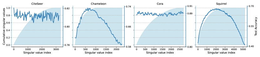
Figure 7: More results of SVD

B.5 Results of FE-GNN on public splits

We additionally add experiments of FE-GNN on the public splits from Geom-GCN (Pei et al., 2020), as shown in the following Table 12. We can see that our proposal still achieves comparable performance. However, the linearity of FE-GNN may constrain its capability in few-shot settings, which is also observed in SGC (Wu et al., 2019b).

Table 12: Comparisons of FE-GNN on public splits

	Cora	CiteSeer	PubMed
FE-GNN (Ours)	$89.13\pm 1.30$	$79.13\pm 1.54$	$89.88\pm 0.64$
GCNII	$88.37\pm 1.25$	$77.33\pm 1.48$	$90.15\pm 0.43$

B.6 More about SVD

In the main test, we append the results to CiteSeer and Squirrel to better verify the importance of the principal components in extracting information from the adjacency matrix in $S_{j}$. As shown in Figure 7 below, we find the exact results we shared in section 6. Cora and CiteSeer both 1) have a smoothing distribution of the singular values and 2) the information from the graph structure is less important than the node features and their interaction, therefore the change in performance is more stable with the introduction of more principal components. On the other hand, Chameleon and Squirrel 1) have a more centralized distribution of singular values and 2) graph structure is more important information, resulting in a tendency of performance to first increase and then decrease. In general, we can achieve satisfactory results on both types of data sets when 94% of the principal components are included.

Here, we offer more intuition about the use of principal components. The principal components project and summarize larger correlated variables into smaller and more interpretable axes of variation. It is ideal for $S_{j}$ to embody the graph structure information from the adjacency matrix because the adjacency matrix is sparse and high-dimensional, but each node is topologically correlated. However, the different components must be distinct from each other to be interpretable, otherwise, they just represent random directions, which leads to noise.

B.7 Comparisons of structural principal components to a random/trainable bias term

To further evaluate the contribution of the proposed SVD space - we would like to emphasize that the SVD space encodes the structure information of the adjacency matrix, which should also be a critical character of GNNs’ feature space. To verify that this structure information is indispensable and cannot be replaced by a structure-free matrix, we provide the following two experiments, both of which perform the replacement on the SVD part $SW_{s}$, where $S$ is the fixed structural principal components matrix and $W_{s}$ is the corresponding learnable weight matrix.

The first experiment, labeled ’$CW_{c}$ (random/orthogonal)’, replaces the structural components $S$ as a random matrix $C$ with the corresponding weights $W_{c}$ to be learned. The other setting, denoted ’$C$ (random/orthogonal)’, replaces the sum $SW_{s}$ as a randomly initialized bias term $C$ to be learned. For a fair comparison with the orthogonal SVD $S$, we add orthogonal initialization variants to both experiments, denoted ’(orthogonal)’. And the ’(random)’ suffix represents the ’xavier_normal’ initialization. The results are shown in Table 13; it shows both $C$ and $CW_{c}$ perform worse than our proposal, especially on the heterophilic Chameleon and Squirrel datasets, which justifies our discussion of the structural principal components.

Table 13: Comparisons of structural principal components and learnable bias

	Cora	CiteSeer	Chameleon	Squirrel	Computers	Photo
FE-GNN (ours)	$89.45\pm 0.22$	$81.96\pm 0.23$	$73.33\pm 0.35$	$67.90\pm 0.23$	$90.79\pm 0.08$	$95.45\pm 0.15$
FE-GNN w/o $S$	$89.20\pm 0.93$	$81.95\pm 0.87$	$61.54\pm 1.52$	$43.21\pm 0.99$	$88.48\pm 0.80$	$94.94\pm 0.79$
$CW_{c}$ (random)	$89.07\pm 1.17$	$81.54\pm 1.38$	$54.93\pm 1.89$	$43.13\pm 1.37$	$89.54\pm 0.83$	$94.56\pm 1.05$
$CW_{c}$ (orthogonal)	$89.31\pm 1.20$	$81.65\pm 1.34$	$55.96\pm 2.00$	$36.87\pm 1.09$	$88.62\pm 0.64$	$94.87\pm 0.73$
$C$ (random)	$89.03\pm 1.34$	$80.83\pm 1.20$	$61.03\pm 2.18$	$43.32\pm 1.25$	$88.85\pm 0.89$	$93.46\pm 3.55$
$C$ (orthogonal)	$89.16\pm 1.28$	$80.99\pm 1.24$	$61.17\pm 2.09$	$43.09\pm 1.34$	$88.94\pm 0.78$	$94.84\pm 0.79$

B.8 More results of FSGNN (Maurya et al., 2021)

We append some experimental results of FSGNN; we adopt the grid search on the range that their original paper reported (Table 5 of (Maurya et al., 2021)), and the results are shown in Table 14. We could see that it cannot achieve better performance on both homophilic and heterophilic datasets.

Table 14: Comparisons of FSGNN on random 60/20/20 splits

	Cora	CiteSeer	PubMed	Chameleon	Squirrel
FE-GNN (Ours)	$89.45\pm 0.22$	$81.96\pm 0.23$	$90.79\pm 0.08$	$73.33\pm 0.35$	$67.90\pm 0.23$
FSGNN	$87.01\pm 1.61$	$79.45\pm 1.78$	$90.71\pm 0.68$	$66.33\pm 1.04$	$54.62\pm 1.57$

Appendix C Additional Feature Space Perspective Explanations

We give a simple illustration from the point of view of using graph structure data, where node attributes and graph structure are the only sources of information. We can think of a pie chart, as shown in Figure 8, where the proportions in blue, yellow, and green colors represent node attributes (e.g., $X$), graph structure (e.g., $S$), and their combination (e.g., $LX$)’s contribution to the overall expressiveness of the feature space. Under different conditions of the graph, each part has different proportions. For example, if the graph is more homophilic, then the combination of the part (in green) contributes more. And if the dimensionality of node attributes is limited, then the proportion of node attributes (in blue) is compact. In general, the task of graph representation learning is to take full advantage of all these three pieces of information. Therefore, from a feature space view, it naturally treats each piece of information equally and aims to construct an extensive feature space that includes all three pieces in the pie chart. In addition, it shows that FE-GNN should be less effective when $d\rightarrow n$, because the feature space is essentially adequate.

However, traditional GNN models consider the graph structure as an information path to do message-massing, i.e., propose to aggregate more hops from neighbors. Since they are restricted to avoid that the graph structure is actually another information source, they could only include two parts in the piechart where the individual graph structure (in yellow) is missing. Therefore, if the node attributes are limited and the graph obeys heterophily, only the feature space view can do a good job by including the graph structure as an individual information source.

Furthermore, the difference in feature space between the homophilic and heterophilic graphs could be: the combination part (in green) of the homophilic pie chart is much larger than that of the heterophilic one. This difference is particularly strong when we look at another part of the feature subspace - the node attributes. The proportion of node attributes $X\in\mathbb{R}^{n\times d}$ (in blue) of the pie chart depends on the dimensionality $d$. If $d\rightarrow n$, (we reasonably assume that the high-dimensional node attributes are sparse here), then the node attributes themselves could form an extensive feature space, making the proportion large and the individual graph structure less important. However, if both the graph obeys heterophily and the node attributes are limited, then the remaining feature subspace of the graph structure (in yellow) is so important; this is also consistent with our ablation study in Table 5, especially for Chameleon and Squirrel.

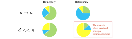
Figure 8: Example diagram of feature space

References

- Agarap (2018) Agarap, A. F. Deep learning using rectified linear units (relu). arXiv preprint arXiv:1803.08375, 2018.
- Balcilar et al. (2021) Balcilar, M., Renton, G., Héroux, P., Gaüzère, B., Adam, S., and Honeine, P. Analyzing the expressive power of graph neural networks in a spectral perspective. In 9th International Conference on Learning Representations, ICLR 2021, Virtual Event, Austria, May 3-7, 2021, 2021.
- Bengio et al. (2013) Bengio, Y., Courville, A., and Vincent, P. Representation learning: A review and new perspectives. IEEE transactions on pattern analysis and machine intelligence, 35(8):1798–1828, 2013.
- Bianchi et al. (2021) Bianchi, F. M., Grattarola, D., Livi, L., and Alippi, C. Graph neural networks with convolutional arma filters. IEEE Transactions on Pattern Analysis and Machine Intelligence, 2021.
- Cai & Wang (2020) Cai, C. and Wang, Y. A note on over-smoothing for graph neural networks. arXiv preprint arXiv:2006.13318, 2020.
- Chen et al. (2020) Chen, M., Wei, Z., Huang, Z., Ding, B., and Li, Y. Simple and deep graph convolutional networks. In International Conference on Machine Learning, pp. 1725–1735. PMLR, 2020.
- Chien et al. (2021) Chien, E., Peng, J., Li, P., and Milenkovic, O. Adaptive universal generalized pagerank graph neural network. In 9th International Conference on Learning Representations, ICLR 2021, Virtual Event, Austria, May 3-7, 2021, 2021.
- Chung & Graham (1997) Chung, F. R. and Graham, F. C. Spectral graph theory. American Mathematical Soc., 1997.
- Defferrard et al. (2016) Defferrard, M., Bresson, X., and Vandergheynst, P. Convolutional neural networks on graphs with fast localized spectral filtering. Advances in neural information processing systems, 29, 2016.
- Dwivedi et al. (2020) Dwivedi, V. P., Joshi, C. K., Laurent, T., Bengio, Y., and Bresson, X. Benchmarking graph neural networks. arXiv preprint arXiv:2003.00982, 2020.
- Elad (2010) Elad, M. Sparse and redundant representations: from theory to applications in signal and image processing, volume 2. Springer, 2010.
- Fan et al. (2019) Fan, W., Ma, Y., Li, Q., He, Y., Zhao, E., Tang, J., and Yin, D. Graph neural networks for social recommendation. In The world wide web conference, pp. 417–426, 2019.
- Hamilton et al. (2017) Hamilton, W., Ying, Z., and Leskovec, J. Inductive representation learning on large graphs. Advances in neural information processing systems, 30, 2017.
- He et al. (2021) He, M., Wei, Z., Xu, H., et al. Bernnet: Learning arbitrary graph spectral filters via bernstein approximation. Advances in Neural Information Processing Systems, 34, 2021.
- He et al. (2022) He, M., Wei, Z., and Wen, J.-R. Convolutional neural networks on graphs with chebyshev approximation, revisited. arXiv preprint arXiv:2202.03580, 2022.
- He et al. (2020) He, X., Deng, K., Wang, X., Li, Y., Zhang, Y., and Wang, M. Lightgcn: Simplifying and powering graph convolution network for recommendation. In Proceedings of the 43rd International ACM SIGIR conference on research and development in Information Retrieval, pp. 639–648, 2020.
- Hoffman & Kunze (2004) Hoffman, K. and Kunze, R. A. Linear Algebra. PHI Learning, second edition, 2004. ISBN 8120302702.
- Huang et al. (2020a) Huang, Q., He, H., Singh, A., Lim, S.-N., and Benson, A. R. Combining label propagation and simple models out-performs graph neural networks. arXiv preprint arXiv:2010.13993, 2020a.
- Huang et al. (2020b) Huang, W., Rong, Y., Xu, T., Sun, F., and Huang, J. Tackling over-smoothing for general graph convolutional networks. arXiv preprint arXiv:2008.09864, 2020b.
- Khoshraftar & An (2022) Khoshraftar, S. and An, A. A survey on graph representation learning methods. arXiv preprint arXiv:2204.01855, 2022.
- Kipf & Welling (2017) Kipf, T. N. and Welling, M. Semi-supervised classification with graph convolutional networks. In 5th International Conference on Learning Representations, ICLR 2017, Toulon, France, April 24-26, 2017, Conference Track Proceedings, 2017.
- Klicpera et al. (2019) Klicpera, J., Bojchevski, A., and Günnemann, S. Predict then propagate: Graph neural networks meet personalized pagerank. In 7th International Conference on Learning Representations, ICLR 2019, New Orleans, LA, USA, May 6-9, 2019, 2019.
- Levie et al. (2018) Levie, R., Monti, F., Bresson, X., and Bronstein, M. M. Cayleynets: Graph convolutional neural networks with complex rational spectral filters. IEEE Transactions on Signal Processing, 67(1):97–109, 2018.
- Li et al. (2019) Li, G., Muller, M., Thabet, A., and Ghanem, B. Deepgcns: Can gcns go as deep as cnns? In Proceedings of the IEEE/CVF international conference on computer vision, pp. 9267–9276, 2019.
- Li et al. (2018) Li, Q., Han, Z., and Wu, X. Deeper insights into graph convolutional networks for semi-supervised learning. In Proceedings of the Thirty-Second AAAI Conference on Artificial Intelligence, pp. 3538–3545. AAAI Press, 2018.
- Lim et al. (2021) Lim, D., Hohne, F., Li, X., Huang, S. L., Gupta, V., Bhalerao, O., and Lim, S. N. Large scale learning on non-homophilous graphs: New benchmarks and strong simple methods. Advances in Neural Information Processing Systems, 34:20887–20902, 2021.
- Ma et al. (2021) Ma, Y., Liu, X., Zhao, T., Liu, Y., Tang, J., and Shah, N. A unified view on graph neural networks as graph signal denoising. In Proceedings of the 30th ACM International Conference on Information & Knowledge Management, pp. 1202–1211, 2021.
- Maddox et al. (2021) Maddox, W. J., Tang, S., Moreno, P. G., Wilson, A. G., and Damianou, A. C. Fast adaptation with linearized neural networks. In The 24th International Conference on Artificial Intelligence and Statistics, AISTATS, volume 130, pp. 2737–2745. PMLR, 2021.
- Maurya et al. (2021) Maurya, S. K., Liu, X., and Murata, T. Simplifying approach to node classification in graph neural networks. arXiv preprint arXiv:2111.06748, 2021.
- Pei et al. (2020) Pei, H., Wei, B., Chang, K. C.-C., Lei, Y., and Yang, B. Geom-gcn: Geometric graph convolutional networks. arXiv preprint arXiv:2002.05287, 2020.
- Rong et al. (2020) Rong, Y., Huang, W., Xu, T., and Huang, J. Dropedge: Towards deep graph convolutional networks on node classification. In 8th International Conference on Learning Representations, ICLR 2020, Addis Ababa, Ethiopia, April 26-30, 2020, 2020.
- Rozemberczki et al. (2021) Rozemberczki, B., Allen, C., and Sarkar, R. Multi-scale attributed node embedding. Journal of Complex Networks, 9(2):cnab014, 2021.
- Shchur et al. (2018) Shchur, O., Mumme, M., Bojchevski, A., and Günnemann, S. Pitfalls of graph neural network evaluation. arXiv preprint arXiv:1811.05868, 2018.
- Silva (2020) Silva, T. S. Understanding linear regression using the singular value decomposition. https://sthalles.github.io, 2020. URL https://sthalles.github.io/svd-for-regression/.
- Sun et al. (2022) Sun, J., Zhang, L., Zhao, S., and Yang, Y. Improving your graph neural networks: A high-frequency booster. In IEEE International Conference on Data Mining Workshops (ICDMW), 2022.
- Thanou et al. (2014) Thanou, D., Shuman, D. I., and Frossard, P. Learning parametric dictionaries for signals on graphs. IEEE Trans. Signal Process., 62(15):3849–3862, 2014. doi: 10.1109/TSP.2014.2332441. URL https://doi.org/10.1109/TSP.2014.2332441.
- Velickovic et al. (2018) Velickovic, P., Cucurull, G., Casanova, A., Romero, A., Liò, P., and Bengio, Y. Graph attention networks. In 6th International Conference on Learning Representations, ICLR 2018, Vancouver, BC, Canada, April 30 - May 3, 2018, Conference Track Proceedings, 2018.
- Wang & Zhang (2022) Wang, X. and Zhang, M. How powerful are spectral graph neural networks. In International Conference on Machine Learning, 2022.
- Wu et al. (2019a) Wu, F., Souza, A., Zhang, T., Fifty, C., Yu, T., and Weinberger, K. Simplifying graph convolutional networks. In International conference on machine learning, pp. 6861–6871. PMLR, 2019a.
- Wu et al. (2019b) Wu, F., Souza, A., Zhang, T., Fifty, C., Yu, T., and Weinberger, K. Simplifying graph convolutional networks. In International conference on machine learning, pp. 6861–6871. PMLR, 2019b.
- Wu et al. (2020) Wu, Z., Pan, S., Chen, F., Long, G., Zhang, C., and Philip, S. Y. A comprehensive survey on graph neural networks. IEEE transactions on neural networks and learning systems, 32(1):4–24, 2020.
- Xu et al. (2018) Xu, K., Hu, W., Leskovec, J., and Jegelka, S. How powerful are graph neural networks? In International Conference on Learning Representations, 2018.
- Yang et al. (2016) Yang, Z., Cohen, W., and Salakhudinov, R. Revisiting semi-supervised learning with graph embeddings. In International conference on machine learning, pp. 40–48. PMLR, 2016.
- Zhu & Koniusz (2020) Zhu, H. and Koniusz, P. Simple spectral graph convolution. In International Conference on Learning Representations, 2020.
- Zhu et al. (2021) Zhu, M., Wang, X., Shi, C., Ji, H., and Cui, P. Interpreting and unifying graph neural networks with an optimization framework. In Proceedings of the Web Conference 2021, pp. 1215–1226, 2021.