Towards a unitary formulation of quantum field theory in curved spacetime I: the case of de Sitter spacetime

Abstract

Before we ask what is the theory of quantum gravity, it is a legitimate quest to formulate a robust quantum field theory in curved spacetime (QFTCS). Several conceptual problems have raised concerns over several decades, mainly because no S-matrix formulation is yet found in QFTCS. We argue that the institutional thinking of fixing a spacetime geometry, observers, light-cones and then quantizing the fields in that intuitively, or classically, fixed spacetime is the origin of the problem. In this paper, acknowledging the fact that time is a parameter in quantum theory, which is different from its status in the context of General Relativity (GR), we start with a quantum first approach and propose new formulation for QFTCS based on the discrete spacetime transformations ($\mathcal{C}\mathcal{P}\mathcal{T}$). Our framework for a QFTCS is built on a refined understanding of standard QFT S-matrix that explicitly reflects the $\mathcal{C}\mathcal{P}\mathcal{T}$  invariance of scattering amplitudes. We rewrite the standard QFT equipped with a direct-sum Fock space structure, that is explicitly $\mathcal{C}\mathcal{P}\mathcal{T}$  invariant. Applying this framework to QFTCS, in the context of de Sitter (dS) spacetime (in the flat FLRW coordinates), we elucidate how one can define a consistent S-matrix that is analogous to the QFT S-matrix in Minkowski spacetime. We discuss how this approach to quantization complies with the observer complementarity principle. We also comment on extending our quantization scheme to dS spacetime expressed in the closed FLRW coordinates. Furthermore, we discuss briefly the implications of our QFTCS approach for quantum gravity.

1 Introduction

Understanding of spacetime in the theory of relativity is dictated by light cones, geodesics, observers and continuous coordinate transformations that are complemented by spacetime symmetries whether it is Lorentz invariance, Poincaré invariance or general covariance [1]. When it comes to quantum field theory (QFT) the most important requirement is S-matrix unitarity which is dictated by discrete spacetime transformations [2, 3]. For example, the humongous success of standard quantum field theory (SQFT) (i.e., QFT in Minkwoski spacetime. Notice that, by saying SQFT, we also mean the Standard Model of particle physics or the quantization of classical fields in Minkowski spacetime without gravity) is routed in its construction based on $\mathcal{C}\mathcal{P}\mathcal{T}$  symmetry. Fock space states in SQFT are ruled by $\mathcal{C}\mathcal{P}\mathcal{T}$  transformations that play a significant role in our understanding of particles versus anti-particles and in-going states versus out going states in a scattering problem [2]. The well tested foundation of SQFT is $\mathcal{C}\mathcal{P}\mathcal{T}$  invariance which dictates that the in-going and out-going states (that are termed as asymptotic free states) can be swapped under the $\mathcal{C}\mathcal{P}\mathcal{T}$  transformations. After decades of testing SQFT, we had concretely witnessed the $\mathcal{C}\mathcal{P}\mathcal{T}$  symmetry as a symmetry of nature (in the context of particle physics without considering gravity). Furthermore, in the view of Feynman’s diagrammatic interpretation, we associate the notion of a particle to a state that evolves forward in time and an antiparticle to a state that evolves backward in time. Therefore, the time evolution arrow and time reflection are important concepts in SQFT that are strongly connected with how we physically perceive particles and anti-particles in nature. To be very specific time is a parameter in QFT and it is attached with the time evolution of states in the Schrödinger representation or the time evolution of operators in Heisenberg picture. On the other hand, in special relativity, we only speak about light cones which define the future or past trajectories of a classical test particle which are heavily constrained by one of the most important constants of nature known as the speed of light c . The key point to notice is that, in the context of special relativity, there is no notion of particle state or anti-particle state and discrete symmetries. The only thing the concept of light cone convey us is that there is speed of light and nothing can exceed the limit in any reference frame or in any coordinate system choice. This is completely dictated by the Lorentz group of continuous spacetime transformations complemented with spacetime translations (which all together forms the Poincaré group). If we ask what $\mathcal{C}\mathcal{P}\mathcal{T}$  in SQFT mean to the special relativity or to the classical concept of spacetime? then we can give an intepretation that the light cone associated with a state evolving forward in time has to be the $\mathcal{P}\mathcal{T}$ reversal to the light cone of state that is evolving backward in time.

Let us turn our attention to the description of gravity given by General Relativity (GR). GR has been well tested over the years and it is a (classical) theory showing an astonishing consistency, as the recent detection of gravitational waves from black hole mergers and the two beautiful observations of black hole shadows [4, 5, 6] ilustrates. Apart from the success of GR, as a classical theory, it does poses three challenges that are interrelated. The first challenge is how to modify GR towards short distance scales so that we can get rid of its singular solutions such as the big bang and black holes. The main message of singular solutions in GR is that there are extreme curvature regimes or regions in the Universe that require physics beyond GR [7]. The second biggest challenge is how can we formulate a quantum theory of gravity that is unitary and renormalizable (which are essential features for a consistent quantum theory). This second challenge has been pursued by theoretical physicists over the past half century and there has been lot of progress in this direction (see [7] for a brief review). Then, there is the 3rd biggest challenge which is a consistent construction of QFT in curved spacetime. This challenge is very different from the first two and it is rather about the (quantum) nature of gravity at scales that are not necessarily close to Planck scales. For example, quantum gravity effects at the black hole and early Universe cosmological (inflationary) horizons. This challenge is often termed as the semi-classical physics and there are several ambiguities in its formulation (See [8]). Rigorously speaking, the third challenge seeks for a consistent framework for defining quantum fields in a curved manifold. Although this subject has been researched extensively in the past decades, where examples such as the formalism of Hawking radiation and inflationary quantum fluctuations are the result of QFT in curved spacetime. However, open questions still prevail such as the S-matrix formalism, Uniqueness of vacuum, ambiguities associated with observers, resolution of the black hole information paradox, quantum to classical transition of inflationary quantum fluctuations [9, 10, 11, 12, 13, 14, 15, 16, 17, 18, 19]. The quantization procedure in curved spacetime is a prerequisite that can ultimately help us in quests for the UV-complete theory of quantum gravity and spacetime singularity resolutions. This is analogous to the developments of SQFT which were indeed precursors to the emergence of a renormalizable QFT. One of the key point of this paper is to illustrate the understanding of spacetime from a QFT point of view which we call a Quantum First Approach (QFA). In this QFA we make a clear distinction between the notions of time according to quantum mechanics (QM) and classical theory. We embrace the view that the thermodynamic meaning of time (which is associated with second law of thermodynamics) emerges from a quantum theory only when we specify the initial and final states [20, 21]. Indeed, an arrow of time, in quantum theory, always comes with our choice in specifying initial and final states while the nature of quantum theory is always time symmetric. The real question here is whether (quantum) laws of nature are time symmetric in curved spacetime? It is generically believed that the discrete symmetries such as $\mathcal{C}\mathcal{P}\mathcal{T}$  must be broken in a dynamical spacetime [22]. It may be totally natural to expect that $\mathcal{C}\mathcal{P}\mathcal{T}$  symmetries are spontaneously broken in a dynamical spacetime but it is important to consistently formulate it in quantum theory and possibly give a measure of $\mathcal{C}\mathcal{P}\mathcal{T}$  violation if the spacetime is dynamical. A pertinent question is: if $\mathcal{C}\mathcal{P}\mathcal{T}$  is bound to be violated in curved spacetime, then how one can recover the $\mathcal{C}\mathcal{P}\mathcal{T}$  symmetry in the Minkowski limit or in the short distance limit or in the local Lorentz limit? The answer cannot be just taking the metric of curved spacetime and imposing flat spacetime limit, rather the quest involves a deep understanding of quantum theory in dynamical spacetime. After all, spacetime metrics are solutions of GR or any of its modification with local Lorentz symmetry.

In all of our successful endeavors of theoretical physics we always build classical physics as a limit of quantum physics rather than the other way around. The prime reason we always go from quantum to classical limit is that quantum physics is build on axioms that do not have classical analogues. The physical intuition that we have from classical physics consistently fails in quantum physics. The best examples we can give are quantum tunneling phenomenon, quantum entanglement etc. It is practically impossible to enlist the number of instances where quantum theory has successfully surprised us and it has been continuing to do so.

To achieve a consistent formulation of QFT on curved spacetime, with a S-matrix, we first have to clearly formulate the existence of a complete set of free particle states, that are associated with the full (discrete) symmetries of the gravitational Lagrangian. However, our current formulations of QFT in curved spacetime start with first defining observers with respect to a classical intuition about time, according to GR, and then a quantization in analogy with SQFT [26, 27, 28]. Moreover, the choice of vacuum states leads to a multitude of questions and complexities related to the notion of observers, formulation of quantum states, and the unitarity. Certainly these questions cause numerous conceptual conundrums and are an obstacle to rightfully understand quantization. Curved spacetimes, in several instances, come with the existence of event or apparent horizons, with causally disconnected regions of spacetime. In the context of de Sitter space, Schrödinger’s conjecture [29] demands that every observer should be able to see what is happening within his/her own horizon using pure states, being the physics, that every observer perceive within the horizon, unitary. This is later stated as observer complementarity principle [30], which evades any information loss and leads to a consistent reconstruction of physics beyond the observer’s horizon, by looking at what is happening within the horizon. In other words, Schrödinger conjecture implies that one must be able to define a unitary QFT in curved spacetime consistent with the observer complementarity principle. We think the origin of many paradoxes in QFTCS are linked with the approach of first imagining an observer, defining coordinate patches with respect to the thermodynamical arrow of time, before performing the quantization procedure. We instead decide to do the opposite, which we call as QFA approach.

We proceed, in our investigation, by first meticulously examining our understanding of the vacuum structure in Minkowski spacetime. Again, even in Minkowski spacetime, when we ask about the vacuum one also usually ask who is the observer? whether it is an inertial observer or a non-inertial (accelerating) observer. In the context of Minkowski spacetime there is a non-inertial observer, known as the accelerating observer, who sees a Unruh vacuum [31] which is different from the standard textbook QFT Minkowski vacuum [32, 33]. Therefore, the work of Unruh does indeed introduces the importance of observer in SQFT, which means that the Minkowski vacuum is not unique, it is observer dependent [32, 33]. This has made generations of physicists to take the Unruh effect in the context of near horizon (quantum) physics of various curved spacetimes. In the formulation of SQFT there is no notion of observer, but its construction is based on a set of very strict axioms related to causality, locality, unitarity. Therefore, in this paper, we first revisit quantization in Minkowki spacetime, in different coordinate systems, and then formulate some rules of quantization which are independent of what the background spacetime is. Nevertheless, we do rigorously take into account the fact that GR always gives solutions which are compatible with discrete symmetries, a point which we will further develop in the paper. Throughout the paper, we specifically focus on an in depth understanding of SQFT and rewrite it order to show explicitly the $\mathcal{C}\mathcal{P}\mathcal{T}$  invariance. Then, we analyze the issue of quantization in de Sitter spacetime realized in the flat Friedmann-Lemaître-Robertson-Walker (FLRW) metric. In the next step, we study the quantization in the closed FLRW Universe and briefly comment on how one should construct an unitary approach in the context of the static de Sitter space. Our understanding of spacetime fully emerges only after we follow the articulated rules that we setup for preserving unitarity. We sincerely request the reader to relax any preconceived notions of (classical) spacetime and, also, about textbook quantization schemes in curved spacetime [26, 34, 31, 35]. Of course, towards the end of the paper, we do provide a discussion on differences between our approach and the standard textbook quantizations schemes for curved spacetime [26, 34]. We also provide an extensive reasoning how our QFA approach opens doors for a new understanding of curved spacetime from the quantum point of view.

We organize our paper as follows.

In Sec. 2 we review the quantization of a scalar field in SQFT with an emphasized discussion on $\mathcal{C}\mathcal{P}\mathcal{T}$  invariance. In addition, we discuss in detail how time is a parameter in quantum theory and how the notion of causality and unitarity is defined in the core of its construction.

In Sec. 3 we present a discussion about time reversal in quantum theory, which is connected to the sign conventions of $+i$  and $-i$ .

In Sec. 4 we formulate a direct-sum QFT (DQFT) in Minkowski spacetime, which is explicitly $\mathcal{C}\mathcal{P}\mathcal{T}$  invariant and based on a revised understanding of the $\mathcal{C}\mathcal{P}\mathcal{T}$  scattering amplitudes invariance in SQFT. We also give a diagrammatic representation for direct-sum Fock space and S-matrix in the DQFT of Minkowski spacetime. We call this pictorial view as conformal (Not Penrose) diagram.

In Sec. 5 we enlist some key observations and key points/questions to take a note before we attempt QFTCS especially in dS (expanding Universe in flat FLRW coordinates) spacetime.

Finally, we reach to Sec. 6 which forms the crux of whole investigation where we first discuss discrete spacetime transformations of dS (expressed in flat FLRW) and define a notion of time reversal operation in an expanding Universe. Then we formulate DQFT in the flat FLRW (expanding) dS in a perfect analogy with the DQFT of Minkowski spacetime formulated in Sec. 4. Then, we discuss how the unitarity and observer complimentarity can be achieved with dS DQFT which gives us an alternative view of the so far understanding of (quantum) dS spacetime that has been explored in various quantum gravity formulations over the years. Furthermore, we setup a preliminary scattering problem in dS and define a unitary S-matrix which in the short distance limit reduces to S-matrix of DQFT in Minkowski spacetime. Finally, we present the conformal (Not Penrose) diagram to represent dS DQFT.

In Sec. 7 we discuss in detail how our formulation of QFTCS can be further applicable in quantum gravity research. We especially discuss the difference between our construction and various understandings of dS spacetime inspired from string theory.

In Sec. 8 we provide summary and conclusions with future outlook of QFTCS framework we initiated in this paper. Throughout this paper, we follow the conventions that $\hbar=c=1$, metric signature $(-,+,+,+)$ and the reduced Planck mass $M_{p}=\frac{1}{\sqrt{8\pi G}}=1$.

2 S-matrix and the CPT invariance of SQFT

In this section, we give a brief summary of Klein-Gordon (KG) field quantization in SQFT. Although this is standard textbook material [2], we would like to highlight important points required for the next section, where we develop an explicit $\mathcal{C}\mathcal{P}\mathcal{T}$  symmetric formulation of SQFT. Before we proceed, it is important to recall again that time is a parameter in quantum theory. Throughout the paper our focus is only about scalar field theory and defer the understanding of fermions and gauge fields as atopic for future investigation. We start with a free Klein-Gordan (KG) scalar field defined by

$$\mathcal{S}_{\rm KG}=\int d^{4}x\mathcal{L}_{\rm KG}=\frac{1}{2}\int d^{4}x\,\phi\left(\square-m^{2}\right)\phi$$ (2.1)

Quantization means that we promote the field to an operator and express it in terms of creation and annihilation operators as

$$\hat{\phi}\left(x\right)=\int\frac{d^{3}\mathbf{k}}{\left(2\pi\right)^{3/2}}\frac{1}{\sqrt{2\omega_{\mathbf{k}}}}\Bigg{[}\hat{a}_{\mathbf{k}}\varphi_{k}(t)e^{i\textbf{k}\cdot\textbf{x}}+\hat{a}^{\dagger}_{\textbf{k}}\varphi_{k}^{\ast}(t)e^{-i\textbf{k}\cdot\textbf{x}}\Bigg{]}\>,$$ (2.2)

where $k\cdot x=-k_{0}t+\textbf{k}\cdot\mathbf{x}$ and $\omega_{\textbf{k}}=+\sqrt{\mathbf{k}^{2}+m^{2}}$. The operators $\hat{a}_{\textbf{k}},\,\hat{a}^{\dagger}_{\textbf{k}}$ satisfy the canonical commutation relations

$$[\hat{a}_{\textbf{k}},\,a_{\textbf{k}^{\prime}}^{\dagger}]=\delta\left(\textbf{k}-\textbf{k}^{\prime}\right),\quad[\hat{a}_{\textbf{k}},\,a_{\textbf{k}^{\prime}}]=0,\quad[\hat{a}_{\textbf{k}}^{\dagger},\,a_{\textbf{k}^{\prime}}^{\dagger}]=0\,.$$ (2.3)

Here, $\varphi_{k}(t)$ denotes the mode function which is the Klein-Gordon equation solution given by

$$\varphi_{k}\left(t\right)=A_{k}e^{-ik_{0}t}+B_{k}e^{ik_{0}t}$$ (2.4)

We can now impose the following canonical commutation relations

$$[\hat{\phi}\left(t,\,\textbf{x}\right),\,\pi\left(t,\,\textbf{x}^{\prime}\right)]=i\delta^{(3)}\left(\textbf{x}-\textbf{x}^{\prime}\right),\quad[a_{\textbf{k}},\,a_{\textbf{k}^{\prime}}]=\delta^{(3)}\left(\textbf{k}-\textbf{k}^{\prime}\right)\>,$$ (2.5)

where $\pi\left(t,\,\textbf{x}\right)$ is the conjugate momenta defined by

$$\pi=\frac{\partial\mathcal{L}}{\partial\left(\partial_{t}\phi\right)}\>.$$ (2.6)

As a consequence of the canonical commutation relations we obtain the relation

$$\varphi_{k}\dot{\varphi}^{\ast}_{k}-\dot{\varphi}_{k}{\varphi}^{\ast}_{k}=i\>,$$ (2.7)

which lead to

$$|A_{k}|^{2}-|B_{k}|^{2}=1\,.$$ (2.8)

If we make the choice $A_{k}=1$ and $B_{k}=0$, we exactly obtain the usual textbook mode function $\varphi_{k}(t)=e^{-ik_{0}t}$ so that (2.2) can be viewed as the sum of positive and negative frequencies solutions. The mode function choice $\left(A_{k},\,B_{k}\right)=(1,\,0)$ is what exactly defines Minkowski vacuum such that the action of the annihilation operator on it gives

$$\hat{a}_{\textbf{k}}|0\rangle=0\,.$$ (2.9)

Acting the field operator (2.2) over the vacuum we get a superposition of momentum states with negative frequencies, which can be viewed as outgoing modes [36] of a scattering problem

$$\hat{\phi}|0\rangle=\int\frac{d^{3}\mathbf{k}}{\left(2\pi\right)^{3/2}\sqrt{2\omega_{\textbf{k}}}}e^{-ik\cdot x}|\textbf{k}\rangle\>.$$ (2.10)

The previous equation can also mean that the action of the field operator on the vacuum creates a particle state at position x [37]. We can see this by acting it with the bra vector $\langle k|=\left(2\pi\right)^{3/2}\sqrt{2\omega_{\textbf{k}}}\langle\textbf{k}|$

$$\langle k|\hat{\phi}|0\rangle=e^{-ik\cdot x}=\langle 0|\hat{\phi}|k\rangle^{\dagger}\,.$$ (2.11)

SQFT is invariant under $\mathcal{C}\mathcal{P}\mathcal{T}$  transformation. In the real scalar case, charge conjugation $\mathcal{C}$ does not play any role. Applying $\mathcal{P}\mathcal{T}$ transformation on operator (2.2) we obtain

$$\left(\mathcal{P}\mathcal{T}\right)^{-1}\hat{\phi}\left(x\right)\left(\mathcal{P}\mathcal{T}\right)=\hat{\phi}\left(-x\right)=\int\frac{d^{3}\mathbf{k}}{\left(2\pi\right)^{3/2}}\frac{1}{\sqrt{2\omega_{\mathbf{k}}}}\Bigg{[}\hat{a}_{\mathbf{k}}\varphi_{k}(-t)e^{-i\textbf{k}\cdot\textbf{x}}+\hat{a}^{\dagger}_{\textbf{k}}\varphi_{k}^{\ast}(-t)e^{i\textbf{k}\cdot\textbf{x}}\Bigg{]}$$ (2.12)

Note that, in quantum theory, time reflection is an anti-unitary operation and, therefore, the combined operation of $\mathcal{P}\mathcal{T}$ leaves the creation and annihilation operators unchanged, but swaps the positive and negative frequency modes [2]. One trivial observation is that we can define Minkowski vacuum according to the decomposition (2.12) rather than (2.2). In one hand, we seem to end up with the same physics, therefore, it may just be a matter of convention to use (2.2) or (2.12). But, on the other hand, we can also rewrite SQFT in a way that does not rely on our choice of conventions. We will see, in the forthcoming sections, that this formulation does give an enhanced symmetric picture of SQFT. Before that, let us remind some important textbook concepts in the construction of SQFT [2].

The ultimate goal in SQFT is understanding particle interactions with scattering amplitudes. When we include an interaction part to the action (2.1), the KG field obeys the equation of motion

$$\square\phi\left(x\right)=-\frac{\partial\mathcal{L}_{int}}{\partial\phi}\,,$$ (2.13)

where $\mathcal{L}_{int}$ is the interaction Lagrangian. To understand scattering amplitudes, we usually define the asymptotic states as follows.

$$\lim_{t\to-\infty}{\phi}\left(x\right)=\phi_{\it in},\quad\lim_{t\to+\infty}{\phi}\left(x\right)=\phi_{\it out}$$ (2.14)

According to the interaction picture, the field operator evolves with respect to the Hamiltonian $H$ which includes both free ($H_{0}$) and interaction part $H_{int}$ [2]

$$\hat{\phi}\left(t,\textbf{x}\right)=e^{iHt}\hat{\phi}\>e^{-iHt},\quad H=H_{0}+H_{int}\,.$$ (2.15)

In the limit $t\to-\infty$ we assume that the interaction vanishes, therefore the field operator evolves with respect to the free Hamiltonian. The "in" state in SQFT is exactly a state that evolves with respect to the full Hamiltonian, which can be approximated to be a free state at some time $t_{0}\to-\infty$, far before the interaction takes place. The "out" states are exactly those after the scattering at some time $t\to+\infty$. Taking the limits to infinity is just a way to accommodate consistently perturbation theory. The in and out states, in SQFT, are related by the S-matrix which is defined as

$$S_{\alpha\beta}=\langle\alpha_{\emph{out}}|\beta_{\emph{in}}\rangle\>,$$ (2.16)

where $\alpha$, $\beta$ represent multi-particle (asymptotic) free states

$$S_{\alpha\beta}=\langle\alpha_{\it in}|S|\beta_{\it in}\rangle=\langle\alpha_{\it out}|S^{\dagger}|\beta_{\it out}\rangle,\quad S=T\Bigg{\{}e^{-i\int_{-\infty}^{\infty}H_{int}dt}\Bigg{\}}\,.$$ (2.17)

$T$ denotes time ordering and S is a unitary operator that relates the in and out states by $|in\rangle=S|out\rangle$. The unitarity of S-matrix is required for the conservation of probabilities. It is important to notice that the appearance of time ordering exactly conveys the parametric nature of time in SQFT, such as in standard QM. Furthermore, in SQFT the transition probabilities of a scattering problem are proportional to the square of the S-matrix element, which can be computed by using the Lehmann-Symanzik-Zimmermann (LSZ) reduction formula [38]. For a scattering process of N-particles to M-particles, depicted in Fig. 1, this S-matrix element can be written as

$$S_{\alpha\beta}= i^{N+M}\int d^{4}x_{1}\cdots d^{4}x_{N}\int dy_{1}\cdots dy_{M}e^{ip_{1}\cdot x_{1}+\cdots ip_{N}\cdots x_{N}-ik_{1}\cdot y_{1}+\cdots-ik_{N}\cdots x_{N}}\times$$ (2.18)

$$\Bigg{[}\prod_{i=1}^{N}\left(\square_{i}-m^{2}\right)\prod_{j=1}^{M}\left(\square_{j}-m^{2}\right)\Bigg{]}\times G_{N+M}\left(x_{i},\cdots,y_{j}\right)\,,$$

where $G_{N+M}\left(x_{i},\cdots,y_{j}\right)$ is the $N+M$ point Green’s function which is given by

$$G_{N+M}\left(x_{i},\,y_{j}\right)=\Big{\langle}0;\,{\rm out}\Big{|}T\Big{\{}\prod_{j=1}^{M}\phi\left(x_{j}\right)\prod_{i=1}^{N}\phi\left(x_{i}\right)\mathcal{S}\Big{\}}\Big{|}0;\,{\rm in}\Big{\rangle}\,,$$ (2.19)

with $|0,\,{in}\rangle$, $|0,\,{out}\rangle$ are the in and out vacuum respectively and which can be computed through the unitary matrix S as

$$G_{N+M}\left(x_{i},\,y_{j}\right)=\frac{\langle 0|T\Big{\{}\prod_{j=1}^{M}\phi\left(x_{j}\right)\prod_{i=1}^{N}\phi\left(x_{i}\right)S\Big{\}}|0\rangle}{\langle 0|S|0\rangle}\,.$$ (2.20)

The vacuum expectation values of the field operators time ordering, in SQFT, are related to the Wick contraction which stands at the origin of Feynman diagrams [2]. The field operators of in and out are usually expanded in terms of two sets of creation and annihilation operators

$$\hat{\phi}_{\it in}\left(x\right) =\int\frac{d^{3}\mathbf{k}}{\left(2\pi\right)^{3/2}}\frac{1}{\sqrt{2\omega_{\mathbf{k}}}}\Bigg{[}\hat{a}_{in\,\textbf{k}}e^{ik\cdot x}+\hat{a}^{\dagger}_{in\,\textbf{k}}e^{-ik\cdot x}\Bigg{]}$$ (2.21)

$$\hat{\phi}_{\it out}\left(x\right) =\int\frac{d^{3}\mathbf{k}}{\left(2\pi\right)^{3/2}}\frac{1}{\sqrt{2\omega_{\mathbf{k}}}}\Bigg{[}\hat{a}_{out\,\textbf{k}}e^{ik\cdot x}+\hat{a}^{\dagger}_{out\,\textbf{k}}e^{-ik\cdot x}\Bigg{]}$$

The in and out operators are related by the S-matrix as

$$\hat{\phi}_{in}=S\hat{\phi}_{out}S^{\dagger}\implies\hat{a}_{in}=S\hat{a}_{out}S^{\dagger},\quad\hat{a}^{\dagger}_{in}=S\hat{a}^{\dagger}_{out}S^{\dagger}\,.$$ (2.22)

Solving the interaction equation of motion (2.13) we can get the solution for $\phi\left(x\right)$ in terms of the in and out states

$$\phi\left(x\right) =\phi_{in}\left(x\right)+\int dy\,\Delta_{ret}\left(x-y\right)\frac{\partial\mathcal{L}_{int}}{\partial\phi\left(y\right)}$$ (2.23)

$$\phi\left(x\right) =\phi_{out}\left(x\right)+\int dy\,\Delta_{adv}\left(x-y\right)\frac{\partial\mathcal{L}_{int}}{\partial\phi\left(y\right)}$$

corrected by the retarded $\Delta_{ret}\left(x-y\right)$ and advanced $\Delta_{ret}\left(x-y\right)$ Green’s functions [39], that are given by the vacuum expectation values of the quantum fields commutator as [38]

$$\Delta_{ret}\left(x-y\right) =-\langle 0|[\hat{\phi}\left(x\right),\hat{\phi}\left(y\right)]|0\rangle\Theta\left(x_{0}-y_{0}\right)\,=\int\frac{d^{4}k}{\left(2\pi\right)^{4}}\frac{e^{ik\cdot\left(x-y\right)}}{k^{2}+m^{2}+i{\rm sign}\left(k_{0}\right)\epsilon}$$ (2.24)

$$\Delta_{adv}\left(x-y\right) =\langle 0|[\hat{\phi}\left(x\right),\hat{\phi}\left(y\right)]|0\rangle\Theta\left(y_{0}-x_{0}\right)\,=-\int\frac{d^{4}k}{\left(2\pi\right)^{4}}\frac{e^{ik\cdot\left(x-y\right)}}{k^{2}+m^{2}-i{\rm sign}\left(k_{0}\right)\epsilon}$$

The retarded and advanced Green’s functions are related by the $\mathcal{P}\mathcal{T}$ transformation [39]

$$\Delta_{ret}\left(x\right)=\Delta_{adv}\left(-x\right)=\left(\mathcal{P}\mathcal{T}\right)^{-1}\Delta_{adv}\left(x\right)\left(\mathcal{P}\mathcal{T}\right)\,.$$ (2.25)

The Feynman propagator, in SQFT, is given by the time ordered product of the quantum fields given as

$$-i\Delta_{F}\left(x-y\right) =-i\langle 0|T\hat{\phi}\left(x\right)\hat{\phi}\left(y\right)|0\rangle$$ (2.26)

$$=-i\langle 0|\left[\Theta\left(x_{0}-y_{0}\right)\hat{\phi}\left(x\right)\hat{\phi}\left(y\right)+\Theta\left(y_{0}-x_{0}\right)\hat{\phi}\left(y\right)\hat{\phi}\left(x\right)\right]|0\rangle$$

$$=-i\int\frac{d^{4}k}{\left(2\pi\right)^{4}}\frac{e^{ik\cdot\left(x-y\right)}}{k^{2}+m^{2}-i\epsilon}\,.$$

The Feynman propagator is a perfect example for the status of time as a parameter in quantum theory. The time ordered product implies that we do consider two contributions in the scattering problem. In SQFT, the tree-level scattering is represented by the exchange of a virtual particle, which is both emitted and absorbed at different time orderings, by the initial and final particles respectively, corresponding to the two terms in the second line of (2.26). In other words, the Feynman propagator, in coordinate space, contains both forward and backward in time contributions. In the backward in time contribution, we get final particles before initial ones interact, and this can be allowed because of the uncertainty relation $\Delta E\Delta t\geq\hbar$. This is a perfect example where we precisely see the time symmetric nature of quantum theory (See [40, 41] for more detailed). In SQFT, the definition of causality is embedded in the vanishing commutation relation for the space-like distances

$$[\mathcal{O}\left(x\right),\mathcal{O}\left(y\right)]=0,\quad\left(x-y\right)^{2}>0\,.$$ (2.27)

However, the above definition does not allow us to distinguish the forward and backward light cone, which again reflects the inherent time symmetric nature of the quantum theory [40, 24].

2.1 The $\mathcal{C}\mathcal{P}\mathcal{T}$  symmetry of SQFT

SQFT is build on $\mathcal{C}\mathcal{P}\mathcal{T}$  symmetry and that means that if we swap the in and out states with each other the scattering amplitude remains invariant [2]. This can be done by reversing the 4 momenta, of the in-going and out-going particles, but keeping the 3 momentum unchanged, followed by the charge conjugation. These are the combined operations of $\mathcal{C}\mathcal{P}\mathcal{T}$  transformation. To further precise its meaning, let us consider a scattering process of $N$ particles of type A to $M$ particles of type B as follows

$$\sum_{a=1}^{N}A_{a}\to\sum_{b=1}^{M}B_{b}.$$ (2.28)

From the $\mathcal{C}\mathcal{P}\mathcal{T}$  theorem, we know that the scattering process amplitude (2.28) is exactly the same as the corresponding $\mathcal{C}\mathcal{P}\mathcal{T}$  conjugate process

$$\sum_{b=1}^{M}B_{b}\rightarrow\sum_{a=1}^{N}{A}_{a}\,.$$ (2.29)

In Fig. 1 we depict the momenta of all the particles inward and we cannot distinguish what are the in going particles from the out going ones. The only way to classify them is by checking whether the zeroth component their 4-momentum is positive (for the in state) or negative (for the out instate [2]. The invariant Feynman amplitude is given by

$$\langle f|S-1|i\rangle=\left(2\pi\right)^{4}\delta^{(4)}\left(\sum_{i,\,f}\left(p_{i}+p_{f}\right)\right)iA_{fi}\,,$$ (2.30)

where $|i\rangle,\,|f\rangle$ denote initial and final states of the scattering process, and $p_{i},\,p_{f}$ are the corresponding 4-momenta. The delta function imposes the 4-momentum conservation.

Figure 1: In this figure we depict a scattering process involving N particles to M particles and vice versa depending on which are the in going states and which are the out going ones. The blob in the middle indicates any internal process of any order in perturbation theory. Therefore, $\mathcal{C}\mathcal{P}\mathcal{T}$  invariance of scattering amplitudes in SQFT (2.31) is valid upto any loop order.

$\mathcal{C}\mathcal{P}\mathcal{T}$  invariance implies that the two processes amplitudes, (2.28) and (2.29), are exactly the same, i.e.

$$\mathcal{A}_{N\to M}\left(p_{a},-p_{b}\right)=\mathcal{A}_{M\to N}\left(-p_{a},\,p_{b}\right)\,,$$ (2.31)

which is true at any perturbative order. Since the amplitudes are functions of the momentum squares, changing their signs (along with charge conjugation operation) do not change the scattering amplitude. In (2.31) the in states come with a positive sign for the 4-momentum, whereas the out states come with a negative sign. The left hand side of (2.31) denotes the amplitude of the scattering process (2.28), and the right hand side denotes (2.29).

3 Time reversal, $\mathcal{C}\mathcal{P}\mathcal{T}$  and the meaning of $i$ in SQFT

SQFT is robust and successful and it has been standardized in several textbooks. It is important to note that scattering amplitudes $\mathcal{C}\mathcal{P}\mathcal{T}$  invariance is the cornerstone of SQFT success and it has surpassed decades of tests in particle physics observations. Moreover, $\mathcal{C}\mathcal{P}\mathcal{T}$  invariance has also been understood to be a consequence of locality, unitarity and Lorentz symmetry and it is also strongly related to our understanding of bosons and fermions in nature. Before we address the notions of $\mathcal{C}\mathcal{P}\mathcal{T}$  in the context of gravity, let us, again, have a another refined look at $\mathcal{C}\mathcal{P}\mathcal{T}$  in SQFT.

In the next section, we will rewrite SQFT based on an explicit realization of $\mathcal{C}\mathcal{P}\mathcal{T}$  symmetry. Therefore, the purpose of this section is to prepare some ground work. On a first thought, a natural question that the reader might ask here is what is the purpose of rewriting SQFT, which is anyway known to obey $\mathcal{C}\mathcal{P}\mathcal{T}$  symmetry?. First of all, our quantization construction brings a deeper understanding of $\mathcal{C}\mathcal{P}\mathcal{T}$  in SQFT. Furthermore, we will explain later that our construction allows to open a new door for understanding QFTCS, preserving unitarity. Moreover, it was pointed by Donoghue and Menezes that the textbook construction of QFT is actually unidirectional, because we do make a conscious choice about the arrow of causality by choosing the factors of $+i=+\sqrt{-1}\,$ in our conventions [40, 41, 42]. Finally, notice that quantum theory is time symmetric and the arrow of time only emerges after we specify initial and final states [24, 20, 21].

Following [40, 41, 42] we can argue that

Factors of $i=\sqrt{-1}$, in quantum theory, play an important role. If we change $i\to-i$ everywhere in quantum theory, we would change the conventional arrow of causality without changing the physics.

Let us explore the above sentence further. Conventional Schrödinger equation (in the Heisenberg representation) is written as

$$i\frac{\partial|\Psi_{C}\rangle}{\partial t}=H|\Psi_{C}\rangle\,,$$ (3.1)

where $H$ is the Hamiltonian of a physical system and the subscript _C denotes the corresponding conventional wave function. Subsequently, we consider positive energy states as those that evolve as $|\Psi_{C}\rangle_{t}=e^{-iEt}|\Psi_{C}\rangle_{0}$. But we can also write an unconventional Schrödinger equation with a change in the sign of $i$  as

$$-i\frac{\partial|\Psi_{U}\rangle}{\partial t}=H|\Psi_{U}\rangle$$ (3.2)

and define our positive energy states as those evolving with $e^{+iEt}$. If we change $t\to-t$ in (3.2) we get back to the conventional form (3.1). Thus, we can interpret that positive energy states, according to (3.1), are states that evolve forward in time. Whereas, positive energy states, according to (3.2), are supposed to evolve backward in time [40]. Note that this is different from particle and anti-particle concepts in SQFT. If we were to follow (3.2), we would basically swap Feynman’s interpretation of particles and anti-particles. That means, according to (3.2) particles would be those that evolve backward in time and anti-particles are nothing but particles that evolve forward in time. Therefore, correspondingly, we would swap the time arrows in Feynman scattering diagrams involving the electron and positron. Let us turn our attention to the real scalar field case, which is the main subject of this paper.

In SQFT, we essentially follow (3.1) and perform a decomposition of the scalar field operator into positive and negative frequency modes as

$$\hat{\phi}_{C}\left(x\right)=\int\frac{d^{3}\mathbf{k}}{\left(2\pi\right)^{3/2}}\frac{1}{\sqrt{2\omega_{\mathbf{k}}}}\Bigg{[}\hat{a}_{c\,\mathbf{k}}e^{ik\cdot x}+\hat{a}^{\dagger}_{c\,\textbf{k}}e^{-ik\cdot x}\Bigg{]}$$ (3.3)

Once more, subscripts _C and _c denote our conventional and regular textbook choice. However, if we follow the unconventional choice (3.2) we perform a mode decomposition of the scalar field as

$$\hat{\phi}_{U}\left(x\right)=\int\frac{d^{3}\mathbf{k}}{\left(2\pi\right)^{3/2}}\frac{1}{\sqrt{2\omega_{\mathbf{k}}}}\Bigg{[}\hat{a}_{u\,\mathbf{k}}e^{-ik\cdot x}+\hat{a}^{\dagger}_{u\,\textbf{k}}e^{ik\cdot x}\Bigg{]}\,,$$ (3.4)

where $a_{c\,\mathbf{k}},\,a_{u\,\textbf{k}}^{\dagger}$ are another set of creation and annihilation operators which satisfy the canonical commutation relations

$$[\hat{a}_{u\,\textbf{k}},\,\hat{a}_{u\,\textbf{k}^{\prime}}^{\dagger}]=\delta^{(3)}\left(\textbf{k}-\textbf{k}^{\prime}\right).$$ (3.5)

From (3.3) and (3.4) it follows that

$$\hat{\phi}_{U}\left(x\right)=\left(\mathcal{P}\mathcal{T}\right)^{-1}\hat{\phi}_{C}\left(x\right)\left(\mathcal{P}\mathcal{T}\right)\Bigg{|}_{\{\hat{a}_{c\,\textbf{k}}\to\hat{a}_{u\,\textbf{k}},\,\hat{a}^{\dagger}_{c\,\textbf{k}}\to\hat{a}^{\dagger}_{u\,\textbf{k}}\}}=\hat{\phi}_{C}\left(-x\right)\,\Bigg{|}_{\{\hat{a}_{c\,\textbf{k}}\to\hat{a}_{u\,\textbf{k}},\,\hat{a}^{\dagger}_{c\,\textbf{k}}\to\hat{a}^{\dagger}_{u\,\textbf{k}}\}}.$$ (3.6)

We can define the conventional and unconventional vacuums as

$$\hat{a}_{c\,\textbf{k}}|0\rangle_{C}=0,\quad\hat{a}_{u\,\textbf{k}}|0\rangle_{U}=0\,.$$ (3.7)

and the corresponding Fock spaces $\mathcal{F}_{C},\,\mathcal{F}_{U}$, containing N-particle states, as

$$|\alpha_{C}\rangle=\sum_{N=0}^{\infty}\frac{1}{N!}\left(a^{\dagger}_{c,\,\textbf{k}}\right)^{N}|0\rangle_{C},\quad|\alpha_{U}\rangle=\sum_{N=0}^{\infty}\frac{1}{N!}\left(a^{\dagger}_{\textbf{k}}\right)^{N}|0\rangle_{U}$$ (3.8)

SQFT Fock space can be written as a direct-sum of tensor products of individual direct-sum Hilbert spaces

$$\mathcal{F}\left(\mathcal{H}\right)=\bigoplus_{i=0}^{\infty}\mathcal{H}^{i}=\mathcal{C}\oplus\mathcal{H}_{1}\oplus\left(\mathcal{H}_{1}\otimes\mathcal{H}_{2}\right)\oplus\left(\mathcal{H}_{1}\otimes\mathcal{H}_{2}\otimes\mathcal{H}_{3}\right)\oplus\cdots\,.$$ (3.9)

We can analogously define two conventional and unconventional Fock spaces, $\mathcal{F}_{C}$ and $\mathcal{F}_{U}$, associated with the two vacuums $|0\rangle_{C},\,|0\rangle_{U}$. We notice that the difference between the two vacuums is just the change of basis for the mode decomposition. One can observe that we can choose either basis to construct QFT. However, the second basis corresponds to the unconventional choice of time arrow, that varies from bigger values to smaller or negative values. To be more specific, if we define the asymptotic in states in the Fock space $\mathcal{F}_{C}$ at $t\to-\infty$ (and out states at $t\to+\infty$), in the Fock space $\mathcal{F}_{U}$ we have them defined at $t\to+\infty$ (and out states at $t\to-\infty$). One can also say that the difference between QFT constructed with (3.3) and (3.4) is the change of the sign of $i$ in its formulation [40]. The canonical momenta of the conventional and unconventional $i$ sign choice are defined as [41]

$$\pi_{C}\left(t,\,\textbf{x}\right)=\frac{\partial\mathcal{L}_{\rm KG}}{\partial\left(\partial_{t}\phi_{C}\right)},\quad\pi_{U}\left(t,\,\textbf{x}\right)=-\frac{\partial\mathcal{L}_{\rm KG}}{\partial\left(\partial_{t}\phi_{U}\right)}$$ (3.10)

and the corresponding commutation relation become

$$[\hat{\phi}_{C}\left(t,\textbf{x}\right),\,\pi_{C}\left(t,\,\textbf{x}^{\prime}\right)]=i\delta\left(\textbf{x}-\textbf{x}^{\prime}\right),\quad[\hat{\phi}_{U}\left(t,\textbf{x}\right),\,\pi_{U}\left(t,\,\textbf{x}^{\prime}\right)]=-i\delta\left(\textbf{x}-\textbf{x}^{\prime}\right)$$ (3.11)

The Feynman propagators, corresponding to conventional ($\Delta_{F}^{C}\left(x-y\right)$) and unconventional ($\Delta_{F}^{U}\left(x-y\right)$) arrows of time, are given by

$$-i\Delta_{F}^{C}\left(x-y\right)=-i\int\frac{d^{4}k}{\left(2\pi\right)^{4}}\frac{1}{k^{2}+m^{2}-i\epsilon},\quad-i\Delta_{F}^{U}\left(x-y\right)=-i\int\frac{d^{4}k}{\left(2\pi\right)^{4}}\frac{-1}{k^{2}+m^{2}+i\epsilon}$$ (3.12)

Similarly, the generating functional can be defined as

$$Z_{C}=\int d\phi\,e^{i\mathcal{S}},\quad Z_{U}=\int d\phi\,e^{-i\mathcal{S}}\,,$$ (3.13)

where $\mathcal{S}$ is an action corresponding to an interacting theory. The corresponding S-matrix definition is given by

$$S_{C}=T\Bigg{\{}e^{-i\int_{-\infty}^{\infty}H_{int}dt}\Bigg{\}},\quad S_{U}=T\Bigg{\{}e^{i\int_{\infty}^{-\infty}H_{int}dt}\Bigg{\}}\,.$$ (3.14)

Note that, in the unconventional choice, time flows in the opposite direction $t:\infty\to-\infty$.

Earlier, at the end of Sec. 2.1, we have learned that the scattering process in state is characterized by the positive sign of the zeroth component of the particle momentum. In the unconventional QFT, instead, the in particles, with $-i$ convention, have a negative zeroth component of momentum. Thus, the amplitude of a scattering process of $N$ to $M$ particles, in the unconventional QFT, is equivalent to conventional QFT as

$$\mathcal{A}^{U}_{N\to M}\left(-p_{a},\,p_{b}\right)\equiv\mathcal{A}^{C}_{M\to N}\left(-p_{a},\,p_{b}\right)\,.$$ (3.15)

Since the scattering amplitude depends on the squares of momenta, it doesn’t matter which is the particle zeroth momentum sign. The only crucial aspect is momentum conservation, i.e., the sum of all scattering process momenta (in the adopted convention, where all momentum directions point inward, like it is in Fig. (1)) must be zero. Labels ${}^{C},\,^{U}$ in (3.15) signals what are the in coming (in-ing) and out going (out-ing) particles, according to the conventional and unconventional arrows of time assumed in the respective formulation of QFT.

So far, we have discussed how QFT, in Minkowski spacetime, can be constructed by reversing the arrow of time along with the parity operation $\mathcal{P}$. Time reversal implies the change of the $i\,$ sign everywhere in this QFT formulation. This is entirely due to the anti-unitary nature of the time reversal operation. In the next section, we formulate a direct-sum Fock space quantization procedure, in Minkowski spacetime, which gives a new meaning to its $\mathcal{C}\mathcal{P}\mathcal{T}$  invariance.

4 Direct-sum quantum field theory (DQFT) in Minkowski spacetime

In Section. 2 we have learned the key aspects of textbook QFT and identified the role of time as a parameter in quantum theory. In Sec. 3 we established the importance of $\pm i$ , which defines the arrow of time in quantum theory. From these we learned the lesson that in quantum theory textbook formulation we do implicitly assume a particular choice for the arrow of time (associated with the convention of $+i$ or $-i$). Let us recall again that SQFT $\mathcal{C}\mathcal{P}\mathcal{T}$  invariance means the scattering amplitude remains invariant if we swap in particles as out (anti-) particles and vice versa i.e., (2.31). The scattering amplitude of a process involving $N+M$ particles, such as in Fig. 1, is independent of which are the initial and final states and can be expressed as

$$\mathcal{A}_{N\leftrightarrow M} =\frac{\mathcal{A}_{N\to M}\left(p_{a},\,-p_{b}\right)+\mathcal{A}_{M\to N}\left(-p_{a},\,p_{b}\right)}{2}$$ (4.1)

$$=\frac{\mathcal{A}^{C}_{N\to M}\left(p_{a},\,-p_{b}\right)+\mathcal{A}^{C}_{M\to N}\left(-p_{a},\,p_{b}\right)}{2}\,,$$

where, in the second line, we just added the superscript ^C to identify the amplitudes defined in Sec. 2.1 that follow conventional or textbook SQFT. Applying (3.15) to (4.1) we obtain

$$\mathcal{A}_{N\leftrightarrow M}=\frac{\mathcal{A}^{C}_{N\to M}\left(p_{a},\,-p_{b}\right)+A^{U}_{N\to M}\left(-p_{a},\,p_{b}\right)}{2}\,,$$ (4.2)

Now, we can realize that the amplitude (4.2) is the average of the scattering process $N\to M$ particles in conventional and unconventional versions of QFT. At this point, a relevant question is

What QFT formulation gives us the scattering amplitude (4.2)?

The simple structure of (4.2) actually reveal us a new QFT formulation, which can be made $\mathcal{C}\mathcal{P}\mathcal{T}$  invariant right from the beginning. We name this formalism as direct-sum QFT or, in short, DQFT.

Let us now come back to KG field quantization. We propose that the KG field operator is a direct-sum of the two components

$$\hat{\phi}\left(x\right) =\frac{1}{\sqrt{2}}\hat{\phi}_{I}\left(t,\,\textbf{x}\right)\oplus\frac{1}{\sqrt{2}}\hat{\phi}_{II}\left(-t,\,-\textbf{x}\right)$$ (4.3)

$$=\frac{1}{\sqrt{2}}\begin{pmatrix}\hat{\phi}_{I}&0\\ 0&\hat{\phi}_{II}\end{pmatrix}$$

where

$$\hat{\phi}_{I}\left(t,\,\textbf{x}\right) =\int\frac{d^{3}\mathbf{k}}{\left(2\pi\right)^{3/2}}\frac{1}{\sqrt{2\omega_{\mathbf{k}}}}\Bigg{[}\hat{a}_{I\,\mathbf{k}}e^{ik\cdot x}+\hat{a}^{\dagger}_{I\,\textbf{k}}e^{-ik\cdot x}\Bigg{]},\quad\forall\,t>0,\,\textbf{x}>0$$ (4.4)

$$\hat{\phi}_{II}\left(-t,\,-\textbf{x}\right) =\int\frac{d^{3}\mathbf{k}}{\left(2\pi\right)^{3/2}}\frac{1}{\sqrt{2\omega_{\mathbf{k}}}}\Bigg{[}\hat{a}_{II\,\mathbf{k}}e^{-ik\cdot x}+\hat{a}^{\dagger}_{II\,\textbf{k}}e^{ik\cdot x}\Bigg{]},\quad\forall\,-t<0,\,-\textbf{x}<0\,,$$

where the operators $a_{I},\,a_{I}^{\dagger}$ and $a_{II},\,a_{II}^{\dagger}$ satisfy the canonical commutation relations and all of their mixed commutators are zero.

$$=[\hat{a}_{II\,\textbf{k}},\,\hat{a}_{II\,\textbf{k}^{\prime}}^{\dagger}]=\delta^{(3)}\left(\textbf{k}-\textbf{k}^{\prime}\right)$$ (4.5)

$$[\hat{a}_{I\,\textbf{k}},\,\hat{a}_{II\,\textbf{k}^{\prime}}] =[\hat{a}_{I\,\textbf{k}},\,\hat{a}_{II\,\textbf{k}^{\prime}}^{\dagger}]=[\hat{a}_{I\,\textbf{k}}^{\dagger},\,\hat{a}_{II\,\textbf{k}^{\prime}}^{\dagger}]=0\,.$$

The mixed correlation relations (i.e, the second line in (4.5)) must be zero, to respect locality in the sense that the operators corresponding to forward in time at position x should commute with operators corresponding to backward in time at position $-\textbf{x}$. Furthermore, the commutation relations of the field and the corresponding conjugate momenta become

$$[\hat{\phi}_{I}\left(t,\textbf{x}\right),\,\pi_{I}\left(t,\,\textbf{x}^{\prime}\right)]=i\delta\left(\textbf{x}-\textbf{x}^{\prime}\right),\quad[\hat{\phi}_{II}\left(-t,-\textbf{x}\right),\,\pi_{II}\left(-t,\,-\textbf{x}^{\prime}\right)]=-i\delta\left(\textbf{x}-\textbf{x}^{\prime}\right),$$ (4.6)

where

$$\pi_{I}\left(t,\,\textbf{x}\right)=\frac{\partial\mathcal{L}_{\rm KG}}{\partial\left(\partial_{t}\phi_{I}\right)},\quad\pi_{II}\left(t,\,\textbf{x}\right)=-\frac{\partial\mathcal{L}_{\rm KG}}{\partial\left(\partial_{t}\phi_{II}\right)}$$ (4.7)

We now define Fock space vacuums as

$$\hat{a}_{I\,\textbf{k}}|0\rangle_{I}=0,\quad\hat{a}_{II\,\textbf{k}}|0\rangle_{II}=0\,,$$ (4.8)

and the total Fock space vacuum state is given by

$$|0\rangle_{T}=|0\rangle_{I}\oplus|0\rangle_{II}=\begin{pmatrix}|0\rangle_{I}\\ |0\rangle_{II}\ \end{pmatrix}\,.$$ (4.9)

First, it is important to note that the one must not confuse direct-sum $\oplus$ with the usual summation $+$. The direct sum operation has a very special meaning in mathematics [43, 44, 45], for example a direct-sum of two matrices with dimension $m$ and $n$ becomes $m+n$, which is different from the direct product $\otimes$ where the dimensionality becomes $mn$. The field operator, defined as the direct-sum of two operators, is not at all the same as it is under the usual summation of two parts. The later operation is trivial but the former is non-trivial. The physical meaning of (4.3) is the following. In SQFT the field operator $\hat{\phi}\left(x\right)$, as defined in (2.2), is a function of spacetime $-\infty\leq\left(t,\,\textbf{x}\right)\leq+\infty$. In our approach, we split it applying the direct-sum of two operators, where each one is a function of $-\infty\leq\left(t,\,\textbf{x}\right)\leq 0$ and $0\leq\left(t,\,\textbf{x}\right)\leq\infty$ respectively. We can anticipate that this splitting changes the KG field operator structure and highlights the discrete spacetime transformations $\mathcal{P}\mathcal{T}$. In usual textbook QFT, the action of the field operator on vacuum $\hat{\phi}\left(t,\,\textbf{x}\right)|0\rangle$ is interpreted as a the creation of a positive energy state at position x. In our representation, the field operator acting on the total vacuum $\hat{\phi}\left(t,\,\textbf{x}\right)|0\rangle_{T}$ enables to create a positive energy state at position x (by $\hat{\phi}_{I}|0\rangle_{I}$), according to (3.1), and simultaneously creates a positive energy state at $-\textbf{x}$, according to (3.2). Note that the field operator, defined through a direct-sum, represents only a single degree of freedom. The two Fock spaces are associated with the discrete spacetime transformations $\mathcal{P}\mathcal{T}$, and the total Fock space is the one that describes Minkowski spacetime vacuum. We emphasize that there is only one degree of freedom and not two (In Appendix. A we present how quantum mechanical states can be rewritten using a direct-sum, displaying the basis for an explicit $\mathcal{P}\mathcal{T}$ symmetric formulation of QM). In this construction, the total Fock space $\mathcal{F}_{T}$ and the scalar field operator (4.3) are $\mathcal{C}\mathcal{P}\mathcal{T}$  invariant and it is completely time symmetric, so it is totally independent of our conventional arrow of time. The two Fock spaces $\mathcal{F}_{I}$ and $\mathcal{F}_{II}$ are complementary, of each other, and one cannot exist without the other. The structure of total Fock space in DQFT in terms of Hilbert spaces of multiparticle states looks like

$$\mathcal{F}_{T}=\mathcal{F}_{I}\oplus\mathcal{F}_{II}\,,$$ (4.10)

where

$$\mathcal{F}_{I}\left(\mathcal{H}\right) =\bigoplus_{i=0}^{\infty}\mathcal{H}_{I}^{i}=\mathcal{C}\oplus\mathcal{H}_{I1}\oplus\left(\mathcal{H}_{I1}\otimes\mathcal{H}_{I2}\right)\oplus\left(\mathcal{H}_{I1}\otimes\mathcal{H}_{I2}\otimes\mathcal{H}_{I3}\right)\oplus\cdots$$ (4.11)

$$\mathcal{F}_{II}\left(\mathcal{H}\right) =\bigoplus_{i=0}^{\infty}\mathcal{H}_{II}^{i}=\mathcal{C}\oplus\mathcal{H}_{II1}\oplus\left(\mathcal{H}_{II1}\otimes\mathcal{H}_{II2}\right)\oplus\left(\mathcal{H}_{II1}\otimes\mathcal{H}_{II2}\otimes\mathcal{H}_{II3}\right)\oplus\cdots\,,$$

where $\mathcal{H}_{In}$ and $\mathcal{H}_{IIn}$ are n^th particle Hilbert spaces.

In this direct-sum Fock space construction, we do not define our in states as those that appear from $t\to-\infty$ and out as those in the limit $t\to+\infty$ like in SQFT. In our picture, in states are those before scattering and out states are those after scattering and scattering amplitudes computation goes as follows. Since our total Fock space is defined as a direct-sum, it follows that the S-matrix also becomes the direct-sum with two parts

$$S_{T} =S_{I}\oplus S_{II}$$ (4.12)

$$S_{T\alpha\beta} ={}_{I}\langle\alpha_{in}|\beta_{out}\rangle_{I}+{}_{II}\langle\alpha_{in}|\beta_{out}\rangle_{II}\,,$$

where $|\alpha_{in}\rangle_{I},\,|\alpha_{in}\rangle_{II},\,|\beta_{out}\rangle_{I},\,|\beta_{out}\rangle_{II}$ represents the multiparticle in and out states with respect to the vacuum $|0\rangle_{I}$ and $|0\rangle_{II}$ respectively. $S_{T}$ represents the total Fock space S-matrix, where $S_{I},\,S_{II}$ represent S-matrices of Fock spaces $\mathcal{F}_{I}$ and $\mathcal{F}_{II}$, which can be defined as

$$S_{I}=T_{1}\Bigg{\{}e^{-i\int_{-\infty}^{\infty}H_{int}\,\,dt}\Bigg{\}},\quad S_{II}=T_{2}\Bigg{\{}e^{i\int_{\infty}^{-\infty}H_{int}\,\,dt}\Bigg{\}}$$ (4.13)

with $T_{1},\,T_{2}$ representing the time orderings attached to the respective Fock space arrow of time.

We note that correlation functions, in this Fock space direct-sum, can be computed as

$${}_{T}\langle 0|\hat{\phi}\left(x\right)\hat{\phi}\left(x^{\prime}\right)|0\rangle_{T} =\frac{1}{2}{}_{I}\langle 0|\hat{\phi}_{I}\left(x\right)\hat{\phi}_{I}\left(x^{\prime}\right)|0\rangle_{I}+\frac{1}{2}{}_{II}\langle 0|\hat{\phi}_{II}\left(x\right)\hat{\phi}_{II}\left(x^{\prime}\right)|0\rangle_{II}\,,$$ (4.14)

and Minkowski QFT $\mathcal{C}\mathcal{P}\mathcal{T}$  invariance, in the Fock space direct-sum formulation, can be seen as

$${}_{I}\langle 0|\hat{\phi}_{I}\left(x\right)\hat{\phi}_{I}\left(x^{\prime}\right)|0\rangle_{I}={}_{II}\langle 0|\hat{\phi}_{II}\left(x\right)\hat{\phi}_{II}\left(x^{\prime}\right)|0\rangle_{II}$$ (4.15)

Equation (4.15) is crucial, in this context, because it is a consequence the direct-sum quantization, which is built on SQFT scattering amplitudes $\mathcal{C}\mathcal{P}\mathcal{T}$  invariance. Following (4.13), the scattering amplitude of N particles scattering into M particles, in DQFT, becomes

$$\mathcal{A}=\frac{\mathcal{A}_{I}^{N\to M}\left(p_{a},\,-p_{b}\right)+\mathcal{A}_{II}^{N\to M}\left(-p_{a},\,p_{b}\right)}{2}\,,$$ (4.16)

where $\mathcal{A}_{I}^{N\to M}\left(p_{a},\,-p_{b}\right),\,\mathcal{A}_{II}^{N\to M}\left(-p_{a},\,p_{b}\right)$ are the amplitudes with respect to the Fock space $\mathcal{F}_{I}$ and $\mathcal{F}_{II}$ respectively. Technically, in the view of SQFT the amplitude $\mathcal{A}_{II}^{N\to M}\left(-p_{a},\,p_{b}\right)$ is same as the amplitude of the CPT reverse process i.e., M particles scattering into N particles. The DQFT formalism erases completely our conscious assumption about arrow of time, which is associated with the convention of using $+i$ in quantum theory. Note that DQFT brings a conceptual change rather than any change in the value of observables. Indeed, in Minkowski spacetime, $\mathcal{A}_{I}^{N\to M}\left(p_{a},\,-p_{b}\right)=\mathcal{A}_{II}^{N\to M}\left(-p_{a},\,p_{b}\right)$ signals the $\mathcal{C}\mathcal{P}\mathcal{T}$  invariance of quantum theory. It is worth to note that no interaction can mix the components $\hat{\phi}_{I}$ and $\hat{\phi}_{II}$ because they are part of the direct sum formulation. For example, a $\lambda\phi^{3}$ interaction is, according to (4.3),

$$\mathcal{L}_{int}=-\frac{\lambda}{3}\hat{\phi^{3}}=-\frac{\lambda}{3}\begin{pmatrix}\hat{\phi}_{I}^{3}&0\\ 0&\hat{\phi}_{II}^{3}\end{pmatrix}$$ (4.17)

Aesthetically, in DQFT we have N particles are ingoing from $t\to-\infty$, according to Fock space $\mathcal{F}_{I}$, while according to Fock space $\mathcal{F}_{II}$ those N particles are ingoing from $t\to+\infty$. After scattering we have outgoing $M$ particles at $t\to+\infty$ with respect to $\mathcal{F}_{I}$ while those $M$ particles appear at $t\to-\infty$ according to $\mathcal{F}_{II}$. Now one may wonder what is the (imaginary) observer’s arrow of time or in what direction (of time) observer is seeing the scattering? is it $t:-\infty\to\infty$ or $t:+\infty\to-\infty$? First of all we remind to the reader that an observer cannot be defined in quantum theory because time is a parameter. Therefore, one should distinguish observer’s clock with quantum mechanical notion of time. Of course, in a particle physics laboratory (for example the Large Hadron Collider), we are the observers seeing particle scatterings, however what we measure is only pre and post scattering states and the corresponding cross-sections. Thus, one need not worry about any notion of (quantum mechanical) time there. Here, the direction in which the scattering proceeds is just $N$ particles interacting and scattering into $M$ particles. So we do have initial and final states which define the scattering process direction in what we can call the observer’s (classical) arrow of time.

We end this section by mentioning a historical reference to the direct-sum operation in quantum theory, which was first formulated by Wick, Wightman and Wigner under the name of Super Selection Rules (SSR) in the context of instrinsic partity of elementary particles [46, 47, 48]. The main idea of SSR is that a Hilbert space can be written as direct-sum of subspaces, called super selection sectors, which completely forbids existence of any superposition of state vectors ailing from different super selection sectors.

4.1 DQFT S-matrix conformal (Not Penrose) diagram

In Section. 4 we discussed a construction of direct-sum QFT (DQFT) which is explicitly $\mathcal{C}\mathcal{P}\mathcal{T}$  symmetric and gives us $\mathcal{C}\mathcal{P}\mathcal{T}$  invariant scattering amplitudes. It is worth to note that $\mathcal{C}\mathcal{P}\mathcal{T}$  scattering amplitudes invariance, in Minkowski spacetime QFT, is not just true at the tree-level but rather also at any order in loop level. This fact places discrete symmetries at the heart of QFT. In this section, we review Minkowski spacetime classical conceptions, which amount to special theory of relativity. As we know, the lightcone is a crucial concept in special relativity and, in this context, one usually represent Minkowski spacetime through a compactified coordinate system. The corresponding lightcone diagram is what is called the conformal diagram or the so called Penrose diagram [49, 50]. So clearly, Penrose diagrams do not represent the quantum theoretical point of view but rather they only gives us classical understanding of causality i.e., what is future with respect to what is past, and contain spacelike separated regions in spacetime. The reader can consult Griffith and Podolsky standard book [49] to further understand Penrose diagrams for curved spacetimes. The idea, in this section, is to give a compact diagrammatic description of our DQFT which is $\mathcal{C}\mathcal{P}\mathcal{T}$  symmetric by construction. Since this pictorial representation is not about classical theory, we rather want to represent QFT, discrete symmetries and the direct-sum vacuum in what we shall call the conformal (Not Penrose) diagrams.

Usually either SQFT or DQFT, discussed in the previous section, are constructed from the representation of Minkowski spacetime in the Cartesian coordinate system. The vast Minkowski spacetime symmetries allow us to formulate QFT with respect to any coordinate system. Especially, the spherical symmetric coordinate system is the most interesting because it provides a simple frame to study the Universe (i.e., either early Universe cosmology or Blackhole physics). Of course, we remind the reader that a coordinate system defines also the imaginary observer. Indeed the so-called Unruh observer, or also known as the accelerated observer in Minkowski spacetime, is defined by a different set of coordinates [31]. However, in this paper, we are not going to speak about any of such special coordinate systems. Our purpose is to focus on standard Minkowski, and later represent it in the compactified Kruskal coordinates [49]. It will be clear, shortly, why we are taking this step.

Minkowski spacetime is written in terms of the lightcone coordinates defined by [49]

$$ds^{2}=-dudv+\frac{\left(v-u\right)^{2}}{4}d\Omega^{2}\,,$$ (4.18)

where $d\Omega^{2}=d\theta^{2}+\sin^{2}\theta d\varphi^{2}$ represents the line element of a 2 dimensional sphere with $0<\theta\leq\frac{\pi}{2},\,0\leq\varphi\leq 2\pi$ and

$$u=t-r,\quad v=t+r,\,$$ (4.19)

with $r$ being the radial coordinate. The discrete $\mathcal{P}\mathcal{T}$ symmetries, of the metric, are

$$\mathcal{T}:t\to-t,\quad\mathcal{P}:\left(r,\,\theta,\,\varphi\right)\to\left(r,\,\pi-\theta,\,\pi+\varphi\right)\,.$$ (4.20)

Correspondingly, the discrete symmetries, in terms of the coordinates $u,\,v$, are

$$\mathcal{T}:t\to-t\implies\left(u,\,v\right)\to\left(-v,\,-u\right)\,,$$ (4.21)

$$\mathcal{P}:\left(r,\,\theta,\,\varphi\right)\to\left(r,\,\pi-\theta,\,\pi+\varphi\right)\,.$$

It is important to emphasize that, in the literature, very often, the above transformation is done by taking $\left(u,\,v\right)\to\left(-u,\,-v\right)$, which is incorrect because the radial coordinate must be positive $r>0$. Nevertheless, the transformation $r\to-r$ is also a symmetry of the metric, but its not a physical one, either from the classical or quantum mechanical point of view. Therefore, we restrict the $\mathcal{P}\mathcal{T}$ definition to (4.21) in the rest of the paper.

Let us now compactify the light cone coordinates as

$$U=\arctan u,\quad V=\arctan v$$ (4.22)

After a careful inspection we get that

$$\mathcal{T}:t\to-t\implies U\to-V,\,V\to-U.$$ (4.23)

In addition, we define coordinates $(T,R)$ as

$$T =\arctan\left(t+r\right)+\arctan\left(t-r\right)$$ (4.24)

$$R =\arctan\left(t+r\right)-\arctan\left(t-r\right)$$

which gives the following Minkowski spacetime metric

$$ds^{2}=\frac{1}{\xi(T,R)}\left(-dT^{2}+dR^{2}+\frac{1}{4}\sin^{2}(2R)d\Omega^{2}\right)\,,$$ (4.25)

where $-\pi+R<T<\pi-R$ and $-\pi+T<R<\pi-T$, and $\xi(T,R)$ is some positive function. We can notice that, under time reflection operation $\mathcal{T}$, we get

$$\mathcal{T}:t\to-t\implies T\to-T\,\quad R\to R\,.$$ (4.26)

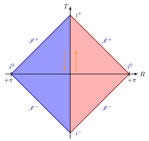
Figure 2: Minkowski spacetime conformal (Not Penrose) diagram that represents the DQFT construction with direct-sum vacuum (4.9) as discussed in Sec. 4. The left and right triangles are $\mathcal{P}\mathcal{T}$ conjugates of each other. The DQFT quantum field operator $\hat{\phi}$ is the direct-sum of $\hat{\phi}_{I},\hat{\phi}_{II}$ defined on the right and left, respectively, which follows from (4.3).

We now use the compactified coordinates (4.24) to draw a conformal (Not Penrose) diagram that represents DQFT construction (4.9), where we have an explicit $\mathcal{C}\mathcal{P}\mathcal{T}$  symmetry in quantization as discussed in Sec. (4). As depicted in Fig. 2, in DQFT construction, we split space into two parts by parity $\mathcal{P}$ transformation, therefore the right triangle in red denotes half of the space (region I) while the blue left triangle represents the remaining half (region II). The quantum states, in the whole spacetime, are a direct-sum of states $\hat{\phi}_{I}$, evolving forward in time (in the red triangle), and states $\hat{\phi}_{II}$ evolving backward in time (in the blue triangle). As a consequence of (4.5), we have

$$\left[\mathcal{O}_{I}\left(t,\,\textbf{x}\right),\,\mathcal{O}_{II}\left(-t^{\prime},\,-\textbf{x}^{\prime}\right)\right]=0\,.$$ (4.27)

Since we also demand (2.27) for the region I and II, we must have

$$\left[\mathcal{O}_{I}\left(x\right),\,\mathcal{O}_{I}(y)\right] =0,\quad\left(x-y\right)^{2}>0\,$$ (4.28)

$$\left[\mathcal{O}_{II}\left(x\right),\,\mathcal{O}_{II}(y)\right] =0,\quad\left(x-y\right)^{2}>0\,.$$

Therefore, as a consequence of (4.27) and (4.28), we satisfy both locality and causality requirements in DQFT.

We remind to the reader that Fig. 2 should not be confused with the standard Penrose diagram of Minkowski and should not be viewed as the two copies of Minkowski spacetime. Instead, the diagram fully represents Minkowski spacetime, where quantization is carried out considering a direct-sum vacuum structure. In addition, the full Minkowski spacetime discrete symmetries exist only when we take the direct-sum of regions I and II (the red and blue colored triangles). Due to conditions (4.27) and (4.28), we neither have a violation causality or any closed timelike curves.

5 Setting up quantization rules for curved spacetime (specifically for dS spacetime)

The goal of this section is to call the reader attention to key points and set up criteria for QFTCS formulation. Some of the points we discuss below are applicable to any curved spacetime, but our main focus in this manuscript is dS spacetime and we address other important curved spacetimes such as Schwarzchild BH in a subsequent paper [51].

• Whatever the curvature of spacetime is, it is legitimate to expect that in the high energy limit i.e., when the square of the KG field physical wave number exceeds the spacetime curvature, we must recover QFT in Minkowski spacetime.

• As a first step, to formulate a unitary QFT on curved spacetime, it is justifiable to assume some low curvature regime and then formulate QFTCS in such a way that we recover SQFT in relatively large energy limit, which doesn’t have to be Planck scale.

• It is most often assumed that understanding curved spacetime requires UV, especially Planck scale physics. We stress that this assumption might be too extreme. First of all, before we reach Planck scale distances we have to deal with curvature scales which are much below the Planck scales. In order to illustrate this, consider, for example, the curvature scale during inflation, or the very low curvature scale corresponding to the current acceleration of Universe, or the vast number of curvature scales of the plethora of differently sized BHs that exist in our Universe. Therefore, it might be justified that one must understand fully QFTCS before worrying about the full quantum gravity. In other words, unitary QFTCS is a first step to achieve in the quest for quantum gravity.

• An important point in QFTCS is to identify the discrete symmetries of a given spacetime and verify if it contains the $\mathcal{P}\mathcal{T}$ symmetry. Indeed, the most recent QFTCS studies, in dS spacetime, involve a careful account of discrete symmetries, especially the time reversal symmetry [52, 53, 54]. However, these studies explore the entanglement between different classical patches, of the disconnected (classical) spacetime regions, proposing a direct product of Hilbert spaces between gravitational and matter degrees of freedom. The way we setup QFT, in dS spacetime, is structurally very different and we are aiming to have a (quantum) spacetime description entirely based on pure states. Our construction is unitary with respect to individual degrees of freedom. In addition, our proposal is within the validity of peturbation theory.

• We claim that, even in curved geometry, there should always exist quantum states that evolve forward and backward in time. Time reversal is at the heart of quantum theory and we cannot give up this principle, because what we see in SQFT should be lifted to curved spacetime QFT. In nature, any general curved spacetime is connected to Minkowski spacetime, either through local Lorentz symmetry or via asymptotic limit or in the short distance (high energy) limit. In other words, if we have a curved spacetime (removing singular points) it is legitimate to think that ultra high energy particles would not see the spacetime curvature and they should behave according to the rules of SQFT. Therefore, it is essential to understand what is the role of time reversal over quantum states in a curved spacetime. Certainly, in a curved spacetime, time reversal physics may not be invariant like it is in SQFT. If there is a violation of $\mathcal{C}\mathcal{P}\mathcal{T}$  we should expect some sort of asymmetry in time reversal (quantum) physics. Our QFTCS formulation is build upon DQFT approach in Minkowski spacetime which will potentially take us towards a unitary QFTCS.

• We stress that our classical notion of time should not be mixed with the quantum mechanical one. Classical time, i.e., thermodynamic arrow of time. In the context of dS in FLRW coordinates the classical arrow of time corresponds to shrinking or growing size of the comoving Hubble radius.

• Quantum arrow of time can be matched with thermodynamical arrow of time when we impose initial conditions on quantum states. Therefore, we construct QFT in curved spacetime without worrying about the arrow of time for classical solutions. We can match our quantum arrow of time with the classical (thermodynamic) arrow of time selecting appropriate initial conditions on quantum states [20, 23].

• The notion of observer is not a well defined concept in a quantum theory [24]. Nevertheless, it is important according to theory of relativity. The notion of an observer defines the boundary, or a spacial region based on the horizon structure, of a given spacetime. The notion of observer is fixed once we specify the coordinate system. To formulate QFT in dS spacetime we restrict our approach to FLRW coordinate system. If one wants a corresponding QFT in a different coordinate system, we can use the so called Bogoliubov transformations [31]. In our formulation of QFTCS, we define an (imaginary) observer as someone for which there exist a horizon which is static or dynamical. For example, if the size of the horizon is fixed, for this (imaginary) observer, then the dS spacetime is static in nature and expressed in terms of the well known static coordinates. If, according to this (imaginary) observer, the size of the (comoving) horizon grows with time then it denotes a contracting Universe and if the (comoving) horizon shrinks with time he/she observes a expanding Universe. The imaginary observer’s clock only measures how the horizon size progresses and it has nothing to do with the time parameter in QFTCS.

• The appearance of an event or apparent horizon is the most important aspect of curved spacetime, at which quantum effects are expected to happen (for example de Sitter or BH spacetime). A unitary formulation of QFT is required to satisfy an essential feature that the imaginary observer should have complete information about the (quantum) physics happening within the horizon described by pure states. This is known as the observer complementarity principle that is often quoted in several studies [30]. Existence of an horizon, in curved spacetime, leads to the so called information loss problem (being a serious problem both in the context of dS and BH physics), according to the standard intuitive methods of field quantization in curved spacetime. Although the occurrence of the information problem already appears when we semiclassically quantize a field, the resolution to that problem is majorly addressed in the context of an unknown theory of quantum gravity. Our attempt is based on questioning every step in the construction of a QFTCS [26].

• The final point, we would like to make, is that to understand QFT in any realistic curved spacetime one has to learn how to deal with horizons. Without this step, the progress we can make towards formulating a consistent quantum gravity theory is expected to be very difficult.

6 Direct-sum Fock space construction of QFT in de Sitter spacetime

After Minkowski spacetime, the physically most relevant maximally symmetric spacetime is dS. The dS metric exhibits the presence of event or apparent horizons, depending on the coordinate system we choose to represent it. As such, it is most often said that the (quantum) physics in dS spacetime is observer dependent [55]. This makes dS spacetime QFT more challenging compared to another maximally symmetric spacetime called Anti-dS (AdS). Unlike dS, AdS spacetime does not have horizons and it is the only curved spacetime where S-matrix formulation is claimed to be understood [56, 57], despite the existence of open problems that are yet to be addressed [58]. Due to the deeper understanding of the AdS/CFT correspondence, QFT in dS is mainly addressed from the holographic point of view [59] or using the so-called entanglement between various (classical) regions of spacetime [60, 54, 61, 53]. However, there are two questions involved here. The first question is: what are the rules of quantization in dS spacetime, which should be addressed within the validity of perturbation theory? and this question actually seeks for understanding how to put together gravity and quantum mechanics. The second question is: how one can end up with a dS spacetime starting from the grand framework of quantum gravity? which has mainly been the subject of investigation within the scope of string theory for several decades [62]. Our efforts are directed to find an answer to, or at least a consistent route to answer, the first question, which we think will ultimately be helpful to attack the second grand question. Surely, we greatly acknowledge the weight of the second question, but we stress that it is beyond the scope of this paper.

Without further delay, let us turn to the main subject of this section, where our aim is to apply a set of new quantization rules to de Sitter (dS) spacetime. Those will play a vital role in our understanding of cosmology. The success of inflationary cosmology is a consequence of the spontaneous breaking of de Sitter symmetry [63]. The dS QFT construction, considered here, is different from the standard textbook picture [26, 31], because as it is well-known that dS SQFT does lead to inconsistencies in relation with unitarity (evolution of pure states into mixed states) and information loss [30]. Another important issue of dS SQFT is that one can only define either in states or out states which forbids us to define a consistent scattering problem. Nevertheless, several developments were proposed following an unknown theory of quantum gravity, or based on entanglement between unknown Universes, despite admitting the lack of an S-matrix formulation in dS space [62, 16, 64, 65, 66, 60, 67, 68, 69]. The story of (quantum) troubles with dS spacetime [67] is not really an issue raised in recent years, but rather started from the days of Schrödinger. Indeed, he already pointed out that dS spacetime does have ambiguities, which turn into a serious obstacle to construct a reasonable quantum theory [29]. Schrödinger’s monograph named Expanding Universes [29] points to the non-existence global arrow of time or, in other words, the problem of the lack of a Cauchy surface in dS spacetime which hamper a correct quantum theory formulation. Schrödinger proposed that one must carry with the so-called antipodal identification of the points in spacetime, to define one Universe with a unique arrow of time and a well defined Cauchy surface. This Schrödinger view is known as Elliptic dS, and it has been explored to define a dS unitary QFT [70, 30]. However, the idea of Elliptic dS space fails to give a consistent QFTCS due to the possibility of closed time like curves occurence, if one take a departure from dS spacetime [71]. Nevertheless, Schödinger monograph provides inspiring ideas, such as about distinguishing the notions of time classically and quantum mechanically, which we strongly envisage as the key for formulating QFTCS. Furthermore, Schrödinger proposes that any observer should have complete information within his/her own horizon, which in modern language translates to the description of Universe within the horizon using so-called pure states. We take this as a guiding principle in the present work.

The dS manifold is characterized by its simple relations to the metric tensor, such as follows

$$R^{\mu}_{\nu\rho\sigma}=\frac{R}{12}\left(\delta^{\mu}_{\rho}g_{\nu\sigma}-\delta^{\mu}_{\sigma}g_{\nu\rho}\right),\quad R_{\nu\sigma}=\frac{R}{4}g_{\nu\sigma},\quad R=\mathrm{const}\,.$$ (6.1)

The above definition is coordinate independent and, as it is well-known, dS spacetime is a solution of Einstein’s GR with a cosmological constant. The question we address, in the context of dS spacetime in a given coordinate system, is how can we quantize a free KG field, and how do we use the understanding of free fields in that spacetime, to define a notion of scattering if we include the interactions perturbatively. However, we surely ignore here the quantum fields back reaction on the dS geometry and also leave the questions of whether dS is stable or not, and if one does require to understand (quantum) gravity at non-perturbative level (See [72] for more discussion on these topics). We strongly acknowledge the later questions are legitimate, but we strictly limit ourselves to QFTCS rather than quantum gravity. Below we present our analysis for dS QFT, expressed in FLRW coordinates. Part of what we will discuss can also be found in a previous work [23]. Therein, we extract observational consequences of applying QFTCS, with direct-sum Fock space, in the context of single field inflationary cosmology addressing one of the prominent CMB anomaly called the Hemispherical power asymmetry. In other words, direct-sum QFTCS (shortly DQFTCS) allow us to make a prediction, which can be tested with future CMB and Primordial Gravitational Waves (PGWs) observations. The purpose, in this paper, is to give further theoretical ground and take a step towards the understanding of unitarity and S-matrix in QFTCS.

6.1 Discrete spacetime transformations for the QFT in flat and closed dS

Let us consider dS metric in flat FLRW coordinates, which are widely used in the context of inflationary cosmology.

$$ds^{2}=-dt^{2}+a(t)^{2}d\textbf{x}^{2}$$ (6.2)

where the scale factor is given by

$$a(t)=e^{Ht},\quad H^{2}=\left(\frac{1}{a}\frac{da}{dt}\right)^{2}>0\,,$$ (6.3)

where $H$ here is the Hubble parameter. Each point in dS is surrounded by a horizon, given by the coordinate radius or also known as the comoving Hubble radius [73].

$$r_{H}=\Big{|}\frac{1}{aH}\Big{|}$$ (6.4)

In order to understand quantization, in dS spacetime, it is convenient to write dS metric (6.2) in terms of the conformal time, defined by

$$d\tau=-\frac{dt}{a(t)}\,.$$ (6.5)

Integrating this equation, we obtain

$$\tau=\frac{1}{a(t)H}\,\text{,}$$ (6.6)

where the integration constant is set to zero, the scale factor then reads

$$a(\tau)=\frac{1}{H\tau}\,\text{.}$$ (6.7)

In terms of this new time coordinate $\tau$, the dS metric is conformal to Minkowski metric

$$ds^{2}=\frac{1}{H^{2}\tau^{2}}\left(-d\tau^{2}+d\textbf{x}^{2}\right)$$ (6.8)

In terms of $\tau$, metric (6.8) becomes conformal to Minkowski and provide a huge advantage for quantizing the KG field. Because, unless we write the metric as (6.8), we cannot rewrite the effect of the curved spacetime in terms of the harmonic oscillator formalism, which is the only one we know how to quantize.

Note that the time coordinate $\tau\gtrless 0$, has a coordinate singularity at $\tau=0$. Nevertheless, it is just an artifact of the coordinate transformation, in reality there is no spacetime singularity as such. We can clearly see that the dS metric satisfies $\mathcal{P}\mathcal{T}$ symmetries just like Minkowski spacetime

$$\mathcal{P}\mathcal{T}:\tau\to-\tau,\quad\textbf{x}\to-\textbf{x}\,.$$ (6.9)

We perform quantization and take the conformal coordinate $\tau$ as a time parameter in quantum theory. We can notice that the time ($\tau$) reflection operation actually leads to time reversal in cosmic time, as well as the change of sign for the Hubble parameter $H$.

$$\mathcal{T}:\tau\to-\tau\implies t\to-t,\,H\to-H\,.$$ (6.10)

It is really worth noting that $H\to-H$ operation does not change any dS curvature invariant. For example, the dS Ricci scalar $R=12H^{2}$ is completely symmetric under the change of sign in $H$. As we extensively discussed in sections 2, 3 and 4, discrete spacetime transformations play a crucial role in the QFT formulation. Thus, before we go for dS QFT, we notice that dS discrete symmetries comes with the additional (quantum mechanical) parameter $H$, along with time which is already a parameter in quantum theory.

One simple observation, we can make from (6.2), is that we have an

$${\rm expanding\,Universe:}\implies\begin{cases}t:-\infty\to+\infty,\quad H>0&(\tau:+\infty\to 0)\\ t:+\infty\to-\infty,\quad H<0&(\tau:-\infty\to 0)\end{cases}$$ (6.11)

and a

$${\rm contracting\,Universe:}\implies\begin{cases}t:+\infty\to-\infty,\quad H>0&(\tau:0\to+\infty)\\ t:-\infty\to+\infty,\quad H<0&(\tau:0\to-\infty)\end{cases}$$ (6.12)

Expansion, and contraction, of the universe is now determined by the conformal time $\tau$ flow:

$$\text{Expansion: }\tau:\pm\infty\longrightarrow 0\,\,(r_{H}\,\,{\rm shrinks})\,\text{,} \text{Contraction: }0\longrightarrow\pm\infty\,\,(r_{H}\,\,{\rm grows})\,,$$ (6.13)

rather than by the sign of $H$. In the literature it is often assumed that $H>0$ indicates expanding Universe [74, 75, 68, 76] but, as we argue, $H$ is also a parameter in quantum theory and its sign is relevant in conjunction with time. Notice that the time reversal operation does not change the nature of the Universe, i.e., an expanding Universe remains expanding and contracting Universe remains contracting ((6.11) and (6.12)). In the literature it is generally assumed that these the two expanding branches, or the two contracting branches, are separate Universes. But we remind the reader that from the quantum mechanical point of view, time reversal operation cannot have any classical analog. We adopt the notion that an expanding Universe is defined by its shrinking comoving horizon and that the arrow of time is an irrelevant concept. However, if we have both time directions in quantum theory, we keep locality and causality through the way we impose commutation relations for the operators.

Let us consider dS space expressed in terms of the closed FLRW coordinates, which are also known as the global coordinates [75, 77].

$$ds^{2}=-dt^{2}+\cosh^{2}\left(Ht\right)\left[d\chi^{2}+\sin^{2}\chi d\Omega^{2}\right]\,,$$ (6.14)

where $0\leq\chi=\frac{\sin^{-1}\left(\sqrt{6}Hr\right)}{\sqrt{6}H}\leq\pi$. The above metric Ricci scalar is $R=12H^{2}$. This metric describes the contraction and expansion of a 3-dimensional sphere. For quantization purposes, it is useful to write metric (6.14) in a Minkowski spacetime conformal form by defining conformal time as

$$\tau=\int\frac{dt}{a(t)}=\frac{2}{H}\tan^{-1}\left(\tanh\left(\frac{Ht}{2}\right)\right)\,.$$ (6.15)

The metric, in terms of this conformal time, takes the form

$$ds^{2}=\frac{1}{\cos^{2}\tau}\left[-d\tau^{2}+d\chi^{2}+\sin^{2}\chi d\Omega^{2}\right]$$ (6.16)

The metric (6.16) discrete symmetries are

$$\mathcal{P}\mathcal{T}:\tau\to-\tau,\quad\chi\to\chi,\quad\left(\theta,\,\varphi\right)\to\left(\pi-\theta,\,\varphi+\pi\right)\,.$$ (6.17)

As for flat FLRW dS, the time reversal operation involves flipping the sign of $H$. This means

$${\rm contraction\,to\,expansion}\implies\begin{cases}t:-\infty\to+\infty,\quad H>0,\quad\left(\tau:-\frac{\pi}{2}\to\frac{\pi}{2}\right)\\ t:+\infty\to-\infty,\quad H<0,\quad\left(\tau:\frac{\pi}{2}\to-\frac{\pi}{2}\right)\end{cases}$$ (6.18)

Therefore, even in dS global coordinates, the sign of $H$ plays a crucial role in the QFT formulation. We emphasize that the time reversal operation, considered here, is a purely quantum mechanical concept, which has no classical analog (See [78, 79] for more discussions about the quantum mechanical concept of time). Therefore (6.18) represents one Universe which is evolving from contraction to expansion, the discrete transformation applied from the first to the second line of (6.18) is exactly what we call time reversal operation in closed dS.

6.2 Direct-sum QFT in dS

After reviewing dS spacetime, expressed in flat and closed FLRW coordinates, let us step into the subject KG field quantization in dS spacetime. Our approach consist in applying a similar procedure as for the DQFT framework, that we discussed in Sections 4 and 4.1 in the context of Minkowski spacetime. At this point, we consider DQFT quantization in flat (expanding) FLRW dS spacetime (6.11) and a similar procedure can be followed, using discrete spacetime transformations, for closed dS according to (6.17) and (6.18).

The action of a massless scalar field in dS (flat FLRW case) is given by

$$S_{\phi}=-\frac{1}{2}\int d\tau d^{3}xa^{2}\phi\left(\partial_{\tau}^{2}+2\mathcal{H}\partial_{\tau}+k^{2}\right)\phi\,,$$ (6.19)

where $\mathcal{H}=\frac{1}{a}\frac{da}{d\tau}=aH$. We can verify that the above action is invariant under the $\mathcal{P}\mathcal{T}$ transformation, defined in (6.9). In order to implement quantization, it is convenient to rescale the field $\phi\to a\phi$, which allows to define the following action

$$S_{\phi}=\frac{1}{2}\int d\tau d^{3}x\Big{[}\phi^{\prime 2}-\left(\partial_{i}\phi\right)^{2}-\frac{2}{\tau^{2}}\phi^{2}\Big{]}\,.$$ (6.20)

The above action seems to describe a KG field, in flat space time, with a time dependent mass. Under this circumstance, we know how to quantize the KG field, by following a procedure similar to the one employed in Sec. 4.

When we quantize this scalar field, we propose that the scalar field operator $\hat{\phi}\left(\tau,\,\textbf{x}\right)$ is now a direct-sum of the field operators as

$$\hat{\phi}\left(\tau,\,\textbf{x}\right)=\frac{1}{\sqrt{2}}\hat{\phi}_{I}\left(\tau,\,\textbf{x}\right)\oplus\frac{1}{\sqrt{2}}\hat{\phi}_{II}\left(-\tau,\,-\textbf{x}\right)=\frac{1}{\sqrt{2}}\begin{pmatrix}\hat{\phi}_{I}\left(\tau,\,\textbf{x}\right)&0\\ 0&\hat{\phi}_{II}\left(-\tau,\,-\textbf{x}\right)\end{pmatrix}\,.$$ (6.21)

where

$$\hat{\phi}_{I}\left(\tau,\,\textbf{x}\right) =\frac{1}{\left(2\pi\right)^{3/2}}\int d^{3}k\Bigg{[}\hat{c}_{I\,\textbf{k}}{\phi}_{I\,k}\left(\tau\right)e^{-i\textbf{k}\cdot\textbf{x}}+\hat{c}_{I\,\textbf{k}}^{\dagger}{\phi}^{\ast}_{I\,k}\left(\tau\right)e^{i\textbf{k}\cdot\textbf{x}}\Bigg{]}\,$$ (6.22)

$$\hat{\phi}_{II}\left(-\tau,\,-\textbf{x}\right) =\frac{1}{\left(2\pi\right)^{3/2}}\int d^{3}k\Bigg{[}\hat{c}_{II\,\textbf{k}}{\phi}_{-\,k}\left(-\tau\right)e^{i\textbf{k}\cdot\textbf{x}}+\hat{c}_{II\,\textbf{k}}^{\dagger}{\phi}^{\ast}_{II\,k}\left(-\tau\right)e^{-i\textbf{k}\cdot\textbf{x}}\Bigg{]}\,$$

Notice that the creation and annihilation operators $\hat{c}_{\pm\textbf{k}},\,\hat{c}^{\dagger}_{\pm\textbf{k}}$ satisfy the following commutation relations (which are very similar to (4.5))

$$=[\hat{c}_{II\,\textbf{k}},\,\hat{c}_{II\,\textbf{k}^{\prime}}^{\dagger}]=\delta^{(3)}\left(\textbf{k}-\textbf{k}^{\prime}\right)$$ (6.23)

$$[\hat{c}_{I\,\textbf{k}},\,\hat{c}_{II\,\textbf{k}^{\prime}}] =[\hat{c}_{I\,\textbf{k}},\,\hat{c}_{II\,\textbf{k}^{\prime}}^{\dagger}]=[\hat{c}_{I\,\textbf{k}}^{\dagger},\,\hat{c}_{II\,\textbf{k}^{\prime}}^{\dagger}]=0\,.$$

Consequently, we also have

$$=i\delta\left(\textbf{x}-\textbf{x}^{\prime}\right)$$ (6.24)

$$[\hat{\phi}_{II}\left(-t,-\textbf{x}\right),\,\pi_{II}\left(-t,\,-\textbf{x}^{\prime}\right)] =-i\delta\left(\textbf{x}-\textbf{x}^{\prime}\right)$$

$$\left[\hat{\phi}_{I}\left(\tau,\,\textbf{x}\right),\,\hat{\phi}_{II}\left(-\tau,\,-\textbf{x}\right)\right] =0\,,$$

where

$$\pi_{I}\left(\tau,\,\textbf{x}\right)=\partial_{\tau}\phi_{I},\quad\pi_{II}\left(-\tau,\,-\textbf{x}\right)=-\partial_{\tau}\phi_{II}\,.$$ (6.25)

The third line of (6.24) is consistent with quantum theory locality principle. It is true for any operator in region I and region II of dS spacetime

$$\left[\mathcal{O}_{I}\left(\tau,\,\textbf{x}\right),\,\mathcal{O}_{II}\left(-\tau^{\prime},\,-\textbf{x}^{\prime}\right)\right]=0\,.$$ (6.26)

It is easy to see (6.26) is analogous to the one of DQFT in Minkowski spacetime (4.27).

In flat FLRW dS as the Universe expands, modes exit the horizon at spacelike separated points. According to our description, the mode exiting the horizon at one side fixes the state exiting at the other side, but without violating the locality principle guaranteed by the commutation relations. We shall discuss this further in the later section.

Functions $\phi_{I\,k},\,\phi_{II\,k}$ are defined as

$$\phi_{I,\,k} =\alpha_{I\,k}\frac{e^{ik\tau}}{\sqrt{2k}}\left(1+\frac{i}{k\tau}\right)+\beta_{I\,k}\frac{e^{-ik\tau}}{\sqrt{2k}}\left(1-\frac{i}{k\tau}\right)\,,$$ (6.27)

$$\phi_{II,\,k} =\alpha_{II\,k}\frac{e^{-ik\tau}}{\sqrt{2k}}\left(1-\frac{i}{k\tau}\right)+\beta_{II\,k}\frac{e^{ik\tau}}{\sqrt{2k}}\left(1+\frac{i}{k\tau}\right)\,,$$

satisfying $\phi_{I,\,k}\Big{|}_{\mathcal{T}:\,\tau\to-\tau}=\phi_{II,\,k}$ and are obtained by solving the Mukhanov-Sasaki equation [23]

$$\phi_{m\,k}^{\prime\prime}+\left(k^{2}-\frac{2}{\tau^{2}}\right)\phi_{m\,k}=0\,.$$ (6.28)

where $m=I,\,II$. We can notice, from (6.28), that in the limit $k^{2}\gg 2/\tau^{2}$ or $k^{2}\gg 2/r_{H}^{2}$, i.e., when the wavelength of the mode is much less than the size of the comoving horizon $r_{H}$, we recover DQFT results discussed in Sec. 4. Therefore, we fix the Bogoliubov coefficients as $\left(\alpha_{I\,k},\,\beta_{I\,k}\right)=\left(\alpha_{II\,k},\,\beta_{II\,k}\right)=\left(1,\,0\right)$, which are compatible with the Wronskian conditions $\phi_{I,\,k}\phi^{\prime\ast}_{I,\,k}-\phi^{\ast}_{I,\,k}\varphi^{\prime}_{I,\,k}=i$ and $\phi_{II,\,k}\phi^{\prime\ast}_{II,\,k}-\phi^{\ast}_{II,\,k}\phi^{\prime}_{II,\,k}=-i$, that corresponds to the canonical commutation relations (6.24).

The dS spacetime vacuum is given by the direct sum

$$|0\rangle_{dS}=|0\rangle_{dSI}\oplus|0\rangle_{dSII}=\begin{pmatrix}|0\rangle_{dSI}\\ |0\rangle_{dSII}\end{pmatrix}\,.$$ (6.29)

where $|0\rangle_{dSI},\,|0\rangle_{dSII}$ are defined according to

$$\hat{c}_{I\,\textbf{k}}|0\rangle_{dSI}=0,\quad\hat{c}_{II\,\textbf{k}}|0\rangle_{dSII}=0$$ (6.30)

The choice $\left(\alpha_{I\,k},\,\beta_{I\,k}\right)=\left(1,\,0\right)=\left(\alpha_{II\,k},\,\beta_{II\,k}\right)$ translate into vacuums $\hat{\phi}_{I}\left(\tau,\,\textbf{x}\right)|0\rangle_{dSI}$, $\hat{\phi}_{II}\left(\tau,\,\textbf{x}\right)|0\rangle_{dSII}$, which correspond, respectively, to positive and negative frequencies solutions in the limits $\tau\to\pm\infty$. We emphasize that the limits $\tau\to\pm\infty$ can also be viewed as the limit when $k^{2}\gg 2/\tau^{2}$, which is nothing but the local Minkowski limit. Therefore, in this limit, dS spacetime DQFT should exactly reduce to Minkowski spacetime DQFT (See Sec. 4 4).

Notice that, in dS DQFT framework, we divide the spatial part of dS expanding Universe (6.11) into two parts, $dSI$ and $dSII$, through the parity transformation, and then we associate opposite time evolutions to states in region $dSI$ ($\tau:+\infty\to 0$) and $dSII$ ($\tau:-\infty\to 0$). The direct sum of these states represent the full (quantum mechanical) evolution of the scalar field in the direct sum vacuum which describes the whole dS spacetime. We argue that there is only a single degree of freedom, which is represented as the direct sum of two complementary parts. In addition, we have that dS spacetime DQFT is $\mathcal{C}\mathcal{P}\mathcal{T}$  symmetric. We can verify this, observing that

$$\frac{1}{a^{2}}{}_{dSI}\langle 0|\hat{\phi}_{I}\left(\tau,\,\textbf{x}\right)\hat{\phi}_{I}\left(\tau,\,\textbf{x}^{\prime}\right)|0\rangle_{dSI}=$$ (6.31)

$$\frac{1}{a^{2}}{}_{dSII}\langle 0|\hat{\phi}_{II}\left(-\tau,\,-\textbf{x}\right)\hat{\phi}_{II}\left(-\tau,\,-\textbf{x}^{\prime}\right)|0\rangle_{dSII}=\frac{H^{2}}{4\pi^{2}k^{3}}\,.$$

We see that (6.31), analogous to the result of Minkowski spacetime DQFT (4.15), implies that the correlations of quantum fields related by $\mathcal{P}\mathcal{T}$ transformations are identical in the case of dS spacetime. This indicates that this dS spacetime QFT formulation might be $\mathcal{P}\mathcal{T}$ or $\mathcal{C}\mathcal{P}\mathcal{T}$ (if we include charged fields) symmetric. The obvious question, at this point, is related to the scattering problem and how dS DQFT enable us to define an S-matrix, which is thought to be an impossible task to achieve for dS spacetime [16]. We propose to analyse this question in the following.

6.3 Unitarity and observer complementarity in dS DQFT

One of the issue with dS spacetime is the way it challenges us with unitarity violation, for example, with the evolution of pure states into the mixed states. In addition, the thermodynamic point of view that emerges with the finiteness of entropy, which lead to the suggestion of Hilbert space finiteness [80, 81, 82]. At the fundamental level, all these troubling issues emerge from the fact that we do not know how to reconstruct what is beyond the observer’s horizon. One of the resolution to the problem is the proposal of dS spacetime observer complementarity [82],, which states that all observers are equivalent (no one should see any violation of unitarity) and all the information is contained within each observer horizon. This is known as the central dogma in dS, which is mainly explored in the context of static dS in string theory and AdS/CFT [85]. We aim to address the above issues from the point of view of dS DQFT.

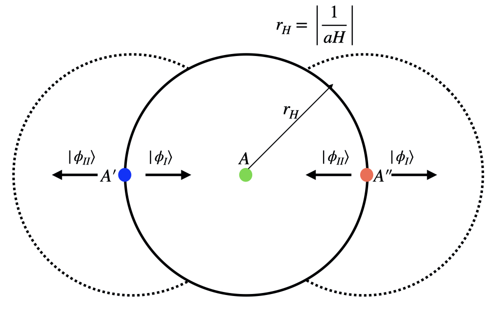
Figure 3: This figure illustrates three comoving (imaginary) observers $A,\,A^{\prime},\,A^{\prime\prime}$ with the corresponding comoving horizon radius $r_{H}=|\frac{1}{aH}|$ at a moment of dS expansion. We have suppressed here the angular coordinates $\left(\theta,\,\varphi\right)$. Points $A^{\prime}$ and $A^{\prime\prime}$ are on the horizon of $A$ at opposite sides of the horizon, that are spacelike separated, i.e., at the angles $\left(\theta,\,\varphi\right)$ and $\left(\pi-\theta,\,\pi+\varphi\right)$ respectively. The dotted circles with the same $r_{H}$ represent the respective comoving horizons of $A^{\prime}$ and $A^{\prime\prime}$. In the figure, $|\phi_{I}\rangle,\,|\phi_{II}\rangle$ are defined in (6.32).

First of all, the comoving horizon (6.4) is the most important quantity attached to dS spacetime. We represent it in Fig. 3, where we take an (imaginary) observer $A$ with $r_{H}$ at a moment of dS expansion, and two other imaginary observers $A^{\prime},\,A^{\prime\prime}$ on the horizon of $A$. Expanding dS Universe would translate in a shrinking of the comoving horizon size, as the scale factor grows according to the thermodynamic concept of time. In the framework of dS DQFT we divide space into two halves, related by parity transformation, and associate (quantum mechanical) time evolution to the direct-sum state in the direct-sum Fock space (6.29). This represents a single degree of freedom (following from (6.21)) in the entire two spatial regions, which span points of $\left(\theta,\,\varphi\right)$ and $\left(\pi-\theta,\,\pi+\varphi\right)$ within the comoving radius $r_{H}$. In Fig. 3, $|\phi_{I}\rangle=\hat{c}_{I\,\textbf{k}}^{\dagger}|0\rangle_{dSI}$ and $|\phi_{II}\rangle=\hat{c}_{II\,\textbf{k}}^{\dagger}|0\rangle_{dSII}$ form the direct sum state

$$|\phi\rangle =\left(\hat{c}^{\dagger}_{I\,\textbf{k}}\oplus\hat{c}^{\dagger}_{II\,\textbf{k}}\right)|0\rangle_{dS}$$ (6.32)

$$=\frac{1}{\sqrt{2}}\begin{pmatrix}\hat{c}^{\dagger}_{I\,\textbf{k}}&0\\ 0&\hat{c}^{\dagger}_{II\,\textbf{k}}\end{pmatrix}\begin{pmatrix}|0\rangle_{dSI}\\ |0\rangle_{dSII}\end{pmatrix}$$

$$=\frac{1}{\sqrt{2}}|\phi_{I}\rangle\oplus\frac{1}{\sqrt{2}}|\phi_{II}\rangle=\frac{1}{\sqrt{2}}\begin{pmatrix}|\phi_{I}\rangle\\ |\phi_{II}\rangle\end{pmatrix}\,.$$

By construction, in dS DQFT, which we established in Sec. (6.2) and (6.21), the imaginary observer $A$ always witness the direct sum state (6.32) within his (comoving) horizon and, as we can see from Fig. 3, the two imaginary observers at $A^{\prime}$ and $A^{\prime\prime}$ also have the same state within their horizon radius $r_{H}$. This implies that, by observing the direct sum state (6.32), imaginary observer $A$ can reconstruct what is happening beyond his/her horizon. Thus, we account for the observer complementarity principle and every observer experience the same physics, in the sense that there will not be any evolution of pure states to mixed states which is the problem according to the standard textbook description of QFTCS.

In Fig. 3 we can see that, even though the imaginary observers $A^{\prime}$ and $A^{\prime\prime}$ are spacelike separated, $A^{\prime\prime}$ by finding the state $|\phi_{I}\rangle$ in the right hand side can deduce what $A^{\prime}$ would find on its left hand side. This implies $A^{\prime\prime}$ can accurately deduce what $A^{\prime}$ can access. This has profound implications for the understanding of dS spacetime. It has been recently pointed out that the deepest problem in understanding quantum & gravity is violation of unitarity at distances much larger than Planck scales and it is also argued that the challenge for QFTCS is the conflict between quantum mechanics, relativity and locality. To resolve the conundrums it has been speculated that the nonlocality via quantum entanglement and direct-product Hilbert space would play a crucial role in formulating QFTCS [8]. Here we argue that a unitary QFTCS only requires a new concept of (local) time which is a parameter and an additional condition to the usual definition of locality is required (See (4.27) and (6.26)). Our QFA approach is exactly based on the fact that there is no global definition of time in curved spacetime. Therefore, we completely rely on the discrete spacetime transformations, whenever one goes from one spatial region to another by parity $\textbf{x}\to-\textbf{x}$ we apply time reversal to the quantum states by changing the Fock space. The two Fock spaces direct-sum form the full description of a quantum state within the observable space associated with an imaginary observer. Indeed, according to (6.32) a quantum state $|\phi\rangle$ actually mean, $|\phi_{I}\rangle$ at position x evolves forward in time and $|\phi_{II}\rangle$ at position $-\textbf{x}$ evolves backward in time like they are two sides of the same coin. This can be generalized to multiparticle states as well following (4.10) and (6.29). For example, let us consider usual two particle states with tensor product of Hilbert spaces, in the direct-sum formulation it can be expressed as

$$\mathcal{H}_{P} =\mathcal{H}_{dS1}\otimes\mathcal{H}_{dS2}$$ (6.33)

$$=\left(\mathcal{H}_{dSI1}\oplus\mathcal{H}_{dSII1}\right)\otimes\left(\mathcal{H}_{dSI2}\oplus\mathcal{H}_{dSII2}\right)$$

$$=\left(\mathcal{H}_{dSI1}\otimes\mathcal{H}_{dSI2}\right)\oplus\left(\mathcal{H}_{dSII1}\otimes\mathcal{H}_{dSII2}\right)\,,$$

where we can see the two particle tensor product Hilbert space is $\mathcal{P}\mathcal{T}$ symmetric and two particle entanglement splits into direct-sum of tensor products of Hilbert spaces in region $dSI$ and region $dSII$ respectively. This DQFT prescription by construction encodes fully the (quantum) information beyond the horizon to within the horizon in a way an observer does not lose anything beyond his/her horizon. This is solely due to the DQFT construction where an additional locality condition (6.26) is implemented. As we can see in Fig. 3, the imaginary observer $A$ sees the combination of both $|\phi_{I}\rangle$ and $|\phi_{II}\rangle$ forming the full direct-sum state $|\phi\rangle$ which is a pure state. On the right hand side of $A$, even though $|\phi\rangle_{I}$ going out of the horizon, the imaginary observer $A$ is not loosing anything as he/she got to receive it from the left hand side. At the first sight, it may appear to be duplication of information/cloning but it is absolutely not because no observer can see the same information twice within his/her observable horizon. Therefore, we definitely satisfy the so-called no cloning theorem in quantum theory. This imply all the imaginary observers in dS spacetime in the context of DQFT are equivalent although not identical. The DQFT framework in static dS spacetime will be discussed along with QFT in Schwarzchild spacetime in the companion paper [51].

6.4 S-matrix and conformal (Not Penrose) diagram of dS DQFT

One important aim of QFTCS, and quantum gravity, is to describe scattering and compute amplitudes involving all gravitational and matter degrees of freedom. To achieve this, the first step is to understand semiclassically how to quantize a scalar field and describe the interactions perturbatively, neglecting back reactions. Unless we do this step, the ultimate goal is always distant. As we discussed before, if we go to a sufficiently high energy limit, we should recover Minkowski QFT. It serves to verify if our approach to QFTCS is on the right track. To make progress, within this setup, we choose to ignore, for the momen,t all the popular claims about S-matrix in dS spacetime and/or dS cosmology [16, 74, 62, 64]. Those claims are stemmed upon numerous classical notions, before carrying quantization, and also based on hidden beliefs in the particularly popular frameworks of quantum gravity.

As we discussed in Sec. 6.2, in the sub-horizon limit $k^{2}\gg\frac{2}{\tau^{2}}$, we expect to recover Minkowski limit. This should be understood in two ways. First of all, any mode is sub-horizon in the sufficient past i.e., $a\to 0$ as $\tau\to\pm\infty$. As we noted before Sec. 6.1, the sign of $\tau$ does not determine spacetime, since dS metric (6.16) is precisely time symmetric. Secondly, at any given moment of dS expansion (i.e., at any value of $a$) we can always have modes that are sub-horizon. These are the two perspectives that are really important to understand the problem of scattering in dS. The regular meaning of asymptotic states in the context of SQFT or DQFT are bound to take a slightly different meaning in the context of dS spacetime.

Contrary to the popular expectations against existence of a dS S-matrix [16], here we argue otherwise. From the metric (6.2) we can notice that, in the time scales $\ll\frac{1}{|H|}$, the curvature effects can be negligible and scattering can be completely treated like it is in Minkowski. In the limit where interactions involve high energy modes, within the time scales $\ll\frac{1}{|H|}$, the dS spacetime S-matrix should reduce to Minkowski spacetime S-matrix. This reasoning ensures the existence S-matrix in dS and in fact the same reasoning can be applied to any curved spacetime.

Imagine now that we have a particular set of modes that are all sufficiently sub-horizon (i.e., $k^{2}\gtrsim a^{2}H^{2}$, such that we cannot completely neglect the background curvature) when they scatter. In the sufficient infinite past, we can treat them as modes that are more deep inside the horizon (i.e., $k\gg a^{2}H^{2}$ at which we completely neglect the background curvature effects and where they are very similar to Minkowski spacetime modes). At sufficient future all the modes that scatter in the near sub-horizon, become long wavelength modes i.e., super-horizon $k^{2}\ll a^{2}H^{2}$ and act as free non-interacting states. After the modes become super-horizon it is expected that they evolve classically rather than quantum mechanically. This has been proposed in multifield inflation studies (See [86] and references therein for further details).

As a toy model example, we consider two interacting KG fields given by

$$S_{\rm KGs}=\int\sqrt{-g}d^{4}x\left[\phi\square\phi+\chi\square\chi-g^{2}\chi\phi^{2}\right]\,,$$ (6.34)

where $g$ is the coupling constant. As we discussed before, we quantize fields in dS after transforming them into harmonic oscillators, by rescaling the fields $\phi\to a\phi,\,\chi\to a\chi$ which implies

$$S^{\rm conformal}_{\rm KGs}=\int d\tau d^{3}x\left[\phi\square_{\tau}\phi+\chi\square_{\tau}\chi-g_{\rm eff}^{2}\chi\phi^{2}\right]\,,$$ (6.35)

where $\square_{\tau}=\left(\partial_{\tau}^{2}+k^{2}-\frac{2}{\tau^{2}}\right)$ and $g_{\rm eff}=\sqrt{a}g$ is the effective coupling constant which naturally becomes smaller as $a\to 0$. The action (6.35), in terms of the effective gravitational interaction $g_{\rm eff}$, is supposed to describe the scattering problem in dS at time scales $\Delta t\sim\frac{1}{|H|}$. If the scattering involves high energy modes, where all the modes remain deep inside the horizon all the way from beginning to the end, and if $\Delta t\ll\frac{1}{|H|}$, then for practical purposes the background curvature effects can be dropped through the rescaling $a\to 1$ and $g_{\rm eff}\to g$.

We present our expected picture for dS scattering in Fig. 4.

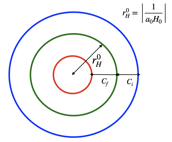
Figure 4: We depict the scattering process schematic picture in expanding dS. Here $r_{H}^{0}$ denotes the scale at which the modes start to interact and undergo scattering. In the sufficient past (i.e., when the comoving horizon was $r_{H}=r_{H}^{0}+C_{i}$ where $C_{i}$ is some arbitrary constant radius) we assume the modes are sufficiently sub-horizon and non-interacting. Whereas in the sufficient future (i.e., when the comoving horizon will be $r_{H}=r_{H}^{0}-C_{f}$ where $C_{f}$ is some arbitrary constant radius) we assume that the modes, after scattering, exit beyond radius $r_{H}^{0}$ and become classically evolving fluctuations.

Action (6.35) seems to decribe two interacting scalar fields in flat spacetime, with time ($\tau$) dependent masses and coupling constant $g_{\rm eff}$. At this point, and taking into account Fig. 4, we can now write a dS DQFT S-matrix in analogy with (4.12) and (4.13) as

$$S_{dS}=S_{dSI}\oplus S_{dSII}$$ (6.36)

where

$$S_{dSI}=T_{dSI}\Bigg{\{}e^{-i\int_{-r_{H}^{0}-C_{i}}^{-r_{H}^{0}+C_{f}}H_{int}\,\,d\tau}\Bigg{\}},\quad S_{dSII}=T_{dSII}\Bigg{\{}e^{i\int_{r_{H}^{0}+C_{i}}^{r_{H}^{0}-C_{f}}H_{int}\,\,d\tau}\Bigg{\}}$$ (6.37)

with $T_{dSI},\,T_{dSII}$ representing the time orderings attached to the respective Fock space arrow of time. We can notice that, in the limits $C_{i},\,C_{f}\to\infty$, we recover (4.13) and show the consistency of DQFT S-matrix limiting behavior in dS with the corresponding short distance Minkowski case.

In the context of Minkowski space DQFT we provided a pictorial representation in terms of conformal (Not Penrose) diagram in Fig. 2. We can replicate this procedure and draw a conformal (Not Penrose) diagram in the context of (expanding) dS spacetime, which reflects the interpretation of dS DQFT. We present Fig. 5 in terms of the compactified parametric time $\bar{\tau}$ and the radial coordinate $\bar{r}$ [77]

$$\bar{\tau}=\dfrac{\sin\left(\eta\right)}{\cos\left(\eta\right)+\cos\left(\chi\right)},\quad\bar{r}=\dfrac{\sin\left(\chi\right)}{\cos\left(\eta\right)+\cos\left(\chi\right)}$$ (6.38)

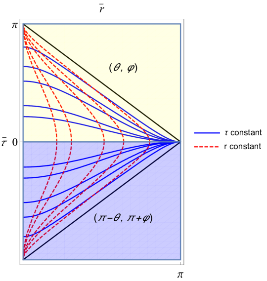
Figure 5: This picture is a conformal (Not Penrose) diagram, representing DQFT in (expanding) flat FLRW dS in terms of parametric time $\bar{\tau}$ and the compactified radial coordinate $\bar{r}$. The shaded quadrants, in yellow and blue, represents spatial regions related by parity, and where conformal time is positive in one region and negative in the other. A field operator in dS DQFT is represented by the direct sum of field operators populating the yellow and blue regions following (6.21).

Finally, we would like to comment a bit further on the significance of DQFT S-matrix definition in dS (6.36). As we can clearly verify, (6.36) is invariant under $\mathcal{P}\mathcal{T}$ ($\mathcal{C}\mathcal{P}\mathcal{T}$ in the context of charged fields) as far as the interaction Hamiltonian obeys the symmetry. Furthermore, we can now understand that the meaning of asymptotic states, that we define in SQFT, are slightly different in curved spacetime where the horizon effects must be seriously taken into account. However, it seems not an impossible task to make sense of QFTCS as it is expected from the most recent seminal papers by Giddings and Witten [8, 52]. We anticipate that our approach to QFTCS could contribute to further understand the subject. In the next section we will discuss, and propose views, about the implications of our study to the quantum gravity research field.

6.4.1 Comments about dS QFT in closed or global dS

As we discussed earlier, dS spacetime can be expressed in several coordinate frames due to its symmetries. When we express dS metric in a particular set of coordinates, we automatically fix our imaginary observer. In the previous section we have discussed dS in flat FLRW, which is the most relevant one for applications in the context of inflationary cosmology. However, closed dS metric (6.14) or its most often called the global dS spacetime [76] has been the popular subject of investigation from theoretical point of view [74]. The imaginary observer, in closed dS spacetime, experiences the Universe evolving from contraction to expansion, which we describe as a transition from the phase of growing to shrinking horizon $r_{H}$. This definition is independent of presumptions associated with cosmic time arrow (see Sec. 6.1). To implement direct-sum quantization we essentially need a notion of time reversal operation without changing the character of Universe (i.e., either expanding or contracting) which is given by (6.18). Such as in the flat FLRW dS case (6.21) we can analogously expand the scalar field operator as direct-sum of two components in closed dS, however the difference is that the (direct-sum) vaccum of closed dS would be different because the mode functions are also different. Physically, during contraction we will have the modes entering the horizon and during the expansion phase we will have the modes exiting the horizon, like in the flat FLRW dS case. Similar to flat FLRW, we can analogously have unitarity and observer complementarity in closed dS as well with direct-sum Fock space structure. Defining the scattering problem in closed dS is actually contextual because any scattering process can happen during , i) the contraction phase, ii) the expansion phase, iii) involving transition from contraction to expansion. S-matrix formulation in closed dS was addressed in the past [38] but such framework only discusses case (iii), with pre-scattering states in the contracting phase and post scattering states in the expanding phase. We note that this is a very particular scenario for a scattering problem. Generically, scattering can happen at any stage of Universe evolution, therefore, it is vital to study the cases (i), (ii) and (iii) very carefully. Having mentioned this, we indeed defer the detailed studies of closed dS to future investigations.

7 Possible implications of direct-sum QFTCS to quantum gravity

There are two points of view about dS within the quantum gravity research community. The first is to formulate a quantum gravity theory whose classical or semiclassical limit is dS [61, 87, 59]. This direction of research has been found to be an extremely arduous one, with a multitude of speculations taking a central spot due to the different possibilities one can have in the formulation of quantum gravity [69, 85, 88, 65, 89, 90]. Furthermore, the understanding of dS is most often dominated from the holography conjecture approach to quantum gravity [91, 74, 92, 93] where one sees the appearance of two asymptotic conformal field theories (CFTs) corresponding to the bulk description of gravity. This feature not only exist in the dS/CFT holographic proposals, but also in the AdS/CFT holographies where there are no horizons [58]. In different contexts, a quantum state in curved spacetime is formulated as an entangled state represented by tensor product of Hilbert spaces associated with the dual CFTs, or the so called thermo field double state in the holographic description of CFT [88, 69]. Although, the present work is not fully within the context of quantum gravity, we would like to propose that one can explore the DQFT formulation in the context of holographic version of quantum gravity without invoking any kind of entanglements between two classically disconnected worlds, or Universes, or two sided representations of spacetimes. We think DQFTCS might also be useful to make a new attempt to realize dS in string theory.

We would also would like to comment on the difference between DQFT in (expanding) FLRW flat dS and the elliptic view of dS, which is studied from the holographic point of view [30, 81]. First of all, elliptic dS is a proposal dating back to Schrödinger [29], which is based on the classical identification of two expanding branches of dS in the ellipsoid that is embedded in 5D Minkowski. In [30, 81] a S-matrix is proposed for dS, which is fully based on this classical connection of spacetime regions, through the antipodal identification. Such a framework becomes problematic once we have departure from dS spacetime, where the antipodal identification leads to closed time like curves [71]. In the DQFTCS approach we do not invoke any classical identification of spacetime, but rather construct a direct-sum Fock state which is explicitly $\mathcal{C}\mathcal{P}\mathcal{T}$  invariant and, further, consistent with observer complementarity. Therefore, this framework will have interesting implications to the program of quantum gravity in dS [62].

The second point of view about dS, within quantum gravity research, is the bottom up approach which is aimed to formulate a robust QFTCS before stepping into the fully unknown arena of quantum gravity. This is exactly the point of view taken in this paper. We would like to acknowledge several studies, that have explored stability of dS spacetime via quantum loop corrections due to matter fields [72, 94], have given us a way to build effective field theories (EFTs) of gravity for dS spacetime. We think our dS DQFT proposal will further shed light on building a correct QFTCS and, eventually, allow us to compute dS unitary scattering amplitudes, which can lead to interesting implications in the context of cosmological applications beyond current studies [95, 96, 97, 98].

8 Conclusions and Outlook

QFTCS constitutes an important field of study before we can step into form a consistent framework for quantum gravity. The main difficulty, for QFTCS (in the context of curved spacetimes with horizons), is due to the lack a globally definable concept of time. However, we must stress that this difficulty is expected and, in fact, this issue is why it is often said that GR and quantum mechanics are not compatible with each other. QFTCS is an inevitable obstacle that needs to be overcomed before tackling the unknown Planck scale physics, unification of fundamental forces or the issue of GR non-renormalizability. Evidently, we do not at all ignore several decades of developments in the field of quantum gravity [7]. Our intention is to highlight the unavoidable importance of QFTCS, which surely give us better foundations for bigger challenges such as quantum gravity. Let us emphasize that we are speaking about QFTCS in a totally semiclassical sense, i.e, just up to the KG field quantization in curved spacetime. We start by defining a physically reasonable vacuum, obtaining unitarity (in the sense that pure states should not evolve to mixed within the horizon) and ultimately making a right platform for the discussion of the S-matrix. Opposing popular beliefs, about the impossibility of constructing QFTCS with a S-matrix, we start with fundamental questions about the concept of time in quantum theory (where it has the status of just a parameter). We started our investigation by reviewing very meticulously textbook SQFT. We think it is possible to make several non-trivial observations regarding the way we perform quantization in Minkowski background, which actually follows from our conceived notion of time arrow. In the next step, we discussed the often ignored fact about $\mathcal{C}\mathcal{P}\mathcal{T}$  invariance of scattering amplitudes, in SQFT, which holds to any perturbative order (In Sydney Coleman own words found in p. 238 of [2]). This fact shows us how important discrete symmetries are in quantum theory and this might constitutes a good starting point to think about QFTCS. Furthermore, we certainly know about particles and anti-particles in nature, which are understood under the time reflection operation in SQFT. In addition, we clearly know the role of $\mathcal{C}\mathcal{P}\mathcal{T}$  theorem in SQFT, that tell us precisely what bosonic and fermionic states are. These previous examples are enough to convey the meaning of discrete symmetries in SQFT. Searching ways to accomodate these in curved spacetimes should play an important role to setup the foundations for QFTCS. Even if the fundamental description of nature is based on strings (not particles) near Planck scales, there is a huge energy difference between the standard model and Planck scales. Therefore, QFTCS is the first and foremost step before hitting full quantum gravity regime.

In this paper, we developed a direct-sum QFT for Minkowski spacetime and showed the explicit construction of $\mathcal{C}\mathcal{P}\mathcal{T}$  invariance, starting from quantization itself. DQFT approach opens a new door for the meaning of time in QFT and it is certainly useful to tackle the lack of global concept of time in curved spacetime. DQFT brings a new commutation relation for the operators defined in the direct-sum Fock space (4.27), which adds to the usual notion of causality found in QFT textbook formulation. We implement a construction for QFTCS, especially in the context of flat (expanding) FLRW dS spacetime. dS direct-sum QFT satisfies unitarity and observer complementarity. In agreement with (4.27), the commutation relation (6.26) emerges in our formulation of dS DQFT, making it compatible with the principle that operators corresponding to causally separated points should commute. Furthermore, we laid some foundational thoughts for defining the scattering problem (S-matrix) in dS. Our approach to QFTCS is not just theoretical, we also explored possible observational evidence for it, obtaining predictions for the hemispherical asymmetry of primordial power spectra derived in the context of inflation [23].

A future extension of our work would be to understand the quantization of fermions in curved spacetime and fully solve a scattering problem in DQFTCS. There is still a very long way for a definitive QFTCS and we expect that the subject further can motivate lots of conumdrums and surprising revelations. In a companion work, we are addressing another challenging spacetime in QFTCS which is Schwarzchild BH [51].

Our final remark is, quantum gravity research is actually both exciting and dangerous, the latter is mainly because there is an infinitely extendable room for speculations which often can potentially swamp us in the theoretical landscapes where it is indiscernible to decipher physical Universe that we observe. However, if we do carry the torch lights of unitarity and renormalizability we can definitely anchor quantum gravity research and reduce the plethora of uncertainties. QFTCS is an unavoidable barrier we need to cross first for unitarity and we sincerely hope our present investigation paves a way for interesting explorations in merging the quantum & gravity.

Appendix A Direct-sum Hilbert space construction of quantum mechanics

In Sec. 4 we have learned the direct-sum Fock space construction of QFT. Historically, QFT formulation has hailed with significant inputs from QM, therefore, it is natural to ask what direct-sum Fock space QFT could mean for QM. Here, we give a glimpse of it for completeness, deferring the detailed investigation to the future. It is worth to notice recent studies, both in the theoretical and experimental domains, about the time symmetric nature of quantum theory [99, 100, 44].

Let us start with Schrödinger equation (3.1) which we label as Schrödinger equation I that gives the time evolution of state $|\psi_{I}\rangle_{t}=e^{-iEt}|\psi_{I}\rangle_{0}$ according to

$$i\frac{\partial|\psi_{I}\rangle}{\partial t}=\hat{H}|\psi_{I}\rangle$$ (A.1)

where $\hat{H}$ is the Hamiltonian, whose precise form is irrelevant for the present discussion. However, we assume it to be $\mathcal{P}\mathcal{T}$ symmetric as many physical systems (without involving gravity) in nature are

$$[\hat{H},\,\mathcal{P}\mathcal{T}]=0\,.$$ (A.2)

Because of the fact that (A.2) holds well in many instances, there is a whole field of research on $\mathcal{P}\mathcal{T}$ symmetric formulations of QM (See [101] for more details). However, our framework does not fall into the so-called $\mathcal{P}\mathcal{T}$ symmetric QM of [101].

Let us now take the unconventional form of Schrödinger equation (3.2), naming it as Schrödinger equation II, which is

$$-i\frac{\partial|\psi_{II}\rangle}{\partial t}=\hat{H}|\psi_{II}\rangle$$ (A.3)

The state vector, according to (A.3), evolves as $|\psi_{II}\rangle_{t}=e^{iEt}|\psi_{II}\rangle_{0}$ and it is the positive energy state. Comparing (A.1) and (A.3), we can take states $|\psi_{I}\rangle,\,\,|\psi_{II}\rangle$ as evolving forward and backward in time respectively.

Here, we attempt to make a new formulation of QM that is inbuild with $\mathcal{P}\mathcal{T}$ symmetry. Recalling again that time is a parameter in quantum theory,

We divide position space into two parts, I and II, based on the parity operation $\mathcal{P}$. Subsequently, we assign time evolution, for states in spatial regions I and II, according to Schrödinger equation I (A.1) and II (A.3) respectively. Finally we construct a single particle quantum mechanical state, in the whole position space, using the direct-sum of states in region I and II. Thus, the total Hilbert space $\mathcal{H}$ of single particle state becomes the direct-sum of the Hilbert spaces corresponding to the region I and II, respectively.

Therefore, in the direct-sum Hilbert space construction of QM, the single particle quantum state is

$$|\psi\rangle=\frac{|\psi_{I}\rangle\oplus|\psi_{II}\rangle}{\sqrt{2}}=\frac{1}{\sqrt{2}}\begin{pmatrix}|\psi_{I}\rangle&\\ |\psi_{II}\rangle\end{pmatrix}\,.$$ (A.4)

The factor of $\sqrt{2}$ in (A.4) is a normalization to have the total probabilities add up to 1 as

$$\langle\psi|\psi\rangle=\frac{\langle\psi_{I}|\psi_{I}\rangle}{2}+\frac{\langle\psi_{II}|\psi_{II}\rangle}{2}=1\,.$$ (A.5)

This clearly shows the concept of direct-sum, which is totally different from the usual summation, which indicate superposition of states in quantum theory. In (A.4), state vector $|\psi\rangle$ is defined in a Hilbert space which can be written as

$$\mathcal{H}=\mathcal{H}_{I}\oplus\mathcal{H}_{II}\,,$$ (A.6)

where $\mathcal{H}_{I}$ and $\mathcal{H}_{II}$ are the Hilbert space corresponding to the spatial region I and II, which are parity conjugates of each other. In region I, quantum mechanics is governed by (A.1), in which the canonical commutation relation between position and momentum of a single particle is given by

$$[\hat{x}_{1},\,\hat{p}_{1}]=i\hbar\,,$$ (A.7)

whereas, in region II, position and momentum uncertainty is dictated by

$$[\hat{x}_{2},\,\hat{p}_{2}]=-i\hbar\,,$$ (A.8)

where the change of $i\to-i$ is a consequence of the time reversal operation. Following (A.6), the operators (say $\hat{\mathcal{O}}$) that act on the state vectors in the total Hilbert space become the direct-sum of the operators corresponding to $\mathcal{H}_{I}$ and $\mathcal{H}_{II}$ as

$$\hat{\mathcal{O}}=\hat{\mathcal{O}}_{I}\oplus\hat{\mathcal{O}}_{II}=\begin{pmatrix}\hat{\mathcal{O}}_{I}&0\\ 0&\hat{\mathcal{O}}_{II}\end{pmatrix}$$ (A.9)

As we see in (A.9) the direct-sum of operators mean extending the matrix operators into block diagonal form which act on the higher dimensional state vectors $|\psi\rangle$ as written in (A.4). From (A.9), we deduce that states belonging to the direct-sum Hilbert space, evolve according to the following equation which we call as direct-sum Schrödinger equation

$$i\frac{\partial}{\partial t}\begin{pmatrix}|\psi_{I}\rangle&\\ |\psi_{II}\rangle\end{pmatrix}=\begin{pmatrix}\hat{H}&0\\ 0&-\hat{H}\end{pmatrix}\begin{pmatrix}|\psi_{I}\rangle&\\ |\psi_{II}\rangle\end{pmatrix}\,,$$ (A.10)

which is simply the direct-sum of the Schödinger equations I (A.1) and II (A.3), respectively. It is worth to note that (A.4) is explicitly $\mathcal{P}\mathcal{T}$ symmetric, because the direct-sum state vector $|\psi\rangle$ is $\mathcal{P}\mathcal{T}$ invariant. For physical systems, whose Hamilitonians are $\mathcal{P}\mathcal{T}$ symmetric, the formulation of standard Schrödinger equation (3.1) would not yield $\mathcal{P}\mathcal{T}$ symmetric states but direct-sum Schrödinger equation does yield $\mathcal{P}\mathcal{T}$ symmetric states. Nevertheless, if we restrict to $\mathcal{P}\mathcal{T}$ symmetric physical systems we cannot see any difference between results of standard Schrödinger equation (3.1) and the direct-sum Schrödinger equation. However, in the context of physical systems whose Hamiltonian breaks the $\mathcal{P}\mathcal{T}$ symmetry (but remain Hermitian) one might see differences in results, which is for the moment beyond the scope of the current investigation.

References

- [1] R. M. Wald, General Relativity. Chicago Univ. Pr., Chicago, USA, 1984.
- [2] S. Coleman, Lectures of Sidney Coleman on Quantum Field Theory. WSP, Hackensack, 12, 2018.
- [3] B. W. Roberts, “Reversing the Arrow of Time,” arXiv:2212.03489 [physics.hist-ph].
- [4] LIGO Scientific, Virgo Collaboration, B. P. Abbott et al., “Observation of Gravitational Waves from a Binary Black Hole Merger,” Phys. Rev. Lett. 116 no. 6, (2016) 061102, arXiv:1602.03837 [gr-qc].
- [5] Event Horizon Telescope Collaboration, K. Akiyama et al., “First Sagittarius A* Event Horizon Telescope Results. I. The Shadow of the Supermassive Black Hole in the Center of the Milky Way,” Astrophys. J. Lett. 930 no. 2, (2022) L12.
- [6] M. Rummel and C. P. Burgess, “Constraining Fundamental Physics with the Event Horizon Telescope,” JCAP 05 (2020) 051, arXiv:2001.00041 [gr-qc].
- [7] L. Buoninfante and K. S. Kumar, “Quantum gravity, higher derivatives and nonlocality,” Nuovo Cim. C 45 no. 2, (2022) 25.
- [8] S. B. Giddings, “The deepest problem: some perspectives on quantum gravity,” arXiv:2202.08292 [hep-th].
- [9] S. B. Giddings, “Comparing models for a unitary black hole S-matrix,” arXiv:2212.14551 [hep-th].
- [10] M. Visser, “Gravitational vacuum polarization,” in 8th Marcel Grossmann Meeting on Recent Developments in Theoretical and Experimental General Relativity, Gravitation and Relativistic Field Theories (MG 8), pp. 842–844. 6, 1997. arXiv:gr-qc/9710034.
- [11] S. D. Mathur, “The Information paradox: A Pedagogical introduction,” Class. Quant. Grav. 26 (2009) 224001, arXiv:0909.1038 [hep-th].
- [12] X. Calmet and S. D. H. Hsu, “A brief history of Hawking’s information paradox,” EPL 139 no. 4, (2022) 49001, arXiv:2207.08671 [hep-th].
- [13] A. Almheiri, D. Marolf, J. Polchinski, and J. Sully, “Black Holes: Complementarity or Firewalls?,” JHEP 02 (2013) 062, arXiv:1207.3123 [hep-th].
- [14] B. Allen, “Vacuum states in de sitter space,” Phys. Rev. D 32 (Dec, 1985) 3136–3149. https://link.aps.org/doi/10.1103/PhysRevD.32.3136.
- [15] C. Kiefer, D. Polarski, and A. A. Starobinsky, “Quantum to classical transition for fluctuations in the early universe,” Int. J. Mod. Phys. D 7 (1998) 455–462, arXiv:gr-qc/9802003.
- [16] R. Bousso, “Cosmology and the S-matrix,” Phys. Rev. D 71 (2005) 064024, arXiv:hep-th/0412197.
- [17] C. Kiefer and D. Polarski, “Why do cosmological perturbations look classical to us?,” Adv. Sci. Lett. 2 (2009) 164–173, arXiv:0810.0087 [astro-ph].
- [18] A. Perez, H. Sahlmann, and D. Sudarsky, “On the quantum origin of the seeds of cosmic structure,” Class. Quant. Grav. 23 (2006) 2317–2354, arXiv:gr-qc/0508100.
- [19] D. Sudarsky, “Shortcomings in the Understanding of Why Cosmological Perturbations Look Classical,” Int. J. Mod. Phys. D 20 (2011) 509–552, arXiv:0906.0315 [gr-qc].
- [20] J. B. Hartle, The Quantum Mechanical Arrows of Time, pp. 113–128. 2014. arXiv:1301.2844 [quant-ph].
- [21] J. B. Hartle, “Arrows of Time and Initial and Final Conditions in the Quantum Mechanics of Closed Systems Like the Universe,” arXiv:2002.07093 [gr-qc].
- [22] N. E. Mavromatos, “On CPT symmetry: Cosmological, quantum gravitational and other possible violations and their phenomenology,” Springer Proc. Phys. 92 (2004) 43–72, arXiv:hep-ph/0309221.
- [23] K. S. Kumar and J. Marto, “Hemispherical asymmetry of primordial power spectra,” arXiv:2209.03928 [gr-qc].
- [24] G. ’t Hooft, “Time, the Arrow of Time, and Quantum Mechanics,” Front. in Phys. 6 (2018) 81, arXiv:1804.01383 [quant-ph].
- [25] G. ’t Hooft, “Deterministic Quantum Mechanics: The Mathematical Equations,” Front. in Phys. 8 (2020) 253, arXiv:2005.06374 [quant-ph].
- [26] N. D. Birrell and P. C. W. Davies, Quantum Fields in Curved Space. Cambridge Monographs on Mathematical Physics. Cambridge Univ. Press, Cambridge, UK, 2, 1984.
- [27] S. Hollands and R. M. Wald, “Axiomatic quantum field theory in curved spacetime,” Commun. Math. Phys. 293 (2010) 85–125, arXiv:0803.2003 [gr-qc].
- [28] S. Hollands and R. M. Wald, “Quantum fields in curved spacetime,” Phys. Rept. 574 (2015) 1–35, arXiv:1401.2026 [gr-qc].
- [29] Erwin Schrodinger, Expanding universes. 1956.
- [30] M. Parikh, I. Savonije, and E. Verlinde, “Elliptic de sitter space:ds/z2,” Physical Review D 67 no. 6, (Mar, 2003) . http://dx.doi.org/10.1103/PhysRevD.67.064005.
- [31] V. Mukhanov and S. Winitzki, Introduction to quantum effects in gravity. Cambridge University Press, 6, 2007.
- [32] J. S. Ben-Benjamin et al., “Unruh Acceleration Radiation Revisited,” Int. J. Mod. Phys. A 34 no. 28, (2019) 1941005, arXiv:1906.01729 [quant-ph].
- [33] L. C. B. Crispino, A. Higuchi, and G. E. A. Matsas, “The Unruh effect and its applications,” Rev. Mod. Phys. 80 (2008) 787–838, arXiv:0710.5373 [gr-qc].
- [34] L. H. Ford, “Quantum field theory in curved space-time,” in 9th Jorge Andre Swieca Summer School: Particles and Fields, pp. 345–388. 7, 1997. arXiv:gr-qc/9707062.
- [35] R. M. Wald, Quantum Field Theory in Curved Space-Time and Black Hole Thermodynamics. Chicago Lectures in Physics. University of Chicago Press, Chicago, IL, 1995.
- [36] T. Lancaster and S. J. Blundell, Quantum Field Theory for the Gifted Amateur. Oxford University Press, 2014.
- [37] M. E. Peskin and D. V. Schroeder, An Introduction to quantum field theory. Addison-Wesley, Reading, USA, 1995.
- [38] M. Srednicki, Quantum field theory. Cambridge University Press, 1, 2007.
- [39] L. H. Ryder, QUANTUM FIELD THEORY. Cambridge University Press, 6, 1996.
- [40] J. F. Donoghue and G. Menezes, “Arrow of Causality and Quantum Gravity,” Phys. Rev. Lett. 123 no. 17, (2019) 171601, arXiv:1908.04170 [hep-th].
- [41] J. F. Donoghue and G. Menezes, “Quantum causality and the arrows of time and thermodynamics,” Prog. Part. Nucl. Phys. 115 (2020) 103812, arXiv:2003.09047 [quant-ph].
- [42] J. F. Donoghue and G. Menezes, “Causality and gravity,” JHEP 11 (2021) 010, arXiv:2106.05912 [hep-th].
- [43] J. B. Conway, A course in functional analysis / John B. Conway. Graduate texts in mathematics ; 96. Springer Science+Business Media, New York, 2nd ed. ed., 2010.
- [44] N. L. Harshman, “Symmetry, Structure, and Emergent Subsystems,” arXiv e-prints (Jan., 2018) arXiv:1801.08755, arXiv:1801.08755 [quant-ph].
- [45] E. A. Mazenc and D. Ranard, “Target space entanglement entropy,” JHEP 03 (2023) 111, arXiv:1910.07449 [hep-th].
- [46] G. C. Wick, A. S. Wightman, and E. P. Wigner, “The intrinsic parity of elementary particles,” Phys. Rev. 88 (1952) 101–105.
- [47] nLab authors, “superselection theory.” https://ncatlab.org/nlab/show/superselection+theory, June, 2023. Revision 10.
- [48] D. Giulini, “Superselection Rules,” arXiv:0710.1516 [quant-ph].
- [49] J. B. Griffiths and J. Podolsky, Exact Space-Times in Einstein’s General Relativity. Cambridge Monographs on Mathematical Physics. Cambridge University Press, Cambridge, 2009.
- [50] D. Harlow, “Jerusalem Lectures on Black Holes and Quantum Information,” Rev. Mod. Phys. 88 (2016) 015002, arXiv:1409.1231 [hep-th].
- [51] K. S. Kumar and J. Marto, “Towards Unitary Quantum Field Thoery in Curved Spacetime II: The case of Schwarzchild Blackhole,” arXiv:2305.XXXX [gr-qc].
- [52] E. Witten, “Why Does Quantum Field Theory In Curved Spacetime Make Sense? And What Happens To The Algebra of Observables In The Thermodynamic Limit?,” arXiv:2112.11614 [hep-th].
- [53] L. Susskind, “A Paradox and its Resolution Illustrate Principles of de Sitter Holography,” arXiv:2304.00589 [hep-th].
- [54] V. Chandrasekaran, R. Longo, G. Penington, and E. Witten, “An algebra of observables for de Sitter space,” JHEP 02 (2023) 082, arXiv:2206.10780 [hep-th].
- [55] J. Hartong, “On problems in de Sitter spacetime physics: scalar fields, black holes and stability,” Master’s thesis, Groningen U., 2004.
- [56] J. Polchinski, “S matrices from AdS space-time,” arXiv:hep-th/9901076.
- [57] A. L. Fitzpatrick and J. Kaplan, “Unitarity and the Holographic S-Matrix,” JHEP 10 (2012) 032, arXiv:1112.4845 [hep-th].
- [58] L. Freidel, “Reconstructing AdS/CFT,” arXiv:0804.0632 [hep-th].
- [59] V. Balasubramanian, P. Horava, and D. Minic, “Deconstructing de Sitter,” JHEP 05 (2001) 043, arXiv:hep-th/0103171.
- [60] L. Aalsma, A. Cole, E. Morvan, J. P. van der Schaar, and G. Shiu, “Shocks and information exchange in de Sitter space,” JHEP 10 (2021) 104, arXiv:2105.12737 [hep-th].
- [61] L. Susskind, “De Sitter Holography: Fluctuations, Anomalous Symmetry, and Wormholes,” Universe 7 no. 12, (2021) 464, arXiv:2106.03964 [hep-th].
- [62] E. Witten, “Quantum gravity in de Sitter space,” in Strings 2001: International Conference. 6, 2001. arXiv:hep-th/0106109.
- [63] A. A. Starobinsky, “A New Type of Isotropic Cosmological Models Without Singularity,” Phys. Lett. B91 (1980) 99–102.
- [64] V. Balasubramanian, A. Kar, and T. Ugajin, “Islands in de Sitter space,” JHEP 02 (2021) 072, arXiv:2008.05275 [hep-th].
- [65] V. Balasubramanian, A. Kar, and T. Ugajin, “Entanglement between two gravitating universes,” Class. Quant. Grav. 39 no. 17, (2022) 174001, arXiv:2104.13383 [hep-th].
- [66] D. Anninos, “De Sitter Musings,” Int. J. Mod. Phys. A 27 (2012) 1230013, arXiv:1205.3855 [hep-th].
- [67] N. Goheer, M. Kleban, and L. Susskind, “The Trouble with de Sitter space,” JHEP 07 (2003) 056, arXiv:hep-th/0212209.
- [68] M. Spradlin, A. Strominger, and A. Volovich, “Les Houches lectures on de Sitter space,” in Les Houches Summer School: Session 76: Euro Summer School on Unity of Fundamental Physics: Gravity, Gauge Theory and Strings, pp. 423–453. 10, 2001. arXiv:hep-th/0110007.
- [69] T. Hartman, Y. Jiang, and E. Shaghoulian, “Islands in cosmology,” JHEP 11 (2020) 111, arXiv:2008.01022 [hep-th].
- [70] N. Sánchez, “Quantum field theory and the “elliptic interpretation” of de sitter spacetime,” Nuclear Physics B 294 (1987) 1111–1137. https://www.sciencedirect.com/science/article/pii/0550321387906250.
- [71] A. Aguirre and S. Gratton, “Inflation without a beginning: A null boundary proposal,” Physical Review D 67 no. 8, (Apr, 2003) . http://dx.doi.org/10.1103/PhysRevD.67.083515.
- [72] E. T. Akhmedov, “Lecture notes on interacting quantum fields in de Sitter space,” Int. J. Mod. Phys. D 23 (2014) 1430001, arXiv:1309.2557 [hep-th].
- [73] A. Riotto, “Inflation and the theory of cosmological perturbations,” ICTP Lect. Notes Ser. 14 (2003) 317–413, arXiv:hep-ph/0210162.
- [74] R. Bousso, “Adventures in de Sitter space,” in Workshop on Conference on the Future of Theoretical Physics and Cosmology in Honor of Steven Hawking’s 60th Birthday, pp. 539–569. 5, 2002. arXiv:hep-th/0205177.
- [75] Y.-b. Kim, C. Y. Oh, and N. Park, “Classical geometry of de Sitter space-time: An Introductory review,” arXiv:hep-th/0212326.
- [76] T. Hartman, “Lecture Notes on Classical de Sitter Space,” (2017) .
- [77] V. Mukhanov, Physical Foundations of Cosmology. Cambridge University Press, Oxford, 2005.
- [78] C. Rovelli, “Notes for a brief history of quantum gravity,” in Recent developments in theoretical and experimental general relativity, gravitation and relativistic field theories. Proceedings, 9th Marcel Grossmann Meeting, MG’9, Rome, Italy, July 2-8, 2000. Pts. A-C, pp. 742–768. 2000. arXiv:gr-qc/0006061 [gr-qc].
- [79] C. Rovelli, Quantum gravity. Cambridge Monographs on Mathematical Physics. Univ. Pr., Cambridge, UK, 2004.
- [80] G. W. Gibbons and S. W. Hawking, “Cosmological Event Horizons, Thermodynamics, and Particle Creation,” Phys. Rev. D 15 (1977) 2738–2751.
- [81] M. Parikh and E. Verlinde, “De sitter holography with a finite number of states,” Journal of High Energy Physics 2005 no. 01, (Feb, 2005) 054–054. http://dx.doi.org/10.1088/1126-6708/2005/01/054.
- [82] L. Dyson, J. Lindesay, and L. Susskind, “Is there really a de Sitter/CFT duality?,” JHEP 08 (2002) 045, arXiv:hep-th/0202163.
- [83] L. Susskind, L. Thorlacius, and J. Uglum, “The Stretched horizon and black hole complementarity,” Phys. Rev. D 48 (1993) 3743–3761, arXiv:hep-th/9306069.
- [84] G. ’t Hooft, “On the Quantum Structure of a Black Hole,” Nucl. Phys. B 256 (1985) 727–745.
- [85] E. Shaghoulian, “The central dogma and cosmological horizons,” JHEP 01 (2022) 132, arXiv:2110.13210 [hep-th].
- [86] X. Gao, “Primordial Non-Gaussianities of General Multiple Field Inflation,” JCAP 0806 (2008) 029, arXiv:0804.1055 [astro-ph].
- [87] L. Aalsma and G. Shiu, “Chaos and complementarity in de Sitter space,” JHEP 05 (2020) 152, arXiv:2002.01326 [hep-th].
- [88] E. Shaghoulian and L. Susskind, “Entanglement in De Sitter space,” JHEP 08 (2022) 198, arXiv:2201.03603 [hep-th].
- [89] T. Chakraborty, J. Chakravarty, V. Godet, P. Paul, and S. Raju, “The Hilbert space of de Sitter quantum gravity,” arXiv:2303.16315 [hep-th].
- [90] G. Maniccia, G. Montani, and S. Antonini, “QFT in curved spacetime from quantum gravity: Proper WKB decomposition of the gravitational component,” Phys. Rev. D 107 no. 6, (2023) L061901, arXiv:2302.10832 [gr-qc].
- [91] A. Strominger, “The dS / CFT correspondence,” JHEP 10 (2001) 034, arXiv:hep-th/0106113.
- [92] M. Fabinger and E. Silverstein, “D-Sitter space: Causal structure, thermodynamics, and entropy,” JHEP 12 (2004) 061, arXiv:hep-th/0304220.
- [93] H. Geng, “Non-local entanglement and fast scrambling in de-Sitter holography,” Annals Phys. 426 (2021) 168402, arXiv:2005.00021 [hep-th].
- [94] D. Green, “EFT for de Sitter Space,” arXiv:2210.05820 [hep-th].
- [95] R. Ferrero and C. Ripken, “De Sitter scattering amplitudes in the Born approximation,” SciPost Phys. 13 (2022) 106, arXiv:2112.03766 [hep-th].
- [96] R. Ferrero and C. Ripken, “Quadratic gravity scattering amplitudes in de Sitter spacetime,” arXiv:2212.08052 [hep-th].
- [97] N. Arkani-Hamed and J. Maldacena, “Cosmological Collider Physics,” arXiv:1503.08043 [hep-th].
- [98] D. Baumann, D. Green, A. Joyce, E. Pajer, G. L. Pimentel, C. Sleight, and M. Taronna, “Snowmass White Paper: The Cosmological Bootstrap,” in Snowmass 2021. 3, 2022. arXiv:2203.08121 [hep-th].
- [99] D. Geiger and Z. M. Kedem, “A theory for the time arrow,” 2019.
- [100] T. Strömberg, P. Schiansky, M. T. Quintino, M. Antesberger, L. Rozema, I. Agresti, v. Brukner, and P. Walther, “Experimental superposition of time directions,” arXiv:2211.01283 [quant-ph].
- [101] C. M. Bender, “Introduction to PT-Symmetric Quantum Theory,” Contemp. Phys. 46 (2005) 277–292, arXiv:quant-ph/0501052.