On the Time-Varying Structure of the Arbitrage Pricing Theory using the Japanese Sector Indices

Abstract: This paper is the first study to examine the time instability of the APT in the Japanese stock market. In particular, we measure how changes in each risk factor affect the stock risk premiums to investigate the validity of the APT over time, applying the rolling window method to Fama and MacBeth’s (1973) two-step regression and Kamstra and Shi’s (2023) generalized GRS test. We summarize our empirical results as follows: (1) the APT is supported over the entire sample period but not at all times, (2) the changes in monetary policy greatly affect the validity of the APT in Japan, and (3) the time-varying estimates of the risk premiums for each factor are also unstable over time, and they are affected by the business cycle and economic crises. Therefore, we conclude that the validity of the APT as an appropriate model to explain the Japanese sector index is not stable over time.

Keywords: Time-Varying Coefficient; Arbitrage Pricing Theory; Monetary Policy; Macroeconomic Risk; Generalized GRS Test

JEL Classification Numbers: G12; G14; E52.

1 Introduction

Economists have been investigating which asset pricing model is appropriate for explaining the behavior of the stock returns since Sharpe (1964) and Lintner (1965) proposed the capital asset pricing model (CAPM). As a result, there are a large number of models to explain the stock returns. Among them, the intertemporal CAPM of Merton (1973), the arbitrage pricing theory (APT) of Ross (1976), and Fama and French’s (1993; 2015; 2016) multi-factor models (FF models) are often investigated in previous studies. We can interpret the FF models as models that aim to capture the market anomalies such as the size-risk factor and the value-risk factor. However, some previous studies show that the market efficiency or the predictability of stock returns change over time, and they are affected by the various exogenous shocks (see Kim et al. (2011), Ito et al. (2016), and Noda (2016)). In other words, the FF models may not sufficiently explain the stock returns because they do not capture the exogenous shocks. Then, we apply the APT to explain the stock returns because the APT can explicitly consider the exogenous shocks and capture the impact of them on the stock returns.

Many previous studies examine the validity of the APT in the U.S. stock market since Chen et al. (1986). On the other hand, there are not so many previous studies that test the APT in the Japanese stock market. Hamao (1988) is the first study to test the APT as an appropriate pricing model in the Japanese stock market from 1975 to 1984 using monthly data. He concludes that the APT is valid in explaining the stock returns in Japan. Azeez and Yonezawa (2006) explore whether the validity of the APT changes by splitting the sample periods into the following three periods: the pre-bubble, bubble, and post-bubble periods, focusing on the risk premium of real estate in the late 1980s using monthly data from January 1989 to December 1998. They show that the APT is supported regardless of the sample period, but real estate is not useful in explaining the returns on the Japanese stock market in any period. Tsuji (2007) examines whether risk premiums of other macroeconomic factors (e.g., money supply and gold), which are not considered in previous studies, are incorporated into the returns of Japanese sector indices using monthly data from February 1986 to December 2003. His empirical results show that the risk factors used in previous studies, except for crude oil and exchange rate related-factors, can explain the returns on the Japanese stock market. In addition, they find that the money supply, the gold prices, and the foreign exchange reserves help explain the returns on the Japanese stock market. On the other hand, they conclude that the other factors do not contribute much to explaining Japanese stock market returns.

In addition, we also introduce some related studies that focus on the impact of macroeconomic factors on the Japanese stock market. Kaneko and Lee (1995) examine the effectiveness of economic state variables, used in Chen et al. (1986) and Hamao (1988), in the U.S. and Japanese stock markets based on the vector autoregressive model during the period from January 1975 to December 1993. Their empirical results are not consistent with Hamao (1988), but are consistent with Chen et al. (1986). He and Ng (1998) examine whether the stock returns of Japanese multinationals are affected by changes in the exchange rate using monthly data from January 1979 to December 1993. They find that the depreciation (appreciation) of the yen has a positive (negative) effect on the stock returns of Japanese multinationals. Doukas et al. (1999) show that the risk premium on the foreign exchange is a significant component for explaining the Japanese sector indices using monthly data from January 1975 to December 1995. Moreover, they find that the risk premium changes over time in response to market conditions. Homma et al. (2005) examine whether investors carefully monitor the export intensity and net external position of Japanese firms and whether they are adequately reflected in stock prices based on a multifactor model that includes macroeconomic factors using daily data from January 5, 1983 to March 29, 1996. They find that stock investors carefully evaluate the export intensity and net external position of Japanese firms. Thorbecke (2020) estimates the sensitivity of risk factors in a multifactor model using daily returns on Japanese sector indices from January 6, 2020, to May 29, 2020. He finds that there is an asymmetry in sensitivity across sectors since the World Health Organization (WHO) declared the COVID-19 global pandemic.

However, there exist two empirical problems with the previous studies for the Japanese stock market. First, the previous studies use monthly data, except for Homma et al. (2005) and Thorbecke (2020). We believe that the stock returns are likely to be affected by the production activities of domestic firms and monetary policy. Therefore, the industrial production index and the money supply are often used as proxy variables but these variables do not have more high frequent data than monthly, so we cannot ensure a sufficient sample size. Second, the sample periods used in the previous study are too restrictive to examine the long-term validity of the APT. In particular, the sample periods of the sub-samples used in Azeez and Yonezawa (2006) is less than 100 months, which makes the results skeptical. In addition, Thorbecke (2020) examines the impact of the COVID-19 global pandemic on Japanese industries, but the sample period, from January 1 to May 29, 2020, is quite restrictive. Thus, it is difficult to say that we have elucidated the long-term impact of the COVID-19 global pandemic on the Japanese stock market.

Moreover, the previous studies argue that the APT is supported in the Japanese stock market, but the significance and sign condition of the estimates of risk premiums are quite different. We believe that the reason for this inconsistency in the empirical results of the previous studies is that they do not consider the time-varying structure of the APT. In other words, they implicitly assume that the stock market is stable over time. However, some previous studies, such as Kim et al. (2011), Ito et al. (2016), and Noda (2016), find that market efficiency (or stock predictability) varies over time because the environment surrounding the stock market keeps changing due to exogenous shocks such as economic crises. Therefore, we need to consider the time-varying structure of the APT. We then examine the time instability of the validity of the APT over time in the Japanese stock markets. In practice, we apply the rolling window method to Fama and MacBeth’s (1973) two-step regression using long-term daily data to verify the implicit assumption in previous studies that the market structure is stable over time. Finally, we perform the generalized Gibbons et al.’s (1989) test developed by Kamstra and Shi (2023) with the rolling window method to examine the validity of the APT over time.

The rest of this paper is organized as follows. Section 2 presents our methodology. Section 3 describes the data used in this paper. Section 4 shows our empirical results. Section 5 concludes this study.

2 Methodology

This section presents an empirical framework to examine the time instability of Ross’s (1976) APT using the Japanese sector indices.

2.1 Preliminaries

In the literature of modern finance, it is well known that the CAPM proposed by Sharpe (1964) and Lintner (1965) is the most basic framework to explain stock returns. However, the theoretical assumptions to hold the CAPM are quite strong and unrealistic, as shown in Ross (1976). In addition, Roll (1977) also criticizes that in most empirical studies on the CAPM, the market portfolio is limited to stocks (e.g., the Standard & Poor’s 500 and the Tokyo Stock Price Index) and does not include other financial assets.

Ross (1976) proposes the APT to address the theoretical and empirical problems of the CAPM discussed above. We can interpret the ATP as a theoretically relaxed model that explicitly considers how systematic risks such as business cycle, exchange rates, and policy changes, which cannot be eliminated under the CAPM, affect the returns on financial assets. The APT assumes that each investor (homogeneously) believes that the excess returns on the sector indices follow the $m$-factor generating model below:

$$r_{i,t}-r_{f,t}=\alpha_{i}+\sum_{j=1}^{m}\beta_{ij}f_{j,t}+\varepsilon_{i,t},\ \ i=1,\ldots,n,\ \ j=1,\ldots,m,\ \ m<n,\ \ t=1,\ldots,T,$$ (1)

where $r_{i,t}$ is the stock returns for each sector at time $t$, $r_{f,t}$ is the risk-free rate at time $t$, $\alpha_{i}$ is the constant term for each sector, $\beta_{ij}$ is the sensitivity to the $j$-th factor for each sector, $f_{j,t}$ is the $j$-th factor, which is a systematic risk affecting the risk premium for all sector indices at time $t$, and $\varepsilon_{i,t}$ is the error term specific to $i$-th sector at time $t$. We also make the following assumptions:

$${\mathbb{E}}[f_{j,t}]=0,\ \ {\mathbb{E}}[\varepsilon_{i,t}]=0,\ \ \mathbb{C}{\rm{ov}}(\varepsilon_{i,t},\varepsilon_{j,t})=0,\ \ \forall i\neq j.$$

Suppose that we now invest $x_{i}$ in any $i$-th sector. We can get $x_{i}$ for free if short selling is allowed. Specifically, we can construct a portfolio at no cost by investing all the funds if we borrow shares from a brokerage firm to short and sell them. The above constraints can be expressed as follows:

$$\sum_{i=1}^{n}x_{i}=0$$ (2)

Then, we construct a portfolio with no systematic risk $f_{j}$, i.e., it satisfies the condition in Equation (1). Since the sensitivity of the systematic risk $\beta_{ij}$ is assumed to be non-zero, the following orthogonal condition is satisfied for $x_{i}$.

$$\sum_{i=1}^{n}\sum_{j=1}^{m}x_{i}\beta_{ij}=0$$ (3)

Assuming that we can diversify away the unsystematic risk, any portfolio can be written as follows:

$$\sum_{i=1}^{n}x_{i}(r_{i,t}-r_{f,t}) = \sum_{i=1}^{n}x_{i}\alpha_{i}+\sum_{i=1}^{n}\sum_{i=1}^{m}x_{i}\beta_{ij}f_{j,t}+\sum_{i=1}^{n}x_{i}\varepsilon_{i,t}$$ (4)

$$\simeq \sum_{i=1}^{n}x_{i}\alpha_{i}+\sum_{i=1}^{n}\sum_{i=1}^{m}x_{i}\beta_{ij}f_{j,t}$$

$$= \sum_{i=1}^{n}x_{i}\alpha_{i}$$

Therefore, depending on the combination of $x_{i}$, it is possible to choose a portfolio with neither systematic nor unsystematic risk. We can understand that all portfolios satisfying the above conditions have no excess returns on average if there are no arbitrage opportunities. That is, if Equations (2) and (3) are satisfied, then the following equation is also necessarily satisfied.

$$\sum_{i=1}^{n}x_{i}(r_{i,t}-r_{f,t})=0\Leftrightarrow\sum_{i=1}^{n}x_{i}{\mathbb{E}}[r_{i,t}]-\sum_{i=1}^{n}x_{i}r_{f,t}=0\Leftrightarrow\sum_{i=1}^{n}x_{i}{\mathbb{E}}[r_{i,t}]=0,$$ (5)

where ${\mathbb{E}}[r_{i,t}]$ can be expressed as a linear combination of 1 and $\beta_{ij}$. In other words, there exist $m+1$ weights, $\lambda_{0},\lambda_{1},\ldots,\lambda_{m}$ such that

$${\mathbb{E}}[r_{i,t}]=\lambda_{0}+\sum_{j=1}^{m}\beta_{ij}\lambda_{j},\ \ i=1,...,n.$$ (6)

Now, we construct a portfolio consisting only of a risk-free asset, we obtain $r_{f}=\lambda_{0}$ ($\beta_{i,j}=0$). Hence Equation (6) can be rewritten as follows:

$${\mathbb{E}}[r_{i,t}]-r_{f}=\sum_{j=1}^{m}\beta_{ij}\lambda_{j},\ \ i=1,...,n,$$ (7)

The left-hand side of Equation (7) is the risk premium for the $i$-th sector. If the left-hand side is a risk premium, then the right-hand side must also be an expression of the risk premium. Therefore, $\lambda_{j}$ can be interpreted as the risk premium for the factor $j\ (j=1,...,m)$.

2.2 Fama and MacBeth’s (1973) Two-Step Regression with Rolling Windows

In this study, we employ Fama and MacBeth’s (1973) two-step regression with rolling windows as an empirical framework to examine the instability of the APT over time. In particular, we first regress risk premiums against systematic risks to estimate the sensitivity of each risk premium based on Equation (1). Then we also regress the mean of the risk premium against the estimated sensitivity to estimate the risk premium for each factor based on Equation (7). In the two-step regression, we employ the feasible generalized least squares (FGLS) estimator instead of the ordinary least squares (OLS) estimator used in many previous studies. This is because the estimation errors are said to be significant when we use the OLS estimator as shown in Shanken (1992).

Equation (1) can be written in the following matrix form:

$${\mbox{\boldmath$R$}}_{i}^{e}=\alpha_{i}+{\mbox{\boldmath$F$}}{\mbox{\boldmath$\beta$}}_{i}+{\mbox{\boldmath$\varepsilon$}}_{i},$$ (8)

where

$${\mbox{\boldmath$R$}}_{i}^{e}=\left(\begin{array}[]{c}r_{i,1}-r_{f,1}\\ r_{i,2}-r_{f,2}\\ \vdots\\ r_{i,T}-r_{f,T}\\ \end{array}\right),\ {\mbox{\boldmath$F$}}=\left(\begin{array}[]{cccc}f_{1,1}&f_{2,1}&\cdots&f_{m,1}\\ f_{1,2}&f_{2,2}&\cdots&f_{m,2}\\ \vdots&\vdots&\ddots&\vdots\\ f_{1,T}&f_{2,T}&\cdots&f_{m,T}\\ \end{array}\right),{\mbox{\boldmath$\beta$}}_{i}=\left(\begin{array}[]{cccc}\beta_{i1}\\ \beta_{i2}\\ \vdots\\ \beta_{im}\\ \end{array}\right),\ {\mbox{\boldmath$\varepsilon$}}_{i}=\left(\begin{array}[]{c}\varepsilon_{i,1}\\ \varepsilon_{i,2}\\ \vdots\\ \varepsilon_{i,T}\\ \end{array}\right),$$

and $\alpha_{i}$ and ${\mbox{\boldmath$\beta$}}_{i}$ correspond to the constant terms and the sensitivities in Equation (1). In addition, we use Kamstra and Shi’s (2023) generalized GRS test to examine whether the APT is a valid model that can explain the risk premiums for Japanese sector indices. In the generalized GRS test, the null hypothesis is as follows:

$$H_{0}:{\mbox{\boldmath$a$}}={\mbox{\boldmath$0$}},\ \ H_{1}:{\rm{not}}\ H_{0}$$

where $\alpha$ is ${\mbox{\boldmath$\alpha$}}=(\alpha_{1},\alpha_{2},\ldots,\alpha_{n})^{\prime}$. The generalized GRS test statistics is defined as

$$\frac{T(T-n-m)}{n(T-m-1)}(1+{\mbox{\boldmath$\bar{F}$}}^{\prime}{\mbox{\boldmath$\hat{\Omega}$}}^{-1}{\mbox{\boldmath$\bar{F}$}})^{-1}{\mbox{\boldmath$\hat{a}$}}^{\prime}{\mbox{\boldmath$\hat{\Sigma}$}}^{-1}{\mbox{\boldmath$\hat{\alpha}$}}\sim F_{n,T-n-m},$$ (9)

where the test statistics follows the $F$-distribution with degrees of freedom $n$ and $T-n-m$ under the null hypothesis, and each variable is also defined as follows:

$${\mbox{\boldmath$\tilde{F}$}}_{t}=\left(\begin{array}[]{c}f_{1,t}\\ f_{2,t}\\ \vdots\\ f_{m,t}\end{array}\right),\ \ {\mbox{\boldmath$\bar{F}$}}=\frac{1}{T}\sum_{t=1}^{T}{\mbox{\boldmath$\tilde{F}$}}_{t},\ \ {\mbox{\boldmath$\hat{\Omega}$}}=\frac{1}{T}\sum_{t=1}^{T}({\mbox{\boldmath$\tilde{F}$}}_{t}-{\mbox{\boldmath$\bar{F}$}})({\mbox{\boldmath$\tilde{F}$}}_{t}-{\mbox{\boldmath$\bar{F}$}})^{\prime},$$

$${\mbox{\boldmath$\hat{\alpha}$}}=\left(\begin{array}[]{c}\hat{\alpha}_{1}\\ \hat{\alpha}_{2}\\ \vdots\\ \hat{\alpha}_{n}\\ \end{array}\right),\ \ {\mbox{\boldmath$\hat{\varepsilon}$}}_{t}=\left(\begin{array}[]{c}\hat{\varepsilon}_{1,t}\\ \hat{\varepsilon}_{2,t}\\ \vdots\\ \hat{\varepsilon}_{n,t}\\ \end{array}\right),\ \ {\mbox{\boldmath$\hat{\Sigma}$}}=\frac{1}{T-m-1}\sum_{t=1}^{T}{\mbox{\boldmath$\hat{\varepsilon}$}}_{t}{\mbox{\boldmath$\hat{\varepsilon}$}}_{t}^{\prime},$$

By estimating Equation (8), we can obtain ${\mbox{\boldmath$\hat{\beta}$}}_{i}$ and calculate the risk premium $\lambda$ for each factor using the obtained ${\mbox{\boldmath$\hat{\beta}$}}_{i}$. In the matrix form, Equation (7) can be written as

$${\mathbb{E}}[{\mbox{\boldmath$R$}}^{e}]={\mbox{\boldmath$\hat{\beta}$}}^{\prime}{\mbox{\boldmath$\lambda$}}\Leftrightarrow\left(\begin{array}[]{c}{\mathbb{E}}[r_{1,t}]-{\mathbb{E}}[r_{f,t}]\\ {\mathbb{E}}[r_{2,t}]-{\mathbb{E}}[r_{f,t}]\\ \vdots\\ {\mathbb{E}}[r_{n,t}]-{\mathbb{E}}[r_{f,t}]\\ \end{array}\right)=\left(\begin{array}[]{cccc}\hat{\beta}_{11}&\hat{\beta}_{12}&\cdots&\hat{\beta}_{1m}\\ \hat{\beta}_{21}&\hat{\beta}_{22}&\cdots&\hat{\beta}_{2m}\\ \vdots&\vdots&\ddots&\vdots\\ \hat{\beta}_{n1}&\hat{\beta}_{n2}&\cdots&\hat{\beta}_{nm}\\ \end{array}\right)\left(\begin{array}[]{c}\lambda_{1}\\ \lambda_{2}\\ \vdots\\ \lambda_{m}\\ \end{array}\right)$$ (10)

where

$${\mathbb{E}}[{\mbox{\boldmath$R$}}^{e}]=\left(\begin{array}[]{c}{\mathbb{E}}[{\mbox{\boldmath$R$}}^{e}_{1}]\\ {\mathbb{E}}[{\mbox{\boldmath$R$}}^{e}_{2}]\\ \vdots\\ {\mathbb{E}}[{\mbox{\boldmath$R$}}^{e}_{n}]\\ \end{array}\right),\ \ {\mbox{\boldmath$\beta$}}=\left(\begin{array}[]{cccc}{\mbox{\boldmath$\beta$}}_{1}&{\mbox{\boldmath$\beta$}}_{2}&\cdots&{\mbox{\boldmath$\beta$}}_{n}\end{array}\right),\ \ {\mbox{\boldmath$\lambda$}}=\left(\begin{array}[]{c}\lambda_{1}\\ \lambda_{2}\\ \vdots\\ \lambda_{m}\end{array}\right).$$

Then we can estimate the risk premium $\lambda_{j}$ for each factor $j$.

Finally, we explain the procedure for testing the time instability of the APT. In modern time series analysis, the rolling-widow method or the state space model is often used to test the time instability of the model. However, it is well known that we have several empirical problems when we estimate the state space model using the maximum likelihood (ML) estimator. A representative one is the pile-up problem which occurs when the ML estimate of the variance of the state equation error is zero, even though its true value is small but not zero, as shown in Sargan and Bhargava (1983). Thus, we adopt the rolling-window method to study the time instability of the APT. Suppose that we have time series data with sample size $T$. In the rolling-window method, we set the window width with the sample size of $m<T$ and generate the $T-m+1$ subsample windows by rolling the window each time. We can study the time instability of the APT by using the rolling window method described above. Note that we define the top of the window width as the time at which the estimates and statistics are obtained.

3 Data

In this paper, we investigate the time instability of the APT in the Japanese stock market. We first use the daily TOPIX sector indices for 33 industries as portfolios from January 30, 1998 to March 31, 2023.

Next, we explain how to construct risk factors following the previous studies that examine whether the APT is supported in the Japanese stock market and some related studies that focus on the impact of macroeconomic factors on the Japanese stock market, such as Hamao (1988), Kaneko and Lee (1995), He and Ng (1998), Doukas et al. (1999), Homma et al. (2005), Azeez and Yonezawa (2006), Tsuji (2007), and Thorbecke (2020). We classify risk factors into the following four types: (1) related to stock market factors, (2) commodity market factors, (3) bond market factors, and (4) macroeconomic factors. First, we consider stock market risk factors not only for the domestic stock market but also for the international stock markets, e.g., developed and developing countries. Second, we utilize the forward spread of the commodity to capture the risk in the commodity market because commodities can be alternative financial assets to stocks. Third, the yield (government bond) and credit (corporate bond) spreads are used as the bond market risk factor. Fourth, we use the forward premium in the foreign exchange market and unexpected inflation to capture other macroeconomic risk factors.

<Table 1 around here>

Table 1 summarizes the definitions of the variables used in this paper and how they are calculated. Here, we use the yields of bond trade with repurchase agreement as risk-free rates to calculate the risk premiums following Hamao (1988), Kaneko and Lee (1995), and Tsuji (2007). We employ the augmented Dickey-Fuller test to check whether each variable satisfies the stationary condition. We also apply Schwarz’s (1978) Bayesian information criterion to select the optimal lag length for the ADF test. The ADF test rejects the null hypothesis that each variable contains a unit root at the 1% significance level.

4 Empirical Results

We apply Fama and MacBeth’s (1973) two-step regression with rolling windows to examine the time instability of the APT using the Japanese sector indices. At a stage prior to the time-varying estimation, we employ the two-step regression without rolling windows to investigate whether the APT is supported using the full sample. In particular, we compute the generalized GRS test statistics based on Equation (9) and test whether all the constant terms in Equation (8) are zero. Our test statistic is 0.5231, and we cannot reject the null hypothesis that the APT is supported over the sample period.

(Table 2 around here)

Table 2 presents the time-invariant estimates of the risk premiums based on Equation (10) and the expected risk premiums calculated from descriptive statistics. The estimates whose sign condition is negative (positive) imply that those risk factors can be alternative (complementary) financial assets to stocks. In practice, we can see that the estimates of $\lambda$ for MKT, CMD, UTS, RP, and UI are significantly different from zero. This means that the five risk factors may help to predict the risk premiums for the returns on the Japanese sector indices throughout the sample periods. Furthermore, the sign conditions between the estimates and the expected risk premiums are consistent and these values do not deviate significantly in many factors. This suggests that the risk premiums are correctly estimated over the sample periods. However, the estimates of the risk premiums in this paper and the previous studies, such as Hamao (1988), Azeez and Yonezawa (2006), and Tsuji (2007), are inconsistent in the sign conditions and the statistical significance, which implies that the estimates of the risk premiums are not stable over time.

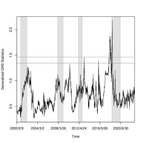
Figure 1: Time-Varying Generalized GRS Statistics

Thus we examine the time instability of the APT in the Japanese stock market using the rolling window method. As mentioned in Section 2, we apply Fama and MacBeth’s (1973) two-step regression with rolling windows to investigate whether the APT is time instable. In the time-varying (rolling window) regression, we set the length of the window width to 500, which is approximately two years. Figure 1 shows the time-varying generalized GRS test statistics for each period.

(Figure 1 around here)

We find that the APT is not valid in the following periods: (1) after April 4, 2013, when the Bank of Japan (BOJ) began quantitative and qualitative monetary easing (QQE), (2) after January 29, 2016, when the BOJ began QQE with a negative interest rate, and (3) after July 31, 2018, when the BOJ allowed the long-term Japanese government bond (JGB) yield to move more volatile. We explore each period on the invalidity of the APT in the following.

First, the most significant cause of the deterioration in the validity of the APT is the BOJ’s decision on July 31, 2018 to allow greater volatility in long-term JGB yields. The unexpected change in the volatility of the long-term JGB yield can significantly affect the price of other financial assets. For instance, Hui et al. (2022) study the bond yield movements under yield curve control. They show that the restoring force in the yield dynamics toward its equilibrium level weakens sharply at the end of September 2018. This result suggests that arbitrage opportunities may arise between financial assets around the periods.

Second, our empirical results show that the introduction of the QQE on April 4, 2013, contributes more to the deterioration of the validity of the APT than the introduction of the QQE with a negative interest rate on January 29, 2016. This result is consistent with Fukuda (2018), who examines the spillover effects of Japan’s negative interest rate policy on Asian stock markets, including the Japanese stock market. He concludes that the impact of QQE with a negative interest rate on the Japanese stock market is limited compared to QQE.

In addition, the time-varying generalized GRS test statistics remain in the range where the null hypothesis is not rejected in other periods. However, we can see that the validity of the APT has been changing relatively because the test statistics also change significantly over time. In particular, there are some periods where the generalized GRS test statistics have high values but cannot reject the null hypothesis in the following periods: (i) the recession period from November 2000 to January 2002, (ii) the period around 2007, when the subprime mortgage problem became apparent, (iii) after October 31, 2014, when the BOJ expanded the QQE, (iv) after December 14, 2016, when the Federal Open Market Committee (FOMC) increased the federal funds rate, and (v) after April 25, 2019, when the BOJ announced the exchange traded funds (ETF) lending facility. Here, we classify these events that affect the behavior of the test statistics into three groups: business cycle, financial crisis, and monetary policy. We can regard these events as exogenous shocks.

In summary, the behavior of the generalized GRS test statistics are not stable over time. It is affected by exogenous shocks such as monetary policy, financial crisis, and the business cycle. In particular, our empirical results show that the monetary policy of manipulating long-term interest rates significantly affects the validity of the APT. Our empirical results are consistent with Inoue and Okimoto (2022a, b). Their studies examine the spillover effects of the Bank of Japan’s and the Federal Reserve’s unconventional monetary policies on domestic and global financial markets in the different sample periods using the smooth-transition global VAR model. They show that the BOJ’s monetary easing increases the Japanese stock price, and the effects on the Japanese stock market are long-lasting regardless of the different sample periods. This implies that the BOJ’s monetary policy changes cause arbitrage opportunities in the Japanese stock market. Moreover, our empirical results are consistent with Noda (2016), who identifies the periods when the Japanese stock market is efficient based on Ito et al.’s (2016; 2022) time-varying autoregressive model. He shows that the efficiency of the Japanese stock market changes in response to the business cycle and exogenous shocks, such as economic crises and wars.

(Figure 2 around here)

Figure 2 shows the time-varying estimates for the risk premiums. We recognize that the behavior of each risk premium is not stable over time and is significantly affected by the business cycle and exogenous shocks such as financial crises, the COVID-19 global pandemic, and the Russian invasion of Ukrainein in 2022. Here, the risk factor whose sign condition is positive (negative) is defined as financial assets complementary (alternative) to stocks. Therefore, our empirical results imply that the relationship between each risk factor and the Japanese sector indices changes over time. The detailed estimation results are summarized below.

First, the time-varying estimates of $\lambda_{MKT}$ is upward (downward) sloping during expansions (recessions). This result is consistent with Bansal et al. (2021), who examine the term structure of expected equity risk premia over time in the U.S., Europe, and Japan. In addition, our empirical results show that the volatilities of $\lambda_{WORLD}$ and $\lambda_{EMERGE}$ increase in response to financial crises. This result is consistent with Choudhry et al. (2007), who examine the changes in the long-run relationships between the stock prices of Far East countries, Japan, and the U.S. around the Asian financial crisis. They suggest that the relationships between the Japanese and other stock markets become closer during financial crises.

Second, we find that the time-varying estimates of $\lambda_{CMD}$ is not statistically significant over the sample periods, but its volatility is significantly affected by exogenous shocks. This result is consistent with Thuraisamy et al. (2013), who investigate the volatility interactions between 14 Asian stock markets, including Japanese stock market, and dominant commodity markets. They show that the shape of volatility dynamics changes during economic crises. Furthermore, Zhang and Hamori (2021) investigate the return and volatility spillover between the COVID-19 pandemic in 2020, the crude oil market, and the stock market. They find that the volatility spillovers between the crude oil and stock markets increase significantly more during the COVID-19 global pandemic than during the global financial crisis. That is why the volatility of $\lambda_{CMD}$ may increase significantly during the COVID-19 global pandemic.

Third, the time-varying estimates of $\lambda_{RP}$ and $\lambda_{UTS}$ are not stable over time, and their behavior is affected by the business cycle. However, there are some differences in the behavior of the estimates in that $\lambda_{RP}$ is more affected by the business cycle than $\lambda_{UTS}$. This result is consistent with Okimoto and Takaoka (2017, 2022), who examine the predictability of the business cycle in Japan using the term structure of credit spreads and the government bond yield spread. Their empirical results show that the term structure of credit spreads is more helpful in predicting the business cycle in Japan than the government bond yield spread.

Fourth, the time-varying estimates of $\lambda_{UYEN}$ is not statistically significant over the sample periods, which is consistent with Hamao (1988), and Tsuji (2007). Moreover, our empirical results reveal that the behavior of $\lambda_{UYEN}$ is significantly affected by changes in monetary policy, and $\lambda_{UYEN}$ converges to zero during the COVID-19 pandemic. This suggests that the UYEN does not contribute to the formation of the risk premium of the Japanese sector indices during the COVID-19 pandemic. Aslam et al. (2020) examine the efficiency of foreign exchange markets during the COVID-19 pandemic. Their empirical results show that the Japanese yen against the U.S. dollar was highly efficient before the COVID-19 pandemic periods, but the efficiency of the exchange rate decreases tremendously during the COVID-19 pandemic. Therefore, the inefficiency of the foreign exchange market may be the reason why the UYEN does not contribute to the appropriate formation of the risk premium in the Japanese sector indices during the COVID-19 pandemic.

Finally, we find that the time-varying estimates of $\lambda_{UI}$ is not statistically significant and stable in many periods. However, the sign condition of $\lambda_{UI}$ becomes negative and the volatility of the estimates increases during the COVID-19 pandemic. We believe that the changes in BOJ’s monetary policy cause the sharp fluctuation of $\lambda_{UI}$. The BOJ enhanced monetary easing on April 27, 2020, in response to the COVID-19 global pandemic. In practice, the BOJ decided to purchase a necessary amount of JGBs, without setting a ceiling, so that the yield on the 10-year JGB would remain around zero percent. This monetary easing, which lasted until March 2023, led to unexpected inflation through a sharp increase in the money supply. As a result, we believe that it had a significant impact on the estimate of $\lambda_{UI}$ and its volatility.

5 Conclusion

This paper is the first study to investigate the time instability of the APT in the Japanese stock market. Previous studies, such as Hamao (1988), Azeez and Yonezawa (2006), and Tsuji (2007), estimate the time-invariant risk premium under the implicit assumption that the market structure is stable over time. Then we employ Fama and MacBeth’s (1973) two-step regression with rolling windows and Kamstra and Shi’s (2023) generalized GRS test to examine the validity of the assumption in the previous studies. In addition, we measure how changes in each risk factor affect the risk premiums in the Japanese stock market based on the above time-varying procedure. Our findings are summarized below.

First, we find that the APT is supported over the entire sample period, but the validity of the APT varies over time in the Japanese stock market. In particular, we find that the effectiveness of the APT is largely affected by the changes in monetary policy, especially the manipulation of long-term interest rates. Moreover, the business cycle and economic crises affect the magnitude of the validity of the APT. Second, we show that the time-varying estimates of the risk premiums for each factor are also unstable over time, and they are affected by the business cycle and economic crises. This implies that the relationship between stock returns and risk factors varies over time. We confirm that each risk factor can be an alternative (complementary) financial asset to stocks, depending on the occasion.

Thus, while previous studies assume that the validity of APT is stable over time, our results suggest that the validity varies over time. We conclude that the implicit assumption of previous studies that the market structure is stable over time is not reasonable.

Table 1: Variable Definitions

Variables	Details	Data Source
Risk Premiums
FAF	TOPIX Fishery, Agriculture & Forestry	Tokyo Stock Exchange
FOD	TOPIX Foods	Tokyo Stock Exchange
MIN	TOPIX Mining	Tokyo Stock Exchange
OIL	TOPIX Oil and Coal Products	Tokyo Stock Exchange
CON	TOPIX Construction	Tokyo Stock Exchange
MET	TOPIX Metal Products	Tokyo Stock Exchange
GLC	TOPIX Glass and Ceramics Products	Tokyo Stock Exchange
TEX	TOPIX Textiles and Apparels	Tokyo Stock Exchange
PUL	TOPIX Pulp and Paper	Tokyo Stock Exchange
CHE	TOPIX Chemicals	Tokyo Stock Exchange
PHA	TOPIX Pharmaceutical	Tokyo Stock Exchange
RUB	TOPIX Rubber Products	Tokyo Stock Exchange
TEQ	TOPIX Transportation Equipment	Tokyo Stock Exchange
IRS	TOPIX Iron and Steel	Tokyo Stock Exchange
NFM	TOPIX Nonferrous Metals	Tokyo Stock Exchange
MAC	TOPIX Machinery	Tokyo Stock Exchange
ELA	TOPIX Electric Appliances	Tokyo Stock Exchange
PRE	TOPIX Precision Instruments	Tokyo Stock Exchange
OTH	TOPIX Other Products	Tokyo Stock Exchange
INF	TOPIX Information & Communication	Tokyo Stock Exchange
SER	TOPIX Services	Tokyo Stock Exchange
ELP	TOPIX Electric Power and Gas	Tokyo Stock Exchange
LTP	TOPIX Land Transportation	Tokyo Stock Exchange
MTP	TOPIX Marine Transportation	Tokyo Stock Exchange
ATP	TOPIX Air Transportation	Tokyo Stock Exchange
WHS	TOPIX Warehousing and Harbor Transportation	Tokyo Stock Exchange
WHO	TOPIX Wholesale Trade	Tokyo Stock Exchange
RET	TOPIX Retail Trade	Tokyo Stock Exchange
BAK	TOPIX Banks	Tokyo Stock Exchange
SEC	TOPIX Securities and Commodities Futures	Tokyo Stock Exchange
INS	TOPIX Insurance	Tokyo Stock Exchange
OFB	TOPIX Other Financing Business	Tokyo Stock Exchange
RES	TOPIX Real Estate	Tokyo Stock Exchange
Risk Factors
MKT	Difference between Returns on TOPIX and Gensaki Rate	Tokyo Stock Exchange and Tanshi Kyokai
WORLD	MSCI World Index (Developed 23 countries)	Morgan Stanley
EMERGE	MSCI Emerging Markets Index (Developing 26 countries)	Morgan Stanley
CMD	Forward Spread between Spot and Three-month S&P GSCI Commodity Index	Standard & Poors
UTS	Yield Spread between 10 year Japanese Government Bonds (JGB) and Gensaki Rate	MOF Japan and Tanshi Kyokai
RP	Credit Spread between S&P 10+years corporate bond and 10 year JGB	Standard & Poors and MOF Japan
UYEN	Forward Premium between the Spot and Three-month Yen/U.S. Dollar Exchange Rates	Bank of Japan and MUFG Bank, Ltd.
UI	Unexpected Inflation Calculated in Accordance with Chen et al. (1986)	Tanshi Kyokai and JP Morgan

• We calculate UTS, RP, UYEN, and UI following Chen et al. (1986).

Table 2: The Estimated and Expected Risk Premiums (Whole Sample)

	Estimated	Expected
$\lambda_{MKT}$	$-0.0007$	$-0.0007$
	[0.0000]
$\lambda_{WORLD}$	$-0.0002$	$-0.0006$
	[0.0011]
$\lambda_{EMERGE}$	0.0009	$-0.0007$
	[0.0005]
$\lambda_{CMD}$	0.0010	$-0.0008$
	[0.0004]
$\lambda_{UTS}$	0.0023	$0.0075$
	[0.0010]
$\lambda_{RP}$	$-0.0026$	$-0.0098$
	[0.0010]
$\lambda_{UYEN}$	$0.0009$	$-0.0008$
	[0.0006]
$\lambda_{UI}$	$-0.0002$	$-0.0008$
	[0.0001]

Notes:

• “Estimated” and “Expected” denote the $\hat{\lambda}_{i}$ and the sample mean ${\mathbb{E}}[\lambda_{i}]$, respectively.

• The robust standard errors for the GLS estimation are shown in brackets.

• R version 4.3.0 was used to compute the estimates and statistics.

Notes:

• The dashed red and blue lines denote the critical value at the 5% and 10% significance levels for the generalized GRS test, respectively.

• The shade areas are recessions as defined by the Cabinet Office Japan “Indexes of Business Conditions.”

• R version 4.3.0 was used to compute the statistics.

Figure 2: Time-Varying Estimates of Risk Premiums

Notes:

• The dashed red lines represent the 95% confidence intervals of the estimates.

• The shade areas are recessions as defined by the Cabinet Office Japan “Indexes of Business Conditions.”

• R version 4.3.0 was used to compute the estimates.

References

- Aslam et al. (2020) Aslam, F., Aziz, S., Nguyen, D. K., Mughal, K. S., and Khan, M. (2020), “On the Efficiency of Foreign Exchange Markets in Times of the COVID-19 Pandemic,” Technological Forecasting & Social Change, 161, 120261.
- Azeez and Yonezawa (2006) Azeez, A. A. and Yonezawa, Y. (2006), “Macroeconomic Factors and the Empirical Content of the Arbitrage Pricing Theory in the Japanese Stock Market,” Japan and the World Economy, 18, 568–591.
- Bansal et al. (2021) Bansal, R., Miller, S., Song, D., and Yaron, A. (2021), “The Term Structure of Equity Risk Premia,” Journal of Financial Economics, 142, 1209–1228.
- Chen et al. (1986) Chen, N., Roll, R., and Ross, S. A. (1986), “Economic Forces and the Stock Market,” Journal of Business, 59, 383–403.
- Choudhry et al. (2007) Choudhry, T., Lu, L., and Peng, K. (2007), “Common Stochastic Trends among Far East stock Prices: Effects of the Asian Financial Crisis,” International Review of Financial Analysis, 16, 242–261.
- Doukas et al. (1999) Doukas, J., Hall, P. H., and Lang, L. H. P. (1999), “The Pricing of Currency Risk in Japan,” Journal of Banking & Finance, 23, 1–20.
- Fama and French (1993) Fama, E. F. and French, K. R. (1993), “Common Risk Factors in the Returns on Stocks and Bonds,” Journal of Financial Economics, 33, 3–56.
- Fama and French (2015) — (2015), “A Five-Factor Asset Pricing Model,” Journal of Financial Economics, 116, 1–22.
- Fama and French (2016) — (2016), “Dissecting Anomalies with a Five-Factor Model,” Review of Financial Studies, 29, 69–103.
- Fama and MacBeth (1973) Fama, E. F. and MacBeth, J. D. (1973), “Risk, Return, and Equilibrium: Empirical Tests,” Journal of Political Economy, 81, 607–636.
- Fukuda (2018) Fukuda, S. (2018), “Impacts of Japan’s Negative Interest Rate Policy on Asian Financial Markets,” Pacific Economic Review, 23, 67–79.
- Gibbons et al. (1989) Gibbons, M. R., Ross, S. A., and Shanken, J. (1989), “A Test of the Efficiency of a Given Portfolio,” Econometrica, 57, 1121–1152.
- Hamao (1988) Hamao, Y. (1988), “An Empirical Examination of the Arbitrage Pricing Theory: Using Japanese Data,” Japan and the World Economy, 1, 45–61.
- Hansen (1982) Hansen, L. P. (1982), “Large Sample Properties of Generalized Method of Moments Estimators,” Econometrica, 50, 1029–1054.
- Hansen et al. (1996) Hansen, L. P., Heaton, J., and Yaron, A. (1996), “Finite-Sample Properties of Some Alternative GMM Estimators,” Journal of Business & Economic Statistics, 14, 262–280.
- Hansen and Jagannathan (1997) Hansen, L. P. and Jagannathan, R. (1997), “Assessing Specification Errors in Stochastic Discount Factor Models,” Journal of Finance, 52, 557–590.
- He and Ng (1998) He, J. and Ng, K. (1998), “The Foreign Exchange Exposure of Japanese Multinational Corporations,” Journal of Finance, 53, 733–753.
- Homma et al. (2005) Homma, T., Tsutsui, Y., and Benzion, U. (2005), “Exchange Rate and Stock Prices in Japan,” Applied Financial Economics, 15, 469–478.
- Hui et al. (2022) Hui, C., Wong, A., and Lo, C. (2022), “A Note on Modelling Yield Curve Control: A Target-Zone Approach,” Finance Research Letters, 49, 103076.
- Inoue and Okimoto (2022a) Inoue, T. and Okimoto, T. (2022a), “How does Unconventional Monetary Policy Affect the Global Financial Markets?” Empirical Economics, 62, 1013–1036.
- Inoue and Okimoto (2022b) — (2022b), “International Spillover Effects of Unconventional Monetary Policies of Major Central Banks,” International Review of Financial Analysis, 79, 101968.
- Ito et al. (2016) Ito, M., Noda, A., and Wada, T. (2016), “The Evolution of Stock Market Efficiency in the US: a Non-Bayesian Time-Varying Model Approach,” Applied Economics, 48, 621–635.
- Ito et al. (2022) — (2022), “An Alternative Estimation Method for Time-Varying Parameter Models,” Econometrics, 10.
- Jagannathan et al. (1998) Jagannathan, R., Kubota, K., and Takehara, H. (1998), “Relationship between LaborâIncome Risk and Average Return: Empirical Evidence from the Japanese Stock Market,” Journal of Business, 71, 319–347.
- Jagannathan and Wang (1996) Jagannathan, R. and Wang, Z. (1996), “The Conditional CAPM and the Cross-Section of Expected Returns,” Journal of Finanace, 51, 3–53.
- Kamstra and Shi (2023) Kamstra, M, J. and Shi, R. (2023), “Testing and Ranking of Asset Pricing Models Using the GRS Statistic,” Available at Social Science Research Network: http://dx.doi.org/10.2139/ssrn.4374415.
- Kaneko and Lee (1995) Kaneko, T. and Lee, B. (1995), “Relative Importance of Economic Factors in the U.S. and Japanese Stock Markets,” Journal of the Japanese and International Economies, 9, 290–307.
- Kim et al. (2011) Kim, J. H., Shamsuddin, A., and Lim, K. P. (2011), “Stock Return Predictability and the Adaptive Markets Hypothesis: Evidence from Century-Long U.S. Data,” Journal of Empirical Finance, 18, 868–879.
- Kubota and Takehara (2018) Kubota, K. and Takehara, H. (2018), “Does the Fama and French Five-Factor Model Work Well in Japan?” International Review of Finance, 18, 137–146.
- Lintner (1965) Lintner, J. (1965), “The Valuation of Risk Assets and the Selection of Risky Investments in Stock Portfolios and Capital Budgets,” Review of Economics and Statistics, 47, 13–37.
- Merton (1973) Merton, R. C. (1973), “An Intertemporal Capital Asset Pricing Model,” Econometrica, 41, 867–887.
- Noda (2016) Noda, A. (2016), “A Test of the Adaptive Market Hypothesis using a Time-Varying AR Model in Japan,” Finance Research Letters, 17, 66–71.
- Okimoto and Takaoka (2017) Okimoto, T. and Takaoka, S. (2017), “The Term Structure of Credit Spreads and Business Cycle in Japan,” Journal of the Japanese and International Economies, 45, 27–36.
- Okimoto and Takaoka (2022) — (2022), “The Credit Spread Curve Distribution and Economic Fluctuations in Japan,” Journal of International Money and Finance, 122, 102582.
- Ren and Shimotsu (2009) Ren, Y. and Shimotsu, K. (2009), “Improvement in Finite Sample Properties of the HansenâJagannathan Distance Test,” Journal of Empirical Finance, 16, 483–506.
- Roll (1977) Roll, R. (1977), “A Critique of the Asset Pricing Theory’s Tests Part I: On Past and Potential Testability of the Theory,” Journal of Financial Economics, 4, 129–176.
- Ross (1976) Ross, S. A. (1976), “The Arbitrage Theory of Capital Asset Pricing,” Journal of Economic Theory, 13, 341–360.
- Sargan and Bhargava (1983) Sargan, J. D. and Bhargava, A. (1983), “Maximum Likelihood Estimation of Regression Models with First Order Moving Average Errors when the Root Lies on the Unit Circle,” Econometrica, 51, 799–820.
- Schwarz (1978) Schwarz, G. (1978), “Estimating the Dimension of a Model,” Annals of Statistics, 6, 461–464.
- Shanken (1992) Shanken, J. (1992), “On the Estimation of Beta-Pricing Models,” Review of Financial Studies, 5, 1–33.
- Sharpe (1964) Sharpe, W. F. (1964), “Capital Asset Prices: A Theory of Market Equilibrium under Conditions of Risk,” Journal of Finance, 19, 425–442.
- Silvennoinen and Thorp (2013) Silvennoinen, A. and Thorp, S. (2013), “Financialization, Crisis and Commodity Correlation Dynamics,” Journal of International Financial Markets, Institutions & Money, 24, 42–65.
- Thorbecke (2020) Thorbecke, W. (2020), “How the Coronavirus Crisis Affected Japanese Industries: Evidence from the Stock Market,” RIETI Discussion Paper Series 20-E-061.
- Thuraisamy et al. (2013) Thuraisamy, K. S., Sharma, S. S., and Ahmed, H. J. A. (2013), “The Relationship between Asian Equity and Commodity Futures Markets,” Journal of Asian Economics, 28, 67–75.
- Tsuji (2007) Tsuji, C. (2007), “What Macro-Innovation Risks Really Are Priced in Japan ?” Applied Financial Economics, 17, 1085–1099.
- Zhang and Hamori (2021) Zhang, W. and Hamori, S. (2021), “Crude Oil Market and Stock Markets during the COVID-19 Pandemic: Evidence from the US, Japan, and Germany,” International Review of Financial Analysis, 74, 101702.