Competition between lanes and transient jammed clusters in driven binary mixtures

Abstract

We consider mixtures of oppositely driven particles, showing that their non-equilibrium steady states form lanes parallel to the drive, which coexist with transient jammed clusters where particles are temporarily immobilised. We analyse the interplay between these two types of non-equilibrium pattern formation, including their implications for macroscopic demixing perpendicular to the drive. Finite-size scaling analysis indicates that there is no critical driving force associated with demixing, which appears as a crossover in finite systems. We attribute this effect to the disruption of long-ranged order by the transient jammed clusters.

Non-equilibrium systems can form complex patterns in their steady states, including flocking of birds [1, 2, 3], active nematics [4, 5], and motility-induced phase separation [6, 7, 8]. These patterns are sustained by the continuous injection of energy into the system, which is then dissipated as heat. In some systems, the formation and evolution of large coherent structures can be captured by deterministic equations [9, 10, 11], while others support chaotic fluctuating patterns that necessitate a stochastic description, using methods of non-equilibrium statistical physics. Such systems are challenging for state-of-the-art theories: How should emergent patterns be measured and classified? Can one identify distinct dynamical phases, by analogy with equilibrium systems? Can the patterns be shaped and controlled by external perturbations?

A common example of a fluctuating pattern is the emergence of lanes, when two species of particles are driven in opposite directions: particles which are driven in the same direction tend to follow each other. In physics, this occurs for colloidal systems in electric fields [12, 13, 14], and in plasmas [15, 16, 17, 18], and ionic liquids [19]. Similar structures are also familiar from pedestrian flow [20, 21, 22, 23, 24], and ant foragers [25]. Oscillatory electric fields can also induce other patterns in colloidal systems [26, 27, 28]. For colloidal systems with moderate driving fields, the resulting lanes fluctuate stochastically in time: they may extend over large length scales parallel to the field, while their widths are only a few particle diameters.

Laning behaviour can be captured by simulation models where particles interact by repulsive short-ranged potentials and move by Brownian dynamics. These simplified models neglect experimental aspects such as hydrodynamic interactions and electrostatics, but they capture the main features of the experiments, indicating that laning is a robust collective phenomenon, amenable to the methods of statistical physics.

A generic mechanism for laning is enhanced lateral diffusion (ELD) [29, 30, 31, 32, 33, 34, 35]: collisions between oppositely driven particles promote rapid diffusive motion perpendicular to the field. This favours accumulation in lanes, where such collisions are avoided. Previous work has characterised some of the length scales that develop in these non-equilibrium steady states, but open questions remain about the existence (and nature) of long-ranged order, and the possible de-mixing of the system into domains, perpendicular to the drive [36, 37, 32, 38, 35].

In this work, we present computer simulations of a model system that exhibits laning. Details are given below, but we outline the main phenomenology in Fig. 1. Red and blue particles are driven in opposite directions: the driving strength is characterised by the Peclet number (Pe). Increasing Pe from zero, one observes increasingly inhomogeneous steady states (labelled II-IV), which may be contrasted with the homogeneous equilibrium mixture at $\mathrm{Pe}=0$ (state I).

We present three main results: (i) The fully demixed state IV occurs in finite systems but sufficiently large systems are always mixed: there is no long-ranged order perpendicular to the drive. (ii) The large density fluctuations in states II,III can be characterised as transient jammed clusters (TJCs), which tend to disrupt the lanes. (iii) The disruptive effect of TJCs is responsible for the instability of the demixed state. Result (i) extends previous work [36], which drew a similar conclusion about long-ranged order parallel to the drive; the conclusion that sufficiently large systems are always mixed is greatly extended here by the identification of TJCs as the mechanism by which the order is disrupted. Based on these results, we interpret the full phenomenology of colloidal laning as a combination of ELD and transient clustering: the former favours lane formation and long-ranged correlation, while the latter disrupts it. Similar competing effects may also be relevant in other non-equilibrium steady states [39, 40, 41, 42].

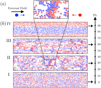
Figure 1: (a) Example of a transient jammed cluster. (b) Steady state configurations of a system with $L_{\parallel}=150d_{0}$, varying $\mathrm{Pe}$, as shown.

Model – We consider a binary mixture of $N$ colloidal particles, with $N/2$ in each species, occupying a two dimensional box of size $L_{\parallel}\times L_{\perp}$, with periodic boundary conditions. The two species have equal and opposite charges: particle $i$ has charge $\sigma_{i}=\pm 1$. Particles are driven by a constant external field $E$ along the $x$-axis and interact with each other via WCA potentials [43], $V(r)=4\epsilon[(d_{0}/r)^{12}-(d_{0}/r)^{6}+(1/4)]\Theta(2^{1/6}d_{0}-r)$, where $d_{0}$ is the diameter, $\epsilon$ is the repulsion strength, and $\Theta$ is the Heaviside function. The position $\bm{r}_{i}=(x_{i},y_{i})$ of particle $i$ follows Langevin dynamics:

$$m\ddot{\bm{r}}_{i}=-\gamma\dot{\bm{r}}_{i}-\nabla_{i}U+\sigma_{i}E\bm{\hat{x}}+\sqrt{2\gamma k_{B}T}\,\bm{\eta}_{i},$$ (1)

where $\gamma$ is a friction constant, $T$ is the temperature of the heat bath, $k_{B}$ is Boltzmann’s constant, $U$ is the interaction energy, and $\bm{\eta}_{i}$ is a Gaussian white noise with mean zero and $\langle{\eta}_{i,\alpha}(t){\eta}_{j,\beta}(t^{\prime})\rangle=\delta_{ij}\delta_{\alpha\beta}\delta(t-t^{\prime})$, where $\alpha,\beta$ indicate Cartesian components. An important time scale for diffusive particle motion is the Brownian time $\tau_{\rm B}=d_{0}^{2}\gamma/(k_{B}T)$.

We non-dimensionalise the system using base units $d_{0},m,\epsilon$ (see Appendix). The remaining dimensionless parameters are the Peclet number $\text{Pe}=Ed_{0}/(k_{B}T)$, the area fraction $\phi=N\pi d_{0}^{2}/(4L_{\parallel}L_{\perp})$, the reduced friction $\tilde{\gamma}=\gamma d_{0}/\sqrt{m\epsilon}$, the reduced temperature $\tilde{T}=k_{\rm B}T/\epsilon$ and the aspect ratio of the simulation box $S=L_{\parallel}/L_{\perp}$. We take $\tilde{\gamma}=1000$ to mimic a high-friction colloidal environment, and $\tilde{\epsilon}=1$ (results depend weakly on this parameter). We vary Pe between 0 and $100$; since particles explore space much more quickly in the $x$-direction, we take $S=5$, except where explicitly stated otherwise. We take $\phi=0.35$ which is representative of the laning regime. The simulations are performed using LAMMPS [44], see Appendix for details.

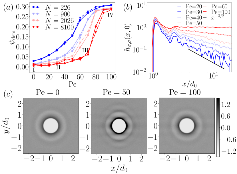
Figure 2: (a) $\psi_{\rm dem}$ against Pe at different system sizes. Dotted and solid lines are obtained from disordered and demixed initial conditions, respectively. (b) $h_{\sigma,\sigma}(\bm{r})$ plotted along the $x$-direction. The solid line indicates $h_{\sigma,\sigma}(x,0)\sim x^{-3/2}$. (c) Dependence of $h_{\rho,\rho}(\bm{r})$ on $\bm{r}=(x,y)$. In (b,c), $L_{\parallel}=150d_{0}$.

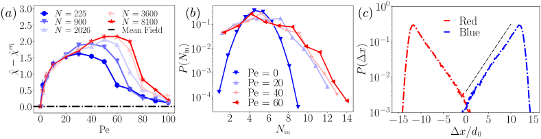
Figure 3: (a) $\tilde{\chi}-\tilde{\chi}^{\text{eq}}$ against Pe, for different system sizes, with cut-off radius $R=5d_{0}$. The mean-field theory predicts that this quantity vanishes for $R\to\infty$. (b) Probability distribution for the number of particles in a circular probe region of radius $r_{0}=1.75d_{0}$ at different Pe. (c) Probability distribution of $\Delta x(\tau)$ for $\tau=0.25\tau_{B}$, at $\text{Pe}=50$. The dashed line indicates $P(\Delta x)\propto e^{-(\Delta x_{\text{free}}-\Delta x)/\ell}$. For (b,c), $L_{\parallel}=300d_{0}$.

We analysed the non-equilibrium steady state of this model for a range of Pe, as shown in Fig. 1(b). We verified that all systems have converged to their steady states by starting independent simulations from both homogeneous and fully de-mixed initial conditions, which lead to the same results. This requires long simulations, up to $4000\tau_{B}$.

Demixing as a smooth crossover – To characterise the fully demixed state, we evaluate the Fourier transform of the charge density at $\bm{k}^{*}=(0,2\pi/L_{\perp})$ [45, 46, 35]:

$$\psi_{\rm dem}=\langle|\Psi({\bm{k}}^{*})|\rangle=\Big{\langle}\Big{|}\frac{1}{L_{\perp}L_{\parallel}}\sum_{i=1}^{N}\sigma_{i}e^{-i\bm{k}^{*}\cdot\bm{r}_{i}}\Big{|}\Big{\rangle},$$ (2)

Here and throughout, angle brackets indicate averages in the steady state of the dynamics.

We use $\psi_{\rm dem}$ as an order parameter for demixing, in a finite-size scaling analysis. This is performed by increasing $N,L_{\parallel},L_{\perp}$, at fixed $\mathrm{Pe},\phi$, and aspect ratio $S$. A demixing phase transition would manifest as a critical Peclet number $\mathrm{Pe}^{*}$: For $\mathrm{Pe}<\mathrm{Pe}^{*}$ the state would be homogeneous and $\Psi({\bm{k}}^{*})$ would be small in modulus (of order $N^{-1/2}$ as $N\to\infty$). For $\mathrm{Pe}>\mathrm{Pe}^{*}$ the state would be demixed: the complex number $\Psi({\bm{k}}^{*})$ has a modulus of order $1$ as $N\to\infty$; its phase is random and indicates the relative positions of the two domains. Hence, demixing involves spontaneous symmetry breaking, via the phase of $\Psi$.

The finite-size scaling results in Fig. 2(a) are not consistent with any such transition. For each system size, there is a crossover from homogeneous to de-mixed states on increasing $\mathrm{Pe}$. However, increasing $N$ shows that ever larger values of $\mathrm{Pe}$ are required to see demixing: there is no sharp threshold $\mathrm{Pe}^{*}$ at which long-ranged order appears. Fig. 2(a) shows that these results are independent of whether the system is initialised in a homogeneous (mixed) or fully demixed state.

Fig. 2(a) suggests a correlation length that grows with $\mathrm{Pe}$ but never diverges: demixing occurs in finite systems when this correlation length reaches $L_{\perp}$. A similar scenario was proposed in [36] by analyzing correlations parallel to the drive. Here we consider correlations in the perpendicular direction, focussing on the system-spanning domains that appear in state IV, and using the order parameter $\psi_{\rm dem}$. Compared with equilibrium phase separation, this result – of demixing in large finite systems without any phase transition – is an unusual feature of these non-equilibrium steady states.

Spatial correlations – States II and III of Fig. 1 exhibit laning, but the particle density also develops inhomogeneities, where right- and left-moving particles tend to block each other. To investigate these correlations in real space, define density-density and charge-charge correlation functions:

$$h_{\rho,\rho}(\bm{r}) =\langle\rho(\bm{{r}})\rho(\bm{{0}})\rangle/\overline{\rho}^{2}-1$$ (3)

$$h_{\sigma,\sigma}(\bm{{r}}) =\langle\sigma(\bm{{r}})\sigma(\bm{{0}})\rangle/\overline{\rho}^{2}$$

where $\rho(\bm{r})=\sum_{i=1}^{N}\delta(\bm{r}_{i}-\bm{r})$ is the empirical particle density, $\sigma(\bm{r})=\sum_{i=1}^{N}\sigma_{i}\delta(\bm{r}_{i}-\bm{r})$ is the charge density, and $\bar{\rho}=N/(L_{\parallel}L_{\perp})$ is the mean density.

The behaviour of these correlation functions on hydrodynamic length scales has been analysed [47, 48, 38, 49] within a mean-field approximation. This approximation is accurate when density fluctuations are not too large, for example at high density with weakly interacting particles [48]. For the system considered here, the particles have strongly repulsive cores and Fig. 1 shows that density fluctuations are large. Hence mean-field theory is not expected to be quantitative: it does not predict the demixing effect seen in state IV. Still, the universal hydrodynamic correlations of [48] should emerge on large scales, within homogeneous states. Fig. 2(b) shows the charge autocorrelation function measured parallel to the drive. For $\mathrm{Pe}=20$, this decays as $|x|^{-3/2}$, consistent with [48]. For larger Pe, the correlations grow smoothly with Pe, as the lanes become more pronounced.

Transient jammed clusters (TJCs) – States II,III in Fig. 1 show strikingly large density fluctuations. Closer inspection reveals transient clusters that contain groups of particles with opposite charge, which block each others’ motion, leading to a transient jamming phenomenon. We now quantify these TJCs and discuss their consequences.

Fig. 2(c) shows density correlations for $\mathrm{Pe}=(0,50,100)$, corresponding to states I,III,IV in Fig. 1(b). For $\mathrm{Pe}=0$ the correlations are isotropic and short-ranged, as expected for an equilibrium fluid. For $\mathrm{Pe}=50$, the correlations are stronger (as indicated by the darker shading) and they are also longer ranged – this is a signature of the TJCs. For $\mathrm{Pe}=100$ the correlations resemble those for $\mathrm{Pe}=0$. This re-entrant behaviour occurs because the demixed domains are similar to equilibrium systems that are being advected at a constant velocity.

To further quantify the TJCs, we integrate the correlation function over space. This result is analogous to the compressibility of an equilibrium system [50], which characterises the size of the density fluctuations:

$$\tilde{\chi}=1+\overline{\rho}\int_{|\bm{r}|<R}h_{\rho,\rho}(\bm{r})d\bm{r}\;.$$ (4)

The large-distance cutoff $R$ reduces statistical uncertainty, results depend weakly on $R$ (see Appendix).

Fig. 3(a) shows $\tilde{\chi}$, measured relative to its equilibrium value. It grows rapidly as Pe increases from zero, indicating the formation of TJCs. There is a plateau at intermediate Pe, showing that these clusters persist across broad range of Pe. Finally, $\tilde{\chi}$ decreases again at large Pe: this is due to demixing, consistent with the re-entrance in Fig. 2(c). The mean-field theory of [48] does not capture these TJCs, because of its assumption of small density fluctuations. For example, the correlations predicted by that theory lead to $\tilde{\chi}\to 0$ as $R\to\infty$, which is not consistent with the data, see Appendix.

As an alternative characterisation of TJCs, Fig. 3(b) shows the probability distribution of the number of particles $N_{\rm in}$ in a spherical probe region [51, 41, 52]. The variance of this distribution increases dramatically with $\mathrm{Pe}$, with tails at large $N_{\rm in}$ reflecting the existence of TJCs. These clusters also have a dynamical signature: Fig. 3(c) shows the distribution of particle displacements parallel to the driving field, for the two species. The distributions are skewed, with significant weight near zero displacement: these are particles which are remain almost stationary in TJCs. Fitting the tail as an exponential with correlation length $\ell$, we estimate a typical time for which particles are immobilised as $\tau_{\rm TJC}=\ell\tau_{\rm B}/(d_{0}{\rm Pe})\approx 0.1\tau_{\rm B}$ (see Appendix): for comparison, the time for a particle to move its diameter within a lane is approximately $\tau_{\rm B}/\mathrm{Pe}\approx 0.02\tau_{\rm B}$, so the slowing-down effect is significant. Similar slowing down has been observed in $3d$ [53, 54, 55].

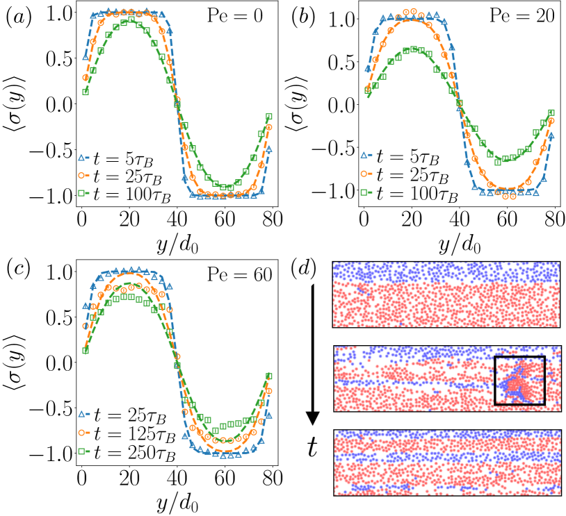
Figure 4: (a,b,c) Time evolution of the charge density profile, starting from a demixed state, for $L_{\parallel}=100d_{0}$ and $S=1.25$. (d) Time series, highlighting a TJC that nucleates new lanes. We show a subsystem from large simulation with $L_{\parallel}=300d_{0}$ and ${\rm Pe}=80$.

Role of TJCs in mixing – Fig. 2 indicates that these driven systems are always mixed in the limit of large systems; we have also shown that the mixed state supports large TJCs. We now establish a connection between these two results, analysing the mechanism by which de-mixed states become unstable at large $\mathrm{Pe}$.

To achieve this, we initialise systems in demixed states, for parameters such that the steady state is mixed. To collect good statistics while maintaining $L_{\perp}$ large enough for the following analysis, we reduce the aspect ratio to $S=1.25$. Fig. 4 shows composition profiles perpendicular to the drive, for various Pe. In the absence of driving ($\mathrm{Pe}=0$), mixing happens by diffusion. To illustrate this, we fit the results to the (analytical) solution of the diffusion equation $\partial_{t}\langle\sigma\rangle=D_{y}\partial_{y}^{2}\langle\sigma\rangle$, using $D_{y}$ as a single fitting parameter (see Appendix). The fit is excellent. For $\mathrm{Pe}=20$, the system still mixes readily: In this case, the diffusion equation still fits the data adequately but the value of $D_{y}$ is larger, reflecting the enhanced lateral diffusion [32, 35].

However, for $\mathrm{Pe}=60$, the lifetime of the demixed state is longer: the interface between the two domains is stable on short time scales, because collisions between oppositely charged particles tend to deflect them back into their own domains. On longer time scales, mixing does still occur, but the mechanism is not diffusive: this is signalled by systematic deviations from the diffusive theory in Fig. 4(c). In particular, the composition inside the demixed domains relaxes more quickly than diffusive mixing would predict, indicating that a collective mechanism is disrupting the domains.

The mechanism for mixing at high $\mathrm{Pe}$ is illustrated in Fig. 4(d): collisions near the interface occasionally form TJCs which disrupt the flow. This leads to nucleation of two new lanes. Continuing the process, further TJCs will form, generating more lanes, eventually mixing the system. This unusual mechanism further emphasizes the rich phenomenology of these non-equilibrium systems.

One way to understand the absence of demixed states in large systems is that increasing $L_{\parallel}$ provides more locations where TJCs can form, initiating the instability. This mechanism is intrinsic to the interface between the oppositely-moving domains: for example increasing $L_{\perp}$ (at fixed $L_{\parallel}$) does not change the local behaviour near the interface (see Appendix). In other words, the absence of de-mixed states for large $L_{\parallel}$ depends weakly on the aspect ratio of the system, since any interface between counterpropagating domains is prone to fragmentation via TJCs. Interfaces between oppositely-driven domains have been recently studied in [56, 57], and nucleation of lanes is also reminiscent of other complex flow phenomena [58].

Interestingly, if the system is small enough that the steady state is fully demixed, the mechanism of Fig. 4(d) can also operate in reverse: four lanes can merge into two, because of a TJC that forms at the interface (see Appendix). However, for large systems, it is the mixing (lane creation) events that predominate.

Outlook – Lane formation for oppositely driven particles relies on enhanced lateral diffusion, which tends to cause demixing, perpendicular to the drive. We showed that this demixing is not a sharp phase transition – sufficiently large systems always remain mixed. They also support large density fluctuations in the form of TJCs, which exist over a wide range of Pe, and play an important role in stabilising the homogeneous (mixed) states, by destabilising interfaces between domains with oppositely driven particles. In this sense, the complex patterns shown in Fig. 1 reflect a competition between ordering by enhanced lateral diffusion and mixing via TJCs. We look forward to future work on such patterns – for example, the possibility of system-spanning TJCs may be relevant for dynamical arrest in small systems [59], and similar phenomena may also be relevant for systems where particles are driven by self-propulsive forces or shear flow, instead of external fields [60, 39, 61, 41, 62, 40, 42]. At higher densities, we also anticipate an interesting interplay between TJCs and crowding (or glassy) behaviour [63, 64].

 

Appendix A APPENDIX

Appendix B 1. Model and simulation details

– Non-dimensionalisation of Langevin Equation

We non-dimensionalise the Langevin equation (1) using base units $d_{0},m,\epsilon$. The natural unit of time is $t_{0}=d_{0}\sqrt{m/\epsilon}$. Then we define reduced quantities which are: the particle position $\tilde{\bm{r}}_{i}=\bm{r}_{i}/d_{0}$, the Peclet number $\text{Pe}=Ed_{0}/(k_{\rm B}T)$, the volume fraction $\phi=N\pi d_{0}^{2}/(4L_{\parallel}L_{\perp})$, the reduced time $\tilde{t}=t/t_{0}$, the reduced electric field $\tilde{E}=Ed_{0}/\epsilon$, the reduced interaction energy $\tilde{U}=U/\epsilon$, the reduced friction constant $\tilde{\gamma}=\gamma t_{0}/m$, the reduced temperature $\tilde{T}=k_{\rm B}T/\epsilon$, and the aspect ratio of the simulation box $S=L_{\parallel}/L_{\perp}$. Recall that the Brownian time is $\tau_{\rm B}=d_{0}^{2}\gamma/(k_{B}T)=t_{0}\tilde{\gamma}/\tilde{T}$: this evaluates to $10^{3}t_{0}$ for the parameters used in this work.

The non-dimensionalised Langevin equation is then

$$\frac{d^{2}}{d\tilde{t}^{2}}\tilde{\bm{r}}_{i}=-\tilde{\gamma}\frac{d}{d\tilde{t}}\tilde{\bm{r}}_{i}-\tilde{\nabla}_{i}\tilde{U}+\sigma_{i}\tilde{E}\hat{\bm{x}}+\sqrt{2\tilde{\gamma}\tilde{T}}\,\tilde{\bm{\eta}}_{i}(\tilde{t}),$$ (5)

where $\tilde{\bm{\eta}_{i}}$ is non-dimensionalised Gaussian white noise with mean zero and $\langle\tilde{{\eta}}_{i,\alpha}(\tilde{t})\tilde{{\eta}}_{j,\beta}(\tilde{t}^{\prime})\rangle=\delta_{ij}\delta_{\alpha\beta}\delta(\tilde{t}-\tilde{t}^{\prime})$.

– Simulation Details

Simulations are performed in LAMMPS [44] with time step $\delta t=5\times 10^{-4}t_{0}$. For initialisation, we either use disordered or demixed initial conditions. For the disordered case, we initialise $N/2$ red and $N/2$ blue particles with random positions and simulate the equilibrium system ($E=0$) for $10^{2}\tau_{B}$, after which the field $E$ is introduced. For the demixed case, we initialise $N$ particles of a single type with random positions and simulate the equilibrium system for $10^{2}\tau_{B}$. Then we assign types to particles according to their $y$-coordinates: for $y_{i}\in[0,L_{\perp}/2]$ we take $\sigma_{i}=-1$ and for $y_{i}\in[L_{\perp}/2,L_{\perp}]$ we take $\sigma_{i}=1$. Then we turn on the field $E$. As discussed in the main text, the steady state of the system is independent of whether disordered or demixed initialisation is used, and all measurements are taken in steady state.

For Fig. 1, Fig. 2, and Fig. 3, the steady state measurements are performed after simulation for at least $10^{3}\tau_{B}$, so that the system has relaxed to its steady state. We confirm the steady state behavior by comparing the simulations performed with both disordered and demixed initial conditions. When the system phase separate, the coarsening process is extremely slow as the interfaces are smooth and stable. When $\text{Pe}>90$, it takes approximately $4\times 10^{3}\tau_{B}$ for system to reach complete phase separation, and results are collected after this time.

For Fig. 3(c), the longitudinal displacement of particle $i$ in time $\tau$ is measured as

$$\Delta x_{i}(\tau)=x_{i}(t_{0}+\tau)-x_{i}(t_{0}),$$ (6)

where $t_{0}$ is an arbitrary initial time.

Appendix C 2. Generalised compressibility $\tilde{\chi}$

– Dependence on cutoff $R$

In the main text, we defined $\tilde{\chi}$ in terms of the density fluctuations of the system. In equilibrium systems, this $\tilde{\chi}$ is related to the compressibility (defined in terms of dependence of the volume on the applied pressure). In these non-equilibrium systems there is no relation between $\tilde{\chi}$ and responses to applied pressure, so we refer to it as a generalised compressibility.

To parameterise the cutoff in Eq. 4, we non-dimensionalise as $\tilde{R}=R/d_{0}$. For the main text, we take $\tilde{R}=5$ to reduce numerical uncertainties. In Fig. 5, we show that the behavior of $\tilde{\chi}$ depends weakly on this cutoff. There is a small increase on increasing $\tilde{R}$, from the tails of $h_{\rho,\rho}$ but the robust qualitative feature is that $\tilde{\chi}$ increases strongly with $\rm Pe$, saturates at a plateau, and then decreases.

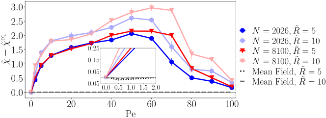
Figure 5: Generalised compressibility $\tilde{\chi}-\tilde{\chi}^{\text{eq}}$ against Pe at $L_{\parallel}=150d_{0}$, $L_{\parallel}=300d_{0}$ with $\tilde{R}=5,10$. The mean-field curves are shown with $\tilde{v}_{0}=1$, see the text for a discussion.

– Mean-field analysis

We describe here the mean-field prediction for density-density correlations, see also Fig. 3(a) of the main text. From [48] one obtains the hydrodynamic (or singular) part of the density-density correlation function which we denote as $h^{s}_{\rho,\rho}(x,y)$. This hydrodynamic correlation is valid on large length scales but it misses effects of particle packing, for example one has $h^{s}=0$ for the equilibrium case $\mathrm{Pe}=0$ (although of course $h\neq 0$ in this case). Hence we subtract the equilibrium part of $\tilde{\chi}$ when comparing the numerical results with the theory.

The singular part of the correlation function in two spatial dimensions can be obtained from [48] as

$$h^{s}_{\rho,\rho}(x,y)=\mathrm{Pe}^{1/2}\frac{H_{\rho,\rho}}{|x|^{3/2}}\left(\frac{\text{Pe}\,y^{2}}{{\cal D}|x|}-1\right)\exp\left(-\frac{\mathrm{Pe}\,y^{2}}{{2\cal D}|x|}\right),$$ (7)

where $H_{\rho,\rho}$ and ${\cal D}$ are constants that are fully determined by a single parameter of the model, which is the Fourier transform of the interaction potential evaluated at wavevector $k=0$. This parameter is denoted $\tilde{v}_{0}$. We always have ${\cal D}>0$; for $\tilde{v}_{0}\lesssim 1.3$ then $H_{\rho,\rho}>0$ while for larger $\tilde{v}_{0}$ we have $H_{\rho,\rho}<0$.

We integrate the singular part of the density correlation function to get the singular part of the generalised compressibility, $\tilde{\chi}^{s}_{\text{mean-field}}=\overline{\rho}\int_{|{\bm{r}}|<R}h^{s}_{\rho,\rho}({\bm{r}})d{\bm{r}}$. We obtain

$$\tilde{\chi}^{s}_{\text{mean-field}}=\overline{\rho}H_{\rho,\rho}\text{Pe}^{1/2}\int^{R}_{0}\int^{\sqrt{R^{2}-x^{2}}}_{0}\frac{1}{x^{3/2}}\left(\frac{\text{Pe}\,y^{2}}{2{\cal D}x}-1\right)\exp\left({-\frac{\text{Pe}\,y^{2}}{2{\cal D}x}}\right)dydx\;.$$ (8)

Integrate $y$ by parts, and make change of variable $u=x/R$ to simply the integral:

$$\tilde{\chi}^{s}_{\text{mean-field}} =-\overline{\rho}H_{\rho,\rho}\sqrt{\text{Pe}/R}\int^{1}_{0}\frac{\sqrt{1-u^{2}}}{u^{3/2}}\exp\left[{\frac{\text{Pe}\,R}{2{\cal D}}\left(u-\frac{1}{u}\right)}\right]du$$ (9)

This final integral is easily computed numerically. Moreover, the argument of the exponential is always negative so one sees that $\tilde{\chi}^{s}_{\text{mean-field}}\to 0$ as the cutoff $R\to\infty$. Fig. 5 shows the $R$-dependence of results from simulation, showing that $\tilde{\chi}$ increases weakly with $R$, contrary to this prediction. (Agreement is not expected here, because the mean-field theory does not capture large density fluctuations such as TJCs.)

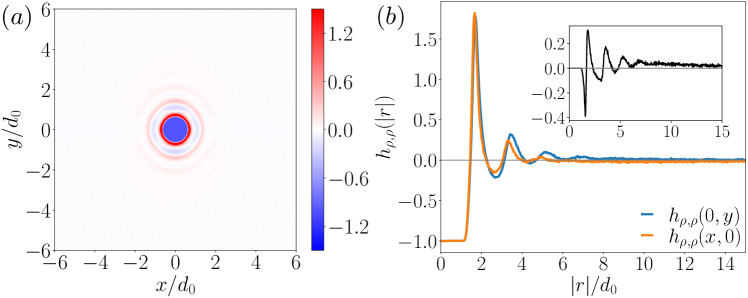
Figure 6: (a) Dependence of $h_{\rho,\rho}(\bm{r})$ on $\bm{r}=(x,y)$. (b) The density-density correlation function $h_{\rho,\rho}(0,y)$ and $h_{\rho,\rho}(x,0)$. The inset is the difference $h_{\rho,\rho}(0,y)-h_{\rho,\rho}(x,0)$. The sign of $h_{\rho,\rho}(0,y)-h_{\rho,\rho}(x,0)$ suggests $H_{\rho,\rho}>0$ in the mean-field theory. For both (a,b), $L_{\parallel}=150d_{0}$ and $\rm Pe=20$.

For a more detailed analysis, Fig. 6 shows the behaviour of $h_{\rho,\rho}$ for ${\rm Pe}=20$. In particular, we show the behaviour along the axes $\bm{r}=(x,0)$ and $\bm{r}=(0,y)$. For the latter case, Eq. 7 predicts that the hydrodynamic part of the correlation is exponentially small but the numerical results show a small but positive contribution that decays slowly at large scales. (We attribute this to TJCs that are extended along the $y$-direction, which are not accounted for by mean-field theory.) Since $h_{\rho,\rho}(x,0)<0$ at large distances while $h_{\rho,\rho}(0,y)>0$, the best chance for agreement with (7) is to take $H_{\rho,\rho}>0$, indicating $\tilde{v}_{0}<1.3$. The mean-field results are obtained with $\tilde{v}_{0}=1$, however, this leads to $\tilde{\chi}^{s}_{\text{mean-field}}<0$, see Fig. 5 (recall also that this $\tilde{\chi}^{s}_{\text{mean-field}}\to 0$ for large $R$).

Appendix D 3. Residence Time for Particles in TJCs

As described in the main text, the characteristic trapping time of particles in TJCs can be estimated from the distribution of longitudinal displacement in Fig. 3(c), using the following simple model. The measurement window for the displacement is $\tau$ and we consider the species with positive charge, so a free particle (outside of the TJC) travels an average distance approximately $\Delta x_{\text{free}}=\tau E/\gamma$ within this time. (The average velocity of a free particle is $v_{\text{free}}=E/\gamma$.)

From Fig. 3(c), the distribution of displacements $P(\Delta x)$ has an exponential tail for small $\Delta x$, we write

$$P(\Delta x)\approx Ae^{-(\Delta x_{\text{free}}-\Delta x)/\ell}$$ (10)

where $A$ is a constant and $\ell$ is a characteristic length scale, which is an estimate of the length by which a typical particle in a TJC is “held back” by its temporary immobilisation. (The value of $A$ presumably depends on how many particles participate in TJCs.) As a simple method to obtain a characteristic trapping time we divide $\ell$ by the characteristic velocity to obtain $\tau_{\rm TJC}=\ell/v_{\text{free}}$.

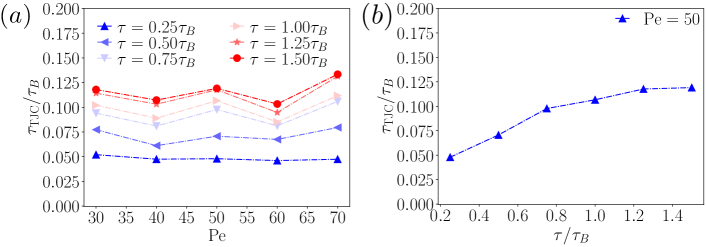
Figure 7: (a) The characteristic trap time $\tau_{\rm TJC}$ in units of $\tau_{B}$ at different $\rm Pe$ number when TJCs are present with $L_{\parallel}=300d_{0}$. (b) The characteristic trapping time $\tau_{\rm TJC}$ against measurement window $\tau$. The characteristic trap time $\tau_{\rm TJC}$ converges with sufficiently large measurement window $\tau$.

To better interpret this time scale, suppose that particles in TJCs stay there for an exponentially distributed time $t_{\rm TJC}$ with mean $\tau_{\rm TJC}$, during which time they do not move at all parallel to the field. Their resulting displacement is then $\Delta x_{\rm free}-v_{\text{free}}t_{\rm TJC}$. Assuming also that $P(t_{\rm TJC})\propto{\rm e}^{-t_{\rm TJC}/\tau_{\rm TJC}}$, the tail of the displacement distribution is readily seen to be (10) with $\ell=\tau_{\rm TJC}v_{\text{free}}=\tau_{\rm TJC}d_{0}{\rm Pe}/\tau_{\rm B}$.

However, this simple analysis neglects effects of the measurement time window $\tau$. In particular, the distribution of $\Delta x$ is not sensitive to trapping times longer than $\tau$. As a result, the above argument tends to underestimate the trapping time. Fig. 7(a) shows the resulting $\tau_{\rm TJC}$ in the regime $\rm Pe\in[30,70]$. These results indicate that large measurement times $\tau$ can be used to obtain robust estimates for the trapping time. Specifically, taking $\text{Pe}=50$ and $\tau=\tau_{B}$, we obtained $\ell=5.4d_{0}$ from the exponential fit and therefore have $\tau_{\rm TJC}=0.11\tau_{B}$. While this is smaller than the Brownian time, it is significantly larger than the the time for a particle in a lane to move its own diameter, which is $\tau_{B}/{\rm Pe}\approx 0.020\tau_{B}$. However, smaller $\tau$ results in underestimates of the true $\tau_{\rm TJC}$, as expected, see Fig. 7(b). Nevertheless, the resulting estimates of $\tau_{\rm TJC}$ are all of a similar order of magnitude; they also depend weakly on Pe, within the range $30<{\rm Pe}<70$ where TJCs play a significant role.

Appendix E 4. Evolution of Interface

In this section we describe how we fit the time-evolution of the interface within demixed state described in the main text. We provide evidence that the non-diffusive behavior of the time-evolution of interface at high Pe regime depends weakly on the shape of the simulation box. We also provide an example of how the creation of lanes through TJCs can operate in reverse.

– Fitting for Diffusive Interface Profile

For small Pe, we expect the mixing for domains of red and blue particles to be described by the diffusion equation:

$$\partial_{t}\langle\sigma(y,t)\rangle=D_{y}\partial_{y}^{2}\langle\sigma(y,t)\rangle,$$ (11)

where $D_{y}$ is a lateral diffusion constant. The initial condition is (for $0\leq y<L_{y}$)

$$\langle\sigma(y,0)\rangle=\begin{cases}1&0\leq y<L_{\perp}/2\\ -1&L_{\perp}/2\leq y<L_{\perp}\\ \end{cases},$$ (12)

Since we consider a system with periodic boundary conditions, we extend the function $\langle\sigma(y,t)\rangle$ to include all values of $y$ and we seek periodic solutions, such that $\langle\sigma(y+L_{\perp},t)\rangle=\langle\sigma(y,t)\rangle$ for all $y,t$. The corresponding solution to (11) can be represented as

$$\langle\sigma(y,t)\rangle=\sum_{k=-\infty}^{\infty}\left[\operatorname{erf}\left(\frac{y-kL_{\perp}}{\sqrt{4D_{y}t}}\right)-\operatorname{erf}\left(\frac{y-\frac{2k-1}{2}L_{\perp}}{\sqrt{4D_{y}t}}\right)\right]$$ (13)

For $0<y<L_{\perp}$ and moderate values of $t$, the contributions from large values of $k$ are negligible, so it is practical to truncate the sums. In fact, for the relatively short times considered here, it is sufficient to approximate

$$\langle\sigma(y,t)\rangle=\operatorname{erf}\left(\frac{y}{\sqrt{4D_{y}t}}\right)-\operatorname{erf}\left(\frac{y-\tfrac{1}{2}L_{\perp}}{\sqrt{4D_{y}t}}\right)+\operatorname{erf}\left(\frac{y-L_{\perp}}{\sqrt{4D_{y}t}}\right)$$ (14)

since all other contributions are small for $0\leq y<L_{\perp}$. This form gives the fits shown in Fig. 4.

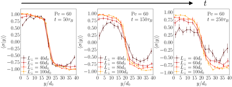
Figure 8: The charge density profiles with different $S$ near the interface at $t=25\tau_{B},75\tau_{B},125\tau_{B}$ for $\text{Pe}=60$ with $L_{\parallel}=100d_{0}$.

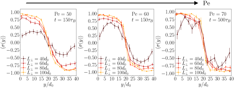
Figure 9: The charge density profiles with different $S$ near the interface varying Pe with $L_{\parallel}=100d_{0}$.

– Interface Mixing at Different Box Shapes

We explain in the main text that TJCs form at the interface between demixed red and blue domains, which causes the demixed state to break down in large systems. As additional supporting evidence for this mechanism, we simulated systems with different aspect ratios: $L_{\parallel}=100d_{0}$ and $L_{\perp}=40d_{0},60d_{0},80d_{0},100d_{0}$ at $\text{Pe}=50,60,70$. This is the regime where diffusive mixing does not apply, and TJCs are playing an important role.

In Fig. 8 we show the time-evolution of the interface profile at $\text{Pe}=60$ and the mechanism described is consistent at different time steps. Each interface profile is averaged over at least 20 simulations and the error bar for the density profile is taken to be the standard error of the average.

The mixing effect depends very weakly on $L_{\perp}$, except for the smallest value ($L_{\perp}=40d_{0}$) which is small enough that a single TJC can affect the whole domain, and is no longer localised near an interface. For the larger systems, this indicates that the mixing can be interpreted as an instability of a single red/blue interface, initiated by a TJC.

In Fig. 9 we show snapshots of the interface profile at $\text{Pe}=50,60,70$: the mechanism consistently observed across this range.

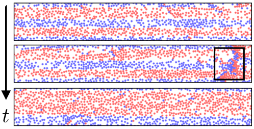
Figure 10: Time series, highlighting a TJC cause coarsening of two lanes. We show a subsystem from large simulation with $L_{\parallel}=150d_{0}$ and ${\rm Pe}=80$.

– Coarsening through TJCs

We have focussed so far on mixing induced by TJCs, starting from a fully demixed state through the creation of the TJCs. Fig. 10 shows an example where this process operate in reverse: the presence of the TJCs disrupts the existing order in the system and causes multiple lanes to merge. (This effect is limited to small systems for which the demixed state is stable.)

References

- Couzin et al. [2003] I. D. Couzin, J. Krause, et al., Advances in the Study of Behavior 32, 10 (2003).
- Ballerini et al. [2008] M. Ballerini, N. Cabibbo, R. Candelier, A. Cavagna, E. Cisbani, I. Giardina, A. Orlandi, G. Parisi, A. Procaccini, M. Viale, et al., Animal behaviour 76, 201 (2008).
- Bialek et al. [2012] W. Bialek, A. Cavagna, I. Giardina, T. Mora, E. Silvestri, M. Viale, and A. M. Walczak, Proceedings of the National Academy of Sciences 109, 4786 (2012).
- Sanchez et al. [2012] T. Sanchez, D. T. Chen, S. J. DeCamp, M. Heymann, and Z. Dogic, Nature 491, 431 (2012).
- Doostmohammadi et al. [2018] A. Doostmohammadi, J. Ignés-Mullol, J. M. Yeomans, and F. Sagués, Nature communications 9, 3246 (2018).
- Tailleur and Cates [2008] J. Tailleur and M. Cates, Physical review letters 100, 218103 (2008).
- Thompson et al. [2011] A. G. Thompson, J. Tailleur, M. E. Cates, and R. A. Blythe, Journal of Statistical Mechanics: Theory and Experiment 2011, P02029 (2011).
- Cates and Tailleur [2015] M. E. Cates and J. Tailleur, Annu. Rev. Condens. Matter Phys. 6, 219 (2015).
- Turing [1952] A. M. Turing, Philosophical Transactions of the Royal Society of London. Series B, Biological Sciences 237, 37 (1952).
- Gray and Scott [1983] P. Gray and S. Scott, Chemical Engineering Science 38, 29 (1983).
- Burger et al. [2016] M. Burger, S. Hittmeir, H. Ranetbauer, and M.-T. Wolfram, SIAM Journal on Mathematical Analysis 48, 981 (2016).
- Dzubiella et al. [2002] J. Dzubiella, G. Hoffmann, and H. Löwen, Physical Review E 65, 021402 (2002).
- Leunissen et al. [2005] M. E. Leunissen, C. G. Christova, A.-P. Hynninen, C. P. Royall, A. I. Campbell, A. Imhof, M. Dijkstra, R. Van Roij, and A. Van Blaaderen, Nature 437, 235 (2005).
- Vissers et al. [2011a] T. Vissers, A. Wysocki, M. Rex, H. Löwen, C. P. Royall, A. Imhof, and A. van Blaaderen, Soft Matter 7, 2352 (2011a).
- Sütterlin et al. [2009] K. Sütterlin, A. Wysocki, A. Ivlev, C. Räth, H. Thomas, M. Rubin-Zuzic, W. Goedheer, V. Fortov, A. Lipaev, V. Molotkov, et al., Physical review letters 102, 085003 (2009).
- Sutterlin et al. [2009] K. R. Sutterlin, H. M. Thomas, A. V. Ivlev, G. E. Morfill, V. E. Fortov, A. M. Lipaev, V. I. Molotkov, O. F. Petrov, A. Wysocki, and H. Lowen, IEEE Transactions on Plasma Science 38, 861 (2009).
- Du et al. [2012] C. Du, K. Sütterlin, K. Jiang, C. Räth, A. Ivlev, S. Khrapak, M. Schwabe, H. Thomas, V. Fortov, A. Lipaev, et al., New Journal of Physics 14, 073058 (2012).
- Sarma et al. [2020] U. Sarma, S. Baruah, and R. Ganesh, Physics of Plasmas 27, 012106 (2020).
- Kondrat et al. [2014] S. Kondrat, G. Oshanin, A. A. Kornyshev, et al., Nanotechnology 25, 315401 (2014).
- Helbing and Molnar [1995] D. Helbing and P. Molnar, Physical Review E 51, 4282 (1995).
- Isobe et al. [2004] M. Isobe, T. Adachi, and T. Nagatani, Physica A: Statistical Mechanics and its Applications 336, 638 (2004).
- Karamouzas et al. [2014] I. Karamouzas, B. Skinner, and S. J. Guy, Physical review letters 113, 238701 (2014).
- Oliveira et al. [2016] C. L. Oliveira, A. P. Vieira, D. Helbing, J. S. Andrade Jr, and H. J. Herrmann, Physical Review X 6, 011003 (2016).
- Bacik et al. [2023] K. A. Bacik, B. S. Bacik, and T. Rogers, Science 379, 923 (2023).
- Couzin and Franks [2003] I. D. Couzin and N. R. Franks, Proceedings of the Royal Society of London. Series B: Biological Sciences 270, 139 (2003).
- Wysocki and Löwen [2009] A. Wysocki and H. Löwen, Physical Review E 79, 041408 (2009).
- Vissers et al. [2011b] T. Vissers, A. van Blaaderen, and A. Imhof, Physical Review Letters 106, 228303 (2011b).
- Li et al. [2021] B. Li, Y.-L. Wang, G. Shi, Y. Gao, X. Shi, C. E. Woodward, and J. Forsman, ACS Nano 15, 2363 (2021).
- Chakrabarti et al. [2003] J. Chakrabarti, J. Dzubiella, and H. Löwen, EPL (Europhysics Letters) 61, 415 (2003).
- Chakrabarti et al. [2004] J. Chakrabarti, J. Dzubiella, and H. Löwen, Physical Review E 70, 012401 (2004).
- Reichhardt and Reichhardt [2006] C. Reichhardt and C. J. O. Reichhardt, Physical Review E 74, 011403 (2006).
- Klymko et al. [2016] K. Klymko, P. L. Geissler, and S. Whitelam, Physical Review E 94, 022608 (2016).
- Vasilyev et al. [2017] O. A. Vasilyev, O. Bénichou, C. Mejía-Monasterio, E. R. Weeks, and G. Oshanin, Soft Matter 13, 7617 (2017).
- Schimansky-Geier et al. [2021] L. Schimansky-Geier, B. Lindner, S. Milster, and A. B. Neiman, Physical Review E 103, 022113 (2021).
- Yu et al. [2022] H. Yu, K. Thijssen, and R. L. Jack, Phys. Rev. E 106, 024129 (2022).
- Glanz and Löwen [2012] T. Glanz and H. Löwen, Journal of Physics: Condensed Matter 24, 464114 (2012).
- Kohl et al. [2012] M. Kohl, A. V. Ivlev, P. Brandt, G. E. Morfill, and H. Löwen, Journal of Physics: Condensed Matter 24, 464115 (2012).
- Geigenfeind et al. [2020] T. Geigenfeind, D. de las Heras, and M. Schmidt, Communications Physics 3, 1 (2020).
- Farrell et al. [2012] F. D. C. Farrell, M. C. Marchetti, D. Marenduzzo, and J. Tailleur, Phys. Rev. Lett. 108, 248101 (2012).
- Stopper and Roth [2018] D. Stopper and R. Roth, Phys. Rev. E 97, 062602 (2018).
- Del Junco et al. [2018] C. Del Junco, L. Tociu, and S. Vaikuntanathan, Proceedings of the National Academy of Sciences 115, 3569 (2018).
- Anderson et al. [2023] C. Anderson, G. Goldsztein, and A. Fernandez-Nieves, Science Advances 9, eadd0635 (2023).
- Weeks et al. [1971] J. D. Weeks, D. Chandler, and H. C. Andersen, The Journal of chemical physics 54, 5237 (1971).
- Thompson et al. [2022] A. P. Thompson, H. M. Aktulga, R. Berger, D. S. Bolintineanu, W. M. Brown, P. S. Crozier, P. J. in ’t Veld, A. Kohlmeyer, S. G. Moore, T. D. Nguyen, R. Shan, M. J. Stevens, J. Tranchida, C. Trott, and S. J. Plimpton, Comp. Phys. Comm. 271, 108171 (2022).
- Korniss et al. [1995] G. Korniss, B. Schmittmann, and R. Zia, EPL (Europhysics Letters) 32, 49 (1995).
- Korniss et al. [1997] G. Korniss, B. Schmittmann, and R. Zia, Journal of Statistical Physics 86, 721 (1997).
- Démery and Dean [2016] V. Démery and D. S. Dean, Journal of Statistical Mechanics: Theory and Experiment 2016, 023106 (2016).
- Poncet et al. [2017] A. Poncet, O. Bénichou, V. Démery, and G. Oshanin, Physical Review Letters 118, 118002 (2017).
- Frusawa [2022] H. Frusawa, Entropy 24, 500 (2022).
- Hansen and McDonald [2013] J.-P. Hansen and I. R. McDonald, Theory of simple liquids: with applications to soft matter (Academic press, 2013).
- Crooks and Chandler [1997] G. E. Crooks and D. Chandler, Physical Review E 56, 4217 (1997).
- Omar et al. [2021] A. K. Omar, K. Klymko, T. GrandPre, and P. L. Geissler, Physical review letters 126, 188002 (2021).
- Dutta and Chakrabarti [2016] S. Dutta and J. Chakrabarti, EPL (Europhysics Letters) 116, 38001 (2016).
- Dutta and Chakrabarti [2018] S. Dutta and J. Chakrabarti, Soft Matter 14, 4477 (2018).
- Dutta and Chakrabarti [2020] S. Dutta and J. Chakrabarti, Physical Chemistry Chemical Physics 22, 17731 (2020).
- Del Junco and Vaikuntanathan [2019] C. Del Junco and S. Vaikuntanathan, The Journal of Chemical Physics 150, 094708 (2019).
- Dean et al. [2020] D. S. Dean, P. Gersberg, and P. C. Holdsworth, Journal of Statistical Mechanics: Theory and Experiment 2020, 033206 (2020).
- Bouchet et al. [2019] F. Bouchet, J. Rolland, and E. Simonnet, Physical review letters 122, 074502 (2019).
- Helbing et al. [2000] D. Helbing, I. J. Farkas, and T. Vicsek, Physical Review Letters 84, 1240 (2000).
- Wensink and Löwen [2012] H. Wensink and H. Löwen, Journal of Physics: Condensed Matter 24, 464130 (2012).
- Bain and Bartolo [2017] N. Bain and D. Bartolo, Nature communications 8, 15969 (2017).
- Bär et al. [2020] M. Bär, R. Großmann, S. Heidenreich, and F. Peruani, Annual Review of Condensed Matter Physics 11, 441 (2020).
- Berthier et al. [2019] L. Berthier, E. Flenner, and G. Szamel, The Journal of Chemical Physics 150 (2019).
- Keta et al. [2022] Y.-E. Keta, R. L. Jack, and L. Berthier, Physical Review Letters 129, 048002 (2022).