Improving the performance of classical linear algebra iterative methods via hybrid parallelism

Abstract

We propose fork-join and task-based hybrid implementations of four classical linear algebra iterative methods (Jacobi, Gauss–Seidel, conjugate gradient and biconjugate gradient stabilized) on CPUs as well as variations of them. This class of algorithms, that are ubiquitous in computational frameworks, are duly documented and the corresponding source code is made publicly available for reproducibility. Both weak and strong scalability benchmarks are conducted to statistically analyse their relative efficiencies.

The weak scalability results assert the superiority of a task-based hybrid parallelisation over MPI-only and fork-join hybrid implementations. Indeed, the task-based model is able to achieve speedups of up to 25% larger than its MPI-only counterpart depending on the numerical method and the computational resources used. For strong scalability scenarios, hybrid methods based on tasks remain more efficient with moderate computational resources where data locality does not play an important role. Fork-join hybridisation often yields mixed results and hence does not seem to bring a competitive advantage over a much simpler MPI approach.

title

[label1]organization=Departament d’Arquitectura de Computadors (DAC), Universitat Politècnica de Catalunya - BarcelonaTech (UPC),addressline=Campus Nord, Edif. D6, C. Jordi Girona 1-3, city=08034 Barcelona, country=Spain

[label2]organization=Barcelona Supercomputing Center (BSC),addressline=Pl. Eusebi Güell 1-3, city=08034 Barcelona, country=Spain

abstract

1 Introduction

Numerical linear algebra plays an important role in the resolution of many scientific and engineering problems. It emerges naturally from the application of the finite difference, finite volume and finite element methods to the numerical resolution of partial differential equations (PDEs) often yielding sparse linear systems. There exist direct and iterative linear algebra methods, being this second class of techniques computationally preferable for large and sparse systems [1]. The first iterative methods were based on relaxation of the coordinates and the ones that remain quite popular even today are the Jacobi and Gauss–Seidel (GS) algorithms. The GS method constitutes an improvement over Jacobi due to its ability to correct the current approximate solution. It is worth mentioning that, in practice, these two techniques are seldom used separately and hence they are often combined (via preconditioning) with more efficient and sophisticated Krylov subspace methods (KSMs). Two great KSM exponents are the conjugate gradient (CG) and the biconjugate gradient stabilized (BiCGStab) methods. The former can be regarded as one of the best-known iterative algorithms for solving sparse symmetric linear systems whilst the latter is made extensible to nonsymmetric linear systems [2]. It is therefore not uncommon to find these four algebraic methods integrated in many numerical libraries and frameworks [3].

The three types of arithmetic operations involved in the aforementioned iterative methods: (i) matrix–vector multiplications, (ii) vector updates, and (iii) scalar products, are well suited for both vector and parallel computers [4]. Matrices and vectors can be efficiently distributed among the processors but the global communication caused, for instance, by the inner product of two vectors represents a major bottleneck on distributed computers. The performance penalty associated with collective communications aggravates with the number of parallel processes and hence can dramatically affect the scalability of iterative methods. This has motivated many researchers to find solutions aimed at reducing the impact of synchronisation barriers present in iterative methods.

In addition to this, parallel implementations of linear algebra methods tend to rely primarily on the message passing interface (MPI) library [5] thus leaving other parallel paradigms and approaches off the table [3, 4]. We are referring to the popular OpenMP fork-join parallelism [6] as well as the less-known task dependency archetype brought by the OmpSs programming model [7] that was first integrated into OpenMP 3.0 in 2008. Having mentioned all that, there exist computational frameworks with support for hybrid parallel programming [8] and also numerical libraries such as PETSc [9], Trilinos [10], or Hypre [11] proposing several levels of parallelism, both hybrid (typically MPI with OpenMP fork-join) and heterogeneous (GPUs). What is more, although task-based hybrid implementations of iterative algebraic methods do exist, e.g. Aliaga et al. [12] or Zhuang and Casas [13], they still remain scarce in the scientific literature and, to the best of our knowledge, are not present in any major computational frameworks. The present study contributes to enhancing the parallel performance of the four aforementioned numerical methods on CPUs by:

• Proposing algorithm variations aimed at reducing or eliminating communication barriers via OpenMP and OmpSs-2 tasks.

• Bringing hybrid parallelism via fork-join and task-based shared-memory programming models in conjunction with MPI.

• Carrying out systematic benchmarks and statistical analysis of the hybrid implementations and comparing them against MPI-only parallel code.

The remainder of this paper is organised as follows. Section 2 presents the related work and Section 3 describes the numerical methods as well as their hybrid implementations. Section 4 contains the main findings of this work and discusses the results in detail. Finally, Section 5 gives the main conclusions and proposes some future work.

2 Related work

Countless examples attempting to improve the parallel efficiency of iterative linear algebra methods can be found in the literature. Skipping over the straightforward Jacobi algorithm, both bicolouring (e.g. a red–black colour scheme) [14] and multicolouring [15] techniques have been proposed for providing independence and therefore some degree of parallelism to the Gauss–Seidel algorithm. However, the appropriateness of such colouring schemes largely depends on the coefficient matrix associated with the linear system. What is more, in order to prevent parallelisation difficulties, processor- and thread-localised GS methods are often employed instead of a true GS parallel method able to maintain the exact same convergence rate of the sequential algorithm [16].

As for Krylov subspace methods, one of the most common improvements consists of reducing the number of global reductions associated with the calculation of the inner product of two vectors. An earlier example applied to the CG algorithm can be found in the book of Barrett et al. [17]. Other authors have successfully reduced the total number of global scalar products to just one via $s$-step methods [18]. One of the main drawbacks of this approach is that numerical issues start arising for increasing orthogonal directions represented by $s$. Other alternatives seek to overlap computational kernels with communication: the pipelined versions suggested by Ghysels and Vanroose [19] result in an asynchronous preconditioned CG algorithm where one of global reductions is overlapped with the sparse matrix–vector multiplication (SpMV) kernel and the other takes advantage of the preconditioning step to hide its communication latency. A more contemporary approach with the name of “iteration-fusing” attempts to partially overlap iterations by postponing the update of the solution residual at the end of each iteration [13]. The main disadvantage of this method is to determine how often to check for the residual as it requires an exhaustive search and remains problem-specific. Needless to say, all the aforementioned works only exploit parallelism via MPI with the exception of the iteration-fusing variant of Zhuang and Casas [13], which heavily relies upon OpenMP tasking to achieve overlapping. This method has been recently improved [20] by intertwining computation and communication tasks using the OmpSs-2 task-based programming model and the task-aware MPI (TAMPI) library [21].

The BiCGStab method has also received a lot of attention. For instance, the MBiCGStab variant proposed by Jacques et al. [22] reduced the three original global synchronisations to only two. Based on the same concept, the nonpreconditioned BiCGStab was improved by Yang and Brent [23] with a single global communication that could be effectively overlapped with computation. Other authors have proposed reordered and pipelined BiCGStab methods, all of them taking advantage of the preconditioning step to hide the communication latency. It is worth noting that, although these variants do not change the numerical stability of the method, they do incur an extra number of computations (due to the increasing role of vector operations) with respect to the classical algorithm. Consequently, there is a trade-off between communication latency and extra computation and therefore it becomes tricky to determine a priori the suitability of each method over the classical BiCGStab algorithm, as demonstrated by Krasnopolsky [24]. What is more, such a comparison will depend on whether parallelisation relies exclusively on the MPI distributed-memory model as in [24] or it is combined with shared-memory parallelism.

To the best of our knowledge, there are not bibliographic references with an extensive comparison of several algebraic methods following pure and hybrid MPI parallelisation strategies using OpenMP and/or OmpSs-2 tasks. To this end, the present study sheds light on the potential gains that hybrid applications can achieve. At the same time, this work is also intended as a reference for effective hybrid programming and code implementation that future researchers can adopt when developing highly scalable numerical methods for linear algebra.

3 Numerical methods and parallel implementations

This section describes all the numerical methods presented in this work as well as their hybrid, parallel implementations currently based on a combination of MPI with OpenMP and OmpSs-2.

3.1 Description of the algorithms

We are particularly interested in bringing hybrid parallelism to linear algebra iterative methods for the numerical resolution of systems of equations of the form ${\bf A}\cdot{\bf x}={\bf b}$, where ${\bf A}$ represents a known sparse matrix, ${\bf b}$ is a known array, and ${\bf x}$ refers to an unknown vector satisfying the equality. Such sparse linear systems typically arise from the numerical approximation of PDEs related to engineering problems like those found in computational fluid dynamics (CFD). We place special emphasis on the OpenFOAM library [3]. This open-source CFD framework provides an extensive range of features to solve complex fluid flows and, because it remains free to use, has a large user base across most areas of engineering and science, from both commercial and academic organisations. We have identified within this CFD library the four most commonly used iterative methods worth studying.

There is a plethora of numerical methods that can be applied to the kind of sparse systems described in the previous paragraph. Some of them can even be combined with preconditioning or smoothing techniques, which are not covered in this work. The two most basic methods that we address are the Jacobi method and the symmetric Gauss–Seidel method. The latter applies one forward sweep followed by a backward sweep within the same iteration and can be seen as an improvement of the former since the computation of a given element of the array ${\bf x}$ uses all the elements that have been previously computed in the current iteration. The other two numerical algorithms covered in this work are CG and BiCGStab. These KVMs rely primarily on SpMV calculations and can achieve better convergence rates than Jacobi and Gauss–Seidel [2]. Since these four algorithms remain highly popular, and are extensively used in OpenFOAM, they become great exponents to study different hybrid parallelisation strategies.

1 ${\bf r}_{0}={\bf b}-{\bf A}\cdot{\bf x}_{0}$, ${\bf p}_{0}={\bf r}_{0}$, $\alpha_{0}=\alpha_{{\rm n},0}/\alpha_{{\rm d},0}={\bf r}_{0}\cdot{\bf r}_{0}/(({\bf A}\cdot{\bf p}_{0})\cdot{\bf p}_{0})$ ;

2 for $j=1,2,\ldots$ do

       if $\sqrt{\alpha_{{\rm n},j-1}}<\epsilon$ then break ;

       // Exit loop

       ${\bf r}_{j}={\bf r}_{j-1}-\alpha_{j-1}{\bf A}\cdot{\bf p}_{j-1}$ ;

        // Tk 0

       $\alpha_{{\rm n},j}={\bf r}_{j}\cdot{\bf r}_{j}$ ;

        // Tk 0

       ${\bf A}\cdot{\bf p}_{j}={\bf A}\cdot{\bf r}_{j}+\frac{\alpha_{{\rm n},j}}{\alpha_{{\rm n},j-1}}{\bf A}\cdot{\bf p}_{j-1}$ ;

        // Tk 1 & 2

       ${\bf p}_{j}={\bf r}_{j}+\frac{\alpha_{{\rm n},j}}{\alpha_{{\rm n},j-1}}{\bf p}_{j-1}$ ;

        // Tk 2

       $\alpha_{{\rm d},j}=({\bf A}\cdot{\bf p}_{j})\cdot{\bf p}_{j}$ ;

        // Tk 2

       ${\bf x}_{j}={\bf x}_{j-1}-\frac{\alpha^{2}_{{\rm n},j-1}}{\alpha_{{\rm d},j-1}\cdot\alpha_{{\rm n},j}}({\bf p}_{j}-{\bf r}_{j})$ ;

        // Tk 3

3      

4${\bf x}={\bf x}_{\rm l}-\alpha_{\rm l}{\bf p}_{\rm l}$ ;

Algorithm 1 Conjugate gradient, nonblocking algorithm (CG-NB) with a schematic task implementation (Tk).

In this work, we propose for hybridisation two nonpreconditioned KVMs, namely CG-NB and BiCGStab-B1, described by Algorithms 1 and 2, respectively. On the one hand, the CG-NB method does apply the SpMV kernel on vector ${\bf r}_{j}$ so that the product ${\bf A}\cdot{\bf p}_{j}$ is simply computed as an array update of ${\bf A}\cdot{\bf r}_{j}$ (line 6 of Algorithm 1). This removes the two communication barriers of the original CG algorithm thus rendering it truly nonblocking: note that the collective reduction caused by the dot product (line 5) can be overlapped with the SpMV on ${\bf r}_{j}$ to then proceed with line 6. Although this algorithm is arithmetically equivalent to the classical one, it might converge slightly different.

1 ${\bf r}_{0}={\bf b}-{\bf A}\cdot{\bf x}_{0}$, ${\bf p}_{0}={\bf r}_{0}$, $\beta_{0}=\mathbf{r}_{0}\cdot\mathbf{r}_{0}$, $\mathbf{r}^{\prime}=\mathbf{r}_{0}/\sqrt{\beta_{0}}$, $\alpha_{{\rm n},0}={\bf r}_{0}\cdot{\bf r}^{\prime}$ ;

2 for $j=0,1,\ldots$ do

       $\alpha_{{\rm d},j}=({\bf A}\cdot{\bf p}_{j})\cdot{\bf r}^{\prime}$ ;

        // Tk 0 (blocking)

       ${\bf s}_{j}={\bf r}_{j}-\alpha_{j}{\bf A}\cdot{\bf p}_{j}$ ;

        // Tk 1

       $\omega_{j}=({\bf A}\cdot{\bf s}_{j})\cdot{\bf s}_{j}/(({\bf A}\cdot{\bf s}_{j})\cdot({\bf A}\cdot{\bf s}_{j}))$ ;

        // Tk 2

       ${\bf x}_{j+1/2}={\bf x}_{j}+\alpha_{j}{\bf p}_{j}$ ;

        // Tk 3

       if $\sqrt{\beta_{j}}<\epsilon$ then break ;

       // Exit loop

       ${\bf x}_{j+1}={\bf x}_{j+1/2}+\omega_{j}{\bf s}_{j}$ ;

        // Tk 4

       ${\bf r}_{j+1}={\bf s}_{j}-\omega_{j}{\bf A}\cdot{\bf s}_{j}$ ;

        // Tk 4

       $\alpha_{{\rm n},j+1}={\bf r}_{j+1}\cdot{\bf r}^{\prime}$ ;

        // Tk 4

       $\beta_{j+1}={\bf r}_{j+1}\cdot{\bf r}_{j+1}$ ;

        // Tk 4

       ${\bf p}_{j+1/2}={\bf p}_{j}-\omega_{j}{\bf A}\cdot{\bf p}_{j}$ ;

        // Tk 5

3       if $\sqrt{\alpha_{{\rm n},j+1}}<\varepsilon$ then // Restart procedure

             ${\bf p}_{j+1}={\bf r}_{j+1}$ ;

              // Tk 6

             ${\bf r}^{\prime}={\bf r}_{j+1}/\sqrt{\beta_{j+1}}$ ;

              // Tk 6

4            

5       else // Regular procedure

             ${\bf p}_{j+1}={\bf r}_{j+1}+\frac{\alpha_{{\rm n},j+1}}{\alpha_{{\rm d},j}\cdot\omega_{j}}{\bf p}_{j+1/2}$ ;

              // Tk 7

6            

7      

8${\bf x}={\bf x}_{\rm l}+\omega_{\rm l}{\bf s}_{\rm l}$ ;

Algorithm 2 Biconjugate gradient stabilized, one blocking algorithm (BiCGStab-B1) with a schematic task implementation (Tk).

On the other hand, the BiCGStab-B1 variant permutes the order of certain operations in order to eliminate two of the three barriers present in the original algorithm. It is the dot product associated with $\alpha_{{\rm d},j}$ (line 3 of Algorithm 2) the responsible of such blocking synchronisation. However, the two scalar products, i.e. numerator and denominator of $\omega_{j}$ (line 5), can be overlapped with the update of ${\bf x}_{j+1/2}$ at line 6. Likewise, the scalar products corresponding to $\alpha_{{\rm n},j+1}$ and $\beta_{j+1}$ (lines 10–11) can be overlapped with the update of ${\bf p}_{j+1/2}$ at line 12. It is worth noting that the effective overlapping of these two parts of the BiCGStab-B1 algorithm is only possible if the computation times associated with vector updates remain larger than those of collective communications.

We highlight that the major novelty of Algorithms 1–2 resides in their combination with a task-based programming language that can fully exploit their parallel performance. Note that Algorithms 1–2 showcase the strict minimum number of distinct tasks necessary to fully parallelise them (see r.h.s. comments beginning with keyword Tk): four tasks for the CG-NB algorithm and eight tasks for BiCGStab. In this document, the task notation has been simplified and enumerated for clarity and the reader is referred to [25] for the actual task implementation in full detail.

As it is the case with other strategies from the literature [22, 23], the two proposed methods do incur extra operations. In the case of CG-NB, there is an additional vector update (line 9) which can be optimised via the ad hoc kernel ${\bf z}:=a\cdot{\bf x}+b\cdot{\bf y}+c\cdot{\bf z}$ that reuses memory. Let $r$ and $\bar{n}$ represent the number of rows and the average number of nonzeros per row of the sparse matrix, respectively. A rough estimate of the total number of accessed elements per iteration of the CG-NB algorithm is given by $(15+\bar{n})r$, which is slightly larger than the $(12+\bar{n})r$ corresponding to CG. Applying the same reasoning, one can find the exact same difference of $3r$ elements between the BiCGStab algorithm, $(21+2\bar{n})r$, and the variant proposed here, $(24+2\bar{n})r$. In this work, we consider two sparsity levels: $\bar{n}=7$ and $\bar{n}=27$. The lower value is derived from applying a 7-point centred stencil on a three-dimensional structured hexahedral mesh and is typical of an OpenFOAM application. The higher sparsity level originates from applying a 27-point centred stencil to the same mesh and is actively used by the well-known HPCG benchmark [26]. Therefore, the maximum relative increase of touched elements will be given by $3/(12+\bar{n})\approx 15.8\%$ for CG-NB and $3/(21+2\bar{n})\approx 8.6\%$ for BiCGStab-B1. These figures are on par with other approaches proposed in the past; for example, a similar amount of extra operations is required for the IBiCGStab algorithm proposed by Yang and Brent [23] after aggregating every additional vector update and scalar product into a single, ad hoc function. On the one hand, this improved algorithm of Yang & Brent yields a single, nonblocking synchronisation; on the other hand, it relies upon the transpose of the input matrix and necessitates much more system memory. Likewise, it does not offer support for restarting but, if it were the case, then it would require a third SpMV operation per iteration affecting severely its performance. Restarting not only helps improving numerical convergence, but it is also critical for task-based parallel implementations (see Section 3.3). For the reasons mentioned above, we cannot consider the IBiCGStab algorithm suitable for hybridisation.

3.2 Description of the parallel framework

Even though OpenFOAM already provides a MPI parallel implementation of the classical versions of the methods described in the previous section, it is not used here as a reference framework due to its tremendously large code base. Instead, we implement our numerical codes within the HPCCG benchmark [27]. This application is a minimalist version of the famous HPCG benchmark [26] used in the TOP500 supercomputer list and was developed by the same authors in the context of the Mantevo project [28]. HPCCG applies the classical CG on a sparse system encoded in the popular compressed sparse row (CSR) matrix format. Similarly to OpenFOAM, HPCCG only supports distributed parallelism via MPI (MPI-only).

We provide two approaches to hybrid parallelism, one using the fork-join paradigm with the clause parallel for from OpenMP (MPI-OMP_fj) and the other based on tasks via either OpenMP (MPI-OMP_t) or OmpSs-2 (MPI-OSS_t). The most significant difference between these two approaches resides in the fact that, when programming using the OpenMP fork-join model, the developer needs to identify which regions of the program will be executed in parallel. Nevertheless, the overlapping of computation and communication phases can become challenging. On the other hand, in the OmpSs-2 tasking model, the parallelism is implicitly created from the beginning of the execution. As a consequence, the developer needs to identify the tasks that will be executed asynchronously and their input/output dependencies to leverage its data-flow execution model. The tasking model requires more effort from the programmer but enables the transparent overlapping of computation and communication phases with the help of the TAMPI library [7, 21].

Finally, all the extensions that we made to the HPCCG open-source code have been published at Code Ocean [25] under the name HLAM (hybrid linear algebra methods) to make them available to future readers. The next two sections describe the hybrid implementations of the CG-NB and the relaxed, symmetric Gauss–Seidel methods within HLAM. The other algorithms undergo a similar procedure and, for the sake of conciseness, are omitted in this work.

3.3 Parallelisation of the CG-NB algorithm

We follow the HDOT strategy that we recently published [29] with the aim of facilitating the programming of hybrid, task-based applications. We define “domains” as the result of applying an MPI explicit decomposition: a spatial grid in this particular case. It is explicit in the sense that the programmer needs to design the application from scratch with a very specific decomposition that is quite difficult to modify afterwards because it requires major code refactoring. Next, HDOT defines a deeper hierarchy of “subdomains” to which one can assign individual tasks that can be executed in parallel via appropriate OpenMP or OmpSs-2 clauses with their corresponding read (in) and write (out) data dependencies. This introduces minimal refactoring in MPI-only applications such as HPCCG thus leaving the original MPI decomposition intact. Finally, in order to intertwine the two parallel programming models, e.g. MPI-OMP and MPI-OSS, the communication tasks rely upon the TAMPI library [21] which permits to overlap them with other computation tasks transparently to the programmer. It is worth mentioning that the HDOT strategy targets truly hybrid applications with zero sequential parts and zero implicit (fork-join) barriers. Hence, we expect such hybrid applications to outperform their MPI-only counterparts in most scenarios.

Code 1 shows two intermediate tasks (Tk 1 and Tk 2 as described by Algorithm 1) inside the main loop of the CG-NB method as well as the point-to-point MPI communication of vector ${\bf r}$ (line 1) before the SpMV (line 12) and the collective communication of $\alpha_{d}$ (line 24). In order to assign tasks to subdomains it is necessary to divide the iterative space, that is nrow, which represents the actual length of the involved arrays after the explicit decomposition of MPI. This is done with an external loop (line 6) and appropriate starting indexes and block sizes (line 7). The total number of tasks is provided by the user at runtime and determines the granularity. As a rule of thumb, there should be enough tasks to feed all the cores; however, having too many of them will cause overheads and ultimately impact the parallel performance. Moving forward, the task computing the SpMV (lines 9–12 in Code 1) needs a multidata read dependency on ${\bf r}$ and a regular write dependency on a region of Ar that stores the sparse matrix–vector product ${\bf A}\cdot{\bf r}$ (line 11). Indeed, the SpMV kernel has the particularity of accessing noncontiguous elements of r thus yielding an irregular data access pattern, which we precalculate and store in variables depMVidx and depMVsize at the beginning of the program for later reuse. The next task (lines 14–21) performs altogether two vector updates and one scalar product using regular data dependencies. It is worth mentioning the use of the macro ISODD, which allows us to carry out independent MPI communications along two consecutive iterations by exploiting different communicators. In practice, this prevents any possibility of MPI deadlocks associated with different iterations of the main loop.

Special attention must be paid to local reductions via tasks when calculating, for instance, $\alpha_{\rm d}$ at line 21 of Code 1. Contrarily to the MPI-only or MPI-OMP_fj implementations, the task execution order is not guaranteed between consecutive iterations or two complete executions of the CG-NB algorithm. As a result, floating-point rounding errors can accumulate and affect the convergence rate of the entire algorithm. Whilst this does not constitute an issue for the CG methods, it does have devastating consequences for the BiCGStab algorithm and its derivatives. It is well known that BiCGStab is prone to divergence when the residual $\sqrt{\alpha_{n,j+1}}$ (see line 10 of Algorithm 2) gets closer to zero. Tasks do aggravate this situation and, as a result, each BiCGStab execution is susceptible to reaching convergence a handful number of iterations later (convergence is typically attained after a few tenths of iterations or less). To prevent this from happening, we employ a restart procedure (lines 13–15 of Algorithm 2) that triggers whenever the residual value reaches a given threshold (typically $\varepsilon=10^{-5}$, although it may be problem-specific and require additional tunning). Restarting not only reduces the total number of iterations to reach convergence for all the parallel implementations tested in this work, but it also eliminates the accumulative rounding errors introduced by the task execution order. Note, however, that this nondeterministic execution order may not be desirable for high fidelity simulations where instantaneous fields need to be accurately reproduced.

The function exchange_externals performing the point-to-point communication is shown in Code 2. Neighbouring data is received close to the end of buffer x (line 8) to later be used by the SpMV kernel. As for sending data, it is a bit more complicated due to the irregular access pattern caused by the explicit MPI decomposition. Therefore, the use of multidata dependencies becomes necessary again. Note that in one single task data are copied, arranged contiguously in a temporary buffer, and sent to the corresponding neighbour. These two communication tasks (lines 6–9 and 17–23) are transparently scheduled and executed along with computation tasks with the aid of the TAMPI library. The TAMPI_IWAIT specialised nonblocking function converts the MPI synchronicity into a regular task data dependency handled automatically by the OmpSs-2 runtime (the same holds true with OpenMP tasks and the OpenMP runtime).

Hybrid parallelism can also be achieved by combining MPI with OpenMP and its fork-join model, which today constitutes the most common archetype of hybrid programming. Code 3 shows how this model is supported in the SpMV function in such a way that still remains compatible with the task-based implementation described above. Within each subdomain of length size, the iteration space is further subdivided in blocks of size bs and assigned to different OpenMP threads, see lines 1–11. In practice, however, when the fork-join model is enabled the number of subdomains is reduced to one as there are no tasks present. The same strategy is adopted in other functions (axpby, dot, etc.). The amount of work distributed to each thread is carried out by the function split at line 2 of Code 3. This subroutine attempts to align partitions to boundaries compatible with the specified SIMD vector length whenever possible (see lines 16–17). This function is also employed to determine the best number of subdomains (tasks) while seeking optimal vectorisation properties. As it is the case when using, for example, Intel MKL parallel functions, fork-join parallelism remains internal to the kernel and, therefore, switching from one kernel to another yields an implicit barrier that is not present in the task-based implementation (although the use of nowait clauses may help in eliminating such barriers). Finally, this fork-join implementation cannot handle MPI collectives via tasks and, therefore, it reuses MPI synchronous calls (MPI_Wait and MPI_Allreduce) originally implemented in HPCCG.

3.4 Parallelisation of the relaxed Gauss–Seidel algorithm

In the particular case of the symmetric Gauss–Seidel solver, the most adopted task-based strategy consists of assigning colours to subdomains or tasks. This brings new opportunities for parallelisation by assuming that each colour can be calculated independently so that data dependencies only affect tasks belonging to the same colour. However, this assumption does not guarantee the exact same execution order of the original algorithm, which is essentially sequential. As a result, the parallel algorithm can exhibit a different convergence behaviour. Our standard task-based parallelisation of the GS algorithm supports multicolouring and colour rotation between iterations but, for practical reasons, a red–black colour scheme without rotation is adopted herein. Indeed, for the sparse matrices used in this work, this basic strategy gives us the best performance and no further advantages are observed with the addition of more colours. This can be explained by the fact that both HLAM and HPCCG codes work on structured meshes.

We decide to go one step further in the parallelisation of the GS method by assigning a new set of task clauses that do not complain with the red–black colouring scheme but, on the other hand, do reduce the complexity of task data dependencies. Code 4 shows the computation tasks inside the main loop of this relaxed implementation. The forward and backward sweeps contain a regular write dependency on vector ${\bf x}$ instead of the expected multidependency that is present in the bicoloured task-based implementation. Each sweep is self-contained in a different loop (lines 8–12 and 15–20) to guarantee that tasks associated with forward sweeps over a particular subdomain are computed before the backward sweep. We introduce an extra level of task synchronicity when initialising the local residual at lines 1–6. This is to avoid any computation overlaps between different iterations. The task annotation shown in Code 4 guarantees numerical convergence because the data races that are created mimic the Gauss–Seidel behaviour in which previously calculated data are being continuously reused within the current iteration. Not having data races will imply a slowdown in convergence for this relaxed implementation, making it similar to that of the Jacobi method.

4 Results and discussion

This section evaluates the CG, BiCGStab, symmetric Gauss–Seidel and Jacobi original methods as well as the proposed alternative versions. Similarly, different parallelisation strategies are compared against each other and analysed in detail.

4.1 Numerical setup

We carry out the numerical experiments on the MareNostrum 4 supercomputer, located at the Barcelona Supercomputer Center (BSC). Each computational node is equipped with two Intel Xeon Platinum 8160 CPUs composed of 24 physical cores (hyperthreading disabled) running at a fixed frequency of $\mathrm{2.1\,GHz}$. The L3 cache memory of this CPU is $\mathrm{33\,MiB}$. We pay special attention to this number and verify that our memory-bound applications are actually limited by the system main memory (RAM). To ensure this, each process of a MPI-only application works on a grid size of $128\times 128\times 128$ elements and, in the case of a hybrid application (1 MPI process per socket), this quantity is increased by a factor of 24 ($128\times 128\times 3072$, note that HPCCG, and thus HLAM, only distribute points along the last dimension). This implies 384 MiB per array (stored in double precision), which is one order of magnitude larger than the L3 cache. For a fair comparison between different methods and parallel implementations, results presented in the same graph are run within the same job script, thus using the exact same computational resources, and repeated up to ten times in order to extract relevant statistics. A version of Clang 15 modified by BSC constitutes the predetermined compiler: it allows us to quickly switch between OpenMP and OmpSs-2 runtimes. The source code is compiled with the usual flags -march=native and -Ofast together with support for 512-bit SIMD vector instructions and memory alignment to 2 MiB transparent huge pages. Finally, Intel’s MPI library 2018.4 is used for all the experiments carried out on MareNostrum 4.

The sparse linear system to be solved is the standard one proposed by the HPCG benchmark [26] and arises from the finite discretisation of a centred stencil on a three-dimensional hexahedral mesh. The r.h.s. vector $\mathbf{b}$ is defined analytically for the exact solution $\mathbf{x=1}$. Next, the numerical method is initialised to $\mathbf{x=0}$ and is let to evolve with the convergence criteria set to $\epsilon=10^{-6}$ together with a restarting threshold value of $\varepsilon=10^{-5}$ for the BiCGStab methods. The required number of iterations to reach convergence depends strongly on the numerical method and the degree of sparsity of the system matrix and, to a much lesser extent, the parallel implementation. When using one compute node of MareNostrum 4 and the 7-point centred stencil, the required iterations are: 8 (BiCGStab), 12 (CG), 9 (Gauss–Seidel), and 18 (Jacobi); similarly, the iterations associated with the 27-point stencil are: 45 (BiCGStab), 72 (CG), 142 (Gauss–Seidel), and 515 (Jacobi).

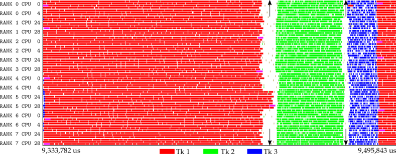
(a) CG algorithm

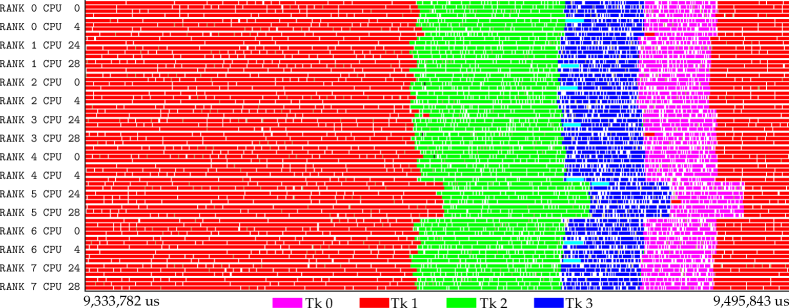
(b) CG-NB algorithm

Figure 1: Paraver traces associated with the (a) classical CG and (b) nonblocking CG (CG-NB) hybrid methods implemented via MPI-OSS_t using 8 MPI ranks and 8 cores per rank. Events highlighted in different colours correspond to OmpSs-2 tasks. Arrows indicate blocking barriers due to MPI collective communication.

4.2 Weak scalability of Krylov subspace methods

We compare the CG and BiCGStab methods using several parallelisation strategies. For task-based implementations, we first need to identify the optimal task granularity, which mainly depends on the task dependency graph associated with the SpMV operation. This process, omitted here for the sake of conciseness, can be automated by executing the application binary with an increasing number of tasks multiple of the available resources (24 cores per socket on MareNostrum 4). The optimal task granularity turns out to be around 800 tasks and 1500 tasks depending on the matrix sparsity pattern, that is 7- and 27-point stencils, respectively. It is worth mentioning that there is a fair interval around these numbers where the performance still remains optimal. The granularity is mainly determined by the most computationally intensive kernel, i.e. SpMV, and for this reason the optimal granularity is quite similar among different Krylov methods. The same applies to the Jacobi and symmetric Gauss–Seidel methods, where the algorithm access pattern resembles quite a lot that of the SpMV with additional operations over the diagonal elements of the matrix.

Before comparing different methods and implementations against each other, it is worth discussing the improvements brought by the proposed algorithms. Figure 1 shows two Paraver traces corresponding to the original and nonblocking CG methods. They are obtained after executing the respective hybrid implementations making use of MPI and OmpSs-2 tasks under the exact same computational resources: 8 MPI ranks and 8 cores per rank in order to improve the readability of the trace. The time interval, which is the same for both traces, is sufficiently large to cover one entire loop iteration approximately. For the classical version, Fig. 1(a), the presence of two synchronisation barriers (indicated by arrows) due to collective MPI communication is evident. For the nonblocking method, Fig. 1(b), coloured events correspond to different tasks as described in Algorithm 1. The same labels and colours have been retained on both figures although there is not a straight one-to-one mapping of tasks between these two methods. From the results shown above, it can be stated that the proposed CG-NB algorithm, when executed via the MPI-OSS_t hybrid model, can effectively suppress the two blocking barriers present in the original method. The same can be said for the BiCGStab-B1 method, where the hybrid implementation based on tasks does eliminate two of the three global barriers. We purposely omit the corresponding traces for the sake of brevity.

Time [s]

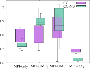
(a) CGs, 7-pt stencil

Time [s]

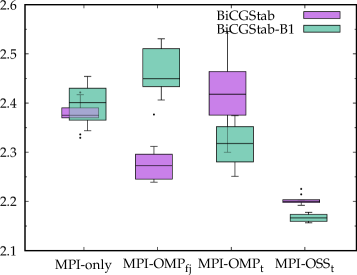
(b) BiCGStabs, 7-pt stencil

Figure 2: Execution time comparison between several parallel implementations of the classical and the proposed variants of the (a) CG and (b) BiCGStab methods on 16 compute nodes of MareNostrum 4 using the 7-point stencil pattern. Standard box and whisker plots.

The objective of Figs. 2(a)–(b) (box and whisker plots) is to show the execution time variability of various parallel implementations of KVMs using 16 compute nodes and the sparsest coefficient matrix associated with a 7-point spatial stencil. Starting with the classical CG version, Fig. 2(a), the MPI-only implementation and the two hybrid ones based on OpenMP report similar median times with significant variations between executions. On the other hand, the task-based OmpSs-2 implementation yields a significant improvement, both in terms of execution time and variability, being the median execution time 7.7% lower with respect to the MPI-only implementation. When switching to the nonblocking CG method, MPI-OMP_fj and MPI-OMP_t versions do report larger times due to the extra number of memory accesses (see Section 3.1); to our surprise, this is not the case for the MPI-only implementation. The nonblocking, OmpSs-2 version shows an additional improvement of 4% over its classical counterpart. Moving on to the original BiCGStab method, see Fig. 2(b), the OpenMP fork-join and OmpSs-2 task-based implementations offer speedups of 4.5% and 12% over the MPI-only version, respectively. The task-based implementations of the BiCGStab-B1 algorithm can suppress two of the three synchronous points per iteration by overlapping computation with communication tasks via the TAMPI library. This leads to relative improvements of 4.3% and 1.5% for the OpenMP and OmpSs-2 runtimes, respectively. As expected, they remain rather modest compared to those seen for CG since there still remains one unavoidable synchronisation at line 3 of Algorithm 2. Finally, it is worth noting the remarkable reduction in execution variability achieved by the tight integration of MPI and OmpSs-2 programming models via the TAMPI library. The remainder of this work focuses on the OmpSs-2 task-based version due to its superiority over OpenMP tasks and evaluates both the weak and strong scalabilities of four algorithms and three parallel implementations over a broad range of compute nodes using two sparsity degrees for the coefficient matrix.

Figure 3 shows the results derived from a weak scalability analysis of the CG and BiCGStab methods using several parallel implementations and sparsity patterns. To facilitate the comparison, times will always be normalised by the MPI-only, classical version of each algorithm executed on one compute node, which assigns the value of 1 to the first filled square point of each graph. Consequently, these figures do report relative parallel efficiencies and, for this reason, some values may exceed unity. Absolute execution time values can be easily retrieved from graphs with the specified reference times. Beginning with the classical CG methods, Figs. 3(a)-(b), the OmpSs-2 version turns out to be overall much faster than its MPI-only counterpart except when employing one node and the 7-point stencil. By switching from the classical algorithm to the nonblocking one, this task-based implementation becomes 19.7% and 25% faster than the MPI-only version for the 7- and 27-point stencils, respectively, when using 64 compute nodes. The fork-join hybrid implementation yields mixed results, being only faster than the MPI-only version when considering the 27-point stencil. As it was the case of Fig. 2, the proposed nonblocking algorithm only benefits the MPI-only and task-based versions and is counterproductive with fork-join parallelism. Regarding the BiCGStab methods, Figs. 3(c)-(d), results are generally similar to those observed for CG with minor discrepancies. For instance, only the task-based implementations take advantage of the BiCGStab-B1 algorithm by a small, but consistent margin. Therefore, they remain faster than the classical algorithm by 1.4% and 0.7% for the 7- and 27-point stencils, respectively, when using the largest set of compute nodes. As previously mentioned, such small percentages are expected because of the remaining global barrier. For this same node configuration, the BiCGStab task-based version is, depending on the sparsity pattern, 10.6% and 20% faster than the MPI-only classical implementation and overall more efficient than the fork-join hybrid version.

Relative parallel eff. [–]
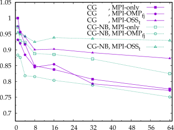
	Compute nodes [–]

(a) CGs, 7-pt stencil

Relative parallel eff. [–]
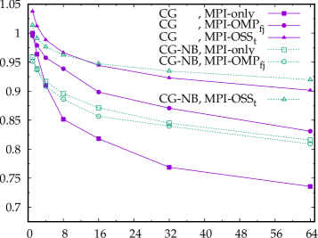
	Compute nodes [–]

(b) CGs, 27-pt stencil

Relative parallel eff. [–]
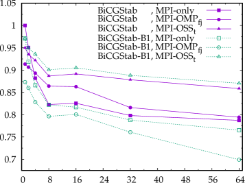
	Compute nodes [–]

(c) BiCGStabs, 7-pt stencil

Relative parallel eff. [–]
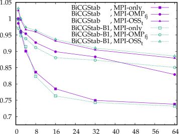
	Compute nodes [–]

(d) BiCGStabs, 27-pt stencil

Figure 3: Relative parallel efficiencies associated with the weak scalability analysis of the CG and BiCGStab methods with two sparsity patterns using up to 64 compute nodes of MareNostrum 4. Median reference times correspond to the MPI-only, classical implementations on one compute node (first filled square): (a) 1.52s, (b) 19.35s, (c) 1.96s and (d) 23.76s. Each point represents the median value of 10 executions.

Another aspect worth mentioning about Fig. 3 is the fact that the MPI-only implementations of the CG and BiCGStab methods do not seem to benefit from the increase in computational intensity caused by the 27-point stencil. Indeed, the relative parallel efficiencies are equal or worse than those obtained with the 7-point stencil, contrarily to what the shared-memory strategies report. In any case, we do not expect large discrepancies when switching stencils since the problem size is large enough to guarantee that each kernel within the application remains memory bound.

A final note must be added with regard to the quick degradation of MPI-only implementations with an increasing number of compute nodes. For instance, Fig. 3(a) reveals that the relative parallel efficiency of the CG method drops 15% with eight compute nodes (384 MPI processes). Such a loss in performance is mostly related to the computation of the two dot products and, more specifically, to the corresponding global reductions due to the increasing number of internode communications. Although MPI_Allreduce synthetic benchmarks report typical latencies within the order of $\mathrm{10^{-5}\,s}$ for small message sizes on MareNostrum 4, we can measure latencies of about $\mathrm{10^{-3}\,s}$ on average for the CG method. The two MPI collective communications shown in Fig. 1(a) are good examples of these time intervals. Contrarily to a synthetic benchmark, a complex application like CG is more sensitive to system load imbalances and noise affecting computations between two consecutive collectives. As a result, the effective communication time spent in global communications can be up to two orders of magnitude larger than the minimum latency retrieved from a simple benchmark. These overheads accumulate iteration after iteration and add up to the total execution time. MPI-only applications tend to suffer more from load-balancing issues and this situation aggravates with the increasing core count of new CPUs.

Relative parallel eff. [–]
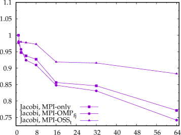
	Compute nodes [–]

(a) Jacobis, 7-pt stencil

Relative parallel eff. [–]
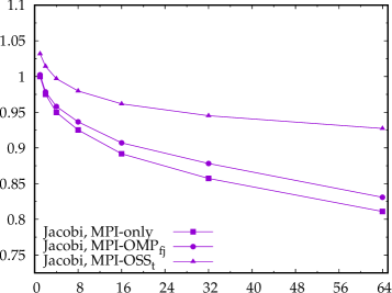
	Compute nodes [–]

(b) Jacobis, 27-pt stencil

Relative parallel eff. [–]
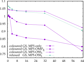
	Compute nodes [–]

(c) Gauss–Seidels, 7-pt stencil

Relative parallel eff. [–]
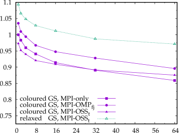
	Compute nodes [–]

(d) Gauss–Seidels, 27-pt stencil

Figure 4: Relative parallel efficiencies associated with the weak scalability analysis of the Jacobi and symmetric Gauss–Seidel methods with two sparsity patterns using up to 64 compute nodes of MareNostrum 4. Median reference times correspond to the MPI-only reference implementations on one compute node (first filled square): (a) 1.40s, (b) 113.91s, (c) 1.31s and (d) 61.65s. Each point represents the median value of 10 executions.

4.3 Weak scalability of Jacobi and symmetric Gauss-Seidel methods

We carry out the same scalability study for the Jacobi and symmetric Gauss–Seidel methods and report the relative parallel efficiencies in Fig. 4. A similar legend and nondimensionalisation of results are employed to help facilitating the comparison with previous Krylov methods. Jacobi is the most straightforward algorithm and one unique kernel is written using three different parallel implementations. While the MPI-only and MPI-OMP_fj methods do report more or less similar execution times, see Figs. 4(a)-(b), the MPI-OSS_t is able to bring more performance to the table. With 64 compute nodes, MPI-OSS_t offers a 14.4% and 14.3% speedup over the MPI-only version employing the 7- and 27-point stencils, respectively. In the case of the symmetric Gauss–Seidel algorithm, we show the typical task-coloured implementation as well as the data-relaxed version implemented with tasks and compare them against the MPI-only and fork-join hybrid alternatives. On the one hand, the fork-join approach seems to have a competitive advantage over pure MPI with the exception of the last point of Fig. 4(c). On the other hand, the two task-based implementations can behave quite differently. When using the sparsest matrix, the red–black colouring strategy can offer a competitive advantage on large core counts, but not for a large margin. However, when the matrix becomes less sparse, Fig. 4(d), the task-based approach based on two colours may result in terrible performance. Contrarily, the relaxed version excels in this particular case. These remarkable differences in efficiency can be easily explained by the number of iterations that each parallel implementation of the GS necessitates to reach numerical convergence. While the MPI-only version convergences in 157 iterations, the bicoloured task-based GS needs 166 and the relaxed version finishes at 150; for reference, the fork-join implementation takes 152 iterations. One can reduce this number of iterations of the coloured version by simply coarsening the task granularity. However, we do not recommend this strategy since combining the symmetric Gauss–Seidel method as a preconditioner with a Krylov algorithm, and using different granularities for each technique, will certainly derive in bottlenecks. Finally, taking into account the best task-based GS implementation on 64 nodes, the obtained speedups are 15.9% and 13.1% with respect to the MPI-only version using the 7- and 27-point stencils, respectively.

4.4 Strong scalability of hybrid iterative methods

The last battery of results correspond to strong scalability tests in which the problem size of $128\times 128\times 6144$ elements does not longer increase with the number of computational resources. In order to avoid excessive repetition, for each parallel implementation we only consider the overall best performing algorithm: classical or proposed variant. Regarding task-based hybrid implementations, we use the optimal task granularity, which we calculate in advance. For convenience, the next figures make use of the same legend and nondimensionalisation specified for the weak scalability graphs.

Relative parallel eff. [–]
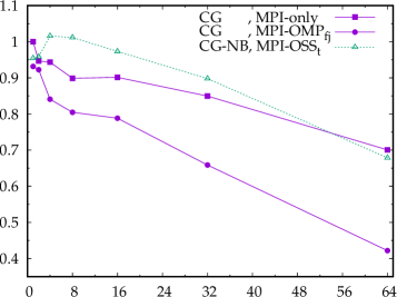
	Compute nodes [–]

(a) CGs, 7-pt stencil

Relative parallel eff. [–]
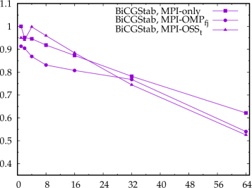
	Compute nodes [–]

(b) BiCGStabs, 7-pt stencil

Relative parallel eff. [–]
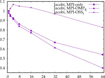
	Compute nodes [–]

(c) Jacobis, 7-pt stencil

Relative parallel eff. [–]
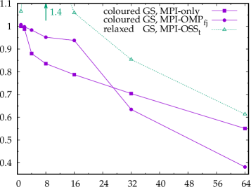
	Compute nodes [–]

(d) Gauss–Seidels, 7-pt stencil

Figure 5: Relative parallel efficiencies associated with the strong scalability analysis of four iterative methods using the 7-point stencil pattern. Same legend and nondimensionalisation as in Figs. 3(a),(c) and Figs. 4(a),(c).

Figure 5 shows the strong scalability results of the four iterative methods considered in this work using the sparsest matrix derived from a 7-point stencil. As expected, when the problem size begins to fit within the L3 cache, the computational advantage of tasks vanishes due to data locality issues. In such scenarios, either the pure MPI approach or the fork-join implementation will exploit data locality better. As the number of computational resources keeps growing, MPI-OSS_t implementations of the two KVM methods, Figs. 5(a)-(b), report quite similar or even subpar performances with respect to their corresponding MPI-only versions. The iterative methods of Jacobi and, in particular, the relaxed Gauss–Seidel do exhibit superscalability when executed via OmpSs-2 tasks, see Figs. 5(c)-(d). In general, the fork-join hybrid implementations do not seem to represent a real improvement over MPI-only and often result in the slowest parallel implementation. Finally, note that the proposed BiCGStab-B1 method is not shown in Fig. 5(b) since it yields overall worse results than the classical algorithm for strong scalability scenarios. The same situation is observed when using the less sparse matrix derived from the 27-point spatial stencil.

Relative parallel eff. [–]
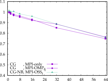
	Compute nodes [–]

(a) CGs, 27-pt stencil

Relative parallel eff. [–]
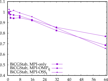
	Compute nodes [–]

(b) BiCGStabs, 27-pt stencil

Relative parallel eff. [–]
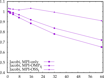
	Compute nodes [–]

(c) Jacobis, 27-pt stencil

Relative parallel eff. [–]
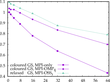
	Compute nodes [–]

(d) Gauss–Seidels, 27-pt stencil

Figure 6: Relative parallel efficiencies associated with the strong scalability analysis of four iterative methods using the 27-point stencil pattern. Same legend and nondimensionalisation as in Figs. 3(b),(d) and Figs. 4(b),(d).

The last results from strong scalability benchmarks carried out with the 27-point stencil are summarised in Figure 6. When looking at the CG and BiCGStab methods, the results are close to those obtained in Fig. 5: the task-based versions start with a competitive advantage that cancels out progressively with the number of computational resources. Nonetheless, the three parallel implementations report similar relative efficiencies and hence there are not remarkable differences between them in terms of execution time, see Figs. 6(a)-(b). The hybrid implementation based on tasks reports the best efficiency figures for the Jacobi and GS methods followed after by the fork-join model. In this particular case, the ubiquitous MPI-only parallelisation is at a clear disadvantage against the two hybrid ones.

5 Conclusions and future work

In this work, we have presented the hybrid implementation on CPUs of four iterative methods, namely: Jacobi, symmetric Gauss–Seidel, conjugate gradient, and biconjugate gradient stabilized. Alternative versions of these algorithms, reducing the number of blocking barriers or completely eliminating them, have also been proposed and compared against the original ones. The hybridisation via OpenMP fork-join parallelism as well as via OpenMP and OmpSs-2 tasks follows the HDOT methodology that we described in a previous paper. Specific code examples are described in detail in this document whilst the entire HLAM source code has been made publicly available at Code Ocean for reproducibility and also to be used as a guide for hybrid programming and code implementation of linear algebra iterative methods.

The weak scalability tests asseverated the superiority of task-based hybrid implementations over the well-known MPI-only and fork-join hybrid implementations. In general, hybrid codes based on the popular OpenMP fork-join paradigm have yielded mixed results, offering sometimes similar or even subpar performance with respect to the MPI-only implementation. The nonblocking alternative versions proposed in this document have also demonstrated to further improve the overall efficiency of the algorithms. The battery of strong scalability benchmarks has shown a competitive advantage of hybrid parallel methods based on tasks for moderate computational resources where data locality effects are not important. While the reported efficiencies remained quite similar for the three parallel implementations of Krylov methods, adding tasks to Jacobi and Gauss–Seidel offered a notorious speedup over MPI-only and MPI-OMP_fj models.

This paper demonstrates the appropriateness of bringing hybrid parallelism, in particular task-based parallelism, into numerical libraries such as OpenFOAM and PETSc, which extensively exploit the numerical methods presented herein. As a future work, we plan to include these hybrid algorithms in a minimalist version of this popular CFD library and report the observed gains. In addition to this, we are planning to continue our code developments over the popular HPCG benchmark, which features preconditioned Krylov subspace methods, and perform official weak scalability tests in the TOP500 supercomputer list. Finally, it is also worth noting that we are planning to port HLAM to accelerators such as GPUs and FPGAs by making use of third-party libraries or ad hoc kernels.

Glossary

BiCGStab

biconjugate gradient stabilized

BiCGStab-B1

biconjugate gradient stabilized, one blocking

CFD

computational fluid dynamics

CG

conjugate gradient

CG-NB

conjugate gradient, nonblocking

GS

Gauss–Seidel

HDOT

hierarchical domain overdecomposition with tasks

HLAM

hybrid linear algebra methods

HPCCG

high performance computing conjugate gradients

KSM

Krylov subspace method

MPI

message passing interface

OMP

OpenMP

OSS

OmpSs-2

SpMV

sparse matrix–vector multiplication

TAMPI

task-aware message passing interface

Appendix A Code snippets

Code 1: First tasks inside the main loop of the CG-NB algorithm.

⬇

1exchange_externals(MPItag+ISODD(k), A, r);

2

3#pragma oss task out(alphaDL)

4alphaDL = zero;

5

6for(intT i = iZero; i < ntasks; ++i) {

7 const intT rowIdx = i*rowBs, rowBsA = MIN(rowBs, nrow-rowIdx);

8

9 #pragma oss task label("Tk 1") \

10 in ({r[depMVidx[i][j];depMVsize[i][j]], j=0;depMVite[i]}) \

11 out(Ar[rowIdx;rowBsA])

12 sparse_d_mv(rowIdx, rowBsA, A, r, Ar+rowIdx);

13

14 #pragma oss task label("Tk 2") in(alphaN, alphaNold) \

15 in (r [rowIdx;rowBsA], Ar[rowIdx;rowBsA]) \

16 inout(p [rowIdx;rowBsA], Ap[rowIdx;rowBsA]) \

17 inout(Ap[rowIdx;rowBsA]) reduction(+:alphaDL)

18 {const floatT betaOld = alphaN/alphaNold;

19 daxpby(rowBsA, r +rowIdx, ..., p +rowIdx);

20 daxpby(rowBsA, Ar+rowIdx, ..., Ap+rowIdx);

21 alphaDL += ddot (rowBsA, Ap+rowIdx, ..., p +rowIdx);}

22}

23

24MPI_Sum(MPIcommD[ISODD(k)], alphaDL, alphaD, t4);

Code 2: Point-to-point communication tasks embedded in HLAM.

⬇

1intT idxR = nrow, idxS = iZero;

2

3for(intT i = iZero; i < num_send_recv; ++i) { // Receive tasks

4 const intT n_recv = recv_length[i], neigh = neighbors[i];

5

6 #pragma oss task out(x[idxR;n_recv])

7 {MPI_Request reqR;

8 MPI_Irecv (x+idxR, n_recv, MPI_FLOATT, ..., &reqR);

9 TAMPI_Iwait(&reqR, MPI_STATUS_IGNORE);}

10

11 idxR += n_recv;

12}

13

14for(intT i = iZero; i < num_send_recv; ++i) { // Send tasks

15 const intT n_send = send_length[i], neigh = neighbors[i];

16

17 #pragma oss task out(send_buff[idxS;n_send]) \

18 in({x[depSBidx[i][j];depSBsize[i][j]], j=iZero;depSBite[i]})

19 {MPI_Request reqS;

20 for(intT j = iZero; j < n_send; ++j) {

21 send_buff[idxS+j] = x[elements_to_send[idxS+j]];}

22 MPI_Isend (send_buff+idxS, n_send, MPI_FLOATT, ..., &reqS);

23 TAMPI_Iwait(&reqS, MPI_STATUS_IGNORE);}

24

25 idxS += n_send;

26}

Code 3: Fork-join parallelism implemented within the SpMV kernel.

⬇

1#ifdef USING_OMP_FORK

2const intT bs = split(size, omp_get_max_threads(), simdSize);

3#else

4const intT bs = size;

5#endif

6

7#ifdef USING_OMP_FORK

8#pragma omp parallel for

9#endif

10for(intT ib = iZero; ib < size; ib += bs) {

11 const intT bsA = MIN(bs, size-ib); intT rIdx0 = rIdx[ib];

12

13 for(intT i = ib; i < ib+bsA; ++i) {

14 const intT nnz = rIdx[i+iOne] - rIdx0; floatT wrk = zero;

15

16 #pragma omp simd aligned(x, pVal, pCol: simdSize) \

17 simdlen(simdFloatT) reduction(+: wrk)

18 for(intT j = iZero; j < nnz; ++j) {

19 wrk += pVal[rIdx0+j]*x[pCol[rIdx0+j]];

20 }

21

22 y[i] = wrk; rIdx0 += nnz;

23 }

24}

Code 4: Computation tasks inside the main loop of the relaxed, symmetric Gauss–Seidel algorithm.

⬇

1for(intT i = iZero; i < ntasks; ++i) {

2 const intT rowIdx = i*rowBs, rowBsA = MIN(rowBs, nrow-rowIdx);

3

4 #pragma oss task in(x[rowIdx;rowBsA]) out(rTL)

5 rTL = zero;

6}

7

8for(intT i = iZero; i < ntasks; ++i) { // Forward sweep

9 const intT rowIdx = i*rowBs, rowBsA = MIN(rowBs, nrow-rowIdx);

10

11 #pragma oss task in (b[rowIdx;rowBsA]) \

12 out(x[rowIdx;rowBsA]) reduction(+:rTL)

13 rTL += oneHalf*GS(rowIdx, rowBsA, A, b+rowIdx, x+rowIdx);

14}

15

16for(intT i = ntasks-iOne; i >= iZero; --i) { // Backward sweep

17 const intT rowIdx = i*rowBs, rowBsA = MIN(rowBs, nrow-rowIdx);

18

19 #pragma oss task in (b[rowIdx;rowBsA]) \

20 out(x[rowIdx;rowBsA]) reduction(+:rTL)

21 rTL += oneHalf*GS(rowIdx, rowBsA, A, b+rowIdx, x+rowIdx);

22}

References

- Freund et al. [1992] R. W. Freund, G. H. Golub, N. M. Nachtigal, Iterative solution of linear systems, Acta Numerica 1 (1992) 57–100. doi:10.1017/S0962492900002245.
- Saad [2003] Y. Saad, Iterative methods for sparse linear systems, Society for Industrial and Applied Mathematics, 2003. doi:10.1137/1.9780898718003.
- Weller et al. [1998] H. G. Weller, G. Tabor, H. Jasak, C. Fureby, A tensorial approach to computational continuum mechanics using object-oriented techniques, Computers in Physics 12 (1998) 620. doi:10.1063/1.168744.
- Dongarra et al. [1991] J. J. Dongarra, I. S. Duff, D. C. Sorensen, H. A. van der Vorst, Solving linear systems on vector and shared memory computers, Society for Industrial and Applied Mathematics, 1991.
- Walker [1994] D. W. Walker, The design of a standard message passing interface for distributed memory concurrent computers, Parallel Computing 20 (1994) 657–673. doi:10.1016/0167-8191(94)90033-7.
- Dagum and Menon [1998] L. Dagum, R. Menon, OpenMP: an industry standard API for shared-memory programming, IEEE Computational Science and Engineering 5 (1998) 46–55. doi:10.1109/99.660313.
- Perez et al. [2017] J. M. Perez, V. Beltran, J. Labarta, E. Ayguadé, Improving the integration of task nesting and dependencies in OpenMP, in: IEEE International Parallel and Distributed Processing Symposium (IPDPS), 2017, pp. 809–818. doi:10.1109/IPDPS.2017.69.
- Guo et al. [2015] X. Guo, M. Lange, G. Gorman, L. Mitchell, M. Weiland, Developing a scalable hybrid MPI/OpenMP unstructured finite element model, Computers & Fluids 110 (2015) 227–234. doi:10.1016/j.compfluid.2014.09.007.
- Balay et al. [1997] S. Balay, W. D. Gropp, L. C. McInnes, B. F. Smith, Efficient management of parallelism in object oriented numerical software libraries, in: Modern Software Tools in Scientific Computing, 1997, pp. 163–202.
- tri [2020] The Trilinos Project Website, 2020. URL: https://trilinos.github.io.
- Baker et al. [2011] A. H. Baker, T. Gamblin, M. Schulz, U. M. Yang, Challenges of scaling algebraic multigrid across modern multicore architectures, in: Proceedings of the 2011 IEEE International Parallel & Distributed Processing Symposium, 2011, pp. 275–286. doi:10.1109/IPDPS.2011.35.
- Aliaga et al. [2016] J. I. Aliaga, M. Barreda, M. Bollhöfer, E. S. Quintana-Ortí, Exploiting task-parallelism in message-passing sparse linear system solvers using OmpSs, in: Euro-Par 2016: Parallel Processing, 2016, pp. 631–643. doi:10.1007/978-3-319-43659-3\_46.
- Zhuang and Casas [2017] S. Zhuang, M. Casas, Iteration-fusing conjugate gradient, in: Proceedings of the International Conference on Supercomputing, Association for Computing Machinery, 2017. doi:10.1145/3079079.3079091.
- Fox et al. [1989] G. Fox, M. Johnson, G. Lyzenga, S. Otto, J. Salmon, D. Walker, R. L. White, Solving problems on concurrent processors Vol. 1: General techniques and regular problems, Computers in Physics 3 (1989) 83–84. doi:10.1063/1.4822815.
- Golub and Ortega [1993] G. H. Golub, J. M. Ortega, Scientific computing: an introduction with parallel computing, Academic Press, 1993.
- Shang [2009] Y. Shang, A distributed memory parallel Gauss-Seidel algorithm for linear algebraic systems, Computers & Mathematics with Applications 57 (2009) 1369–1376. doi:10.1016/j.camwa.2009.01.034.
- Barrett et al. [1994] R. Barrett, M. Berry, T. F. Chan, J. Demmel, J. Donato, et al., Templates for the solution of linear systems: building blocks for iterative methods, SIAM, 1994. doi:10.1137/1.9781611971538.
- Chronopoulos and Gear [1989] A. Chronopoulos, C. Gear, -step iterative methods for symmetric linear systems, Journal of Computational and Applied Mathematics 25 (1989) 153–168. doi:10.1016/0377-0427(89)90045-9.
- Ghysels and Vanroose [2014] P. Ghysels, W. Vanroose, Hiding global synchronization latency in the preconditioned conjugate gradient algorithm, Parallel Computing 40 (2014) 224–238. doi:10.1016/j.parco.2013.06.001.
- Barreda et al. [2019] M. Barreda, J. I. Aliaga, V. Beltran, M. Casas, Iteration-fusing conjugate gradient for sparse linear systems with MPI + OmpSs, The Journal of Supercomputing 76 (2019) 6669–6689. doi:10.1007/s11227-019-03100-4.
- Sala et al. [2019] K. Sala, X. Teruel, J. M. Perez, A. J. Peña, V. Beltran, J. Labarta, Integrating blocking and non-blocking MPI primitives with task-based programming models, Parallel Computing 85 (2019) 153–166. doi:10.1016/j.parco.2018.12.008.
- Jacques et al. [1999] T. Jacques, L. Nicolas, C. Vollaire, Electromagnetic scattering with the boundary integral method on MIMD systems, Springer, 1999, pp. 215–230. doi:10.1007/978-1-4615-5205-5\_15.
- Yang and Brent [2002] L. Yang, R. Brent, The improved BiCGStab method for large and sparse unsymmetric linear systems on parallel distributed memory architectures, in: Fifth International Conference on Algorithms and Architectures for Parallel Processing, 2002. doi:10.1109/icapp.2002.1173595.
- Krasnopolsky [2020] B. Krasnopolsky, Revisiting performance of BiCGStab methods for solving systems with multiple right-hand sides, Computers & Mathematics with Applications 79 (2020) 2574–2597. doi:10.1016/j.camwa.2019.11.025.
- Martinez-Ferrer [2022] P. J. Martinez-Ferrer, HLAM: Hybrid Linear Algebra Methods, 2022. doi:10.24433/CO.1193962.v1.
- Dongarra et al. [2016] J. Dongarra, M. A. Heroux, P. Luszczek, High-performance conjugate-gradient benchmark: A new metric for ranking high-performance computing systems, The International Journal of High Performance Computing Applications 30 (2016) 3–10. doi:10.1177/1094342015593158.
- Heroux [2017] M. A. Heroux, High performance computing conjugate gradients (HPCCG): The original Mantevo miniapp, 2017. URL: https://github.com/Mantevo/HPCCG.
- Heroux et al. [2009] M. A. Heroux, D. W. Douglas, P. S. Crozier, J. M. Willenbring, H. C. Edwards, et al., Improving performance via mini-applications, Technical Report SAND2009-5574, Sandia National Laboratories, 2009. URL: https://mantevo.github.io/pdfs/MantevoOverview.pdf.
- Ciesko et al. [2020] J. Ciesko, P. J. Martinez-Ferrer, R. Peñacoba Veigas, X. Teruel, V. Beltran, HDOT – an approach towards productive programming of hybrid applications, Journal of Parallel and Distributed Computing 137 (2020) 104–118. doi:10.1016/j.jpdc.2019.11.003.