Equivariant Hopf Bifurcation in a Class of Partial Functional Differential Equations on a Circular Domain

Abstract

Circular domains frequently appear in the fields of ecology, biology and chemistry. In this paper, we investigate the equivariant Hopf bifurcation of partial functional differential equations with Neumann boundary condition on a two-dimensional disk. The properties of these bifurcations around equilibriums are analyzed rigorously by studying the equivariant normal forms. Two reaction-diffusion systems with discrete time delays are selected as numerical examples to verify the theoretical results, in which spatially inhomogeneous periodic solutions including standing waves and rotating waves, and spatially homogeneous periodic solutions are found near the bifurcation points.
 
Keywords: Circular domain, Partial functional differential equations, Equivariant Hopf bifurcation, Standing waves, Rotating waves

I Introduction

The research on the reaction-diffusion equation plays an important role in physics, chemistry, medicine, biology, and ecology. Many mathematical problems, such as the existence, boundedness, regularity and stability of solutions and traveling waves have been raised in (Wang and Wang, 1996; Wang and Wu, 2011; Nefedov and Nikulin, 2016; Hsu et al., 2018; Jin et al., 2020). Recently, the effect of time delay has drawn a lot of attention and Hopf bifurcation analysis becomes an effective tool to explain complex phenomena in reaction-diffusion systems, and even in more general partial functional differential equations (PFDEs). Wu (Wu, 1996) gave a general Hopf bifurcation theorem for PFDEs by restricting the system to an eigenspace of the Laplacian. Faria (Faria, 2000) gave a framework for directly calculating the normal form of PFDEs with parameters. Based on these theories, many achievements have been made in the study of local Hopf bifurcation (Yi et al., 2009; Hu and Yuan, 2011; Chen et al., 2013; Guo, 2015; Yang et al., 2022; Song et al., 2021a, b) or other codimension-two bifurcations (Cao and Jiang, 2018; Du et al., 2020; Jiang et al., 2020; Geng and Wang, 2022).

The phenomena of symmetry appears a lot in real-word models, which usually leads to multiple eigenvalues, and the standard Hopf bifurcation theory of functional differential equations cannot be applied to solve such problems. Golubitsky et al. (Golubitsky et al., 1989) used group theory to characterize transitions in symmetric systems and worked out the bifurcation theory for a number of symmetry groups. Based on these theories, there have been many subsequent studies on symmetry. Firstly, some researchers were concerned about nonlinear optical systems, which can effectively characterize optical problems such as circular diffraction (Razgulin and Romanenko, 2013; Romanenko, 2014; Budzinskiy and Razgulin, 2017). Besides, a Hopfield-Cohen-Grossberg network consisting of $n$ identical elements also has a certain symmetry, which has been studied in (Wu, 1998; Guo and Wu, 2013; Campbell et al., 2005). Furthermore, there have been many studies on the regions with $O(2)$ symmetry where the models are established. For example, Gils and Mallet-Paret(Gils and Mallet-Paret, 1986) considered Hopf bifurcation in the presence of $O(2)$ symmetry and distinguished the phase portraits of the normal form into six cases. In (Schley, 2003), Schley studied a delay parabolic equation in a disk with the Neumann boundary conditions and proved the existence of rotating waves with methods of eigenfunction.

In recent years, a sequence of results about equivariant Hopf bifurcation in neutral functional differential equations (Guo and Jsw, 2008; Guo, 2010) and functional differential equations of mixed type (Guo, 2011) have been established. In particular, Guo (Guo, 2022) applied the equivariant Hopf bifurcation theorem to study the Hopf bifurcation of a delayed Ginzburg-Landau equation on a two-dimensional disk with the homogeneous Dirichlet boundary condition. More recently, Qu and Guo applied Lyapunov-Schmidt reduction to study the existence of inhomogeneous steady-state solutions on a unit disk (Qu and Guo, 2023), whereas different kinds of spatial-temporal solutions with symmetry have been detected by investigating isotropy subgroups of these equations (Golubitsky et al., 1989; Wu, 1998; Wu et al., 1999; Guo and Huang, 2003).

In fact, the disk, a typical region with $O(2)$ symmetry, is usually used to describe many real-world problems. For example in physics, rotating waves were often observed in the case of a circular aperture (Akhmanov et al., 1992; Ramazza et al., 1996; Residori et al., 2007). In chemical experiments, one usually studies chemical reactions in circular petri dishes, whose size may affect the existence and pattern of spiral waves (Dai, 2021; Paullet et al., 1994). And in the field of ecology, some lakes could be abstracted as circular domains to study the interaction between predator and prey, and the mathematical modeling of predator-prey systems on the circular domain has been summarized in (Abid et al., 2015; Yafia et al., 2016). We found that a complete derivation of normal forms and bifurcation analysis in general partial functional differential equations on two-dimensional circular domains remains lacking. Therefore, in this paper, we aim to consider general partial functional differential equations with homogeneous Neumann boundary condition defined on a disk and to improve the center manifold reduction technique established in (Faria, 2000; Faria and Magalhães, 1995; Faria and Magalhaes, 1995) to the normal form derivation for PFDEs on circular domains to fill the gap.

Compared to the results in (Wu, 1996), due to the $O(2)$ symmetry leading to multiple pure imaginary eigenvalues, the eigenspace of the Laplacian is sometimes two-dimensional, which gives rise to higher dimensional center subspace of the equilibrium at the bifurcation point. By introducing similar operators as in (Faria, 2000), we derive the normal form of the equivariant Hopf bifurcation of general partial functional differential equations on a disk in explicit formulas, which can be directly applied to some models with practical significance or the model on other kind of circular domains, for example an annulus or a circular sector. With the aid of normal forms, we find standing wave solutions and rotating wave solutions in a delayed predator-prey model. This is done after all the coefficients in the normal forms are explicitly computed.

The structure of the article is as follows. In Section II, the eigenvalue problem of the Laplace operator on a circular domain is reviewed and the existence of Hopf bifurcation is explored. In Section III, we study the properties of equivariant Hopf bifurcation on the center manifold. The normal forms are also rigorously derived in this section. In Section IV, two types of reaction-diffusion equations with discrete time delay are selected and numerically solved to verify the theoretical results.

II Preliminaries

II.1 The eigenvalue problem of the Laplace operator on a circular domain

The eigenvalue problem associated with Laplace operators on a circular domain could be given in a standard way, see (Murray, 2001; Pinchover and Rubinstein, 2005). For the convenience of our research, we use a similar method to treat the eigenvalue problem and state the main results here and consider a disk as follows

$$\mathbb{D}=\{(r,\theta):0\leq r\leq R,0\leq\theta\leq 2\pi\}.$$

The Laplace operator defined in the cartesian coordinates is $\Delta\varphi=\frac{\partial^{2}}{\partial x^{2}}\varphi+\frac{\partial^{2}}{\partial y^{2}}\varphi$. Letting $x=r\cos(\theta),y=r\sin(\theta)$, it can be converted into the polar coordinates as $\Delta_{r\theta}\varphi=\frac{\partial^{2}}{\partial r^{2}}\varphi+\frac{1}{r}\cdot\frac{\partial}{\partial r}\varphi+\frac{1}{r^{2}}\cdot\frac{\partial^{2}}{\partial\theta^{2}}\varphi$.

One needs to consider the following eigenvalue problem and calculate the eigenvectors on the disk.

$$\left\{\begin{array}[]{l}\Delta_{r\theta}\phi=-\lambda\phi,\\ \phi_{r}^{\prime}(R,\theta)=0,\theta\in[0,2\pi].\end{array}\right.$$ (1)

Using the method of separation of variables and letting $\phi(r,\theta)=P(r)\Phi(\theta)$, we get that the eigenfunction corresponding to $\lambda_{mn}$ is

$$\phi_{nm}(r,\theta)=J_{n}\left(\sqrt{\lambda_{nm}}r\right)\Phi_{n}(\theta),$$ (2)

with

$$\Phi_{n}(\theta)=\begin{array}[]{c}a_{n}\cos n\theta+b_{n}\sin n\theta,\end{array}$$ (3)

and

$$J_{n}(\rho)=\sum_{m=0}^{+\infty}\frac{(-1)^{m}}{m!\Gamma(n+m+1)}\left(\frac{\rho}{2}\right)^{n+2m}.$$ (4)

$\lambda_{nm}$ is chosen such that the boundary condition $P^{\prime}(R)=0$ is satisfied.

Remark II.1.

Considering the Neumann boundary conditions, we have $J_{n}^{\prime}\left(\sqrt{\lambda_{nm}}R\right)=0$, which indicates that $\sqrt{\lambda_{nm}}R$ are roots of $J_{n}^{\prime}(\sqrt{\lambda}r)$. We use $\alpha_{nm}$ to represent these non-zero roots and assume that they are indexed in increasing order, i.e. $J_{n}^{\prime}\left(\alpha_{nm}\right)=0,\alpha_{n1}<\alpha_{n2}<\alpha_{n3}<\cdots$, where $n\geq 0$ is the indices of the Bessel function and $m\geq 1$ are the indices for these roots. So $\lambda_{nm}=\left(\alpha_{nm}/R\right)^{2}$. For convience, we use $\alpha_{00}=0,\lambda_{00}=0$.

Remark II.2.

From the standard Sturm-Liouville theorem, we know that for any given nonnegative integer $n$, $J_{n}\left(\alpha_{nm}r\right)$ are the orthogonal sets with weight $r$ on the interval $[0,R]$, where $J_{n}^{\prime}\left(\alpha_{nm}\right)=0$. That is, for any given $m,k$, we have

$$\int_{0}^{R}rJ_{n}\left(\frac{\alpha_{nm}}{R}r\right)J_{n}\left(\frac{\alpha_{nk}}{R}r\right)\rm{d}\it{r}=\left\{\begin{array}[]{cc}0,&m\neq k,\\ \frac{R^{2}}{2}\left[1-\left(\frac{n}{\alpha_{nm}}\right)^{2}\right]J_{n}^{2}\left(\alpha_{nm}\right),&m=k.\end{array}\right.$$

Furthermore, for any given nonnegative integer $n$, the $\mathbb{L}^{2}$ norm with weight $r$ of function systems $\left\{J_{n}\left(\frac{\alpha_{nm}}{R}r\right)\right\}$ that include $\alpha_{00}$ are complete in the space $\mathbb{L}^{2}[0,R]$. Besides, the trigonometric function systems are orthogonal in the interval $[0,2\pi]$ and complete in the space $\mathbb{L}^{2}[0,2\pi]$. Therefore, for $n=0,1,2,\cdots$, $m=1,2,\cdots$, we use a complexification of the space and the system of functions

$$\phi_{0},~{}\phi_{nm}^{c},~{}\phi_{nm}^{s},$$

constitutes an orthogonal basis with weight $r$ in the space $\mathbb{L}^{2}\{0\leq\theta\leq 2\pi,0\leq r\leq R\}$ with

$$\phi_{0}=J_{0}\left(\frac{\alpha_{00}}{R}r\right)=1,~{}\phi_{nm}^{c}=J_{n}\left(\frac{\alpha_{nm}}{R}r\right)\mathrm{e}^{\mathrm{i}n\theta},~{}\phi_{nm}^{s}=\overline{\phi_{nm}^{c}}=J_{n}\left(\frac{\alpha_{nm}}{R}r\right)\mathrm{e}^{-\mathrm{i}n\theta}.$$

From the above analysis, we can draw the following conclusions.

Theorem II.3.

The solution of the Laplace equation on $\mathbb{D}$ with homogeneous Neumann condition at $r=R$ can be written as

$$\varphi(r,\theta)=\phi_{0}(r,\theta)+A_{nm}\sum_{n=0}^{+\infty}\sum_{m=1}^{+\infty}\phi_{nm}^{c}(r,\theta)+B_{nm}\sum_{n=1}^{+\infty}\sum_{m=1}^{+\infty}\phi_{nm}^{s}(r,\theta),$$

where

$$A_{nm}=\frac{\delta_{n}}{R^{2}\pi\left[1-\left(\frac{n}{\alpha_{nm}}\right)^{2}\right]J_{n}^{2}\left(\alpha_{nm}\right)}\int_{0}^{R}\int_{0}^{2\pi}r\varphi(r,\theta)J_{n}\left(\frac{\alpha_{nm}}{R}r\right)\mathrm{e}^{-\mathrm{i}n\theta}\mathrm{d}r\mathrm{d}\theta,$$

$$B_{nm}=\frac{2}{R^{2}\pi\left[1-\left(\frac{n}{\alpha_{nm}}\right)^{2}\right]J_{n}^{2}\left(\alpha_{nm}\right)}\int_{0}^{R}\int_{0}^{2\pi}r\varphi(r,\theta)J_{n}\left(\frac{\alpha_{nm}}{R}r\right)\mathrm{e}^{\mathrm{i}n\theta}\mathrm{d}r\mathrm{d}\theta,$$

$$\delta_{n}=\left\{\begin{array}[]{l}1,n=0,\\ 2,n\neq 0.\end{array}\right.$$

This means, for $n=0$, the eigenspace corresponding to the eigenvalue $\lambda_{0m}$ is spanned by $\phi_{0m}^{c},~{}m=0,1,\cdots$. For $n>0$, the eigenspace corresponding to the eigenvalue $\lambda_{nm}$ is spanned by $\phi_{nm}^{c}$ and $\phi_{nm}^{s},~{}m=1,2,\cdots$.

Remark II.4.

The above eigenvalue problems can be directly applied to an annulars domain

$$\tilde{\mathbb{D}}=\{(r,\theta):~{}R_{1}\leq r\leq R_{2},~{}0\leq\theta\leq 2\pi\}.$$

The difference is that the homogeneous Neumann condition is given at $r=R_{1}$ and $r=R_{2}$. Besides, $P(r)$ becomes

$$P_{n}(\sigma_{nm},r)=A_{n}J_{n}(\frac{\sigma_{nm}}{R_{2}}r)+B_{n}N_{n}(\frac{\sigma_{nm}}{R_{2}}r),$$

with $P_{n}^{\prime}(\sigma_{nm},R_{1})=P_{n}^{\prime}(\sigma_{nm},R_{2})=0$, where $N_{n}(\rho)=\frac{J_{n}(\rho)\cos n\pi-J_{-n}(\rho)}{\sin n\pi}$. Then $\frac{P_{n}(\sigma_{nm},r)}{\|P_{n}(\sigma_{nm},r)\|_{2,2}}$ forms a standard orthogonal basis of the space $\mathbb{L}^{2}\{R_{1}\leq r\leq R_{2}\}$. In what follows, there will be no significant difference in the subsequent process of bifurcation analysis.

In fact, the above eigenvalue analysis in a circular sector domain

$$\hat{\mathbb{D}}=\{(r,\theta):~{}0\leq r\leq R,~{}0\leq\theta\leq\Theta,~{}\Theta<\pi\},$$

is also similar. The difference is that the homogeneous Neumann conditions make $\Phi(\theta)$ become $\Phi_{n}(\theta)=\cos\frac{n\pi}{\Theta}\theta$. The subsequent calculation process is even simpler, which is a direct extension of the case in one-dimensional intervals.

II.2 The existence of the Hopf bifurcation

We consider a general partial functional differential equations with homogeneous Neumann boundary conditions defined on a disk as follows:

$$\frac{\partial U(t,x,y)}{\partial t}=D(\nu)\Delta U(t,x,y)+L(\nu)U_{t}(x,y)+F\left(U_{t}(x,y),\nu\right),\\$$ (5)

where $t\in[0,+\infty),~{}\Omega=\left\{(x,y)\in\mathbb{R}^{2}\mid x^{2}+y^{2}<R^{2}\right\}$,

$$U(t,x,y)=\left(\begin{array}[]{c}u_{1}(t,x,y)\\ u_{2}(t,x,y)\\ \vdots\\ u_{n}(t,x,y)\end{array}\right),~{}U_{t}(\vartheta)(x,y)=\left(\begin{array}[]{c}u_{t}^{1}(\vartheta)(x,y)\\ u_{t}^{2}(\vartheta)(x,y)\\ \vdots\\ u_{t}^{n}(\vartheta)(x,y)\end{array}\right),~{}D(\nu)=\left(\begin{array}[]{cccc}d_{1}(\nu)&0&\cdots&0\\ 0&d_{2}(\nu)&\cdots&0\\ \vdots&\vdots&\ddots&\vdots\\ 0&0&\cdots&d_{n}(\nu)\\ \end{array}\right),$$

$d_{i}(\nu)>0,i=1,2,\cdots,n,~{}\nu\in\mathbb{R},~{}U_{t}(\vartheta)(x,y)=U(t+\vartheta,x,y),~{}\vartheta\in\left[-\tau,0\right],~{}U_{t}(x,y)\in\tilde{\mathscr{C}}:=C([-\tau,0],\tilde{\mathscr{X}_{\mathbb{C}}}),~{}L:\mathbb{R}\times\tilde{\mathscr{C}}\rightarrow\mathscr{X}_{\mathbb{C}}$ is a bounded linear operator, and ${F}:\tilde{\mathscr{C}}\times\mathbb{R}\rightarrow\mathscr{X}_{\tilde{\mathscr{C}}}$ is a $C^{k}~{}(k\geq 3)$ function such that ${F}\left(0,\nu\right)=0,~{}D_{\varphi}{F}\left(0,\nu\right)=0$ that stands for the Fréchet derivative of ${F}\left(\varphi,\nu\right)$ with respect to $\varphi$ at $\varphi=0$.

$$\tilde{\mathscr{X}_{\mathbb{C}}}=\left\{\tilde{U}(x,y)\in{W}^{2,2}({\Omega}):\nabla\tilde{U}(x,y)\cdot\eta=0,(x,y)\in\partial\Omega\right\},$$

where $\eta$ is the out-of-unit normal vector. Here we use the complexification space $\tilde{\mathscr{X}_{\mathbb{C}}}$, because a complex form of eigenvector is more suitable to shorten the expressions in the normal form derivation.

Let us now explore the existing conditions of Hopf bifurcation based on system (5). Again, we use $x=r\cos\theta$, $y=r\sin\theta$ and the domain $\Omega$ is transformed into $\mathbb{D}=\{(r,\theta):0\leq r<R,0\leq\theta<2\pi\}$. For simplicity, we still use symbols in (5). System (5) can be converted in polar coordinates to

$$\frac{\partial U(t,r,\theta)}{\partial t}=D(\nu)\Delta_{r\theta}U(t,r,\theta)+L(\nu)U_{t}(r,\theta)+F\left(U_{t}(r,\theta),\nu\right),\\$$ (6)

and analogously, define the phase space

$${\mathscr{C}}:=C([-\tau,0],{\mathscr{X}_{\mathbb{C}}}),$$

where

$${\mathscr{X}_{\mathbb{C}}}=\left\{\tilde{U}(r,\theta)\in{W}^{2,2}(\mathbb{D}):\partial_{r}\tilde{U}(R,\theta)=0,~{}\theta\in[0,2\pi)\right\},$$

with inner product $\langle u(r,\theta),v(r,\theta)\rangle=\iint_{\mathbb{D}}ru(r,\theta)\bar{v}(r,\theta)\mathrm{d}r\mathrm{d}\theta$ weighted $r$ for $u(r,\theta),~{}v(r,\theta)\in\mathscr{X}_{\mathbb{C}}$. Then, $U_{t}(r,\theta)\in{\mathscr{C}}$ .

Linearizing system (6) at the origin, we have

$$\frac{\partial U(t,r,\theta)}{\partial t}={D}(\nu)\Delta_{r\theta}U(t,r,\theta)+L(\nu)U_{t}(r,\theta).$$ (7)

The characteristic equations of (7) are

$$\gamma\varphi-D(\nu)\Delta_{r\theta}\varphi-L(\nu)(\mathrm{e}^{\gamma\cdot}\varphi)=0,$$ (8)

where $\mathrm{e}^{\gamma\cdot}(\vartheta)\varphi=\mathrm{e}^{\gamma\vartheta}\varphi$, for $\vartheta\in[-\tau,0]$, and $\gamma$ is an eigenvalue of equation (7). By Theorem II.3, we find that solving (8) is equivalent to solving the following two groups of characteristic equations. The first group is given as

$$\mathrm{det}\left[\gamma I+\lambda_{0m}D(\nu)-L(\nu)(\mathrm{e}^{\gamma\cdot}I)\right]=0,~{}m=0,1,2,\cdots.$$ (9)

The second groups of equations have multiple roots as the eigenspace of $\lambda_{nm},~{}n=1,2,\cdots,~{}m=1,2,\cdots$ is of two-dimensional. They are

$$\mathrm{det}\left[\gamma I+\lambda_{nm}D(\nu)-L(\nu)(\mathrm{e}^{\gamma\cdot}I)\right]^{2}=0,~{}n=1,2,\cdots,~{}m=1,2,\cdots.$$ (10)

In order to consider the Hopf bifurcation, we assume that the following conditions hold for some $\nu_{\hat{\lambda}},~{}\hat{\lambda}=\lambda_{0m}$ or $\lambda_{nm}$.

• There exists a neighborhood $\mathscr{U}_{1}$ of $\nu_{\hat{\lambda}},~{}\hat{\lambda}=\lambda_{0m}$ such that for $\nu\in\mathscr{U}_{1}$, system (7) has a pair of complex simple conjugate eigenvalues $\alpha_{\hat{\lambda}}(\nu)\pm\mathrm{i}\omega_{\hat{\lambda}}(\nu)$ and the remaining eigenvalues of (7) have non-zero real part for $\nu\in\mathscr{U}_{1}$.

• There exists a neighborhood $\mathscr{U}_{2}$ of $\nu_{\hat{\lambda}},~{}\hat{\lambda}=\lambda_{nm}$ such that for $\nu\in\mathscr{U}_{2}$, system (7) has a pairs of complex repeated conjugate eigenvalues $\alpha_{\hat{\lambda}}(\nu)\pm\mathrm{i}\omega_{\hat{\lambda}}(\nu)$ and the remaining eigenvalues of (7) have non-zero real part for $\nu\in\mathscr{U}_{2}$.

• $\alpha_{\hat{\lambda}}(\nu)\pm\mathrm{i}\omega_{\hat{\lambda}}(\nu)$ are continuously differential in $\nu$ with $\alpha_{\hat{\lambda}}(\nu_{\hat{\lambda}})=0,~{}\omega_{\hat{\lambda}}(\nu_{\hat{\lambda}})=\omega_{\hat{\lambda}}>0$.

Remark II.5.

According to (Golubitsky et al., 1989), problem (6) is $\Gamma$ equivariant in spatial dimension, with $\Gamma=O(2)$. For instance, write the right hand of system (6) as $\mathscr{F}(U(t,r,\theta))$, we have

$$\mathscr{F}(\kappa U(t,r,\theta))=\kappa\mathscr{F}(U(t,r,\theta)),\forall\kappa\in\Gamma.$$

Thus, in what follows, any solution after the action of this group is still a solution of the equation.

By (Golubitsky et al., 1989; Guo and Wu, 2013; Faria and Magalhães, 1995; Ruan and Wei, 2003) and Remark II.5, if $\bm{\mathrm{(H_{1})}}$ and $\bm{\mathrm{(H_{3})}}$ or $\bm{\mathrm{(H_{2})}}$ and $\bm{\mathrm{(H_{3})}}$ hold, noting $\hat{\nu}=\min\left\{\nu_{\hat{\lambda}}\right\}$, we know Hopf bifurcations occur at the critical values $\nu=\hat{\nu}$. When $\hat{\lambda}=\lambda_{0m},~{}m=0,1,2,\cdots$, the center subspace of the equilibrium is of two dimensional, so we call this a standard Hopf bifurcation. When $\hat{\lambda}=\lambda_{nm},~{}n=1,2,\cdots,~{}m=1,2,\cdots$, the center subspace of the equilibrium is of four dimensional, we say this is a (real) equivariant Hopf bifurcation. In the coming section, we will calculate the equivariant Hopf bifurcation around $E^{*}$.

III Hopf bifurcation analysis

III.1 Normal form for PFDEs

In this section, we will investigate the properties of the equivariant Hopf bifurcation around $E^{*}$, using the theory in (Wu, 1996; Faria, 2000; Gils and Mallet-Paret, 1986; Wu et al., 1999; Faria and Magalhães, 1995).

Letting $\nu=\hat{\nu}+\mu$, where $\hat{\nu}$ is given in subsection II.2 and $\mu\in\mathbb{R}$, following the method proposed in (Faria, 2000), and using $\mu$ as a new variable, the Taylor expansions of ${L}(\hat{\nu}+\mu)$ and ${D}(\hat{\nu}+\mu)$ are as follows

$${L}(\hat{\nu}+\mu)=\tilde{L}_{0}+\mu\tilde{L}_{1}+\frac{1}{2}\mu^{2}\tilde{L}_{2}+\cdots,$$

$${D}(\hat{\nu}+\mu)=\tilde{D}_{0}+\mu\tilde{D}_{1}+\frac{1}{2}\mu^{2}\tilde{D}_{2}+\cdots,$$

where $\tilde{D}_{0}=D(\hat{\nu}),~{}\tilde{L}_{0}(\cdot)={L}(\hat{\nu})(\cdot)$ is a linear operator from $\mathscr{C}$ to $\mathscr{X}_{\mathbb{C}}$. Now, in the space $\mathscr{C}$, system (6) is equivalent to

$$\frac{\mathrm{d}U(t)}{\mathrm{d}t}=\tilde{D}_{0}\Delta_{r\theta}U(t)+\tilde{L}_{0}U_{t}+\tilde{F}\left(U_{t},\mu\right),$$ (11)

where $\tilde{F}(\varphi,\mu)=[{D}(\hat{\nu}+\mu)-\tilde{D}_{0}]\Delta_{r\theta}\varphi(0)+[L(\hat{\nu}+\mu)-\tilde{L}_{0}](\varphi)+F(\varphi,\hat{\nu}+\mu)$, and the linearization system of (11) is obtained as follows

$$\frac{\mathrm{d}U(t)}{\mathrm{d}t}=\tilde{D}_{0}\Delta_{r\theta}U(t)+\tilde{L}_{0}U_{t}.$$ (12)

III.1.1 Decomposition of $\mathscr{C}$

Let $A:{\mathscr{C}}\rightarrow\mathscr{X}_{\mathbb{C}}$ represent the infinitesimal generators of the semigroup induced by the solutions of (12), and $A^{*}$ is the adjoint operator of $A$, which satisfy

$$A\varphi(\vartheta)=\left\{\begin{array}[]{cc}\varphi^{\prime}(\vartheta),&\vartheta\in[-\tau,0),\\ \tilde{D}_{0}\Delta_{r\theta}\varphi(0)+\tilde{L}_{0}\varphi,&\vartheta=0,\end{array}\right.$$ (13)

$$A^{*}\psi(\varrho)=\left\{\begin{array}[]{cc}-\psi^{\prime}(\varrho),&\varrho\in(0,\tau],\\ -\tilde{D}_{0}\Delta_{r\theta}\psi(0)-\tilde{L}_{0}\psi,&\varrho=0.\end{array}\right.$$ (14)

In addition, define a bilinear pairing

$$(\psi,\varphi) =\langle\varphi(0),\psi(0)\rangle-\int_{-\tau}^{0}\langle\varphi(\xi),\tilde{L}_{0}{\psi}(\xi+\tau)\rangle\mathrm{d}\xi.$$ (15)

From the discussion in subsection II.2, we know that $A$ has a pair of repeated purely imaginary eigenvalues $\pm\mathrm{i}\omega_{\hat{\lambda}}$ which are also eigenvalues of $A^{*}$. Let the central subspace $P$ and $P^{*}$ be the generalized eigenspace of $A$ and $A^{*}$ about $\Lambda_{0}=\{\pm\mathrm{i}\omega_{\hat{\lambda}},\pm\mathrm{i}\omega_{\hat{\lambda}}\}$, respectively. $P^{*}$ is the adjoint space of $P$. An important task is to decompose the space $\mathscr{C}$ through the relationship of bases in $P$ and $P^{*}$, and we write $\mathscr{C}=P_{CN}\oplus Q_{S}$, where $P_{CN}$ is the central subspace and $Q_{S}$ is its complementary space.

Define

$$\hat{\phi}_{nm}^{c}=\frac{\phi_{nm}^{c}}{\|\phi_{nm}^{c}\|_{2,2}},~{}\hat{\phi}_{nm}^{s}=\frac{\phi_{nm}^{s}}{\|\phi_{nm}^{s}\|_{2,2}}.$$

Lemma III.1.

Let the basis of $P$ is

$$\Phi_{r\theta}(\vartheta)=\left(\Phi_{r\theta}^{1}(\vartheta),\Phi_{r\theta}^{2}(\vartheta)\right)=\left(\Phi^{1}(\vartheta)\cdot\hat{\phi}_{nm}^{c},\Phi^{2}(\vartheta)\cdot\hat{\phi}_{nm}^{s}\right),~{}\vartheta\in[-\tau,0],$$ (16)

with

$$\Phi_{r\theta}^{1}(\vartheta)=\left(\Phi_{1}(\vartheta)\cdot\hat{\phi}_{nm}^{c},\Phi_{2}(\vartheta)\cdot\hat{\phi}_{nm}^{c}\right)=\left(\mathrm{e}^{\mathrm{i}\omega_{\hat{\lambda}}\vartheta}\xi\hat{\phi}_{nm}^{c},\mathrm{e}^{-\mathrm{i}\omega_{\hat{\lambda}}\vartheta}\bar{\xi}\hat{\phi}_{nm}^{c}\right),$$

$$\Phi_{r\theta}^{2}(\vartheta)=\left(\Phi_{3}(\vartheta)\cdot\hat{\phi}_{nm}^{s},\Phi_{4}(\vartheta)\cdot\hat{\phi}_{nm}^{s}\right)=\left(\mathrm{e}^{\mathrm{i}\omega_{\hat{\lambda}}\vartheta}{\xi}\hat{\phi}_{nm}^{s},\mathrm{e}^{-\mathrm{i}\omega_{\hat{\lambda}}\vartheta}\bar{\xi}\hat{\phi}_{nm}^{s}\right),$$

where $\xi$ can be noted as $\xi=(p_{11},p_{12},\cdots,p_{1n})^{\mathrm{T}}$. A basis for the adjoint space $P^{*}$ is

$$\Psi_{r\theta}(\varrho)=\left(\Psi_{r\theta}^{1}(\varrho),\Psi_{r\theta}^{2}(\varrho)\right)^{\mathrm{T}}=\left(\Psi^{1}(\varrho)\cdot\hat{\phi}_{nm}^{c},\Psi^{2}(\varrho)\cdot\hat{\phi}_{nm}^{s}\right)^{\mathrm{T}},~{}\varrho\in[0,\tau],$$ (17)

with

$$\Psi_{r\theta}^{1}(\varrho)=\left(\Psi_{1}(\varrho)\cdot\hat{\phi}_{nm}^{c},\Psi_{2}(\varrho)\cdot\hat{\phi}_{nm}^{c}\right)^{\mathrm{T}}=\left({q}^{-1}\mathrm{e}^{\mathrm{i}\omega_{\hat{\lambda}}\varrho}{{\xi}}^{\mathrm{T}}\hat{\phi}_{nm}^{c},\bar{q}^{-1}\mathrm{e}^{-\mathrm{i}\omega_{\hat{\lambda}}\varrho}\bar{\xi}^{\rm{T}}\hat{\phi}_{nm}^{c}\right)^{\rm{T}},$$

$$\Psi_{r\theta}^{2}(\varrho)=\left(\Psi_{3}(\varrho)\cdot\hat{\phi}_{nm}^{s},\Psi_{4}(\varrho)\cdot\hat{\phi}_{nm}^{s}\right)^{\mathrm{T}}=\left({{q}}^{-1}\mathrm{e}^{\mathrm{i}\omega_{\hat{\lambda}}\varrho}{\xi}^{\mathrm{T}}\hat{\phi}_{nm}^{s},\bar{q}^{-1}\mathrm{e}^{-\mathrm{i}\omega_{\hat{\lambda}}\varrho}\bar{{\xi}}^{\rm{T}}\hat{\phi}_{nm}^{s}\right)^{\rm{T}},$$

where $q$ can be obtained by $(\Psi_{r\theta},\Phi_{r\theta})=I$, according to the adjoint bilinear form defined in (15).

One can decompose $U_{t}$ into two parts:

$$U_{t}=U_{t}^{P}+U_{t}^{Q}=\sum_{k=1}^{2}\Phi_{r\theta}^{k}\left(\Psi_{r\theta}^{k},U_{t}\right)+U_{t}^{Q}=\sum_{k=1}^{2}\Phi_{r\theta}^{k}z_{r\theta}^{k}+y_{t},$$ (18)

where $z_{r\theta}^{k}=\left(\Psi_{r\theta}^{k},U_{t}\right),~{}y_{t}\in Q_{s}$. Define $z=(z_{r\theta}^{1},z_{r\theta}^{2})\equiv(z_{1},z_{2},z_{3},z_{4})^{\mathrm{T}}$ as the local coordinate system on the four-dimensional center manifold, which is induced by the basis $\Phi_{r\theta}$.

Then, we get that

$$\dot{z}(t) =\tilde{B}z(t)+\left(\begin{array}[]{cc}\left\langle\tilde{F}(\sum_{k=1}^{2}\Phi_{r\theta}^{k}z_{r\theta}^{k}+y,\mu),\Psi_{r\theta}^{1}(0)\right\rangle\\ \left\langle\tilde{F}(\sum_{k=1}^{2}\Phi_{r\theta}^{k}z_{r\theta}^{k}+y,\mu),\Psi_{r\theta}^{2}(0)\right\rangle\end{array}\right),$$ (19)

$$\frac{\mathrm{d}y}{\mathrm{d}t} =A_{Q}y+(I-\pi)X_{0}\tilde{F}\left(\sum_{k=1}^{2}\Phi_{r\theta}^{k}z_{r\theta}^{k}+y,\mu\right),$$

where $A_{Q}$ is the restriction of $A$ on $Q_{s}$, $A_{Q}\varphi=A\varphi$ for $\varphi\in Q_{s}$, $\pi:\mathscr{C}\rightarrow P_{CN}$ is the projection, and

$$\tilde{B}=\left(\begin{array}[]{cccc}\mathrm{i}\omega_{\hat{\lambda}}&0&0&0\\ 0&-\mathrm{i}\omega_{\hat{\lambda}}&0&0\\ 0&0&\mathrm{i}\omega_{\hat{\lambda}}&0\\ 0&0&0&-\mathrm{i}\omega_{\hat{\lambda}}\\ \end{array}\right).$$

According to the formal Taylor expansion $\tilde{F}(\varphi,\mu)=\sum_{j\geq 2}\frac{1}{j!}\tilde{F}_{j}(\varphi,\mu)$, (19) can be written as

$$\dot{z}(t) =\tilde{B}z(t)+\sum_{j\geq 2}\frac{1}{j!}f_{j}^{1}(z,y,\mu),$$ (20)

$$\frac{\mathrm{d}y}{\mathrm{d}t} =A_{Q}y+\sum_{j\geq 2}\frac{1}{j!}f_{j}^{2}(z,y,\mu),$$

where $f_{j}=(f_{j}^{1},f_{j}^{2}),~{}j\geq 2$ are defined by

$$f_{j}^{1}(z,y,\mu) =\left(\begin{array}[]{cc}\left\langle\tilde{F}(\sum_{k=1}^{2}\Phi_{r\theta}^{k}z_{r\theta}^{k}+y,\mu),\Psi_{r\theta}^{1}(0)\right\rangle\\ \left\langle\tilde{F}(\sum_{k=1}^{2}\Phi_{r\theta}^{k}z_{r\theta}^{k}+y,\mu),\Psi_{r\theta}^{2}(0)\right\rangle\end{array}\right),$$ (21)

$$f_{j}^{2}(z,y,\mu) =(I-\pi)X_{0}\tilde{F}_{j}\left(\sum_{k=1}^{2}\Phi_{r\theta}^{k}z_{r\theta}^{k}+y,\mu\right).$$

Referring to (Faria, 2000), we get the normal form on the center manifold of the origin is

$$\dot{z}(t) =\tilde{B}z(t)+\frac{1}{2}g_{2}^{1}(z,y,\mu)+\frac{1}{6}g_{3}^{1}(z,y,\mu)+h.o.t.,$$ (22)

$$\frac{\mathrm{d}y}{\mathrm{d}t} =A_{Q}y+\frac{1}{2}g_{2}^{2}(z,y,\mu)+\frac{1}{6}g_{3}^{2}(z,y,\mu)+h.o.t.,$$

where $g=(g_{j}^{1},g_{j}^{2}),~{}j\geq 2$ is given by

$$g_{j}(z,y,\mu)=\bar{f}_{j}(z,y,\mu)-M_{j}U_{j}(z,\mu),$$

where $\bar{f}_{j}^{1}$ is the terms of order $j$ in $(z,y)$ obtained after the computation of normal forms up to order $j-1$, $U_{j}=(U_{j}^{1},U_{j}^{2})$ denotes the change of variables about the transformation from $f_{j}$ to $g_{j}$, and the operator $M_{j}=(M_{j}^{1},M_{j}^{2})$ is defined by

$$M_{j}^{1} :\mathbb{V}_{j}^{5}(\mathscr{C}^{4})\rightarrow\mathbb{V}_{j}^{5}(\mathscr{C}^{4}),$$ (23)

$$M_{j}^{1}U_{j}^{1} =D_{z}U_{j}^{1}(z,\mu)\tilde{B}z-\tilde{B}U_{j}^{1}(z,\mu),$$

$$M_{j}^{2} :\mathbb{V}_{j}^{5}(Q_{s})\rightarrow\mathbb{V}_{j}^{5}(\mathrm{Ker}\pi),$$

$$M_{j}^{2}U_{j}^{2} =D_{z}U_{j}^{2}(z,\mu)\tilde{B}z-A_{Q}U_{j}^{2}(z,\mu),$$

where $\mathbb{V}_{j}^{5}(Y)$ denotes the space homogeneous polynomials of $z=(z_{1},z_{2},z_{3},z_{4})^{\mathrm{T}}$ and $\mu$ with coefficients in $\mathscr{C}^{4}$.

It is easy to verify that

$$M_{j}^{1}(\mu z^{p}e_{k})=\mathrm{i}\omega_{\hat{\lambda}}\mu\left(p_{1}-p_{2}+p_{3}-p_{4}+(-1)^{k}\right)z^{p}e_{k},~{}|p|=j-1,$$ (24)

where $j\geq 2,~{}k=1,2,3,4$, and $\{e_{1},e_{2},e_{3},e_{4}\}$ is the canonical basis for $\mathscr{C}^{4}$.

III.1.2 Calculation of $g_{2}^{1}(z,0,\mu)$

For $j=2$, similar to the results in (Budzinskiy and Razgulin, 2017; Wu et al., 1999), we have

$$\mathrm{Ker}(M_{2}^{1})=\mathrm{span}\left\{\left(\begin{array}[]{cccc}\mu z_{1}\\ 0\\ 0\\ 0\end{array}\right),\left(\begin{array}[]{cccc}0\\ \mu z_{2}\\ 0\\ 0\end{array}\right),\left(\begin{array}[]{cccc}0\\ 0\\ \mu z_{3}\\ 0\end{array}\right),\left(\begin{array}[]{cccc}0\\ 0\\ 0\\ \mu z_{4}\end{array}\right),\left(\begin{array}[]{cccc}\mu z_{3}\\ 0\\ 0\\ 0\end{array}\right),\left(\begin{array}[]{cccc}0\\ \mu z_{4}\\ 0\\ 0\end{array}\right),\left(\begin{array}[]{cccc}0\\ 0\\ \mu z_{1}\\ 0\end{array}\right),\left(\begin{array}[]{cccc}0\\ 0\\ 0\\ \mu z_{2}\end{array}\right)\right\},$$

then

$$\mathrm{Ker}(M_{2}^{1})\cap\mathrm{span}\left\{\mu z^{p}e_{k};|p|=1,k=1,2,3,4\right\}$$

$$= \mathrm{span}\left\{\mu x_{1}e_{1},\mu x_{3}e_{1},\mu x_{2}e_{2},\mu x_{4}e_{2},\mu x_{1}e_{3},\mu x_{3}e_{3},\mu x_{2}e_{4},\mu x_{4}e_{4}\right\}.$$

Therefore, the second order term of $\tilde{F}(U_{t},\mu)$ is

$$\tilde{F}_{2}(U_{t},\mu)=\mu\tilde{D}_{1}\Delta U_{t}(0)+\mu\tilde{L}_{1}U_{t}+F_{2}(U_{t},\mu),$$ (25)

and

$$\tilde{F}_{2}(z,y,\mu) =\tilde{F}(\Phi_{r\theta}z+y,\mu)$$ (26)

$$=\mu\tilde{D}_{1}\Delta\left(\Phi_{r\theta}(0)z+y(0)\right)+\mu\tilde{L}_{1}(\Phi_{r\theta}z+y)+F_{2}(\Phi_{r\theta}z+y,\mu).$$

Since $F(0,\mu)=0,~{}DF(0,\mu)=0$, $F_{2}(\Phi_{r\theta}z+y,\mu)$ can be written as follows

$$F_{2}(\Phi_{r\theta}z+y,\mu) =F_{2}(\Phi_{r\theta}z+y,0)$$ (27)

$$=\sum_{p_{1}+p_{2}+p_{3}+p_{4}=2}A_{p_{1}p_{2}p_{3}p_{4}}\left(\hat{\phi}_{nm}^{c}\right)^{p_{1}+p_{2}}\left({\hat{\phi}_{nm}^{s}}\right)^{p_{3}+p_{4}}z_{1}^{p_{1}}z_{2}^{p_{2}}z_{3}^{p_{3}}z_{4}^{p_{4}}+S_{2}(\Phi_{r\theta}z,y)+o(|y|^{2}),$$

where $S_{2}$ represents the linear terms of $y$, which can be calculated by $DF_{2}(\Phi_{r\theta}z+y,0)|_{y=0}(y)$.

By (20)-(27), noticing the fact

$$\int_{0}^{R}\int_{0}^{2\pi}r\hat{\phi}_{nm}^{c}\hat{\phi}_{nm}^{s}\mathrm{d}\theta\mathrm{d}r=1,$$

and the relationship of $\Phi_{r\theta}$ and $\Psi_{r\theta}$, we obtain

$$\frac{1}{2}g_{2}^{1}(z,0,\mu)=\frac{1}{2}\mathrm{Proj}_{\mathrm{Ker}(M_{2}^{1})}f_{2}^{1}(z,0,\mu)=\left(\begin{array}[]{cccc}B_{11}\mu z_{1}\\ \overline{B_{11}}\mu z_{2}\\ B_{11}\mu z_{3}\\ \overline{B_{11}}\mu z_{4}\end{array}\right),$$ (28)

with

$$B_{11}=\frac{1}{2}\overline{\Psi_{1}(0)}(-\lambda_{nm}\tilde{D}_{1}\Phi_{1}(0)+\tilde{L}_{1}\Phi_{1}).$$ (29)

III.1.3 Calculation of $g_{3}^{1}(z,0,\mu)$

For $j=3$, we have

$$\mathrm{Ker}(M_{3}^{1})=\mathrm{span}\left\{\left(\begin{array}[]{cccc}z_{1}^{2}z_{2}\\ 0\\ 0\\ 0\end{array}\right),\left(\begin{array}[]{cccc}0\\ 0\\ z_{1}^{2}z_{2}\\ 0\end{array}\right),\left(\begin{array}[]{cccc}z_{1}^{2}z_{4}\\ 0\\ 0\\ 0\end{array}\right),\left(\begin{array}[]{cccc}0\\ 0\\ z_{1}^{2}z_{4}\\ 0\end{array}\right),\left(\begin{array}[]{cccc}z_{3}^{2}z_{2}\\ 0\\ 0\\ 0\end{array}\right),\left(\begin{array}[]{cccc}0\\ 0\\ z_{3}^{2}z_{2}\\ 0\end{array}\right),\left(\begin{array}[]{cccc}z_{3}^{2}z_{4}\\ 0\\ 0\\ 0\end{array}\right),\left(\begin{array}[]{cccc}0\\ 0\\ z_{3}^{2}z_{4}\\ 0\end{array}\right),\right.$$

$$\left(\begin{array}[]{cccc}0\\ z_{2}^{2}z_{1}\\ 0\\ 0\end{array}\right),\left(\begin{array}[]{cccc}0\\ 0\\ 0\\ z_{2}^{2}z_{1}\end{array}\right),\left(\begin{array}[]{cccc}0\\ z_{2}^{2}z_{3}\\ 0\\ 0\end{array}\right),\left(\begin{array}[]{cccc}0\\ 0\\ 0\\ z_{2}^{2}z_{4}\end{array}\right),\left(\begin{array}[]{cccc}0\\ z_{4}^{2}z_{1}\\ 0\\ 0\end{array}\right),\left(\begin{array}[]{cccc}0\\ 0\\ 0\\ z_{4}^{2}z_{1}\end{array}\right),\left(\begin{array}[]{cccc}0\\ z_{4}^{2}z_{3}\\ 0\\ 0\end{array}\right),\left(\begin{array}[]{cccc}0\\ 0\\ 0\\ z_{4}^{2}z_{3}\end{array}\right),$$

$$\left.\left(\begin{array}[]{cccc}z_{1}z_{2}z_{3}\\ 0\\ 0\\ 0\end{array}\right),\left(\begin{array}[]{cccc}0\\ 0\\ z_{1}z_{2}z_{3}\\ 0\end{array}\right),\left(\begin{array}[]{cccc}z_{1}z_{3}z_{4}\\ 0\\ 0\\ 0\end{array}\right),\left(\begin{array}[]{cccc}0\\ 0\\ z_{1}z_{3}z_{4}\\ 0\end{array}\right),\left(\begin{array}[]{cccc}0\\ z_{1}z_{2}z_{4}\\ 0\\ 0\end{array}\right),\left(\begin{array}[]{cccc}0\\ 0\\ 0\\ z_{1}z_{2}z_{4}\end{array}\right),\left(\begin{array}[]{cccc}0\\ z_{2}z_{3}z_{4}\\ 0\\ 0\end{array}\right),\left(\begin{array}[]{cccc}0\\ 0\\ 0\\ z_{2}z_{3}z_{4}\end{array}\right)\right\},$$

see (Budzinskiy and Razgulin, 2017; Wu et al., 1999) again. Then

$$\mathrm{Ker}(M_{3}^{1})\cap\mathrm{span}\left\{\mu z^{p}e_{k};|p|=2,k=1,2,3,4\right\}=\emptyset.$$

We define

$$\bar{f}_{3}^{1}(z,0,\mu)=f_{3}^{1}(z,0,\mu)+\frac{3}{2}\left[D_{z}f_{2}^{1}(z,0,\mu)U_{2}^{1}(z,\mu)+D_{y}f_{2}^{1}(z,0,\mu)U_{2}^{2}(z,\mu)-D_{z}U_{2}^{1}(z,\mu)g_{2}^{1}(z,0,\mu)\right].$$ (30)

According to (Faria, 2000), the normal form up to the third order is

$$g_{3}^{1}(z,0,\mu) =\mathrm{Proj}_{\mathrm{Ker}(M_{3}^{1})}\bar{f}_{3}^{1}(z,0,\mu)$$

$$=\mathrm{Proj}_{\mathrm{Ker}(M_{3}^{1})}\bar{f}_{3}^{1}(z,0,0)+o(\mu^{2}|x|).$$

Since $g_{2}^{1}(z,0,0)=0$, we only need to calcalate three parts

$$\mathrm{Proj}_{\mathrm{Ker}(M_{3}^{1})}f_{3}^{1}(z,0,0),$$

$$\mathrm{Proj}_{\mathrm{Ker}(M_{3}^{1})}\left(D_{z}f_{2}^{1}(z,0,0)U_{2}^{1}(z,0)\right),$$

and

$$\mathrm{Proj}_{\mathrm{Ker}(M_{3}^{1})}\left(D_{y}f_{2}^{1}(z,0,0)U_{2}^{2}(z,0)\right).$$

Through calculation, we obtain the main results as follows. Please refer to Appendix A for the specific calculation process.

$$\frac{1}{3!}\mathrm{Proj}_{\mathrm{Ker}(M_{3}^{1})}f_{3}^{1}(z,0,0)=\left(\begin{array}[]{cccc}C_{2001}z_{1}^{2}z_{4}+C_{1110}z_{1}z_{2}z_{3}\\ \overline{C_{2001}}z_{2}^{2}z_{3}+\overline{C_{1110}}z_{1}z_{2}z_{4}\\ C_{2001}z_{3}^{2}z_{2}+C_{1110}z_{1}z_{3}z_{4}\\ \overline{C_{2001}}z_{4}^{2}z_{1}+\overline{C_{1110}}z_{2}z_{3}z_{4}\end{array}\right),$$ (31)

where

$$C_{2001}=\frac{1}{6}\overline{\Psi_{1}(0)}A_{2001}\mathrm{M}_{22},~{}C_{1110}=\frac{1}{6}\overline{\Psi_{1}(0)}A_{1110}\mathrm{M}_{22}.$$ (32)

$$\frac{1}{3!}\mathrm{Proj}_{\mathrm{Ker(M_{3}^{1})}}\left(D_{z}f_{2}^{1}(z,0,0)U_{2}^{1}(z,0)\right)=\bf{0}.$$ (33)

$$\frac{1}{3!}\mathrm{Proj}_{\mathrm{Ker(M_{3}^{1})}}\left(D_{y}f_{2}^{1}(z,0,0)U_{2}^{2}(z,0)\right)$$ (34)

$$= \left(\begin{array}[]{cccc}E_{2100}z_{1}^{2}z_{2}+E_{2001}z_{1}^{2}z_{4}+E_{0120}z_{3}^{2}z_{2}+E_{0021}z_{3}^{2}z_{4}+E_{1110}z_{1}z_{2}z_{3}+E_{1011}z_{1}z_{3}z_{4}\\ \overline{E_{2100}}z_{1}z_{2}^{2}+\overline{E_{2001}}z_{2}^{2}z_{3}+\overline{E_{0120}}z_{4}^{2}z_{1}+\overline{E_{0021}}z_{4}^{2}z_{3}+\overline{E_{1110}}z_{1}z_{2}z_{4}+\overline{E_{1011}}z_{2}z_{3}z_{4}\\ E_{2100}z_{3}^{2}z_{4}+E_{2001}z_{3}^{2}z_{2}+E_{0120}z_{1}^{2}z_{4}+E_{0021}z_{1}^{2}z_{2}+E_{1110}z_{1}z_{3}z_{4}+E_{1011}z_{1}z_{2}z_{3}\\ \overline{E_{2100}}z_{3}z_{4}^{2}+\overline{E_{2001}}z_{4}^{2}z_{1}+\overline{E_{0120}}z_{2}^{2}z_{3}+\overline{E_{0021}}z_{1}^{2}z_{2}+\overline{E_{1110}}z_{2}z_{3}z_{4}+\overline{E_{1011}}z_{1}z_{2}z_{4}\end{array}\right),$$

where

$$E_{2100}=\frac{1}{6}\overline{\Psi_{1}(0)} \left[\mathrm{M}_{0kcs}^{c}\left(S_{yz_{1}}(h_{0k1100}^{ccs})+S_{yz_{2}}(h_{0k2000}^{ccs})\right)\right],$$

$$E_{2001}=\frac{1}{6}\overline{\Psi_{1}(0)} \left[\mathrm{M}_{0kcs}^{c}S_{yz_{1}}(h_{0k1001}^{ccs})+\mathrm{M}_{2nkss}^{c}S_{yz_{4}}(h_{2nk2000}^{css})\right],$$

$$E_{0120}=\frac{1}{6}\overline{\Psi_{1}(0)} \left[\mathrm{M}_{0kcs}^{c}S_{yz_{2}}(h_{0k0020})^{ccs})+\mathrm{M}_{2nkss}^{c}S_{yz_{3}}(h_{2nk0110}^{css})\right],$$

$$E_{0021}=\frac{1}{6}\overline{\Psi_{1}(0)} \left[\mathrm{M}_{2nkss}^{c}\left(S_{yz_{3}}(h_{2nk0011}^{css})+S_{yz_{4}}(h_{2nk0020}^{css})\right)\right],$$

$$E_{1110}=\frac{1}{6}\overline{\Psi_{1}(0)} \left[\mathrm{M}_{0kcs}^{c}\left(S_{yz_{1}}(h_{0k0110}^{ccs})+S_{yz_{2}}(h_{0k1010}^{ccs})\right)+\mathrm{M}_{2nkss}^{c}S_{yz_{3}}(h_{2nk1100}^{css})\right],$$

$$E_{1011}=\frac{1}{6}\overline{\Psi_{1}(0)} \left[\mathrm{M}_{0kcs}^{c}S_{yz_{1}}(h_{0k0011}^{ccs})+\mathrm{M}_{2nkss}^{c}\left(S_{yz_{3}}(h_{2nk1001}^{css})+S_{yz_{4}}(h_{2nk1010}^{css})\right)\right].$$

Hence, by (30), (31), (33),and (34), we have

$$\frac{1}{3!}g_{3}^{1}(z,0,0)= \frac{1}{3!}\mathrm{Proj}_{\mathrm{Ker(M_{3}^{1})}}\bar{f}_{3}^{1}(z,0,0)$$ (35)

$$= \left(\begin{array}[]{cccc}B_{2100}z_{1}^{2}z_{2}+B_{2001}z_{1}^{2}z_{4}+B_{0120}z_{3}^{2}z_{2}+B_{0021}z_{3}^{2}z_{4}+B_{1110}z_{1}z_{2}z_{3}+B_{1011}z_{1}z_{3}z_{4}\\ \overline{B_{2100}}z_{1}z_{2}^{2}+\overline{B_{2001}}z_{2}^{2}z_{3}+\overline{B_{0120}}z_{4}^{2}z_{1}+\overline{B_{0021}}z_{4}^{2}z_{3}+\overline{B_{1110}}z_{1}z_{2}z_{4}+\overline{B_{1011}}z_{2}z_{3}z_{4}\\ B_{2100}z_{3}^{2}z_{4}+B_{2001}z_{3}^{2}z_{2}+B_{0120}z_{1}^{2}z_{4}+B_{0021}z_{1}^{2}z_{2}+B_{1110}z_{1}z_{3}z_{4}+B_{1011}z_{1}z_{2}z_{3}\\ \overline{B_{2100}}z_{3}z_{4}^{2}+\overline{B_{2001}}z_{4}^{2}z_{1}+\overline{B_{0120}}z_{2}^{2}z_{3}+\overline{B_{0021}}z_{1}^{2}z_{2}+\overline{B_{1110}}z_{2}z_{3}z_{4}+\overline{B_{1011}}z_{1}z_{2}z_{4}\end{array}\right),$$

with

$$B_{p_{1}p_{2}p_{3}p_{4}}=C_{p_{1}p_{2}p_{3}p_{4}}+\frac{3}{2}(D_{p_{1}p_{2}p_{3}p_{4}}+E_{p_{1}p_{2}p_{3}p_{4}}).$$

III.1.4 The normal form

Based on the above analysis, the normal form truncated to the third order on the center manifold can be summarized as follows

$$\dot{z}_{1}=\mathrm{i}\omega_{\hat{\lambda}}z_{1}+B_{11}z_{1}\mu+B_{2100}z_{1}^{2}z_{2}+B_{2001}z_{1}^{2}z_{4}+B_{0120}z_{3}^{2}z_{2}+B_{0021}z_{3}^{2}z_{4}+B_{1110}z_{1}z_{2}z_{3}+B_{1011}z_{1}z_{3}z_{4},$$ (36)

$$\dot{z}_{2}=-\mathrm{i}\omega_{\hat{\lambda}}z_{2}+\overline{B_{11}}z_{2}\mu+\overline{B_{2100}}z_{1}z_{2}^{2}+\overline{B_{2001}}z_{2}^{2}z_{3}+\overline{B_{0120}}z_{4}^{2}z_{1}+\overline{B_{0021}}z_{4}^{2}z_{3}+\overline{B_{1110}}z_{1}z_{2}z_{4}+\overline{B_{1011}}z_{2}z_{3}z_{4},$$

$$\dot{z}_{3}=\mathrm{i}\omega_{\hat{\lambda}}z_{3}+B_{11}z_{3}\mu+B_{2100}z_{3}^{2}z_{4}+B_{2001}z_{3}^{2}z_{2}+B_{0120}z_{1}^{2}z_{4}+B_{0021}z_{1}^{2}z_{2}+B_{1110}z_{1}z_{3}z_{4}+B_{1011}z_{1}z_{2}z_{3},$$

$$\dot{z}_{4}=-\mathrm{i}\omega_{\hat{\lambda}}z_{4}+\overline{B_{11}}z_{4}\mu+\overline{B_{2100}}z_{3}z_{4}^{2}+\overline{B_{2001}}z_{4}^{2}z_{1}+\overline{B_{0120}}z_{2}^{2}z_{3}+\overline{B_{0021}}z_{1}^{2}z_{2}+\overline{B_{1110}}z_{2}z_{3}z_{4}+\overline{B_{1011}}z_{1}z_{2}z_{4}.$$

Lemma III.2.

By (Gils and Mallet-Paret, 1986), the normal form truncated to the third order can be reduced to

$$\dot{z}_{1}=\mathrm{i}\omega_{\hat{\lambda}}z_{1}+B_{11}z_{1}\mu+B_{2001}z_{1}^{2}z_{4}+B_{1110}z_{1}z_{2}z_{3},$$ (37)

$$\dot{z}_{2}=-\mathrm{i}\omega_{\hat{\lambda}}z_{2}+\overline{B_{11}}z_{2}\mu+\overline{B_{2001}}z_{3}z_{2}^{2}+\overline{B_{1110}}z_{1}z_{2}z_{4},$$

$$\dot{z}_{3}=\mathrm{i}\omega_{\hat{\lambda}}z_{3}+B_{11}z_{3}\mu+B_{2001}z_{3}^{2}z_{2}+B_{1110}z_{1}z_{3}z_{4},$$

$$\dot{z}_{4}=-\mathrm{i}\omega_{\hat{\lambda}}z_{4}+\overline{B_{11}}z_{4}\mu+\overline{B_{2001}}z_{1}z_{4}^{2}+\overline{B_{1110}}z_{2}z_{3}z_{4}.$$

The proof is given in Appendix B.

Introducing double sets of polar coordinates

$$z_{1}=\rho_{1}\mathrm{e}^{\mathrm{i}\chi_{1}},~{}z_{4}=\rho_{1}\mathrm{e}^{-\mathrm{i}\chi_{1}},$$ (38)

$$z_{3}=\rho_{2}\mathrm{e}^{\mathrm{i}\chi_{2}},~{}z_{2}=\rho_{2}\mathrm{e}^{-\mathrm{i}\chi_{2}},$$

we can obtain that

$$\dot{\rho}_{1}=(a_{1}\mu+a_{2}\rho_{1}^{2}+a_{3}\rho_{2}^{2})\rho_{1},$$ (39)

$$\dot{\chi}_{1}=\omega_{\hat{\lambda}},$$

$$\dot{\rho}_{2}=(a_{1}\mu+a_{2}\rho_{2}^{2}+a_{3}\rho_{1}^{2})\rho_{2},$$

$$\dot{\chi}_{2}=\omega_{\hat{\lambda}},$$

with

$$a_{1}=\mathrm{Re}\{B_{11}\},~{}a_{2}=\mathrm{Re}\{B_{2001}\},~{}a_{3}=\mathrm{Re}\{B_{1110}\}.\\$$

Based on the above analysis, by (Gils and Mallet-Paret, 1986; Guckenheimer and Holmes, 1983), we get, when $a_{1}\mu<0(>0)$, system (39) has six unfoldings(see Table 1) and their dynamical classifications are shown in Table 2.

Table 1: The six unfoldings of system (39).

Case	1	2	3	4	5	6
$a_{2}$	–	–	–	+	+	+
$a_{2}+a_{3}$	–	–	+	–	+	+
$a_{2}-a_{3}$	–	+	–	+	+	–

Table 2: The dynamical classifications of system (39) in each case.

	Case 1	Case 2	Case 3	Case 4	Case 5	Case 6
$a_{1}\mu<0$
$a_{1}\mu>0$

Therefore, we can draw the following conclusions.

Theorem III.3.

We are mainly concerned with the properties corresponding to the following four equilibrium points of (39).
$\mathrm{(i)}$  $(\rho_{1},\rho_{2})=(0,0)$ corresponds to the origin in the four-dimensional phase space and undergoes a stationary solution, which is spatially homogeneous.
$\mathrm{(ii)}$  $(\rho_{1},\rho_{2})=(0,\sqrt{\frac{-a_{1}\mu}{a_{2}}})$ corresponds to a periodic solution in the plane of $(z_{2},z_{3})$, which is spatially inhomogeneous. At this point, the periodic solution restricted to the center subspace has the following approximate form

$$U_{t}(\vartheta)(r,\theta)\approx\sum_{i=1}^{n}{2|p_{1i}|\sqrt{\frac{-a_{1}\mu}{a_{2}}}J_{n}(\sqrt{\lambda_{nm}}r)\cos(\mathrm{Arg}(p_{1i})+\omega_{\hat{\lambda}}\vartheta+\omega_{\hat{\lambda}}t+n\theta){e}_{i}},$$

where $e_{i}$ is the $i$th unit coordinate vector of $\mathbb{R}^{n}$. When $a_{1}\mu>0(<0),~{}a_{2}<0(>0)$, system undergoes a rotating wave . Only when $a_{1}\mu>0,~{}a_{2}+a_{3}<0,~{}a_{2}-a_{3}>0$, the periodic solution of the equivariant Hopf bifurcation is orbitally asymptotically stable.
$\mathrm{(iii)}$  $(\rho_{1},\rho_{2})=(\sqrt{\frac{-a_{1}\mu}{a_{2}}},0)$ corresponds to a a periodic solution in the plane of $(z_{1},z_{4})$, which is spatially inhomogeneous. At this point, the periodic solution restricted to the center subspace has the following approximate form

$$U_{t}(\vartheta)(r,\theta)\approx\sum_{i=1}^{n}{2|p_{1i}|\sqrt{\frac{-a_{1}\mu}{a_{2}}}J_{n}(\sqrt{\lambda_{nm}}r)\cos(\mathrm{Arg}(p_{1i})+\omega_{\hat{\lambda}}\vartheta+\omega_{\hat{\lambda}}t-n\theta){e}_{i}}.$$

When $a_{1}\mu>0(<0),~{}a_{2}<0(>0)$, system undergoes a rotating wave in the opposite direction as that in (ii). Its stability conditions are as same as $\mathrm{(ii)}$.
$\mathrm{(iv)}$  $(\rho_{1},\rho_{2})=(\sqrt{\frac{-a_{1}\mu}{a_{2}+a_{3}}},\sqrt{\frac{-a_{1}\mu}{a_{2}+a_{3}}})$ corresponds to a periodic solution, which is spatially inhomogeneous. At this point, the periodic solution restricted to the center subspace has the following approximate form

$$U_{t}(\vartheta)(r,\theta)\approx\sum_{i=1}^{n}{4|p_{1i}|\sqrt{\frac{-a_{1}\mu}{a_{2}+a_{3}}}J_{n}(\sqrt{\lambda_{nm}}r)\cos(\mathrm{Arg}(p_{1i})+\omega_{\hat{\lambda}}\vartheta+\omega_{\hat{\lambda}}t)\cos(n\theta){e}_{i}}.$$

When $a_{1}\mu>0(<0),~{}a_{2}+a_{3}<0(>0)$, system undergoes a standing wave. Only when $a_{1}\mu>0,~{}a_{2}+a_{3}<0,~{}a_{2}-a_{3}<0$, the periodic solution of the equivariant Hopf bifurcation is orbitally asymptotically stable.

The proof is given in Appendix C.

Corollary III.4.

For $\lambda_{0m},m=0,1,2,\cdots$, the corresponding characteristic function is $\phi_{0m}^{c}$. Define $\hat{\phi}_{0m}^{c}=\frac{\phi_{0m}^{c}}{\|\phi_{0m}^{c}\|_{2,2}}$. According to (Faria, 2000), after a similar calculation process shown above, the following normal form on the center manifold is obtained,

$$\dot{z}_{1}=\mathrm{i}\omega_{\hat{\lambda}}z_{1}+{B}_{11}^{*}z_{1}\mu+{B}_{2100}^{*}z_{1}^{2}z_{2}+\cdots,$$

$$\dot{z}_{2}=-\mathrm{i}\omega_{\hat{\lambda}}z_{2}+\overline{{B}^{*}_{11}}z_{2}\mu+\overline{{B}^{*}_{2100}}z_{1}z_{2}^{2}+\cdots.$$

Introducing a set of polar coordinates, we can get

$$\dot{\rho}=({a}_{1}^{*}\mu+{a}_{2}^{*}\rho^{2})\rho+o(\mu^{2}\rho+|(\rho,\mu)|^{4}),$$

with

$$a_{1}^{*}=\mathrm{Re}\{B_{11}^{*}\},~{}a_{2}^{*}=\mathrm{Re}\{B_{2100}^{*}\},\\$$

where the specific representation of $B_{11}^{*}$ and $B_{2100}^{*}$ is shown in (Faria, 2000).

Besides, we get that
$\mathrm{(i)}$  When ${a}_{2}^{*}<0(>0)$, the periodic solution is orbitally asymptotically stable(unstable).
$\mathrm{(ii)}$  When ${a}_{1}^{*}{a}_{2}^{*}<0(>0)$, the bifurcation is supercritical(subcritical).

III.2 Explicit formulas for a class of reaction-diffusion model with discrete time delay

In a specific model, it is necessary to calculate $A_{p_{1}p_{2}p_{3}p_{4}},~{}S_{y(0)z_{k}},~{}S_{y(-1)z_{k}},~{}k=1,2,3,4$ to determine the explicit expression of $B_{p_{1}p_{2}p_{3}p_{4}}$ in the normal form. Therefore, in order to provide a more general symbolic expression, we will consider a class of reaction-diffusion system with discrete time delay defined on a disk as follows

$$\left\{\begin{array}[]{l}\frac{\partial u(t,r,\theta)}{\partial t}=d_{1}\Delta_{r\theta}u(t,r,\theta)+F^{(1)}(u(t,r,\theta),v(t,r,\theta)),~{}(r,\theta)\in\mathbb{D},~{}t>0,\\ \frac{\partial v(t,r,\theta)}{\partial t}=d_{2}\Delta_{r\theta}v(t,r,\theta)+F^{(2)}(u(t,r,\theta),v(t,r,\theta),u(t-\tau,r,\theta),v(t-\tau,r,\theta)),~{}(r,\theta)\in\mathbb{D},~{}t>0,\\ \partial_{r}u(\cdot,R,\theta)=\partial_{r}v(\cdot,R,\theta)=0,~{}\theta\in[0,2\pi).\end{array}\right.$$ (40)

This type of model covers some predator-prey systems and chemical reaction models, etc. While in practice there are many ways to introduce the time delay $\tau$, we demonstrate the critical method of analysis by including $\tau$ in the second equation for simplicity. Other types of systems can also refer to this process for calculation.

Assume that the model has a positive equilibrium point $E^{*}(u^{*},v^{*})$ and select the time delay $\tau$ as the bifurcation parameter. Letting $\bar{u}(t,r,\theta)=u(\tau t,r,\theta)-u^{*},\bar{v}(t,r,\theta)=v(\tau t,r,\theta)-v^{*}$, we drop the bar for simplicity. Then system (40) can be transformed into

$$\left\{\begin{aligned} \frac{\partial u(t,r,\theta)}{\partial t}=&\tau d_{1}\Delta_{r\theta}u(t,r,\theta)+\tau\left[a_{11}\left(u(t,r,\theta)+u^{*}\right)+a_{12}\left(v(t,r,\theta)+v^{*}\right)\right]\\ &+\tau\sum_{i+j\geq 2}\frac{1}{i!j!}F_{ij}^{(1)}(0,0)u^{i}(t,r,\theta)v^{j}(t,r,\theta),\\ \frac{\partial v(t,r,\theta)}{\partial t}=&\tau d_{2}\Delta_{r\theta}v(t,r,\theta)+\tau\left[a_{21}\left(u(t,r,\theta)+u^{*}\right)+a_{22}\left(v(t,r,\theta)+v^{*}\right)\right]\\ +&\tau\left[b_{21}\left(u(t-1,r,\theta)+u^{*}\right)+b_{22}\left(v(t-1,r,\theta)+v^{*}\right)\right]\\ +&\tau\sum_{i+j+l+k\geq 2}\frac{1}{i!j!k!l!}F_{ijkl}^{(2)}(0,0,0,0)u^{i}(t,r,\theta)v^{j}(t,r,\theta)u^{k}(t-1,r,\theta)v^{l}(t-1,r,\theta),\end{aligned}\right.$$ (41)

with

$$\begin{gathered}\left(\begin{array}[]{ll}a_{11}&a_{12}\\ a_{21}&a_{22}\end{array}\right)=\left(\begin{array}[]{cc}\frac{\partial F^{(1)}\left(u^{*},v^{*}\right)}{\partial u(t)}&\frac{\partial F^{(1)}\left(u^{*},v^{*}\right)}{\partial v(t)}\\ \frac{\partial F^{(2)}\left(u^{*},v^{*},u^{*},v^{*}\right)}{\partial u(t)}&\frac{\partial F^{(2)}\left(u^{*},v^{*},u^{*},v^{*}\right)}{\partial v(t)}\end{array}\right),\\ \left(\begin{array}[]{ll}b_{11}&b_{12}\\ b_{21}&b_{22}\end{array}\right)=\left(\begin{array}[]{cc}0&0\\ \frac{\partial F^{(2)}\left(u^{*},v^{*},u^{*},v^{*}\right)}{\partial u(t-\tau)}&\frac{\partial F^{(2)}\left(u^{*},v^{*},u^{*},v^{*}\right)}{\partial v(t-\tau)}\end{array}\right),\\ F_{ij}^{(1)}=\frac{\partial^{i+j}F^{(1)}}{\partial u^{i}\partial v^{j}}(0,0),\\ F_{ijkl}^{(2)}=\frac{\partial^{i+j+k+l}F^{(2)}}{\partial u^{i}\partial v^{j}\partial u^{k}(t-\tau)\partial v^{l}(t-\tau)}(0,0,0,0).\end{gathered}$$

Letting $\tau=\hat{\tau}+\mu$, where $\mu\in\mathbb{R}$ and $\hat{\tau}$ is the critical values at which Hopf bifurcations occur, then system (41) can be written in an abstract form like (11), where operators ${L}_{0}$ and $\tilde{F}$ are given, respectively, by

$$L_{0}(\varphi)=(\hat{\tau}+\mu)\left(\begin{array}[]{c}a_{11}\varphi_{1}(0)+a_{12}\varphi_{2}(0)\\ b_{21}\varphi_{1}(-1)+b_{22}\varphi_{2}(-1)+a_{21}\varphi_{1}(0)+a_{22}\varphi_{2}(0)\end{array}\right),$$

$$\tilde{F}(\varphi,\mu)=(\hat{\tau}+\mu)\left(\begin{array}[]{c}\sum_{i+j\geq 2}\frac{1}{i!j!}F_{ij}^{(1)}(0,0)\varphi_{1}^{i}(0)\varphi_{2}^{j}(0)\\ \sum_{i+j+k+l\geq 2}\frac{1}{i!j!k!l!}F_{ijkl}^{(2)}(0,0,0,0)\varphi_{1}^{i}(0)\varphi_{2}^{j}(0)\varphi_{1}^{k}(-1)\varphi_{2}^{l}(-1)\end{array}\right),$$

$$\varphi=(\varphi_{1},\varphi_{2})^{\rm{T}}\in\mathscr{C}.$$

Choosing $\xi=(1,p_{0})^{T}$, with $p_{0}=\frac{\mathrm{i}\omega_{\hat{\lambda}}+d_{1}\lambda_{nm}-a_{11}}{a_{12}}$, we get that the bases of $P$ is

$$\Phi_{r\theta}(\vartheta)=\left(\begin{array}[]{rrrr}\mathrm{e}^{\mathrm{i}\omega_{\hat{\lambda}}\hat{\tau}\vartheta}\hat{\phi}_{nm}^{c}&\mathrm{e}^{-\mathrm{i}\omega_{\hat{\lambda}}\hat{\tau}\vartheta}\hat{\phi}_{nm}^{c}&\mathrm{e}^{\mathrm{i}\omega_{\hat{\lambda}}\hat{\tau}\vartheta}\hat{\phi}_{nm}^{s}&\mathrm{e}^{-\mathrm{i}\omega_{\hat{\lambda}}\hat{\tau}\vartheta}\hat{\phi}_{nm}^{s}\\ p_{0}\mathrm{e}^{\mathrm{i}\omega_{\hat{\lambda}}\hat{\tau}\vartheta}\hat{\phi}_{nm}^{c}&\bar{p}_{0}\mathrm{e}^{-\mathrm{i}\omega_{\hat{\lambda}}\hat{\tau}\vartheta}\hat{\phi}_{nm}^{c}&p_{0}\mathrm{e}^{\mathrm{i}\omega_{\hat{\lambda}}\hat{\tau}\vartheta}\hat{\phi}_{nm}^{s}&\bar{p}_{0}\mathrm{e}^{-\mathrm{i}\omega_{\hat{\lambda}}\hat{\tau}\vartheta}\hat{\phi}_{nm}^{s}\end{array}\right),$$

and the basis of $P^{*}$ can also be obtained. The explicit formulas of $A_{p_{1}p_{2}p_{3}p_{4}},~{}S_{y(0)z_{k}},~{}S_{y(-1)z_{k}},~{}k=1,2,3,4$, and $h_{jp_{1}p_{2}p_{3}p_{4}}$ in the calculation of normal form are shown in Appendices D, E and F.

IV Numerical simulations

IV.1 Numerical example 1: A diffusive Brusselator model with delayed feedback

In (Zuo and Wei, 2012), Zuo and Wei studied a diffusive Brusselator model with delayed feedback. We put this model on a disk with Neumann boundary conditions and perform some numerical simulations. The model in polar form now turns to be

$$\left\{\begin{array}[]{l}\frac{\partial u(t,r,\theta)}{\partial t}=d_{1}\Delta_{r\theta}u(t,r,\theta)+a-(b+1)u(t,r,\theta)+u^{2}(t,r,\theta)v(t,r,\theta),\\ \frac{\partial v(t,r,\theta)}{\partial t}=d_{2}\Delta_{r\theta}v(t,r,\theta)+bu(t,r,\theta)-u^{2}(t,r,\theta)v(t,r,\theta)+g(v(t-\tau,r,\theta)-v(t,r,\theta)),\\ ~{}~{}~{}~{}~{}~{}~{}~{}~{}~{}~{}~{}~{}~{}~{}~{}~{}~{}~{}~{}~{}~{}~{}~{}~{}~{}~{}~{}~{}~{}~{}~{}~{}~{}~{}~{}~{}~{}~{}~{}~{}~{}~{}~{}~{}~{}~{}~{}~{}~{}~{}~{}~{}~{}~{}~{}~{}~{}~{}~{}~{}~{}~{}~{}~{}~{}~{}~{}~{}~{}~{}~{}~{}~{}~{}~{}~{}~{}~{}~{}~{}~{}~{}~{}~{}~{}~{}~{}~{}~{}~{}~{}~{}~{}~{}~{}~{}~{}~{}~{}~{}~{}~{}~{}~{}~{}~{}~{}~{}~{}(r,\theta)\in\mathbb{D},~{}t>0,\\ \partial_{r}u(\cdot,R,\theta)=\partial_{r}v(\cdot,R,\theta)=0,~{}\theta\in[0,2\pi).\end{array}\right.$$ (42)

Fixing $a=1,~{}b=1.5,~{}g=2,~{}d_{1}=2,~{}d_{2}=5,~{}R=10$, we get that the unique positive equilibrium solution of the model is $(1,1.5)$. When $\hat{\lambda}=\lambda_{00}$, $\omega\approx 0.6166$ and $\hat{\tau}\approx 0.7128$. According to the common analysis of the standard Hopf bifurcation, we get that when $\tau\in\left[0,0.7128\right)$, $E^{*}$ is locally asymptotically stable. When $\tau$ increases from zero and crosses the critical value $\hat{\tau}\approx 0.7128$, a family of periodic solutions are bifurcated from $E^{*}$, which is spatially homogeneous (see Figure 1 at $\tau=2$). By Corollary III.4, the Hopf bifurcation is supercritical and the periodic solutions are stable since ${a}_{1}^{*}{a}_{2}^{*}\approx-0.8264,~{}{a}_{2}^{*}\approx-0.6920$.

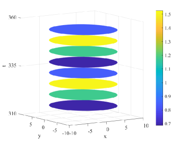
(a) (b)

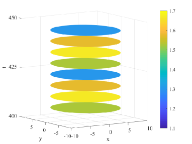
Figure 1: Spatially homogeneous periodic solutions with parameters: $a=1,~{}b=1.5,~{}g=2,~{}d_{1}=2,~{}d_{2}=5,~{}R=10,\tau=2.~{}(a):u,~{}(b):v.$

IV.2 Numerical example 2: A delayed predator-prey model with group defense and nonlocal competition

In (Liu et al., 2020), the authors investigated a predator-prey model with group defence and nonlocal competition. Here, we use the method established above to investigate the dynamics of such a model on a disk.

$$\left\{\begin{array}[]{l}\frac{\partial u(t,r,\theta)}{\partial t}=d_{1}\Delta_{r\theta}u(t,r,\theta)+bu(t,r,\theta)\left(1-\frac{\hat{u}(t,r,\theta)}{K}\right)-au^{\alpha}(t,r,\theta)v(t,r,\theta),~{}(r,\theta)\in\mathbb{D},~{}t>0,\\ \frac{\partial v(t,r,\theta)}{\partial t}=d_{2}\Delta_{r\theta}v(t,r,\theta)-dv(t,r,\theta)+aeu^{\alpha}(t-\tau,r,\theta)v(t,r,\theta),~{}(r,\theta)\in\mathbb{D},~{}t>0,\\ \partial_{r}u(\cdot,R,\theta)=\partial_{r}v(\cdot,R,\theta)=0,~{}\theta\in[0,2\pi),\end{array}\right.$$ (43)

where the state $u$, $v$ and parameters are defined in (Liu et al., 2020). In particular, $\hat{u}(r,\theta,t)$ depicts the nonlocal competition with the form of

$$\hat{u}(r,\theta,t)=\frac{1}{\pi R^{2}}\int_{0}^{R}\int_{0}^{2\pi}\bar{r}u\left(\bar{r},\bar{\theta},t\right)\mathrm{d}\bar{\theta}\mathrm{d}\bar{r}.$$

According to subsection II.2, characteristic equations of the linearization equation at the positive equilibrium point $E^{*}$ for system (43) are

$$\left\{\begin{array}[]{l}\gamma^{2}+P_{0m}\gamma+Q_{0m}-a_{12}b_{21}\mathrm{e}^{-\gamma\tau}=0,~{}m=0,1,2,\cdots,\\ \left(\gamma^{2}+\bar{P}_{nm}\gamma+\bar{Q}_{nm}-a_{12}b_{21}\mathrm{e}^{-\gamma\tau}\right)^{2}=0,~{}n=1,2,\cdots,~{}m=1,2,\cdots,\end{array}\right.$$ (44)

with

$$P_{0m}=(d_{1}+d_{2})\lambda_{0m}^{2}-a_{11}-c_{11},~{}{Q}_{0m}=(d_{1}\lambda_{0m}^{2}-a_{11}-c_{11})d_{2}\lambda_{0m}^{2}~{}m=0,1,2,\cdots;$$

$$\bar{P}_{nm}=(d_{1}+d_{2})\lambda_{nm}^{2}-a_{11},~{}\bar{Q}_{nm}=(d_{1}\lambda_{nm}^{2}-a_{11})d_{2}\lambda_{nm}^{2},~{}n=1,2,\cdots,~{}m=1,2,\cdots,$$

where the expressions of $a_{11},~{}a_{12},~{}b_{21},~{}c_{11}$ are shown in (Liu et al., 2020).

Fixing $b=0.25,~{}K=20,~{}a=0.3,~{}d=0.7,~{}e=0.5,~{}d_{1}=0.3,~{}d_{2}=0.75,~{}R=6$, applying the same mathematical analysis method mentioned in (Ruan and Wei, 2003; Liu et al., 2020), at the unique positive constant steady solution, the first two bifurcation curves on the $\alpha-\tau$ plane are shown in Figure 2. We select $\alpha=0.6$ on the plane of $\alpha-\tau$. When $\hat{\lambda}=\lambda_{11}$, Hopf bifurcation occurs at $\hat{\tau}~{}=\tau_{\lambda_{11}}^{0}\approx 1.7825$. We know that when $\tau~{}\textless~{}1.7825$, $E^{*}$ is locally asymptotically stable, and when $\tau~{}\textgreater~{}1.7825$, $E^{*}$ is unstable. The bifurcation generated at this time is an equivariant hopf bifurcation. It can be obtained through numerical calculation that $\mu=1.2175,~{}B_{11}\approx 0.0021-0.0911\mathrm{i},~{}B_{2001}\approx-0.1075+0.0745\mathrm{i},~{}B_{1110}\approx-0.1813+0.1620\mathrm{i}$. Thus, $a_{1}\mu\approx 0.0026,~{}a_{2}\approx-0.1075,~{}a_{2}+a_{3}\approx-0.2888,~{}a_{2}-a_{3}\approx 0.0738$, which corresponds to Case 2 when $a_{1}\mu>0$ in Table 2. By Theorem III.3, we know that system possesses an unstable standing wave (see Figure 3-5) and two stable rotating waves (see Figure 6-7).

Remark IV.1.

We can see from Figure 2 that as $\alpha$ changes, a double Hopf point HH appears. Below the lower line is the stable region of the system where $\tau~{}\textless~{}min\left\{\tau_{\lambda_{00}^{0}},\tau_{\lambda_{11}^{0}}\right\}$. And above the lower line where $\tau~{}\textgreater~{}\left\{\tau_{\lambda_{00}^{0}},\tau_{\lambda_{11}^{0}}\right\}$ the system may produce spatially homogeneous or inhomogeneous period solutions. Investigating the detailed bifurcation sets might require studying an at least six dimensional center manifold.

Remark IV.2.

We can find that only when the initial value restricted to the center subspace satisfies $\rho_{1}=\rho_{2}$, the spatially inhomogeneous periodic solution is in the form of standing waves. For example, we select the initial value as $u(t,r,\theta)=u^{*}+\varsigma_{1}(t,r)\cdot\cos(\theta+\hat{\theta}),~{}t\in[-\tau,0);~{}v(t,r,\theta)=v^{*}+\varsigma_{2}(t,r)\cdot\cos(\theta+\hat{\theta}),~{}t\in[-\tau,0)$, which has the following approximate form restricted to the center manifold

$$U_{0}(\vartheta)(r,\theta)\approx 4(\mathrm{Re}\{\varsigma_{1}(\vartheta,r)\},\mathrm{Re}\{p_{0}\cdot\varsigma_{2}(\vartheta,r)\})^{\mathrm{T}}\cos(\theta+\hat{\theta}),$$

with $z_{1}=z_{2}=z_{3}=z_{4}=1$. Thus, the spatially inhomogeneous periodic solutions in Figure 3-5 are in the form of standing waves. No matter what value of $\hat{\theta}$ is taken, the simulation is a standing wave solution, which reflects the effect of $O(2)$ equivariance. However, when the initial values of $u$ and $v$ are chosen with other forms, solutions of the system are attracted by one of two coexisting stable rotating waves (see Figure 6-7), which may be clockwise (Figure 7) or counterclockwise (Figure 6).

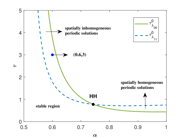
Figure 2: Partial bifurcation curves on the $\alpha-\tau$ plane.

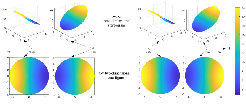
(a) (b)

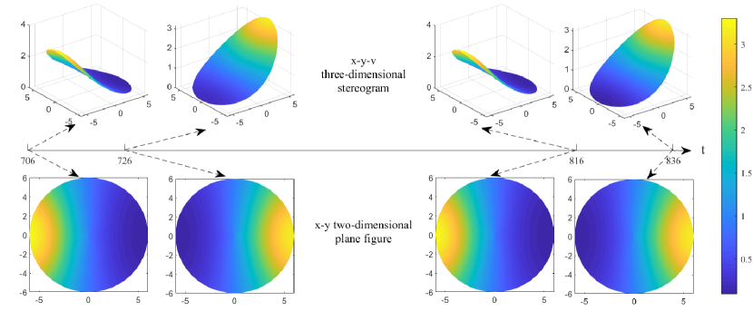
Figure 3: The system produces standing waves with parameters: $b=0.25,~{}K=20,~{}a=0.3,~{}d=0.7,~{}e=0.5,\alpha=0.6,~{}d_{1}=0.3,~{}d_{2}=0.75,~{}R=6,~{}\tau=3$. Initial values are $u(t,r,\theta)=13.0320+0.01\cdot\cos t\cdot\cos r\cdot\cos\theta,~{}v(t,r,\theta)=0.8108+0.01\cdot\cos t\cdot\cos r\cdot\cos\theta,~{}t\in[-\tau,0)$. $(a):u,~{}(b):v$.

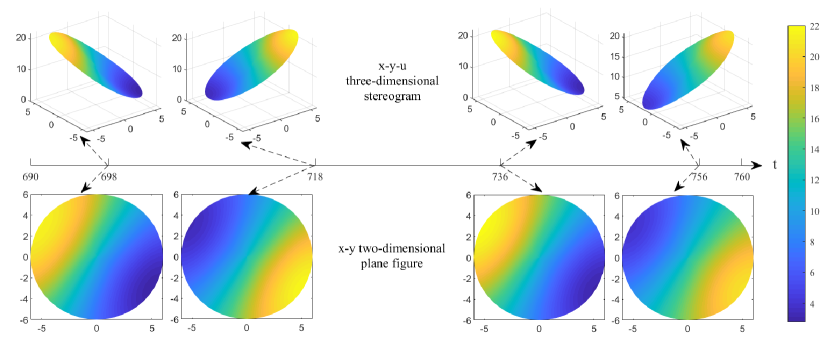
(a) (b)

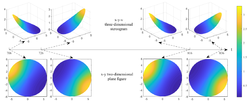
Figure 4: The system produces standing waves with parameters: $b=0.25,~{}K=20,~{}a=0.3,~{}d=0.7,~{}e=0.5,\alpha=0.6,~{}d_{1}=0.3,~{}d_{2}=0.75,~{}R=6,~{}\tau=3$. Initial values are $u(t,r,\theta)=13.0320+0.01\cdot\cos t\cdot\cos r\cdot\cos(\theta+\frac{\pi}{6}),~{}v(t,r,\theta)=0.8108+0.01\cdot\cos t\cdot\cos r\cdot\cos(\theta+\frac{\pi}{6}),~{}t\in[-\tau,0)$. $(a):u,~{}(b):v$.

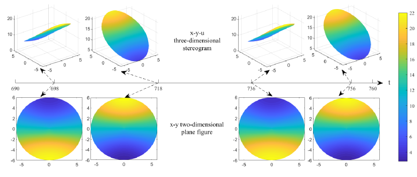
(a) (b)

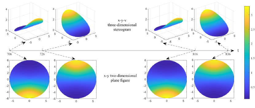
Figure 5: The system produces standing waves with parameters: $b=0.25,~{}K=20,~{}a=0.3,~{}d=0.7,~{}e=0.5,\alpha=0.6,~{}d_{1}=0.3,~{}d_{2}=0.75,~{}R=6,~{}\tau=3$. Initial values are $u(t,r,\theta)=13.0320+0.01\cdot\cos t\cdot\cos r\cdot\cos(\theta-\frac{\pi}{2}),~{}v(t,r,\theta)=0.8108+0.01\cdot\cos t\cdot\cos r\cdot\cos(\theta-\frac{\pi}{2}),~{}t\in[-\tau,0)$. $(a):u,~{}(b):v$.

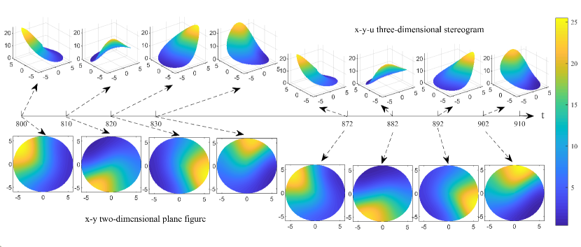
(a) (b)

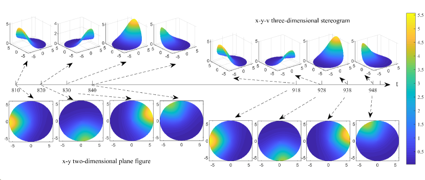
Figure 6: The system produces rotating waves with parameters: $b=0.25,~{}K=20,~{}a=0.3,~{}d=0.7,~{}e=0.5,\alpha=0.6,~{}d_{1}=0.3,~{}d_{2}=0.75,~{}R=6,~{}\tau=3$. Initial values are $u(t,r,\theta)=13.0320+0.01\cdot\cos t\cdot\cos r\cdot\sin\theta,~{}v(t,r,\theta)=0.8108+0.01\cdot\cos t\cdot\cos r\cdot\cos\theta,~{}t\in[-\tau,0)$. $(a):u,~{}(b):v$.

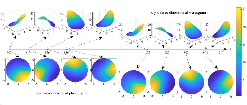
(a) (b)

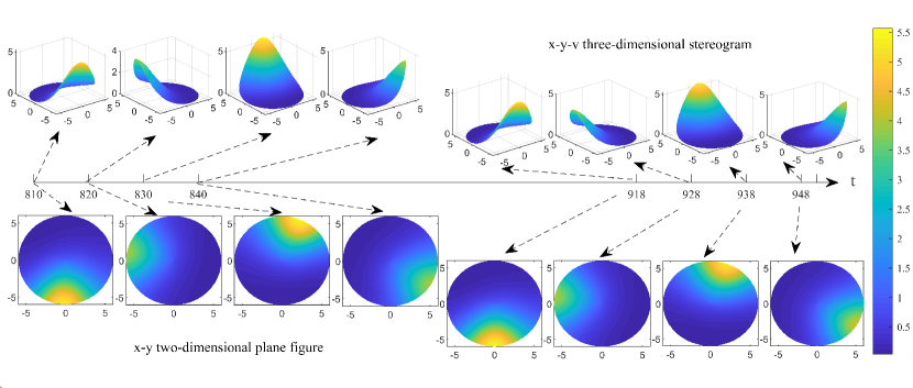
Figure 7: The system produces counterpropagating waves with parameters: $b=0.25,~{}K=20,~{}a=0.3,~{}d=0.7,~{}e=0.5,\alpha=0.6,~{}d_{1}=0.3,~{}d_{2}=0.75,~{}R=6,~{}\tau=3$. Initial values are $u(t,r,\theta)=13.0320+0.01\cdot\cos t\cdot\cos r\cdot\cos\theta,~{}v(t,r,\theta)=0.8108+0.01\cdot\cos t\cdot\cos r\cdot\sin\theta,~{}t\in[-\tau,0)$. $(a):u,~{}(b):v$.

Appendix A The specific calculation of $g_{3}^{1}(z,0,\mu)$

A.1 The calculation of $\mathrm{Proj}_{\mathrm{Ker}(M_{3}^{1})}f_{3}^{1}(z,0,0).$

Writing $\tilde{F}_{3}(\Phi_{r\theta}z,\mu)$ as follows

$$\tilde{F}_{3}(\Phi_{r\theta}z,0)=\sum_{p_{1}+p_{2}+p_{3}+p_{4}=3}A_{p_{1}p_{2}p_{3}p_{4}}\left(\hat{\phi}_{nm}^{c}\right)^{p_{1}+p_{2}}\left({\hat{\phi}_{nm}^{s}}\right)^{p_{3}+p_{4}}z_{1}^{p_{1}}z_{2}^{p_{2}}z_{3}^{p_{3}}z_{4}^{p_{4}},$$

then we have

$$f_{3}^{1}(z,0,0) =\left(\begin{array}[]{cc}\left\langle\tilde{F}_{3}(\Phi_{r\theta}z,0),\Psi_{r\theta}^{1}(0)\right\rangle\\ \left\langle\tilde{F}_{3}(\Phi_{r\theta}z,0),\Psi_{r\theta}^{2}(0)\right\rangle\end{array}\right)$$

$$=\overline{\Psi(0)}\left(\begin{array}[]{cc}\sum_{p_{1}+p_{2}+p_{3}+p_{4}=3}A_{p_{1}p_{2}p_{3}p_{4}}\int_{0}^{R}\int_{0}^{2\pi}r\left(\hat{\phi}_{nm}^{c}\right)^{p_{1}+p_{2}}\left({\hat{\phi}_{nm}^{s}}\right)^{p_{3}+p_{4}+1}\mathrm{d}\theta\mathrm{d}rz_{1}^{p_{1}}z_{2}^{p_{2}}z_{3}^{p_{3}}z_{4}^{p_{4}}\\ \sum_{p_{1}+p_{2}+p_{3}+p_{4}=3}A_{p_{1}p_{2}p_{3}p_{4}}\int_{0}^{R}\int_{0}^{2\pi}r\left(\hat{\phi}_{nm}^{c}\right)^{p_{1}+p_{2}+1}\left({\hat{\phi}_{nm}^{s}}\right)^{p_{3}+p_{4}}\mathrm{d}\theta\mathrm{d}rz_{1}^{p_{1}}z_{2}^{p_{2}}z_{3}^{p_{3}}z_{4}^{p_{4}}\end{array}\right).$$

Noticing the fact

$$\int_{0}^{R}\int_{0}^{2\pi}r\left(\hat{\phi}_{nm}^{c}\right)^{4}\mathrm{d}\theta\mathrm{d}r=\int_{0}^{R}\int_{0}^{2\pi}r\left(\hat{\phi}_{nm}^{s}\right)^{4}\mathrm{d}\theta\mathrm{d}r=0,$$

$$\int_{0}^{R}\int_{0}^{2\pi}r\left(\hat{\phi}_{nm}^{c}\right)^{3}\hat{\phi}_{nm}^{s}\mathrm{d}\theta\mathrm{d}r=\int_{0}^{R}\int_{0}^{2\pi}r\hat{\phi}_{nm}^{c}\left(\hat{\phi}_{nm}^{s}\right)^{3}\mathrm{d}\theta\mathrm{d}r=0,$$

$$\int_{0}^{R}\int_{0}^{2\pi}r\left(\hat{\phi}_{nm}^{c}\right)^{2}\left(\hat{\phi}_{nm}^{s}\right)^{2}\mathrm{d}\theta\mathrm{d}r\triangleq\mathrm{M}_{22},$$

and the relationship of $\Phi_{r\theta}$ and $\Psi_{r\theta}$, we get (31).

A.2 The calculation of $\mathrm{Proj}_{\mathrm{Ker}(M_{3}^{1})}\left(D_{z}f_{2}^{1}(z,0,0)U_{2}^{1}(z,0)\right).$

We have

$$f_{2}^{1}(z,0,0) =\left(\begin{array}[]{cc}\left\langle\tilde{F}_{2}(\Phi_{r\theta}z,0),\Psi_{r\theta}^{1}(0)\right\rangle\\ \left\langle\tilde{F}_{2}(\Phi_{r\theta}z,0),\Psi_{r\theta}^{2}(0)\right\rangle\end{array}\right)$$ (45)

$$=\overline{\Psi(0)}\left(\begin{array}[]{cc}\sum_{p_{1}+p_{2}+p_{3}+p_{4}=2}A_{p_{1}p_{2}p_{3}p_{4}}\int_{0}^{R}\int_{0}^{2\pi}r\left(\hat{\phi}_{nm}^{c}\right)^{p_{1}+p_{2}}\left({\hat{\phi}_{nm}^{s}}\right)^{p_{3}+p_{4}+1}\mathrm{d}\theta\mathrm{d}rz_{1}^{p_{1}}z_{2}^{p_{2}}z_{3}^{p_{3}}z_{4}^{p_{4}}\\ \sum_{p_{1}+p_{2}+p_{3}+p_{4}=2}A_{p_{1}p_{2}p_{3}p_{4}}\int_{0}^{R}\int_{0}^{2\pi}r\left(\hat{\phi}_{nm}^{c}\right)^{p_{1}+p_{2}+1}\left({\hat{\phi}_{nm}^{s}}\right)^{p_{3}+p_{4}}\mathrm{d}\theta\mathrm{d}rz_{1}^{p_{1}}z_{2}^{p_{2}}z_{3}^{p_{3}}z_{4}^{p_{4}}\end{array}\right).$$

Noticing the fact that

$$\int_{0}^{R}\int_{0}^{2\pi}r\left(\hat{\phi}_{nm}^{c}\right)^{3}\mathrm{d}\theta\mathrm{d}r=\int_{0}^{R}\int_{0}^{2\pi}r\left(\hat{\phi}_{nm}^{s}\right)^{3}\mathrm{d}\theta\mathrm{d}r=0,$$

$$\int_{0}^{R}\int_{0}^{2\pi}r\left(\hat{\phi}_{nm}^{c}\right)^{2}\hat{\phi}_{nm}^{s}\mathrm{d}\theta\mathrm{d}r=\int_{0}^{R}\int_{0}^{2\pi}r\hat{\phi}_{nm}^{c}\left(\hat{\phi}_{nm}^{s}\right)^{2}\mathrm{d}\theta\mathrm{d}r=0,$$

then we get $\mathrm{Proj}_{\mathrm{Ker}(M_{3}^{1})}\left(D_{z}f_{2}^{1}(z,0,0)U_{2}^{1}(z,0)\right)=0$.

A.3 The calculation of $\mathrm{Proj}_{\mathrm{Ker}(M_{3}^{1})}\left(D_{y}f_{2}^{1}(z,0,0)U_{2}^{2}(z,0)\right).$

Firstly, we calculate the $\rm{Fr\acute{e}chet}$ derivative $D_{y}f_{2}^{1}(z,0,0):Q_{s}\rightarrow\mathscr{X}_{\mathbb{C}}$. By (26) and (27), $\tilde{F}_{2}(z,y,0)$ can be written as

$$\tilde{F}_{2}(z,y,0) =S_{2}(\Phi_{r\theta}z,y)+o(z^{2},y^{2})$$ (46)

$$=S_{yz_{1}}(y)z_{1}\hat{\phi}_{nm}^{c}+S_{yz_{2}}(y)z_{2}\hat{\phi}_{nm}^{c}+S_{yz_{3}}(y)z_{3}\hat{\phi}_{nm}^{s}+S_{yz_{4}}(y)z_{4}\hat{\phi}_{nm}^{s}+o(z^{2},y^{2}),$$

where $S_{yz_{k}}(k=1,2,3,4):Q_{s}\rightarrow\mathscr{X}_{\mathbb{C}}$ are linear operators, and

$$S_{yz_{k}}(\varphi)=S_{y(0)z_{k}}(\varphi(0))+S_{y(-1)z_{k}}(\varphi(-1)).$$

Let

$$U_{2}^{2}(z,0)\triangleq h(z)=\sum_{j\geq 0}h_{j}(z)\hat{\phi}_{jk}(r,\theta),$$

with

$$h_{jk}(z)=\left(\begin{array}[]{cc}h_{jk}^{(1)}(z)\\ h_{jk}^{(2)}(z)\end{array}\right)=\sum_{p_{1}+p_{2}+p_{3}+p_{4}=2}\left(\begin{array}[]{cc}h_{jkp_{1}p_{2}p_{3}p_{4}}^{(1)}(z)\\ h_{jkp_{1}p_{2}p_{3}p_{4}}^{(2)}(z)\end{array}\right)z_{1}^{p_{1}}z_{2}^{p_{2}}z_{3}^{p_{3}}z_{4}^{p_{4}}.$$

Therefore,

$$D_{y}\tilde{F}_{2}(z,0,0)\left(U_{2}^{2}(z,0)\right) =\left(\begin{array}[]{cc}\langle D_{y}\tilde{F}_{2}(z,0,0)\left(U_{2}^{2}(z,0)\right),\Psi_{r\theta}^{1}(0)\rangle\\ \langle D_{y}\tilde{F}_{2}(z,0,0)\left(U_{2}^{2}(z,0)\right),\Psi_{r\theta}^{2}(0)\rangle\end{array}\right)$$

$$=\overline{\Psi(0)}\left(\begin{array}[]{cc}\sum_{j\geq 0}\left[\mathrm{M}_{jkcs}S_{yz_{1}}(h_{jk})z_{1}+\mathrm{M}_{jkcs}S_{yz_{2}}(h_{jk})z_{2}\right.\\ \left.+\mathrm{M}_{jkss}S_{yz_{3}}(h_{jk})z_{3}+\mathrm{M}_{jkss}S_{yz_{4}}(h_{jk})z_{4}\right]\\ \sum_{j\geq 0}[\mathrm{M}_{jkcc}S_{yz_{1}}(h_{jk})z_{1}+\mathrm{M}_{jkcc}S_{yz_{2}}(h_{jk})z_{2}\\ +\mathrm{M}_{jksc}S_{yz_{3}}(h_{jk})z_{3}+\mathrm{M}_{jksc}S_{yz_{4}}(h_{jk})z_{4}]\end{array}\right),$$

where

$$\mathrm{M}_{jksc}=\mathrm{M}_{jkcs}=\int_{0}^{R}\int_{0}^{2\pi}r\hat{\phi}_{jk}\hat{\phi}_{nm}^{c}\hat{\phi}_{nm}^{s}\mathrm{d}\theta\mathrm{d}r=\left\{\begin{array}[]{cccc}\mathrm{M}_{0kcs}^{c}&\hat{\phi}_{0}~{}or~{}\hat{\phi}_{0k}^{c},\\ 0,&otherwise,\end{array}\right.$$

$$\mathrm{M}_{jkss}=\int_{0}^{R}\int_{0}^{2\pi}r\hat{\phi}_{jk}\hat{\phi}_{nm}^{s}\hat{\phi}_{nm}^{s}\mathrm{d}\theta\mathrm{d}r=\left\{\begin{array}[]{cccc}\mathrm{M}_{2nkss}^{c},&\hat{\phi}_{jk}=\hat{\phi}_{2nk}^{c},\\ 0,&otherwise,\end{array}\right.$$

$$\mathrm{M}_{jkcc}=\int_{0}^{R}\int_{0}^{2\pi}r\hat{\phi}_{jk}\hat{\phi}_{nm}^{c}\hat{\phi}_{nm}^{c}\mathrm{d}\theta\mathrm{d}r=\left\{\begin{array}[]{cccc}\mathrm{M}_{2nkcc}^{s},&\hat{\phi}_{jk}=\hat{\phi}_{2nk}^{s},\\ 0,&otherwise.\end{array}\right.$$

Moreover, we have

$$D_{y}\tilde{F}_{2}(z,0,0)\left(U_{2}^{2}(z,0)\right) =\bar{\Psi}(0)\left(\begin{array}[]{cccc}N_{1}\\ N_{2}\end{array}\right),$$

with

$$N_{1}= \mathrm{M}_{0kcs}^{c}\left(S_{yz_{1}}(h_{0k}^{ccs})z_{1}+S_{yz_{2}}(h_{0k}^{ccs})z_{2}\right)+\mathrm{M}_{2nkss}^{c}\left(S_{yz_{3}}(h_{2nk}^{css})z_{3}+S_{yz_{4}}(h_{2nk}^{css})z_{4}\right),$$

$$N_{2}= \mathrm{M}_{2nkcc}^{s}\left(S_{yz_{1}}(h_{2nk}^{ccs})z_{1}+S_{yz_{2}}(h_{2nk}^{ccs})z_{2}\right)+\mathrm{M}_{0kcs}^{c}\left(S_{yz_{3}}(h_{0k}^{ccs})z_{3}+S_{yz_{4}}(h_{0k}^{ccs})z_{4}\right).$$

Thus,

$$\frac{1}{3!}\mathrm{Proj}_{\mathrm{Ker(M_{3}^{1})}}\left(D_{y}f_{2}^{1}(z,0,0)U_{2}^{2}(z,0)\right)$$ (47)

$$= \left(\begin{array}[]{cccc}E_{2100}^{1}z_{1}^{2}z_{2}+E_{2001}^{1}z_{1}^{2}z_{4}+E_{0120}^{1}z_{3}^{2}z_{2}+E_{0021}^{1}z_{3}^{2}z_{4}+E_{1110}^{1}z_{1}z_{2}z_{3}+E_{1011}^{1}z_{1}z_{3}z_{4}\\ \overline{E_{2100}^{1}}z_{1}z_{2}^{2}+\overline{E_{2001}^{1}}z_{2}^{2}z_{3}+\overline{E_{0120}^{1}}z_{4}^{2}z_{1}+\overline{E_{0021}^{1}}z_{3}z_{4}^{2}+\overline{E_{1110}^{1}}z_{1}z_{2}z_{4}+\overline{E_{1011}^{1}}z_{2}z_{3}z_{4}\\ E_{2100}^{2}z_{1}^{2}z_{2}+E_{2001}^{2}z_{1}^{2}z_{4}+E_{0120}^{2}z_{3}^{2}z_{2}+E_{0021}^{2}z_{3}^{2}z_{4}+E_{1110}^{2}z_{1}z_{2}z_{3}+E_{1011}^{2}z_{1}z_{3}z_{4}\\ \overline{E_{2100}^{2}}z_{1}z_{2}^{2}+\overline{E_{2001}^{2}}z_{2}^{2}z_{3}+\overline{E_{0120}^{2}}z_{4}^{2}z_{1}+\overline{E_{0021}^{2}}z_{3}z_{4}^{2}+\overline{E_{1110}^{2}}z_{1}z_{2}z_{4}+\overline{E_{1011}^{2}}z_{2}z_{3}z_{4}\end{array}\right),$$

where

$$E_{2100}^{1}=\frac{1}{6}\overline{\Psi_{1}(0)} \left[\mathrm{M}_{0kcs}^{c}\left(S_{yz_{1}}(h_{0k1100}^{ccs})+S_{yz_{2}}(h_{0k2000}^{ccs})\right)\right],$$

$$E_{2001}^{1}=\frac{1}{6}\overline{\Psi_{1}(0)} \left[\mathrm{M}_{0kcs}^{c}S_{yz_{1}}(h_{0k1001}^{ccs})+\mathrm{M}_{2nkss}^{c}S_{yz_{4}}(h_{2nk2000}^{css})\right],$$

$$E_{0120}^{1}=\frac{1}{6}\overline{\Psi_{1}(0)} \left[\mathrm{M}_{0kcs}^{c}S_{yz_{2}}(h_{0k0020}^{ccs}))+\mathrm{M}_{2nkss}^{c}S_{yz_{3}}(h_{2nk0110}^{css})\right],$$

$$E_{0021}^{1}=\frac{1}{6}\overline{\Psi_{1}(0)} \left[\mathrm{M}_{2nkss}^{c}\left(S_{yz_{3}}(h_{2nk0011}^{css})+S_{yz_{4}}(h_{2nk0020}^{css})\right)\right],$$

$$E_{1110}^{1}=\frac{1}{6}\overline{\Psi_{1}(0)} \left[\mathrm{M}_{0kcs}^{c}\left(S_{yz_{1}}(h_{0k0110}^{ccs})+S_{yz_{2}}(h_{0k1010}^{ccs})\right)+\mathrm{M}_{2nkss}^{c}S_{yz_{3}}(h_{2nk1100}^{css})\right],$$

$$E_{1011}^{1}=\frac{1}{6}\overline{\Psi_{1}(0)} \left[\mathrm{M}_{0kcs}^{c}S_{yz_{1}}(h_{0k0011}^{ccs})+\mathrm{M}_{2nkss}^{c}\left(S_{yz_{3}}(h_{2nk1001}^{css})+S_{yz_{4}}(h_{2nk1010}^{css})\right)\right],$$

$$E_{2100}^{2}=\frac{1}{6}\overline{\Psi_{3}(0)} \left[\mathrm{M}_{2nkcc}^{s}\left(S_{yz_{1}}(h_{2nk1100}^{ccs})+S_{yz_{2}}(h_{2nk2000}^{ccs})\right)\right],$$

$$E_{2001}^{2}=\frac{1}{6}\overline{\Psi_{3}(0)} \left[\mathrm{M}_{2nkcc}^{s}S_{yz_{1}}(h_{2nk1001}^{ccs})+\mathrm{M}_{0kcs}^{c}S_{yz_{2}}(h_{0k2000}^{ccs})\right],$$

$$E_{0120}^{2}=\frac{1}{6}\overline{\Psi_{3}(0)} \left[\mathrm{M}_{2nkcc}^{s}S_{yz_{2}}(h_{2nk0020}^{ccs})+\mathrm{M}_{0kcs}^{c}S_{yz_{3}}(h_{0k0110}^{ccs})\right],$$

$$E_{0021}^{2}=\frac{1}{6}\overline{\Psi_{3}(0)} \left[\mathrm{M}_{0kcs}^{c}\left(S_{yz_{3}}(h_{0k0011}^{ccs})+S_{yz_{4}}(h_{0k0020}^{ccs})\right)\right],$$

$$E_{1110}^{2}=\frac{1}{6}\overline{\Psi_{3}(0)} \left[\mathrm{M}_{2nkcc}^{s}\left(S_{yz_{1}}(h_{2nk0110}^{ccs})+S_{yz_{2}}(h_{2nk1010}^{ccs})\right)+\mathrm{M}_{0kcs}^{c}S_{yz_{3}}(h_{0k1100}^{ccs})\right]$$

$$E_{1011}^{2}=\frac{1}{6}\overline{\Psi_{3}(0)} \left[\mathrm{M}_{2nkcc}^{s}S_{yz_{1}}(h_{2nk0011}^{ccs})+\mathrm{M}_{0kcs}^{c}\left(S_{yz_{3}}(h_{0k1001}^{ccs})+S_{yz_{4}}(h_{0k1010}^{ccs})\right)\right].$$

Now, we need to calculate

$$h_{0k2000}^{ccs},~{}h_{0k1100}^{ccs},~{}h_{0k1010}^{ccs},~{}h_{0k1001}^{ccs},~{}h_{0k0110}^{ccs},~{}h_{0k0020}^{ccs},~{}h_{0k0011}^{ccs},$$

$$h_{2nk2000}^{ccs},~{}h_{2nk1100}^{ccs},~{}h_{2nk1010}^{ccs},~{}h_{2nk1001}^{ccs},~{}h_{2nk0110}^{ccs},~{}h_{2nk0020}^{ccs},~{}h_{2nk0011}^{ccs},$$

$$h_{2nk2000}^{css},~{}h_{2nk1100}^{css},~{}h_{2nk1010}^{css},~{}h_{2nk1001}^{css},~{}h_{2nk0110}^{css},~{}h_{2nk0020}^{css},~{}h_{2nk0011}^{css}.$$

From (19) and(24), we get

$$M_{2}^{2}U_{2}^{2}(z,0)(\vartheta) =M_{2}^{2}h(z)(\vartheta)$$

$$=\left\{\begin{array}[]{cc}D_{z}h(z)Bz-\tilde{D}_{0}\Delta h(0)-\tilde{L}_{0}(h(z)),&\vartheta=0,\\ D_{z}h(z)Bz-D_{\vartheta}h(z),&\vartheta\neq 0,\\ \end{array}\right.$$

$$=\left\{\begin{array}[]{cc}\sum_{j\geq 0}\left[D_{z}h_{j}(z)\hat{\phi}_{jk}(r,\theta)Bz-\tilde{D}_{0}\Delta h_{j}(z)\hat{\phi}_{jk}(r,\theta)-\tilde{L}_{0}(h_{j}(z)\hat{\phi}_{jk}(r,\theta))\right],&\vartheta=0,\\ \sum_{j\geq 0}\left[D_{z}h_{j}(z)\hat{\phi}_{jk}(r,\theta)Bz-D_{\vartheta}h_{j}(z)\hat{\phi}_{jk}(r,\theta)\right],&\vartheta\neq 0,\\ \end{array}\right.$$

and

$$f_{2}^{2}(z,0,0)=\left\{\begin{array}[]{cc}\begin{aligned} \tilde{F}_{2}&(z,0,0)-\Phi_{1}(0)f_{2}^{1(1)}(z,0,0)\hat{\phi}_{nm}^{s}-\Phi_{2}(0)f_{2}^{1(2)}(z,0,0)\hat{\phi}_{nm}^{s}\\ &-\Phi_{3}(0)f_{2}^{1(1)}(z,0,0)\hat{\phi}_{nm}^{c}-\Phi_{4}(0)f_{2}^{1(1)}(z,0,0)\hat{\phi}_{nm}^{c},&\vartheta=0,\\ -\Phi_{1}&(\vartheta)f_{2}^{1(1)}(z,0,0)\hat{\phi}_{nm}^{s}-\Phi_{2}(\vartheta)f_{2}^{1(2)}(z,0,0)\hat{\phi}_{nm}^{s}\\ &-\Phi_{3}(\vartheta)f_{2}^{1(1)}(z,0,0)\hat{\phi}_{nm}^{c}-\Phi_{4}(\vartheta)f_{2}^{1(1)}(z,0,0)\hat{\phi}_{nm}^{c},&\vartheta\neq 0.\end{aligned}\end{array}\right.$$

Besides, we have

$$\langle M_{2}^{2}\left(U_{2}^{2}(z,0)\right),\beta_{jk}\rangle=\langle f_{2}^{2}(z,0,0),\beta_{jk}\rangle,$$ (48)

with $\beta_{jk}=\frac{\phi_{jk}}{\|\phi_{jk}\|}$.

Thus, the expressions of $h_{jp_{1}p_{2}p_{3}p_{4}}$ can be obtained. Due to the large number of expressions, we show the specific results in the Appendix F.

Noting the fact that

$$\mathrm{M}_{2nkcc}^{s}=\mathrm{M}_{2nkss}^{c},$$

therefore, we have

$$E_{2100}^{1}=E_{0021}^{2},~{}E_{2001}^{1}=E_{0120}^{2},~{}E_{0120}^{1}=E_{2001}^{2},$$

$$E_{0021}^{1}=E_{2100}^{2},~{}E_{1110}^{1}=E_{1011}^{2},~{}E_{1011}^{1}=E_{1110}^{2},$$

For simplification of notations, we rewrite (47) as (34).

Appendix B Proof of Lemma III.2

By a smooth transformation

$$z_{1}=\zeta_{1}+b_{1}\zeta_{1}^{2}\zeta_{2}+b_{2}\zeta_{3}^{2}\zeta_{2}+b_{3}\zeta_{3}^{2}\zeta_{4}+b_{4}\zeta_{1}\zeta_{3}\zeta_{4},$$ (49)

$$z_{2}=\bar{z}_{1},$$

$$z_{3}=\zeta_{1}+b_{1}\zeta_{3}^{2}\zeta_{4}+b_{2}\zeta_{1}^{2}\zeta_{4}+b_{3}\zeta_{1}^{2}\zeta_{2}+b_{4}\zeta_{1}\zeta_{2}\zeta_{3},$$

$$z_{4}=\bar{z}_{3},$$

we have

$$\zeta_{1}=z_{1}-b_{1}z_{1}^{2}z_{2}-b_{2}z_{3}^{2}z_{2}-b_{3}z_{3}^{2}z_{4}-b_{4}z_{1}z_{3}z_{4}+o(4),$$ (50)

$$\zeta_{2}=\bar{\zeta}_{1},$$

$$\zeta_{3}=z_{1}-b_{1}z_{3}^{2}z_{4}-b_{2}z_{1}^{2}z_{4}-b_{3}z_{1}^{2}z_{2}-b_{4}z_{1}z_{2}z_{3}+o(4),$$

$$\zeta_{4}=\bar{\zeta}_{3}.$$

Then

$$\dot{\zeta}_{1}= \dot{z}_{1}-2b_{1}z_{1}z_{2}\dot{z}_{1}-b_{1}z_{1}^{2}\dot{z}_{2}-2b_{2}z_{2}z_{3}\dot{z}_{3}-b_{2}z_{3}^{2}\dot{z}_{2}-2b_{3}z_{3}z_{4}\dot{z}_{3}-b_{3}z_{3}^{2}\dot{z}_{4}-b_{4}z_{1}z_{3}\dot{z}_{4}-b_{4}z_{1}z_{4}\dot{z}_{3}-b_{4}z_{3}z_{4}\dot{z}_{1}+o(4)$$

$$= (\mathrm{i}\omega_{\hat{\lambda}}+B_{11}\mu)z_{1}+B_{2100}z_{1}^{2}z_{2}^{2}+B_{1011}z_{1}z_{3}z_{4}+B_{2001}z_{1}^{2}z_{4}+B_{0120}z_{3}^{2}z_{2}+B_{0021}z_{3}^{2}z_{4}+B_{1110}z_{1}z_{2}z_{3}$$

$$-3b_{1}(\mathrm{i}\omega_{\hat{\lambda}}+B_{11}\mu)z_{1}^{2}z_{2}-3b_{2}(\mathrm{i}\omega_{\hat{\lambda}}+B_{11}\mu)z_{3}^{2}z_{2}-3b_{3}(\mathrm{i}\omega_{\hat{\lambda}}+B_{11}\mu)z_{3}^{2}z_{4}-3b_{4}(\mathrm{i}\omega_{\hat{\lambda}}+B_{11}\mu)z_{1}z_{3}z_{4}+o(4).$$

Let

$$b_{1}=\frac{B_{2100}}{3(\mathrm{i}\omega_{\hat{\lambda}}+B_{11}\mu)},~{}b_{2}=\frac{B_{0120}}{3(\mathrm{i}\omega_{\hat{\lambda}}+B_{11}\mu)},$$

$$b_{3}=\frac{B_{0021}}{3(\mathrm{i}\omega_{\hat{\lambda}}+B_{11}\mu)},~{}b_{4}=\frac{B_{1011}}{3(\mathrm{i}\omega_{\hat{\lambda}}+B_{11}\mu)},$$

then

$$\dot{\zeta}_{1}= (\mathrm{i}\omega_{\hat{\lambda}}+B_{11}\mu)z_{1}+B_{2001}z_{1}^{2}z_{4}^{2}+B_{1110}z_{1}z_{2}z_{3}+o(4)$$

$$= (\mathrm{i}\omega_{\hat{\lambda}}+B_{11}\mu)\zeta_{1}+B_{2001}\zeta_{1}^{2}\zeta_{4}^{2}+B_{1110}\zeta_{1}\zeta_{2}\zeta_{3}+o(4).$$

The same is true for $\dot{\zeta}_{2},\dot{\zeta}_{3}$ and $\dot{\zeta}_{4}$ so that (37) is established.

Appendix C Proof of Theorem III.3

We only need to prove the approximate expressions of rotating and standing wave solutions reduced to the center subspace, and the rest of the theorem can be easily obtained from previous analysis.

By (16), (18),(38), we get

$$U_{t}(\vartheta)(r,\theta)\approx \xi\mathrm{e}^{\mathrm{i}\omega_{\hat{\lambda}}\vartheta}J_{n}(\sqrt{\lambda_{nm}}r)\mathrm{e}^{\mathrm{i}n\theta}\rho_{1}\mathrm{e}^{\mathrm{i}\chi_{1}(t)}+\bar{\xi}\mathrm{e}^{-\mathrm{i}\omega_{\hat{\lambda}}\vartheta}J_{n}(\sqrt{\lambda_{nm}}r)\mathrm{e}^{\mathrm{i}n\theta}\rho_{2}\mathrm{e}^{-\mathrm{i}\chi_{2}(t)}$$

$$+\xi\mathrm{e}^{\mathrm{i}\omega_{\hat{\lambda}}\vartheta}J_{n}(\sqrt{\lambda_{nm}}r)\mathrm{e}^{-\mathrm{i}n\theta}\rho_{2}\mathrm{e}^{\mathrm{i}\chi_{2}(t)}+\bar{\xi}\mathrm{e}^{-\mathrm{i}\omega_{\hat{\lambda}}\vartheta}J_{n}(\sqrt{\lambda_{nm}}r)\mathrm{e}^{-\mathrm{i}n\theta}\rho_{1}\mathrm{e}^{-\mathrm{i}\chi_{1}(t)}$$

with $\xi=(p_{11},p_{12},\cdots,p_{1n})^{\mathrm{T}}$. For simplicity, we also rewrite $p_{1i}$ in the form of a complex angle as $p_{1i}=|p_{1i}|\mathrm{e}^{\mathrm{i}\mathrm{Arg}(p_{1i})}$ in the subsequent calculations.

For $(\rho_{1},\rho_{2})=(0,\sqrt{\frac{-a_{1}\mu}{a_{2}}})$,

$$U_{t}(\vartheta)(r,\theta)\approx \xi\mathrm{e}^{\mathrm{i}\omega_{\hat{\lambda}}\vartheta}J_{n}(\sqrt{\lambda_{nm}}r)\mathrm{e}^{\mathrm{i}n\theta}\rho_{1}\mathrm{e}^{\mathrm{i}\chi_{1}(t)}+\bar{\xi}\mathrm{e}^{-\mathrm{i}\omega_{\hat{\lambda}}\vartheta}J_{n}(\sqrt{\lambda_{nm}}r)\mathrm{e}^{-\mathrm{i}n\theta}\rho_{1}\mathrm{e}^{-\mathrm{i}\chi_{1}(t)}$$

$$\approx \sum_{i=1}^{n}{2|p_{1i}|\sqrt{\frac{-a_{1}\mu}{a_{2}}}J_{n}(\sqrt{\lambda_{nm}}r)\cos(\mathrm{Arg}(p_{1i})+\omega_{\hat{\lambda}}\vartheta+\omega_{\hat{\lambda}}t+n\theta){e}_{i}}.$$

where $e_{i}$ is the $i$th unit coordinate vector of $\mathbb{R}^{n}$. This corresponds to the form of a rotating wave solution in the plane of $(z_{2},z_{3})$.

For $(\rho_{1},\rho_{2})=(\sqrt{\frac{-a_{1}\mu}{a_{2}}},0)$,

$$U_{t}(\vartheta)(r,\theta)\approx \bar{\xi}\mathrm{e}^{-\mathrm{i}\omega_{\hat{\lambda}}\vartheta}J_{n}(\sqrt{\lambda_{nm}}r)\mathrm{e}^{\mathrm{i}n\theta}\rho_{2}\mathrm{e}^{-\mathrm{i}\chi_{2}(t)}+\xi\mathrm{e}^{\mathrm{i}\omega_{\hat{\lambda}}\vartheta}J_{n}(\sqrt{\lambda_{nm}}r)\mathrm{e}^{-\mathrm{i}n\theta}\rho_{2}\mathrm{e}^{\mathrm{i}\chi_{2}(t)}$$

$$\approx \sum_{i=1}^{n}{2|p_{1i}|\sqrt{\frac{-a_{1}\mu}{a_{2}}}J_{n}(\sqrt{\lambda_{nm}}r)\cos(\mathrm{Arg}(p_{1i})+\omega_{\hat{\lambda}}\vartheta+\omega_{\hat{\lambda}}t-n\theta){e}_{i}},$$

which corresponds to the form of a rotating wave solution in the opposite direction in the plane of $(z_{1},z_{4})$.

For $(\rho_{1},\rho_{2})=(\sqrt{\frac{-a_{1}\mu}{a_{2}+a_{3}}},\sqrt{\frac{-a_{1}\mu}{a_{2}+a_{3}}})$,

$$U_{t}(\vartheta)(r,\theta)\approx \sum_{i=1}^{n}{2|p_{1i}|\sqrt{\frac{-a_{1}\mu}{a_{2}+a_{3}}}J_{n}(\sqrt{\lambda_{nm}}r)\cos(\mathrm{Arg}(p_{1i})+\omega_{\hat{\lambda}}\vartheta+\omega_{\hat{\lambda}}t+n\theta){e}_{i}}$$

$$+ \sum_{i=1}^{n}{2|p_{1i}|\sqrt{\frac{-a_{1}\mu}{a_{2}+a_{3}}}J_{n}(\sqrt{\lambda_{nm}}r)\cos(\mathrm{Arg}(p_{1i})+\omega_{\hat{\lambda}}\vartheta+\omega_{\hat{\lambda}}t-n\theta){e}_{i}}$$

$$\approx \sum_{i=1}^{n}{4|p_{1i}|\sqrt{\frac{-a_{1}\mu}{a_{2}+a_{3}}}J_{n}(\sqrt{\lambda_{nm}}r)\cos(\mathrm{Arg}(p_{1i})+\omega_{\hat{\lambda}}\vartheta+\omega_{\hat{\lambda}}t)\cos(n\theta){e}_{i}},$$

which means when $n\theta=\frac{\pi}{2}$ or $n\theta=\frac{3\pi}{2}$, the form of the solution does not change over time. In other words, in a two-dimensional plane, the image of the solution has a fixed axis, thus, it corresponds to the form of a standing wave solution.

Appendix D The calculation formula for $A_{p_{1}p_{2}p_{3}p_{4}}$

D.1 The calculation formula for $A_{p_{1}p_{2}p_{3}p_{4}}(p_{1}+p_{2}+p_{3}+p_{4}=2)$

$$A_{2000}=2\hat{\tau}\left(\begin{array}[]{cccc}A_{2000}^{1}\\ A_{2000}^{2}\end{array}\right) ,~{}A_{1100}=2\hat{\tau}\left(\begin{array}[]{cccc}A_{1100}^{1}\\ A_{1100}^{2}\end{array}\right),$$

$$A_{1010}=2\hat{\tau}\left(\begin{array}[]{cccc}A_{1010}^{1}\\ A_{1010}^{2}\end{array}\right) ,~{}A_{1001}=2\hat{\tau}\left(\begin{array}[]{cccc}A_{1001}^{1}\\ A_{1001}^{2}\end{array}\right),$$

$$A_{0020}=2\hat{\tau}\left(\begin{array}[]{cccc}A_{0020}^{1}\\ A_{0020}^{2}\end{array}\right) ,~{}A_{0011}=2\hat{\tau}\left(\begin{array}[]{cccc}A_{0011}^{1}\\ A_{0011}^{2}\end{array}\right),$$

$$A_{0200}=\overline{A_{2000}} ,~{}A_{0101}=\overline{A_{1010}},$$

$$A_{0110}=\overline{A_{1001}} ,~{}A_{0002}=\overline{A_{0020}},$$

with

$$A_{2000}^{1}= F_{20}^{(1)}+F_{11}^{(1)}p_{0}+F_{02}^{(1)}p_{0}^{2},$$

$$A_{1100}^{1}= 2F_{20}^{(1)}+F_{11}^{(1)}(p_{0}+\bar{p}_{0})+2F_{02}^{(1)}p_{0}\bar{p}_{0},$$

$$A_{1010}^{1}= 2F_{20}^{(1)}+2F_{11}^{(1)}p_{0}+2F_{02}^{(1)}p_{0}^{2},$$

$$A_{1001}^{1}= 2F_{20}^{(1)}+F_{11}^{(1)}(p_{0}+\bar{p}_{0})+2F_{02}^{(1)}p_{0}\bar{p}_{0},$$

$$A_{0020}^{1}= F_{20}^{(1)}+F_{11}^{(1)}{p}_{0}+F_{02}^{(1)}p_{0}^{2},$$

$$A_{0011}^{1}= 2F_{20}^{(1)}+F_{11}^{(1)}(p_{0}+\bar{p}_{0})+2F_{02}^{(1)}p_{0}\bar{p}_{0},$$

$$A_{2000}^{2}= F_{2000}^{(2)}+F_{1100}^{(2)}p_{0}+F_{0200}^{(2)}p_{0}^{2}+F_{0020}^{(2)}\mathrm{e}^{-2\mathrm{i}\omega_{\hat{\lambda}}\hat{\tau}}+F_{0011}^{(2)}p_{0}\mathrm{e}^{-2\mathrm{i}\omega_{\hat{\lambda}}\hat{\tau}}+F_{0002}^{(2)}p_{0}^{2}\mathrm{e}^{-2\mathrm{i}\omega_{\hat{\lambda}}\hat{\tau}}$$

$$+F_{1010}^{(2)}\mathrm{e}^{-\mathrm{i}\omega_{\hat{\lambda}}\hat{\tau}}+(F_{1001}^{(2)}+F_{0110}^{(2)})p_{0}\mathrm{e}^{-\mathrm{i}\omega_{\hat{\lambda}}\hat{\tau}}+F_{0101}^{(2)}p_{0}^{2}\mathrm{e}^{-\mathrm{i}\omega_{\hat{\lambda}}\hat{\tau}},$$

$$A_{1100}^{2}= 2F_{2000}^{(2)}+F_{1100}^{(2)}(p_{0}+\bar{p}_{0})+2F_{0200}^{(1)}p_{0}\bar{p}_{0}+2F_{0020}^{(2)}+F_{0011}^{(2)}(p_{0}+\bar{p}_{0})+2F_{0002}^{(2)}p_{0}\bar{p}_{0}+F_{1010}^{(2)}(\mathrm{e}^{-\mathrm{i}\omega_{\hat{\lambda}}\hat{\tau}}+\mathrm{e}^{\mathrm{i}\omega_{\hat{\lambda}}\hat{\tau}})$$

$$+F_{1001}^{(2)}(p_{0}\mathrm{e}^{-\mathrm{i}\omega_{\hat{\lambda}}\hat{\tau}}+\bar{p}_{0}\mathrm{e}^{\mathrm{i}\omega_{\hat{\lambda}}\hat{\tau}})+F_{0110}^{(2)}(p_{0}\mathrm{e}^{\mathrm{i}\omega_{\hat{\lambda}}\hat{\tau}}+\bar{p}_{0}\mathrm{e}^{-\mathrm{i}\omega_{\hat{\lambda}}\hat{\tau}})+F_{0101}^{(2)}(p_{0}\bar{p}_{0}\mathrm{e}^{\mathrm{i}\omega_{\hat{\lambda}}\hat{\tau}}+p_{0}\bar{p}_{0}\mathrm{e}^{-\mathrm{i}\omega_{\hat{\lambda}}\hat{\tau}}),$$

$$A_{1010}^{2}= 2F_{2000}^{(2)}+2F_{1100}^{(2)}p_{0}+2F_{0200}^{(1)}p_{0}^{2}+2F_{0020}^{(2)}\mathrm{e}^{-2\mathrm{i}\omega_{\hat{\lambda}}\hat{\tau}}+2F_{0011}^{(2)}p_{0}\mathrm{e}^{-2\mathrm{i}\omega_{\hat{\lambda}}\hat{\tau}}+2F_{0002}^{(2)}p_{0}^{2}\mathrm{e}^{-2\mathrm{i}\omega_{\hat{\lambda}}\hat{\tau}}$$

$$+2F_{1010}^{(2)}\mathrm{e}^{-\mathrm{i}\omega_{\hat{\lambda}}\hat{\tau}}+2(F_{1001}^{(2)}+F_{0110}^{(2)})p_{0}\mathrm{e}^{-\mathrm{i}\omega_{\hat{\lambda}}\hat{\tau}}+2F_{0101}^{(2)}p_{0}^{2}\mathrm{e}^{-\mathrm{i}\omega_{\hat{\lambda}}\hat{\tau}},$$

$$A_{1001}^{2}= 2F_{2000}^{(2)}+F_{1100}^{(2)}(p_{0}+\bar{p}_{0})+2F_{0200}^{(1)}p_{0}\bar{p}_{0}+2F_{0020}^{(2)}+F_{0011}^{(2)}(p_{0}+\bar{p}_{0})+2F_{0002}^{(2)}p_{0}\bar{p}_{0}+F_{1010}^{(2)}(\mathrm{e}^{-\mathrm{i}\omega_{\hat{\lambda}}\hat{\tau}}+\mathrm{e}^{\mathrm{i}\omega_{\hat{\lambda}}\hat{\tau}})$$

$$+F_{1001}^{(2)}(p_{0}\mathrm{e}^{-\mathrm{i}\omega_{\hat{\lambda}}\hat{\tau}}+\bar{p}_{0}\mathrm{e}^{\mathrm{i}\omega_{\hat{\lambda}}\hat{\tau}})+F_{0110}^{(2)}(p_{0}\mathrm{e}^{\mathrm{i}\omega_{\hat{\lambda}}\hat{\tau}}+\bar{p}_{0}\mathrm{e}^{-\mathrm{i}\omega_{\hat{\lambda}}\hat{\tau}})+F_{0101}^{(2)}(p_{0}\bar{p}_{0}\mathrm{e}^{\mathrm{i}\omega_{\hat{\lambda}}\hat{\tau}}+p_{0}\bar{p}_{0}\mathrm{e}^{-\mathrm{i}\omega_{\hat{\lambda}}\hat{\tau}}),$$

$$A_{0020}^{2}= F_{2000}^{(2)}+F_{1100}^{(2)}p_{0}+F_{0200}^{(2)}p_{0}^{2}+F_{0020}^{(2)}\mathrm{e}^{-2\mathrm{i}\omega_{\hat{\lambda}}\hat{\tau}}+F_{0011}^{(2)}p_{0}\mathrm{e}^{-2\mathrm{i}\omega_{\hat{\lambda}}\hat{\tau}}+F_{0002}^{(2)}p_{0}^{2}\mathrm{e}^{-2\mathrm{i}\omega_{\hat{\lambda}}\hat{\tau}}$$

$$+F_{1010}^{(2)}\mathrm{e}^{-\mathrm{i}\omega_{\hat{\lambda}}\hat{\tau}}+(F_{1001}^{(2)}+F_{1001}^{(2)})p_{0}\mathrm{e}^{-\mathrm{i}\omega_{\hat{\lambda}}\hat{\tau}}+F_{0101}^{(2)}p_{0}^{2}\mathrm{e}^{-\mathrm{i}\omega_{\hat{\lambda}}\hat{\tau}},$$

$$A_{0011}^{2}= 2F_{2000}^{(2)}+F_{1100}^{(2)}(p_{0}+\bar{p}_{0})+2F_{0200}^{(1)}p_{0}\bar{p}_{0}+2F_{0020}^{(2)}+F_{0011}^{(2)}(p_{0}+\bar{p}_{0})+2F_{0002}^{(2)}p_{0}\bar{p}_{0}+F_{1010}^{(2)}(\mathrm{e}^{-\mathrm{i}\omega_{\hat{\lambda}}\hat{\tau}}+\mathrm{e}^{\mathrm{i}\omega_{\hat{\lambda}}\hat{\tau}})$$

$$+F_{1001}^{(2)}(p_{0}\mathrm{e}^{-\mathrm{i}\omega_{\hat{\lambda}}\hat{\tau}}+\bar{p}_{0}\mathrm{e}^{\mathrm{i}\omega_{\hat{\lambda}}\hat{\tau}})+F_{0110}^{(2)}(p_{0}\mathrm{e}^{\mathrm{i}\omega_{\hat{\lambda}}\hat{\tau}}+\bar{p}_{0}\mathrm{e}^{-\mathrm{i}\omega_{\hat{\lambda}}\hat{\tau}})+F_{0101}^{(2)}(p_{0}\bar{p}_{0}\mathrm{e}^{\mathrm{i}\omega_{\hat{\lambda}}\hat{\tau}}+p_{0}\bar{p}_{0}\mathrm{e}^{-\mathrm{i}\omega_{\hat{\lambda}}\hat{\tau}}).$$

D.2 The calculation formula for $A_{p_{1}p_{2}p_{3}p_{4}}(p_{1}+p_{2}+p_{3}+p_{4}=3)$

$$A_{2100}=6\hat{\tau}\left(\begin{array}[]{cccc}A_{2100}^{1}\\ A_{2100}^{2}\end{array}\right) ,~{}A_{2010}=6\hat{\tau}\left(\begin{array}[]{cccc}A_{2010}^{1}\\ A_{2010}^{2}\end{array}\right),$$

$$A_{2001}=6\hat{\tau}\left(\begin{array}[]{cccc}A_{2001}^{1}\\ A_{2001}^{2}\end{array}\right) ,~{}A_{1020}=6\hat{\tau}\left(\begin{array}[]{cccc}A_{1020}^{1}\\ A_{1020}^{2}\end{array}\right),$$

$$A_{0120}=6\hat{\tau}\left(\begin{array}[]{cc}A_{0120}^{1}\\ A_{0120}^{2}\end{array}\right) ,~{}A_{0021}=6\hat{\tau}\left(\begin{array}[]{cc}A_{0021}^{1}\\ A_{0021}^{2}\end{array}\right),$$

$$A_{1110}=6\hat{\tau}\left(\begin{array}[]{cc}A_{1110}^{1}\\ A_{1110}^{2}\end{array}\right) ,~{}A_{1011}=6\hat{\tau}\left(\begin{array}[]{cc}A_{1011}^{1}\\ A_{1011}^{2}\end{array}\right),$$

$$A_{1200}=\overline{A_{2100}} ,~{}A_{0210}=\overline{A_{2010}},$$

$$A_{0201}=\overline{A_{2001}} ,~{}A_{0002}=\overline{A_{0020}},$$

with

$$A_{2100}^{1}= 3F_{30}^{(1)}+(\bar{p}_{0}+2p_{0})F_{21}^{(1)}+(p_{0}^{2}+2p_{0}\bar{p}_{0})F_{12}^{(1)}+3p_{0}^{2}\bar{p}_{0}F_{03}^{(1)},$$

$$A_{2010}^{1}= 3F_{30}^{(1)}+3p_{0}F_{21}^{(1)}+3p_{0}^{2}F_{12}^{(1)}+3p_{0}^{3}F_{03}^{(1)},$$

$$A_{2001}^{1}= 3F_{30}^{(1)}+(\bar{p}_{0}+2p_{0})F_{21}^{(1)}+(p_{0}^{2}+2p_{0}\bar{p}_{0})F_{12}^{(1)}+3p_{0}^{2}\bar{p}_{0}F_{03}^{(1)},$$

$$A_{1020}^{1}= 3F_{30}^{(1)}+3p_{0}F_{21}^{(1)}+3p_{0}^{2}F_{12}^{(1)}+3p_{0}^{3}F_{03}^{(1)},$$

$$A_{0120}^{1}= 3F_{30}^{(1)}+(\bar{p}_{0}+2p_{0})F_{21}^{(1)}+(p_{0}^{2}+2p_{0}\bar{p}_{0})F_{12}^{(1)}+3p_{0}^{2}\bar{p}_{0}F_{03}^{(1)},$$

$$A_{0021}^{1}= 3F_{30}^{(1)}+(\bar{p}_{0}+2p_{0})F_{21}^{(1)}+(p_{0}^{2}+2p_{0}\bar{p}_{0})F_{12}^{(1)}+3p_{0}^{2}\bar{p}_{0}F_{03}^{(1)},$$

$$A_{1110}^{1}= 6F_{30}^{(1)}+(2\bar{p}_{0}+4p_{0})F_{21}^{(1)}+(2p_{0}^{2}+4p_{0}\bar{p}_{0})F_{12}^{(1)}+6p_{0}^{2}\bar{p}_{0}F_{03}^{(1)},$$

$$A_{1011}^{1}= 6F_{30}^{(1)}+(2\bar{p}_{0}+4p_{0})F_{21}^{(1)}+(2p_{0}^{2}+4p_{0}\bar{p}_{0})F_{12}^{(1)}+6p_{0}^{2}\bar{p}_{0}F_{03}^{(1)},$$

$$A_{2100}^{2}= 3F_{3000}^{(2)}+(\bar{p}_{0}+2p_{0})F_{2100}^{(2)}+(p_{0}^{2}+2p_{0}\bar{p}_{0})F_{1200}^{(2)}+3p_{0}^{2}\bar{p}_{0}F_{0300}^{(2)}$$

$$+\left(3F_{0030}^{(2)}+(\bar{p}_{0}+2p_{0})F_{0021}^{(2)}+(p_{0}^{2}+2p_{0}\bar{p}_{0})F_{0012}^{(2)}+3p_{0}^{2}\bar{p}_{0}F_{0003}^{(2)}\right)\mathrm{e}^{-\mathrm{i}\omega_{\hat{\lambda}}\hat{\tau}}$$

$$+F_{2010}^{(2)}(\mathrm{e}^{\mathrm{i}\omega_{\hat{\lambda}}\hat{\tau}}+2\mathrm{e}^{-\mathrm{i}\omega_{\hat{\lambda}}\hat{\tau}})+F_{2001}^{(2)}(\bar{p}_{0}\mathrm{e}^{\mathrm{i}\omega_{\hat{\lambda}}\hat{\tau}}+2p_{0}\mathrm{e}^{-\mathrm{i}\omega_{\hat{\lambda}}\hat{\tau}})+F_{0210}^{(2)}(2p_{0}\bar{p}_{0}\mathrm{e}^{-\mathrm{i}\omega_{\hat{\lambda}}\hat{\tau}}+p_{0}^{2}\mathrm{e}^{\mathrm{i}\omega_{\hat{\lambda}}\hat{\tau}})$$

$$+F_{0201}^{(2)}(2p_{0}^{2}\bar{p}_{0}\mathrm{e}^{-\mathrm{i}\omega_{\hat{\lambda}}\hat{\tau}}+p_{0}^{2}\bar{p}_{0}\mathrm{e}^{\mathrm{i}\omega_{\hat{\lambda}}\hat{\tau}})+F_{1020}^{(2)}(\mathrm{e}^{-2\mathrm{i}\omega_{\hat{\lambda}}\hat{\tau}}+2)+F_{1002}^{(2)}(p_{0}^{2}\mathrm{e}^{-2\mathrm{i}\omega_{\hat{\lambda}}\hat{\tau}}+2p_{0}\bar{p}_{0})$$

$$+F_{0120}^{(2)}(\bar{p}_{0}\mathrm{e}^{-2\mathrm{i}\omega_{\hat{\lambda}}\hat{\tau}}+2p_{0})+F_{0102}^{(2)}(p_{0}^{2}\bar{p}_{0}\mathrm{e}^{-2\mathrm{i}\omega_{\hat{\lambda}}\hat{\tau}}+2p_{0}^{2}\bar{p}_{0}),$$

$$A_{2010}^{2}= 3F_{3000}^{(2)}+3p_{0}F_{2100}^{(2)}+3p_{0}^{2}F_{1200}^{(2)}+3p_{0}^{3}F_{0300}^{(2)}$$

$$+\left(3F_{0030}^{(2)}+3p_{0}F_{0021}^{(2)}+3p_{0}^{2}F_{0012}^{(2)}+3p_{0}^{3}F_{0003}^{(2)}\right)\mathrm{e}^{-3\mathrm{i}\omega_{\hat{\lambda}}\hat{\tau}}$$

$$+\left(3F_{2010}^{(2)}+3p_{0}F_{2001}^{(2)}+3p_{0}^{2}F_{0210}^{(2)}+3p_{0}^{3}F_{0201}^{(2)}\right)\mathrm{e}^{-\mathrm{i}\omega_{\hat{\lambda}}\hat{\tau}}$$

$$+\left(3F_{1020}^{(2)}+3p_{0}F_{0120}^{(2)}+3p_{0}F_{1002}^{(2)}++3p_{0}^{3}F_{0102}^{(2)}\right)\mathrm{e}^{-2\mathrm{i}\omega_{\hat{\lambda}}\hat{\tau}},$$

$$A_{2001}^{2}= 3F_{3000}^{(2)}+(\bar{p}_{0}+2p_{0})F_{2100}^{(2)}+(p_{0}^{2}+2p_{0}\bar{p}_{0})F_{1200}^{(2)}+3p_{0}^{2}\bar{p}_{0}F_{0300}^{(2)}$$

$$+\left(3F_{0030}^{(2)}+(\bar{p}_{0}+2p_{0})F_{0021}^{(2)}+(p_{0}^{2}+2p_{0}\bar{p}_{0})F_{0012}^{(2)}+3p_{0}^{2}\bar{p}_{0}F_{0003}^{(2)}\right)\mathrm{e}^{-\mathrm{i}\omega_{\hat{\lambda}}\hat{\tau}}$$

$$+F_{2010}^{(2)}(\mathrm{e}^{\mathrm{i}\omega_{\hat{\lambda}}\hat{\tau}}+2\mathrm{e}^{-\mathrm{i}\omega_{\hat{\lambda}}\hat{\tau}})+F_{2001}^{(2)}(\bar{p}_{0}\mathrm{e}^{\mathrm{i}\omega_{\hat{\lambda}}\hat{\tau}}+2p_{0}\mathrm{e}^{-\mathrm{i}\omega_{\hat{\lambda}}\hat{\tau}})+F_{0210}^{(2)}(2p_{0}\bar{p}_{0}\mathrm{e}^{-\mathrm{i}\omega_{\hat{\lambda}}\hat{\tau}}+p_{0}^{2}\mathrm{e}^{\mathrm{i}\omega_{\hat{\lambda}}\hat{\tau}})$$

$$+F_{0201}^{(2)}(2p_{0}^{2}\bar{p}_{0}\mathrm{e}^{-\mathrm{i}\omega_{\hat{\lambda}}\hat{\tau}}+p_{0}^{2}\bar{p}_{0}\mathrm{e}^{\mathrm{i}\omega_{\hat{\lambda}}\hat{\tau}})+F_{1020}^{(2)}(\mathrm{e}^{-2\mathrm{i}\omega_{\hat{\lambda}}\hat{\tau}}+2)+F_{1002}^{(2)}(p_{0}^{2}\mathrm{e}^{-2\mathrm{i}\omega_{\hat{\lambda}}\hat{\tau}}+2p_{0}\bar{p}_{0})$$

$$+F_{0120}^{(2)}(\bar{p}_{0}\mathrm{e}^{-2\mathrm{i}\omega_{\hat{\lambda}}\hat{\tau}}+2p_{0})+F_{0102}^{(2)}(p_{0}^{2}\bar{p}_{0}\mathrm{e}^{-2\mathrm{i}\omega_{\hat{\lambda}}\hat{\tau}}+2p_{0}^{2}\bar{p}_{0}),$$

$$A_{1020}^{2}= 3F_{3000}^{(2)}+3p_{0}F_{2100}^{(2)}+3p_{0}^{2}F_{1200}^{(2)}+3p_{0}^{3}F_{0300}^{(2)}$$

$$+\left(3F_{0030}^{(2)}+3p_{0}F_{0021}^{(2)}+3p_{0}^{2}F_{0012}^{(2)}+3p_{0}^{3}F_{0003}^{(2)}\right)\mathrm{e}^{-3\mathrm{i}\omega_{\hat{\lambda}}\hat{\tau}}$$

$$+\left(3F_{2010}^{(2)}+3p_{0}F_{2001}^{(2)}+3p_{0}^{2}F_{0210}^{(2)}+3p_{0}^{3}F_{0201}^{(2)}\right)\mathrm{e}^{-\mathrm{i}\omega_{\hat{\lambda}}\hat{\tau}}$$

$$+\left(3F_{1020}^{(2)}+3p_{0}F_{0120}^{(2)}+3p_{0}F_{1002}^{(2)}++3p_{0}^{3}F_{0102}^{(2)}\right)\mathrm{e}^{-2\mathrm{i}\omega_{\hat{\lambda}}\hat{\tau}},$$

$$A_{0120}^{2}= 3F_{3000}^{(2)}+(\bar{p}_{0}+2p_{0})F_{2100}^{(2)}+(p_{0}^{2}+2p_{0}\bar{p}_{0})F_{1200}^{(2)}+3p_{0}^{2}\bar{p}_{0}F_{0300}^{(2)}$$

$$+\left(3F_{0030}^{(2)}+(\bar{p}_{0}+2p_{0})F_{0021}^{(2)}+(p_{0}^{2}+2p_{0}\bar{p}_{0})F_{0012}^{(2)}+3p_{0}^{2}\bar{p}_{0}F_{0003}^{(2)}\right)\mathrm{e}^{-\mathrm{i}\omega_{\hat{\lambda}}\hat{\tau}}$$

$$+F_{2010}^{(2)}(\mathrm{e}^{\mathrm{i}\omega_{\hat{\lambda}}\hat{\tau}}+2\mathrm{e}^{-\mathrm{i}\omega_{\hat{\lambda}}\hat{\tau}})+F_{2001}^{(2)}(\bar{p}_{0}\mathrm{e}^{\mathrm{i}\omega_{\hat{\lambda}}\hat{\tau}}+2p_{0}\mathrm{e}^{-\mathrm{i}\omega_{\hat{\lambda}}\hat{\tau}})+F_{0210}^{(2)}(2p_{0}\bar{p}_{0}\mathrm{e}^{-\mathrm{i}\omega_{\hat{\lambda}}\hat{\tau}}+p_{0}^{2}\mathrm{e}^{\mathrm{i}\omega_{\hat{\lambda}}\hat{\tau}})$$

$$+F_{0201}^{(2)}(2p_{0}^{2}\bar{p}_{0}\mathrm{e}^{-\mathrm{i}\omega_{\hat{\lambda}}\hat{\tau}}+p_{0}^{2}\bar{p}_{0}\mathrm{e}^{\mathrm{i}\omega_{\hat{\lambda}}\hat{\tau}})+F_{1020}^{(2)}(\mathrm{e}^{-2\mathrm{i}\omega_{\hat{\lambda}}\hat{\tau}}+2)+F_{1002}^{(2)}(p_{0}^{2}\mathrm{e}^{-2\mathrm{i}\omega_{\hat{\lambda}}\hat{\tau}}+2p_{0}\bar{p}_{0})$$

$$+F_{0120}^{(2)}(\bar{p}_{0}\mathrm{e}^{-2\mathrm{i}\omega_{\hat{\lambda}}\hat{\tau}}+2p_{0})+F_{0102}^{(2)}(p_{0}^{2}\bar{p}_{0}\mathrm{e}^{-2\mathrm{i}\omega_{\hat{\lambda}}\hat{\tau}}+2p_{0}^{2}\bar{p}_{0}),$$

$$A_{0021}^{2}= 3F_{3000}^{(2)}+(\bar{p}_{0}+2p_{0})F_{2100}^{(2)}+(p_{0}^{2}+2p_{0}\bar{p}_{0})F_{1200}^{(2)}+3p_{0}^{2}\bar{p}_{0}F_{0300}^{(2)}$$

$$+\left(3F_{0030}^{(2)}+(\bar{p}_{0}+2p_{0})F_{0021}^{(2)}+(p_{0}^{2}+2p_{0}\bar{p}_{0})F_{0012}^{(2)}+3p_{0}^{2}\bar{p}_{0}F_{0003}^{(2)}\right)\mathrm{e}^{-\mathrm{i}\omega_{\hat{\lambda}}\hat{\tau}}$$

$$+F_{2010}^{(2)}(\mathrm{e}^{\mathrm{i}\omega_{\hat{\lambda}}\hat{\tau}}+2\mathrm{e}^{-\mathrm{i}\omega_{\hat{\lambda}}\hat{\tau}})+F_{2001}^{(2)}(\bar{p}_{0}\mathrm{e}^{\mathrm{i}\omega_{\hat{\lambda}}\hat{\tau}}+2p_{0}\mathrm{e}^{-\mathrm{i}\omega_{\hat{\lambda}}\hat{\tau}})+F_{0210}^{(2)}(2p_{0}\bar{p}_{0}\mathrm{e}^{-\mathrm{i}\omega_{\hat{\lambda}}\hat{\tau}}+p_{0}^{2}\mathrm{e}^{\mathrm{i}\omega_{\hat{\lambda}}\hat{\tau}})$$

$$+F_{0201}^{(2)}(2p_{0}^{2}\bar{p}_{0}\mathrm{e}^{-\mathrm{i}\omega_{\hat{\lambda}}\hat{\tau}}+p_{0}^{2}\bar{p}_{0}\mathrm{e}^{\mathrm{i}\omega_{\hat{\lambda}}\hat{\tau}})+F_{1020}^{(2)}(\mathrm{e}^{-2\mathrm{i}\omega_{\hat{\lambda}}\hat{\tau}}+2)+F_{1002}^{(2)}(p_{0}^{2}\mathrm{e}^{-2\mathrm{i}\omega_{\hat{\lambda}}\hat{\tau}}+2p_{0}\bar{p}_{0})$$

$$+F_{0120}^{(2)}(\bar{p}_{0}\mathrm{e}^{-2\mathrm{i}\omega_{\hat{\lambda}}\hat{\tau}}+2p_{0})+F_{0102}^{(2)}(p_{0}^{2}\bar{p}_{0}\mathrm{e}^{-2\mathrm{i}\omega_{\hat{\lambda}}\hat{\tau}}+2p_{0}^{2}\bar{p}_{0}),$$

$$A_{1110}^{2}= 6F_{3000}^{(2)}+(2\bar{p}_{0}+4p_{0})F_{2100}^{(2)}+(2p_{0}^{2}+4p_{0}\bar{p}_{0})F_{1200}^{(2)}+6p_{0}^{2}\bar{p}_{0}F_{0300}^{(2)}$$

$$+\left(6F_{0030}^{(2)}+(2\bar{p}_{0}+4p_{0})F_{0021}^{(2)}+(2p_{0}^{2}+4p_{0}\bar{p}_{0})F_{0012}^{(2)}+6p_{0}^{2}\bar{p}_{0}F_{0003}^{(2)}\right)\mathrm{e}^{-\mathrm{i}\omega_{\hat{\lambda}}\hat{\tau}}$$

$$+F_{2010}^{(2)}(2\mathrm{e}^{\mathrm{i}\omega_{\hat{\lambda}}\hat{\tau}}+4\mathrm{e}^{-\mathrm{i}\omega_{\hat{\lambda}}\hat{\tau}})+F_{2001}^{(2)}(2\bar{p}_{0}\mathrm{e}^{\mathrm{i}\omega_{\hat{\lambda}}\hat{\tau}}+4p_{0}\mathrm{e}^{-\mathrm{i}\omega_{\hat{\lambda}}\hat{\tau}})+F_{0210}^{(2)}(4p_{0}\bar{p}_{0}\mathrm{e}^{-\mathrm{i}\omega_{\hat{\lambda}}\hat{\tau}}+2p_{0}^{2}\mathrm{e}^{\mathrm{i}\omega_{\hat{\lambda}}\hat{\tau}})$$

$$+F_{0201}^{(2)}(4p_{0}^{2}\bar{p}_{0}\mathrm{e}^{-\mathrm{i}\omega_{\hat{\lambda}}\hat{\tau}}+2p_{0}^{2}\bar{p}_{0}\mathrm{e}^{\mathrm{i}\omega_{\hat{\lambda}}\hat{\tau}})+F_{1020}^{(2)}(2\mathrm{e}^{-2\mathrm{i}\omega_{\hat{\lambda}}\hat{\tau}}+4)+F_{1002}^{(2)}(2p_{0}^{2}\mathrm{e}^{-2\mathrm{i}\omega_{\hat{\lambda}}\hat{\tau}}+4p_{0}\bar{p}_{0})$$

$$+F_{0120}^{(2)}(2\bar{p}_{0}\mathrm{e}^{-2\mathrm{i}\omega_{\hat{\lambda}}\hat{\tau}}+4p_{0})+F_{0102}^{(2)}(2p_{0}^{2}\bar{p}_{0}\mathrm{e}^{-2\mathrm{i}\omega_{\hat{\lambda}}\hat{\tau}}+4p_{0}^{2}\bar{p}_{0}),$$

$$A_{1011}^{2}= 6F_{3000}^{(2)}+(2\bar{p}_{0}+4p_{0})F_{2100}^{(2)}+(2p_{0}^{2}+4p_{0}\bar{p}_{0})F_{1200}^{(2)}+6p_{0}^{2}\bar{p}_{0}F_{0300}^{(2)}$$

$$+\left(6F_{0030}^{(2)}+(2\bar{p}_{0}+4p_{0})F_{0021}^{(2)}+(2p_{0}^{2}+4p_{0}\bar{p}_{0})F_{0012}^{(2)}+6p_{0}^{2}\bar{p}_{0}F_{0003}^{(2)}\right)\mathrm{e}^{-\mathrm{i}\omega_{\hat{\lambda}}\hat{\tau}}$$

$$+F_{2010}^{(2)}(2\mathrm{e}^{\mathrm{i}\omega_{\hat{\lambda}}\hat{\tau}}+4\mathrm{e}^{-\mathrm{i}\omega_{\hat{\lambda}}\hat{\tau}})+F_{2001}^{(2)}(2\bar{p}_{0}\mathrm{e}^{\mathrm{i}\omega_{\hat{\lambda}}\hat{\tau}}+4p_{0}\mathrm{e}^{-\mathrm{i}\omega_{\hat{\lambda}}\hat{\tau}})+F_{0210}^{(2)}(4p_{0}\bar{p}_{0}\mathrm{e}^{-\mathrm{i}\omega_{\hat{\lambda}}\hat{\tau}}+2p_{0}^{2}\mathrm{e}^{\mathrm{i}\omega_{\hat{\lambda}}\hat{\tau}})$$

$$+F_{0201}^{(2)}(4p_{0}^{2}\bar{p}_{0}\mathrm{e}^{-\mathrm{i}\omega_{\hat{\lambda}}\hat{\tau}}+2p_{0}^{2}\bar{p}_{0}\mathrm{e}^{\mathrm{i}\omega_{\hat{\lambda}}\hat{\tau}})+F_{1020}^{(2)}(2\mathrm{e}^{-2\mathrm{i}\omega_{\hat{\lambda}}\hat{\tau}}+4)+F_{1002}^{(2)}(2p_{0}^{2}\mathrm{e}^{-2\mathrm{i}\omega_{\hat{\lambda}}\hat{\tau}}+4p_{0}\bar{p}_{0})$$

$$+F_{0120}^{(2)}(2\bar{p}_{0}\mathrm{e}^{-2\mathrm{i}\omega_{\hat{\lambda}}\hat{\tau}}+4p_{0})+F_{0102}^{(2)}(2p_{0}^{2}\bar{p}_{0}\mathrm{e}^{-2\mathrm{i}\omega_{\hat{\lambda}}\hat{\tau}}+4p_{0}^{2}\bar{p}_{0}).$$

Appendix E The calculation formula for $S_{y(0)z_{k}},~{}S_{y(-1)z_{k}},~{}k=1,2,3,4$

$$S_{y(0)z_{1}}=\left(\begin{array}[]{cc}2F_{20}^{(1)}+F_{11}^{(1)}p_{0}&F_{11}^{(1)}+2F_{02}^{(1)}p_{0}\\ 2F_{2000}^{(2)}+F_{1100}^{(2)}p_{0}+F_{1010}^{(2)}\mathrm{e}^{-\mathrm{i}\omega_{\hat{\lambda}}\hat{\tau}}+F_{1001}^{(2)}p_{0}\mathrm{e}^{-\mathrm{i}\omega_{\hat{\lambda}}\hat{\tau}}&F_{1100}^{(2)}+2F_{0200}^{(2)}p_{0}+F_{0110}^{(2)}\mathrm{e}^{-\mathrm{i}\omega_{\hat{\lambda}}\hat{\tau}}+F_{0101}^{(2)}p_{0}\mathrm{e}^{-\mathrm{i}\omega_{\hat{\lambda}}\hat{\tau}}\\ \end{array}\right),$$

$$S_{y(0)z_{2}}=\left(\begin{array}[]{cccc}2F_{20}^{(1)}+F_{11}^{(1)}\bar{p}_{0}&F_{11}^{(1)}+2F_{02}^{(1)}\bar{p}_{0}\\ 2F_{2000}^{(2)}+F_{1100}^{(2)}\bar{p}_{0}+F_{1010}^{(2)}\mathrm{e}^{\mathrm{i}\omega_{\hat{\lambda}}\hat{\tau}}+F_{1001}^{(2)}\bar{p}_{0}\mathrm{e}^{\mathrm{i}\omega_{\hat{\lambda}}\hat{\tau}}&F_{1100}^{(2)}+2F_{0200}^{(2)}\bar{p}_{0}+F_{0110}^{(2)}\mathrm{e}^{\mathrm{i}\omega_{\hat{\lambda}}\hat{\tau}}+F_{0101}^{(2)}\bar{p}_{0}\mathrm{e}^{\mathrm{i}\omega_{\hat{\lambda}}\hat{\tau}}\\ \end{array}\right),$$

$$S_{y(0)z_{3}}=\left(\begin{array}[]{cccc}2F_{20}^{(1)}+F_{11}^{(1)}p_{0}&F_{11}^{(1)}+2F_{02}^{(1)}p_{0}\\ 2F_{2000}^{(2)}+F_{1100}^{(2)}p_{0}+F_{1010}^{(2)}\mathrm{e}^{-\mathrm{i}\omega_{\hat{\lambda}}\hat{\tau}}+F_{1001}^{(2)}p_{0}\mathrm{e}^{-\mathrm{i}\omega_{\hat{\lambda}}\hat{\tau}}&F_{1100}^{(2)}+2F_{0200}^{(2)}p_{0}+F_{0110}^{(2)}\mathrm{e}^{-\mathrm{i}\omega_{\hat{\lambda}}\hat{\tau}}+F_{0101}^{(2)}p_{0}\mathrm{e}^{-\mathrm{i}\omega_{\hat{\lambda}}\hat{\tau}}\\ \end{array}\right),$$

$$S_{y(0)z_{4}}=\left(\begin{array}[]{cccc}2F_{20}^{(1)}+F_{11}^{(1)}\bar{p}_{0}&F_{11}^{(1)}+2F_{02}^{(1)}\bar{p}_{0}\\ 2F_{2000}^{(2)}+F_{1100}^{(2)}\bar{p}_{0}+F_{1010}^{(2)}\mathrm{e}^{\mathrm{i}\omega_{\hat{\lambda}}\hat{\tau}}+F_{1001}^{(2)}\bar{p}_{0}\mathrm{e}^{\mathrm{i}\omega_{\hat{\lambda}}\hat{\tau}}&F_{1100}^{(2)}+2F_{0200}^{(2)}\bar{p}_{0}+F_{0110}^{(2)}\mathrm{e}^{\mathrm{i}\omega_{\hat{\lambda}}\hat{\tau}}+F_{0101}^{(2)}\bar{p}_{0}\mathrm{e}^{\mathrm{i}\omega_{\hat{\lambda}}\hat{\tau}}\\ \end{array}\right),$$

$$S_{y(-1)z_{1}}=\left(\begin{array}[]{cccc}0&0\\ 2F_{0020}^{(2)}\mathrm{e}^{-\mathrm{i}\omega_{\hat{\lambda}}\hat{\tau}}+F_{0011}^{(2)}p_{0}\mathrm{e}^{-\mathrm{i}\omega_{\hat{\lambda}}\hat{\tau}}+F_{1010}^{(2)}+F_{0110}^{(2)}p_{0}&F_{0011}^{(2)}\mathrm{e}^{-\mathrm{i}\omega_{\hat{\lambda}}\hat{\tau}}+2F_{0002}^{(2)}p_{0}\mathrm{e}^{-\mathrm{i}\omega_{\hat{\lambda}}\hat{\tau}}+F_{1001}^{(2)}+F_{0101}^{(2)}p_{0}\\ \end{array}\right),$$

$$S_{y(-1)z_{2}}=\left(\begin{array}[]{cccc}0&0\\ 2F_{0020}^{(2)}\mathrm{e}^{\mathrm{i}\omega_{\hat{\lambda}}\hat{\tau}}+F_{0011}^{(2)}\bar{p}_{0}\mathrm{e}^{\mathrm{i}\omega_{\hat{\lambda}}\hat{\tau}}+F_{1010}^{(2)}+F_{0110}^{(2)}\bar{p}_{0}&F_{0011}^{(2)}\mathrm{e}^{\mathrm{i}\omega_{\hat{\lambda}}\hat{\tau}}+2F_{0002}^{(2)}\bar{p}_{0}\mathrm{e}^{\mathrm{i}\omega_{\hat{\lambda}}\hat{\tau}}+F_{1001}^{(2)}+F_{0101}^{(2)}\bar{p}_{0}\\ \end{array}\right),$$

$$S_{y(-1)z_{3}}=\left(\begin{array}[]{cccc}0&0\\ 2F_{0020}^{(2)}\mathrm{e}^{-\mathrm{i}\omega_{\hat{\lambda}}\hat{\tau}}+F_{0011}^{(2)}p_{0}\mathrm{e}^{-\mathrm{i}\omega_{\hat{\lambda}}\hat{\tau}}+F_{1010}^{(2)}+F_{0110}^{(2)}p_{0}&F_{0011}^{(2)}\mathrm{e}^{-\mathrm{i}\omega_{\hat{\lambda}}\hat{\tau}}+2F_{0002}^{(2)}p_{0}\mathrm{e}^{-\mathrm{i}\omega_{\hat{\lambda}}\hat{\tau}}+F_{1001}^{(2)}+F_{0101}^{(2)}p_{0}\\ \end{array}\right),$$

$$S_{y(-1)z_{4}}=\left(\begin{array}[]{cccc}0&0\\ 2F_{0020}^{(2)}\mathrm{e}^{\mathrm{i}\omega_{\hat{\lambda}}\hat{\tau}}+F_{0011}^{(2)}\bar{p}_{0}\mathrm{e}^{\mathrm{i}\omega_{\hat{\lambda}}\hat{\tau}}+F_{1010}^{(2)}+F_{0110}^{(2)}\bar{p}_{0}&F_{0011}^{(2)}\mathrm{e}^{\mathrm{i}\omega_{\hat{\lambda}}\hat{\tau}}+2F_{0002}^{(2)}\bar{p}_{0}\mathrm{e}^{\mathrm{i}\omega_{\hat{\lambda}}\hat{\tau}}+F_{1001}^{(2)}+F_{0101}^{(2)}\bar{p}_{0}\\ \end{array}\right).$$

Appendix F The calculation formula for $h_{jp_{1}p_{2}p_{3}p_{4}}$

$$h_{0k2000}^{ccs}(\vartheta)=-\mathrm{M}_{0kcs}^{c}\mathrm{e}^{2\mathrm{i}\omega_{\hat{\lambda}}\vartheta}\left[-2\mathrm{i}\omega_{\hat{\lambda}}-\lambda_{0k}\tilde{D}_{0}+\tilde{L}_{0}(\mathrm{e}^{2\mathrm{i}\omega_{\hat{\lambda}}}\cdot I_{d})\right]^{-1}A_{2000},$$

$$h_{0k1100}^{ccs}(\vartheta)=-\mathrm{M}_{0kcs}^{c}\left[-\lambda_{0k}\tilde{D}_{0}+\tilde{L}_{0}(I_{d})\right]^{-1}A_{1100},$$

$$h_{0k1010}^{ccs}(\vartheta)=-\mathrm{M}_{0kcs}^{c}\mathrm{e}^{2\mathrm{i}\omega_{\hat{\lambda}}\vartheta}\left[-2\mathrm{i}\omega_{\hat{\lambda}}-\lambda_{0k}\tilde{D}_{0}+\tilde{L}_{0}(\mathrm{e}^{2\mathrm{i}\omega_{\hat{\lambda}}}\cdot I_{d})\right]^{-1}A_{1010},$$

$$h_{0k1001}^{ccs}(\vartheta)=-\mathrm{M}_{0kcs}^{c}\left[-\lambda_{0k}\tilde{D}_{0}+\tilde{L}_{0}(I_{d})\right]^{-1}A_{1001},$$

$$h_{0k0110}^{ccs}(\vartheta)=-\mathrm{M}_{0kcs}^{c}\left[-\lambda_{0k}\tilde{D}_{0}+\tilde{L}_{0}(I_{d})\right]^{-1}A_{0110},$$

$$h_{0k0020}^{ccs}(\vartheta)=-\mathrm{M}_{0kcs}^{c}\mathrm{e}^{2\mathrm{i}\omega_{\hat{\lambda}}\vartheta}\left[-2\mathrm{i}\omega_{\hat{\lambda}}-\lambda_{0k}\tilde{D}_{0}+\tilde{L}_{0}(\mathrm{e}^{2\mathrm{i}\omega_{\hat{\lambda}}}\cdot I_{d})\right]^{-1}A_{0020},$$

$$h_{0k0011}^{ccs}(\vartheta)=-\mathrm{M}_{0kcs}^{c}\left[-\lambda_{0k}\tilde{D}_{0}+\tilde{L}_{0}(I_{d})\right]^{-1}A_{0011},$$

where $k=0,1,2\cdots,$

$$h_{2nk2000}^{ccs}(\vartheta)=-\mathrm{M}_{2nkcc}^{s}\mathrm{e}^{2\mathrm{i}\omega_{\hat{\lambda}}\vartheta}\left[-2\mathrm{i}\omega_{\hat{\lambda}}-\lambda_{2nk}\tilde{D}_{0}+\tilde{L}_{0}(\mathrm{e}^{2\mathrm{i}\omega_{\hat{\lambda}}}\cdot I_{d})\right]^{-1}A_{2000},$$

$$h_{2nk1100}^{ccs}(\vartheta)=-\mathrm{M}_{2nkcc}^{s}\left[-\lambda_{2nk}\tilde{D}_{0}+\tilde{L}_{0}(I_{d})\right]^{-1}A_{1100},$$

$$h_{2nk1010}^{ccs}(\vartheta)=-\mathrm{M}_{2nkcc}^{s}\mathrm{e}^{2\mathrm{i}\omega_{\hat{\lambda}}\vartheta}\left[-2\mathrm{i}\omega_{\hat{\lambda}}-\lambda_{2nk}\tilde{D}_{0}+\tilde{L}_{0}(\mathrm{e}^{2\mathrm{i}\omega_{\hat{\lambda}}}\cdot I_{d})\right]^{-1}A_{1010},$$

$$h_{2nk1001}^{ccs}(\vartheta)=-\mathrm{M}_{2nkcc}^{s}\left[-\lambda_{2nk}\tilde{D}_{0}+\tilde{L}_{0}(I_{d})\right]^{-1}A_{1001},$$

$$h_{2nk0110}^{ccs}(\vartheta)=-\mathrm{M}_{2nkcc}^{s}\left[-\lambda_{2nk}\tilde{D}_{0}+\tilde{L}_{0}(I_{d})\right]^{-1}A_{0110},$$

$$h_{2nk0020}^{ccs}(\vartheta)=-\mathrm{M}_{2nkcc}^{s}\mathrm{e}^{2\mathrm{i}\omega_{\hat{\lambda}}\vartheta}\left[-2\mathrm{i}\omega_{\hat{\lambda}}-\lambda_{2nk}\tilde{D}_{0}+\tilde{L}_{0}(\mathrm{e}^{2\mathrm{i}\omega_{\hat{\lambda}}}\cdot I_{d})\right]^{-1}A_{0020},$$

$$h_{2nk0011}^{ccs}(\vartheta)=-\mathrm{M}_{2nkcc}^{s}\left[-\lambda_{2nk}\tilde{D}_{0}+\tilde{L}_{0}(I_{d})\right]^{-1}A_{0011},$$

$$h_{2nk2000}^{css}(\vartheta)=-\mathrm{M}_{2nkss}^{c}\mathrm{e}^{2\mathrm{i}\omega_{\hat{\lambda}}\vartheta}\left[-2\mathrm{i}\omega_{\hat{\lambda}}-\lambda_{2nk}\tilde{D}_{0}+\tilde{L}_{0}(\mathrm{e}^{2\mathrm{i}\omega_{\hat{\lambda}}}\cdot I_{d})\right]^{-1}A_{2000},$$

$$h_{2nk1100}^{css}(\vartheta)=-\mathrm{M}_{2nkss}^{c}\left[-\lambda_{2nk}\tilde{D}_{0}+\tilde{L}_{0}(I_{d})\right]^{-1}A_{1100},$$

$$h_{2nk1010}^{css}(\vartheta)=-\mathrm{M}_{2nkss}^{c}\mathrm{e}^{2\mathrm{i}\omega_{\hat{\lambda}}\vartheta}\left[-2\mathrm{i}\omega_{\hat{\lambda}}-\lambda_{2nk}\tilde{D}_{0}+\tilde{L}_{0}(\mathrm{e}^{2\mathrm{i}\omega_{\hat{\lambda}}}\cdot I_{d})\right]^{-1}A_{1010},$$

$$h_{2nk1001}^{css}(\vartheta)=-\mathrm{M}_{2nkss}^{c}\left[-\lambda_{2nk}\tilde{D}_{0}+\tilde{L}_{0}(I_{d})\right]^{-1}A_{1001},$$

$$h_{2nk0110}^{css}(\vartheta)=-\mathrm{M}_{2nkss}^{c}\left[-\lambda_{2nk}\tilde{D}_{0}+\tilde{L}_{0}(I_{d})\right]^{-1}A_{0110},$$

$$h_{2nk0020}^{css}(\vartheta)=-\mathrm{M}_{2nkss}^{c}\mathrm{e}^{2\mathrm{i}\omega_{\hat{\lambda}}\vartheta}\left[-2\mathrm{i}\omega_{\hat{\lambda}}-\lambda_{2nk}\tilde{D}_{0}+\tilde{L}_{0}(\mathrm{e}^{2\mathrm{i}\omega_{\hat{\lambda}}}\cdot I_{d})\right]^{-1}A_{0020},$$

$$h_{2nk0011}^{css}(\vartheta)=-\mathrm{M}_{2nkss}^{c}\left[-\lambda_{2nk}\tilde{D}_{0}+\tilde{L}_{0}(I_{d})\right]^{-1}A_{0011}.$$

where $k=1,2,\cdots$.

References

- Wang and Wang (1996) M. Wang and Y. Wang, Mathematical Methods in the Applied Sciences 19, 1141 (1996).
- Wang and Wu (2011) Z. Wang and J. Wu, Journal of Differential Equations 250, 3196 (2011).
- Nefedov and Nikulin (2016) N. N. Nefedov and E. I. Nikulin, Modeling and Analysis of Information Systems 23, 342 (2016).
- Hsu et al. (2018) C. Hsu, T. Yang, and Z. Yu, Nonlinearity 31, 838 (2018).
- Jin et al. (2020) H. Jin, S. Shi, and Z. Wang, Journal of Differential Equations 269, 6758 (2020).
- Wu (1996) J. Wu, Theory and Applications of Partial Functional Differential Equations (Springer-Verlag, New York, 1996).
- Faria (2000) T. Faria, American Mathematical Society 352, 2217 (2000).
- Yi et al. (2009) F. Yi, J. Wei, and J. Shi, Journal of Differential Equations 246, 1944 (2009).
- Hu and Yuan (2011) R. Hu and Y. Yuan, Journal of Differential Equations 250, 2779 (2011).
- Chen et al. (2013) S. Chen, J. Shi, and J. Wei, Journal of Nonlinear Science 23, 1 (2013).
- Guo (2015) S. Guo, Journal of Differential Equations 259, 1409 (2015).
- Yang et al. (2022) R. Yang, F. Wang, and D. Jin, Mathematical Methods in the Applied Sciences 45, 9967 (2022).
- Song et al. (2021a) Y. Song, Y. Peng, and T. Zhang, Journal of Differential Equations 300, 597 (2021a).
- Song et al. (2021b) Y. Song, J. Shi, and H. Wang, Studies in Applied Mathematics 148, 1 (2021b).
- Cao and Jiang (2018) X. Cao and W. Jiang, Nonlinear Analysis: Real World Applications 43, 428 (2018).
- Du et al. (2020) Y. Du, B. Niu, Y. Guo, and J. Wei, Journal of Dynamics and Differential Equations 32, 313 (2020).
- Jiang et al. (2020) W. Jiang, Q. An, and J. Shi, Journal of Differential Equations 268, 6067 (2020).
- Geng and Wang (2022) D. Geng and H. Wang, Journal of Differential Equations 309, 741 (2022).
- Golubitsky et al. (1989) M. Golubitsky, I. Stewart, and D. G. Schaeffer, Singularities and Groups in Bifurcation Theory: Volume II (Springer-Verlag, New York, 1989).
- Razgulin and Romanenko (2013) A. Razgulin and T. Romanenko, Computational Mathematics and Mathematical Physics 53, 1626 (2013).
- Romanenko (2014) T. Romanenko, Differential Equations 50, 264 (2014).
- Budzinskiy and Razgulin (2017) S. S. Budzinskiy and A. V. Razgulin, Communications in Nonlinear Science and Numerical Simulation 49, 17 (2017).
- Wu (1998) J. Wu, American Mathematical Society 350, 4799 (1998).
- Guo and Wu (2013) S. Guo and J. Wu, Bifurcation Theory of Functional Differential Equations (Springer-Verlag, New York, 2013).
- Campbell et al. (2005) S. A. Campbell, Y. Yuan, and S. D. Bungay, Nonlinearity 18, 2827 (2005).
- Gils and Mallet-Paret (1986) S. Gils and J. Mallet-Paret, Proceedings of the Royal Society of Edinburgh Section A: Mathematics 104, 279 (1986).
- Schley (2003) D. Schley, Mathematical and Computer Modelling 37, 767 (2003).
- Guo and Jsw (2008) S. Guo and L. Jsw, Proceedings of the American Mathematical Society 136, 2031 (2008).
- Guo (2010) S. Guo, Nonlinear Dynamics 61, 311–329 (2010).
- Guo (2011) S. Guo, Applied Mathematics Letters 24, 724 (2011).
- Guo (2022) S. Guo, Journal of Differential Equations 317, 387 (2022).
- Qu and Guo (2023) X. Qu and S. Guo, Zeitschrift Fur Angewandte Mathematik Und Physik 74, 76 (2023).
- Wu et al. (1999) J. Wu, T. Faria, and Y. Huang, Mathematical and Computer Modelling 30, 117 (1999).
- Guo and Huang (2003) S. Guo and L. Huang, Physica D Nonlinear Phenomena 183, 19 (2003).
- Akhmanov et al. (1992) S. A. Akhmanov, M. A. Vorontsov, V. Y. Ivanov, A. V. Larichev, and N. I. Zheleznykh, Journal of the Optical Society of America B 9, 78 (1992).
- Ramazza et al. (1996) P. L. Ramazza, E. Pampaloni, S. Residori, and F. T. Arecchi, Physica D Nonlinear Phenomena 96, 259 (1996).
- Residori et al. (2007) S. Residori, A. Petrossian, T. Nagaya, C. S. Riera, and M. G. Clerc, Physica D Nonlinear Phenomena 199, 149 (2007).
- Dai (2021) J. Dai, SIAM Journal on Mathematical Analysis 53, 1004 (2021).
- Paullet et al. (1994) J. Paullet, B. Ermentrout, and W. Troy, SIAM Journal on Applied Mathematics 54, 1386 (1994).
- Abid et al. (2015) W. Abid, R. Yafia, M. A. Aziz-Alaoui, H. Bouhafa, and A. Abichou, Applied Mathematics and Computation 260, 292 (2015).
- Yafia et al. (2016) R. Yafia, M. A. Aziz-Alaoui, and S. Yacoubi, in Applied Analysis in Biological and Physical Sciences: Springer Proceedings in Mathematics and Statistics (Springer-Verlag, New Delhi, 2016) pp. 3–25.
- Faria and Magalhães (1995) T. Faria and L. T. Magalhães, Journal of Differential Equations 122, 181 (1995).
- Faria and Magalhaes (1995) T. Faria and L. T. Magalhaes, Journal of Differential Equations 122, 201 (1995).
- Murray (2001) J. D. Murray, Mathematical Biology II: Spatial Models and Biomedical Applications (Springer-Verlag, New York, 2001).
- Pinchover and Rubinstein (2005) Y. Pinchover and J. Rubinstein, An Introduction to Partial Differential Equations (Cambridge University Press, 2005).
- Ruan and Wei (2003) S. Ruan and J. Wei, Dynamics of Continuous Discrete and Impulsive Systems Series A 10, 863 (2003).
- Guckenheimer and Holmes (1983) J. Guckenheimer and P. Holmes, Nonlinear Oscillations, Dynamical Systems, and Bifurcations of Vector Fields (Springer-Verlag, New York, 1983).
- Zuo and Wei (2012) W. Zuo and J. Wei, International Journal of Bifurcation and Chaos 22, 1250037 (2012).
- Liu et al. (2020) Y. Liu, D. Duan, and B. Niu, Applied Mathematics Letters 103, 106175 (2020).