Propagation Modeling for Physically Large Arrays:
Measurements and Multipath Component Visibility

Abstract

This paper deals with propagation and channel modeling for physically large arrays. The focus lies on acquiring a spatially consistent model, which is essential, especially for positioning and sensing applications. Ultra-wideband, synthetic array measurement data have been acquired with large positioning devices to support this research. We present a modified multipath channel model that accounts for a varying visibility of multipath components along a large array. Based on a geometric model of the measurement environment, we analyze the visibility of specular components. We show that, depending on the size of the reflecting surface, geometric visibility and amplitude estimates obtained with a super-resolution channel estimation algorithm show a strong correspondence. Furthermore, we highlight the capabilities of the developed synthetic array measurement system.

I Introduction

In recent years, the number of mobile devices, commonly termed user equipment (UE), and the size and number of infrastructure have increased. Such distributed infrastructure is very promising for future communication systems and has been widely researched in, e.g., XL-MIMO [1], radio stripes [2], large intelligent surface (LIS) [3] or reflective intelligent surface (RIS) [4], as well as RadioWeaves (RW) [5, 6]. In the context of RW, the infrastructure is seen as federations of contact service points (CSPs), highlighting its extended capabilities. The very large overall system aperture is envisioned to yield the required high system performance in terms of throughput, positioning accuracy, or wireless power transfer as well as efficiency.

Due to this large aperture, the channels for different regions of the CSP will become nonstationary. In [7], this nonstationarity was analyzed utilizing scattering cluster visibility regions for massive MIMO channels, similar to [8], where types of nonstationarities and strategies to exploit these were discussed. In [9] the COST2100 model was extended by visibility regions for scatterers, including a point process model for the birth and death of clusters. When the employed channel model is not accurate enough, model-based estimators will suffer from errors due to model mismatch, which was analyzed in [10].

In this paper, we apply the notion of visibility regions to multipath components (MPCs) and present an ultrawideband (UWB) synthetic array measurement system that allows to collect data for propagation analysis and algorithm development. We briefly outline a channel model including MPC visibility and analyze the feasibility of this approach, performing non-parametric and parametric analyses of the measurements.

The remainder of this paper is structured as follows. Section II outlines the channel model, Section III introduces the developed measurement system, Section IV discusses the measurement results and relations to the channel model. Section V concludes the paper.

II System Model

We consider a system with a single physically large array (PLA) characterized by a large aperture relative to the propagation distances of interest. This is commonly referred to as propagation in the array near-field, where the wavefront curvature is noticeable, requiring accurate modeling for position related algorithms.

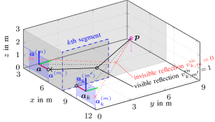
Figure 1: Visualization of a generic system setup, including a BS-PLA at position $\bm{a}$, an exemplary mirror PLA $\bm{a}_{k}$, and a UE at position $\bm{p}$. Exemplary multipath components corresponding to a wall segment of a limited extent are included, showing the resulting geometric visibility via ray-tracing.

An illustration of the system is given in Fig. 1, containing a single PLA representing a CSP at position $\bm{a}=[a_{x},a_{y},a_{z}]^{\mathsf{T}}$ that receives the signal from a single UE at location $\bm{p}=[p_{x},p_{y},p_{z}]^{\mathsf{T}}$ equipped with a single antenna. The PLA is equipped with $M$ antenna elements at locations $\bm{a}^{(m)}=[a_{x}^{(m)},a_{y}^{(m)},a_{z}^{(m)}]^{\mathsf{T}}$, defined relative to the reference point $\bm{a}$. The orientation of the PLA is known in the global coordinate system, with the orientation axes indicated as red, green, and blue lines. To model deterministic, also termed specular, multipath propagation, we employ a mirror source model [11] to model reflecting surfaces. An exemplary mirror source located at $\bm{a}_{k}$ with array elements at $\bm{a}_{k}^{(m)}$ (relative to $\bm{a}_{k}$) is included, obtained my mirroring the PLA at wall segment $k$ (dashed blue). Note that the orientation at the mirror PLA is mirrored. Considering a limited extent of the wall segment, not all array elements $m$ will receive a corresponding specular MPC, indicated for array elements $m$ and $m^{\prime}$ at the outer edges of the PLA. The following section briefly outlines a signal model that accounts for the varying visibility.

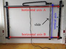
(a) wall mounted mechanical positioner

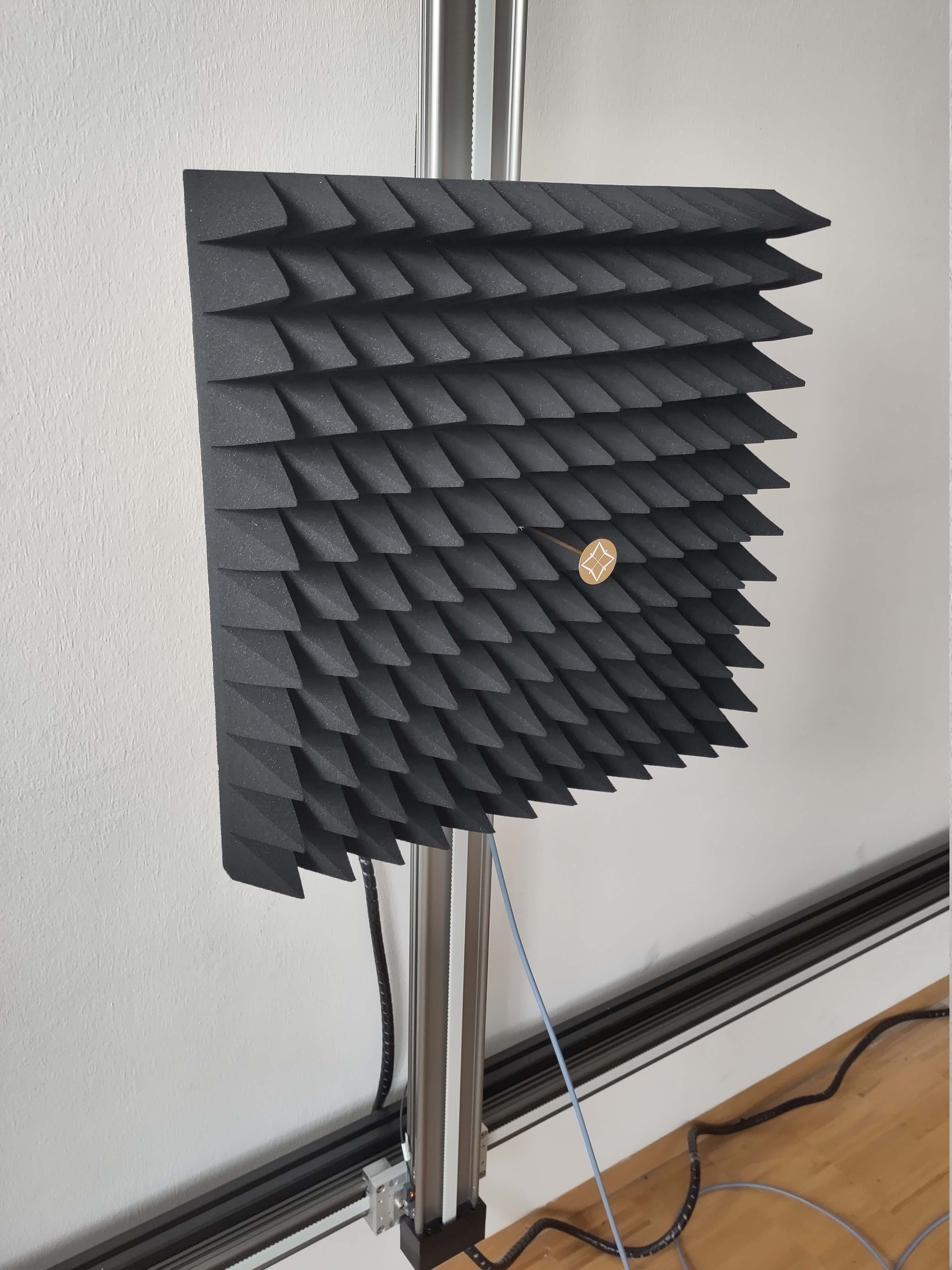
(b) antenna and absorber

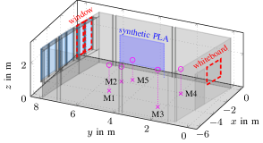
(c) medium sized environment (lab/office room)

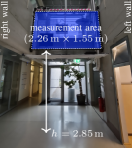
(d) PLA, photo A in LABEL:sub@fig:env:corridor

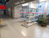
(e) UE region, photo B in LABEL:sub@fig:env:corridor

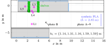
(f) large sized environment (corridor)

Figure 2: Visualization of measurement locations in medium and large size environments. (a) points distributed in medium size environment, (b) trajectory including obstruction in medium size environment, (c) distributed points and trajectory in large size environment.

The signal model includes specular MPCs as well as scattering and diffuse propagation in the environment. At each frequency, the received signal vector $\bm{y}(f)$ for a baseband frequency $f$ is denoted by

$$\bm{y}(f) =\sum_{k=1}^{K}\bm{h}_{k}(f)s(f)+\bm{w}_{\text{s}}(f)+\bm{w}(f)\in\mathbb{C}^{M}$$ (1)

consisting of a deterministic signal component in the form of a (finite) sum of $K$ MPCs attributable to specific environment features, a stochastic signal component $\bm{w}_{\text{s}}$ and additive white Gaussian noise (AWGN) $\bm{w}(f)$, representing the . The latter represents the sampled receiver noise, plus the a stochastic signal-related component denoted by $\bm{w}_{\text{s}}$. The stochastic signal-related component in $\bm{w}_{\text{s}}$ is commonly used to represent any form of stochastic multipath propagation such as scattering [12, 9] or a dense multipath component [13, 14, 15].

In the deterministic signal component, each MPC $k$ is described by the channel vector $\bm{h}_{k}(f)\in\mathbb{C}^{M}$ and the known transmit signal ${s}(f)$ in complex baseband. In realistic environments, the number of MPCs $K$ is unknown and varies depending on the locations of the transmitting and receiving devices. The entries of the channel vector are defined as [16]

$$[\bm{h}_{k}(f)]_{m}={\alpha}_{k,m}\mathrm{exp}(-j2\pi(f+f_{\mathrm{c}})\tau_{k,m})$$ (2)

with carrier frequency $f_{\mathrm{c}}$, MPC delay $\tau_{k,m}=\|\bm{a}^{(m)}_{k}-\bm{p}\|/c$, speed of light $c$, and the MPC amplitudes ${\alpha}_{k,m}$ defined as

$${\alpha}_{k,m} \propto\frac{\tilde{\alpha}_{k,m}b(\varphi_{k,m},\theta_{k,m})}{c\tau_{k,m}}v^{\text{vis}}_{k,m}.$$ (3)

The factor $b(\varphi,\theta)\in\mathbb{C}$ represents the complex-valued antenna gain pattern in direction of the azimuth $\varphi$ and elevation $\theta$ of the corresponding MPC at the $m$th array element. The quantity $\tilde{\alpha}_{k,m}$ on the right-hand side of (3) represents the environment-related, path loss compensated MPC amplitude, i.e., the amplitude related to transmit power and attenuation due to reflection at different materials. Note that for a specific MPC $k$, the amplitude $\tilde{\alpha}_{k,m}$ can vary per array element, e.g., due to angle dependent reflection coefficients of surfaces and their electromagnetic material properties, or when the size of the array becomes large, such that classical array processing assumptions such as plane wave propagation and negligible propagation attenuation along the array do not apply to the full PLA. The visibility is considered by the factor $v^{\text{vis}}_{k,m}$, which is $v^{\text{vis}}_{k,m}=1$ if the component $k$ is visible at array element $m$, and $v^{\text{vis}}_{k,m}=0$ otherwise. Note that this factor can be absorbed into the amplitudes but is expressed here to highlight the relation to the environment.

III Measurement System

The developed measurement system for synthetic PLAs consists of a mechanical positioner allowing to form 2-dimensional arrays with arbitrary planar geometry and a Rohde & Schwarz ZVA24 vector network analyzer (VNA) equipped with UWB antennas for performing the channel measurements.

RF hardware and antennas

The VNA covers a frequency range of $24\text{\,}\mathrm{GHz}$ (from DC) and was calibrated with a through-open-short-match (TOSM) calibration kit. The antennas used in the measurements are dipole antennas, manufactured from cent coins (see [17, App. B.3]), and dipole-slot antennas that were manufactured according to the XETS-antenna design from [18]. While the VNA covers a wider frequency range, measurements are only performed in the frequency band of $3-10\,\mathrm{GHz}$ for which the antennas are designed. Due to the measurement aperture allowing reception from azimuth and elevation, the slot antennas’ design was chosen as it exhibits an approximately omnidirectional pattern. When mounted on the absorber and reflector plate construction, the antennas only receive from the half-space facing away from the absorber.

Mechanical positioner

The mechanical positioner allows to form arbitrary planar synthetic array geometries in an automated fashion with sub-millimeter accuracy for the relative antenna positions. The maximum measurement area that can be used spans roughly $2.5\,\mathrm{m}\times 1.5\,\mathrm{m}$, shown in Fig. 2a. The horizontal and vertical axes are equipped with a dryve^® D1 motor controller driving two drylin^® NEMA24 stepper motors, allowing motion with variable acceleration, deceleration, and velocity. Each stepper motor has a holding break to keep the position during stop intervals. The vertical axis is equipped with a slide to mount the antennas and is itself attached to the horizontal axes. To emulate a PLA mounted directly on a surface, e.g., a CSP in a RW system, the mechanical positioner is equipped with a wideband absorber and a reflector plate on the slide behind the antenna (see Fig. 2b), removing the reflection from the surface on which the positioner is mounted on. Due to this construction, the distance from the antenna phase center to the back wall is roughly $43\text{\,}\mathrm{cm}$ (including the antenna length of $10\text{\,}\mathrm{cm}$).

Measurement environments

Measurements were performed in two environments of different sizes: in a medium size room representing a typical lab/office environment and in a large environment with a high ceiling and larger surfaces. Photos of measurement regions of the PLAs are shown in Fig. 2a and 2d. The number of array elements per PLA were $(112\times 75)$ and $(88\times 32)$, forming uniform rectangular arrays (URAs) with $\lambda/2$-spacing at $f_{\mathrm{c}}=$6.95\text{\,}\mathrm{GHz}$$ and $f_{\mathrm{c}}=$6\text{\,}\mathrm{GHz}$$ in the medium and large environments, respectively, with $\lambda=c/f_{\text{c}}$ denoting the wavelength. In each environment, measurements at five UE positions have been conducted, which are labeled Mx and Lx with antenna heights of $h_{\text{M}}=\{1.546,0.895,2.235,1.478,1.202\}\,\mathrm{m}$ and $h_{\text{L}}=\{1.145,1.317,1.162,1.590,1.592\}\,\mathrm{m}$, respectively. To aid the measurement analysis, 3-dimensional models were generated for both environments, shown in Fig. 2c and 2f for medium and large size, respectively. These allow to make use of the mirror source model to represent the MPCs from (1). The use of a mirror source model is widespread in literature [11], and in the context of this work enables to compare the model-based component visibility, with estimated components obtained by position-based beamforming or a super-resolution channel estimation algorithm.

IV Measurement Results and Analysis

TABLE I: Channel estimation results for all measurement positions in both measurement environments (see Fig. 2), using subarrays of size $(4\times 4)$ and a bandwidth of $500\text{\,}\mathrm{MHz}$.

	component energy in % of received signal energy (as mean $\pm$ std.dev.)
component	M1	M2	M3	M4	M5	L1	L2	L3	L4	L5
strongest	85.8 $\pm$ 6.5	76.5 $\pm$ 15.3	67.2 $\pm$ 9.4	43.3 $\pm$ 14.6	85.4 $\pm$ 17.5	42.4 $\pm$ 11.5	26.4 $\pm$ 9.0	12.7 $\pm$ 7.0	25.6 $\pm$ 6.5	9.3 $\pm$ 3.8
2nd strong.	3.9 $\pm$ 1.9	4.7 $\pm$ 4.6	9.7 $\pm$ 5.4	16.1 $\pm$ 8.2	6.7 $\pm$ 9.5	24.0 $\pm$ 7.9	12.3 $\pm$ 4.9	6.4 $\pm$ 2.5	17.2 $\pm$ 4.2	5.5 $\pm$ 2.1
3rd	2.1 $\pm$ 1.3	1.4 $\pm$ 1.3	3.9 $\pm$ 2.3	6.7 $\pm$ 4.1	1.2 $\pm$ 1.5	8.5 $\pm$ 3.8	7.7 $\pm$ 3.0	4.3 $\pm$ 1.6	11.8 $\pm$ 3.5	3.6 $\pm$ 1.2
4th	1.1 $\pm$ 0.6	0.7 $\pm$ 0.7	2.4 $\pm$ 1.0	4.2 $\pm$ 1.9	0.6 $\pm$ 0.6	4.5 $\pm$ 2.4	4.8 $\pm$ 1.7	3.3 $\pm$ 1.3	7.2 $\pm$ 3.6	2.6 $\pm$ 0.8
5th	0.8 $\pm$ 0.3	0.5 $\pm$ 0.4	1.8 $\pm$ 0.7	3.1 $\pm$ 1.3	0.4 $\pm$ 0.4	2.2 $\pm$ 1.2	3.4 $\pm$ 1.6	2.6 $\pm$ 0.9	3.6 $\pm$ 1.7	2.0 $\pm$ 0.6
6th	0.6 $\pm$ 0.3	0.4 $\pm$ 0.3	1.3 $\pm$ 0.5	2.4 $\pm$ 0.9	0.3 $\pm$ 0.3	1.3 $\pm$ 0.7	2.3 $\pm$ 1.0	2.0 $\pm$ 0.7	2.3 $\pm$ 1.1	1.7 $\pm$ 0.5
$\sum$ over 20	96.5 $\pm$ 1.1	97.8 $\pm$ 1.6	91.1 $\pm$ 2.8	82.3 $\pm$ 4.7	97.8 $\pm$ 1.7	87.0 $\pm$ 3.6	63.1 $\pm$ 7.1	38.4 $\pm$ 8.9	69.7 $\pm$ 6.3	31.8 $\pm$ 6.7
residual	3.1 $\pm$ 1.0	1.9 $\pm$ 1.4	7.9 $\pm$ 2.6	15.9 $\pm$ 4.2	1.9 $\pm$ 1.5	12.3 $\pm$ 3.4	35.3 $\pm$ 6.8	60.9 $\pm$ 15.3	29.0 $\pm$ 6.1	65.4 $\pm$ 6.5

This section presents the results from the performed measurement analysis and summarizes the results for the models in (1), (2) and (3). For the processing of measurements, we compare non-parametric and parametric approaches, both aided by a mirror source model based on the environment models (see Fig. 2). The non-parametric approach is a standard spherical wave beamformer, computed for the entire array and a bandwidth of $3\text{\,}\mathrm{GHz}$. The parametric approach is a super-resolution sparse Bayesian learning (SBL) algorithm to estimate MPCs, based on [19]. For processing the measurements with the SBL algorithm, a bandwidth of $500\text{\,}\mathrm{MHz}$ is used and the PLA is separated into subarrays of size ($4\times 4$) or ($8\times 8$). This allows to make use of the plane-wave assumption per subarray and to analyse the MPC visibility and amplitudes.

IV-A Spherical wave beamforming

An exemplary spherical beamformer spectrum computed for position M1 is shown in Fig. 3 in terms of the marginal spectra for combinations of delay, azimuth, and elevation. The azimuth-elevation power spectrum in Fig. 3a represents the view from the PLA shown in Fig. 2c. The azimuth-elevation spectrum in Fig. 3a shows a number of specular MPCs in addition to diffuse components. The azimuth-delay and elevation-delay spectra show similar combinations of specular and diffuse components. Locations of high power in the full spectrum represent locations of origin of specular MPCs from (2), i.e., of the corresponding mirror sources. A downside of the use of the full array for spherical beamforming is that the visibility information of MPCs is lost, with partially visible MPCs simply resulting in lower power at the corresponding spectrum bin.

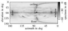
(a) az.-el. spectrum

(b) az.-dist. spectrum

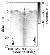
(c) el.-dist. spectrum

Figure 3: Spherical wave beamformer spectra for position M1 in the medium size environment using the full data (full bandwidth, all array elements). The azimuth-elevation power spectrum (Fig. 3a) represents the view from the synthetic PLA into the room (see Fig. 2c).

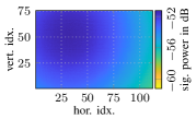
(a) direct path

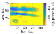
(b) window component

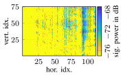
(c) whiteboard component

Figure 4: Signal power for each antenna position (e.g., PLA element) computed by performing position-based, i.e., spherical wave, beamforming for the direct path, window, and whiteboard reflections at the example of position M1. The (image) source positions are computed from the model in Fig. 2c.

IV-B Geometry-based analysis

By exploiting the known measurement position in combination with the environment model (at the example of position M1), the received power per-array element is computed to show local variations over the area of the PLA. Results are shown in Fig. 4 for three components: the direct path, the window reflection, and the whiteboard reflection, with the corresponding environment segments highlighted by red, dashed outlines in Fig. 2c. The direct path amplitudes in Fig. 4a show the expected attenuation due to the distance-dependent path loss and the gain pattern of the antenna. As patch antennas were used at the PLA and the UE, the gain pattern affects the amplitudes twice. The full PLA is in line-of-sight (LoS) condition with respect to the direct path. The window component (see Fig. 4b) shows much stronger amplitude variations and a distinct visibility region. The whiteboard component (see Fig. 4c) shows significant amplitude fading, which relates to the computed geometric visibility regions (c.f. Fig. 5d).

IV-C Super-resolution channel estimation

For the parametric analysis, the SBL algorithm [19] is applied to the signals per subarray. This allows to make use of the plane wave assumption and assume negligible propagation attenuation along the subarrays [16], due to the small subarray size w.r.t. the propagation distance to modify (1) accordingly. Furthermore, components are assumed to be visible for all subarray elements, using square URAs with $M=\{16,64\}$ array elements. Increasing $M$ improves the analysis of the component visibility due to the array gain, e.g., compared to the results from Sec. IV-B. We restrict the maximum number of components to be estimated in the SBL-algorithm to $\hat{K}=20$ to reduce the computation time.

IV-C1 Model representation

A summary of the SBL-estimates for the measurement positions in both environments is given in Table I. The table compares the estimated component energy (as a percentage of the total received signal energy) for the six strongest components at all measurement positions. The results are shown in terms of mean and standard deviation taken over the resulting $N_{\text{s}}=500$ subarrays. Comparing the total estimated energy with the residual energy gives a metric on how well the channel estimator captures the total signal energy. The results for different measurement positions show that a high percentage of the signal energy is covered by all estimated components, with usually close to $95\text{\,}\mathrm{\char 37\relax}$ energy contained in all estimated components in the medium environment. In the large environment, the fixed number of $K=20$ components is not sufficient, capturing usually below $80\text{\,}\mathrm{\char 37\relax}$ or the signal energy. The significantly lower percentage of $82\text{\,}\mathrm{\char 37\relax}$ for M4 can be explained by the proximity to metal shelves, from which a larger number of scattered components can be expected, resulting in more diffuse components not well represented by the deterministic MPC model. Similarly, locations L3 and L5 which experience strong obstructions due to the metal shelves only capture below $40\text{\,}\mathrm{\char 37\relax}$ of the total signal energy on average, which is also attributable to a larger number of diffuse components not well represented by the model.

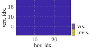
(a) direct path model vis. ($4\times 4$)

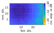
(b) direct path amp. est. ($4\times 4$)

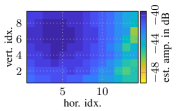
(c) direct path amp. est. ($8\times 8$)

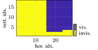
(d) whiteboard path model vis. ($4\times 4$)

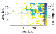
(e) whiteboard path amp. est. ($4\times 4$)

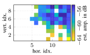
(f) whiteboard path amp. est. ($8\times 8$)

Figure 5: Estimated amplitudes obtained with the SBL-algorithm [19] for $(4\times 4)$ and $(8\times 8)$ subarrays and 500 MHz bandwidth. Data association is performed for direct path and whiteboard components.

IV-C2 Component visibility

To analyze the visibility and spatial amplitude distribution of estimated components, we rely on the environment models shown in Fig. 2f and 2f to compute image source positions for expected MPCs. For each subarray, the estimates obtained from the SBL-algorithm (component delay, azimuth, and elevation) are associated with the components corresponding to the computed image sources using the data association (DA) algorithm from [20].

Medium environment

The estimated amplitudes per subarray associated with modeled components are shown alongside the computed geometric visibility using the model (and ray tracing) in Fig. 5, shown by the example of M1 and selected components. The direct path is visible at all subarrays independent of their size, showing a similar distribution of estimated amplitudes (see Fig. 5b and 5c). The combined effect of the antenna gain patterns is again observable, with the shown estimated amplitudes compensated for the distance-dependent path loss. The whiteboard component is only visible in a rectangular area in the upper right corner of the full array (see Figure 5d), which represents the subarray regions where components were found that could be associated to the corresponding image source. The differences between small and large subarray size in Fig. 5e and 5f can be attributed to the increased array gain of the larger ones, as components with lower signal-to-noise ratio (SNR) can be detected.

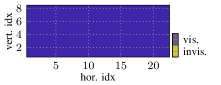
(a) direct path model vis. ($4\times 4$)

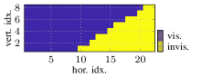
(b) right wall path model vis.

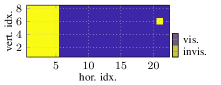
(c) left wall path model vis. ($4\times 4$)

(d) direct path amp. est. ($4\times 4$)

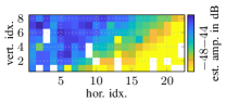
(e) right wall path amp. est. ($4\times 4$)

(f) left wall path amp. est. ($4\times 4$)

Figure 6: Estimated amplitudes obtained with the SBL-algorithm from [19] for the large environment at position L1. Subarrays of size $(4\times 4)$ are used with $500~{}\mathrm{MHz}$ bandwidth, comparing two first order reflections.

Large environment

Similar results are obtained for the large-sized environment. At the example of measurement position L1, Fig. 6 shows the results for subarrays of dimension $(4\times 4)$ and a bandwidth of $500\text{\,}\mathrm{MHz}$. Note that the measurement area is smaller due to the position in the environment. Additionally, the lower carrier frequency of $f_{\text{c}}=$6\text{\,}\mathrm{GHz}$$ results in a slightly larger inter-element spacing. The figure shows the computed visibility (top row of subplots) and the amplitude estimates obtained with the SBL algorithm (bottom row) for the direct path, and the walls to the left and right of the array (as seen from the array).

The direct path (Fig. 6a and 6d) is generally in LoS condition for the full PLA area. Nonetheless, variations in the estimated amplitude can be observed, which are likely caused by overlap between the left wall component (see the model in Fig. 2f and photo in 2d), as the $(4\times 4)$ URAs have a comparably low spatial resolution. For the reflection via the right wall (Figure 6b and 6e), the visibility computed from the environment model shows a triangular region of component invisibility in the bottom right corner of the PLA, which coincides with the region of low estimated amplitudes of similar shape. Note that the geometric shape of the visibility region is due to the measurement area located underneath the right wall (see Fig. 2e), with the lower wall edge representing the boundary between the visibility regions for the corresponding MPC. The left wall, in turn, shows stronger amplitude fading and less clear correspondence with the computed geometric visibility. Again, these variations could be attributed to the geometric configuration of the measurement setup: as the measurement location is close to the corresponding image source, path overlap in the delay and the angle domain again likely causes fading.

V Conclusion and Future Work

The synthetic PLA measurements and the analysis presented in this paper have shown the feasibility and necessity of employing visibility regions for MPC-based models in the context of PLAs. Based on the channel measurements, we have shown that it is possible to perform super-resolution channel estimation for subarrays for which local stationarity can be assumed, inherently accounting for visibility. This is important in location-aware applications, where the measured channel is used to estimate the user location or infer environment parameters. Consequently, robust algorithms must consider the limited component visibility and varying number of components and received signal power.

Future work will deal with algorithms that exploit the described propagation conditions as well as refinement of the outlined channel model that considers visibility on a per-array, or at least per-subarray level. Furthermore, algorithms for the optimal fusion of local measurements/estimates obtained by subarrays to attain the performance of a corresponding fully coherent PLA aperture are under development based on the channel measurements.

References

- [1] D. W. M. Guerra and T. Abrão, “Clustered double-scattering channel modeling for XL-MIMO with uniform arrays,” IEEE Access, vol. 10, pp. 20 173–20 186, Feb. 2022.
- [2] Z. H. Shaik, E. Björnson, and E. G. Larsson, “Mmse-optimal sequential processing for cell-free massive mimo with radio stripes,” IEEE Trans. Commun., vol. 69, no. 11, pp. 7775–7789, 2021.
- [3] D. Dardari, “Communicating with large intelligent surfaces: Fundamental limits and models,” IEEE J. Sel. Areas Commun., vol. 38, no. 11, pp. 2526–2537, 2020.
- [4] E. Björnson, H. Wymeersch, B. Matthiesen, P. Popovski, L. Sanguinetti, and E. de Carvalho, “Reconfigurable intelligent surfaces: A signal processing perspective with wireless applications,” IEEE Signal Process. Mag., vol. 39, no. 2, pp. 135–158, 2022.
- [5] L. Van der Perre, E. G. Larsson, F. Tufvesson, L. De Strycker, E. Björnson, and O. Edfors, “RadioWeaves for efficient connectivity: analysis and impact of constraints in actual deployments,” in 2019 53rd Asilomar Conference on Signals, Systems, and Computers. IEEE, nov 2019, pp. 15–22.
- [6] J. F. Esteban and M. Truskaller, “Use case-driven specifications and technical requirements and initial channel model,” REINDEER project, Deliverable ICT-52-2020 / D1.1, Sep. 2021.
- [7] X. Gao, F. Tufvesson, and O. Edfors, “Massive mimo channels - measurements and models,” in 2013 Asilomar Conference on Signals, Systems and Computers, 2013, pp. 280–284.
- [8] E. D. Carvalho, A. Ali, A. Amiri, M. Angjelichinoski, and R. W. Heath, “Non-stationarities in extra-large-scale massive mimo,” IEEE Wireless Communications, vol. 27, no. 4, pp. 74–80, 2020.
- [9] J. Flordelis, X. Li, O. Edfors, and F. Tufvesson, “Massive MIMO extensions to the COST 2100 channel model: Modeling and validation,” IEEE Trans. Wireless Commun., vol. 19, no. 1, pp. 380–394, Oct. 2020.
- [10] H. Chen, A. Elzanaty, R. Ghazalian, M. F. Keskin, R. Jäntti, and H. Wymeersch, “Channel model mismatch analysis for xl-MIMO systems from a localization perspective,” 2022. [Online]. Available: https://arxiv.org/abs/2205.15417
- [11] T. Pedersen, “Modeling of path arrival rate for in-room radio channels with directive antennas,” IEEE Trans. Antennas Propag., vol. 66, no. 9, pp. 4791–4805, 2018.
- [12] F. M. Schubert, M. L. Jakobsen, and B. H. Fleury, “Non-stationary propagation model for scattering volumes with an application to the rural LMS channel,” IEEE Trans. Antennas Propag., vol. 61, no. 5, pp. 2817–2828, 2013.
- [13] A. Richter, “Estimation of Radio Channel Parameters: Models and Algorithms,” Ph.D. dissertation, Ilmenau University of Technology, 2005.
- [14] J. Salmi, A. Richter, and V. Koivunen, “Detection and tracking of MIMO propagation path parameters using state-space approach,” IEEE Trans. Signal Process., vol. 57, no. 4, pp. 1538–1550, Apr. 2009.
- [15] E. Leitinger, P. Meissner, C. Rudisser, G. Dumphart, and K. Witrisal, “Evaluation of position-related information in multipath components for indoor positioning,” IEEE J. Sel. Areas Commun., vol. 33, no. 11, pp. 2313–2328, Nov. 2015.
- [16] D. H. Johnson and D. E. Dudgeon, Array signal processing: concepts and techniques. Simon & Schuster, Inc., 1992.
- [17] C. Krall, “Signal processing for ultra wideband transceivers,” Ph.D. dissertation, Graz University of Technology, 2008.
- [18] J. R. Costa, C. R. Medeiros, and C. A. Fernandes, “Performance of a crossed exponentially tapered slot antenna for uwb systems,” IEEE Trans. Antennas Propag., vol. 57, no. 5, pp. 1345–1352, 2009.
- [19] T. L. Hansen, M. A. Badiu, B. H. Fleury, and B. D. Rao, “A sparse Bayesian learning algorithm with dictionary parameter estimation,” in 2014 IEEE 8th Sensor Array and Multichannel Signal Processing Workshop (SAM). IEEE, 2014, pp. 385–388.
- [20] P. Meissner, E. Leitinger, M. Fröhle, and K. Witrisal, “Accurate and robust indoor localization systems using ultra-wideband signals,” arXiv preprint arXiv:1304.7928, 2013.