Scalable Demand-Driven Call Graph Generation for Python

Abstract.

Call graph generation is the foundation of inter-procedural static analysis. PyCG is the state-of-the-art approach for generating call graphs for Python programs. Unfortunately, PyCG does not scale to large programs when adapted to whole-program analysis where dependent libraries are also analyzed. Further, PyCG does not support demand-driven analysis where only the reachable functions from given entry functions are analyzed. Moreover, PyCG is flow-insensitive and does not fully support Python’s features, hindering its accuracy.

To overcome these drawbacks, we propose a scalable demand-driven approach for generating call graphs for Python programs, and implement it as a prototype tool Jarvis. Jarvis maintains an assignment graph (i.e., points-to relations between program identifiers) for each function in a program to allow reuse and improve scalability. Given a set of entry functions as the demands, Jarvis generates the call graph on-the-fly, where flow-sensitive intra-procedural analysis and inter-procedural analysis are conducted in turn. Our evaluation on a micro-benchmark of 135 small Python programs and a macro-benchmark of 6 real-world Python applications has demonstrated that Jarvis can significantly improve PyCG by at least 67% faster in time, 84% higher in precision, and at least 10% higher in recall.

1. Introduction

Python has become one of the most popular programming languages in recent years (TIOBE, 2023). The prevalent adoption of Python in a variety of application domains calls for great needs of static analysis to ensure software quality. Call graph generation is the foundation of inter-procedural static analysis. It embraces a wide scope of static analysis tasks, e.g., security analysis (Barros et al., 2015; Chess and McGraw, 2004; Livshits and Lam, 2005; Guarnieri and Livshits, 2009), dependency management (Hejderup et al., 2018; Santos et al., 2022; Huang et al., 2022) and software debloating (Quach et al., 2018; Bruce et al., 2020).

It is challenging to generate a precise and sound call graph for Python. Python has dynamic language features as any interpreted language does, which makes the analysis more complicated compared with compiled languages (Jensen et al., 2009; Nagy et al., 2021; Nielsen et al., 2021). For example, dynamically typed variables demand the analysis to undertake a precise inter-procedural points-to analysis to resolve the type of variables. Several approaches, i.e., Pyan (Fraser et al., 2019), Depends (Zhang and Jin, 2018) and PyCG (Salis et al., 2021), have been recently proposed to generate call graphs for Python programs. Specifically, PyCG is the state-of-the-art, which achieves the best precision, recall, and time and memory performance (Salis et al., 2021). It conducts a flow-insensitive inter-procedural points-to analysis using a fixed-point algorithm. This algorithm takes unfixed iterations to update an assignment graph (i.e., points-to relations between program identifiers) until it is unchanged. After the assignment graph for the whole program is constructed, the call graph is generated.

However, PyCG still suffers several drawbacks. First, PyCG conducts an exhaustive analysis on the application program only without analyzing any dependent library (i.e., as showed by the left part of Fig. 1). As a result, the generated call graph is infeasible for static analysis tasks such as dependency management (Hejderup et al., 2018; Santos et al., 2022; Huang et al., 2022) and software debloating (Quach et al., 2018; Bruce et al., 2020) where the calls into directly and transitively dependent libraries are needed. We adapt PyCG to whole-program analysis by further analyzing all dependent libraries (as showed by the middle part of Fig. 1), but find that it does not scale to large programs that usually have many dependent libraries.

Second, due to the intrinsic design of its exhaustive analysis, PyCG does not support demand-driven analysis which only analyzes the reachable functions from a set of given entry functions (i.e., the demands) rather than analyzing all functions (i.e., as illustrated by the right part of Fig. 1). However, demand-driven analysis is needed for static analysis tasks such as dependency management (Hejderup et al., 2018; Santos et al., 2022; Huang et al., 2022) and software debloating (Quach et al., 2018; Bruce et al., 2020). A workaround to achieve demand-driven analysis is to prune the call graph generated by PyCG according to the given entry functions, but it wastes computation time on analyzing unreachable functions and suffers the scalability issue.

Third, PyCG conducts a flow-insensitive analysis which ignores control flows and over-approximately computes points-to relations. This over-approximation introduces false positives. In addition, PyCG introduces false negatives because it does not fully support Python’s language features (e.g., built-in types and functions).

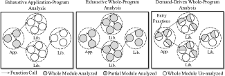
Figure 1. Analysis Scope of Call Graph Generation

To overcome these drawbacks, we propose a scalable demand-driven call graph generation approach for Python, and implement it as a prototype tool Jarvis. Jarvis has four key characteristics which are different from PyCG. First, Jarvis is scalable to large programs as it maintains an assignment graph for each function in a program. Such a design allows Jarvis to reuse the assignment graph of a function without reevaluating the function at each call site. Second, Jarvis generates call graphs on-the-fly, i.e., it uses the intermediate assignment graph before the call site to infer the callee function. Therefore, Jarvis inherently supports customized analysis scope (e.g., application-program, whole-program, or any intermediate scope). Third, Jarvis is demand-driven. Given a set of entry functions as the demands, Jarvis only analyzes the reachable functions from the entry functions. Therefore, unnecessary computation for un-demanded functions is skipped. Fourth, Jarvis is flow-sensitive to improve its precision. It creates a copy of assignment graph when control flow diverges in a function, and merges assignment graphs when control flow converges. Besides, Jarvis supports Python’s language features more comprehensively, which helps to improve its recall.

We evaluate the efficiency and effectiveness of Jarvis on a micro-benchmark of 135 small Python programs (covering a wide range of language features) and a macro-benchmark of 6 real-world Python applications. For efficiency, Jarvis improves PyCG by at least 67% faster in time in the scenario of exhaustive whole-program analysis; and Jarvis takes averagely 3.84 seconds for 2.8k lines of application code in the scenario of demand-driven whole-program analysis. For effectiveness, Jarvis improves PyCG by 84% in precision and at least 10% in recall in demand-driven whole-program analysis.

In summary, this work makes the following contributions.

• We proposed Jarvis to scalably generate call graphs for Python programs on demand via flow-sensitive on-the-fly analysis.

• We conducted experiments on two benchmarks to demonstrate the improved efficiency and effectiveness over the state-of-the-art.

2. Background

We first introduce the assignment graph in PyCG and then discuss the drawbacks of PyCG using a motivating example.

2.1. Assignment Graph in PyCG

As Python has higher-order functions, module imports and object-oriented programming features, the assignment graph in PyCG maintains the assignment relations between program identifiers, i.e., variables, functions, classes and modules. It has a broader scope than a traditional points-to graph by further including functions, classes and modules. PyCG uses a fixed-point algorithm to iteratively update the assignment graph by resolving unknown identifiers until the assignment graph is fixed. After it constructs the assignment graph for a Python program, it utilizes the assignment graph to generate the call graph by resolving all calls to potentially invoked functions.

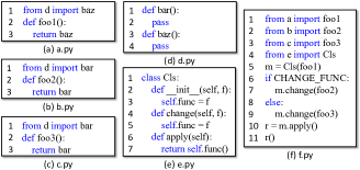
Figure 2. A Motivating Example

2.2. Drawbacks of PyCG

To illustrate the drawbacks of PyCG, we use a motivating example, as shown in Fig. 2, which consists of six modules (i.e., files). PyCG takes four iterations to construct the assignment graph, as shown in Fig. 3. Specifically, the first iteration parses imports, class, functions, returns, assignment, etc. for updating the assignment graph (corresponding to the black ovals and arrows in Fig. 3). For the import at Line 1 in f.py, PyCG adds a points-to relation f.foo1 $\xrightarrow{}$ a.foo1, meaning that function foo1 in module f is function foo1 in module a. For class creation and assignment at Line 5 in f.py, PyCG adds a points-to relation f.m $\xrightarrow{}$ f.Cls, denoting that variable m in module f is an instance of class f.Cls. Similarly, for each function in class Cls in e.py, variable self is created and points to class e.Cls (e.g., e.Cls.apply.self $\xrightarrow{}$ e.Cls). For the return at Line 3 in a.py, virtual variable ret is added and points to a.baz (i.e., a.foo1.<ret> $\xrightarrow{}$ a.baz), meaning that the return of function foo1 in module a points to the function baz in module a. At the first iteration, PyCG does not utilize the points-to relations in the assignment graph. Thus, the invoking variable (e.g., f.m) and the function definition for function call (e.g., f.m.change) is unknown yet.

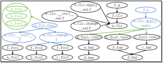
Figure 3. Assignment Graph for PyCG

At the following iterations, PyCG computes the transitive closure of the assignment graph, applies simplifications (Fahndrich and Aiken, 1996) and updates the assignment graph. At the second iteration (corresponding to the blue ovals and arrows in Fig. 3), PyCG resolves the function calls at Line 7 and 9 in f.py to e.Cls.change using the points-to relation f.m $\xrightarrow{}$ e.Cls, and thus two points-to relations e.Cls.change.f $\xrightarrow{}$ f.foo2 and e.Cls.change.f $\xrightarrow{}$ f.foo3 are added. Similarly, the function call at Line 10 in f.py is resolved to e.Cls.apply, and hence variable f.r is added and points to the virtual variable of the return of e.Cls.apply (i.e., f.r $\xrightarrow{}$ e.Cls.apply.<ret>).

At the third iteration (corresponding to the green ovals and arrows in Fig. 3), the pointed functions of e.Cls.func are collapsed into one set {a.foo1, b.foo2, c.foo3} for simplification and performance. Then, for the return at Line 7 in e.py, the return of these pointed functions are pointed to by the return of e.Cls.apply (e.g., e.Cls.apply.<ret> $\xrightarrow{}$ a.foo1.<ret>). At the fourth iteration, PyCG makes no changes to the assignment graph, and then starts to generate the call graph on the basis of the assignment graph.

As illustrated by the previous example, there are several drawbacks in PyCG’s call graph generation. PyCG undergoes several iterations to obtain a fixed assignment graph, and each module and function are analyzed in each iteration with no discrimination, causing unnecessary computation. Therefore, PyCG suffers the scalability issue and does not support demand-driven analysis. Moreover, PyCG conducts a flow-insensitive inter-procedural analysis, which introduces false positives. PyCG generates three calls from e.apply to a.foo1, b.foo2 and c.foo3. However, the call to a.foo1 is a false positive because PyCG disregards the flow of Line 5, 7 and 9 in f.py. Due to this false positive, PyCG introduces another false positive, i.e., the call from f.main to d.baz (here code fragment located in a module, e.g., Line 5–11 in f.py, is named main).

3. Approach

We first give notions and domains of our analysis. Then, we describe the overview of Jarvis. Finally, we elaborate Jarvis in detail.

3.1. Notions and Domains

Our analysis works on the AST representation of Python programs using the built-in ast library in Python. Identifiers are important elements in Python programs, and expressions are considered as the basic analysis block as it is atomic and can be composed into complicated program elements. Fig. 4 shows the basic notions used in our analysis. Specifically, each identifier definition $d$ is defined as a tuple $\langle\tau,\phi,n\rangle$, where $\tau$ denotes the identifier type, $\phi$ denotes the identifier namespace, and $n$ denotes the identifier name. $\tau$ can be one of the five types, i.e., module in the application (mod), module in external dependent libraries (ext_mod), class (cls), function (func), and variable (var). Each expression $e$ can be various types, and a full list of expressions can be found at the official Python website (Foundation, 2023).

$$d\in Def:: =\langle\tau,\phi,n\rangle$$

$$\tau\in IdentifierType:: =\textbf{mod}\mid\textbf{ext\_mod}\mid\textbf{cls}\mid\textbf{func}\mid\textbf{var}$$

$$n\in IdentifierName:: =the~{}set~{}of~{}program~{}identifier~{}names$$

$$\phi\in Namespace:: =(n,\tau)^{*}$$

$$e\in Expr:: =the~{}set~{}of~{}expressions$$

Figure 4. Notions of Our Analysis

Then, we introduce the six domains that are maintained in our analysis, i.e., function assignment graph, control flow graph, function summary, class summary, import summary, and call graph.

Function Assignment Graph ($\mathcal{FAG}$). A function assignment graph (FAG) maintains points-to relations of a function, which is different from the program-level assignment graph in PyCG. It is designed at the function level to allow reuse and improve scalability (see Sec. 3.3.2). Formally, a function assignment graph is denoted as a 3-tuple $\langle Def,{\color[rgb]{0,0,0}Expr},Pts\rangle$, where $Def$ denotes identifier definitions in a function, $Expr$ denotes expressions in a function, and $Pts$ denotes points-to relations between identifiers. Each points-to relation $pts\in Pts$ is denoted as a 3-tuple $\langle d_{1},d_{2},e\rangle$ (or $d_{1}\xrightarrow{e}d_{2}$), where $d_{1}$, $d_{2}$ $\in$ $Def$, and $e\in Expr$ denotes the evaluated expression that results in $pts$. Here $e$ facilitates flow-sensitive analysis (see Sec. 3.3.4).

Hereafter, we use $\mathcal{FAG}_{in}$ to denote the initial FAG before the evaluation of the first expression in a function, which contains points-to relations about parameter variables that are passed from its caller. We use $\mathcal{FAG}_{e}$ to denote the intermediate FAG after the expression $e$ is evaluated. We use $\mathcal{FAG}_{R}$ to denote the final FAG after all expressions are evaluated. We use $\mathcal{FAG}_{out}$ to denote the output FAG which contains the final points-to relations about parameter variables that will be passed back to its caller.

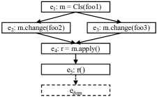
Figure 5. Control Flow Graph of f.main

Control Flow Graph ($\mathcal{CFG}$). The control flow graph of a function maintains the control dependencies between expressions. It is denoted as a 4-tuple $\langle{\color[rgb]{0,0,0}Expr},{\color[rgb]{0,0,0}Ctrl},{\color[rgb]{0,0,0}e_{en}},E_{r}\rangle$, where $Expr$ denotes expressions in a function, $Ctrl$ denotes control flows in a function, $e_{en}$ denotes the entry expression, and $E_{r}$ denotes the return expressions (either explicit returns or implicit returns). Each control flow $ctrl\in$ $Ctrl$ is denoted as a 2-tuple $\langle e_{1},e_{2}\rangle$, representing the control flow from expression $e_{1}$ to expression $e_{2}$. Notice that we add a virtual dummy expression $e_{dum}$ that all return expressions flow to.

Example 3.1.

The control flow graph of function f.main (i.e., Line 5-11 in f.py) in Fig. 2 is shown in Fig. 5. $Expr$ consists of six expressions, i.e., $e_{1}$, $e_{2}$, $e_{3}$, $e_{4}$, $e_{5}$ and $e_{dum}$. $e_{1}$ is the entry expression (i.e., $e_{en}=e_{1}$). $e_{5}$ is the only one return expression (i.e., $E_{r}=\{e_{5}\}$). $Ctrl$ contains $\langle e_{1},e_{2}\rangle$, $\langle e_{1},e_{3}\rangle$, $\langle e_{2},e_{4}\rangle$, $\langle e_{3},e_{4}\rangle$, $\langle e_{4},e_{5}\rangle$, $\langle e_{5},e_{dum}\rangle$.

Function Summary ($\mathcal{F}$). The function summary contains a set of functions that are visited in our analysis. Each function $f\in\mathcal{F}$ is denoted as a 2-tuple $\langle d,{\color[rgb]{0,0,0}P}\rangle$, where $d\in Def$ denotes the definition of $f$, and $P$ denotes the set of parameter names of $f$. Notice that code fragment located in a module, e.g., Line 5–11 in f.py in Fig. 2, is regarded as a virtual function, which is named main.

Class Summary ($\mathcal{C}$). The class summary is denoted as a 2-tuple $\langle{\color[rgb]{0,0,0}Hier},{\color[rgb]{0,0,0}Incl}\rangle$, where $Hier$ denotes class hierarchy (i.e., inheritance relations between classes), and $Incl$ denotes the inclusion relations from class to its included function definitions. Each entry in $Hier$ is denoted as a 2-tuple $\langle d_{clsb},$ $d_{clss}\rangle$, where $d_{clsb}$ and $d_{clss}\in$ $Def$ denote the base calss and sub class, respectively. Each entry in $Incl$ is denoted as a 2-tuple $\langle d_{c},d_{f}\rangle$, where $d_{c}\in Def$ denotes a class, and $d_{f}\in Def$ denotes a function definition in the class.

Import Summary ($\mathcal{I}$). The import summary contains points-to relations from importing definition to imported definition. Each entry in $\mathcal{I}$ is denoted as a 3-tuple $\langle{\color[rgb]{0,0,0}d_{s}},d_{t},e\rangle$, where $d_{s}\in Def$ denotes the importing definition, $d_{t}\in Def$ denotes the imported definition, and $e$ denotes the import expression. For example, for the import expression at Line 1 in f.py in Fig. 2, a.foo1 is the imported definition, and f.foo1 is the importing definition.

Call Graph ($\mathcal{CG}$). The call graph contains call relations in a program. It is denoted as a 2-tuple $\langle V,E\rangle$, where each entry in $E$ is denoted as a 2-tuple $\langle f_{er},f_{ee}\rangle$, representing a call relation from the caller function $f_{er}\in V\subseteq Def$ to the callee function $f_{ee}\in V$.

3.2. Overview of Jarvis

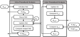
Figure 6. Approach Overview of Jarvis

The overview of Jarvis is shown in Fig. 6. Given an entry function, it first runs intra-procedural analysis on this function, and then runs inter-procedural analysis and intra-procedural analysis in turn.

Intra-Procedural Analysis. When running intra-procedural analysis on a function $f$, Jarvis takes as input $\theta_{call}$, which denotes the points-to relations about argument variables passed from the call expression $call$ that invokes $f$. For an entry function, its $\theta_{call}$ is empty by default. Jarvis takes four steps to complete intra-procedural analysis. First, Jarvis initializes $\mathcal{FAG}_{in}$ before evaluating the function’s expressions. Then, Jarvis reuses $\mathcal{FAG}_{out}$ if the function has been visited before and the points-to relations about argument variables are the same as before. Otherwise, Jarvis updates the FAG. It applies transfer function to evaluate each expression $e$ in the function, and adds the evaluation result $\Delta_{e}$ to obtain $\mathcal{FAG}_{e}$. Specifically, if $e$ is a call expression $call^{\prime}$, Jarvis runs inter-procedural analysis to obtain its evaluation result $\Delta_{call^{\prime}}$. Finally, after all expressions are evaluated, Jarvis computes $\mathcal{FAG}_{out}$, and passes $\mathcal{FAG}_{in}$ and $\mathcal{FAG}_{out}$ back to the inter-procedural analysis on $call$.

Inter-Procedural Analysis. Jarvis starts inter-procedural analysis when a call expression $call^{\prime}$ in $f$ is resolved into a callee function $f^{\prime}$. Specifically, Jarvis first creates a call relation $\langle f,f^{\prime}\rangle$ and updates it into the call graph. Then, Jarvis computes the points-to relations about argument variables in $call^{\prime}$ (i.e., $\theta_{call^{\prime}}$). Next, Jarvis runs intra-procedural analysis on $f^{\prime}$ using $\theta^{\prime}_{call}$, and passes $\mathcal{FAG}^{\prime}_{in}$ and $\mathcal{FAG}^{\prime}_{out}$ back. Finally, Jarvis computes the changed points-to relations about argument variables (i.e., $\Delta_{call^{\prime}}$) from $\mathcal{FAG}^{\prime}_{in}$ to $\mathcal{FAG}^{\prime}_{out}$, and passes $\Delta_{call^{\prime}}$ back to the intra-procedural analysis on $f$ in order to reflect the evaluation results from $call^{\prime}$.

After our intra-procedural analysis and inter-procedural analysis finish, we can directly obtain the demanded call graph because it is constructed on-the-fly in our inter-procedural analysis.

Algorithm 1 Intra-Procedural Analysis

1$f$, $\theta_{call}$

2$\mathcal{FAG}^{f}_{in}$, $\mathcal{FAG}^{f}_{out}$

3function intra_analysis

4     $g_{in}$ = computeParamPts($f.P$, $\theta_{call}$)

5     if $not$ isVisited($m_{f}$) then

6         $\mathcal{F},\mathcal{C},\mathcal{I}$ $\leftarrow$ previsitModule($m_{f}$)

7     end if

8     $g_{in}\leftarrow\mathcal{I}_{m_{f}}$

9     if isVisited($f$) and isEqual($g_{in}$, $\mathcal{FAG}^{f}_{in}$) then

10         return $\mathcal{FAG}^{f}_{in}$, $\mathcal{FAG}^{f}_{out}$

11     end if

12     $\mathcal{FAG}^{f}_{in}$ = $g_{in}$

13     for each $e\in$ preOrder(AST of $f$) do

14         for each $e.p\in$ parents of $e$ and outDegree($e.p$) $>1$ do

15              $\mathcal{FAG}^{f}_{e.p}$ = copy($\mathcal{FAG}^{f}_{e.p}$)

16         end for

17         if $e$ has one parent then

18              $\Delta_{e}$ = applyTransferRule($f$, $e$, $\mathcal{FAG}^{f}_{e.p}$)

19              $\mathcal{FAG}^{f}_{e}$ = updateFAG($\mathcal{FAG}^{f}_{e.p}$, $\Delta_{e}$, $e$)

20         end if

21         if $e$ has more than one parent then

22              $g_{merge}=\bigcup_{e.p\in parents~{}of~{}e}\mathcal{FAG}^{f}_{e.p}$

23              $\Delta_{e}$ = applyTransferRule$(f,e,g_{merge})$

24              $\mathcal{FAG}^{f}_{e}$ = updateFAG$(g_{merge},\Delta_{e},e)$

25         end if

26     end for

27     $\mathcal{FAG}^{f}_{R}=\bigcup_{e\in\mathcal{CFG}_{f}.E_{r}}\mathcal{FAG}^{f}_{e}$

28     setVisited($f$)

29     $\mathcal{FAG}^{f}_{out}$ = computeOutputFAG$(\mathcal{FAG}^{f}_{in},\mathcal{FAG}^{f}_{R})$

30     return $\mathcal{FAG}^{f}_{in}$, $\mathcal{FAG}^{f}_{out}$

31end function

3.3. Intra-Procedural Analysis

The algorithm of our intra-procedural analysis is presented in Alg. 1. It mainly consists of four steps, i.e., Initialize FAG, Reuse FAG, Update FAG, and Compute Output FAG.

3.3.1. Initialize FAG

Given the points-to relations $\theta_{call}$ about argument variables in the call expression $call$ that invokes function $f$, this step initializes $\mathcal{FAG}^{f}_{in}$ (Line 2–6 in Alg. 1), i.e., the initial FAG of $f$ before evaluating the first expression in $f$. First, it computes the points-to relations about parameter variables (i.e., $f.P$) according to $\theta_{call}$ based on the mapping between parameters and passed arguments, and puts the result to a temporary FAG $g_{in}$ (Line 2). Then, if the module $m_{f}$ where $f$ locates (which can be derived from $f.d.\phi$) has not been visited before, it updates $\mathcal{F}$, $\mathcal{C}$ and $\mathcal{I}$ by parsing the code of $m_{f}$ (Line 3–5). Finally, it adds the global points-to relations resulted from import expressions to $g_{in}$ (Line 6). Now $g_{in}$ is the initial FAG of $f$, and will be assigned to $\mathcal{FAG}^{f}_{in}$ (Line 10).

3.3.2. Reuse FAG

If the function has been visited before, the FAG of $f$ has been constructed, which provides the opportunity to reuse the FAG and improve scalability. To this end, this step first determines whether $f$ has been visited before (Line 7). If yes, it further determines whether $g_{in}$ equals to $\mathcal{FAG}_{in}^{f}$ that is constructed in the previous visit (Line 7). If yes (meaning that the FAG can be reused), it directly returns the previously constructed $\mathcal{FAG}_{in}^{f}$ and $\mathcal{FAG}_{out}^{f}$ (i.e., the final points-to relations about parameter variables) (Line 8). Otherwise, it goes to the next step to build the FAG.

$$\textsc{Import:}~{}from~{}m~{}^{\prime}~{}import~{}x,import~{}m^{\prime}$$

$$\frac{\begin{matrix}d_{1}=new\_def(m,~{}x),d_{2}=new\_def(m^{\prime},~{}x),d_{3}=d_{m},d_{4}=new\_def(m^{\prime})\end{matrix}}{\Delta_{e}\leftarrow\langle d_{1},d_{2},e\rangle,\Delta_{e}\leftarrow\langle d_{3},d_{4},e\rangle}$$

$$\textsc{Assign:}~{}x=y$$

$$\frac{d_{1}=new\_def(x),d_{2}=new\_def(y)}{\Delta_{e}\leftarrow\langle d_{1},d_{2},e\rangle}$$

$$\textsc{Store:}~{}x.field~{}=~{}y$$

$$\frac{d_{i}\in points(x),d_{2}=new\_def(y)}{\Delta_{e}\leftarrow\langle d_{i}.field,d_{2},e\rangle}$$

$$\textsc{Load:}~{}y~{}=~{}x.field$$

$$\frac{d_{1}\in new\_def(y),d_{j}\in points(x)}{\Delta_{e}\leftarrow\langle d_{1},d_{j}.field,~{}e\rangle}$$

$$\textsc{New:}~{}y~{}=~{}new~{}x(...)$$

$$\frac{d_{1}=new\_def(y),d_{2}=new\_def(x)}{\begin{matrix}\Delta_{e}~{}\leftarrow~{}\textsc{inter\_analysis}(f,~{}e,~{}\mathcal{FAG}^{f}_{e.p}),\Delta_{e}~{}\leftarrow~{}\langle~{}d_{1},~{}d_{2},~{}e~{}\rangle\\ \end{matrix}}$$

$$\textsc{Call:}~{}a=x.m(...)$$

$$\frac{\begin{matrix}d_{1}=new\_def(x),d_{2}=new\_def(d_{1}.m),d_{3}=new\_def(a)\end{matrix}}{\begin{matrix}\Delta_{call}~{}\leftarrow~{}\textsc{inter\_analysis}(f,~{}e,~{}\mathcal{FAG}^{f}_{e.p}),\Delta_{call}~{}\leftarrow~{}\langle~{}d_{3},~{}d_{2}.\textit{<ret>},~{}e\rangle\end{matrix}}$$

$$\textsc{Return:}~{}def~{}m^{\prime}...~{}return~{}x$$

$$\frac{d_{1}=new\_def(m^{\prime}),d_{2}=new\_def(x)}{\Delta_{e}\leftarrow\langle d_{1}.\textit{<ret>},d_{2},e\rangle}$$

Figure 7. Transfer Rules of Our Analysis

3.3.3. Update FAG

Given $\mathcal{FAG}_{in}^{f}$, this step iterates each expression by a preorder traversal on the AST of $f$ (Line 11–24 in Alg. 1). The control flow graph (i.e., $\mathcal{CFG}_{f}$) and the FAG are updated using each expression’s evaluated result in each iteration. $\mathcal{CFG}_{f}$ is used to enable flow-sensitive analysis, but we omit its construction detail which is straightforward. In each iteration, there are three steps depending on the positive of the evaluated expression $e$ in $\mathcal{CFG}_{f}$.

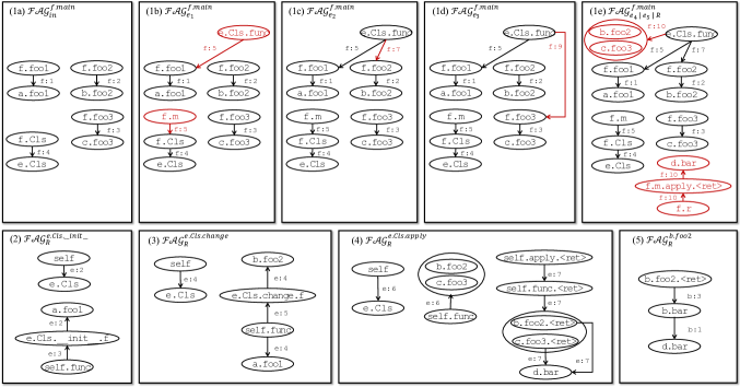
Figure 8. Function Assignment Graph for Jarvis

First, for each of $e$’s parent expressions (denoted as $e.p$), if the out-degree of $e.p$ in $\mathcal{CFG}_{f}$ is larger than 1 (Line 12), it means that the control flow diverges with $e$ as the first expression on the diverged flow. To enable flow-sensitive analysis, it creates a copy of $\mathcal{FAG}^{f}_{e.p}$, i.e., the FAG after $e.p$ is evaluated, for further update (Line 13).

Second, if $e$ has one parent in $\mathcal{CFG}_{f}$, the resulting points-to relations $\Delta_{e}$ from evaluating $e$ is updated to $\mathcal{FAG}^{f}_{e.p}$ for producing $\mathcal{FAG}^{f}_{e}$ (Line 15–18). The evaluation applies a transfer function, which is comprised of a list of transfer rules with respect to different expressions. Part of the transfer rules are reported in Fig. 7, and a full list is available at our website. Each transfer rule generates new points-to relations $\Delta_{e}$. Notice that if $e$ is a call expression, it runs inter-procedural analysis to compute $\Delta_{e}$ (see. Sec. 3.4.3). After $\Delta_{e}$ is computed, $\mathcal{FAG}^{f}_{e}$ is computed by adding $\Delta_{e}$ to $\mathcal{FAG}^{f}_{e.p}$.

Third, if $e$ has more than one parent, for all of $e$’s parent expressions, it merges their $\mathcal{FAG}^{f}_{e.p}$ into a new FAG $g_{merge}$ (Line 20), representing that the control flow converges. Then, it evaluates $e$ and adds newly generated points-to relations $\Delta_{e}$ to $g_{merge}$ (Line 21–22).

After all iterations finish, for each of the return expressions, i.e., $e\in\mathcal{CFG}_{f}.E_{r}$, there exists $\mathcal{FAG}^{f}_{e}$. Our analysis proceeds to over-approximately merge them into $\mathcal{FAG}^{f}_{R}$, i.e., the final FAG after all expressions in $f$ has been evaluated (Line 25).

Example 3.2.

Fig. 8(1a) shows the $\mathcal{FAG}^{f.main}_{in}$ before the function f.main in f.py in Fig. 2 is evaluated. As f.main does not have any parameter, $\mathcal{FAG}^{f.main}_{in}$ only contains points-to relations resulted from import expressions. For the ease of presentation, we use line number to denote the evaluated expression in points-to relations; e.g., f:1 denotes the import expression at the first line of f.py.

After $e_{1}$ (f:5) in the control flow graph in Fig. 5 is evaluated, two new points-to relations are produced (as highlighted by the red part in Fig. 8(1b)), and added to $\mathcal{FAG}^{f.main}_{in}$ to produce $\mathcal{FAG}^{f.main}_{e_{1}}$.

When our analysis proceeds to $e_{2}$ (f:7), the control flow diverges. Hence, our analysis creates a copy of $\mathcal{FAG}^{f.main}_{e_{1}}$, and adds the newly-created points-to relation e.Cls.func $\xrightarrow{f:7}$ f.foo2 to it for producing $\mathcal{FAG}^{f.main}_{e_{2}}$ (as shown in Fig. 8(1c)). Similarly, when $e_{3}$ (f:9) is evaluated, it first creates a copy of $\mathcal{FAG}^{f.main}_{e_{1}}$, and then adds the newly-created points-to relation e.Cls.func$\xrightarrow{f:9}$ f.foo3 for generating $\mathcal{FAG}^{f.main}_{e_{3}}$ (as shown in Fig. 8(1d)).

Next, when $e_{4}$ (f:10) is evaluated, the control flow converges. Thus, our analysis merges $\mathcal{FAG}^{f.main}_{e_{2}}$ and $\mathcal{FAG}^{f.main}_{e_{3}}$ by adding points-to relations that are only contained in $\mathcal{FAG}^{f.main}_{e_{3}}$ to $\mathcal{FAG}^{f.main}_{e_{2}}$ and then applying simplification (Fahndrich and Aiken, 1996) to $\mathcal{FAG}^{f.main}_{e_{2}}$. The merged points-to relation is e.Cls.func $\xrightarrow{f:10}$ {b.foo2, c.foo3}, as shown in Fig. 8(1e). Notice that the collapsed functions (i.e., b.foo2 and c.foo3) are caused by simplification. Then, the resulting points-to relations from evaluating $e_{4}$ is added to produce $\mathcal{FAG}^{f.main}_{e_{4}}$.

Finally, the evaluation of $e_{5}$ does not produce any new points-to relation. Thus, $\mathcal{FAG}^{f.main}_{e_{5}}$ is the same to $\mathcal{FAG}^{f.main}_{e_{4}}$. As there is only one return statement, $\mathcal{FAG}^{f.main}_{R}$ is the same to $\mathcal{FAG}^{f.main}_{e_{5}}$.

3.3.4. Compute Output FAG

Given $\mathcal{FAG}^{f}_{in}$ and $\mathcal{FAG}^{f}_{R}$, this step computes $\mathcal{FAG}^{f}_{out}$ (Line 27). Different from $\mathcal{FAG}^{f}_{R}$ which records possible points-to relations across all control flows, $\mathcal{FAG}^{f}_{out}$ is a subset of $\mathcal{FAG}^{f}_{R}$ where points-to relations about temporary variables are discarded and the rest of points-to relations are still in effect after the call to $f$ is returned. In particular, for each points-to relation $d_{1}\xrightarrow{e}d_{2}$ $\in$ $\mathcal{FAG}^{f}_{in}$, it first obtains $d_{1}$ from $\mathcal{FAG}^{f}_{in}$, and then computes definitions that $d_{1}$ finally points to in $\mathcal{FAG}^{f}_{R}$. Notice that it also computes definitions that the fields of $d_{1}$ finally point to. Concerning that $d_{1}$ may point to multiple definitions, it compares the order of evaluated expression for each points-to relation using $\mathcal{CFG}_{f}$ in order to select the latest result as $\mathcal{FAG}^{f}_{out}$.

Example 3.3.

In $\mathcal{FAG}^{f.main}_{R}$ in Fig. 8, there are three points-to relations from e.Cls.func, i.e., e.Cls.func $\xrightarrow{f:5}$f.foo1, e.Cls.func $\xrightarrow{f:7}$ f.foo2, and e.Cls.func $\xrightarrow{f:10}$ {b.foo2, c.foo3}. We can learn that the above three points-to relations are respectively resulted from evaluating $e_{1}$ (f:5), $e_{2}$ (f:7) and $e_{4}$ (f:10). According to $\mathcal{CFG}_{f}$, we can learn that $e_{4}$ is the successor of $e_{1}$ and $e_{2}$, and hence the points-to relation resulted from $e_{1}$ and $e_{2}$ are discarded.

3.4. Inter-Procedural Analysis

The algorithm of our inter-procedural analysis is shown in Alg. 2. It has three steps, i.e., Update CG, Compute $\theta_{call^{\prime}}$, and Compute $\Delta_{call^{\prime}}$.

Algorithm 2 Inter-Procedural Analysis

1${f}$, ${call^{\prime}}$, $\mathcal{FAG}^{f}_{call^{\prime}.p}$

2$\Delta_{call^{\prime}}$

3function inter_analysis

4     $f^{\prime}$ = updateCG$(call^{\prime},\mathcal{FAG}^{f}_{call^{\prime}.p},\mathcal{I},\mathcal{F},\mathcal{C})$

5     $\theta_{call^{\prime}}$ = compute$\theta_{call^{\prime}}$($\mathcal{FAG}^{f}_{call^{\prime}.p}$, $call^{\prime}$)

6     $\mathcal{FAG}^{f^{\prime}}_{in},\mathcal{FAG}^{f^{\prime}}_{out}$ = intra_analysis$(f^{\prime},\theta_{call^{\prime}})$

7     $\Delta_{call^{\prime}}$= compute$\Delta_{call^{\prime}}(\mathcal{FAG}^{f^{\prime}}_{in},\mathcal{FAG}^{f^{\prime}}_{out})$

8     return $\Delta_{call^{\prime}}$

9end function

3.4.1. Update CG

Jarvis generates call relations during our inter-procedural analysis (Line 2 in Alg. 2). Given inputs as the call expression $call^{\prime}$ at the caller function $f$ as well as the FAG after evaluating $call^{\prime}$’s parent expression $\mathcal{FAG}^{f}_{call^{\prime}.p}$, this step resolves the callee function $f^{\prime}$, and adds the call relation $\langle f,f^{\prime}\rangle$ to the call graph.

Specifically, $call^{\prime}$ can be in the form of a.b(...) or b(...). For the form of a.b(...), it first searches $\mathcal{FAG}^{f}_{call^{\prime}.p}$ for the class definitions that are pointed to by the invoking variable (e.g., a) of $call^{\prime}$. Then, for each searched class definition $d_{cls}$, it checks whether there exists a function definition $d_{b}$ whose name $d_{b}.n$ equals to the call name (e.g., b) of $call^{\prime}$ according to $\mathcal{C}.Incl$. If yes, the callee function $f^{\prime}$ is resolved; otherwise, it continues this procedure on the super class of $d_{cls}$ according to $\mathcal{C}.Hier$. In other words, the ancestor classes of $d_{cls}$ is searched along the inheritance hierarchy. If $f^{\prime}$ is still not resolved, it searches $\mathcal{FAG}^{f}_{call^{\prime}.p}$ for the module definition $d_{m}$ that is pointed to by the invoking variable (e.g., a) of $call^{\prime}$. Then, it searches $\mathcal{F}$ for the function definition $d_{b}$ that satisfies $d_{b}.n=\texttt{b}$ and $d_{b}.\phi=d_{m}.\phi.(d_{m}.n,\textbf{mod})$ (i.e., the function definition is imported through module import expression import...). If found, the callee function $f^{\prime}$ is resolved.

For the form of b(...), it obtains its call name (e.g., b). Then, it searches $\mathcal{F}$ for the function definition $d_{b}$ that satisfies $d_{b}.n=\texttt{b}$ and $d_{b}.\phi=f.\phi$ (i.e., the function definition is in the same module with $f$). If such a $d_{b}$ is found, the callee function $f^{\prime}$ is resolved; otherwise, it continues to search $\mathcal{I}$ for the points-to relation $\langle d_{s},d_{t},e\rangle$ that satisfies $d_{s}.n=\texttt{b}$ (i.e., the function definition is imported by function import expression from...import...). If found, $d_{t}$ is the callee function’s definition, and $f^{\prime}$ is resolved.

Example 3.4.

When evaluating $e_{4}$ in Fig. 5, our analysis creates a call relation $\langle\texttt{f.main},\texttt{e.Cls.apply}\rangle$ as f.m points to e.Cls and function e.Cls.apply is a function definition inside class e.Cls.

3.4.2. Compute $\theta_{call^{\prime}}$

This step selects relevant points-to relations $\theta_{call^{\prime}}$ from the caller’s FAG, and pass $\theta_{call^{\prime}}$ to the construction of the callee’s FAG (Line 3 in Alg. 2). In other words, $\theta_{call^{\prime}}$ is passed from the caller’s inter-procedural analysis into the callee’s intra-procedural analysis (Line 4). Specifically, $\theta_{call^{\prime}}$ contains points-to relations about invoking variable and argument variables of $call^{\prime}$, which can be directly selected from $\mathcal{FAG}^{f}_{call^{\prime}.p}$.

Example 3.5.

When $e_{1}$ in Fig. 5 is evaluated, our analysis prepares $\theta_{call^{\prime}}$ to jump into e.Cls.__init__ for the next intra-procedural analysis. As $e_{1}$ has one argument variable but no invoking variable, our analysis only selects one points-to relation f.foo1 $\xrightarrow{f:1}$ a.foo1 from $\mathcal{FAG}^{f.main}_{in}$ in Fig. 8(1a), and puts it to $\theta_{call^{\prime}}$. After $\theta_{call^{\prime}}$ is passed to our intra-procedural analysis on e.Cls.__init__ (see Sec. 3.3.1), the pointed function definition a.foo1 is pointed to by the corresponding parameter variable e.Cls.__init__.f, i.e., e.Cls.__init__.f $\xrightarrow{e:2}$a.foo1, as shown in Fig. 8(2).

3.4.3. Compute $\Delta_{call^{\prime}}$

$\Delta_{call^{\prime}}$ is computed as the result of our inter-procedural analysis, which is passed back to the previous intra-procedural analysis (Line 5 in Alg. 2). Given inputs as $\mathcal{FAG}^{f^{\prime}}_{in}$ which is the FAG before intra-procedural analysis and $\mathcal{FAG}^{f^{\prime}}_{out}$ which is the FAG after intra-procedural analysis, this step computes changed points-to relations from $\mathcal{FAG}^{f^{\prime}}_{in}$ to $\mathcal{FAG}^{f^{\prime}}_{out}$, and puts them into $\Delta_{call^{\prime}}$. In particular, for each points-to relation $d_{1}\xrightarrow{e_{1}}d_{2}$ in $\mathcal{FAG}^{f^{\prime}}_{out}$, if $d_{1}$ exists in a points-to relation $d_{1}\xrightarrow{e_{2}}d_{3}$ in $\mathcal{FAG}^{f^{\prime}}_{in}$, it searches $\mathcal{FAG}^{f^{\prime}}_{out}$ for the final pointed definition $d_{n}$ and adds a new points-to relation $d_{1}\xrightarrow{e_{3}}d_{n}$ to $\Delta_{call^{\prime}}$; and similarly, if a points-to relation about the field of $d_{1}$ exists in $\mathcal{FAG}^{f^{\prime}}_{out}$ but does not exist $\mathcal{FAG}^{f^{\prime}}_{in}$, this points-to relation is also added to $\Delta_{call^{\prime}}$.

Example 3.6.

Following Example 3.4, our analysis proceeds to conduct intra-procedural analysis on e.Cls.apply in Fig. 2(e). The $\theta_{call^{\prime}}$ for this intra-procedural analysis has two points-to relations, i.e., f.m $\xrightarrow{f:5}$ e.Cls and e.Cls.func $\xrightarrow{f:10}$ {b.foo2, c.foo3}; and our intra-procedural analysis initializes two points-to relations, i.e., self$\xrightarrow{e:6}$ e.Cls and self.func $\xrightarrow{e:6}$ {b.foo2, c.foo3}, as shown in Fig. 8(4). Using the two points-to relations, our analysis knows that the return of self.func points to the return of b.foo2 and c.foo3, therefore creating self.func.<ret> $\xrightarrow{e:7}$ {b.foo2.<ret>, c.foo3.<ret>}, as shown in Fig. 8(4). Recursively, our analysis jumps into b.foo2 and c.foo3. When jumping into b.foo2, it creates two points-to relations, i.e., b.foo2.<ret> $\xrightarrow{b:3}$ b.bar and b.bar $\xrightarrow{b:1}$ d.bar, as shown in Fig. 8(5). Then, $\Delta_{call^{\prime}}$ is computed as {b.foo2.<ret> $\xrightarrow{b:3}$ d.bar}, and passed back to the intra-procedural analysis on e.Cls.apply. Finally, in the inter-procedural analysis on e.Cls.apply, $\Delta_{call^{\prime}}$ is computed as {$\texttt{self.apply.<ret>}\xrightarrow{e:7}\texttt{d.bar}$}, and passed back to the intra-procedural analysis on f.main.

4. Evaluation

We have implemented Jarvis with more than 3.4k lines of Python code, and released the source code at our website https://pythonjarvis.github.io/ with all of our experimental data set.

4.1. Evaluation Setup

To evaluate the efficiency and effectiveness of Jarvis, we design our evaluation to answer two research questions.

• RQ1 Scalability Evaluation: What is Jarvis’s scalability compared with the state-of-the-art approach PyCG?

• RQ2 Accuracy Evaluation: What is Jarvis’s accuracy compared with the state-of-the-art approach PyCG?

Benchmarks. Following PyCG (Salis et al., 2021), we use two benchmarks, i.e., a micro-benchmark of 135 small Python programs, and a macro-benchmark of 6 real-world Python applications. In particular, we construct our micro-benchmark by extending the micro-benchmark used in PyCG, which contains 112 small Python programs covering a wide range of language features organized into 16 distinct categories. We extend it by respectively adding 4, 4, 5 and 5 programs into category arguments, assignments, direct calls and imports to have a more comprehensive coverage of the features. Besides, to make our micro-benchmark support evaluation on flow-sensitiveness, we create 5 programs into a new category control flow. The newly added programs are included in new categories superscripted with “$*$” (see Table. 3). For each benchmark program, we maintain the source code and the corresponding call graph described in JSON.

For our macro-benchmark, we use 6 Python applications that are selected under four criteria. For popularity, we query GitHub for popular Python projects which have over 1000 stars. For quality, we select projects which at least have development activities in the past one year, and we filter out demo projects, cookbooks, etc. For feasibility, to facilitate the manual call graph construction, we select real command-line projects which contains runnable test cases by reading the repository ReadMes and looking through the source code. For scalability evaluation, we conduct a dependency analysis to obtain the dependent libraries which are regarded as part of the whole program, and select projects whose whole program is not less than 100k LOC and 10k functions. Table. 1 reports the statistics about the selected Python applications, where LOC (A.) denotes the LOC in the application itself, LOC (W.) denotes the LOC in both application and its dependent libraries, Func. (W.) denotes the number of functions in both application and its dependent libraries, and Lib. denotes the number of dependent libraries.

Table 1. Statistics about Macro-Benchmark

Id.	Project	Stars	LOC (A.)	LOC (W.)	Func. (W.)	Lib.	Domain
P1	bpytop	9.0k	5.0k	120.5k	11.7k	201	*nix resource monitor
P2	sqlparse	3.1k	4.8k	108.4k	10.8k	191	SQL parser module
P3	TextRank-4ZH	2.8k	0.5k	515.3k	30.0k	237	text processing
P4	furl	2.4k	2.9k	109.3k	11.0k	190	url manipulation
P5	rich-cli	2.4k	1.1k	200.4k	18.6k	192	command line toolbox
P6	sshtunnel	1.0k	2.5k	141.4k	14.5k	202	remote SSH tunnels

RQ Setup. The experiments are conducted on a MacBook Air with Apple M1 Chip and 8GB memory. We compare scalability and accuracy of Jarvis with PyCG. As the result varies with regard to the scope of the analysis, we conduct experiments based on four scenarios, i.e., Exhaustive Application-Program call graph generation (E.A.), Exhaustive Whole-Program call graph generation (E.W.), Demand-Driven Application-Program call graph generation (D.A.), and Demand-Driven Whole-Program call graph generation (D.W.). The “demands” in D.A. and D.W. are a collections of application functions including those invoked from test cases and those have usages in the Python module which would be automatically executed as a main when the module is being executed or imported.

RQ1 is mainly evaluated on our macro-benchmark. We compare the time and memory performance of Jarvis and PyCG, which are measured using UNIX time and pmap command. We conduct this comparison only in E.A. and E.W. because PyCG does not support demand-driven call graph generation due to its intrinsic nature. Notice that PyCG also does not support whole-program call graph generation, and we adapt PyCG to support it (which in fact is straightforward). PyCG is analyzed in three configurations in E.A. and E.W., i.e., running one iteration (e.g., E.W. (1)), running two iterations (e.g., E.W. (2)), and waiting until it reaches a fixed-point (e.g., E.W. (m)). Besides, Jarvis is demand-driven, and we adapt it to support E.A. and E.W. by taking all the functions in the analysis scope as entry functions. Moreover, we measure the time and memory performance of Jarvis in D.A. and D.W. to observe its scalability.

RQ2 is evaluated on micro-benchmark and macro benchmark. For micro-benchmark, we compare Jarvis and PyCG with the number of programs whose generated call graph is complete and sound (C. for completeness and S. for soundness), and the correct, incorrect and missing call relations (TP, FP and FN) with respect to different feature categories. A call graph is complete when it does not contain any call relation that is FP, and is sound when it does not have any call relation that is FN. For macro-benchmark, we compare the precision and recall of Jarvis and PyCG in E.A., D.A. and D.W., but we do not compare them in E.W. because of the potentially huge effort in constructing the ground truth. Precision is calculated by the proportion of correctly generated call relations (i.e., $\mathcal{CG}_{Gen}.E$ $\cap$ $\mathcal{CG}_{GT}.E$) in the generated call relations (i.e., $\mathcal{CG}_{Gen}.E$), and recall is calculated by the proportion of correctly generated call relations in the ground truth (i.e., $\mathcal{CG}_{GT}.E$), as formulated in Eq. 1.

(1) $$Pre.=\frac{\mid\mathcal{CG}_{Gen}.E\cap\mathcal{CG}_{GT}.E\mid}{\mid\mathcal{CG}_{Gen}.E\mid}\mathrm{,~{}}Rec.=\frac{\mid\mathcal{CG}_{Gen}.E\cap\mathcal{CG}_{GT}.E\mid}{\mid\mathcal{CG}_{GT}.E\mid}$$

As PyCG does not support D.A. and D.W., we use PyCG to generate call graphs in E.A. and E.W., and prune the call graphs by only keeping the functions that are reachable from the entry functions.

Table 2. Scalability Results on Our Macro-Benchmark

Id.	PyCG										Jarvis
	E.A. (1)		E.A. (m)		E.W. (1)		E.W. (2)		E.W. (m)		E.A.		E.W.		D.A.		D.W.
T.	M.	T.	M.	T.	M.	T.	M.	T.	M.	T.	M.	T.	M.	T.	M.	T.	M.
P1	0.78	79	1.26	90	78.49	766	113.50	799	24h+	2.3G	1.22	61	48.43	1003	0.88	53	3.21	162
P2	0.55	36	1.01	40	48.83	702	76.29	855	24h+	5.7G	0.46	33	33.79	764	0.31	30	1.27	75
P3	0.16	24	0.19	24	1705.07	1630	1947.39	OOM	4h+	RE	0.19	24	1465.26	2061	0.18	24	6.57	314
P4	0.25	30	0.35	30	47.14	569	72.53	636	24h+	5.1G	0.30	32	34.35	775	0.22	29	0.86	57
P5	0.20	26	0.25	28	988.36	1431	2190.40	OOM	0.5h+	OOM	0.26	26	163.01	1523	0.21	25	7.82	381
P6	0.19	28	0.24	29	149.02	684	245.13	741	24h+	4.6G	0.25	26	62.69	1250	0.19	26	3.29	175
Avg.	0.36	37	0.55	40	502.82	963	774.21	757	16.7h+	4.4G+	0.45	33	301.26	1229	0.33	31	3.84	194

Ground Truth Construction. We reuse the ground truth for micro-benchmark from PyCG (Salis et al., 2021). For our newly-added programs in micro-benchmark, we build the ground truth manually, which is easy because they are simple programs.

For macro-benchmark, our construction is two-fold. On the one hand, we execute the test cases and collect call traces for each application using the embedded Python trace module (python -m trace –listfuncs $<$python_file$>$). The call traces span across the whole-program. Then, the call traces are transformed into the same format in micro-benchmark. The transformed call graph contains implicit call relations that are invisible and inherently invoked by the Python interpreter; e.g., with import keyword, Python interpreter invokes functions from _fronzen_importlib which is in fact not part of the whole program. We filter them out from the ground truth.

On the other hand, we enlarge the collection of call relations generated by test case execution by manually inspecting application functions (i.e., functions in application modules exclusive of library functions). Specifically, we go through the code of each application function, and add missing call relations. This step is to improve the imperfect construction result of call graph using test cases, i.e., the incomplete test cases might miss call relations. Three of the authors are involved in this procedure, which takes 4 person months.

In summary, we construct the ground truth of call graphs with a total number of 5,653 functions and 20,085 call relations.

4.2. Scalability Evaluation (RQ1)

The scalability results in terms of time and memory performance on our macro-benchmark are reported in Table. 2. Time (T.) is measured in seconds and memory (M.) is measured in MB if not specified.

In terms of time, both Jarvis and PyCG generate call graph in E.A. within a second. PyCG takes more time for more iterations in E.A. (i.e., from 0.36 seconds in E.A. (1) to 0.55 seconds in E.A. (m)). The gap becomes larger in E.W., where PyCG takes averagely 502.82 seconds in E.W. (1), and Jarvis takes averagely 301.26 seconds. As the iteration increases, PyCG crashes in two projects due to out-of-memory (OOM) and recursion error (RE). Specifically, PyCG runs out-of-memory in E.W. (2) and suffers recursion error in E.W. (m) on P3, while PyCG runs out-of-memory in E.W. (2) and E.W. (m) on P5. We record the consumed time immediately before PyCG is crashed. Thereby, the average time for PyCG in E.W. (2) and E.W. (m) is more than 774.21 seconds and more than 16.7 hours. Therefore, Jarvis runs 67% faster than PyCG in E.W. (1), and at least 157% faster than PyCG in E.W. (2). Furthermore, we also measure time for Jarvis’s demand-driven call graph generation. Jarvis takes 0.33 seconds for D.A. and 3.84 seconds for D.W., which significantly consumes less time than in exhaustive call graph generation.

In terms of memory, Jarvis consumes 4 MB less memory than PyCG in E.A. (1), and 7 MB less memory than PyCG in E.A. (m). When the analysis scope is expanded to whole program, PyCG consumes 266 MB less memory than Jarvis in E.W. (1). However, when the iteration number increases, PyCG consumes significantly more memory than Jarvis, and also suffers out-of-memory and recursion error in E.W. (2) and E.W. (m). Moreover, it takes Jarvis 31 MB in D.A. and 194 MB in D.W., which significantly consumes less memory than in exhaustive call graph generation.

4.3. Accuracy Evaluation (RQ2)

We present the accuracy results of Jarvis and PyCG on our micro-benchmark and macro-benchmark.

Micro-Benchmark. The accuracy results on our micro-benchmark are presented in Table. 3. In terms of completeness, PyCG generates call graphs that are complete for 107 programs. 23 of the incomplete cases come from our newly-added categories (superscripted with “$*$”) and the rest 5 incomplete cases come from the original category. Those incomplete cases generate call graphs with 30 false positives (FP). The majority (24) of the 30 false positives for PyCG locate in the five newly-added categories. Differently, Jarvis generates complete call graphs for 134 cases. Jarvis only generates one incomplete case with one false positive in decorators.

In terms of soundness, PyCG generates call graphs that are sound for 126 programs. The rest 9 unsound cases span in categories such as built-ins, control flow, assignment, dicts and lists. The unsound cases cause 18 false negatives. There are 7 false negatives in built-ins, ranking the top among other categories. In the meantime, Jarvis generates 113 sound call graphs. The unsound cases of Jarvis span in categories such as dicts, lists and built-ins. Jarvis generates 35 false negatives, while the majority (26) of the false negatives come from dicts and lists.

Macro-Benchmark. The accuracy results on our macro-benchmark are presented in Table. 4. In terms of precision, Jarvis achieves similar precision in E.A. and D.A. when compared with PyCG. Besides, PyCG achieves similar precision in E.A. (1) and E.A. (m), and in D.A. (1) and D.A. (m) due to the relatively small analysis scope. In D.W., PyCG’s precision drastically drops to 0.19, while Jarvis’s precision also greatly drops to 0.35, but is 84% higher than PyCG. The reason for the drop from E.A. to D.W. is two-fold. First, our ground truth can be incomplete especially for the call relations in dependent libraries. Second, there is a difference in measuring accuracy of call graph from exhaustive analysis to demand-driven analysis. To be more specific, in exhaustive analysis, accuracy is computed by comparing sets of call relations, whereas in demand-driven analysis, accuracy is computed by comparing chains of call relations from entry functions. Therefore, for demand-driven analysis, the impreciseness of call graph is magnified. In other words, if there exists one false positive call relation, the subsequent call relations along the generated call chain are all considered as false positives. The same reason also explains the precision drop from D.A. to D.W.; i.e., in demand-analysis, the larger the analysis scope, the longer the call chains, and the higher chance to introduce more false positives.

Moreover, we inspect the precision loss of PyCG against Jarvis. The major reason is that PyCG reports call relations disregarding control flows, whereas Jarvis is flow-sensitive. In addition, PyCG also reports false positives due to insufficient treatment of class inheritance. For example, for function calls invoked from base classes, it reports function calls in sub classes, but they actually do not exist in the sub classes. We also inspect the impreciseness of Jarvis. The major reason is correlated with false negatives whose reasons will be discussed in the next paragraphs. Jarvis conducts on-the-fly analysis assuming that it could retrieve complete points-to relations after evaluating each expression. If the points-to relations are not updated timely and Jarvis does not capture them because of unreachable function definitions, it would report false call relations because it uses the outdated points-to relations.

Table 3. Accuracy Results on Our Micro-Benchmark

Category	PyCG					Jarvis
C.	S.	TP	FP	FN	C.	S.	TP	FP	FN
arguments	6/6	6/6	14	0	0	6/6	6/6	14	0	0
assignments	4/4	3/4	13	0	2	4/4	3/4	13	0	2
built-ins	3/3	1/3	3	0	7	3/3	2/3	6	0	4
classes	22/22	21/22	65	0	1	22/22	22/22	66	0	0
decorators	6/7	7/7	22	1	0	6/7	6/7	21	1	1
dicts	12/12	11/12	21	0	2	12/12	0/12	6	0	17
direct calls	4/4	4/4	10	0	0	4/4	4/4	10	0	0
exceptions	3/3	3/3	3	0	0	3/3	3/3	3	0	0
functions	4/4	4/4	4	0	0	4/4	4/4	4	0	0
generators	6/6	6/6	18	0	0	6/6	4/6	16	0	2
imports	13/14	14/14	20	2	0	14/14	14/14	20	0	0
kwargs	2/3	3/3	9	1	0	3/3	3/3	9	0	0
lambdas	5/5	5/5	14	0	0	5/5	5/5	14	0	0
lists	7/8	7/8	15	1	2	8/8	3/8	8	0	9
mro	6/7	6/7	19	1	1	7/7	7/7	20	0	0
returns	4/4	4/4	12	0	0	4/4	4/4	12	0	0
arguments∗	0/4	4/4	8	4	0	4/4	4/4	8	0	0
assignments∗	0/4	4/4	4	4	0	4/4	4/4	4	0	0
direct calls∗	0/5	5/5	18	5	0	5/5	5/5	18	0	0
imports∗	0/5	5/5	7	4	0	5/5	5/5	7	0	0
control flow∗	0/5	3/5	17	7	3	5/5	5/5	20	0	0
Total	107/135	126/135	316	30	18	134/135	113/135	299	1	35

In terms of recall, Jarvis achieves a recall of 0.82 and 0.66 in E.A. and D.A., improving PyCG by 8% in both E.A. and D.A. In D.W. (1), Jarvis improves PyCG by 15%, while in D.W. (2), Jarvis improves PyCG by 10% on the four projects where PyCG does not crash. The recall of PyCG and Jarvis drops from E.A. to D.A., which is also mainly caused by the accuracy computing difference. In demand-driven analysis, if there exists one false negative call relation, the subsequent call relations along the call chain in the ground truth are all considered as false negatives. The same reason also explains the recall drop from D.A. to D.W.; i.e., in demand-driven analysis, the larger the analysis scope, the longer the call chains, and the higher chance to introduce more false negatives.

Furthermore, we inspect the recall gain of Jarvis against PyCG. The major reason is that Jarvis supports built-ins and control flow more comprehensively than PyCG. For example, regarding support for built-ins, PyCG misses the call builtins.split for the call expression ‘tel-num’.split(‘-’); and regarding control flow, PyCG does not handle the with statements, and thus ignores the relevant control flows. We also inspect the false negatives of Jarvis. The root causes for false negatives are two-fold. First, functions stored in list, tuple and dict are missing as our FAG does not maintain points-to relations for the above data structures. Second, functions invoked from dynamic linked libraries (e.g., math-python-*.so) are missing due to reflective invocations and Jarvis’s incapability of inter-procedural analysis of dynamic linked libraries.

Table 4. Accuracy Results on Our Macro-benchmark

Id.	PyCG												Jarvis
	E.A. (1)		D.A. (1)		E.A. (m)		D.A. (m)		D.W. (1)		D.W. (2)		E.A.		D.A.		D.W.
Pre.	Rec.	Pre.	Rec.	Pre.	Rec.	Pre.	Rec.	Pre.	Rec.	Pre.	Rec.	Pre.	Rec.	Pre.	Rec.	Pre.	Rec.
P1	0.99	0.84	1.00	0.83	0.99	0.84	1.00	0.83	0.20	0.60	0.20	0.61	0.99	0.92	1.00	0.93	0.31	0.66
P2	0.99	0.62	1.00	0.32	0.99	0.62	1.00	0.32	0.19	0.48	0.19	0.49	0.99	0.64	1.00	0.35	0.45	0.54
P3	1.00	0.87	1.00	0.90	1.00	0.87	1.00	0.90	0.20	0.28	-	-	1.00	0.95	1.00	0.90	0.37	0.36
P4	0.99	0.60	1.00	0.31	0.99	0.60	1.00	0.31	0.15	0.48	0.15	0.49	1.00	0.63	1.00	0.31	0.50	0.51
P5	0.96	0.82	1.00	0.78	0.96	0.82	1.00	0.78	0.14	0.51	-	-	1.00	0.95	1.00	0.94	0.17	0.64
P6	1.00	0.80	1.00	0.52	1.00	0.80	1.00	0.52	0.23	0.51	0.23	0.52	1.00	0.85	1.00	0.56	0.32	0.62
Aver.	0.99	0.76	1.00	0.61	0.99	0.76	1.00	0.61	0.19	0.48	0.19	0.53	0.99	0.82	1.00	0.66	0.35	0.55

4.4. Threats

The primary threats to the validity of our experiments is our benchmark and the construction of ground truth. For micro-benchmark, we add 23 programs that are written by two authors that have at least two years of Python programming experience in order to have a more complete coverage of language features. Although not meant to be exhaustive, we believe it is representative. Besides, the ground truth of these 23 programs is easy to build because they are all simple programs. For macro-benchmark, we carefully select 6 real-world Python applications. We believe they are representative because they are popular in community, well-maintained, feasible to run and large-scale in whole-program. However, the construction of their ground truth is a challenging task. Therefore, we construct it by two ways, i.e., automated test case execution, and manual investigation. The manual investigation is conducted by two of the authors independently, and another author is involved to resolve disagreement. We do not use the macro-benchmark (containing 5 projects) of PyCG as it only contains call relations in application code, and its ground truth is manually constructed. To the best of our knowledge, our macro-benchmark is the largest one.

5. Related Work

We review the literature related to points-to analysis, call graph generation and evaluation of call graph generation.

5.1. Points-to Analysis

Many research works have proposed to improve the precision of points-to analysis from different perspectives, e.g., combining call-site sensitivity with object sensitivity (Kastrinis and Smaragdakis, 2013; Lu et al., 2021a; Lhoták and Hendren, 2008), demand-driven points-to analysis (Späth et al., 2016), combining type-analysis with points-to analysis (Allen et al., 2015), selectively applying context-sensitive analysis w.r.t precision-critical methods (Li et al., 2018; Lu et al., 2021b). Hardekopf et al. (Hardekopf and Lin, 2007) propose to lazily collapse inclusion constraint cycles based on inclusion-based pointer analysis (Andersen, 1994) to reduce the scalability of online cycle detection. Wilson et al. (Wilson and Lam, 1995) summarize the effects of a procedure using partial transfer function (PTF), thus enabling context-sensitive analysis without reanalyzing at every call site. Johannes et al. (Späth et al., 2016) propose Boomerang, which is a demand-driven flow-sensitive and context-sensitive pointer analysis for Java. For increased precision and scalability, clients can query Boomerang with respect to particular calling contexts of interest. Our approach uses flow-sensitive points-to analysis by encoding point-to relations with flow information in function assignment graph and uses demand-driven analysis to skip the analysis of unreachable functions.

5.2. Call Graph Generation

Many call graph generation techniques are proposed for a variety of programming languages, e.g., Java (Vallée-Rai et al., 1999; IBM, 2017), Python (Salis et al., 2021), JavaScript (Nielsen et al., 2021), C/C++ (Milanova et al., 2004; Wilson and Lam, 1995; Andersen, 1994), Scala (Petrashko et al., 2016), etc.

In Java, to deal with the missing edges caused by their language features, many approaches are proposed to handle language features such as reflection (Sun et al., 2021; Sawin and Rountev, 2011; Bodden et al., 2011; Liu et al., 2017; Sui et al., 2017; Grech et al., 2017), foreign function interface (Lee et al., 2020), dynamic method invocation(Bodden, 2012), serialization (Santos et al., 2021), and library call (Zhang and Ryder, 2007). To deal with scalability issues, Ali et al. propose CGC (Ali and Lhoták, 2012) and Averroes (Ali and Lhoták, 2013) to approximate the call graph by considering application-only. CGC and Averroes generate application-only call graph by generating a quickly-constructed placeholder library that over-approximates the possible behavior of an original library, therefore avoiding the big cost on whole-program analysis. Such application-program analysis omits the inner calls from the library which may not be useful in some static analysis tasks (e.g., vulnerability propagation analysis). In face of demand-driven needs, some approaches consider only the influenced nodes compared to those exhaustive ones for the entire program (Agrawal et al., 2002; Heintze and Tardieu, 2001; Agrawal, 2000; Späth et al., 2016). Reif (Reif et al., 2016) proposes call graph generation for potential exploitable vulnerabilities and analysis for general software quality attributes dedicated to the practical needs of libraries.

In JavaScript, many approaches are proposed to handle language features such as reflection (Schäfer et al., 2013) and event-driven (Madsen et al., 2015). To deal with scalability issues, Feldthaus et al. (Feldthaus et al., 2013) approximate call graph by using field-based analysis, tracking method objects and ignoring dynamic property accesses which simplifies type analysis of variables, making the flow analysis lightweight. Madsen et al. (Madsen et al., 2013) combine pointer analysis with use analysis to save the effort on analyzing library API bodies. In Scala, Petrashko et al. (Petrashko et al., 2016) and Ali et al. (Ali et al., 2015) propose to handle polymorphism to enhance call graph generation.

In Python, Salis el al. (Salis et al., 2021) propose PyCG to generate practical call graph in Python that could efficiently and accurately generate call graph edges by handling several Python features, such as modules, generators, function closures, and multiple inheritance. PyCG outperforms Pyan (Fraser et al., 2019) and Depends (Zhang and Jin, 2018) in call graph generation. Besides, Hu et. al. (Hu et al., 2021) propose to link the missing edges caused by foreign function interfaces in Python. However, call graph generation for Python is still far from perfection. To overcome the drawbacks in Python call graph generation as summarized in Sec. 1, we propose a demand-driven call graph generation approach for Python whole-program, which is scalable and accurate.

5.3. Evaluating Call Graph Generation

Several studies have evaluated call graph generation tools for various languages such as C (Murphy et al., 1998), Java (Reif et al., 2018, 2019; Ali et al., 2019), and JavaScript (Antal et al., 2018). On the one hand, they provide guidance for users to choose and improve state-of-the-art call graph generation tools from their perspectives. In particular, Murphy has shed light on the design space for call graph generation tools based on the conclusion that software engineers have little sense of the dimensions of approximation in any particular call graph (Murphy et al., 1998). On the other hand, these studies report that there exist variances in the number, precision and type of call edges of call graph generation tools because of different treatments of language features. In Java ecosystem, Sui et al. (Sui et al., 2018) construct a micro-benchmark for dynamic language features to evaluate the soundness of Soot (Vallée-Rai et al., 1999), WALA (IBM, 2017) and Doop (Bravenboer and Smaragdakis, 2009). Besides, Sui et al. (Sui et al., 2020) also evaluate the soundness of Doop with real-world Java programs. Reif et al. (Reif et al., 2018, 2019) construct an extensive test suite covering language and API features in Java, and compare the soundness and time overhead of Soot, WALA, OPAL(Eichberg et al., 2018)  and Doop. Differently, Tip and Palsberg (Tip and Palsberg, 2000) explore the precision and scalability of different approaches for resolving virtual function calls (e.g., CHA (Dean et al., 1995), RTA (Bacon and Sweeney, 1996) and $k$-CFA (Allen, 1970; Shivers, 1991)). To the best of our knowledge, none of these studies address the scalability problem in Python language, and our work fills this gap.

6. Conclusions

In this paper, we have proposed a scalable demand-driven call graph generation approach Jarvis for Python. Jarvis is demand-driven, flow-sensitive, scalable to large programs and generates call graphs on-the-fly. Our evaluation has demonstrated that Jarvis is efficient and effective in both demand-driven and exhaustive whole-program call graph generation, and improves the state-of-the-art approach. In future, we plan to apply Jarvis to foster downstream applications in security analysis and debloating Python dependencies.

7. Data Availability

All the source code of Jarvis and data used in evaluation are available at our replication site https://pythonjarvis.github.io/.

References

- (1)
- Agrawal (2000) Gagan Agrawal. 2000. Demand-driven construction of call graphs. In Proceedings of the International Conference on Compiler Construction. 125–140.
- Agrawal et al. (2002) Gagan Agrawal, Jinqian Li, and Qi Su. 2002. Evaluating a demand driven technique for call graph construction. In Proceedings of the International Conference on Compiler Construction. 29–45.
- Ali et al. (2019) Karim Ali, Xiaoni Lai, Zhaoyi Luo, Ondřej Lhoták, Julian Dolby, and Frank Tip. 2019. A study of call graph construction for JVM-hosted languages. IEEE Transactions on Software Engineering 47, 12 (2019), 2644–2666.
- Ali and Lhoták (2012) Karim Ali and Ondřej Lhoták. 2012. Application-only call graph construction. In Proceedings of the 26th European Conference on Object-Oriented Programming. 688–712.
- Ali and Lhoták (2013) Karim Ali and Ondřej Lhoták. 2013. Averroes: Whole-program analysis without the whole program. In Proceedings of the 27th European Conference on Object-Oriented Programming. 378–400.
- Ali et al. (2015) Karim Ali, Marianna Rapoport, Ondřej Lhoták, Julian Dolby, and Frank Tip. 2015. Type-based call graph construction algorithms for Scala. ACM Transactions on Software Engineering and Methodology 25, 1 (2015), 1–43.
- Allen (1970) Frances E. Allen. 1970. Control Flow Analysis. In Proceedings of the Symposium on Compiler Optimization. 1–19.
- Allen et al. (2015) Nicholas Allen, Padmanabhan Krishnan, and Bernhard Scholz. 2015. Combining type-analysis with points-to analysis for analyzing Java library source-code. In Proceedings of the 4th ACM SIGPLAN International Workshop on State Of the Art in Program Analysis. 13–18.
- Andersen (1994) Lars Ole Andersen. 1994. Program analysis and specialization for the C programming language. Datalogisk Institut, Københavns Universitet.
- Antal et al. (2018) Gábor Antal, Péter Hegedus, Zoltán Tóth, Rudolf Ferenc, and Tibor Gyimóthy. 2018. Static javascript call graphs: A comparative study. In Proceedings of the IEEE 18th International Working Conference on Source Code Analysis and Manipulation. 177–186.
- Bacon and Sweeney (1996) David F Bacon and Peter F Sweeney. 1996. Fast static analysis of C++ virtual function calls. In Proceedings of the 11th ACM SIGPLAN conference on Object-oriented programming, systems, languages, and applications. 324–341.
- Barros et al. (2015) Paulo Barros, René Just, Suzanne Millstein, Paul Vines, Werner Dietl, Marcelo d’Amorim, and Michael D Ernst. 2015. Static analysis of implicit control flow: Resolving java reflection and android intents (t). In Proceedings of the 30th IEEE/ACM International Conference on Automated Software Engineering. 669–679.
- Bodden (2012) Eric Bodden. 2012. InvokeDynamic support in Soot. In Proceedings of the ACM SIGPLAN International Workshop on State of the Art in Java Program analysis. 51–55.
- Bodden et al. (2011) Eric Bodden, Andreas Sewe, Jan Sinschek, Hela Oueslati, and Mira Mezini. 2011. Taming reflection: Aiding static analysis in the presence of reflection and custom class loaders. In Proceedings of the 33rd International Conference on Software Engineering. 241–250.
- Bravenboer and Smaragdakis (2009) Martin Bravenboer and Yannis Smaragdakis. 2009. Strictly declarative specification of sophisticated points-to analyses. In Proceedings of the 24th ACM SIGPLAN conference on Object oriented programming systems languages and applications. 243–262.
- Bruce et al. (2020) Bobby R. Bruce, Tianyi Zhang, Jaspreet Arora, Guoqing Harry Xu, and Miryung Kim. 2020. JShrink: In-Depth Investigation into Debloating Modern Java Applications. In Proceedings of the 28th ACM Joint Meeting on European Software Engineering Conference and Symposium on the Foundations of Software Engineering. 135–146.
- Chess and McGraw (2004) Brian Chess and Gary McGraw. 2004. Static analysis for security. IEEE security & privacy 2, 6 (2004), 76–79.
- Dean et al. (1995) Jeffrey Dean, David Grove, and Craig Chambers. 1995. Optimization of object-oriented programs using static class hierarchy analysis. In Proceedings of the 9th European Conference on Object-Oriented Programming. 77–101.
- Eichberg et al. (2018) Michael Eichberg, Florian Kübler, Dominik Helm, Michael Reif, Guido Salvaneschi, and Mira Mezini. 2018. Lattice based modularization of static analyses. In Proceedings of the 7th International Workshop on the State Of the Art in Program Analysis. 113–118.
- Fahndrich and Aiken (1996) Manuel Fahndrich and Alex Aiken. 1996. Making Set-Constraint Program Analyses Scale. Technical Report.
- Feldthaus et al. (2013) Asger Feldthaus, Max Schäfer, Manu Sridharan, Julian Dolby, and Frank Tip. 2013. Efficient construction of approximate call graphs for JavaScript IDE services. In Proceedings of the 35th International Conference on Software Engineering. 752–761.
- Foundation (2023) Python Software Foundation. 2023. Abstract Syntax Tree - Python. Retrieved January 29, 2023 from https://docs.python.org/3/library/ast.html#expressions
- Fraser et al. (2019) David Fraser, Edmund Horner, Juha Jeronen, and Patrick Massot. 2019. Pyan3: Offline call graph generator for Python 3. Retrieved January 29, 2023 from https://github.com/davidfraser/pyan
- Grech et al. (2017) Neville Grech, George Fourtounis, Adrian Francalanza, and Yannis Smaragdakis. 2017. Heaps don’t lie: countering unsoundness with heap snapshots. Proceedings of the ACM on Programming Languages 1, OOPSLA (2017), 1–27.
- Guarnieri and Livshits (2009) Salvatore Guarnieri and V Benjamin Livshits. 2009. GATEKEEPER: Mostly Static Enforcement of Security and Reliability Policies for JavaScript Code. In Proceedings of the 18th conference on USENIX Security Symposium, Vol. 10. 78–85.
- Hardekopf and Lin (2007) Ben Hardekopf and Calvin Lin. 2007. The ant and the grasshopper: fast and accurate pointer analysis for millions of lines of code. In Proceedings of the 28th ACM SIGPLAN Conference on Programming Language Design and Implementation. 290–299.
- Heintze and Tardieu (2001) Nevin Heintze and Olivier Tardieu. 2001. Demand-driven pointer analysis. In Proceedings of the ACM SIGPLAN 2001 Conference on Programming Language Design and Implementation. 24–34.
- Hejderup et al. (2018) Joseph Hejderup, Arie van Deursen, and Georgios Gousios. 2018. Software ecosystem call graph for dependency management. In Proceedings of the IEEE/ACM 40th International Conference on Software Engineering: New Ideas and Emerging Technologies Results. 101–104.
- Hu et al. (2021) Mingzhe Hu, Yu Zhang, Wenchao Huang, and Yan Xiong. 2021. Static Type Inference for Foreign Functions of Python. In Proceedings of the IEEE 32nd International Symposium on Software Reliability Engineering. 423–433.
- Huang et al. (2022) Kaifeng Huang, Bihuan Chen, Congying Xu, Ying Wang, Bowen Shi, Xin Peng, Yijian Wu, and Yang Liu. 2022. Characterizing Usages, Updates and Risks of Third-Party Libraries in Java Projects. Empirical Software Engineering 27, 4 (2022), 1–41.
- IBM (2017) IBM. 2017. The T. J. Watson Libraries for Analysis (WALA).
- Jensen et al. (2009) Simon Holm Jensen, Anders Møller, and Peter Thiemann. 2009. Type analysis for JavaScript. In Proceedings of the 16th International Static Analysis Symposium. 238–255.
- Kastrinis and Smaragdakis (2013) George Kastrinis and Yannis Smaragdakis. 2013. Hybrid context-sensitivity for points-to analysis. In Proceedings of the 34th ACM SIGPLAN Conference on Programming Language Design and Implementation. 423–434.
- Lee et al. (2020) Sungho Lee, Hyogun Lee, and Sukyoung Ryu. 2020. Broadening horizons of multilingual static analysis: semantic summary extraction from C code for JNI program analysis. In Proceedings of the 35th IEEE/ACM International Conference on Automated Software Engineering. 127–137.
- Lhoták and Hendren (2008) Ondřej Lhoták and Laurie Hendren. 2008. Evaluating the benefits of context-sensitive points-to analysis using a BDD-based implementation. ACM Transactions on Software Engineering and Methodology 18, 1 (2008), 1–53.
- Li et al. (2018) Yue Li, Tian Tan, Anders Møller, and Yannis Smaragdakis. 2018. Precision-guided context sensitivity for pointer analysis. Proceedings of the ACM on Programming Languages 2, OOPSLA (2018), 1–29.
- Liu et al. (2017) Jie Liu, Yue Li, Tian Tan, and Jingling Xue. 2017. Reflection analysis for java: Uncovering more reflective targets precisely. In Proceedings of the IEEE 28th International Symposium on Software Reliability Engineering. 12–23.
- Livshits and Lam (2005) V Benjamin Livshits and Monica S Lam. 2005. Finding Security Vulnerabilities in Java Applications with Static Analysis. In Proceedings of the 14th Conference on USENIX Security Symposium. 271–286.
- Lu et al. (2021a) Jingbo Lu, Dongjie He, and Jingling Xue. 2021a. Eagle: CFL-reachability-based precision-preserving acceleration of object-sensitive pointer analysis with partial context sensitivity. ACM Transactions on Software Engineering and Methodology 30, 4 (2021), 1–46.
- Lu et al. (2021b) Jingbo Lu, Dongjie He, and Jingling Xue. 2021b. Selective Context-Sensitivity for k-CFA with CFL-Reachability. In Proceedings of the 28th International Static Analysis Symposium. 261–285.
- Madsen et al. (2013) Magnus Madsen, Benjamin Livshits, and Michael Fanning. 2013. Practical static analysis of JavaScript applications in the presence of frameworks and libraries. In Proceedings of the 9th Joint Meeting on Foundations of Software Engineering. 499–509.
- Madsen et al. (2015) Magnus Madsen, Frank Tip, and Ondřej Lhoták. 2015. Static analysis of event-driven Node.js JavaScript applications. In Proceedings of the 2015 ACM SIGPLAN International Conference on Object-Oriented Programming, Systems, Languages, and Applications. 505–519.
- Milanova et al. (2004) Ana Milanova, Atanas Rountev, and Barbara G Ryder. 2004. Precise call graphs for C programs with function pointers. Automated Software Engineering 11 (2004), 7–26.
- Murphy et al. (1998) Gail C Murphy, David Notkin, William G Griswold, and Erica S Lan. 1998. An empirical study of static call graph extractors. ACM Transactions on Software Engineering and Methodology 7, 2 (1998), 158–191.
- Nagy et al. (2021) Bence Nagy, Tibor Brunner, and Zoltán Porkoláb. 2021. Unambiguity of Python Language Elements for Static Analysis. In Proceedings of the IEEE 21st International Working Conference on Source Code Analysis and Manipulation. 70–75.
- Nielsen et al. (2021) Benjamin Barslev Nielsen, Martin Toldam Torp, and Anders Møller. 2021. Modular call graph construction for security scanning of Node. js applications. In Proceedings of the 30th ACM SIGSOFT International Symposium on Software Testing and Analysis. 29–41.
- Petrashko et al. (2016) Dmitry Petrashko, Vlad Ureche, Ondřej Lhoták, and Martin Odersky. 2016. Call graphs for languages with parametric polymorphism. In Proceedings of the 2016 ACM SIGPLAN International Conference on Object-Oriented Programming, Systems, Languages, and Applications. 394–409.
- Quach et al. (2018) Anh Quach, Aravind Prakash, and Lok Yan. 2018. Debloating Software through Piece-Wise Compilation and Loading. In Proceedings of the 27th USENIX Security Symposium. 869–886.
- Reif et al. (2016) Michael Reif, Michael Eichberg, Ben Hermann, Johannes Lerch, and Mira Mezini. 2016. Call graph construction for java libraries. In Proceedings of the 24th ACM SIGSOFT International Symposium on Foundations of Software Engineering. 474–486.
- Reif et al. (2019) Michael Reif, Florian Kübler, Michael Eichberg, Dominik Helm, and Mira Mezini. 2019. Judge: Identifying, understanding, and evaluating sources of unsoundness in call graphs. In Proceedings of the 28th ACM SIGSOFT International Symposium on Software Testing and Analysis. 251–261.
- Reif et al. (2018) Michael Reif, Florian Kübler, Michael Eichberg, and Mira Mezini. 2018. Systematic evaluation of the unsoundness of call graph construction algorithms for Java. In Proceedings of the 7th International Workshop on the State Of the Art in Program Analysis. 107–112.
- Salis et al. (2021) Vitalis Salis, Thodoris Sotiropoulos, Panos Louridas, Diomidis Spinellis, and Dimitris Mitropoulos. 2021. Pycg: Practical call graph generation in python. In Proceedings of the IEEE/ACM 43rd International Conference on Software Engineering. 1646–1657.
- Santos et al. (2021) Joanna CS Santos, Reese A Jones, Chinomso Ashiogwu, and Mehdi Mirakhorli. 2021. Serialization-aware call graph construction. In Proceedings of the 10th ACM SIGPLAN International Workshop on the State Of the Art in Program Analysis. 37–42.
- Santos et al. (2022) Joanna CS Santos, Reese A Jones, Chinomso Ashiogwu, and Mehdi Mirakhorli. 2022. Insight Exploring Cross-Ecosystem Vulnerability Impacts. In Proceedings of the Automated Software Engineering. 37–42.
- Sawin and Rountev (2011) Jason Sawin and Atanas Rountev. 2011. Assumption hierarchy for a CHA call graph construction algorithm. In Proceedings of the IEEE 11th International Working Conference on Source Code Analysis and Manipulation. 35–44.
- Schäfer et al. (2013) Max Schäfer, Manu Sridharan, Julian Dolby, and Frank Tip. 2013. Dynamic determinacy analysis. In Proceedings of the 34th ACM SIGPLAN Conference on Programming Language Design and Implementation. 165–174.
- Shivers (1991) Olin Grigsby Shivers. 1991. Control-flow analysis of higher-order languages or taming lambda. Carnegie Mellon University.
- Späth et al. (2016) Johannes Späth, Lisa Nguyen Quang Do, Karim Ali, and Eric Bodden. 2016. Boomerang: Demand-driven flow-and context-sensitive pointer analysis for java. In Proceedings of the 30th European Conference on Object-Oriented Programming. 1–26.
- Sui et al. (2018) Li Sui, Jens Dietrich, Michael Emery, Shawn Rasheed, and Amjed Tahir. 2018. On the soundness of call graph construction in the presence of dynamic language features-a benchmark and tool evaluation. In Proceedings of the Asian Symposium on Programming Languages and Systems. 69–88.
- Sui et al. (2017) Li Sui, Jens Dietrich, and Amjed Tahir. 2017. On the use of mined stack traces to improve the soundness of statically constructed call graphs. In Proceedings of the 24th Asia-Pacific Software Engineering Conference. 672–676.
- Sui et al. (2020) Li Sui, Jens Dietrich, Amjed Tahir, and George Fourtounis. 2020. On the recall of static call graph construction in practice. In Proceedings of the IEEE/ACM 42nd International Conference on Software Engineering. 1049–1060.
- Sun et al. (2021) Xiaoyu Sun, Li Li, Tegawendé F Bissyandé, Jacques Klein, Damien Octeau, and John Grundy. 2021. Taming reflection: An essential step toward whole-program analysis of android apps. ACM Transactions on Software Engineering and Methodology 30, 3 (2021), 1–36.
- TIOBE (2023) TIOBE. 2023. TIOBE Index for January 2023. Retrieved January 29, 2023 from https://www.tiobe.com/tiobe-index/
- Tip and Palsberg (2000) Frank Tip and Jens Palsberg. 2000. Scalable propagation-based call graph construction algorithms. In Proceedings of the 15th ACM SIGPLAN conference on Object-oriented programming, systems, languages, and applications. 281–293.
- Vallée-Rai et al. (1999) Raja Vallée-Rai, Phong Co, Etienne Gagnon, Laurie Hendren, Patrick Lam, and Vijay Sundaresan. 1999. Soot - a Java Bytecode Optimization Framework. In Proceedings of the 1999 Conference of the Centre for Advanced Studies on Collaborative Research.
- Wilson and Lam (1995) Robert P Wilson and Monica S Lam. 1995. Efficient context-sensitive pointer analysis for C programs. In Proceedings of the ACM SIGPLAN 1995 Conference on Programming Language Design and Implementation. 1–12.
- Zhang and Jin (2018) Gang Zhang and Wuxia Jin. 2018. Depends is a fast, comprehensive code dependency analysis tool. Retrieved January 29, 2023 from https://github.com/multilang-depends/depends
- Zhang and Ryder (2007) Weilei Zhang and Barbara G Ryder. 2007. Automatic construction of accurate application call graph with library call abstraction for Java. Journal of Software Maintenance and Evolution: Research and Practice 19, 4 (2007), 231–252.