Does Principal Component Analysis Preserve the Sparsity in Sparse Weak Factor Models?

Abstract

This paper studies the principal component (PC) method-based estimation of weak factor models with sparse loadings. We uncover an intrinsic near-sparsity preservation property for the PC estimators of loadings, which comes from the approximately upper triangular (block) structure of the rotation matrix. It implies an asymmetric relationship among factors: the rotated loadings for a stronger factor can be contaminated by those from a weaker one, but the loadings for a weaker factor is almost free of the impact of those from a stronger one. More importantly, the finding implies that there is no need to use complicated penalties to sparsify the loading estimators. Instead, we adopt a simple screening method to recover the sparsity and construct estimators for various factor strengths. In addition, for sparse weak factor models, we provide a singular value thresholding-based approach to determine the number of factors and establish uniform convergence rates for PC estimators, which complement Bai and Ng (2023). The accuracy and efficiency of the proposed estimators are investigated via Monte Carlo simulations. The application to the FRED-QD dataset reveals the underlying factor strengths and loading sparsity as well as their dynamic features.

JEL Classification: C12, C53, C55

Key Words: Factor number, Factor strength, Principal component, Rotation matrix, Sparse factor loadings, Sparsity preservation, Weak factors

1 Introduction

Factor models have been widely used in economics and finance. Until very recently, a large body of literature on factor models has built on the assumption that all factors are strong or pervasive in the sense that each factor can influence almost all cross-sectional units. Under this assumption, Bai and Ng (2002) and Bai (2003) establish the asymptotics of principal component (PC) estimators with $N$ units observed with $T$ periods. It is well known that the space spanned by the factors can be estimated consistently by the PC method with rate $\min\left(N^{1/2},T^{1/2}\right)$, and both the estimated factors and factor loadings are consistent up to some rotation matrices.

However, many empirical findings support the existence of weak factors with sparse factor loadings. For instance, both Stock and Watson (2002) and Ludvigson and Ng (2009) find that the extracted PC factors from a large set of standardized macroeconomic variables can only fit a few variables’ time series observations well, suggesting a sparsity structure in factor loadings. More recently, Kristensen (2017), Freyaldenhoven (2022a), and Uematsu and Yamagata (2023a, b) revisit the same dataset in Stock and Waston (2002) and further confirm the findings on loadings. In addition, Uematsu and Yamagata (2023a) find sparse factor loadings in the FRED-MD dataset (McCracken and Ng, 2016) and in firm security excess returns of the S&P 500 index. Another motivation for sparse factor loadings comes from the literature on hierarchical or group factor models, where the local factors have nonzero factor loadings only for some specific cross-sectional groups. For example, shocks due to oil supply may only affect industrial production sectors, but not the industry of service. In empirical asset pricing, it is expected that portfolios formulated by size or value factor are influenced by such factors, but portfolios formulated by the momentum factor may not be. For more examples of local/group factors, see Ando and Bai (2017) and Choi et al. (2021).

Due to the aforementioned reasons, weak factor models have gained immense popularity and attracted the attention of many researchers. For instance, Onatski (2012) shows that the PC estimate is inconsistent when the true factor loadings $\Lambda^{0}$ are weak enough such that $\Lambda^{0\prime}\Lambda^{0}$ has a positive definite (p.d.) limit as $N$ approaches infinity. More recently, Uematsu and Yamagata (2023a, b) propose a sparse orthogonal factor regression (SOFAR) estimator that uses $\ell_{1}$ regularization to achieve sparsity, and also provide a new inferential procedure to determine whether each component of the factor loadings is zero or not and prove that it controls false discovery rate (FDR) under a pre-assigned level; Freyaldenhoven (2022a) proposes a new class of estimators to determine the number of relevant factors in the presence of local factors, and Guo et al. (2022) investigate information criteria with a new penalty to determine the number of factors, which can be adaptive to the degree of factor pervasiveness and favor more parsimonious models; Bai and Ng (2023) investigate the large sample properties of static PC estimators for approximate factor models with general weak factor loadings and show that the PC estimators are still consistent and asymptotically normal; for factor-based forecasting with large sets of variables, Chao et al. (2022), Chao and Swanson (2022), and Giglio et al. (2022b) use pre-screening methods to select valid predictors when factor pervasiveness does not hold.

In this paper, we delve into the study of weak factor models with sparse factor loadings. A factor is called “sparsely weak” when it only affects a small subset of cross-sectional units. This is the same as the “sparsity-induced” weak factor in Uematsu and Yamagata (2023a, b). Instead of taking SOFAR of Uematsu and Yamagata (2023a), we follow Bai and Ng (2023) to consider the PC estimation since it is much simpler and free of tuning parameters. To recover the sparsity in factor loadings, we adopt a simple screening on the PC estimator of factor loadings. Our computation burden is almost negligible compared to the procedures with regularization in Uematsu and Yamagata (2023a, b).

Under the sparsity assumption on factor loadings, we show that PC estimators of factors, factor loadings, and the common components are still consistent, and further establish their asymptotic distributions and uniform convergence rates. In addition to the usual large sample properties of PC estimators, we find that the rotation matrix in PC estimation has a special structure that leads to nearly sparse PC estimates for factor loadings. Based on this finding, we further sparsify the loading estimator exactly by screening the estimated PC loadings. Then with the sparsified loading estimator, we can straightforwardly estimate distinct factor strengths consistently. Finally, we propose using singular value thresholding (SVT) to determine the number of factors in sparse weak factor models.

In summary, this paper studies the properties of PC estimates for weak factor models with sparse loadings and proposes a PC-based screening method to sparsify the estimator for factor loadings. It has the following additional contributions to the existing literature on weak factor models. First, under our sparsity assumption on factor loadings with mixed sparsity degrees, we establish the large sample properties of PC estimates for factors, factor loadings, and common components, respectively. In particular, we provide the uniform convergence rates for PC estimates, which complement Bai and Ng (2023). Second, we show that the PC estimators for loadings are still sparse, meaning the sparsity structure in factor loadings is nearly invariant to the rotation matrix induced by the PC method. To the best of our knowledge, our paper is the first to reveal this intrinsic sparsity preservation feature of the PC estimator. This result is also in sharp contrast to the common sense that the sparsity of factor loadings cannot be reserved due to the matrix rotation in PC estimation; see Bailey et al. (2021, BKP hereafter) and Freyaldenhoven (2022b). We show that the invariance of sparsity to rotation comes from the particular structure of the rotation matrix $Q$, which is an (approximately) upper triangular matrix. Third, given the invariance of sparsity of factor loadings to PC rotation, we can easily recover the sparsity of factor loadings by applying proper screening to the PC estimates of factor loadings. In some scenarios, it is important and necessary to recover the sparsity structure of factor loadings when the estimated factor loadings are used as “generated regressors”. For example, ignoring the sparsity structure of factor loadings will lead to an inconsistent estimator of risk premia in the empirical asset pricing model of Giglio and Xiu (2021) and Giglio et al. (2022a). Fourth, based on the sparse loading estimators, we provide straightforward estimators for all factor strengths and establish their consistency. This result improves BKP (2021) where only the strength of the strongest factor is identified and estimated. Lastly, we make a contribution to the determination of the number of factors in weak factor models. Research on selecting the number of factors in weak factor models is still very limited. We investigate the SVT approach and establish its consistency in determining the factor number.

It is worth mentioning that our work is also related to the large literature on sparsity pursuit in factor models. The sparse principal component analysis (SPCA) pursues a sparse structure in the estimation of factor loadings to achieve a good interpretation for extracted PC factors. In order to obtain PCs with sparse factor loadings, different penalties or threshold techniques to the fitted loadings are usually adopted. For example, Rapach and Zhou (2021) estimate sparse PCs for 120 monthly macroeconomic variables from the FRED-MD database by combining the $\ell_{1}$-norm restriction in factor loadings with the PC objective function; Pelger and Xiong (2022) construct sparse proximate factors by using the largest, say, $m$ eigenvalues, and show a weaker form of correlation consistency. They do not focus on whether the factor model being weak or not but investigate its sparse approximation, while our approach can be cast as a generalized version of Pelger and Xiong (2022) in terms of selecting $m$ adaptively to factor strengths. Freyaldenhoven (2022b) explores possible rotations of estimated loadings to recover sparsity. Based on consistently estimated factor loadings $\widehat{\Lambda}$, Freyaldenhoven (2022b) suggests minimizing the $\ell_{0}$-norm of rotated loadings ($\widehat{\Lambda}R)$: $\min_{R}||\widehat{\Lambda}R||_{0}$, subject to the rotation matrix $R$ being nonsingular, and implements solving the problem with a more feasible $\ell_{1}$-norm. His basic idea is to search among different rotations of the estimated loadings to achieve sparsity. If the true factor loadings are indeed sparse, this approach may identify the sparsity pattern. For other rotation-based methods of nearly-sparse factor loadings, see Despois and Doz (2022).

We would also like to compare our paper with the recent one by Bai and Ng (2023). Both of the two papers show the asymptotic properties of factors, loadings and common components in weak factor models with possibly heterogeneous factor strengths. In fact, to derive these theoretical results we are inspired by the novel proof in Bai and Ng (2023), e.g., by making use of several asymptotically equivalent rotation matrices. In spite of the overlapped targets, there are certain fundamental differences. The setup of Bai and Ng (2023) is more general allowing that the entries of $\Lambda^{0}$ are non-zero but small, whereas ours only admits sparsity induced weak factor models. Besides, our requirement of the minimal factor strength for estimation consistency, while still reasonable, is more stringent than Bai and Ng’s. We impose the stronger conditions in order to show that the rotation matrix is upper triangular. The upper triangularity reveals the sparsity preservation properties by PC estimators, which is our ultimate interest and yet not pursued by Bai and Ng (2023). Moreover, convergence rates of PC estimators may also be improved due to the upper triangularity. We also establish uniform convergence rates of these estimators, propose additional estimators for factor strengths and number of factors and prove their consistency in our setup. These questions are not formally addressed in Bai and Ng (2023), and yet may be of independent interest.

The rest of this paper is organized as follows. We formally introduce weak factor models with sparse factor loadings and the PC estimation in Section 2. In Section 3, we study the asymptotics of PC estimators for factors, factor loadings and the common components under the weak factor scheme, including consistency, asymptotic distributions, and uniform convergence rates. Based on the finding on the rotation matrix in Section 3, we propose a screening method to sparsify the estimated factor loadings and provide consistent estimators for factor strengths in Section 4. Section 5 discusses the determination of the number of factors for weak factor models. The Monte Carlo simulation and empirical application are reported in Section 6 and 7, respectively. Section 8 concludes. All technical proofs are relegated in the Appendix.

NOTATIONS. For a set $A$, let $|A|$ be its cardinality. Let $a\vee b=\max\left\{a,b\right\}$ and $a\wedge b=\min\left\{a,b\right\}$ for two real numbers $a$ and $b$. For two sequences $\left\{a_{n}\right\}$ and $\left\{b_{n}\right\}$, $a_{n}\lesssim b_{n}$ denotes $a_{n}/b_{n}$ is bounded and $a_{n}\asymp b_{n}$ denotes that both $a_{n}/b_{n}$ and $b_{n}/a_{n}$ are bounded. For two random sequences $\left\{a_{n}\right\}$ and $\left\{b_{n}\right\},$ $a_{n}\lesssim_{p}b_{n}$ denotes $a_{n}/b_{n}\$is stochastically bounded and $a_{n}\asymp_{p}b_{n}$ if $a_{n}\lesssim_{p}b_{n}$ and $b_{n}\lesssim_{p}a_{n}.$ For a square matrix $A$, $\mu_{\min}\left(A\right)$ and $\mu_{\max}\left(A\right)$ are the smallest and largest eigenvalue of $A$, respectively. For a matrix $B,$ let $\left\|B\right\|=\left[\text{Tr}\left(BB^{\prime}\right)\right]^{1/2}$ be its Frobenius norm and $\left\|B\right\|_{sp}=\mu_{\max}^{1/2}\left(B^{\prime}B\right)$ be its spectral norm. For a $n\times 1$ vector $a$, its $\ell_{0}$-norm is $\left\|a\right\|_{0}=\sum_{j=1}^{n}\mathbf{1}\left(a_{j}\neq 0\right)$, where $\mathbf{1}\left(\cdot\right)$ is the usual indicator function. Throughout, we use the running indices $s$ and $t$ for the $T$ observations, indices $i$, $j$ for the $N$ cross-sectional units, and $k$ and $l$ for the $r$ factors.

2 The Weak Factor Models with Sparse Loadings

2.1 The model setup

To fix ideas, let us consider a static factor model with the following representation

$$X_{it}=\lambda_{i}^{\prime}F_{t}+e_{it},$$ (2.1)

$i=1,\ldots,N$, $t=1,\ldots,T,$ where $X_{it}$ is the observed data for the $i$th individual at time $t$, $F_{t}$ is a $r\times 1$ vector of latent factors, $\lambda_{i}$ is the corresponding $r\times 1$ vector of factor loadings, and $e_{it}$ is the idiosyncratic error with possible weak dependence across $i$ or/and over $t$. Or we may write the factor model in a matrix form as

$$X=\Lambda F^{\prime}+e,$$ (2.2)

where $X$ and $e$ are both $N\times T$ matrices with $X(i,t)=X_{it}$ and $e(i,t)=e_{it}$, respectively, $\Lambda=\left(\lambda_{1},\ldots,\lambda_{N}\right)^{\prime}$, and $F=\left(F_{1},\ldots,F_{T}\right)^{\prime}$. Also for later reference, denote the $k$th column of $\Lambda$ by $\Lambda_{\cdot,k}=\left(\Lambda_{1,k},\ldots,\Lambda_{N,k}\right)^{\prime}$ and the $k$th column of $F$ by $F_{\cdot,k}=\left(F_{1,k},\ldots,F_{T,k}\right)^{\prime}$, $k=1,\ldots,r$. Throughout the paper, we let $F_{t}^{0}$ be the $r\times 1$ vector of true factors and $\lambda_{i}^{0}$ be the true loadings, with $F^{0}$ and $\Lambda^{0}$ being the corresponding matrices.

In a standard factor model, it is typically assumed that all factors are strong in the sense that the $r\times r$ matrix $\Lambda^{0\prime}\Lambda^{0}/N$ is a full rank matrix for a sufficiently large $N$ and it has a positive definite (p.d.) limit. In contrast, we allow that there are both strong and weak factors. A factor is (sparsely) weak when it is not persuasive in the sense that the proportion of its non-zero factor loadings diminishes at a certain rate. The number (in magnitude) of individuals effectively affected by the $k$th factor $F_{\cdot,k}^{0}$ is of order $N^{\alpha_{k}},$ $\alpha_{k}\in\left[0,1\right]$, and the strength of this factor can be represented by the degree parameter $\alpha_{k}$ (BKP, 2021) such that

$$\Lambda_{\cdot,k}^{0\prime}\Lambda_{\cdot,k}^{0}\asymp N^{\alpha_{k}},\;k=1,\ldots,r.$$ (2.3)

Obviously, a strong factor has degree $\alpha_{k}=1$. As BKP (2021) point out, for a factor with an extremely weak signal with $\alpha_{k}\in(0,1/2)$, it is not identified without priori restrictions and not relevant in most financial and macroeconomic applications. Moreover, Freyaldenhoven (2022a) discusses the reasons why only factors affecting proportionally more than $\sqrt{N}$ of individuals are relevant in arbitrage pricing theory (APT) and aggregate fluctuations in macroeconomics. Hence we restrict the factor strength so that $\alpha_{k}\in[\underline{\alpha},1]$ for $k=1,\ldots,r$ with some $\underline{\alpha}>1/2$. It may be also worth mentioning that the strength degree $\alpha_{k}$ defined in (2.3) is $N$-dependent (we suppress $N$ here) and thus may vary with samples.

Our setup allows that some or even all of factors in $F^{0}$ are weak in terms of potential sparsity of $\Lambda^{0}$. In such a model with latent factors, a standard normalization which one might want to impose is $T^{-1}F^{0\prime}F^{0}=I_{r}$ as in Uematsu and Yamagata (2023a) and Freyaldenhoven (2022a). However, this identification restriction is no longer innocuous as it is not compatible with sparsity of $\Lambda^{0}$ in general. In other words, a weak factor model (with a particular sparsity structure of $\Lambda^{0}$) is not invariant to an arbitrary rotation transformation. This insight is also shared by Bai and Ng (2023, Section 5.2) in terms of an overidentification restriction on $F^{0}$, implying that the aforementioned methods would incur a problem when the restriction fails to hold in general, as verified in our Monte Carlo simulations. Since our proposed methods hinge on the particular structure of the underlying sparsity, we leave $T^{-1}F^{0\prime}F^{0}$ unspecified ex ante for coherence (except for its being p.d.). It is also worth mentioning that the major findings for the weak factor model in this paper can be readily applied to deal with a rank-deficient model, as a rank-deficient model is equivalent to a weak factor model up to a rotation transformation; see Giglio et al. (2022a).

2.2 PC estimation

To begin with, we assume that the true number of factors $r$ is known, and leave the determination of $r$ in Section 5. The estimation of factors and their loadings is via the method of PC in minimizing

$$\underset{\Lambda,F}{\min}\frac{1}{NT}\sum_{i=1}^{N}\sum_{t=1}^{T}\left(X_{it}-\lambda_{i}^{\prime}F_{t}\right)^{2},$$

subject to the usual identification restriction that $F^{\prime}F/T=I_{r}$ and $\Lambda^{\prime}\Lambda$ being diagonal. The estimated factors, denoted by $\widetilde{F}$, is $\sqrt{T}$ times the eigenvectors corresponding to the $r$ largest eigenvalues of the $T\times T$ matrix $\frac{X^{\prime}X}{NT}$ in decreasing order. Then $\widetilde{\Lambda}=X\widetilde{F}/T$, and $\widetilde{e}=X-\widetilde{\Lambda}\widetilde{F}^{\prime}$. Also, let $\widetilde{V}=\operatorname{diag}\left(\widetilde{V}_{1},\ldots,\widetilde{V}_{r}\right)$ be the $r\times r$ diagonal matrix consisting of the $r$ largest eigenvalues of $\frac{X^{\prime}X}{NT}$ in decreasing order. We also define the common component estimator $\widetilde{C}=\widetilde{\Lambda}\widetilde{F}^{\prime}$ as the estimator for $C^{0}=\Lambda^{0}F^{0\prime}.$

Without loss of generality, we assume that the degrees of factor strength are arranged such that $1\geq\alpha_{1}\geq\ldots\geq\alpha_{r}\geq\underline{\alpha}$. Given the possibility that two factors may have the same degree of strength, e.g., there may be two strong factors or two weak ones with an equal strength, we can distribute $\alpha_{j}$’s into $G$ groups so that

$$\alpha^{[1]} =\left\{\alpha_{1},\ldots,\alpha_{m_{1}}:\alpha_{1}=\cdots=\alpha_{m_{1}}\right\},$$

$$\text{ }\vdots$$

$$\alpha^{[G]} =\left\{\alpha_{m_{G-1}+1},\ldots,\alpha_{r}:\alpha_{m_{G-1}+1}=\cdots=\alpha_{r}\right\},$$

with $G\leq r$, and $G=r$ when every factor’s strength is unique. For ease of notation, let us also define the cardinality of $\alpha^{[g]}$ by $r_{g}\equiv\lvert\alpha^{[g]}\rvert,$ for $g=1,\ldots,G.$ Clearly, $r=\sum_{g=1}^{G}r_{g}$. In addition, let $\alpha_{[j]}$ be the same strength shared in group $g$, i.e., $\alpha_{[g]}=\alpha_{m_{g}}$ for $g=1,\ldots,G.$ It is obvious that $\alpha_{1}=\alpha_{[1]}.$

3 Large Sample Properties for PC Estimators

3.1 Main assumptions and a key result on the eigenvalue matrix

We first define a scale matrix $A$ as follows,

$$A=\operatorname{diag}\left(N^{\alpha_{1}},\ldots,N^{\alpha_{r}}\right),$$

which will be frequently used in this paper. To study the large sample properties of PC estimators, we make the following assumptions on the weak factor models.

Assumption 1. $E\|F_{t}^{0}\|^{4}<\infty$ for $t=1,...,T$ and $T^{-1}F^{0\prime}F^{0}\rightarrow_{p}\Sigma_{F}$ as $T\rightarrow\infty$ for some p.d. matrix $\Sigma_{F}$.

Assumption 2. For the factor loadings,

(i) $0<\underline{\lambda}\leq\left\|\lambda_{i}^{0}\right\|\leq\overline{\lambda}<\infty$ for all $i$’s and some constants $\underline{\lambda}$ and $\overline{\lambda}$;

(ii) For the $k$th factor, the number of non-zero factor loading is $n_{k}\equiv\left\|\Lambda_{\cdot,k}^{0}\right\|_{0}\asymp N^{\alpha_{k}}$ for $\alpha_{k}\in[\underline{\alpha},1]$ with $\underline{\alpha}>1/2,$ for $k=1,\ldots,r;$

(iii) $A^{-1/2}\Lambda^{0\prime}\Lambda^{0}A^{-1/2}\rightarrow\Sigma_{\Lambda}^{\ast}$ as $N\rightarrow\infty$ for some p.d. matrix $\Sigma_{\Lambda}^{\ast}$.

Assumption 3. There exists a positive constant $M\leq\infty$, such that for all $N$ and $T$,

(i) $E(e_{it})=0$ and $E(e_{it}^{2})<M$ for all $i$ and $t;$

(ii) $E(e_{s}^{\prime}e_{t}/N)=\gamma_{N}(s,t)$, $\left|\gamma_{N}(s,s)\right|\leq M$ for all $s$, and $T^{-1}\sum_{s=1}^{T}\sum_{t=1}^{T}\left|\gamma_{N}(s,t)\right|\leq M$;

(iii) $E(e_{it}e_{jt})=\tau_{ij,t}$ with $\left|\tau_{ij,t}\right|\leq\tau_{ij}$ for all $t$ with some $\tau_{ij}>0$. In addition, for $\forall\mathcal{S}\subset\{1,\ldots,N\}$, $\sum_{j=1}^{N}\tau_{ij}\mathbf{1}\left(j\in\mathcal{S}\right)\leq M$ and $\left|\mathcal{S}\right|^{-1/2}T^{-1/2}\sum_{j=1}^{N}\sum_{t=1}^{T}\left(e_{it}e_{jt}-\tau_{ij,t}\right)\mathbf{1}\left(j\in\mathcal{S}\right)=O_{p}\left(1\right);$

(iv) For every $(t,s)$, $E\left|N^{-1/2}\sum_{i=1}^{N}\left[e_{is}e_{it}-E(e_{is}e_{it})\right]\right|^{4}\leq M$;

(v) $\left(n_{k}T\right)^{-1/2}\sum_{i=1}^{N}\sum_{t=1}^{T}F_{t}^{0}\lambda_{ik}^{0}e_{it}=O_{p}(1)$ for $k=1,\ldots,r$;

(vi) Define $\gamma_{N,F}(s,t)=N^{-1}E(F_{t}^{0}e_{t}^{\prime}e_{s})$ and $\varpi(s)=\left(NT\right)^{-1/2}\sum_{i=1}^{N}\sum_{t=1}^{T}\left[F_{t}^{0}e_{it}e_{is}-E(F_{t}^{0}e_{it}e_{is})\right]$. $\max_{s}\sum_{t=1}^{T}\left\|\gamma_{N,F}(s,t)\right\|^{2}\leq M$ and $\max_{s}E\left\|\varpi(s)\right\|^{2}\leq M$;

(vii) $E\left(N^{-1}\sum_{i=1}^{N}\left\|T^{-1/2}\sum_{t=1}^{T}F_{t}^{0}e_{it}\right\|^{2}\right)\leq M$;

(viii) The eigenvalues of $\Sigma_{\Lambda}^{\ast}\Sigma_{F}$ are distinct.

Assumption 4. $\left\|e\right\|_{sp}^{2}=O_{p}\left(\max\left\{N,T\right\}\right).$

Assumptions 1-2 are standard in the literature on panel factor models. Assumption 1 imposes a moment condition on the true factors and requires the existence of a p.d. probability limit of $T^{-1}F^{0\prime}F^{0}$. Assumption 2 imposes a boundedness condition on the norm of factor loading vectors, and specifies the sparse structure in factor loadings. The deterministic factor loadings can be relaxed to be stochastic with some moment conditions. Assumption 3 provides some conditions on factors, factor loadings, and errors. 3(i)-(iii) impose moment conditions on errors and allow for weak cross-sectional/serial dependence as Bai (2003). Note that Assumption 3(iii) is weaker than Bai (2003) and thus generalizes the counterpart under a strong factor model. Assumption 3(vi) is used by Su and Wang (2017), and it is not redundant since we do not assume $F_{t}^{0}$ and $e_{s}$ are independent. Assumption 4 is also adopted by Bai and Ng (2002, 2023) and Moon and Weidner (2017). It surely holds for independently identically distributed (iid) data with uniformly bounded $4$th moments, and may also hold for weakly dependent data across $i$ and $t.$

We first present one of the key interesting results for weak factor models via PC: the eigenvalue matrix $\widetilde{V}$ preserves the magnitude of factor strength, as stated in Proposition 3.1 below.

Proposition 3.1

Under Assumptions 1-4, we have $\widetilde{V}_{k}\asymp_{p}N^{\alpha_{k}-1}$ for $k=1,\ldots,r.$

Remark 1. Unlike in a strong factor model, the diagonal elements of matrix $\widetilde{V}$ vanish at various rates determined by their corresponding factor strengths. It raises more challenges to our asymptotic theory later involving $\widetilde{V}^{-1}$ frequently, whereas in a strong factor model all these terms are $O_{p}(1)$.

3.2 Consistency and asymptotic distributions

In this subsection, we establish the consistency and asymptotic distributions for PC estimators. To reveal the asymptotic properties of our estimators, it is necessary to introduce several rotation matrices as below. We have suppressed the dependence on sample sizes for these matrices to ease burden of notations. Define

$$H = \frac{\Lambda^{0\prime}\Lambda^{0}}{N}\frac{F^{0\prime}\widetilde{F}}{T}\widetilde{V}^{-1},\text{ }H_{1}=\Lambda^{0\prime}\Lambda^{0}(\widetilde{\Lambda}^{\prime}\Lambda^{0})^{-1},\text{ }H_{2}=\left(F^{0\prime}F^{0}\right)^{-1}F^{0\prime}\widetilde{F},\text{ }$$

$$H_{3} = Q^{-1}\text{ with\ }Q=\frac{\widetilde{F}^{\prime}F^{0}}{T},\text{ and }H_{4}=\Lambda^{0\prime}\widetilde{\Lambda}(\widetilde{\Lambda}^{\prime}\widetilde{\Lambda})^{-1}.$$

We will show the asymptotic equivalence of the matrices $H$ and $H_{j}$ for $j=1,2,3,4,$ which also generalizes Lemma 3 of Bai and Ng (2023). These rotation matrices and the equivalence results will play an indispensable role in establishing the convergence rates and the asymptotic distributions of our PC estimators. Before doing so, we would like to first introduce an interesting finding related to the matrix $Q$ defined above. One more additional condition is needed.

Assumption 5. $N^{1-\alpha_{r}}/T^{1/2}\rightarrow 0$.

It is worth mentioning that Bai and Ng (2023) impose a weaker condition $N^{1-\alpha_{r}}/T$ $\rightarrow 0$ for consistency. They do not impose $N^{1-\alpha_{r}}/T^{1/2}\rightarrow 0$ until in proving distributional theory. However, we impose Assumption 5 at an early stage in this paper to obtain our main result stated in Proposition 3.2, which is fundamental in sparsity recovery results in Section 4. Besides, a sharper result may be obtained for consistency rate, e.g., Proposition 3.4, by making use of Proposition 3.2 valid under Assumption 5. Also note that under $N/T\rightarrow c\in\left(0,\infty\right)$ as assumed by Freyaldenhoven (2022a), Assumption 5 is trivial.

Proposition 3.2

Under Assumptions 1-5, the $r\times r$ matrix $Q=T^{-1}\widetilde{F}^{\prime}F^{0}$ is a full rank matrix in probability and

$$Q_{lk}\equiv Q\left(l,k\right)\asymp_{p}N^{\alpha_{l}-\alpha_{k}}\text{ for }1\leq k\leq l\leq r.$$

Remark 2. Proposition 3.2 implies a very important property of $Q$ serving as the rotation matrix: $Q$ is (block) upper triangular asymptotically. Such a property is very helpful in working with the sparsity-induced weak factor models.

Next, we state the convergence rate of $\widetilde{F}$ in the following proposition.

Proposition 3.3

Under Assumptions 1-5,

$$\frac{1}{T}\left\|\widetilde{F}-F^{0}H\right\|^{2}=O_{p}\left(N^{\alpha_{1}-2\alpha_{r}}+N^{2\left(1-\alpha_{r}\right)}T^{-2}\right)=o_{p}\left(1\right).$$

Remark 3. The associated convergence rate for Proposition 3.3 from Bai and Ng (2023, Proposition 6.i) is $O_{p}\left(N^{-\alpha_{r}}+N^{2\left(1-\alpha_{r}\right)}T^{-2}\right)=o_{p}\left(1\right)$, which is a bit better than ours. The reason is that they use a slightly different rotation matrix from ours $H$, as indicated by the comment below their Proposition 6. The reason behind our choice of the rotation matrix $H$ is that it is more closely related to $Q$ playing a major role in our later analysis.

The convergence rate for factor loading estimate is provided in the next proposition.

Proposition 3.4

Under Assumptions 1-5,

$$\frac{1}{N}\left\|\widetilde{\Lambda}-\Lambda^{0}Q^{\prime}\right\|^{2}=O_{p}\left(N^{-\alpha_{r}-1}+T^{-1}\right)=o_{p}\left(1\right).$$

Remark 4. Note that our rate in Proposition 3.4 is better than what is stated in Bai and Ng (2023, Proposition 6.ii). The reason is that we utilize the upper triangularity of rotation $Q$ in our proof, which helps sharpen the bound for estimation errors.

Before proceeding, we present here the equivalence results of $H$ and $H_{j}$ for $j=1,2,3,4.$ Define $\gamma_{NT}\equiv\max\left(N^{\frac{\alpha_{1}}{2}-\alpha_{r}}T^{-1/2},N^{1-\alpha_{r}}T^{-1},N^{-\alpha_{r}}\right).$

Lemma 3.5

Under Assumptions 1-5,

$$H_{j}=H+O_{p}\left(\gamma_{NT}\right),\text{ for }j=1,2,3,4.$$

Recall that $H_{3}=Q^{-1},$ and Lemma 3.5 thus implies that $Q^{-1}=H+O_{p}\left(\gamma_{NT}\right).$ This equivalence immediately implies the consistent estimation of the common component $\widetilde{C}.$ Lemma 3.5 generalizes Lemma 1 of Bai and Ng (2019) for strong factor models, and Lemma 3 of Bai and Ng (2023) for weak factor models with a single strength.

Proposition 3.6

Under Assumptions 1-5,

$$\frac{1}{NT}\left\|\widetilde{C}-C^{0}\right\|^{2}=O_{p}\left(N^{2\left(\alpha_{1}-\alpha_{r}\right)-1}+T^{-1}\right)=o_{p}\left(1\right).$$

Remark 5.  It is noted in Proposition 3.6 that the convergence rate of $\widetilde{C}$ in general depends on weak factor strengths, or precisely, the discrepancy of strengths between the strongest and weakest factors. It is only when all factor strengths are the same that the convergence rate is maximal and coincides with that under strong factor models. Also note that this result agrees with Bai and Ng (2023, Proposition 3) in considering homogeneous factor strength.

Now we turn to the asymptotic distributions of PC estimators. We impose the following assumption for establishing the central limit theorem (CLT), which is adaptive to weak factor models.

Assumption 6. The following hold for each $i$ and $t$ as $N,T\rightarrow\infty:$

(i) $A^{-1/2}\Lambda^{0\prime}e_{t}\overset{d}{\rightarrow}N\left(0,\Gamma_{t}\right),$ where $\Gamma_{t}=\lim_{N\rightarrow\infty}A^{-1/2}\sum_{i=1}^{N}\sum_{j=1}^{N}\lambda_{i}^{0}\lambda_{j}^{0\prime}E\left(e_{it}e_{jt}\right)A^{-1/2}.$

(ii) $T^{-1/2}\sum_{t=1}^{T}F_{t}^{0}e_{it}\overset{d}{\rightarrow}N\left(0,\Phi_{i}\right),$where $\Phi_{i}=\lim_{T\rightarrow\infty}T^{-1}\sum_{s=1}^{T}\sum_{t=1}^{T}E\left(F_{t}^{0}F_{s}^{0\prime}e_{it}e_{is}\right).$

One more regularity condition is imposed on sample size ($N,T$) and the weakest factor strength $\alpha_{r}$ to guarantee the distributional theory, which is also used by Bai and Ng (2023, Assumption C’(iv)).

Assumption 7. $N^{\frac{3}{2}-\alpha_{r}}T^{-1}\rightarrow 0$.

Theorem 3.7

Under Assumptions 1-7,

$$A^{1/2}\left(\widetilde{F}_{t}-H_{4}F_{t}^{0}\right)\overset{d}{\rightarrow}N\left(0,\Psi^{0}\Gamma_{t}\Psi^{0\prime}\right),$$

where $\Psi^{0}=\mathop{\mathrm{p}lim}_{N,T\rightarrow\infty}N^{-1}A^{1/2}\widetilde{V}^{-1}QA^{1/2}.$

Remark 6. (i) As shown in the proof of Theorem 3.7, the matrix$\ \Psi^{0}$ is (block) diagonal. In particular, if no two factors have the same strength, i.e., $\alpha_{k}\neq\alpha_{l}$ for $k\neq l,$ then $\Psi^{0}$ is an exactly diagonal matrix so that $\Psi^{0\prime}=\Psi^{0}.$ (ii) Theorem 3.7 also reveals that the $k$th factor $\widetilde{F}_{tk}$ is asymptotically normally distributed with convergence rate of $N^{\alpha_{k}/2}.$

Assumption 8. $\sqrt{T}N^{-\alpha_{r}}\rightarrow 0$.

Theorem 3.8

Under Assumptions 1-8,

$$\sqrt{T}\left(\widetilde{\lambda}_{i}-Q\lambda_{i}^{0}\right)\overset{d}{\rightarrow}N\left(0,Q^{\prime-1}\Phi_{i}Q^{-1}\right).$$

Remark 7. Theorem 3.8 reveals that the asymptotic distribution of $\widetilde{\lambda}_{i}$ is the same under both strong and weak factors and invariant to factor strengths.

With Theorems 3.7 and 3.8, we come to the limiting distribution of $\widetilde{C}_{it}.$ To this end, recall $r_{G}$ from Section 2.2, and define the $r\times r$ matrix $S^{\dagger}=\operatorname{diag}(\underbrace{0,\ldots,0}_{r-r_{G}},\underbrace{1\ldots,1}_{r_{G}})$.

Theorem 3.9

Under Assumptions 1-8,

$$\frac{\widetilde{C}_{it}-C_{it}^{0}}{\sqrt{N^{-\alpha_{r}}V_{it}+T^{-1}U_{it}}}\overset{d}{\rightarrow}N\left(0,1\right),$$

where $V_{it}=\lambda_{i}^{0\prime}S^{\dagger}\Sigma_{\Lambda}^{\ast-1}\Gamma_{t}\Sigma_{\Lambda}^{\ast-1}S^{\dagger}\lambda_{i}^{0}$ and $U_{it}=F_{t}^{0\prime}\Sigma_{F}^{-1}\Phi_{i}\Sigma_{F}^{-1}F_{t}^{0}.$

Remark 8. Theorem 3.9 thus implies that $\widetilde{C}_{it}-C_{it}^{0}=O_{p}\left(\max\left\{N^{-\alpha_{r}/2},T^{-1/2}\right\}\right).$ As for the asymptotic covariance matrix for $\widetilde{F}_{t}$ ($\widetilde{\lambda}_{i}),$ Bai and Ng (2023) have proposed consistent estimators assuming cross-section (serial) independence for $\left\{e_{it}\right\}.$ Under weakly serial dependence, Bai (2003) proposes a consistent Newey-West HAC estimator for the asymptotic covariance of $\widetilde{\lambda}_{i}.$ For estimating the asymptotic covariance of $\widetilde{F}_{t}$ under weakly cross-section (CS) independence, Bai and Ng (2006) propose a consistent CS-HAC estimator under covariance stationarity with $E\left(e_{it}e_{jt}\right)=\sigma_{ij}$ for all $t$’s. One could follow the aforementioned approaches to formulate consistent estimators of the asymptotic covariance matrices for $\widetilde{F}_{t}$ and $\widetilde{\lambda}_{i},$ which would lead to a consistent variance estimator for $\widetilde{C}_{it}$. For hypothesis testing, with $\widetilde{F}_{t}$ for instance, there is no need to know factor strengths, as the feasible estimator for the variance of $\widetilde{F}_{t}$ automatically accommodates factor strengths, and is thus adequate for such a purpose.

3.3 Uniform convergence rates

In this section, we will establish uniform convergence rate results for $\widetilde{F}_{t}$, $\widetilde{\lambda}_{i},$ and $\widetilde{C}_{it}$ over $i$ or (and) $t.$ These results can be exploited in recovering model sparsity in Section 4, in the potential application of factor-augmented forecast regression, and are perhaps also of independent interest.

Given that dependence is allowed across both $i$ and $t$, we first define a strong mixing condition, generalized over $i$ and $t,$ similar to Ma et al. (2021). Suppose that there is some labeling of the cross-sectional units $i_{l_{1}},\ldots,i_{l_{N}},$ whose generic index we denote by $i^{\ast},$ such that the CS dependence decays with distance $\left|i^{\ast}-j^{\ast}\right|.$ Then we will define a mixing rate applied for the random field $\left\{G_{i^{\ast}t}:1\leq i^{\ast}\leq N,1\leq t\leq T\right\},$ where $G_{i^{\ast}t}\equiv\left(F_{t}^{0\prime},e_{i^{\ast}t}\right)^{\prime}.$ For $S_{1},S_{2}\subset\left[1,\ldots,N\right]\times\left[1,\ldots,T\right],$ let

$$\alpha\left(S_{1},S_{2}\right)\equiv\sup\left\{\left|P\left(A\right)P\left(B\right)-P\left(A\cap B\right)\right|:A\in\sigma\left(G_{i^{\ast}t},\left(i^{\ast},t\right)\in S_{1}\right),B\in\sigma\left(G_{i^{\ast}t},\left(i^{\ast},t\right)\in S_{2}\right)\right\},$$

where $\sigma\left(\cdot\right)$ denotes a sigma-field. Then the $\alpha$-mixing coefficient of $\left\{G_{i^{\ast}t}\right\}$ is defined as

$$\alpha\left(k\right)\equiv\sup\left\{\alpha\left(S_{1},S_{2}\right):d\left(S_{1},S_{2}\right)\geq k\right\},$$

where $d\left(S_{1},S_{2}\right)\equiv\min\left\{\sqrt{\left(t-s\right)^{2}+\left(i^{\ast}-j^{\ast}\right)^{2}}:\left(i^{\ast},t\right)\in S_{1},\left(j^{\ast},s\right)\in S_{2}\right\}.$

The definition of $\alpha\left(k\right)$ generalizes the usual one in the time series context. In particular, when $\alpha\left(k\right)$ is applied to to a (single or vector of) time series, it coincides with the usual one defined by, e.g., Fan et al. (2011). (ii) For the purpose of estimation, we do not need to know the true labeling $\left\{i^{\ast}\right\}.$ Ma et al. (2021) show that their inference is valid as long as the number of mis-assigned indices is $o\left(N^{1/2}\right).$ In conducting inference, our approach is effective with the true labeling $\left\{i^{\ast}\right\}$ completely unknown, and thus further relaxes the assumption by Ma et al. (2021).

We now specify the additional assumptions for the uniform results.

Assumption 9. (i) $\left\{e_{t}\right\}_{t\geq 1}$ and $\left\{F_{t}^{0}\right\}_{t\geq 1}$ are both stationary and ergodic;

(ii) There exists $s_{2}>0$ and $K>0$ such that $\forall t\in\mathbb{Z}^{+},$ $\alpha\left(t\right)\leq\exp\left(-Kt^{s_{2}}\right);$

(iii) There exists $s_{1}>0,$ $b_{1}>0,$ $s_{3}>0,$ $b_{2}>0,$ satisfying $3s_{1}^{-1}+s_{2}^{-1}>1$ and $3s_{3}^{-1}+s_{2}^{-1}>1$, such that $\forall w>0,$ $P\left(\left|e_{it}\right|>w\right)\leq\exp\left(-\left(w/b_{1}\right)^{s_{1}}\right)$ and $P\left(\left|F_{tk}^{0}\right|>w\right)\leq\exp\left(-\left(w/b_{2}\right)^{s_{3}}\right)$ for $k=1,...,r;$

(iv) $\left(\ln N\right)^{2/\gamma_{2}-1}=o\left(T\right),$ where $\gamma_{2}=1.5s_{1}^{-1}+1.5s_{3}^{-1}+s_{2}^{-1}.$

From the previous section, we see that the PC estimators $\widetilde{F}_{t}$ and $\widetilde{\lambda}_{i}$ are both consistent up to a certain rotation matrix. So to better state the uniform convergence result, we define the rotated factor and factor loading by $\lambda_{i}^{\ast}\equiv Q\lambda_{i}^{0}$ and $F_{t}^{\ast}=H_{4}^{\prime}F_{t}^{0},$ respectively.

Theorem 3.10

Under Assumptions 1-9,

(i) $\sup_{i}\left|\widetilde{\lambda}_{ik}-\lambda_{ik}^{\ast}\right|=O_{p}\left(\sqrt{(\ln N)/T}\right)$ for $k=1,...,r;$

(ii) $\sup_{t}\left|\widetilde{F}_{tk}-F_{tk}^{\ast}\right|=O_{p}\left(N^{-\alpha_{k}/2}\sqrt{\ln T}\right)$ for $k=1,...,r;$

(iii) $\sup_{i,t}\left|C_{it}-C_{it}^{0}\right|=O_{p}\left(\left(\ln T\right)^{1/s_{3}}\sqrt{(\ln N)/T}+N^{-\alpha_{r}/2}\sqrt{\ln T}\right).$

Remark 9. In Theorem 3.10, result (i) implies that the estimation errors for factor loadings are uniformly dominated by $\sqrt{(\ln N)/T}$. This result is very useful to explore loading sparsity and factor strength in the next section. For each factor, result (ii) provides the uniform convergence rate which depends on the factor strength. Result (iii) establishes the uniform convergence rate for the common component estimators and the rate is determined by the smallest factor strength $\alpha_{r}$ and a parameter $s_{3}$ which controls the probability tail bound of factors.

4 Revelation of the Sparsity in Loadings with PC Estimators

It is well known that latent factor models are subject to a rotational indeterminacy. This identification issue is unwanted to reveal the loading sparsity structure. Specifically, our results in Section 2 indicates that loadings are identified only up to the rotation $Q$, and it is believed that a rotation in general plays a deterrent role in revealing sparsity. As a result, interpretation of estimated factors becomes intimidating, as it is usually drawn in a manner by relating to observables which an individual factor loads on primarily. For example, Ludvigson and Ng (2009) write,

“Moreover, we caution that any labeling of the factors is imperfect, because each is influenced to some degree by all the variables in our large dataset and the orthogonalization means that no one of them will correspond exactly to a precise economic concept like output or unemployment, which are naturally correlated.”

However, we show that even in the presence of the rotation $Q$ brought in by PC, the sparsity in factor loadings can still be preserved. This justifies the ad hoc manner of interpretation of PC factors with only a small set of variables or individuals in many empirical applications; see Pelger and Xiong (2022).

4.1 Preservation of sparsity degree by the PC rotation

The success of sparsity preservation by PC largely hinges on the property of the particular rotation matrix $Q$. Proposition 3.2 implies that $Q$ is a non-strictly (block) upper triangular matrix with full rank in probability. In particular,

$$Q_{lk}\begin{cases}\asymp_{p}N^{\alpha_{l}-\alpha_{k}},\;\text{for }1\leq k<l\leq r\\ \asymp_{p}1,\;\text{for }1\leq k=l\leq r\\ =O_{p}(1),\;\text{for }1\leq l<k\leq r\end{cases}$$

The particular formation of matrix $Q$ gives rise to sparsity recovery as $N$ grows. To illustrate, consider a simple two-factor model with factor strengths $\alpha_{1}=0.9$ and $\alpha_{2}=0.7$. Now

$$Q=\left(\begin{array}[]{cc}Q_{11}&Q_{12}\\ Q_{21}&Q_{22}\end{array}\right)\asymp_{p}\left(\begin{array}[]{cc}1&O(1)\\ N^{-0.2}&1\end{array}\right).$$ (4.1)

According to Proposition 3.4, the PC estimated factor loading matrix converges to a rotation of the true loading matrix, i.e., $\Lambda^{\ast}=\Lambda^{0}Q^{\prime}$, which can be written as

$$\Lambda^{\ast} = \left(\Lambda_{\cdot 1}^{\ast},\Lambda_{\cdot 2}^{\ast}\right)$$

$$= \left(\Lambda_{\cdot 1}^{0},\Lambda_{\cdot 2}^{0}\right)\left(\begin{array}[]{cc}Q_{11}&Q_{21}\\ Q_{12}&Q_{22}\end{array}\right)$$

$$= \left(Q_{11}\Lambda_{\cdot 1}^{0}+Q_{12}\Lambda_{\cdot 2}^{0},Q_{21}\Lambda_{\cdot 1}^{0}+Q_{22}\Lambda_{\cdot 2}^{0}\right).$$

Given the approximately upper triangular structure of $Q$ in (4.1), we have

$$\left\|\Lambda_{\cdot 1}^{\ast}\right\|_{0} = \left\|Q_{11}\Lambda_{\cdot 1}^{0}+Q_{12}\Lambda_{\cdot 2}^{0}\right\|_{0}\asymp_{p}N^{0.9}+N^{0.7}\asymp_{p}N^{0.9}.$$ (4.3)

So the rotated loadings for factor 1 preserve its sparsity degree. Given that $\Lambda_{\cdot 2}^{\ast}=Q_{21}\Lambda_{\cdot 1}^{0}+Q_{22}\Lambda_{\cdot 2}^{0}$, the sparsity degree of factor 2 is contaminated by $Q_{21}\Lambda_{\cdot 1}^{0}$. Nevertheless, the contamination is non-essential due to diminishing $Q_{21}$. So, for $\kappa=N^{-\varrho}$ with $0<\varrho<0.2$, if we adopt a slightly adaptive measure for sparsity degree for a generic $n\times 1$ vector $a$ as $\left\|a\right\|_{\kappa_{N},0}=\sum_{j=1}^{n}\mathbf{1}\left(|a_{j}|\geq\kappa_{N}\right)$, then it follows that

$$\left\|\Lambda_{\cdot 2}^{\ast}\right\|_{\kappa_{N},0} = \left\|Q_{21}\Lambda_{\cdot 1}^{0}+Q_{22}\Lambda_{\cdot 2}^{0}\right\|_{\kappa_{N},0}\asymp_{p}N^{0.7}.$$ (4.4)

The statement in (4.3) will also certainly hold if the $\ell_{0}$-norm is replaced with the norm $\left\|\cdot\right\|_{\kappa_{N},0}$. This result suggests that the PC rotation will preserve sparsity degree, up to negligible terms, so that the factor strengths remain unchanged.

To have a better understanding of how the PC rotation acts upon the sparse loading $\Lambda^{0}$, we continue to illustrate with the two-factor model as above via a simulation. The data generating process is set the same as in Section 6 where $(N,T)=(200,200)$. Define the non-null set with regard to $\lambda_{ik}^{0}$’s, for $k=1,\ldots,r$, as

$$\mathcal{L}_{k}^{0}=\{i:\lambda_{ik}^{0}\neq 0,i=1,\ldots,N\}.$$

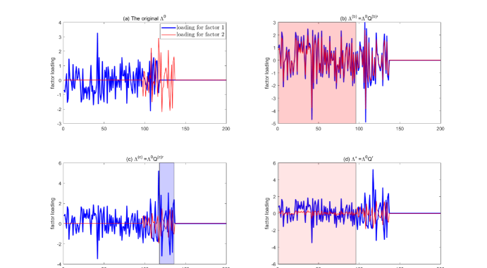
Figure 1: Illustration of sparsity degree preservation by PC rotation

Part (a) of Figure 1 shows underlying $\Lambda^{0}$ in which $\mathcal{L}_{1}^{0}=\{i:i=1,\ldots,117\}$, and $\mathcal{L}_{2}^{0}=\{i:i=97,\ldots,136\}$. The rotation matrix is calculated as $Q=\left(\begin{array}[]{rr}-1.07&1.46\\ -0.19&-0.67\end{array}\right).$ Panel (b) illustrates a common concern that $\Lambda^{0}$ rotated by an arbitrary nonsingular matrix, say $Q^{(b)}$, would become less sparse. To make an example, we randomly generate each element of $Q^{(b)}$ as $\mathcal{N}(0,1)$ so that $Q^{(b)}=\left(\begin{array}[]{rr}-1.44&-0.98\\ -1.16&-0.75\end{array}\right)$. It is obvious in part (b) that $\mathcal{L}_{2}^{0}$ is “inflated” considerably (by the shaded area) such that the two factors turn out to have the same strength. Part (c) displays the rotation effect by a stylized exactly upper triangular matrix $Q^{(c)}$. $Q^{(c)}$ here is set the same as $Q$ except $Q_{21}^{(c)}=0$, i.e., $Q^{(c)}=\left(\begin{array}[]{cc}-1.07&1.46\\ 0&-0.67\end{array}\right)$. Clearly, the upper triangular $Q^{(c)}$ resolves inflation to $\mathcal{L}_{2}^{0}$. On the other hand, we see in part (c) that $\mathcal{L}_{1}^{0}$ is somewhat inflated due to the loading on $\{i:i=118,\ldots,136\}$ (by the shaded area) from factor 2. Nevertheless, the distortion is much less severe and negligible relative to factor 1’s pervasiveness, since factor 2 is relatively weak. Finally, part (d) displays $\Lambda^{\ast}$ rotated by the real $Q$ in the simulation. The absolute value of $Q_{21}$ is indeed very small as expected in a finite sample ($Q_{21}\asymp_{p}200^{-0.2}$), though it is not exactly 0. By virtue of this feature, the inflated part of $\Lambda_{\cdot,2}^{\ast}$ (by the shaded area) is uniformly small and vanishing at a certain rate, which will be screened off together with estimation errors to reveal sparsity. We formalize the idea in the next subsection.

4.2 Sparsity recovery with PC estimators

Our previous analysis in subsection 4.1 provides a positive identification result for $\Lambda^{\ast}$ rotated by $Q$. In practice, $\Lambda^{\ast}$ is not observable, and the available is the PC estimator $\widetilde{\Lambda}$. In this subsection, we will present how the recovery of sparsity, not just its degree, is achieved by working with $\widetilde{\Lambda}$. Undoubtedly we need to take into account of the estimation error consisting of $\widetilde{\lambda}_{i}-\lambda_{i}^{\ast}=T^{-1}H^{\prime}F^{0\prime}e_{i}+T^{-1}(\widetilde{F}-F^{0}H)^{\prime}e_{i}$. Theorem 3.10 (i) lends us a hand stating that the estimation errors are also uniformly vanishing, and thus justifies the sparsity recovery via screening the PC estimator $\widetilde{\lambda}_{i}$.

We shall show that the set $\mathcal{L}_{k}^{0}=\{i:\lambda_{ik}^{0}\neq 0\}$ characterizing sparsity for factor $k$ can be recovered well approximately with regulated PC estimators. When the absolute value of $\widetilde{\lambda}_{ik}$ is small, we can set the factor loading as 0. So we choose the non-zero factor loadings with a threshold value $c_{\lambda,NT}$:

$$\widehat{\lambda}_{ik}=\widetilde{\lambda}_{ik}\mathbf{1}\left\{\left|\widetilde{\lambda}_{ik}\right|>c_{\lambda,NT}\right\}\ \text{where }c_{\lambda,NT}=\frac{1}{\sqrt{\ln\left(NT\right)}}.\text{ }$$

Similarly define the estimated non-zero set for the $k$th factor loading by $\widehat{\mathcal{L}}_{k}=\{i:\widehat{\lambda}_{ik}\neq 0\}.$ To evaluate the sparsity recovery accuracy of $\widehat{\mathcal{L}}_{k}$, we denote the symmetric difference between the true non-zero set $\mathcal{L}_{k}^{0}$ and its estimator $\widehat{\mathcal{L}}_{k}$ by

$$\mathcal{L}_{k}^{0}\triangle\widehat{\mathcal{L}}_{k}=\left(\mathcal{L}_{k}^{0}\backslash\widehat{\mathcal{L}}_{k}\right)\cup\left(\widehat{\mathcal{L}}_{k}\backslash\mathcal{L}_{k}^{0}\right).$$

We present the main results on sparsity recovery of factor loadings in the following Proposition.

Proposition 4.1

Under Assumptions 1-9, for $k=1,\ldots,r$, we have:

(i) if $\alpha_{k}$ is unique in $\{\alpha_{1},\alpha_{2},\ldots,\alpha_{r}\}$, then

$$\frac{\lvert\mathcal{L}_{k}^{0}\triangle\widehat{\mathcal{L}}_{k}\rvert}{N^{\alpha_{k}}}=o_{p}(1);$$

(ii) if $\alpha_{k}$ is not unique in $\{\alpha_{1},\alpha_{2},\ldots,\alpha_{r}\}$, then

$$\frac{\lvert\mathcal{L}_{k}^{0}\triangle\widehat{\mathcal{L}}_{k}\rvert}{N^{\alpha_{k}}}=O_{p}(1).$$

Remark 10. The approximation of sparsity for the $k$th factor is characterized by bounding the symmetric difference between $\mathcal{L}_{k}^{0}$ and $\widehat{\mathcal{L}}_{k}$ ($\mathcal{L}_{k}^{0}\triangle\widehat{\mathcal{L}}_{k}$) well relative to its factor strength. In particular, the $k$th factor’s sparsity, measured in $\mathcal{L}_{k}^{0}$, is recovered consistently relatively to its pervasiveness when $\alpha_{k}$ is unique; when $\alpha_{k}$ is not unique, the difference $\mathcal{L}_{k}^{0}\triangle\widehat{\mathcal{L}}_{k}$ is still well bounded relatively—a condition implying consistency of the factor strength estimator in Section 4.3.

Remark 11. (i) In the sparsity recovery of factor loadings, $c_{\lambda,NT}$ plays the key role of screening off noises due to rotation and estimation errors that are negligible in size. We show that the noises are $O_{p}\left(N^{-\zeta}+\left[(\ln N)/T\right]^{1/2}\right)$ uniformly, where $\zeta=\min_{1\leq k\leq G-1}\left(\alpha_{[k]}-\alpha_{[k+1]}\right),$ i.e., the minimum discrepancy between distinct factor strengths. So we set $c_{\lambda,NT}=\left[\ln\left(NT\right)\right]^{-1/2}$ to dominate the noise. (ii) Alternatively, We can consider an alternative threshold value $\widetilde{c}_{\lambda,NT}=c\left[\ln\left(NT\right)\right]^{-1/2}$ with a tuning parameter $c$. The optimal value of $c$ can be determined by some adaptive methods such as cross validation. Given that each (time) series will be demeaned and standardized to have unit variance, as recommended by Bai and Ng (2002), we focus on the simple threshold $c_{\lambda,NT}$. In both simulations and the empirical application, our tuning parameter-free threshold value $c_{\lambda,NT}$ works reasonably well. (iii) The choice of a threshold value simply by the relevant dominant rate is also adopted in Fan et al. (2015) to construct a screening statistic.

Figure 2 shows the intuition behind Proposition 4.1 using a three-factor model. By the path from part (a) to (b) and then to (c), we see that the distortion to model sparsity by rotation and estimation errors is either (i) dominated in absolute values relative to our screening threshold $c_{\lambda,NT}$, or (ii) negligible in size relative to factor pervasiveness. Consequently, sparsity is well approximated by regulation in part (d).

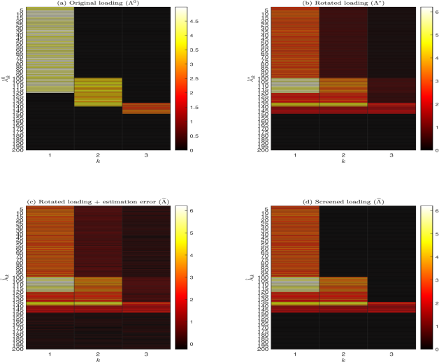
Figure 2: Illustration of the loading sparsity revelation

Note that Uematsu and Yamagata’s (2023a) SOFAR estimator recovers sparsity alternatively by $\ell_{1}$ regularization. Interestingly, if we contrast the estimate of factor loadings by PC (their Figures 7 and 2) with that by SOFAR (their Figures 9 and 11) in their empirical results, we immediately realize that PC and SOFAR estimates are almost identical, except for many small noises introduced by PC. This observation suggests the validity of combining PC estimate with proper screening to recover sparsity, which in fact underlines the method used in our paper.

4.3 Estimating factor strengths

BKP (2021) consider the pervasiveness of the unobserved macroeconomic shocks by using the estimated factor strength. They can only identify and estimate the strength of the strongest factor, and the results are thus limited. We can consistently estimate factor strengths for all weak factors with various strengths, which helps understand pervasiveness of factors completely. We hope that our proposed estimator of factor strength is of independent interest.

We can understand how influential each factor is by studying to its strength. Recall that $\alpha_{k}$ is such that $\sum_{i=1}^{N}\lambda_{ik}^{0\prime}\lambda_{ik}^{0}\asymp N^{\alpha_{k}}.$ Now for $k=1,...,r,$ define

$$\widehat{D}_{k}=\sum_{i=1}^{N}\mathbf{1}\left\{\left|\widetilde{\lambda}_{ik}\right|>c_{\lambda,NT}\right\},$$

where $c_{\lambda,NT}=\left[\ln\left(NT\right)\right]^{-1/2}$ as before. Our estimator for $\alpha_{k}$ is simply

$$\widehat{\alpha}_{k}=\frac{\ln\widehat{D}_{k}}{\ln N}.$$

To consistently estimate all factor strengths, one additional restriction is needed. Define

$$\Theta(\Lambda^{0})=\left\{\Lambda:\Lambda=\Lambda^{0}R,\;\text{for a fixed nonsingular $r\times r$ matrix $R$}\right\}.$$

Assumption 10. $\forall\breve{\Lambda}\in\Theta(\Lambda^{0})$, $\|\breve{\Lambda}_{\cdot,k}\|_{0}\leq\|\Lambda_{\cdot,k}\|_{0}+M$, for some constant $M<\infty$.

The above assumption implies that $\Lambda^{0}$ is the sparsest representation, up to a constant, among all observationally equivalent loading matrices. $\Lambda^{0}$ is of most interest as it provides the most concise interpretation of latent factors. Assumption 10 excludes, for instance, two factors with highly correlated loadings.

Theorem 4.2

Under Assumptions 1-10, for $k=1,...,r,$ $\widehat{\alpha}_{k}\overset{p}{\rightarrow}\alpha_{k}.$

Remark 12. Theorem 4.2 shows that our proposed estimator can consistently estimate strengths for all factors, not just for the strongest one as in BKP (2021). The intuition behind this consistency result is similar to that behind Proposition 4.1. Again, the key is to realize that the rotated loading matrix $\Lambda_{\cdot,k}^{0\ast}$ is able to preserve strength as $\alpha_{k}$ up to the given threshold $c_{\lambda,NT}$, and also that the errors induced by estimation are also uniformly dominated by $c_{\lambda,NT}$.

5 The Determination of the Number of Factors

The determination of the number of factors has been of long-standing interest in the literature of factor models. Various selection criteria have been proposed, e.g., Bai and Ng (2002), Onatski (2010), Ahn and Horenstein (2013), and Wei and Chen (2020). As for consistent selection in weak factor models, Uematsu and Yamagata (2023a) show that the edge distribution (ED) estimator by Onatski (2010) is consistent, and Onatski (2015) proposes selecting the number of factors based on the approximations to the squared error of the least squares estimator of the common component under both strong and weak factors asymptotics. Freyaldenhoven (2022a) devises a statistic in combining both eigenvalues and eigenvectors of the covariance matrix, to enhance its discriminatory power in distinguishing factors stronger than a certain threshold, assuming that $N$ and $T$ grows proportionally. Guo et al. (2022) exploit a data-driven adaptive penalty of factor strength for information criteria, to select weak factors and meanwhile avoid overfitting.

In this paper, we propose determining the number of factors based on SVT, as discussed by Bai and Ng (2019) and Freyaldenhoven (2022a). The procedure is very simple and works in the same spirit as Bai and Ng (2002). To determine the number of factors in $F^{0}$, we use the following estimator of $r$,

$$\widehat{r}=\max\left\{k:\widetilde{V}_{k}^{r_{\max}}\geq C_{r}\widehat{\sigma}^{2}N^{-1/2}\left(\ln\ln N\right)^{1/2}\right\},$$

where $\widehat{\sigma}^{2}$ is a consistent estimator of $(NT)^{-1}\sum_{i=1}^{N}\sum_{t=1}^{T}E\left(e_{it}^{2}\right)$, $C_{r}$ is a constant independent of $N$ and $T$, $r_{\max}$ is a large bounded positive integer such that $r\leq r_{\max}$, and $\widetilde{V}_{k}^{r_{\max}}$ is the $k$th diagonal element of $\widetilde{V}^{r_{\max}}\equiv\operatorname{diag}\left(\widetilde{V}_{1},\ldots,\widetilde{V}_{r_{\max}}\right)$ being an $r\times r$ diagonal matrix consisting of the $r_{\max}$ largest eigenvalues of $X^{\prime}X/(NT)$ in decreasing order. As for $\widehat{\sigma}^{2}$ in practice, we compute it similar to Bai and Ng (2002) as $\widehat{\sigma}^{2}=\frac{1}{NT}\sum_{i=1}^{N}\sum_{t=1}^{T}\left(X_{it}-\widetilde{\lambda}_{i}^{r_{\max}\prime}\widetilde{F}_{t}^{r_{\max}}\right)^{2}$, where the superscript $r_{\max}$ signifies the allowance of $r_{\max}$ factors in the estimation.

Remark 13. To implement, we choose the value of $C_{r}$ via twice K-fold cross validation as proposed by Wei and Chen (2020). Specifically, for a given $C_{r}$ and the consequent estimator of $r$, in step one we run a “leave one of $K$ folds out” (across columns of $X$) estimation by PC to obtain estimated loadings for all $N$ units, which are then sparsified by $c_{\lambda,NT}$. In step two we further run a “leave one of $J$ folds out” (across rows of $X$) estimation based on the fold left over from step one, to obtain estimated factors. Lastly, we evaluate the performance of estimation by out-of-sample mean squared errors averaged over all possible folds, and choose the $C_{r}$ to minimize the average. One can refer to Wei and Chen (2020) for implementation details. In practice, we choose $J=K=5$ and find the results are very robust against various values of $J$ and $K$.

Theorem 5.1

Under Assumptions 1-7, $\widehat{r}\overset{p}{\rightarrow}r.$

Remark 14. Proving Theorem 5.1, detailed in the Appendix, is to check two conditions to hold in probability: (i) $\widehat{r}\geq r$ and (ii) $\widehat{r}\leq r.$ Condition (i) is actually implied by Proposition 3.1. We prove condition (ii) by contradiction, and this relies on a sharper bound obtained under $\left\|e\right\|_{sp}^{2}=O_{p}\left(\max\left\{N,T\right\}\right)$ imposed by Assumption 4. This assumption is also needed for Bai and Ng (2002) in determining the number of factors via information criteria even in strong factor models.

Remark 15. The ED estimator proposed by Onatski (2010) is based on the fact that all the “systematic” eigenvalues diverge to infinity, whereas any finite number of the largest “idiosyncratic” eigenvalues cluster around a single point. Onatski (2010) determines the number of factors by separating the diverging eigenvalues with a wedge $\delta$, and proves the consistency of the ED estimator only requiring that $\min_{1\leq k\leq r}\alpha_{k}>0$. However, the ED estimator hinges on the idiosyncratic terms being guassian, or independent cross-sectionally or over time in case of nonguassian, and is thus restrictive in applications with macroeconomics and finance. As for choosing $\delta$, Onatski (2010) approximates the upper bound of eigenvalue differences by an OLS estimate which is then doubled to formulate $\delta$. His final estimator of $r$ is obtained via iterations given $\delta$. In contrast, our estimator of $r$ is more straightforward to use.

6 Monte Carlo Simulations

In this section, we study the finite sample performance of our proposed estimators for sparsity-induced weak factor models. It includes comparison of simple PC estimators with Lasso type estimators, estimation of number of factors, as well as factor strength.

6.1 The data generating process

We consider the following data generating process (DGP):

$$X_{it} = \lambda_{i}^{0\prime}F_{t}^{0}+e_{it},\text{ }i=1,...,N,\text{ }t=1,...,T$$

$$F_{1t}^{0} = 0.5F_{1,t-1}^{0}+u_{1t},\text{ and }F_{kt}^{0}=\left(-0.8\right)^{k}F_{1t}^{0}+u_{kt},\text{ }k=2,...,r$$

The simulated factors are correlated with each other with various degrees. We let $u_{kt}$ be mutually uncorrelated $\mathcal{N}\left(0,1\right)$ for $k=1,...,r$. To specify the factor loadings $\lambda_{ik}^{0},$ for each $k=1,...,r,$ we first randomly select $\lfloor N^{\alpha_{k}}\rfloor$ of $\left\{\lambda_{ik}^{0}\right\}_{i=1}^{N}$ and specify them as iid $\mathcal{N}\left(0,1\right)$, and then set the rest of $\left\{\lambda_{ik}^{0}\right\}_{i=1}^{N}$ as zero.

For the $N\times 1$ vector $e_{t},$ we specify the (marginal) distribution of $e_{it}$ as the student-$t\left(5\right)$ to allow for heavy tail. The cross sectional dependence across $e_{it}$ is admitted through the $N\times N$ covariance matrix $\Sigma_{e}$ as follows. $\Sigma_{e}=\operatorname{diag}\left\{\Sigma_{1},...,\Sigma_{N/4}\right\}$ as a block-diagonal matrix with $4\times 4$ blocks located along the main diagonal. Each $\Sigma_{i}$ is assumed to be $I_{4}$ initially. We then randomly choose $\lfloor N^{0.3}\rfloor$ blocks among them and make them non-diagonal by setting $\Sigma_{i}\left(m,n\right)=0.5^{\left|m-n\right|}$. The design of cross sectional dependence follows Fan et al. (2015) except that the dependence is stronger here.

We have tried simulations with the number of factors $r=3$ and $5.$ For $r=3,$ we set $\alpha=\left(0.9,0.75,0.6\right);$ while for $r=5,$ we set $\alpha=\left(1,0.9,0.8,0.7,0.6\right)$. The number of simulations is 2000.

6.2 Simulation results

We first compare different methods to determine the number of factors with ours (WZ). The alternative selection rules range from the $IC_{p1}$ by Bai and Ng (2002, BN), Guo et al. (2022, GCT), Freyaldenhoven (2022b, FR), ED by Onatski (2010), and Ahn and Horenstein (2013, AH). $r_{\max}$ is set to be 8 if needed. The root mean square error (RMSE) and bias of the estimated number of factors by each method are reported in Tables 1 and 2. It is obvious that GCT, FR and AH are all subject to overestimation of $r$ in the presence of weak factors. ED and BN are not very bad but they are outperformed by our proposed method, since they tend to over- and under-estimate $r$, respectively. The ED estimator is not as effective as found previously in weak factor models, e.g., by Uematsu and Yamagata (2023a), implying that the ED performance may be sensitive to the choice of the wedge parameter $\delta$, as remarked in Section 5. Our proposed estimator of factor numbers is outstanding against all alternatives at all sample sizes.

Table 1: Estimating the number of factors when $r=3$

		RMSE							Bias
$N$	$T$	WZ	BN	GCT	FR	ED	AH		WZ	BN	GCT	FR	ED	AH
100	100	0.273	0.673	0.939	1.962	0.400	1.998		-0.059	-0.443	-0.882	-1.943	0.030	-1.998
	200	0.132	0.446	0.866	1.964	0.425	1.999		-0.011	-0.190	-0.748	-1.945	0.090	-1.999
	400	0.084	0.314	0.783	1.978	0.964	1.998		-0.006	-0.095	-0.611	-1.968	0.330	-1.997
200	100	0.102	0.600	0.916	1.973	0.284	2.000		-0.002	-0.355	-0.839	-1.955	0.059	-2.000
	200	0.055	0.241	0.739	1.952	0.354	2.000		-0.001	-0.056	-0.543	-1.909	0.075	-2.000
	400	0.000	0.120	0.445	1.952	0.448	1.999		0.000	-0.010	-0.180	-1.909	0.091	-1.998
400	100	0.081	0.687	0.932	1.946	0.244	2.000		0.004	-0.468	-0.870	-1.895	0.058	-2.000
	200	0.000	0.180	0.610	1.767	0.248	2.000		0.000	-0.032	-0.370	-1.562	0.057	-2.000
	400	0.000	0.039	0.209	1.584	0.297	1.997		0.000	0.001	-0.011	-1.255	0.061	-1.995

Table 2: Estimating the number of factors when $r=5$

		RMSE							Bias
$N$	$T$	WZ	BN	GCT	FR	ED	AH		WZ	BN	GCT	FR	ED	AH
100	100	0.273	0.742	2.708	3.975	0.455	4.000		-0.060	-0.499	-2.654	-3.962	-0.032	-4.000
	200	0.122	0.443	2.408	3.970	0.362	4.000		-0.014	-0.190	-2.321	-3.950	0.059	-4.000
	400	0.081	0.305	2.114	3.981	0.803	4.000		-0.006	-0.089	-2.011	-3.970	0.230	-4.000
200	100	0.120	0.590	2.465	3.960	0.278	4.000		-0.001	-0.333	-2.387	-3.925	0.052	-4.000
	200	0.059	0.228	1.843	3.909	0.254	4.000		-0.001	-0.046	-1.749	-3.822	0.049	-4.000
	400	0.032	0.095	1.371	3.911	0.257	3.998		-0.001	-0.007	-1.289	-3.826	0.041	-3.996
400	100	0.087	0.640	2.299	3.800	0.239	4.000		0.006	-0.404	-2.220	-3.610	0.052	-4.000
	200	0.039	0.166	1.548	3.256	0.235	4.000		0.002	-0.025	-1.462	-2.650	0.051	-4.000
	400	0.022	0.045	1.051	2.889	0.249	3.996		0.001	0.001	-1.033	-2.085	0.054	-3.992

To study the finite sample performance of PC estimators under weak factor models, we compare PC regression with the sparse orthogonal factor regression (SOFAR) proposed by Uematsu and Yamagata (2023a, b), assuming the true number of factors to be known. Based on Lasso penalization on factor loadings for sparsity, Uematsu and Yamagata develop the Adaptive (Ada) SOFAR estimator. They later improve the SOFAR estimator by introducing the Debiased (Deb) SOFAR estimator to recover its asymptotic normality. Furthermore, they address the multiple testing problem of loading sparsity and construct the Resparsifed (Res) SOFAR estimator to fulfill FDR control. Note that the various SOFAR estimators proposed by Uematsu and Yamagata result from penalized regression which targets sparsity explicitly. Thus it seems natural to suggest that one should be better off using their approaches to deal with weak factor models than using PC. However, as we have mentioned before, the simple PC estimators enjoy a nice property of automatic sparsity recognition, so that PC could even outperform the complicated SOFAR.

To measure the performance of factor and loading estimators, we follow Doz et al. (2012) to use the trace statistics:

$$TR^{F}=\frac{\mathop{\mathrm{T}r}\left(F^{0\prime}\widetilde{F}\left(\widetilde{F}^{\prime}\widetilde{F}\right)^{-1}\widetilde{F}^{\prime}F^{0}\right)}{\mathop{\mathrm{T}r}\left(F^{0\prime}F^{0}\right)},\quad TR^{\Lambda}=\frac{\mathop{\mathrm{T}r}\left(\Lambda^{0\prime}\widetilde{\Lambda}\left(\widetilde{\Lambda}^{\prime}\widetilde{\Lambda}\right)^{-1}\widetilde{\Lambda}^{\prime}\Lambda^{0}\right)}{\mathop{\mathrm{T}r}\left(\Lambda^{0\prime}\Lambda^{0}\right)}.$$

We also report the root mean squared errors in estimating the common component $C_{it}$ (RMSE^C). All results are included in Tables 3 and 4. The Res estimator is under the FDR rate $q=0.1$. It is interesting to see that the PC estimators of factors and common components are almost always better than any of SOFAR type estimators. Although the Resparsifed SOFAR estimator for $\Lambda$ outperforms PC under bigger sample sizes, the margin is small. Recall that the SOFAR estimator are constructed under the restriction on the true DGP that $\Lambda^{0^{\prime}}\Lambda^{0}$ being diagonal and $F^{0^{\prime}}F^{0}/T=I_{r}$ (or $E(F^{0^{\prime}}F^{0}/T)=I_{r}$), which implies that the rotation matrix $H$ will be asymptotically $I_{r}$. However, the restriction is violated under our DGP with correlated underlying factors, which might account for the worse performance of SOFAR. In an additional experiment whose results are not reported here, we modify our DGP with factors being indeed independent, and find that the SOFAR estimators are much closer to or even outperforms the PC estimator in estimating factors evaluated by $TR^{F}$, though their $RMSE^{C}$ are still bigger in general. Hence regression by PC seems a better choice given its robustness and easy implementation.

Table 3: Estimation of factor models when $r=3$

		$TR^{F}$					$TR^{\Lambda}$					$RMSE^{C}$
$N$	$T$	PC	Ada	Deb	Res		PC	Ada	Deb	Res		PC	Ada	Deb	Res
100	100	0.924	0.898	0.909	0.909		0.718	0.622	0.709	0.713		0.973	1.020	1.005	1.005
	200	0.936	0.918	0.924	0.924		0.786	0.720	0.783	0.788		0.953	0.988	0.967	0.967
	400	0.943	0.935	0.938	0.938		0.830	0.806	0.833	0.837		0.948	0.970	0.958	0.957
200	100	0.955	0.934	0.942	0.942		0.745	0.647	0.765	0.786		0.886	0.941	0.894	0.893
	200	0.964	0.953	0.957	0.957		0.811	0.752	0.826	0.841		0.881	0.910	0.879	0.879
	400	0.969	0.964	0.966	0.966		0.852	0.838	0.861	0.871		0.872	0.892	0.877	0.877
400	100	0.969	0.951	0.956	0.956		0.750	0.660	0.767	0.803		0.813	0.866	0.820	0.818
	200	0.976	0.966	0.970	0.970		0.816	0.764	0.828	0.853		0.806	0.844	0.812	0.812
	400	0.980	0.975	0.977	0.977		0.858	0.846	0.864	0.879		0.802	0.822	0.805	0.804

Table 4: Estimation of factor models when $r=5$

		$TR^{F}$					$TR^{\Lambda}$					$RMSE^{C}$
$N$	$T$	PC	Ada	Deb	Res		PC	Ada	Deb	Res		PC	Ada	Deb	Res
100	100	0.946	0.919	0.922	0.922		0.774	0.685	0.769	0.766		1.612	1.653	1.620	1.622
	200	0.953	0.938	0.941	0.941		0.820	0.761	0.818	0.817		1.599	1.633	1.610	1.611
	400	0.956	0.948	0.950	0.950		0.844	0.814	0.845	0.845		1.594	1.615	1.603	1.603
200	100	0.969	0.947	0.949	0.949		0.794	0.699	0.796	0.800		1.500	1.574	1.527	1.529
	200	0.973	0.960	0.963	0.963		0.837	0.777	0.839	0.843		1.496	1.541	1.513	1.514
	400	0.976	0.969	0.971	0.971		0.860	0.829	0.862	0.864		1.497	1.516	1.500	1.501
400	100	0.980	0.961	0.963	0.963		0.798	0.704	0.804	0.816		1.438	1.497	1.444	1.446
	200	0.983	0.972	0.974	0.974		0.841	0.780	0.844	0.852		1.430	1.467	1.434	1.435
	400	0.985	0.979	0.980	0.980		0.866	0.833	0.867	0.872		1.425	1.447	1.428	1.429

We further investigate the estimated factor strength by various methods in Tables 5 and 6. All estimates become less accurate as the true strength degree decreases, as expected. It is admitted that our proposed strength estimate (PC+Screening) suffers more of overestimation with fairly weak factors, e.g., those with $\alpha_{k}=0.6$. Otherwise, our estimate is comparable to, and sometimes even better than, those from SOFAR which is designed deliberately for sparsity recovery, especially for strength $\alpha_{k}\in[0.7,0.9]$. The message here again delivers the usefulness of our factor strength estimator, which works reasonably well while avoids involving heavy computation as in SOFAR. Moreover, we find that SOFAR tends to underestimate the number of factors in our simulation, and hence the relative advantage of our estimate is conservative as we assume $r$ is known here.

Table 5: Estimation of factor strength when $r=3$ with $\alpha=\left(0.9,0.75,0.6\right)$

		RMSE				Bias
$N$	$T$	$\widehat{\alpha}_{1}$	$\widehat{\alpha}_{2}$	$\widehat{\alpha}_{3}$		$\widehat{\alpha}_{1}$	$\widehat{\alpha}_{2}$	$\widehat{\alpha}_{3}$
		Panel A: PC+Screening
100	100	0.014	0.047	0.138		0.000	0.006	0.100
	200	0.014	0.048	0.169		0.002	0.003	0.073
	400	0.014	0.049	0.208		0.003	0.007	0.048
200	100	0.010	0.048	0.126		0.002	0.028	0.111
	200	0.009	0.045	0.138		0.002	0.023	0.091
	400	0.009	0.045	0.166		0.004	0.026	0.075
400	100	0.007	0.053	0.114		0.002	0.044	0.101
	200	0.006	0.048	0.103		0.002	0.040	0.079
	400	0.006	0.052	0.115		0.003	0.042	0.065
		Panel B: SOFAR_Debiased
100	100	0.017	0.094	0.085		0.004	-0.060	-0.019
	200	0.023	0.065	0.106		0.019	0.028	0.067
	400	0.030	0.103	0.162		0.028	0.096	0.146
200	100	0.012	0.095	0.059		0.000	-0.071	-0.021
	200	0.017	0.052	0.084		0.014	0.025	0.062
	400	0.025	0.095	0.148		0.024	0.091	0.138
400	100	0.010	0.102	0.050		-0.004	-0.085	-0.033
	200	0.013	0.043	0.054		0.011	0.023	0.036
	400	0.020	0.088	0.114		0.019	0.086	0.105
		Panel C: SOFAR_Resparsified
100	100	0.024	0.067	0.095		0.020	0.044	0.064
	200	0.030	0.103	0.130		0.028	0.095	0.106
	400	0.036	0.137	0.179		0.035	0.135	0.164
200	100	0.017	0.062	0.096		0.015	0.057	0.085
	200	0.025	0.099	0.129		0.024	0.098	0.121
	400	0.031	0.130	0.162		0.031	0.129	0.157
400	100	0.013	0.057	0.090		0.012	0.054	0.081
	200	0.021	0.093	0.104		0.020	0.092	0.098
	400	0.027	0.123	0.140		0.026	0.123	0.136

Table 6: Estimation of factor strength when $r=5$ with $\alpha=\left(1,0.9,0.8,0.7,0.6\right)$

		RMSE						Bias
$N$	$T$	$\widehat{\alpha}_{1}$	$\widehat{\alpha}_{2}$	$\widehat{\alpha}_{3}$	$\widehat{\alpha}_{4}$	$\widehat{\alpha}_{5}$		$\widehat{\alpha}_{1}$	$\widehat{\alpha}_{2}$	$\widehat{\alpha}_{3}$	$\widehat{\alpha}_{4}$	$\widehat{\alpha}_{5}$
		Panel A: PC+Screening
100	100	0.036	0.045	0.041	0.076	0.156		-0.034	-0.035	0.020	0.050	0.111
	200	0.034	0.043	0.043	0.076	0.187		-0.033	-0.034	0.021	0.047	0.081
	400	0.033	0.040	0.043	0.078	0.223		-0.032	-0.030	0.023	0.045	0.058
200	100	0.031	0.032	0.047	0.083	0.139		-0.030	-0.023	0.035	0.065	0.115
	200	0.030	0.030	0.047	0.076	0.159		-0.029	-0.021	0.035	0.052	0.095
	400	0.029	0.027	0.049	0.076	0.172		-0.028	-0.018	0.037	0.053	0.079
400	100	0.027	0.020	0.053	0.089	0.117		-0.027	-0.009	0.045	0.077	0.101
	200	0.026	0.018	0.052	0.084	0.107		-0.026	-0.008	0.042	0.070	0.065
	400	0.025	0.015	0.053	0.082	0.124		-0.025	-0.006	0.044	0.067	0.051
		Panel B: SOFAR_Debiased
100	100	0.029	0.056	0.045	0.055	0.062		-0.027	-0.045	-0.009	0.003	0.021
	200	0.020	0.024	0.061	0.089	0.106		-0.019	0.000	0.050	0.077	0.088
	400	0.015	0.037	0.097	0.142	0.157		-0.013	0.033	0.093	0.136	0.144
200	100	0.027	0.055	0.041	0.046	0.046		-0.026	-0.047	-0.013	-0.016	0.018
	200	0.019	0.020	0.059	0.070	0.089		-0.018	0.002	0.048	0.058	0.076
	400	0.013	0.037	0.097	0.127	0.136		-0.013	0.035	0.094	0.123	0.127
400	100	0.027	0.053	0.039	0.045	0.031		-0.026	-0.048	-0.023	-0.031	-0.002
	200	0.018	0.017	0.051	0.051	0.061		-0.017	0.002	0.041	0.040	0.046
	400	0.012	0.039	0.095	0.107	0.103		-0.012	0.037	0.092	0.103	0.095
		Panel C: SOFAR_Resparsified
100	100	0.024	0.021	0.053	0.092	0.100		-0.023	0.003	0.043	0.080	0.084
	200	0.017	0.036	0.087	0.136	0.135		-0.016	0.033	0.082	0.130	0.122
	400	0.012	0.056	0.121	0.181	0.179		-0.011	0.055	0.119	0.178	0.168
200	100	0.022	0.018	0.048	0.081	0.098		-0.022	0.010	0.040	0.074	0.092
	200	0.016	0.039	0.076	0.116	0.115		-0.015	0.038	0.071	0.111	0.110
	400	0.011	0.058	0.111	0.163	0.153		-0.011	0.058	0.108	0.160	0.148
400	100	0.021	0.019	0.041	0.068	0.087		-0.021	0.016	0.034	0.063	0.085
	200	0.015	0.042	0.066	0.095	0.098		-0.014	0.041	0.062	0.092	0.095
	400	0.010	0.060	0.097	0.139	0.123		-0.010	0.059	0.095	0.137	0.121

7 Empirical Application

We apply our approach to explore potential weak factors on macroeconomic indicators. We use data from the FRED-QD as a quarterly database for macroeconomic research (McCracken and Ng, 2021). The original data set consists of 248 quarterly frequency series dating back to 1959:Q2. By disregarding series with missing observations, we end up with $N=181$ series. The series are classified into 13 groups: NIPA; Industrial Production; Employment and Unemployment; Housing; Inventories, Orders, and Sales; Prices; Earnings and Productivity; Interest Rates; Money and Credit; Household Balance Sheets; Exchange Rates; Stock Markets; and Non-Household Balance Sheets.

For each of the series used in our sample, after having made the decision that the series should be managed in levels or log-levels, the transformation codes are first and second differences based on whether the series is $I(0)$, $I(1$), or $I(2)$ tested and suggested by McCracken and Ng (2021). Due to the transformation, two initial observations are dropped so each series starts from 1959:$Q4$ actually. We also normalize each series to have zero mean and unit variance.

We depict the numbers of weak factors estimated by WZ, BN ($IC_{p1}$) and ED in Figure 3. The estimation is implemented under a rolling window scheme with length fixed at 120. The time on the x-axis denotes the right end point of the window interval. By WZ, the large panel is with five factors in most of the time considered here. There are a few windows taking four factors, in which BN also reports the same number. On the other hand, BN results in only three factors for the first half of rolling windows. For the second half, BN finds five factors in only a few window intervals. Onatski (2010) suggests that the ED method is expected to detect present weak factors. However, the result does not seem to agree with this: ED outputs three factors most of time, and the number may drop to two or even one at times. There are only three times when ED reports estimated factor numbers bigger than three.

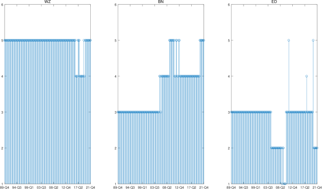
Figure 3: Estimated factor numbers by rolling windows

To have an idea of estimated factor strength and its dynamic, for each of our identified weak factors we further draw its associated factor strength over rolling windows in Figure 4 in a fashion similar to that in Figure 3. For most of window intervals ending from $1989$:$Q4$ to $2021$:$Q4$, we have five weak factors. Figure 4 demonstrates a clear sparsity structure of latent factors. The first two strongest factors seem to have very close strength around 0.8 most of the time, although $\widehat{\alpha}_{1}$ may spike to being close to 0.9 a few times. $\widehat{\alpha}_{3}$ ranges from 0.7 to 0.8. $\widehat{\alpha}_{4}$ fluctuates between 0.6 to 0.7, and interestingly it seems to spike simultaneously with $\widehat{\alpha}_{1}$, while reach bottom simultaneously with $\widehat{\alpha}_{3}$. $\widehat{\alpha}_{5}$ is around 0.6 and moves close to $\widehat{\alpha}_{4}$ up to 2014. However, $\widehat{\alpha}_{5}$ drops even to 0 (a reduced factor) during the last 6 years.

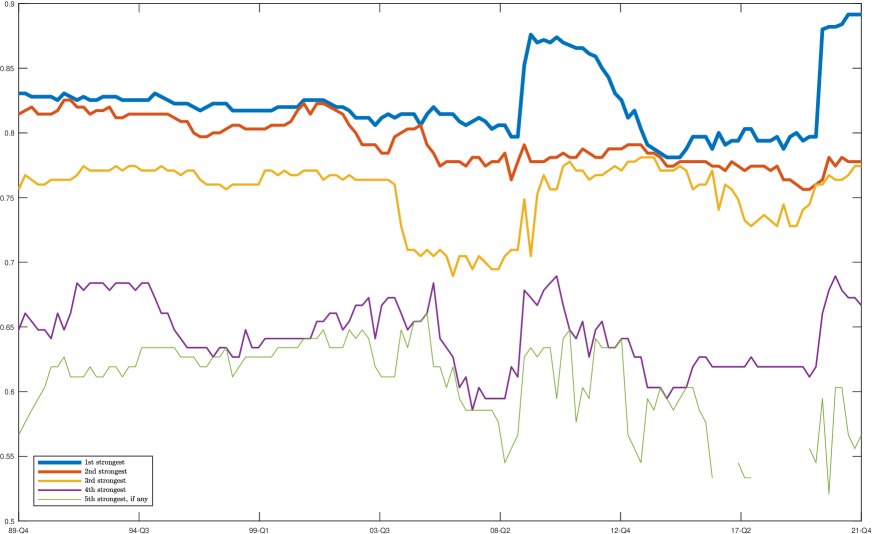
Figure 4: Estimated factor strength by rolling windows

We are also interested in factor pervasiveness in the cross sectional dimension, that is, what are those specific series exposed to each weak factor and the relative influence each factor exerts over space. We can infer the degree of influence roughly by looking at the sparsity of $\widehat{\lambda}_{ik}$ over $i$, given the implication by Proposition 4.1. We represent distribution of $\lvert\widehat{\lambda}_{ik}\rvert$ via a heat map of Figure 5. We consider two subperiods of roughly the same length: 1959:$Q3$-1989:$Q2$ and 1989:$Q3$-2021:$Q4$. For each subperiod, we detect 5 weak factors. Each row ($i$) represents a series and we add its associated group number ($\#1-\#13$) in front of its name. Each column ($k$) represents a principle component extracted as a latent factor, and we also signify its rank by factor strength. In particular, the estimated factor strengths are 0.831, 0.815, 0.756, 0.648, and 0.566 for 1959:$Q3$-1989:$Q2$, and 0.888, 0.784, 0.771, 0.654, 0.576 for 1989:$Q3$-2021:$Q4$, as put in the parenthesis. The darkness of each cell indicates the absolute value of $\widehat{\lambda}_{ik}$. Given that $\lvert\widehat{\lambda}_{ik}\rvert\leq 3$ mostly across $i$ and $k$, we right censor $\widehat{\lambda}_{ik}$ at 3 to obtain a sharper visualization of the heat map.

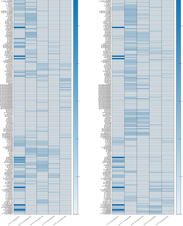
Figure 5: Heat map for recovered factor loading sparsity

Some interesting results are the following. While the top two factor strengths are close during the first subperiod, they move farther away from each other during the second subperiod. The rest of three factor strengths are fairly stable over the two subperiods. The 1st PC extracted as a factor is not necessarily the strongest one: it ranks the 3rd by the number of influenced series on the second subperiod. The 2nd PC ranks 2nd in strength in the first subperiod, yet rises to the 1st in strength in the second subperiod, as it is loaded by many new series most of which belong to group 6 (Prices). Meanwhile, the 3rd PC also gains additional influence, mostly from groups 1, 2 and 3 (NIPA; Industrial Production; Employment and Unemployment), giving rise to its incremental strength and rank enhancement, although it loses influence on a few series belonging to groups 8 (Interest Rates) and 10 (Household Balance Sheets). It may be also worth noticing that while some series are not influenced by any weak factors in subperiod 1, e.g., many of those from group 6, they start to load on some factors in subperiod 2.

8 Conclusion

This paper proposes a novel approach to deal with weak latent factor models with sparse factor loadings. It reveals an interesting and fundamental fact that the PC estimators can preserve the sparsity in estimated factor loadings for sparsity-induced weak factor models. This fact facilitates the derivation of asymptotic properties of PC estimators, enables us to recover the sparsity of loadings, and estimate the strengths of each factor. In addition, the determination of the number of factors in weak factor models is also investigated. The numerical studies confirm that our proposed approach works reasonably well in finite sample, and an empirical application to FRED-QD data set shows that our method is useful to detect factor strengths, loading sparsity and their dynamics.

Our estimators of weak factor models belong to unsupervised PCA. Conceptually, one could think of applying supervised PCA (e.g., Huang et al., 2022) to weak factor models and obtain more efficient results for estimation and inference. We agree that supervision would further improve the performance of our proposed estimators by better exploiting information available, and yet also raise up additional complexity. So we leave it to future research.

References

Abadir, K. and Magnus, J. (2005) Matrix Algebra. Cambridge University Press.

Ahn, S.C. and Horenstein, A.R. (2013) Eigenvalue ratio test for the number of factors. Econometrica, 81(3), 1203–1227.

Ando, T. and Bai, J. (2017) Clustering Huge Number of Financial Time Series: A Panel Data Approach With High-Dimensional Predictors and Factor Structures. Journal of the American Statistical Association, 112(519), 1182–1198.

Bai, J. (2003) Inferential theory for factor models of large dimensions. Econometrica, 71(1), 135–171.

Bai, J. and Ng, S. (2002) Determining the number of factors in approximate factor models. Econometrica, 70(1), 191–221.

Bai, J., and Ng, S. (2006). Confidence intervals for diffusion index forecasts and inference for factor-augmented regressions. Econometrica, 74(4), 1133-1150.

Bai, J. and Ng, S. (2019) Rank regularized estimation of approximate factor models. Journal of Econometrics, 212(1), 78–96.

Bai, J. and Ng, S. (2023) Approximate factor models with weaker loadings. Forthcoming at Journal of Econometrics.

Bailey, N., Kapetanios, G., and Pesaran, M.H. (2021) Measurement of factor strength: Theory and practice. Journal of Applied Econometrics, 36(5), 587–613.

Chao J.C., Liu, Y., and Swanson, N.R. (2022) Consistent factor estimation and forecasting in factor-augmented VAR models. Working Paper, Maryland University.

Chao J.C. and Swanson, N.R. (2022) Selecting the relevant variables for factor estimation in FAVAR models. Working Paper, Maryland University.

Choi, I., Lin, R., and Shin, Y. (2023) Canonical correlation-based model selection for the multilevel factors. Journal of Econometrics, 233(1), 22-44.

Doz, C., Giannone, D., and Reichlin, L. (2012) A quasi-maximum likelihood approach for large, approximate dynamic factor models. The Review of Economics and Statistics, 94(4), 1014–1024.

Despois, T. and Doz, C. (2022). Identifying and interpreting the factors in factor models via sparsity: Different approaches. Forthcoming at Journal of Applied Econometrics.

Fan, J., Liao, Y., and Mincheva, M. (2011) High-dimensional covariance matrix estimation in approximate factor models. Annals of Statistics, 39(6), 3320–3356.

Fan, J., Liao, Y., and Yao, J. (2015) Power enhancement in high-dimensional cross sectional tests. Econometrica, 83(4), 1497–1541.

Freyaldenhoven, S. (2022a) Factor models with local factors determining the number of relevant factors. Journal of Econometrics, 229(1), 80–102.

Freyaldenhoven, S. (2022b) Identification through sparsity in factor models: The $\ell_{1}$-rotation criterion. Working Paper, Federal Reserve Bank of Philadelphia.

Giglio, S. and Xiu, D. (2021) Asset pricing with omitted factors. Journal of Political Economy, 129(7), 1947–1990.

Giglio, S., Xiu, D., and Zhang, D. (2022a) Test assets and weak factors. Working Paper, NBER.

Giglio, S., Xiu, D., and Zhang, D. (2022b) Prediction when factors are weak. Working Paper, NBER.

Guo, X., Chen, Y., and Tang, C. Y. (2023) Information criteria for latent factor models: A study on factor pervasiveness and adaptivity. Journal of Econometrics, 233(1), 237-250.

Huang, D., Jiang, F., Li, K., Tong, G., and Zhou, G. (2022) Scaled PCA: A new approach to dimension reduction. Management Science, 68(3), 1678–1695.

Kristensen, J.T. (2017) Diffusion indexes with sparse loadings. Journal of Business & Economic Statistics 35(3), 434–451

Ludvigson, S.C. and Ng, S. (2009) Macro factors in bond risk premia. The Review of Financial Studies, 22(12), 5027-5067.

Ma, S., Linton, O., and Gao, J. (2021) Estimation and inference in semiparametric quantile factor models. Journal of Econometrics, 222(1), 295–323.

McCracken, M., and Ng, S. (2016). FRED-MD: A Monthly database for macroeconomic research. Journal of Business and Economic Statistics, 34(4), 574–589.

McCracken, M., and Ng, S. (2021). FRED-QD: A quarterly database for macroeconomic research. Federal Reserve Bank of St. Louis Review, 103(1), 1–44.

Merlevede, F., Peligrad, M., and Rio, E., (2011) A Bernstein type inequality and moderate deviations for weakly dependent sequences. Probability Theory and Related Fields, 151, 435–474

Moon, H.R. and Weidner, M. (2017) Dynamic linear panel regression models with interactive fixed effects. Econometric Theory, 33(1), 158–195.

Onatski, A. (2010) Determining the number of factors from empirical distribution of eigenvalues. The Review of Economics and Statistics, 92(4), 1004–1016.

Onatski, A. (2012) Asymptotics of the principal components estimator of large factor models with weakly influential factors. Journal of Econometrics, 168(2), 244–258.

Onatski, A. (2015) Asymptotic analysis of the squared estimation error in misspecified factor models. Journal of Econometrics, 186(2), 388–406.

Pelger, M. and Xiong, R. (2022) Interpretable Sparse Proximate Factors for Large Dimensions. Journal of Business and Economic Statistic, 40(4), 1642–1664.

Rapach, D. and Zhou, G. (2021) Sparse macro factors. Working paper, Washington University in St. Louis.

Stock, J.H. and Watson, M.W. (2002) Macroeconomic forecasting using diffusion indexes. Journal of Business & Economic Statistics, 20(2), 147–162.

Su, L. and Wang, X. (2017) On time-varying factor models: Estimation and testing. Journal of Econometrics, 198(1), 84–101.

Uematsu, Y. and Yamagata, T. (2023a) Estimation of sparsity-induced weak factor models. Journal of Business & Economic Statistics, 41(1), 126–139.

Uematsu, Y. and Yamagata, T. (2023b) Inference in sparsity-induced weak factor models. Journal of Business & Economic Statistics, 41(1), 213–227.

Wei, J., and Chen, H. (2020) Determining the number of factors in approximate factor models by twice K-fold cross validation. Economics Letters, 191, 109149.

APPENDIX

(Online)

The appendix provides formal proofs of main results in Sections 3-5 as well as auxiliary lemmas. We will use the fact that $\|B\|_{sp}\leq\|B\|_{F}\leq\|B\|_{sp}\mathop{\mathrm{r}ank}(B)^{1/2}$ over several places in our proofs.

Appendix A Proofs of the main results in Section 3

To start with, we present several useful lemmas which will be used frequently in the proofs of main results. Their proofs can be found in Section D.

Lemma A.1

Under Assumptions 1-5, $\Xi=\widetilde{V}^{-1}QAN^{-1}$ is a full rank (block) lower triangular matrix, and $\Xi=O_{p}(1).$

Lemma A.2

Under Assumptions 1-5, $\frac{1}{NT}\left\|e^{\prime}\Lambda^{0}F^{0\prime}\widetilde{F}\widetilde{V}^{-1}\right\|=O_{p}\left(N^{-\frac{\alpha_{r}}{2}}T^{\frac{1}{2}}\right).$

Lemma A.3

Under Assumptions 1-5, $\frac{1}{NT}ee^{\prime}\Lambda^{0}F^{0\prime}\widetilde{F}\widetilde{V}^{-1}=A^{-\frac{1}{2}}O_{p}(N+T).$

Lemma A.4

Under Assumptions 1-5, the $r\times r$ matrix $G\equiv F^{0\prime}\widetilde{F}/T$ is of full rank $r$ in probability.

Next we provide the proofs for the main results on PC estimator.

Proof of Proposition 3.1. Given $X=\Lambda^{0}F^{0\prime}+e,$ we get

$$\frac{1}{NT}X^{\prime}X=\frac{1}{NT}F^{0}\Lambda^{0\prime}\Lambda^{0}F^{0\prime}+\frac{1}{NT}F^{0}\Lambda^{0\prime}e+\frac{1}{NT}e^{\prime}\Lambda^{0}F^{0\prime}+\frac{1}{NT}e^{\prime}e.$$

Multiplying both sides by $N/N^{\alpha_{r}}$,

$$\frac{1}{N^{\alpha_{r}}T}X^{\prime}X=\frac{1}{N^{\alpha_{r}}T}F^{0\prime}\Lambda^{0\prime}\Lambda^{0}F^{0\prime}+\frac{1}{N^{\alpha_{r}}T}F^{0}\Lambda^{0\prime}e+\frac{1}{N^{\alpha_{r}}T}e^{\prime}\Lambda^{0}F^{0\prime}+\frac{1}{N^{\alpha_{r}}T}e^{\prime}e.$$

Note that the Frobenius norm of the second and third terms on the RHS is $o_{p}\left(1\right)$ as

$$\frac{1}{N^{\alpha_{r}}T}\left\|F^{0}\Lambda^{0\prime}e\right\| \leqslant \frac{1}{N^{\alpha_{r}}T}\left\|F^{0}\right\|\left\|\Lambda^{0\prime}e\right\|=\frac{1}{N^{\alpha_{r}}T}O_{p}\left(T^{\frac{1}{2}}\right)O_{p}\left(N^{\frac{\alpha_{1}}{2}}\right)$$

$$= O_{p}\left(N^{\frac{\alpha_{1}}{2}-\alpha_{r}}T^{-\frac{1}{2}}\right)=o_{p}(1).$$

This implies that

$$\frac{1}{N^{\alpha_{r}}T}\left\|F^{0}\Lambda^{0\prime}e\right\|_{sp}=\frac{1}{N^{\alpha_{r}}T}\left\|e^{\prime}\Lambda^{0}F^{0\prime}\right\|_{sp}=o_{p}(1).$$

For the fourth term,

$$\frac{1}{N^{\alpha_{r}}T}\left\|e^{\prime}e\right\|_{sp}=\frac{1}{N^{\alpha_{r}}T}O_{p}(N+T)=O_{p}\left(N^{1-\alpha_{r}}T^{-1}+N^{-\alpha_{r}}\right)=o_{p}(1).$$

Hence, the $r$ eigenvalues of $\frac{1}{N^{\alpha_{r}}T}X^{\prime}X$ are equal to the $r$ eigenvalues of $\frac{1}{N^{\alpha_{r}}T}F^{0}\Lambda^{0\prime}\Lambda^{0}F^{0\prime}$ in probability. Given that the eigenvalues of matrix $AB$ and those of $BA$ are identical, the $r$ eigenvalue of $\frac{1}{N^{\alpha_{r}}T}X^{\prime}X$ are determined in probability by

$$\left(\frac{1}{N^{\alpha_{r}}}\Lambda^{0\prime}\Lambda^{0}\right)\left(\frac{1}{T}F^{0\prime}F^{0}\right)=\frac{1}{N^{\alpha_{r}}}A^{1/2}\left(A^{-1/2}\Lambda^{0}\Lambda^{0}A^{-1/2}\right)A^{1/2}\left(\frac{1}{T}F^{0\prime}F^{0}\right).$$

By Assumptions 1-2, $A^{-1/2}\Lambda^{0\prime}\Lambda^{0}A^{-1/2}$ and $T^{-1}F^{0\prime}F^{0}$ are both converging to p.d. matrices. It follows that the $k$th eigenvalue of $\frac{1}{N^{\alpha_{r}}T}X^{\prime}X$

$$\mu_{k}\left(\frac{1}{N^{\alpha_{r}}T}X^{\prime}X\right)\asymp_{p}N^{-\alpha_{r}}A_{k}=N^{-\alpha_{r}}N^{\alpha_{k}},\text{ for }k=1,\cdots,r.$$

Thus,

$$\widetilde{V}_{k}=\mu_{k}\left(\frac{1}{NT}X^{\prime}X\right)\asymp_{p}N^{\alpha_{r}-1}N^{-\alpha_{r}}A_{k}=N^{\alpha_{k}-1},\text{ for }k=1,\cdots,r.\hskip 5.0pt\hbox{\hskip 5.0pt\vrule width=4.0pt,height=6.0pt,depth=1.5pt\hskip 1.0pt}$$

Proof of Proposition 3.2. For the so defined $G=F^{0\prime}\widetilde{F}/T,$ recall that we have already shown in proving Lemma A.4 that (a) $H$ is of full rank $r$ in probability, and (b) $H=O_{p}(1)$. Also recall that $\Sigma_{N,\Lambda}(k,k)\asymp N^{\alpha_{k}-1}$, $\Sigma_{N,\Lambda}(l,k)=O\left(N^{\alpha_{l\vee k}-1}\right)$, and $\widetilde{V}_{k}\asymp_{p}N^{\alpha_{k}-1}$. Hence for $H=\Sigma_{N,\Lambda}G\widetilde{V}^{-1}$ to hold with the asymptotic properties (a) and (b) just mentioned above, the $r\times r$ matrix $G$ must be such that

$$G(k,l)=O_{p}\left(N^{\alpha_{l}-\alpha_{k}}\right),\text{ for }1\leq k<l\leq r.$$

This clearly demonstrates that matrix $G$ is a (block) lower triangular matrix in probability. Specifically, for $1\leq k<l\leq r$ such that $\alpha_{l}<\alpha_{k},$ it must be that $G(k,l)=O_{p}\left(N^{\alpha_{l}-\alpha_{k}}\right)=o_{p}(1).$ Moreover, since $G$ is also of full rank of $r$ asymptotically as proved in Lemma A.4, we also have that $G(k,k)\asymp_{p}1$. Therefore, $G$ is a non-strictly (block) lower triangular matrix. Noticing that $Q=G^{\prime},$ we are done.     

Proof of Proposition 3.3. Note that

$$\widetilde{F}-F^{0}H=\left(\frac{F^{0}\Lambda^{0\prime}e\widetilde{F}}{NT}+\frac{e^{\prime}\Lambda^{0}F^{0\prime}\widetilde{F}}{NT}+\frac{e^{\prime}e\widetilde{F}}{NT}\right)\widetilde{V}^{-1}.$$

This implies

$$\frac{1}{\sqrt{T}}\left\|\widetilde{F}-F^{0}H\right\| \leq\left\{\left(\frac{\left\|F^{0}\right\|\|\widetilde{F}\|}{T}\right)\left(\frac{\left\|\Lambda^{0\prime}e\right\|}{\sqrt{T}N}\right)\left\|\widetilde{V}^{-1}\right\|+\frac{\left\|e^{\prime}\Lambda^{0}F^{0\prime}\widetilde{F}\widetilde{V}^{-1}\right\|}{NT\sqrt{T}}+\frac{\left\|e^{\prime}e\widetilde{F}\right\|}{NT^{3/2}}\left\|\widetilde{V}^{-1}\right\|\right\}$$

$$=O_{p}\left(\frac{\left\|\Lambda^{0\prime}e\right\|}{\sqrt{T}N}\left\|\widetilde{V}^{-1}\right\|\right)+O_{p}\left(\frac{\left\|e^{\prime}\Lambda^{0}F^{0\prime}\widetilde{F}\widetilde{V}^{-1}\right\|}{NT\sqrt{T}}\right)+O_{p}\left(\frac{\left\|e^{\prime}e\widetilde{F}\right\|}{NT^{3/2}}\left\|\widetilde{V}^{-1}\right\|\right).$$

Note that $\frac{1}{\sqrt{T}N}\left\|\Lambda^{0\prime}e\right\|=O_{p}\left(N^{\alpha_{1}/2-1}\right).$ Also, $\frac{\left\|ee^{\prime}\widetilde{F}\right\|}{NT^{3/2}}\leq\frac{\left\|ee^{\prime}\right\|_{sp}\|\widetilde{F}\|}{NT^{3/2}}=O_{p}\left(\frac{1}{N}\right)+O_{p}(\frac{1}{T}).$ Together with Lemma A.2 and Proposition 3.1, it leads to that

$$\frac{1}{T}\left\|\widetilde{F}-F^{0}H\right\|^{2}=O_{p}\left(N^{2\left(1-\alpha_{r}\right)}\right)O_{p}\left(N^{\alpha_{1}-2}+T^{-2}\right)=O_{p}\left(N^{\alpha_{1}-2\alpha_{r}}+N^{2\left(1-\alpha_{r}\right)}T^{-2}\right).\hskip 5.0pt\hbox{\hskip 5.0pt\vrule width=4.0pt,height=6.0pt,depth=1.5pt\hskip 1.0pt}$$

Proof of Proposition 3.4. First, note that

$$\widetilde{\Lambda}-\Lambda^{0}Q^{\prime}=\frac{1}{T}e\left(\widetilde{F}-F^{0}H\right)+\frac{1}{T}eF^{0}H.$$

Then let

$$L_{1} = \frac{1}{T}e\left(\widetilde{F}-F^{0}H\right)$$

$$= \left(\frac{1}{NT}ee^{\prime}\Lambda^{0}\right)\left(\frac{1}{T}F^{0^{\prime}}\widetilde{F}\right)\widetilde{V}^{-1}+\frac{1}{NT^{2}}eF^{0}\Lambda^{0\prime}e\widetilde{F}\widetilde{V}^{-1}+\frac{1}{NT^{2}}ee^{\prime}e\widetilde{F}\widetilde{V}^{-1}$$

$$\equiv L_{11}+L_{12}+L_{13}.$$

Note

$$L_{11}=\frac{1}{NT}\left(ee^{\prime}\right)\Lambda^{0}Q^{\prime}\widetilde{V}^{-1}=\frac{1}{NT}O_{p}(N+T)\left(\Lambda^{0}A^{-\frac{1}{2}}\right)\left(A^{-\frac{1}{2}}N\right)\left(AN^{-1}Q^{\prime}\widetilde{V}^{-1}\right).$$

By Assumption 2, $\left\|\Lambda^{0}A^{-\frac{1}{2}}\right\|=O\left(1\right).$ By Lemma A.1, $AN^{-1}Q^{\prime}\widetilde{V}^{-1}=O_{p}\left(1\right).$ So,

$$\left\|L_{11}\right\|\leq\frac{1}{NT}O_{p}(N+T)O_{p}\left(A^{-\frac{1}{2}}N\right)=O_{p}\left(N^{-\alpha_{r}}+N^{1-\frac{\alpha_{r}}{2}}T^{-1}\right).$$

Next for $L_{12},$ $L_{12}=\frac{1}{NT^{2}}\left(eF^{0}\right)\left(\Lambda^{0^{\prime}}eF^{0}H\right)\widetilde{V}^{-1}+\frac{1}{NT^{2}}eF^{0}\Lambda^{0^{\prime}}e\left(\widetilde{F}-F^{0}H\right)\widetilde{V}^{-1},$ so

$$\left\|L_{12}\right\|=\frac{1}{NT^{2}}O_{p}(\sqrt{NT})O_{p}\left(\sqrt{N^{\alpha_{1}}T}\right)O_{p}\left(N^{1-\alpha_{r}}\right)\left[1+O_{p}\|\widetilde{F}-F^{0}H\|\right]$$

Given that $\left\|\widetilde{F}-F^{0}H\right\|=O_{p}\left(\sqrt{TN^{\alpha_{1}-2\alpha_{r}}}+\sqrt{N^{2(1-2\alpha_{r})}T^{-1}}\right)$ by Proposition 3.3, we have

$$\left\|L_{12}\right\|=O_{p}\left(N^{\frac{\alpha_{1}}{2}-\alpha_{r}+\frac{1}{2}}T^{-1}+N^{\alpha_{1}-2\alpha_{r}+\frac{1}{2}}T^{-\frac{1}{2}}\right).$$

Lastly for $L_{13},$

$$\left\|L_{13}\right\|=\frac{1}{NT^{2}}\left\|e\right\|_{sp}^{3}O_{p}\left(T^{\frac{1}{2}}\right)O_{p}\left(N^{1-\alpha_{r}}\right)=O_{p}\left(T^{-\frac{3}{2}}N^{\frac{3}{2}-\alpha_{r}}+N^{-\alpha_{r}}\right).$$

Given Assumption 5$,\quad N^{\frac{3}{2}-\alpha_{r}}T^{-\frac{3}{2}}\ll N^{1-\frac{\alpha_{r}}{2}}T^{-1}.$ Also, it’s easy to see $N^{1-\frac{\alpha_{r}}{2}}\gg N^{\alpha_{1}-2\alpha_{r}+\frac{1}{2}}.$ So it follows that

$$L_{1}=O_{p}\left(N^{-\frac{\alpha_{r}}{2}}+N^{1-\frac{\alpha_{r}}{2}}T^{-1}+N^{\alpha_{1}-2\alpha_{r}+\frac{1}{2}}T^{-\frac{1}{2}}\right).$$ (A.1)

Meanwhile, as $T^{-1}eF^{0}H=O_{P}\left(N^{\frac{1}{2}}T^{-\frac{1}{2}}\right)$ implied by Assumption 3 (vii), and $H=O_{p}\left(1\right)$ as proved in Lemma A.4,

$$\left\|\widetilde{\Lambda}-\Lambda^{0}Q^{\prime}\right\|=O_{p}\left(N^{-\frac{\alpha_{r}}{2}}+N^{1-\frac{\alpha_{r}}{2}}T^{-1}+N^{\frac{1}{2}}T^{-\frac{1}{2}}\right)=O_{p}\left(N^{-\frac{\alpha_{r}}{2}}+N^{\frac{1}{2}}T^{-\frac{1}{2}}\right).$$

So we have $N^{-1}\left\|\widetilde{\Lambda}-\Lambda^{0}Q^{\prime}\right\|^{2}=O_{p}\left(N^{-\alpha_{r}-1}+T^{-1}\right).$   

Proof of Lemma 3.5. First, note that from $\frac{1}{NT}X^{\prime}X\widetilde{F}=\widetilde{F}\widetilde{V},$ we have $\frac{1}{NT}\left(\Lambda^{0}F^{0\prime}+e\right)^{\prime}(\Lambda^{0}F^{0\prime}+e)\widetilde{F}=\widetilde{F}\widetilde{V}.$ That is,

$$\widetilde{F}\widetilde{V}=\frac{1}{NT}F^{0}\Lambda^{0\prime}\Lambda^{0}\widetilde{F}+\frac{1}{NT}F^{0}\Lambda^{0\prime}e\widetilde{F}+\frac{1}{NT}e^{\prime}\Lambda^{0}F^{0\prime}\widetilde{F}+\frac{1}{NT}e^{\prime}e\widetilde{F}.$$

Thus, multiplying $\widetilde{F}^{\prime}/T$ on both sides of the above equation leads to

$$\widetilde{V}=\frac{1}{T}\widetilde{F}^{\prime}F^{0}\frac{1}{N}\Lambda^{0\prime}\Lambda^{0}\frac{1}{T}F^{0\prime}\widetilde{F}+\frac{1}{NT^{2}}\widetilde{F}^{{}^{\prime}}F^{0\prime}\Lambda^{0\prime}e\widetilde{F}+\frac{1}{NT^{2}}\widetilde{F}^{\prime}e^{\prime}\Lambda^{0}F^{0\prime}\widetilde{F}+\frac{1}{NT^{2}}\widetilde{F}^{\prime}e^{\prime}e\widetilde{F},$$

which gives rise to

$$I_{r} =QH+\frac{1}{NT^{2}}\widetilde{F}^{\prime}F^{0\prime}\Lambda^{0\prime}e\widetilde{F}\widetilde{V}^{-1}+\frac{1}{NT^{2}}\widetilde{F}^{\prime}e^{\prime}\Lambda^{0}F^{0\prime}\widetilde{F}\widetilde{V}^{-1}+\frac{1}{NT^{2}}\widetilde{F}^{\prime}e^{\prime}e\widetilde{F}\widetilde{V}^{-1}$$

$$\equiv QH+b_{1}+b_{2}+b_{3},\text{ say.}$$

It is easy to show that $b_{1}=O_{p}\left(N^{\frac{\alpha_{1}}{2}-1}\right)O_{p}\left(N^{1-a_{r}}\right)O_{p}\left(T^{-1/2}\right)=O_{p}\left(N^{\frac{\alpha_{1}}{2}-a_{r}}T^{-1/2}\right).$ The same result also holds for $b_{2}.$ Meanwhile,

$$b_{3}=O_{p}\left(1\right)\frac{1}{NT}\left\|e^{\prime}e\right\|_{sp}\widetilde{V}^{-1}=O_{p}\left(N^{-1}+T^{-1}\right)O_{p}\left(N^{1-a_{r}}\right)=O_{p}\left(N^{-a_{r}}+N^{1-a_{r}}T^{-1}\right).$$

So it follows that

$$I_{r}=QH+O_{p}\left(N^{\frac{\alpha_{1}}{2}-a_{r}}T^{-1/2}+N^{-a_{r}}+N^{1-a_{r}}T^{-1}\right)=QH+O_{p}\left(\gamma_{NT}\right),$$ (A.2)

implying that $Q=H^{-1}+O_{p}\left(\gamma_{NT}\right).$

Second, notice that (A.2) also implies that $H=Q^{-1}+O_{p}\left(\gamma_{NT}\right)=H_{3}+O_{p}\left(\gamma_{NT}\right).$

Third, recall by definition, $\widetilde{\Lambda}=\frac{1}{T}\Lambda^{0}F^{0^{\prime}}\widetilde{F}+\frac{1}{T}e\widetilde{F}.$ Therefore, we have

$$\frac{\Lambda^{0\prime}\widetilde{\Lambda}}{N}=\frac{\Lambda^{0\prime}\Lambda^{0}}{N}\frac{F^{0\prime}\widetilde{F}}{T}+\frac{\Lambda^{0\prime}e\widetilde{F}}{NT}.$$

So it is followed by

$$\left(\Lambda^{0\prime}\Lambda^{0}\right)^{-1}\Lambda^{0\prime}\widetilde{\Lambda}=F^{0\prime}\widetilde{F}/T+\left(\Lambda^{0\prime}\Lambda^{0}\right)^{-1}\Lambda^{0\prime}e\widetilde{F}/T=F^{0\prime}\widetilde{F}/T+\mathcal{R}_{1},$$

where $\mathcal{R}_{1}\equiv\left(\Lambda^{0^{\prime}}\Lambda^{0}\right)^{-1}\Lambda^{0\prime}e\widetilde{F}/T=\left(\Lambda^{0\prime}\Lambda^{0}A^{-1/2}\right)^{-1}A^{-1/2}\Lambda^{0\prime}e\widetilde{F}/T.$ We further note that $A^{-1/2}\Lambda^{0\prime}e\widetilde{F}/T=A^{-\frac{1}{2}}\Lambda^{0\prime}e(\widetilde{F}-F^{0}H)/T+A^{-\frac{1}{2}}\Lambda^{0\prime}eF^{0}H/T.$ It is followed by

$$\left\|A^{-1/2}\Lambda^{0\prime}e\widetilde{F}/T\right\| \leq \left\|A^{-\frac{1}{2}}\Lambda^{0\prime}e\right\|\left\|(\widetilde{F}-F^{0}H)/T\right\|+\left\|A^{-\frac{1}{2}}\Lambda^{0\prime}eF^{0}/T\right\|\left\|H\right\|$$

$$= O_{p}\left(N^{\frac{\alpha_{1}}{2}-\alpha_{r}}T^{-1/2}+N^{1-\alpha_{r}}T^{-\frac{3}{2}}\right)+O_{p}\left(T^{-1/2}\right)$$

$$= O_{p}\left(N^{\frac{\alpha_{1}}{2}-\alpha_{r}}T^{-1/2}+N^{1-\alpha_{r}}T^{-\frac{3}{2}}\right)=O_{p}\left(\gamma_{NT}\right).$$

The results above imply that $T^{-1}\widetilde{F}^{\prime}F^{0}=\widetilde{\Lambda}^{\prime}\Lambda^{0}\left(\Lambda^{0\prime}\Lambda^{0}\right)^{-1}+O_{p}\left(\gamma_{NT}\right).$ Again, recall the definitions that $Q=T^{-1}\widetilde{F}^{\prime}F^{0},$ and $H_{1}=\left(\Lambda^{0\prime}\Lambda^{0}\right)^{-1}\Lambda^{0\prime}\widetilde{\Lambda}$, together with $Q=H^{-1}+O_{p}\left(\gamma_{NT}\right)$ proved previously, we come to that $H_{1}=H+O_{p}\left(\gamma_{NT}\right).$

Fourth, notice immediately that $\Lambda^{0\prime}\widetilde{\Lambda}/N=\left(\Lambda^{0\prime}\Lambda/N\right)\left(F^{0\prime}\widetilde{F}/T\right)+\frac{1}{NT}\Lambda^{0\prime}e\widetilde{F}$, and we post-multiply $(\widetilde{\Lambda}^{\prime}\widetilde{\Lambda}/N)^{-1}$ on both sides of the equation, making use of $\widetilde{\Lambda}^{\prime}\widetilde{\Lambda}/N=\widetilde{V}$, to get that

$$H_{4} \equiv \left(\Lambda^{0\prime}\widetilde{\Lambda}\right)\left(\widetilde{\Lambda}^{\prime}\widetilde{\Lambda}\right)^{-1}$$

$$= H+\frac{1}{NT}\Lambda^{0\prime}e\widetilde{F}\left(\frac{1}{N}\widetilde{\Lambda}^{\prime}\widetilde{\Lambda}\right)^{-1}$$

$$= H+\left[\frac{1}{NT}\Lambda^{0\prime}e\left(\widetilde{F}-F^{0}H\right)+\frac{1}{NT}\Lambda^{0^{\prime}}eF^{0}H\right]O_{p}\left(N^{1-\alpha_{r}}\right)$$

$$= H+O_{p}\left(N^{\frac{\alpha_{1}}{2}-1}N^{\frac{\alpha_{1}}{2}-a_{r}}T^{-1/2}+N^{\frac{\alpha_{1}}{2}-1}N^{1-a_{r}}T^{-3/2}+N^{\frac{\alpha_{1}}{2}-1}T^{-1/2}\right)O_{p}\left(N^{1-\alpha_{r}}\right)$$

$$= H+O_{p}\left(N^{\frac{\alpha_{1}}{2}-a_{r}}T^{-1/2}\right)=H+O_{p}\left(\gamma_{NT}\right).$$

Lastly, to deal with $H_{2}$, we again start by definition

$$\widetilde{F}=\frac{1}{N}X^{\prime}\widetilde{\Lambda}\widetilde{V}^{-1}=\frac{1}{N}F^{0}\Lambda^{0\prime}\widetilde{\Lambda}\widetilde{V}^{-1}+\frac{1}{N}e^{\prime}\widetilde{\Lambda}\widetilde{V}^{-1}.$$

Now, if we pre-multiply $\frac{1}{T}F^{0\prime}$ on both sides, we get

$$\frac{1}{T}F^{0\prime}\widetilde{F} = \frac{1}{T}F^{0\prime}F^{0}\left(\frac{1}{N}\Lambda^{0\prime}\widetilde{\Lambda}\right)\widetilde{V}^{-1}+\frac{1}{NT}F^{0\prime}e^{\prime}\widetilde{\Lambda}\widetilde{V}^{-1}$$

$$= \left(\frac{1}{T}F^{0\prime}F^{0}\right)\left(\frac{1}{N}\Lambda^{0\prime}\widetilde{\Lambda}\right)\widetilde{V}^{-1}+\mathcal{R}_{2},$$

where

$$\mathcal{R}_{2} \equiv \frac{1}{NT}F^{0\prime}e^{\prime}\left(\widetilde{\Lambda}-\Lambda^{0}Q^{\prime}\right)\widetilde{V}^{-1}+\frac{1}{NT}F^{0\prime}e^{\prime}\Lambda^{0}Q^{\prime}\widetilde{V}^{-1}$$

$$= \frac{1}{NT}F^{0\prime}e^{\prime}\left(\widetilde{\Lambda}-\Lambda^{0}Q^{\prime}\right)\widetilde{V}^{-1}+\frac{1}{T}F^{0\prime}e^{\prime}\Lambda^{0}A^{-1}\left(AN^{-1}Q^{\prime}\widetilde{V}^{-1}\right)$$

$$= O_{p}\left(N^{-\frac{1}{2}}T^{-\frac{1}{2}}\right)O_{p}\left(N^{-\frac{\alpha_{r}}{2}}+N^{\frac{1}{2}}T^{-\frac{1}{2}}\right)O_{p}\left(N^{1-\alpha_{r}}\right)+O_{p}\left(N^{-\frac{\alpha_{r}}{2}}T^{-\frac{1}{2}}\right)$$

$$= O_{p}\left(N^{\frac{1}{2}-\frac{3}{2}\alpha_{r}}T^{-\frac{1}{2}}+N^{1-\alpha_{r}}T^{-1}\right)+O_{p}\left(N^{-\frac{\alpha_{r}}{2}}T^{-\frac{1}{2}}\right)=O_{p}\left(\gamma_{NT}\right),$$

and the third equality is by Theorem 3.4, Lemma A.1 and Assumption 3 (v). It follows that

$$\underbrace{\left(F^{0\prime}F^{0}\right)^{-1}F^{0\prime}\widetilde{F}}_{:=H_{2}}=\underbrace{\left(\Lambda^{0\prime}\widetilde{\Lambda}\right)\left(\widetilde{\Lambda}^{\prime}\widetilde{\Lambda}\right)^{-1}}_{:=H_{4}}+O_{p}\left(\gamma_{NT}\right).$$

Putting things together, we have shown (i) $H=H_{3}+O_{P}\left(\gamma_{NT}\right),$ (ii) $H_{1}=H+O_{p}\left(\gamma_{NT}\right),$ (iii) $H_{4}=H+O_{p}\left(\gamma_{NT}\right),$ (iv) $H_{2}=H_{4}+O_{p}\left(\gamma_{NT}\right).$ In all, we conclude that $H_{l}=H+O_{p}\left(\gamma_{NT}\right),$ $l=1,\cdots,4.$   

Proof of Proposition 3.6. Now we have

$$\frac{1}{NT}\left\|\widetilde{C}-C^{0}\right\|^{2} = \frac{1}{NT}\left\|\widetilde{\Lambda}\widetilde{F}^{\prime}-\Lambda^{0}H^{\prime-1}H^{\prime}F^{0\prime}\right\|^{2}$$

$$= \frac{1}{NT}\left\|\left(\widetilde{\Lambda}-\Lambda^{0}H^{\prime-1}+\Lambda^{0}H^{\prime-1}\right)\widetilde{F}^{\prime}-\Lambda^{0}H^{\prime-1}H^{\prime}F^{0\prime}\right\|^{2}$$

$$\leq \frac{2}{NT}\left\|\Lambda^{0}H^{\prime-1}\left(\widetilde{F}-F^{0}H\right)^{\prime}\right\|^{2}+\frac{2}{NT}\left\|\widetilde{\Lambda}-\Lambda^{0}H^{\prime-1}\right\|^{2}\|\widetilde{F}\|^{2}$$

$$= O_{p}\left(\frac{1}{N}\left\|\Lambda^{0}\right\|^{2}\right)O_{p}\left(\frac{1}{T}\left\|\widetilde{F}-F^{0}H\right\|^{2}\right)$$

$$+O_{p}\left(\frac{1}{N}\left\|\widetilde{\Lambda}-\Lambda^{0}Q^{{}^{\prime}}\right\|^{2}\right)+O_{p}\left(\left\|Q-H^{-1}\right\|^{2}\right)$$

$$= O_{p}\left(N^{\alpha_{1}-1}\right)O_{p}\left(N^{\alpha_{1}-2\alpha_{r}}+N^{2\left(1-\alpha_{r}\right)}T^{-2}\right)$$

$$+O_{p}\left(N^{-\alpha_{r}-1}+T^{-1}\right)+O_{p}\left(N^{\alpha_{1}-2\alpha_{r}}T^{-1}+N^{2\left(1-\alpha_{r}\right)}T^{-2}+N^{-2\alpha_{r}}\right)$$

$$= O_{p}\left(N^{2\left(\alpha_{1}-\alpha_{r}\right)-1}+T^{-1}\right).$$

The second last equality is due to Propositions 3.3, 3.4, and Lemma 3.5. The last equality is due to Assumption 5.    

Proof of Theorem 3.7. Let us start from the definition, $\widetilde{F}=\frac{1}{N}X^{\prime}\widetilde{\Lambda}\widetilde{V}^{-1}.$ Then by plugging $X=\Lambda^{0}F^{0\prime}+e,$ we get $\widetilde{F}=\frac{1}{N}F^{0}\Lambda^{0\prime}\widetilde{\Lambda}\widetilde{V}^{-1}+\frac{1}{N}e^{\prime}\widetilde{\Lambda}\widetilde{V}^{-1}.$ That is, $\widetilde{F}_{t}=H_{4}^{\prime}F_{t}^{0}+\widetilde{V}^{-1}\frac{1}{N}\widetilde{\Lambda}^{\prime}e_{t}$. So

$$\widetilde{F}_{t}-H_{4}^{\prime}F_{t}^{0}=\widetilde{V}^{-1}\frac{1}{N}\left(\widetilde{\Lambda}-\Lambda^{0}Q\right)^{\prime}e_{t}+\widetilde{V}^{-1}\frac{1}{N}Q\Lambda^{0\prime}e_{t}.$$

We first consider the first term on the RHS of the above equation.

$$\widetilde{V}^{-1}\frac{1}{N}\left(\widetilde{\Lambda}-\Lambda^{0}Q\right)^{\prime}e_{t}=\widetilde{V}^{-1}\frac{1}{N}\left[\frac{1}{T}e\left(\widetilde{F}-F^{0}H\right)\right]^{\prime}e_{t}+\widetilde{V}^{-1}\frac{1}{N}\left(\frac{1}{T}eF^{0}H\right)^{\prime}e_{t}\equiv W_{t}+Z_{t},\text{ say.}$$

For $W_{t},$ we have a further decomposition as

$$W_{t} = \widetilde{V}^{-1}\frac{1}{N}\left(\frac{eF^{0}\Lambda^{0\prime}e\widetilde{F}\widetilde{V}^{-1}}{NT^{2}}\right)^{\prime}e_{t}+\widetilde{V}^{-1}\frac{1}{N}\left(\frac{ee^{\prime}\Lambda^{0}F^{0\prime}\widetilde{F}\widetilde{V}^{-1}}{NT^{2}}\right)^{\prime}e_{t}+\widetilde{V}^{-1}\frac{1}{N}\left(\frac{ee^{\prime}e\widetilde{F}\widetilde{V}^{-1}}{NT^{2}}\right)^{\prime}e_{t}$$

$$\equiv W_{t}^{(a)}+W_{t}^{(b)}+W_{t}^{(c)},\text{ say.}$$

For $W_{t}^{(a)}=\frac{1}{N^{2}T^{2}}\widetilde{V}^{-2}\widetilde{F}^{\prime}e^{\prime}\Lambda^{0}F^{0\prime}e^{\prime}e_{t},$ we first have $\frac{1}{NT}F^{0\prime}e^{\prime}e_{t}=O_{p}\left(\left(NT\right)^{-1/2}+T^{-1}\right)$ by Assumption 3 (vi). Also recall that $\left\|e^{\prime}\Lambda^{0}\right\|=O_{p}\left(N^{\alpha_{1}/2}T^{1/2}\right).$ Hence,

$$W_{t}^{(a)} = \frac{1}{NT}\widetilde{V}^{-2}O_{p}\left(T^{\frac{1}{2}}\right)O_{p}\left(N^{\frac{\alpha_{1}}{2}}T^{\frac{1}{2}}\right)O_{p}\left(\frac{1}{\sqrt{NT}}+\frac{1}{T}\right)$$

$$= \widetilde{V}^{-2}O_{p}\left(N^{\frac{\alpha_{1}-3}{2}}T^{-\frac{1}{2}}+N^{\frac{\alpha_{1}}{2}-1}T^{-1}\right).$$

For $W_{t}^{(b)}$, by Lemma A.3,

$$W_{t}^{(b)}=\widetilde{V}^{-1}\frac{1}{NT}A^{-\frac{1}{2}}O_{p}(N+T)O_{p}(\sqrt{N})=A^{-\frac{1}{2}}\widetilde{V}^{-1}O_{p}\left(N^{-\frac{1}{2}}+N^{\frac{1}{2}}T^{-1}\right).$$

For $W_{t}^{(c)}$,

$$W_{t}^{(c)} = \widetilde{V}^{-2}\frac{1}{N^{2}T^{2}}\left\|\widetilde{F}\right\|\left\|e\right\|_{sp}^{3}\left\|e_{t}\right\|=\widetilde{V}^{-2}\frac{1}{N^{2}T^{2}}O_{p}\left(T^{\frac{1}{2}}\right)O_{p}\left(N^{\frac{3}{2}}+T^{\frac{3}{2}}\right)O_{p}\left(N^{\frac{1}{2}}\right)$$

$$= \widetilde{V}^{-2}O_{p}\left(N^{-\frac{3}{2}}+T^{-\frac{3}{2}}\right).$$

Turning to $Z_{t},$ given that $\left(NT\right)^{-1}F^{0\prime}e^{\prime}e_{t}=O_{p}\left(\left(NT\right)^{-1/2}+T^{-1}\right)$ and $H=O_{p}\left(1\right),$ it follows that $Z_{t}=\widetilde{V}^{-1}O_{p}\left(\left(NT\right)^{-1/2}+T^{-1}\right).$ Therefore,

$$A^{\frac{1}{2}}Z_{t} = O_{p}\left(N^{1-\frac{\alpha_{r}}{2}}\right)O_{p}\left(\frac{1}{\sqrt{NT}}+\frac{1}{T}\right)$$

$$= O_{p}\left(N^{\frac{1-\alpha_{r}}{2}}T^{-\frac{1}{2}}\right)+O_{p}\left(N^{1-\frac{\alpha_{r}}{2}}T^{-1}\right)=o_{p}\left(1\right),$$

as $N^{1-\frac{\alpha_{r}}{2}}T^{-1}\rightarrow 0$ by the assumption of $N^{1-\alpha_{r}}T^{-1}\rightarrow 0$ and $N^{\frac{3}{2}-\alpha_{r}}T^{-1}\rightarrow 0.$

We next show that $A^{\frac{1}{2}}W_{t}=o_{p}\left(1\right)$ by showing $A^{\frac{1}{2}}W_{t}^{(k)}=o_{p}\left(1\right),$ for $k=a,b,c.$ First,

$$A^{\frac{1}{2}}W_{t}^{(a)} =O_{P}\left(A\widetilde{V}^{-2}\right)O_{P}\left(N^{\frac{\alpha_{1}-3}{2}}T^{-\frac{1}{2}}+N^{\frac{\alpha_{1}}{2}-1}T^{-1}\right)$$

$$=O_{p}\left(N^{2-\frac{3}{2}\alpha_{r}}\right)O_{p}\left(N^{\frac{\alpha_{1}-3}{2}}T^{-\frac{1}{2}}+N^{\frac{\alpha_{1}}{2}-1}T^{-1}\right)$$

$$=O_{p}\left(N^{\frac{1}{2}+\frac{1}{2}\alpha_{1}-\frac{3}{2}\alpha_{r}}T^{-\frac{1}{2}}\right)+O_{p}\left(N^{1+\frac{1}{2}\alpha_{1}-\frac{3}{2}\alpha_{r}}T^{-1}\right)$$

$$=O_{p}\left(N^{\frac{1-\alpha_{r}}{2}}T^{-\frac{1}{2}}N^{\frac{1}{2}\alpha_{1}-\alpha_{r}}\right)+O_{p}\left(N^{\frac{1}{2}\alpha_{1}-\alpha_{r}}N^{1-\frac{1}{2}\alpha_{r}}T^{-1}\right)$$

$$=o_{p}(1),$$

where we have used $N^{1-\alpha_{r}}T^{-1}\rightarrow 0$ and $N^{1-\frac{\alpha_{r}}{2}}T^{-1}\rightarrow 0$ again. Second,

$$A^{\frac{1}{2}}W_{t}^{(b)}=O_{p}\left(\widetilde{V}^{-1}\right)O_{p}\left(N^{-\frac{1}{2}}+N^{\frac{1}{2}}T^{-1}\right)=O_{p}\left(N^{\frac{1}{2}-\alpha_{r}}\right)+O_{p}\left(N^{\frac{3}{2}-\alpha_{r}}T^{-1}\right)=o_{p}\left(1\right)\text{,}$$

by Assumption 7. Third,

$$A^{\frac{1}{2}}W_{t}^{(c)} =O_{p}\left(A^{\frac{1}{2}}\widetilde{V}^{-2}\right)O_{p}\left(T^{-\frac{3}{2}}+N^{-\frac{3}{2}}\right)$$

$$=O_{p}\left(N^{2-\frac{3}{2}\alpha_{r}}\right)O_{p}\left(T^{-\frac{3}{2}}+N^{-\frac{3}{2}}\right)$$

$$=O_{p}\left(N^{2-\frac{3}{2}\alpha_{r}}T^{-\frac{3}{2}}+N^{\frac{1}{2}-\frac{3}{2}\alpha_{r}}\right)$$

$$=O_{p}\left[\left(N^{\frac{3}{2}-\alpha_{r}}T^{-1}\right)\left(N^{\frac{1}{2}-\frac{1}{2}\alpha_{r}}T^{-\frac{1}{2}}\right)\right]+O_{p}\left(N^{\frac{1}{2}(1-3\alpha_{r})}\right)=o_{p}(1).$$

So we have come to that

$$A^{\frac{1}{2}}\left(\widetilde{F}_{t}-H_{4}^{\prime}F_{t}^{0}\right) =A^{\frac{1}{2}}\left(W_{t}+Z_{t}\right)+A^{\frac{1}{2}}\widetilde{V}^{-1}\frac{1}{N}Q\Lambda^{0\prime}e_{t}$$

$$=A^{\frac{1}{2}}\widetilde{V}^{-1}\frac{1}{N}Q\Lambda^{0\prime}e_{t}+o_{p}(1).$$ (A.3)

As for the term $\psi_{t}\equiv A^{\frac{1}{2}}\widetilde{V}^{-1}Q\frac{1}{N}\Lambda^{0\prime}e_{t}=\underbrace{A^{\frac{1}{2}}\widetilde{V}^{-1}Q\frac{1}{N}A^{\frac{1}{2}}}_{:=\Psi}\left(A^{-\frac{1}{2}}\Lambda^{0\prime}e_{t}\right),$ given Assumption 8, we come to that $\psi_{t}\overset{d}{\rightarrow}\Psi\times N\left(0,\Gamma_{t}\right)$.

Here it may be interesting to investigate the $r\times r$ matrix $\Psi$. Note that $A^{\frac{1}{2}}\widetilde{V}^{-1}/N\asymp_{p}\mathop{\mathrm{d}iag}\left(N^{-\frac{\alpha_{1}}{2}},\cdots,N^{-\frac{\alpha_{r}}{2}}\right).$ Also recall that $Q$ is a (block) upper triangular matrix (in probability) such that

$$Q(l,k)\asymp_{p}N^{\alpha_{l}-\alpha_{k}}\text{ for }1\leq k\leq l\leq r,$$

and $Q(l,k)=O_{p}(1),$ for $r\geq k>l\geq 1.$ It then follows that $\Psi\left(l,k\right)\asymp_{p}N^{-\frac{\alpha_{l}}{2}}Q(l,k)N^{\frac{\alpha_{k}}{2}}=N^{\frac{\alpha_{k}-\alpha_{l}}{2}}Q(l,k).$ Hence,

$$\Psi\left(l,k\right)\begin{cases}\asymp_{p}N^{\frac{\alpha_{k}-\alpha_{l}}{2}}N^{\alpha_{l}-\alpha_{k}}=N^{\frac{\alpha_{l}-\alpha_{k}}{2}},\text{ for }1\leq k\leq l\leq r,\\ \asymp_{p}1,\text{ for }1\leq k=l\leq r,\\ =O_{p}\left(N^{\frac{\alpha_{k}-\alpha_{l}}{2}}\right),\text{ for}\ r\geq k>l\geq 1.\end{cases}\$$

So obviously, $\Psi$ is an asymptotically (block) diagonal matrix with full rank.

Finally, we conclude that $A^{\frac{1}{2}}\left(\widetilde{F}_{t}-H_{4}^{\prime}F_{t}^{0}\right)\overset{d}{\rightarrow}N\left(0,\Psi^{0}\Gamma_{t}\Psi^{0\prime}\right).$   

Proof of Theorem 3.8. Recall that $\widetilde{\lambda}_{i}-Q\lambda_{i}^{0}=T^{-1}H^{\prime}F^{0\prime}e_{i}+T^{-1}\left(\widetilde{F}-F^{0}H\right)^{\prime}e_{i}.$ As for the second term,

$$\frac{1}{T}\left(\widetilde{F}-F^{0}H\right)^{\prime}e_{i}=\widetilde{V}^{-1}\left(\frac{1}{T}\widetilde{F}^{\prime}F^{0}\right)\frac{\Lambda^{0\prime}ee_{i}}{NT}+\widetilde{V}^{-1}\widetilde{F}^{\prime}e^{\prime}\frac{\Lambda^{0}F^{0\prime}e_{i}}{NT^{2}}+\widetilde{V}^{-1}\widetilde{F}^{\prime}e^{\prime}\frac{ee_{i}}{NT^{2}}.$$

The first term on the RHS is

$$\left(\widetilde{V}^{-1}QAN^{-1}\right)\left(A^{-1}\frac{\Lambda^{0\prime}ee_{i}}{T}\right)=O_{p}\left(1\right)\left(A^{-1}\frac{\Lambda^{0\prime}ee_{i}}{T}\right)=O_{p}\left(N^{-\alpha_{r}}+N^{-\alpha_{r}/2}T^{-1/2}\right),$$

where is first equality is by Lemma A.1 and the second equality is by Assumption 2 and 3(iii). So we have

$$\left\|\frac{1}{T}\left(\widetilde{F}-F^{0}H\right)^{\prime}e_{i}\right\| = O_{p}\left(N^{-\alpha_{r}}+N^{-\alpha_{r}/2}T^{-1/2}\right)+O_{p}\left(N^{{1-\alpha_{r}}}\right)O_{p}\left(\sqrt{T}\right)O_{p}\left(N^{\frac{{}^{a_{1}}}{2}-1}\right)O_{p}\left(\frac{1}{T^{\frac{3}{2}}}\right)$$

$$+O_{p}\left(N^{1-\alpha_{r}}\right)O_{p}\left(\sqrt{T}\right)O_{p}\left(\frac{N+T}{NT}\right)\frac{1}{T}O_{p}\left(\sqrt{T}\right)$$

$$= O_{p}\left(N^{-\alpha_{r}}+N^{-\alpha_{r}/2}T^{-1/2}\right)+O_{p}\left(N^{\frac{\alpha_{1}}{2}-\alpha_{r}}T^{-1}\right)+O_{p}\left(N^{-\alpha_{r}}+N^{1-\alpha_{r}}T^{-1}\right).$$

Together with Assumption 8, we come to that $\sqrt{T}\left(\widetilde{\lambda}_{i}-Q\lambda_{i}^{0}\right)=H^{\prime}T^{-1/2}\sum_{t=1}^{T}F_{t}^{0}e_{it}+o_{p}\left(1\right).$ Given Assumption 6(ii) and the proved result that $H^{\prime}=\left(Q^{\prime}\right)^{-1}+o_{p}\left(1\right),$ we conclude that $\sqrt{T}\left(\widetilde{\lambda}_{i}-Q\lambda_{i}^{0}\right)\overset{d}{\rightarrow}N\left(0,Q^{\prime-1}\Phi_{i}Q^{-1}\right).$   

Proof of Theorem 3.9. By definition of $C_{it}$, we have the following decomposition:

$$\widetilde{C}_{it}-C_{it}^{0} = \left(\widetilde{F}_{t}-H^{\prime}F_{t}^{0}\right)^{\prime}H^{-1}\lambda_{i}^{0}+F_{t}^{0\prime}H\left(\widetilde{\lambda}_{i}-H^{-1}\lambda_{i}^{0}\right)+\left(\widetilde{F}_{t}-H^{\prime}F_{t}^{0}\right)^{\prime}\left(\widetilde{\lambda}_{i}-H^{-1}\lambda_{i}^{0}\right)$$

$$\equiv a_{it}+b_{it}+\varphi_{it},\text{ say.}$$

For $a_{it},$ define $d_{t}\equiv N^{-1}\left(\widetilde{\Lambda}-\Lambda^{0}Q^{\prime}\right)^{\prime}e_{t},$ and then

$$a_{it}=\left(\widetilde{V}^{-1}Q\frac{\Lambda^{0\prime}e_{t}}{N}\right)^{\prime}H^{-1}\lambda_{i}^{0}+\left(\widetilde{V}^{-1}d_{t}\right)^{\prime}H^{-1}\lambda_{i}^{0}=\frac{e_{t}^{\prime}\Lambda^{0}}{N}Q^{\prime}\widetilde{V}^{-1}H^{-1}\lambda_{i}^{0}+\left(\widetilde{V}^{-1}d_{t}\right)^{\prime}H^{-1}\lambda_{i}^{0}.$$

Notice that $Q^{\prime}\widetilde{V}^{-1}H^{-1}=Q^{\prime}\widetilde{V}^{-1}\widetilde{V}\left(Q^{\prime}\right)^{-1}\left(\Lambda^{0\prime}\Lambda^{0}/N\right)^{-1}=\left(\frac{\Lambda^{0^{\prime}}\Lambda^{0}}{N}\right)^{-1}.$ So,

$$a_{it} = \frac{e_{t}^{\prime}\Lambda^{0}}{N}\left(\Lambda^{0\prime}\Lambda^{0}/N\right)^{-1}\lambda_{i}^{0}+\left(\widetilde{V}^{-1}d_{t}\right)^{\prime}H^{-1}\lambda_{i}^{0}$$

$$= \lambda_{i}^{0\prime}A^{-1/2}\left(A^{-1/2}\Lambda^{0\prime}\Lambda^{0}A^{-1/2}\right)^{-1}\left(A^{-\frac{1}{2}}\Lambda^{0\prime}e_{t}\right)+\lambda_{i}^{0\prime}H^{\prime-1}\widetilde{V}^{-1}d_{t}.$$

Consider

$$N^{\frac{\alpha_{r}}{2}}a_{it}=\lambda_{i}^{0\prime}\left(N^{\frac{\alpha_{r}}{2}}A^{-1/2}\right)\left(A^{-1/2}\Lambda^{0\prime}\Lambda^{0}A^{-1/2}\right)^{-1}\left(A^{-\frac{1}{2}}\Lambda^{0\prime}e_{t}\right)+\lambda_{i}^{0\prime}H^{\prime-1}N^{\frac{\alpha_{r}}{2}}\widetilde{V}^{-1}d_{t.}$$

Note that $N^{\frac{\alpha_{r}}{2}}A^{-1/2}\rightarrow S^{\dagger}\equiv\operatorname{diag}(\underbrace{0,\ldots,0}_{r-r_{G}},\underbrace{1\ldots,1}_{r_{G}}).$ Also note that

$$\lambda_{i}^{0\prime}H^{\prime-1}N^{\frac{\alpha_{r}}{2}}\widetilde{V}^{-1}d_{t}\leq\left\|\lambda_{i}^{0\prime}H^{\prime-1}\right\|N^{1-\frac{\alpha_{r}}{2}}\left\|d_{t}\right\|=o_{p}\left(1\right),$$

where the last equality is due to $\widetilde{V}^{-1}d_{t}=W_{t}+Z_{t},$ and $A^{1/2}\left(W_{t}+Z_{t}\right)=o_{p}\left(1\right)\$which has been proved as in (A.3) when proving 3.7. So it follows that $N^{\frac{\alpha_{r}}{2}}a_{it}\overset{d}{\rightarrow}N\left(0,\lambda_{i}^{0\prime}S^{\dagger}\Sigma_{\Lambda}^{\ast-1}\Gamma_{t}\Sigma_{\Lambda}^{\ast-1}S^{\dagger}\lambda_{i}^{0}\right).$

For $b_{it},$

$$b_{it} = F_{t}^{0\prime}H\left(\widetilde{\lambda}_{i}-H^{-1}\lambda_{i}^{0}\right)$$

$$= F_{t}^{0\prime}H\left(\widetilde{\lambda}_{i}-Q\lambda_{i}^{0}\right)+F_{t}^{0\prime}H\left(Q-H^{-1}\right)\lambda_{i}^{0}$$

$$= F_{t}^{0\prime}H\frac{1}{T}H^{\prime}F^{0\prime}e_{i}+F_{t}^{0\prime}H\frac{1}{T}\left(\widetilde{F}-F^{0}H\right)^{\prime}e_{i}+F_{t}^{0\prime}H\left(Q-H^{-1}\right)\lambda_{i}^{0}$$

$$\equiv F_{t}^{0\prime}HH^{\prime}\frac{1}{T}F^{0\prime}e_{i}+\nu_{it}+\zeta_{it},\text{ say.}$$

Given that we have shown (a) $\sqrt{T}\left\|\frac{1}{T}\left(\widetilde{F}-F^{0}H\right)^{\prime}e_{i}\right\|=o_{p}\left(1\right),$ (b) $\left\|Q-H^{-1}\right\|=O_{p}\left(\gamma_{NT}\right)=o_{p}\left(T^{-\frac{1}{2}}\right),$ and (c)

$$HH^{{}^{\prime}} = \left(H-H_{3}+H_{3}\right)\left(H-H_{2}+H_{2}\right)^{\prime}$$

$$= H_{3}H_{2}^{\prime}+H_{3}\left(H-H_{2}\right)^{\prime}+\left(H-H_{3}\right)H_{2}^{\prime}+\left(H-H_{3}\right)\left(H-H_{2}\right)^{\prime}$$

$$= \left(\frac{\widetilde{F}^{\prime}F^{0}}{T}\right)^{-1}\frac{\widetilde{F}^{\prime}F^{0}}{T}\left(\frac{F^{0\prime}F^{0}}{T}\right)^{-1}+O_{p}\left(\gamma_{NT}\right)$$

$$= \Sigma_{F}^{-1}+O_{p}\left(\gamma_{NT}\right)=\Sigma_{F}^{-1}+o_{p}\left(T^{-\frac{1}{2}}\right),$$

it then follows that $\sqrt{T}b_{it}=F_{t}^{0\prime}\Sigma_{F}^{-1}\left(T^{-1/2}F^{0\prime}e_{i}\right)+o_{p}\left(1\right)\overset{d}{\rightarrow}N\left(0,F_{t}^{0\prime}\Sigma_{F}^{-1}\Phi_{i}\Sigma_{F}^{-1}F_{t}^{0}\right).$

Lastly, under the weak dependence assumption over both $i$ and $t,$ $N^{\frac{\alpha_{r}}{2}}a_{it}$ and $\sqrt{T}b_{it}$ are asymptotically independent. Therefore, by a similar argument in proving Theorem 3 of Bai (2003), we come to that

$$\frac{\widetilde{C}_{it}-C_{it}^{0}}{\sqrt{N^{-\alpha_{r}}V_{it}+T^{-1}U_{it}}}\overset{d}{\rightarrow}N\left(0,1\right),$$

where $V_{it}=\lambda_{i}^{0\prime}S^{\dagger}\Sigma_{\Lambda}^{\ast-1}\Gamma_{t}\Sigma_{\Lambda}^{\ast-1}S^{\dagger}\lambda_{i}^{0},$ and $U_{it}=F_{t}^{0\prime}\Sigma_{F}^{-1}\Phi_{i}\Sigma_{F}^{-1}F_{t}^{0}.$    

Proof of Theorem 3.10. (1) We first prove the uniform convergence rate of $\widetilde{\lambda}_{i}$. Recall

$$\widetilde{\lambda}_{i}-Q\lambda_{i}^{0}=H^{\prime}\frac{1}{T}F^{0\prime}e_{i}+\frac{1}{T}\left(\widetilde{F}-F^{0}H\right)^{\prime}e_{i}$$

As for the second term,

$$\frac{1}{T}\left(\widetilde{F}-F^{0}H\right)^{\prime}e_{i} = \widetilde{V}^{-1}\left(\frac{1}{T}\widetilde{F}^{\prime}F^{0}\right)\frac{\Lambda^{0\prime}ee_{i}}{NT}+\widetilde{V}^{-1}\widetilde{F}^{\prime}\frac{e^{\prime}\Lambda^{0}F^{0\prime}e_{i}}{NT^{2}}+\widetilde{V}^{-1}\frac{\widetilde{F}^{\prime}e^{\prime}ee_{i}}{NT^{2}}$$

$$\equiv \varkappa_{1i}+\varkappa_{2i}+\varkappa_{3i}.$$

For $\varkappa_{1i},$

$$\varkappa_{1i} = \widetilde{V}^{-1}\left(\frac{1}{T}\widetilde{F}^{\prime}F^{0}\right)\frac{1}{NT}\sum_{j=1}^{N}\sum_{t=1}^{T}\lambda_{j}^{0}e_{jt}e_{it}$$

$$= \widetilde{V}^{-1}\frac{\widetilde{F}^{\prime}F^{0}}{T}\frac{1}{NT}\sum_{j=1}^{N}\sum_{t=1}^{T}\lambda_{j}^{0}\left[e_{jt}e_{it}-E\left(e_{jt}e_{it}\right)\right]+\widetilde{V}^{-1}\frac{\widetilde{F}^{\prime}F^{0}}{T}\frac{1}{NT}\sum_{j=1}^{N}\sum_{t=1}^{T}\lambda_{j}^{0}E\left(e_{jt}e_{it}\right)$$

$$\equiv \varkappa_{1i,a}+\varkappa_{1i,b},\text{ say.}$$

Assumption 9 implies that $\left(\ln N\right)^{\frac{2}{\gamma_{2}}-1}=o\left(N^{\alpha_{k}}T\right)$ for $k=1,...,r,$ and thus by Lemma A.3 of Fan et al. (2011), there exists a $C>0$ such that

$$P\left(\max_{i}\left|\frac{1}{N^{\alpha_{k}}T}\sum_{i=1}^{N}\sum_{t=1}^{T}\lambda_{jk}^{0}\left[e_{jt}e_{it}-E\left(e_{jt}e_{it}\right)\right]\right|>C\sqrt{\frac{\ln N}{N^{\alpha_{k}}T}}\right)=O\left(\frac{1}{N^{2}}\right).$$

Now let us define $\widetilde{A}=\operatorname{diag}\left(N^{1-a_{1}},...,N^{1-a_{r}}\right),$ and then

$$\varkappa_{1i,a}=\widetilde{V}^{-1}Q\widetilde{A}^{-1}A^{-1}\frac{1}{T}\sum_{j=1}^{N}\sum_{t=1}^{T}\lambda_{j}^{0}\left[e_{jt}e_{it}-E\left(e_{jt}e_{it}\right)\right].$$

For $\Xi=\widetilde{V}^{-1}Q\widetilde{A}^{-1},$ $\Xi$ is a full rank (block) lower triangular matrix by Lemma A.1. Then it follows that for the $r\times 1$ vector $\varkappa_{1i,a},$ $\max_{i}\left|\varkappa_{1i,a}\left(k\right)\right|=O_{p}\left(\sqrt{\frac{\ln N}{N^{\alpha_{k}}T}}\right)$ for $k=1,...,r.$ Similarly, we have

$$\varkappa_{1i,b}=\widetilde{V}^{-1}Q\widetilde{A}^{-1}A^{-1}\frac{1}{T}\sum_{j=1}^{N}\sum_{t=1}^{T}\lambda_{j}^{0}\tau_{ij,t},$$

and $\max_{i}\left|\varkappa_{1i,b}\left(k\right)\right|=O_{p}\left(N^{-\alpha_{k}}\right)$ for $k=1,...,r,$ by Assumption 3 (iii). Hence,

$$\max_{i}\left|\varkappa_{1i}\left(k\right)\right|=O_{p}\left(\sqrt{\frac{\ln N}{N^{\alpha_{k}}T}}+N^{-\alpha_{k}}\right).$$

Next for $\varkappa_{2i},$

$$\left\|\varkappa_{2i}\right\|=O_{p}\left(N^{1-\alpha_{r}}\right)O_{p}(\sqrt{T})O_{p}\left(N^{\frac{\alpha_{1}}{2}-1}\right)\frac{1}{T}\left\|\frac{1}{T}\sum_{t=1}^{T}F_{t}^{0}e_{it}\right\|.$$

Given Assumption 9, there exists a $C_{1}>0$ such that

$$P\left(\max_{i}\left\|\frac{1}{T}\sum_{t=1}^{T}F_{t}^{0}e_{it}\right\|>C_{1}\sqrt{\frac{\ln N}{T}}\right)=O\left(\frac{1}{N^{2}}\right),$$

by Lemma B.1 of Fan et al. (2011). Hence,

$$\max_{i}||\varkappa_{2i}\|=O_{p}\left(N^{\frac{\alpha_{1}}{2}-\alpha_{r}}T^{-1}\sqrt{\frac{\ln N}{T}}\right).$$

Third, for $\varkappa_{3i},$

$$\left\|\varkappa_{3i}\right\| =O_{p}\left(N^{1-\alpha_{r}}\right)O_{p}(\sqrt{T})O_{P}\left(\frac{N+T}{NT}\right)\times\frac{1}{T^{1/2}}\left(\frac{1}{T}\sum_{t=1}^{T}e_{it}^{2}\right)^{\frac{1}{2}}$$

$$=O_{P}\left(N^{1-\alpha_{r}}T^{-1}+N^{-\alpha_{r}}\right)\times\left[\frac{1}{T}\sum_{t=1}^{T}\left[e_{it}^{2}-E\left(e_{it}^{2}\right)\right]+E\left(e_{it}^{2}\right)\right]^{\frac{1}{2}}$$

$$=O_{P}\left(N^{1-\alpha_{r}}T^{-1}+N^{-\alpha_{r}}\right)\left[\frac{1}{T}\sum_{t=1}^{T}E\left(e_{it}^{2}\right)\right]^{\frac{1}{2}}$$

$$+O_{P}\left(N^{1-\alpha_{r}}T^{-1}+N^{-\alpha_{r}}\right)\times\left[\frac{1}{T}\sum_{t=1}^{T}\left[e_{it}^{2}-E\left(e_{it}^{2}\right)\right]\right]^{\frac{1}{2}}.$$

Now given that $\max_{i}E\left(e_{it}^{2}\right)<\infty$ and

$$P\left(\max_{i}\left|\frac{1}{T}\sum_{t=1}^{T}\left[e_{it}^{2}-E\left(e_{it}^{2}\right)\right]\right|>\sqrt{\frac{\ln N}{T}}\right)=O\left(\frac{1}{N^{2}}\right),$$ (A.4)

by Lemma A.3 of Fan et al. (2011), we come to

$$\max_{i}||\varkappa_{3i}\| = O_{p}\left(N^{1-\alpha_{r}}T^{-1}+N^{-\alpha_{r}}\right)+O_{p}\left(N^{1-\alpha_{r}}T^{-1}+N^{-\alpha_{r}}\right)O_{p}\left(T^{-\frac{1}{4}}\left(\ln N\right)^{\frac{1}{4}}\right)$$

$$= O_{p}\left(N^{1-\alpha_{r}}T^{-1}+N^{-\alpha_{r}}\right).$$

Putting things together, and by the previously proved result $\max_{i}\left\|F^{0\prime}e_{i}/T\right\|=O_{p}\left(\sqrt{T^{-1}\ln N}\right),$ it follows that, for $\varkappa_{i}:=\widetilde{\lambda}_{i}-Q\lambda_{i}^{0},$

$$\max_{i}||\varkappa_{i}\|=O_{p}\left(\sqrt{\frac{\ln N}{T}}\right),$$

given $\sqrt{T}N^{-\alpha_{k}}\rightarrow 0$ implied by Assumption 8.

(2) We next prove the uniform convergence rate of $\widetilde{F}_{t}$. From the linear expansion of $\widetilde{F}_{t},$

$$\widetilde{F}_{t}-H_{4}^{\prime}F_{t}^{0}=\widetilde{V}^{-1}\frac{1}{N}\left(\widetilde{\Lambda}-\Lambda^{0}Q^{\prime}\right)e_{t}+\widetilde{V}^{-1}\frac{1}{N}Q\Lambda^{0}e_{t}.$$

Recall that in proving Theorem 3.7, we have defined $W_{t}$ and $Z_{t}$ such that,

$$\widetilde{V}^{-1}\frac{1}{N}\left(\widetilde{\Lambda}-\Lambda^{0}Q\right)^{\prime}e_{t} = \widetilde{V}^{-1}\frac{1}{N}\left[\frac{1}{T}e\left(\widetilde{F}-F^{0}H\right)\right]^{\prime}e_{t}+\widetilde{V}^{-1}\frac{1}{N}\left(\frac{1}{T}eF^{0}H\right)^{\prime}e_{t}$$

$$\equiv W_{t}+Z_{t}\text{.}$$

Also recall that

$$W_{t} = \widetilde{V}^{-1}\frac{1}{N}\left[\frac{eF^{0}\Lambda^{0\prime}e\widetilde{F}\widetilde{V}^{-1}}{NT^{2}}\right]^{\prime}e_{t}+\widetilde{V}^{-1}\frac{1}{N}\left[\frac{ee^{\prime}\Lambda^{0}F^{0\prime}\widetilde{F}\widetilde{V}^{-1}}{NT^{2}}\right]e_{t}+\widetilde{V}^{-1}\frac{1}{N}\left[\frac{ee^{\prime}e\widetilde{F}\widetilde{V}^{-1}}{NT^{2}}\right]^{\prime}e_{t}$$

$$\equiv W_{t}^{(a)}+W_{t}^{(b)}+W_{t}^{(c)}.$$

Our purpose is to show that $\max_{t}A^{1/2}W_{t}=o_{p}\left(\sqrt{\ln T}\right)$ and $\max_{t}A^{1/2}Z_{t}=o_{p}\left(\sqrt{\ln T}\right)$ in the following. To this end, we first study

$$\frac{1}{NT}F^{0\prime}e^{\prime}e_{t}=\frac{1}{NT}\sum_{s=1}^{T}\sum_{i=1}^{N}\left[F_{s}^{0}e_{is}e_{it}-E\left(F_{s}^{0}e_{is}e_{it}\right)\right]+\frac{1}{NT}\sum_{s=1}^{T}\sum_{i=1}^{N}E\left(F_{s}^{0}e_{is}e_{it}\right)\equiv d_{t,2a}+d_{t,2b}.$$

As for the term $F_{s}^{0}e_{is}e_{it},$ by Lemma A.2 of Fan et al. (2011), it satisfies the exponential tail condition $\frac{2s_{1}s_{3}}{3s_{1}+9s_{3}}$ given our Assumption 9, as well as the strong mixing condition with parameter $s_{2}$. Hence we can apply Theorem 1 of Merlevede et al. (2011) to show

$$\max_{t}\left\|d_{t,2a}\right\|=O_{p}\left(\sqrt{\frac{\ln T}{NT}}\right).$$

Meanwhile, $\max_{t}\left\|d_{t,2b}\right\|=O_{p}\left(T^{-1}\right)$ by Assumption 3 (vi).  Therefore $\max_{t}\left\|F^{0\prime}e^{\prime}e_{t}/(NT)\right\|=O_{p}\left(\sqrt{\ln T/\left(NT\right)}+T^{-1}\right).$

Meanwhile, given that $\max_{i}E\left(e_{it}^{2}\right)<\infty$ and (A.4), we come to that $N^{-1/2}\max_{t}\left\|e_{t}\right\|=O_{p}\left(\sqrt{\ln T}\right).$

Then following the same argument in proving Theorem 3.7, just by replacing $\left\|F^{0\prime}e^{\prime}e_{t}/(NT)\right\|=O_{p}\left(\left(NT\right)^{-1/2}+T^{-1}\right)$ and $N^{-1/2}\left\|e_{t}\right\|=O_{p}\left(1\right)$ with $\max_{t}\left\|F^{0\prime}e^{\prime}e_{t}/(NT)\right\|=O_{p}\left(\sqrt{\ln T/\left(NT\right)}+T^{-1}\right)$ and $N^{-1/2}\max_{t}\left\|e_{t}\right\|=O_{p}\left(\sqrt{\ln T}\right)$, respectively, we can verify that $\max_{t}A^{1/2}W_{t}=o_{p}\left(\sqrt{\ln T}\right)$ and $\max_{t}A^{1/2}Z_{t}=o_{p}\left(\sqrt{\ln T}\right).$ This implies that for the $r\times 1$ vector

$$\vartheta_{t}\equiv\widetilde{V}^{-1}\frac{1}{N}\left(\widetilde{\Lambda}-\Lambda^{0}Q^{\prime}\right)e_{t},$$

we have $\max_{t}\left|\vartheta_{t}\left(k\right)\right|=O_{p}\left(N^{-\frac{\alpha_{k}}{2}}\sqrt{\ln T}\right).$

Lastly for the $r\times 1$ vector $\pi_{t}\equiv\widetilde{V}^{-1}\frac{1}{N}Q\Lambda^{0}e_{t},$ we have

$$A^{\frac{1}{2}}\pi_{t}=A^{\frac{1}{2}}\widetilde{V}^{-1}Q\frac{1}{N}A^{\frac{1}{2}}\left(A^{-\frac{1}{2}}\Lambda^{0}e_{t}\right)=\Psi\left(A^{-\frac{1}{2}}\Lambda^{0\prime}e_{t}\right).$$

We have shown that the $r\times r$ matrix $\Psi$ is asymptotically a (block) diagonal matrix in proving Theorem 3.7; meanwhile, we can prove that

$$\max_{t}\left\|A^{-\frac{1}{2}}\Lambda^{0\prime}e_{t}\right\|=O_{p}\left(\sqrt{\ln T}\right)$$

by using the exponential inequality. So it follows for the $r\times 1$ vector $\pi_{t},$

$$\max_{t}\left|\pi_{t}\left(k\right)\right|=O_{p}\left(A_{kk}^{-\frac{1}{2}}\sqrt{\ln T}\right)=O_{p}\left(N^{-\frac{\alpha_{k}}{2}}\sqrt{\ln T}\right).$$

So it follows that, for $F_{t}^{\ast}=H_{4}^{\prime}F_{t}^{0}$, $\max_{t}\left|\widetilde{F}_{t,k}-F_{t,k}^{\ast}\right|=O_{P}\left(N^{-\frac{\alpha_{k}}{2}}\sqrt{\ln T}\right)$.

(3) Finally comes the uniform convergence result of $\widetilde{C}_{it}$. This is easy because

$$\widetilde{C}_{it}-C_{it}^{0} =\widetilde{\lambda}_{i}^{\prime}\widetilde{F}_{t}-\lambda_{i}^{0\prime}F_{t}^{0}=\widetilde{\lambda}_{i}^{\prime}\widetilde{F}_{t}-\left(H^{-1}\lambda_{i}^{0}\right)^{\prime}H^{\prime}F_{t}^{0}$$

$$=\left(\widetilde{\lambda}_{i}-H^{-1}\lambda_{i}^{0}\right)^{\prime}H^{\prime}F_{t}^{0}+\left(H^{-1}\lambda_{i}^{0}\right)^{\prime}\left(\widetilde{F}_{t}-H^{\prime}F_{t}^{0}\right)+\left(\widetilde{\lambda}_{i}-H^{\prime}\lambda_{i}^{0}\right)^{\prime}\left(\widetilde{F}_{t}-H^{\prime}F_{t}^{0}\right)$$

$$\equiv\Delta_{1,it}+\Delta_{2,it}+\Delta_{3,it},\text{ say.}$$

Given that (a)

$$\max_{i}\left\|\widetilde{\lambda}_{i}-H^{-1}\lambda_{i}^{0}\right\| \leqq \max_{i}\left\|\widetilde{\lambda}_{i}-Q\lambda_{i}^{0}\right\|+\left\|Q-H^{-1}\right\|\max_{i}\left\|\lambda_{i}^{0}\right\|$$

$$= O_{p}\left(\sqrt{\frac{\ln N}{T}}\right)+O_{p}\left(\gamma_{NT}\right)=O_{p}\left(\sqrt{\frac{\ln N}{T}}\right),$$

(b) $\max_{t}\left\|H^{\prime}F_{t}^{0}\right\|=O_{p}\left(\left(\ln T\right)^{s_{3}^{-1}}\right)$ by the exponential inequality for $F_{t}^{0},$ and (c) $\max_{t}\left\|\widetilde{F}_{t}-H^{\prime}F_{t}^{0}\right\|=O_{p}\left(N^{-\frac{\alpha_{r}}{2}}\sqrt{\ln T}\right),$ it follows that

$$\max_{i,t}\left|\widetilde{C}_{it}-C_{it}^{0}\right|=O_{p}\left(\sqrt{\frac{\ln N}{T}}(\log T)^{\frac{1}{s_{3}}}+N^{-\frac{\alpha_{r}}{2}}\sqrt{\ln T}\right).\hskip 5.0pt\hbox{\hskip 5.0pt\vrule width=4.0pt,height=6.0pt,depth=1.5pt\hskip 1.0pt}$$

Appendix B Proofs of the main results in Section 4

Proof of Proposition 4.1. Recall that $\lambda_{i}^{{\ast}}=Q\lambda_{i}^{0}.$ To begin with, let us define

$$\mathcal{L}_{k}^{\ast}\left(c\right)=\{i:\left|\lambda_{ik}^{\ast}\right|>c\}.$$

We first study $|\mathcal{L}_{k}^{\ast}\left(c_{\lambda,NT}\right)\triangle\mathcal{L}_{k}^{{0}}|$ in order to formally present the sparsity for factor $k.$

To accommodate the possible case where there are multiple factors with equal strength, let us define

$$\omega\left(k\right)=\left\{l:\alpha_{l}=\alpha_{k},1\leq l\leq r\right\},$$ (B.1)

and let $\zeta=\min_{1\leq k\leq G-1}\left(\alpha_{[k]}-\alpha_{[k+1]}\right),$ i.e., the minimum discrepancy between distinct factor strengths. We consider the following 3 cases. The results stated during the proof hold implicitly with probability approaching 1.

Case (a): $1\notin\omega(k)$ and $r\notin\omega(k).$ Then

$$\lambda_{ik}^{{\ast}} =\sum_{l\leq\min\omega(k)-1}Q(k,l)\lambda_{il}^{0}+\sum_{l\in\omega(k)}Q(k,l)\lambda_{il}^{0}+\sum_{l\geq\max\omega(k)+1}Q(k,l)\lambda_{il}^{0}$$ (B.2)

$$=S_{ik}^{\dagger}(a)+S_{ik}^{\dagger}(b)+S_{ik}^{\dagger}(c).$$ (B.3)

Obviously, $S_{ik}^{\dagger}(a)$ represents the effects to $\lambda_{ik}^{{\ast}}$ passed on from relatively strong factors, whereas $S_{ik}^{\dagger}(c)$ represents the effects from relatively weak factors. Also, $S_{ik}^{\dagger}(b)$ represents the effects from factor $k$ itself and those with the same strength, if any. A useful fact to make use of is that, by Proposition 3.2,

$$S_{ik}^{\dagger}(a)=O_{p}\left(\zeta\right)=o_{p}\left(c_{\lambda,NT}\right),\text{ uniformly over }i.$$ (B.4)

We next consider the size of the following defined two sets

$$\mathcal{T}_{k}^{a} = \left\{i:i\in\mathcal{L}_{k}^{{0}}\text{, }i\notin\mathcal{L}_{k}^{\ast}\left(c_{\lambda,NT}\right)\right\},$$

$$\mathcal{T}_{k}^{b} = \left\{i:i\notin\mathcal{L}_{k}^{{0}},\text{ }i\in\mathcal{L}_{k}^{\ast}\left(c_{\lambda,NT}\right)\right\},$$

by two subcases below.

• Case (a1): $\alpha_{k}$ is unique among $\{\alpha_{1},\ldots,\alpha_{r}\}$. Then we can simplify $\lambda_{ik}^{{\ast}}$ a bit by

  $$\lambda_{ik}^{{\ast}}=S_{ik}^{\dagger}(a)+Q(k,k)\lambda_{ik}^{0}+S_{ik}^{\dagger}(c).$$

  For $i\in\mathcal{T}_{k}^{a},$ there exists a constant $\underline{\lambda}_{k}>0$ such that $\left|\lambda_{ik}^{0}\right|>\underline{\lambda}_{k}$ by Assumption 2. Also, $Q(k,k)\neq 0$ implied by the full rank and upper triangular matrix of $Q.$ As for $S_{ik}^{\dagger}(c)=\sum_{l\geq\max\omega(k)+1}Q(k,l)\lambda_{il}^{0},$ note that for $l\geq\max\omega(k)+1,$ we have $\left\|\Lambda_{\cdot l}^{0}\right\|_{0}\ll N^{\alpha_{k}}.$ Hence,

  $$\sum_{i=1}^{N}\mathbf{1}\left[\left|S_{ik}^{{\dagger}}\left(c\right)\right|>0\right]=o_{p}\left(N^{\alpha_{k}}\right).$$ (B.5)

  Together with (B.4), we come to that

  $$\left|\mathcal{T}_{k}^{a}\right|=o_{p}\left(N^{\alpha_{k}}\right).$$

  For $i\in\mathcal{T}_{k}^{b},$ then it follows that $S_{ik}^{\dagger}(b)=0.$ It is clear, with (B.4), that $\left|\mathcal{T}_{k}^{b}\right|$ solely depends on $\sum_{i=1}^{N}\mathbf{1}\left[\left|S_{ik}^{{\dagger}}\left(c\right)\right|\geq c_{\lambda,NT}\right].$ But we already know, by (B.5), that

  $$\sum_{i=1}^{N}\mathbf{1}\left[\left|S_{ik}^{{\dagger}}\left(c\right)\right|\geq c_{\lambda,NT}\right]\leq\sum_{i=1}^{N}\mathbf{1}\left[\left|S_{ik}^{{\dagger}}\left(c\right)\right|>0\right]=o_{p}\left(N^{\alpha_{k}}\right).$$

  It implies that

  $$\left|\mathcal{T}_{k}^{b}\right|=o_{p}\left(N^{\alpha_{k}}\right).$$

• Case (a2): $\alpha_{k}$ is not unique among $\{\alpha_{1},\ldots,\alpha_{r}\}$.

  For $i\in\mathcal{T}_{k}^{a},$ note that it is obvious by definition that

  $$\left|\mathcal{T}_{k}^{a}\right|\leq\left|\mathcal{L}_{k}^{0}\right|\asymp N^{\alpha_{k}}.$$

  For $i\in\mathcal{T}_{k}^{b},$ then $\exists l\in\omega(k)$ and $l\neq k,$ such that $\lambda_{il}^{0}\neq 0,$ and $\alpha_{l}=\alpha_{k}$ by (B.1). So it follows that

  $$\sum_{i=1}^{N}\mathbf{1}\left[\left|S_{ik}^{{\dagger}}\left(b\right)\right|\geq c_{\lambda,NT}\right]\leq\sum_{i=1}^{N}\mathbf{1}\left[\left|S_{ik}^{{\dagger}}\left(b\right)\right|>0\right]=O_{p}\left(N^{\alpha_{k}}\right).$$ (B.6)

  We are thus able to bound $\left|\mathcal{T}_{k}^{b}\right|$ by

  $$\left|\mathcal{T}_{k}^{b}\right|\leq\sum_{i=1}^{N}\mathbf{1}\left[\left|S_{ik}^{{\dagger}}\left(b\right)\right|\geq c_{\lambda,NT}\right]+\sum_{i=1}^{N}\mathbf{1}\left[\left|S_{ik}^{{\dagger}}\left(c\right)\right|\geq c_{\lambda,NT}\right]=o_{p}\left(N^{\alpha_{k}}\right)+O_{p}\left(N^{\alpha_{k}}\right),$$

  by (B.5) and (B.6).

Putting things together, by the definition that $\mathcal{L}_{k}^{\ast}\left(c_{\lambda,NT}\right)\triangle\mathcal{L}_{k}^{{0}}=\mathcal{T}_{k}^{a}\cup\mathcal{T}_{k}^{b}$, we have

$$\left|\mathcal{L}_{k}^{\ast}\left(c_{\lambda,NT}\right)\triangle\mathcal{L}_{k}^{{0}}\right|=\begin{cases}o_{p}\left(N^{\alpha_{k}}\right)\text{, if }\alpha_{k}\text{ is unique among }\{\alpha_{1},\ldots,\alpha_{r}\};\\ O_{p}\left(N^{\alpha_{k}}\right),\text{ if }\alpha_{k}\text{ is not unique among }\{\alpha_{1},\ldots,\alpha_{r}\}.\end{cases}$$ (B.7)

Case (b): $1\in\omega(k),$ i.e., factor $k$ is the strongest one. Then it follows that $S_{ik}^{{\dagger}}\left(a\right)=0,$ and $\lambda_{ik}^{{\ast}}=S_{ik}^{{\dagger}}\left(b\right)+S_{ik}^{{\dagger}}\left(c\right).$ The same proof from Case (a) shows that (B.7) remains true.

Case (c): $r\in\omega(k),$ i.e., factor $k$ is the weakest one. Then it follows that $S_{ik}^{{\dagger}}\left(c\right)=0,$ and $\lambda_{ik}^{{\ast}}=S_{ik}^{{\dagger}}\left(a\right)+S_{ik}^{{\dagger}}\left(b\right).$ The same proof from Case (a) shows that (B.7) remains true.

It only remains to bound $\left|\mathcal{L}_{k}^{\ast}\left(c_{\lambda,NT}\right)\triangle\widehat{\mathcal{L}}_{k}\right|$. To this end, let us further define two sets

$$\mathcal{W}_{k}^{a} = \left\{i:i\in\mathcal{L}_{k}^{\ast}\left(c_{\lambda,NT}\right)\text{, }i\notin\widehat{\mathcal{L}}_{k}\right\}\text{ and}$$

$$\mathcal{W}_{k}^{b} = \left\{i:i\notin\mathcal{L}_{k}^{\ast}\left(c_{\lambda,NT}\right),\text{ }i\in\widehat{\mathcal{L}}_{k}\right\}.$$

Also notice that by (B.2), we have uniformly over $i$ that, either (i) $\lambda_{ik}^{{\ast}}$ is bounded away from below, or (ii) $\left|\lambda_{ik}^{{\ast}}\right|=O_{p}\left(\zeta\right)=o_{p}\left(c_{\lambda,NT}\right).$

Define $\widetilde{\mathcal{W}}_{k}^{a}=\left\{i:i\in\mathcal{L}_{k}^{\ast}\left(2c_{\lambda,NT}\right)\text{, }i\notin\widehat{\mathcal{L}}_{k}\right\},$ and then it follows that $\left|\mathcal{W}_{k}^{a}\triangle\widetilde{\mathcal{W}}_{k}^{a}\right|=\left|\mathcal{W}_{k}^{a}\backslash\widetilde{\mathcal{W}}_{k}^{a}\right|=o_{p}\left(1\right).$ Meanwhile, it also holds that $\ \left|\widehat{\mathcal{L}}_{k}\triangle\widetilde{\mathcal{W}}_{k}^{a}\right|=o_{p}\left(1\right),$ by $\sup_{i}\left|\widetilde{\lambda}_{ik}-\lambda_{ik}^{\ast}\right|=O_{p}\left(\sqrt{(\ln N)/T}\right)=o_{p}\left(c_{\lambda,NT}\right)$ in Theorem 3.10 (i). So $\left|\widehat{\mathcal{L}}_{k}\triangle\mathcal{W}_{k}^{a}\right|\leq\left|\mathcal{W}_{k}^{a}\triangle\widetilde{\mathcal{W}}_{k}^{a}\right|+\left|\widehat{\mathcal{L}}_{k}\triangle\widetilde{\mathcal{W}}_{k}^{a}\right|=o_{p}\left(1\right).$

Similarly, define $\widetilde{\mathcal{W}}_{k}^{b}=\left\{i:i\notin\mathcal{L}_{k}^{\ast}\left(0.5c_{\lambda,NT}\right),\text{ }i\in\widehat{\mathcal{L}}_{k}\right\},$ and then it follows that $\left|\mathcal{W}_{k}^{b}\triangle\widetilde{\mathcal{W}}_{k}^{b}\right|=\left|\mathcal{W}_{k}^{b}\backslash\widetilde{\mathcal{W}}_{k}^{b}\right|=o_{p}\left(1\right).$ Meanwhile, it also holds that$\ \left|\widehat{\mathcal{L}}_{k}\triangle\widetilde{\mathcal{W}}_{k}^{b}\right|=o_{p}\left(1\right),$ by $\sup_{i}\left|\widetilde{\lambda}_{ik}-\lambda_{ik}^{\ast}\right|=O_{p}\left(\sqrt{(\ln N)/T}\right)=o_{p}\left(c_{\lambda,NT}\right)$ in Theorem 3.10 (i). So $\left|\widehat{\mathcal{L}}_{k}\triangle\mathcal{W}_{k}^{b}\right|\leq\left|\mathcal{W}_{k}^{b}\triangle\widetilde{\mathcal{W}}_{k}^{b}\right|+\left|\widehat{\mathcal{L}}_{k}\triangle\widetilde{\mathcal{W}}_{k}^{b}\right|=o_{p}\left(1\right).$

By the definition that $\mathcal{L}_{k}^{\ast}\left(c_{\lambda,NT}\right)\triangle\widehat{\mathcal{L}}_{k}=\mathcal{W}_{k}^{a}\cup\mathcal{W}_{k}^{b}$, we have

$$\left|\mathcal{L}_{k}^{\ast}\left(c_{\lambda,NT}\right)\triangle\widehat{\mathcal{L}}_{k}\right|=o_{p}\left(1\right).$$ (B.8)

Finally, given (B.7), (B.8), and the fact that $\left|\mathcal{L}_{k}^{{0}}\triangle\widehat{\mathcal{L}}_{k}\right|\leq\left|\mathcal{L}_{k}^{\ast}\left(c_{\lambda,NT}\right)\triangle\mathcal{L}_{k}^{{0}}\right|+\left|\mathcal{L}_{k}^{\ast}\left(c_{\lambda,NT}\right)\triangle\widehat{\mathcal{L}}_{k}\right|,$ the proof is complete.   

Proof of Theorem 4.2. Recall that $\widetilde{\lambda}_{i}-Q\lambda_{i}^{0}=H^{\prime}F^{0\prime}e_{i}/T+T^{-1}\left(\widetilde{F}-F^{0}H\right)^{\prime}e_{i}.$ Also recall that we have previously shown that $\max_{i}\left|\widetilde{\lambda}_{ik}-\lambda_{ik}^{{\ast}}\right|=O_{p}\left(\sqrt{(\ln N)/T}\right),$ for $k=1,...,r,$ where $\lambda_{ik}^{{\ast}}=\sum_{l=1}^{r}Q\left(k,l\right)\lambda_{il}^{0}.$ To accommodate the possible case where there are multiple factors with equal strength, recall what we have defined in proving Proposition 4.1: $\omega\left(k\right)=\left\{l:\alpha_{l}=\alpha_{k},1\leq l\leq r\right\},$ and $\zeta=\min_{1\leq k\leq G-1}\left(\alpha_{[k]}-\alpha_{[k+1]}\right).$ For a given index $k\in\left\{1,...,r\right\},$ we consider the following 3 cases.

Case (a): $1\notin\omega(k)$ and $r\notin\omega(k).$ Then

$$\lambda_{ik}^{{\ast}} =\sum_{l\leq\min\omega(k)-1}Q(k,l)\lambda_{il}^{0}+\sum_{l\in\omega(k)}Q(k,l)\lambda_{il}^{0}+\sum_{l\geq\max\omega(k)+1}Q(k,l)\lambda_{il}^{0}$$

$$\equiv S_{ik}^{\dagger}(a)+S_{ik}^{\dagger}(b)+S_{ik}^{\dagger}(c).$$

First, for $S_{ik}^{\dagger}(a),$ by the (block) upper triangular matrix of $Q,$

$$Q\left(k,l\right)=O_{p}\left(N^{\alpha_{k}-\alpha_{l}}\right)=O_{p}\left(N^{-\zeta}\right),\text{ for }l\leq\min\omega(k)-1.$$ (B.9)

So $S_{ik}^{\dagger}(a)=O_{p}\left(N^{-\zeta}\right)$ uniformly over $i.$

Second for $S_{ik}^{+}(c),$ note that relatively to the $k$th factor, the $l$th factor is weaker, implying that

$$\sum_{i=1}^{N}\mathbf{1}\left(S_{ik}^{{\dagger}}\left(c\right)\neq 0\right)\leq\sum_{i=1}^{N}\mathbf{1}\left(\lambda_{il}^{0}\neq 0\right)\asymp N^{\alpha_{l}}\ll N^{\alpha_{k}},\text{ for }l\geq\max\omega(k)+1.$$ (B.10)

Third, for $S_{ik}^{\dagger}(b),$ we will show a statement used later in this proof: for any diminishing sequence $\widetilde{c}_{NT}=o(1),$

$$\sum_{i=1}^{N}\mathbf{1}\left(S_{ik}^{{\dagger}}\left(b\right)>\widetilde{c}_{NT}\right)\asymp_{p}N^{\alpha_{k}}.$$ (B.11)

To prove it, first note that it is obvious that

$$\sum_{i=1}^{N}\mathbf{1}\left(S_{ik}^{{\dagger}}\left(b\right)>\widetilde{c}_{NT}\right)\leq\sum_{i=1}^{N}\mathbf{1}\left(S_{ik}^{{\dagger}}\left(b\right)\neq 0\right)=O_{p}\left(N^{\alpha_{k}}\right),\text{ for }l\in\omega(k).$$

Also, Assumption 10 excludes that $\sum_{i=1}^{N}\mathbf{1}\left(S_{ik}^{{\dagger}}\left(b\right)>\widetilde{c}_{NT}\right)=o_{p}\left(N^{\alpha_{k}}\right).$ To see why, suppose that $\sum_{i=1}^{N}\mathbf{1}\left(S_{ik}^{{\dagger}}\left(b\right)>\widetilde{c}_{NT}\right)=o_{p}\left(N^{\alpha_{k}}\right),$ and then by (B.9) and (B.10), it can only be the case that $\left\|\Lambda_{k}^{{\ast}}\right\|_{0}=o_{p}\left(N^{\alpha_{k}}\right),$ which violates Assumption 10. Thus, (B.11) must hold.

Now with $c_{\lambda,NT}=\frac{1}{\sqrt{\ln\left(NT\right)}},$ we can write

$$\sum_{i=1}^{N}\mathbf{1}\left(\left|\lambda_{ik}^{{\ast}}\right|>c_{\lambda,NT}\right) \leq\sum_{i=1}^{N}\mathbf{1}\left(\left|S_{ik}^{{\dagger}}(a)\right|>\frac{1}{3}c_{\lambda,NT}\right)+\sum_{i=1}^{N}\mathbf{1}\left(\left|S_{ik}^{{\dagger}}(b)\right|>\frac{1}{3}c_{\lambda,NT}\right)$$

$$+\sum_{i=1}^{N}\mathbf{1}\left(\left|S_{ik}^{{\dagger}}(c)\right|>\frac{1}{3}c_{\lambda,NT}\right)$$

$$=o_{p}(1)+O_{p}\left(N^{\alpha_{k}}\right)+o_{p}\left(N^{\alpha_{k}}\right)=O_{p}\left(N^{\alpha_{k}}\right).$$

Meanwhile, we also have

$$\sum_{i=1}^{N}\mathbf{1}\left[\left|\lambda_{ik}^{{\ast}}\right|>c_{\lambda,NT}\right]$$

$$\geq \sum_{i=1}^{N}\mathbf{1}\left[\left|S_{ik}^{{\dagger}}\left(b\right)\right|-\left|S_{ik}^{{\dagger}}\left(a\right)+S_{ik}^{{\dagger}}\left(c\right)\right|>c_{\lambda,NT}\right]$$

$$\geq \sum_{i=1}^{N}\mathbf{1}\left[\left|S_{ik}^{{\dagger}}\left(b\right)\right|>2c_{\lambda,NT}\text{ and }\left|S_{ik}^{{\dagger}}\left(a\right)+S_{ik}^{{\dagger}}\left(c\right)\right|<c_{\lambda,NT}\right]$$

$$= \sum_{i=1}^{N}\left\{\mathbf{1}\left[\left|S_{ik}^{{\dagger}}\left(b\right)\right|>2c_{\lambda,NT}\right]-\mathbf{1}\left[\left|S_{ik}^{{\dagger}}\left(b\right)\right|>2c_{\lambda,NT}\text{ and }\left|S_{ik}^{{\dagger}}\left(a\right)+S_{ik}^{{\dagger}}\left(c\right)\right|\geq c_{\lambda,NT}\right]\right\}$$

$$\geq \sum_{i=1}^{N}\mathbf{1}\left[\left|S_{ik}^{{\dagger}}\left(b\right)\right|>2c_{\lambda,NT}\right]-\sum_{i=1}^{N}\mathbf{1}\left[\left|S_{ik}^{{\dagger}}\left(a\right)+S_{ik}^{{\dagger}}\left(c\right)\right|\geq c_{\lambda,NT}\right]$$

$$\geq \sum_{i=1}^{N}\mathbf{1}\left[\left|S_{ik}^{{\dagger}}\left(b\right)\right|>2c_{\lambda,NT}\right]-\sum_{i=1}^{N}\mathbf{1}\left[\left|S_{ik}^{{\dagger}}\left(a\right)\right|>\frac{1}{2}c_{\lambda,NT}\right]-\sum_{i=1}^{N}\mathbf{1}\left[\left|S_{ik}^{{\dagger}}\left(c\right)\right|>\frac{1}{2}c_{\lambda,NT}\right]$$

$$= \sum_{i=1}^{N}\mathbf{1}\left[\left|S_{ik}^{{\dagger}}\left(b\right)\right|>2c_{\lambda,NT}\right]-o_{p}(1)-o_{p}\left(N^{\alpha_{k}}\right).$$

Now given (B.11), it then follows that,

$$\sum_{i=1}^{N}1\left[\left|\lambda_{ik}^{{\ast}}\right|>c_{\lambda,NT}\right]\asymp_{p}N^{\alpha_{k}}.$$ (B.12)

Case (b): $1\in\omega(k).$ Then it follows that $S_{ik}^{{\dagger}}\left(a\right)=0,$ and $\lambda_{ik}^{{\ast}}=S_{ik}^{{\dagger}}\left(b\right)+S_{ik}^{{\dagger}}\left(c\right).$ The same proof from Case (a) shows that $\sum_{i=1}^{N}1\left[\left|\lambda_{ik}^{{\ast}}\right|>c_{\lambda,NT}\right]\asymp_{p}N^{\alpha_{k}}.$

Case (c): $r\in\omega(k).$ Then it follows that $S_{ik}^{{\dagger}}\left(c\right)=0,$ and $\lambda_{ik}^{{\ast}}=S_{ik}^{{\dagger}}\left(a\right)+S_{ik}^{{\dagger}}\left(b\right).$ The same proof from Case (a) shows that $\sum_{i=1}^{N}1\left[\left|\lambda_{ik}^{{\ast}}\right|>c_{\lambda,NT}\right]\asymp_{p}N^{\alpha_{k}}.$

Finally, recall that

$$\widehat{D}_{k}=\sum_{i=1}^{N}1\left(\left|\widetilde{\lambda}_{ik}\right|>c_{\lambda,NT}\right)=\sum_{i=1}^{N}1\left[\left|\widetilde{\lambda}_{ik}-\lambda_{ik}^{{\ast}}+\lambda_{ik}^{{\ast}}\right|>c_{\lambda,NT}\right].$$

Given that $\max_{i}\left|\widetilde{\lambda}_{ik}-\lambda_{ik}^{{\ast}}\right|=O_{p}\left(\sqrt{(\ln N)/T}\right)=o_{p}\left(c_{\lambda,NT}\right),$ it follows that

$$\widehat{D}_{k}\asymp_{p}\sum_{i=1}^{N}1\left[\left|\lambda_{ik}^{{\ast}}\right|>c_{\lambda,NT}\right]\asymp_{p}N^{\alpha_{k}}.$$

But this just implies that there exists constants $c^{{\dagger}}>0$ and $C^{{\dagger}}>0,$ both independent of $N$ and $T$, such that with probability approaching 1,

$$c^{{\dagger}}N^{\alpha_{k}}\leq\widehat{D}_{k}\leq C^{{\dagger}}N^{\alpha_{k}},$$

that is,

$$\alpha_{k}+\frac{\ln c^{{\dagger}}}{\ln N}\leq\frac{\ln\widehat{D}_{k}}{\ln N}\leq\alpha_{k}+\frac{\ln C^{{\dagger}}}{\ln N}.$$

So we come to that

$$\widehat{\alpha}_{k}\equiv\frac{\ln\widehat{D}_{k}}{\ln N}\overset{p}{\rightarrow}\alpha_{k},$$

for $k=1,...,r.$    

Appendix C Proofs of the main results in Section 5

Proof of Theorem 5.1. The proof will be done by showing that both (a) $\widehat{r}\geq r$ and (b) $\widehat{r}\leq r$ hold in probability.

First, recall that we have shown that $\widetilde{V}_{k}\asymp N^{\alpha_{k}-1}$ in probability for $k=1,\ldots,r$, and also recall that

$$\widehat{r}=\max\left\{k:\widetilde{V}_{k}^{r_{\max}}\geq C_{r}\widehat{\sigma}^{2}N^{-1/2}\left(\ln\ln N\right)^{1/2}\right\}.$$

It is easy to show that $\widehat{\sigma}^{2}$ is a consistent estimator of $(NT)^{-1}\sum_{i=1}^{N}\sum_{t=1}^{T}E\left(e_{it}^{2}\right)$ which is bounded away from zero and finite. It follows that $\widetilde{V}_{r}\asymp_{p}N^{\alpha_{r}-1}\gg N^{-1/2}\left(\ln\ln N\right)^{1/2}\asymp_{p}$ $\widehat{\sigma}^{2}N^{-1/2}\left(\ln\ln N\right)^{1/2}$, implying that $r\leq\widehat{r}$. So (a) holds.

Second, suppose (b) does not hold, i.e., there exists some $\dot{r}$ such that $r_{\max}\geq\dot{r}\geq r+1$ and that

$$\dot{r}=\max\left\{k:\widetilde{V}_{k}^{r_{\max}}\geq C_{r}\widehat{\sigma}^{2}N^{-1/2}\left(\ln\ln N\right)^{1/2}\right\}$$

in probability not approaching 0. We will show that it leads to a contradiction.

To this end, let us first investigate the rate of $T^{-1}\|\widetilde{F}-F^{0}H\|^{2}$ without the true number of factors $r$. This implies that some of the previously derived results assuming that $r$ is known, e.g., Lemma A.4, cannot be applied here. So the rate derived below is expected to be slower than stated in Proposition 3.3.

Recall that

$$\widetilde{F}-F^{0}H=\left[\frac{1}{N}\left(e^{\prime}\Lambda^{0}\right)\left(\frac{1}{T}F^{0\prime}\widetilde{F}\right)+\frac{1}{NT}F^{0}\Lambda^{0\prime}e\widetilde{F}+\frac{1}{NT}e^{\prime}e\widetilde{F}\right]\widetilde{V}^{-1}\equiv\left(a_{1}+a_{2}+a_{3}\right)\widetilde{V}^{-1}.$$

Or alternatively, $\left(\widetilde{F}-F^{0}H\right)\widetilde{V}=a_{1}+a_{2}+a_{3}.$ It then follows that

$$\left\|a_{1}+a_{2}\right\| \leqslant \left\|a_{1}\right\|+\left\|a_{2}\right\|\leqslant\frac{2}{T}\|F\|\|\widetilde{F}\|\frac{1}{N}\left\|\Lambda^{0\prime}e\right\|$$

$$= O_{p}(1)\left[\sum_{p=1}^{r}\sum_{t=1}^{T}\left(\frac{1}{N}\sum_{i=1}^{N}\lambda_{ip}^{0\prime}e_{it}\right)^{2}\right]^{1/2}=O_{p}\left(T^{\frac{1}{2}}N^{\frac{\alpha_{1}}{2}-1}\right).$$

Meanwhile,

$$\left\|a_{3}\right\|\leq\frac{1}{NT}\left\|e^{\prime}e\right\|_{sp}\left\|\widetilde{F}\right\|=O_{p}(\frac{1}{NT})O_{p}(N+T)O_{p}\left(T^{\frac{1}{2}}\right)=O_{P}\left(T^{-\frac{1}{2}}+N^{-1}T^{\frac{1}{2}}\right).$$

So

$$\frac{1}{T}\left\|\widetilde{F}-F^{0}H\right\|^{2}\leqslant\|\widetilde{V}\|^{-2}O_{p}\left(N^{\alpha_{1}-2}+T^{-2}+N^{-2}\right)=\|\widetilde{V}\|^{-2}O_{p}\left(N^{\alpha_{1}-2}+T^{-2}\right).$$ (C.1)

Going back to (b) with $\dot{r}\geq r+1$, now define $\dot{H}=\left(\Lambda^{\prime}\Lambda/N\right)\left(F^{\prime}\widetilde{F}^{\dot{r}}/T\right)\widetilde{V}^{\dot{r}-1}$, where $\widetilde{F}^{\dot{r}}$ and $\widetilde{V}^{\dot{r}}$, analogue to $\widetilde{F}$ and $\widetilde{V}$, respectively, are estimators under $\dot{r}$ factors. Given (C.1), we immediately have,

$$\frac{1}{T}\left\|\widetilde{F}^{\dot{r}}-F^{0}\dot{H}\right\|^{2} \leq\left(\min_{1\leq k\leq r}\widetilde{V}_{k}\right)^{-2}O_{p}\left(N^{\alpha_{1}-2}+T^{-2}\right)$$

$$\leq O_{P}(N)O_{P}\left(N^{\alpha_{1}-2}+T^{-2}\right)=O_{p}\left(N^{\alpha_{1}-1}+NT^{-2}\right)=o_{p}(1)\text{, }$$

given that $N/T^{2}\rightarrow 0$ implied by Assumption 7. This implies that we can follow in proving Lemma A.4 to show that

$$\frac{\dot{H}^{\prime}F^{0\prime}\widetilde{F}^{\dot{r}}}{T}=\frac{1}{T}\widetilde{F}^{\dot{r}\prime}\widetilde{F}^{\dot{r}}+o_{p}\left(1\right)=I_{\dot{r}}+o_{p}\left(1\right).$$

But this is a contradiction, since $\operatorname{rank}\left(\dot{H}^{\prime}F^{0\prime}\widetilde{F}^{\dot{r}}/T\right)\leq r$ given $\dot{H}$ is $r\times\dot{r}$ whereas $\operatorname{rank}\left(I_{\dot{r}}\right)=\dot{r}\geq r+1.$    

Appendix D Proofs of auxiliary lemmas

In this section, we provide proofs of the auxiliary lemmas used in this paper.

Proof of Lemma A.1. Recall $Q(l,k)\asymp_{p}N^{\alpha_{l}-\alpha_{k}}$, for $1\leqslant k\leqslant l\leqslant r$, by Proposition 3.2. Then by the result of Proposition 3.1, we have

$$\Xi(l,k)\begin{cases}\asymp_{p}N^{1-\alpha_{l}}N^{\alpha_{l}-\alpha_{k}}N^{\alpha_{k}-1}\asymp_{p}1\text{, for }1\leqslant k<l\leqslant r,\\ =O_{p}\left(N^{1-\alpha_{l}}\right)O_{p}\left(N^{\alpha_{k}-1}\right)=O_{p}\left(N^{\alpha_{k}-\alpha_{l}}\right)=o_{p}(1),\text{ for }r\geqslant k>l>1.\hskip 5.0pt\hbox{\hskip 5.0pt\vrule width=4.0pt,height=6.0pt,depth=1.5pt\hskip 1.0pt}\end{cases}$$

Proof of Lemma A.2. Write

$$\frac{1}{NT}e^{\prime}\Lambda^{0}F^{0\prime}\widetilde{F}\widetilde{V}^{-1} =\left(\frac{1}{N}e^{\prime}\Lambda^{0}\right)\left(\frac{1}{T}F^{0\prime}\widetilde{F}\right)\widetilde{V}^{-1}=e^{\prime}\Lambda^{0}A^{-\frac{1}{2}}A^{\frac{1}{2}}N^{-1}Q^{\prime}\widetilde{V}^{-1}$$

$$=\left(e^{\prime}\Lambda^{0}A^{-\frac{1}{2}}\right)A^{-\frac{1}{2}}\left(AN^{-1}Q^{\prime}\widetilde{V}^{-1}\right).$$

Given Assumptions 2-3, we have $E(N^{-\frac{\alpha_{k}}{2}}\sum_{i=1}^{N}\lambda_{ik}^{0}e_{it})^{2}<M$, for each $t.$ Therefore, $\left\|e^{\prime}\Lambda^{0}A^{-\frac{1}{2}}\right\|=O_{p}\left(T^{\frac{1}{2}}\right).$ Also, by Lemma A.1, we come to

$$\frac{1}{NT}\left\|e^{\prime}\Lambda^{0}F^{0\prime}\widetilde{F}\widetilde{V}^{-1}\right\|=O_{p}\left(T^{\frac{1}{2}}\right)A^{-\frac{1}{2}}O_{p}(1)=O_{p}\left(T^{\frac{1}{2}}\right)O_{p}\left(N^{-\frac{\alpha_{r}}{2}}\right)=O_{p}\left(N^{-\frac{\alpha_{r}}{2}}T^{\frac{1}{2}}\right).\hskip 5.0pt\hbox{\hskip 5.0pt\vrule width=4.0pt,height=6.0pt,depth=1.5pt\hskip 1.0pt}$$

Proof of Lemma A.3. We have

$$\frac{1}{NT}ee^{\prime}\Lambda^{0}F^{0\prime}\widetilde{F}\widetilde{V}^{-1} = \left(ee^{\prime}\right)\Lambda^{0}A^{-\frac{1}{2}}A^{-\frac{1}{2}}\left(AN^{-1}Q^{\prime}\widetilde{V}^{-1}\right)=O_{p}(N+T)O(1)A^{-\frac{1}{2}}O_{p}(1)$$

$$= A^{-\frac{1}{2}}O_{p}(N+T).\hskip 5.0pt\hbox{\hskip 5.0pt\vrule width=4.0pt,height=6.0pt,depth=1.5pt\hskip 1.0pt}$$

Proof of Lemma A.4. By the so defined matrix $H=\left(\Lambda^{0\prime}\Lambda^{0}/N\right)\left(F^{0\prime}\widetilde{F}/T\right)\widetilde{V}^{-1}$, we have

$$I_{r}=\frac{\widetilde{F}^{\prime}\widetilde{F}}{T}=\frac{\left(\widetilde{F}-F^{0}H+F^{0}H\right)^{\prime}\widetilde{F}}{T}=\frac{\left(\widetilde{F}-F^{0}H\right)^{\prime}\widetilde{F}}{T}+\frac{H^{\prime}F^{0\prime}\widetilde{F}}{T}.$$

Here,

$$\frac{1}{T}\left\|\left(\widetilde{F}-F^{0}H\right)^{\prime}\widetilde{F}\right\|\leq\left(\frac{1}{T}\left\|\widetilde{F}-F^{0}H\right\|^{2}\right)^{1/2}\left(\frac{1}{T}\left\|\widetilde{F}\right\|^{2}\right)^{1/2}=O_{p}\left(\left[\frac{1}{T}\left\|\widetilde{F}-F^{0}H\right\|^{2}\right]^{1/2}\right).$$

As for $\widetilde{F}-F^{0}H$, we here just provide a rough bound so as to decompose it as

$$\widetilde{F}_{t}-H^{\prime}F_{t} =\widetilde{V}^{-1}\left(\frac{1}{T}\sum_{s=1}^{T}\widetilde{F}_{s}\gamma_{N}(s,t)+\frac{1}{T}\sum_{s=1}^{T}\widetilde{F}_{s}\zeta_{s,t}+\frac{1}{T}\sum_{s=1}^{T}\widetilde{F}_{s}\eta_{st}+\frac{1}{T}\sum_{s=1}^{T}\widetilde{F}_{s}\xi_{st}\right)$$

$$\equiv\widetilde{V}^{-1}\left(I_{t}+II_{t}+III_{t}+IV_{t}\right),$$

where $\zeta_{s,t}\equiv e_{s}^{\prime}e_{t}/N-\gamma_{N}(s,t)$, $\eta_{st}\equiv F_{s}^{0\prime}\Lambda^{0\prime}e_{t}/N$, and $\xi_{st}\equiv F_{t}^{0\prime}\Lambda^{0\prime}e_{s}/N$. Bai and Ng (2002) have proved in their Theorem 1 that for strong factor models, $T^{-1}\sum_{t=1}^{T}(\left\|I_{t}\right\|^{2}+\left\|II_{t}\right\|^{2}+\left\|III_{t}\right\|^{2}+\left\|IV_{t}\right\|^{2})=O_{p}\left(N^{-1}+T^{-1}\right),$ and the same conclusions will certainly also hold for weak factors. So it follows that

$$\frac{1}{T}\left\|\widetilde{F}-F^{0}H\right\|^{2} =\frac{1}{T}\sum_{t=1}^{T}\left\|\widetilde{V}^{-1}\left(I_{t}+II_{t}+III_{t}+IV_{t}\right)\right\|^{2}$$

$$\leq\left\|\widetilde{V}\right\|^{-2}\frac{1}{T}\sum_{t=1}^{T}\left\|I_{t}+II_{t}+III_{t}+IV_{t}\right\|^{2}$$

$$=O_{p}\left(N^{2\left(1-\alpha_{r}\right)}\right)O_{p}\left(T^{-1}+N^{-1}\right)=o_{p}(1),$$ (D.1)

where the second last equality is due to $\left\|\widetilde{V}\right\|^{-2}=O_{p}\left(N^{2\left(1-\alpha_{r}\right)}\right)\$by Proposition 3.1, and the last equality is due to that $\alpha_{k}\in(1/2,1]\$and $N^{1-\alpha_{r}}/T^{1/2}\rightarrow 0$ by Assumption 5.

The result $T^{-1}\left\|\widetilde{F}-F^{0}H\right\|^{2}=o_{p}(1)$ then implies that $H$ is of full rank $r$, and $H=O_{p}(1)$. (D.1) also leads to that $T^{-1}\left\|\left(\widetilde{F}-F^{0}H\right)^{\prime}\widetilde{F}\right\|=o_{p}(1)$, implying that $H^{\prime}\left(F^{0\prime}\widetilde{F}/T\right)=I_{r}+o_{p}(1).$ Now we have that with probability approaching 1,

$$\operatorname{rank}\left(H^{\prime}\frac{F^{0\prime}\widetilde{F}}{T}\right)=r\Longrightarrow\operatorname{rank}\left(\frac{F^{0\prime}\widetilde{F}}{T}\right)\geq r\Longrightarrow\operatorname{rank}\left(\frac{F^{0\prime}\widetilde{F}}{T}\right)=r,$$

by noticing that $F^{0\prime}\widetilde{F}/T$ is an $r\times r$ matrix. So the matrix $G=F^{0\prime}\widetilde{F}/T$ is of full rank $r$ in probability as desired.