Fast Distributed Inference Serving for
Large Language Models

Abstract.

Large language models (LLMs) power a new generation of interactive AI applications exemplified by ChatGPT. The interactive nature of these applications demand low job completion time (JCT) for model inference. Existing LLM serving systems use run-to-completion processing for inference jobs, which suffers from head-of-line blocking and long JCT.

We present FastServe, a distributed inference serving system for LLMs. FastServe exploits the autoregressive pattern of LLM inference to enable preemption at the granularity of each output token. FastServe uses preemptive scheduling to minimize JCT with a novel skip-join Multi-Level Feedback Queue scheduler. Based on the new semi information-agnostic setting of LLM inference, the scheduler leverages the input length information to assign an appropriate initial queue for each arrival job to join. The higher priority queues than the joined queue are skipped to reduce demotions. We design an efficient GPU memory management mechanism that proactively offloads and uploads intermediate states between GPU memory and host memory for LLM inference. We build a system prototype of FastServe based on NVIDIA FasterTransformer. Experimental results show that compared to the state-of-the-art solution Orca, FastServe improves the average and tail JCT by up to 5.1$\times$ and 6.4$\times$, respectively.

1. Introduction

Advancements in large language models (LLMs) open new possibilities in a wide variety of areas and trigger a new generation of interactive AI applications. The most notable one is ChatGPT (cha, 2022) that enables users to interact with an AI agent in a conversational way to solve tasks ranging from language translation to software engineering. The impressive capability of ChatGPT makes it one of the fastest growing applications in history (cha, 2023). Many organizations follow the trend to release LLMs and ChatGPT-like applications, such as the New Bing from Microsoft (new, 2023), Bard from Google (bar, 2023), LLaMa from Meta (Touvron et al., 2023), Alpaca from Stanford (Taori et al., 2023), Dolly from Databricks (dol, 2023), Vicuna from UC Berkeley (Chiang et al., 2023), etc.

Inference serving is critical to interactive AI applications based on LLMs. The interactive nature of these applications demand low job completion time (JCT) for LLM inference, in order to provide engaging user experience. For example, users expect their inputs to ChatGPT to be responded instantly. Yet, the size and complexity of LLMs put tremendous pressure on the inference serving infrastructure. Enterprises provision expensive clusters that consist of accelerators like GPUs and TPUs to process LLM inference jobs.

LLM inference has its own unique characteristics (§2) that are different from other deep neural network (DNN) model inference like ResNet (He et al., 2016). DNN inference jobs are typically deterministic and highly-predictable (Gujarati et al., 2020), i.e., the execution time of an inference job is mainly decided by the model and the hardware. For example, different input images have similar execution time on the same ResNet model on a given GPU. In contrast, LLM inference jobs have a special autoregressive pattern. An LLM inference job contains multiple iterations. Each iteration generates one output token, and each output token is appended to the input to generate the next output token in the next iteration. The execution time depends on both the input length and the output length, the latter of which is not known a priori.

Existing inference serving solutions like Clockwork (Gujarati et al., 2020) and Shepherd (Zhang et al., 2023) are mainly designed for deterministic model inference jobs like ResNet (He et al., 2016). They rely on accurate execution time profiling to make scheduling decisions, which do not work for LLM inference that has variable execution time. Orca (Yu et al., 2022) is the state-of-the-art solution for LLM inference. It proposes iteration-level scheduling where at the end of each iteration, it can add new jobs to or remove finished jobs from the current processing batch. However, it uses first-come-first-served (FCFS) to process inference jobs. Once a job is scheduled, it runs until it finishes. Because the GPU memory capacity is limited and inference jobs require low JCT, the current processing batch cannot be expanded with an arbitrary number of incoming jobs. It is known that run-to-completion processing has head-of-line blocking (Kaffes et al., 2019a). The problem is particularly acute for LLM inference jobs, because the large size of LLMs induces long absolute execution time. A large LLM inference job, i.e., with long output length, would run for a long time to block following short jobs.

We present FastServe, a distributed inference serving system for LLMs. FastServe exploits the autoregressive pattern of LLM inference and iteration-level scheduling to enable preemption at the granularity of each output token. Specifically, when one scheduled job finishes generating an output token, FastServe can decide whether to continue this job or preempt it with another job in the queue. This allows FastServe to use preemptive scheduling to eliminate head-of-line blocking and minimize JCT.

The core of FastServe is a novel skip-join Multi-Level Feedback Queue (MLFQ) scheduler. MLFQ is a classic approach to minimize average JCT in information-agnostic settings (Bai et al., 2015). Each job first enters the highest priority queue, and is demoted to the next priority queue if it does not finish after a threshold. The key difference between LLM inference and the classic setting is that LLM inference is semi information-agnostic, i.e., while the output length is not known a priori, the input length is known. Because of the autoregressive pattern of LLM inference, the input length decides the execution time to generate the first output token, which can be significantly larger than those of the later tokens (§4.1). For a long input and a short output, the execution time of the first output token dominates the entire job. We leverage this characteristic to extend the classic MLFQ with skip-join. Instead of always entering the highest priority queue, each arrival job joins an appropriate queue by comparing its execution time of the first output token with the demotion thresholds of the queues. The higher priority queues than the joined queue are skipped to reduce demotions.

Preemptive scheduling with MLFQ introduces extra memory overhead to maintain intermediate state for started but unfinished jobs. LLMs maintain a key-value cache for each Transformer layer to store intermediate state (§2.2). In FCFS, the cache only needs to store the intermediate state of the scheduled jobs in the processing batch, limited by the maximum batch size. But in MLFQ, more jobs may have started but are demoted to lower priority queues. The cache has to maintain the intermediate state for all started but unfinished jobs in MLFQ. The cache can overflow, given the large size of LLMs and the limited memory capacity of GPUs. Naively, the scheduler can pause starting new jobs when the cache is full, but this again introduces head-of-line blocking. Instead, we design an efficient GPU memory management mechanism that proactively offloads the state of the jobs in low-priority queues to the host memory when the cache is close to full, and uploads the state back when these jobs are to be scheduled. We use pipelining and asynchronous memory operations to improve the efficiency.

For large models that do not fit in one GPU, FastServe leverages parallelization strategies including tensor parallelism (Shoeybi et al., 2020) and pipeline parallelism (Huang et al., 2019) to perform distributed inference serving with multiple GPUs (§4.3). The scheduler runs multiple batches of jobs concurrently in a pipeline to minimize pipeline bubbles. The key-value cache manager partitions the key-value cache over multiple GPUs to organize a distributed key-value cache, and handles swapping between GPU memory and host memory in a distributed manner.

We implement a system prototype of FastServe based on NVIDIA FasterTransformer (Corporation, 2019a). We evaluate FastServe on different configurations of GPT models with a range of workloads with varying job arrival rate, burstiness and size. In particular, we evaluate the end-to-end performance of FastServe for GPT-3 175B (the largest GPT-3 model) on 16 NVIDIA A100 GPUs. We also evaluate the design choices and scalability of FastServe. The experiments show that compared to the state-of-the-art solution Orca, FastServe improves the average and tail JCT by up to 5.1$\times$ and 6.4$\times$, respectively.

2. Background and Motivation

2.1. GPT Inference and Applications

GPT inference. GPT (Brown et al., 2020) is a family of language models based on Transformer (Vaswani et al., 2017). The inference procedure of GPT follows an autoregressive pattern. The input is a sequence of tokens, which is often called a prompt. GPT processes the prompt and outputs the probability distribution of the next token to sample from. We call the procedure of processing and sampling for one output token as an iteration. After the model is trained with a large corpus, it is able to accomplish language tasks with high quality. For example, when fed with the input “knowledge is”, it is expected to output a higher probability for “power” than “apple”. After the first iteration, the generated token is appended to the initial prompt and fed into GPT as a whole to generate the next token. This generation procedure will continue until a unique ¡EOS¿ token is generated which represents the end of the sequence or a pre-defined maximum output length is reached. This inference procedure is quite different from other models like ResNet, of which the execution time is typically deterministic and highly predictable (Gujarati et al., 2020). Here although the execution of each iteration still holds such properties, the number of iterations (i.e., the output length) is unknown, making the total execution time of one inference job unpredictable.

GPT applications. Although GPT is nothing but a language model to predict the next token, downstream NLP tasks can be recast as a generation task with prompt engineering. Specifically, one can append the original input after the text description of the specific task as the prompt to GPT, and GPT can solve the task in its generated output. ChatGPT is a representative application. After supervised fine-tuning for the conversational task and an alignment procedure using Reinforcement Learning from Human Feedback (RLHF) on the original GPT model (cha, 2022), ChatGPT enables users to interact with an AI agent in a conversational way to solve tasks ranging from translation, question-answering, and summarization to more nuanced tasks like sentiment analysis, creative writing, and domain-specific problem-solving. Despite its power, the interactive nature of ChatGPT imposes tremendous pressure on the underlying inference serving infrastructure. Many users may send jobs to ChatGPT concurrently and expect responses as soon as possible. Therefore, JCT is critical for ChatGPT-like interactive applications.

2.2. Inference Serving Systems

Most existing inference serving systems, such as Tensorflow Serving (Olston et al., 2017) and Triton Inference Server (Corporation, 2019b), are agnostic to DNN models. They serve as an abstraction above the underlying execution engine to queue the arriving jobs, dispatch jobs to available computing resources, and return the results to clients. Since accelerators like GPUs have massive amounts of parallel computing units, they typically batch jobs to increase hardware utilization and system throughput. With batching enabled, the input tensors from multiple jobs are concatenated together and fed into the model as a whole. The drawback of batching is higher memory overhead compared to single-job execution. Since the activation memory grows proportionally to model size, the large size of LLMs limits the maximum batch size of LLM inference.

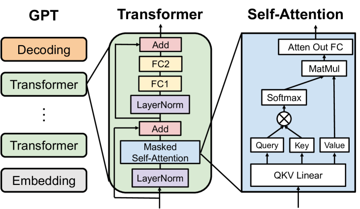
Figure 1. GPT model architecture.

As the popularity of GPT models grows, inference serving systems have evolved to include optimizations specific to the unique architecture and iterative generation pattern of GPT. The major part in GPT’s architecture is a stack of Transformer layers, as shown in Figure 1. In a Transformer layer, the Masked Self-Attention module is the core component that distinguishes it from other architectures like CNNs. For each token in the input, it derives three values, which are query, key, and value. It takes the dot products of query with all the keys of previous tokens to measure the interest of previous tokens from the current token’s point of view. Since GPT is a language model trained to predict the next token, each token should not see information after its location. This is implemented by causal masking in Transformer. It then applies the Softmax to the dot products to get weights and produces the output as a weighted sum of the values according to the weights. At a high level, the attention operator makes each token in the input aware of other tokens regardless of the location distance.

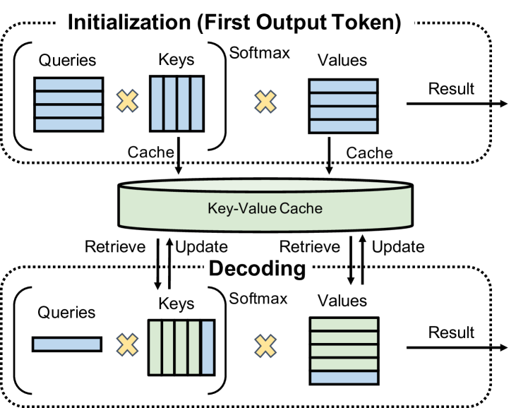
Figure 2. Example usage of KV cache in two phases. The prompt contains four tokens. Blue grids represent newly computed tensors in its iteration, while green grids represent reused tensors from the key-value cache.

During each iteration of GPT inference, for each token, the attention operator requires the keys and values of its preceding tokens. A naive, stateless implementation always recomputes all the keys and values in each iteration. To avoid such recomputation overhead, fairseq (Ott et al., 2019) suggests saving the keys and values in a key-value cache across iterations for reuse. In this way, the inference procedure can be divided into two phases. Figure 2 illustrates the usage of key-value cache in different phases. In the initialization phase, i.e., the first iteration, the prompt is processed to generate the key-value cache for each transformer layer of GPT. In the decoding phase, GPT only needs to compute the query, key, and value of the newly generated token. The key-value cache is utilized and updated to generate tokens step by step. Thus the execution time of iterations in the decoder phase is usually smaller than that of the first iteration. Other system libraries optimized for Transformers such as HuggingFace (Wolf et al., 2020) and FasterTransformer (Corporation, 2019a) also perform the same optimization.

Another optimization is iteration-level scheduling proposed by Orca (Yu et al., 2022). Naive job-level scheduling executes a batch of jobs until all jobs finish. The jobs that finish early cannot return to clients, while newly arrived jobs have to wait until the current batch finishes. Instead, the iteration-level scheduling invokes the execution engine to run only a single iteration on the batch each time, i.e., generate one output token for each job. After each iteration, the finished jobs can leave the batch, and the arrived jobs can join the batch. However, the maximum batch size is limited by the GPU memory capacity, and the low-latency requirement of interactive applications also affects the choice of batch size.

2.3. Opportunities and Challenges

Opportunity: preemptive scheduling. The major limitation of existing inference serving systems for LLMs (Corporation, 2019a; Yu et al., 2022) is that they use simple FCFS scheduling and run-to-completion execution, which has head-of-line blocking and affects JCT. Head-of-line blocking can be addressed by preemptive scheduling. For LLM inference, each job consists of multiple iterations, and each iteration generates one output token. The opportunity is to leverage this autoregressive pattern to enable preemptions at the granularity of each iteration, i.e., preempting one job when it finishes generating an output token for another job. With the capability of preemption, the scheduler can use preemptive scheduling policies to avoid head-of-line blocking and optimize for JCT.

Challenge 1: unknown job size. Shortest Remaining Processing Time (SRPT) (Schrage, 1968) is a well-known preemptive scheduling policy for minimizing average JCT. However, SRPT requires knowledge of the remaining job size. Different from one-shot prediction tasks such as image classification, LLM inference is iterative. While the execution time of one iteration (i.e., generating one output token) can be profiled based on the model architecture and the hardware, the number of iterations (i.e., the output sequence length) is unknown and is also hard to predict, because it is determined by the semantics of the job. Therefore, SRPT cannot be directly applied to LLM inference to minimize average JCT.

Challenge 2: GPU memory overhead. Preemptive scheduling policies introduce extra GPU memory overhead for LLM inference. FCFS with run-to-completion only needs to maintain the key-value cache for the ongoing jobs. In comparison, preemptive scheduling has to keep the key-value cache in the GPU memory for all preempted jobs in the pending state for future token generation. The key-value cache consumes a huge amount of GPU memory. For example, the key-value cache for a single job of GPT-3 175B with input sequence length = 512, requires at least 2.3GB memory (§4.2). The GPU memory capacity limits the key-value cache size and affects the preemptive scheduling policies.

3. FastServe Overview

3.1. Desired Properties

As LLM applications like ChatGPT are becoming popular, delivering high-performance LLM inference is increasingly important. LLMs have their own characteristics that introduce challenges to distributed computation and memory consumption. Our goal is to build an inference serving system for LLMs that meet the following three requirements.

• Low job completion time. We focus on interactive LLM applications. Users expect their jobs to finish quickly. The system should achieve low job completion time for processing inference jobs.

• Efficient GPU memory management. The model parameters and KV cache of LLMs consume tremendous GPU memory. The system should efficiently manage GPU memory to store the model and intermediate state.

• Scalable distributed execution. LLMs require multiple GPUs to perform inference in a distributed manner. The system should provide scalable distributed execution to process LLM inference jobs.

3.2. Overall Architecture

Figure 3. FastServe architecture.

Figure 3 illustrates the architecture of FastServe. Users submit their jobs to the job pool. The skip-join MLFQ scheduler (§4.1) utilizes a profiler to decide the initial priority of newly arrived jobs based on their initiation phase execution time. It adopts iteration-level preemption and favors the least-attained job to address head-of-line blocking issue. Once a job is chosen to be executed, the scheduler sends it to the distributed execution engine (§4.3) which serves the LLM in a GPU cluster and interacts with the distributed key-value cache to retrieve and update the key-value tensors for the corresponding job during runtime. To address the problem of limited GPU memory capacity, the key-value cache manager (§4.2) proactively offloads the key-value tensors of the jobs with low priority to the host memory and dynamically adjusts its offloading strategy based on the burstiness of workload. To scale the system to serve large models like GPT-3 175B, FastServe distributes the model inference across multiple GPUs. Extensions are added to the scheduler and key-value cache to support distributed execution.

4. FastServe Design

In this section, we first describe the skip-join MLFQ scheduler to minimize JCT. Then we present the proactive KV cache management mechanism to handle the GPU memory capacity constraint. At last, we show how to apply these techniques to the distributed setting.

4.1. Skip-Join MLFQ Scheduler

Strawman: naive MLFQ. Because the job size of LLM inference is unknown, SRPT cannot be directly applied. Least-attained service (LAS) is known to approximate SRPT in information-agnostic settings, and MLFQ is a practical approach that realizes discretized LAS to reduce job switching and has been used in many scheduling systems (Hong et al., 2012; Alizadeh et al., 2013; Chowdhury and Stoica, 2015; Bai et al., 2015; Gu et al., 2019). MLFQ has a number of queues, each assigned with a different priority level. An arrival job first enters the highest priority queue and is demoted to the next level queue if it does not finish after a demotion threshold, i.e., quantum, which is a tunable parameter assigned to each queue. Higher priority queues usually have a shorter quantum.

Although MLFQ assumes no prior knowledge of the job size, it is not well suited for LLM serving. Specifically, the first iteration time of a job with a long input sequence length may exceed the quantum of the highest priority queue. When the job gets scheduled, it would use up the quantum in the middle of its first iteration. This creates a dilemma for scheduling. If the scheduler preempts the job, the intermediate activations have to drop and recompute later, which wastes computing resources and time. If the scheduler does not preempt it, then the scheduler violates the design purpose of MLFQ and suffers from head-of-line blocking again.

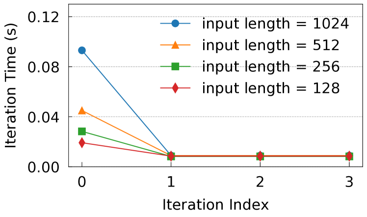
Figure 4. The execution time of the first four iterations (i.e., first four output tokens) with different input sequence length.

Our solution: skip-join MLFQ. Our setting differs from the classic information-agnostic setting in that LLM inference is semi information-agnostic setting. We leverage the characteristics of LLM inference to address the problem of the naive MLFQ. Specifically, although the number of iterations (i.e., the output length) is not known ahead of time, the execution time of each iteration is predictable. The iteration time is determined by a few key parameters such as the hardware, the model, and the input length, and thus can be accurately profiled in advance. Figure 4 shows the iteration time for GPT-3 2.7B on NVIDIA A100 under different input sequence length. We can see that the first iteration time (i.e., the execution time to generate the first output token) is longer than those in the decoding phase within a single job. As the input sequence length increases, the first iteration time grows roughly in a linear manner, while the increase of the iteration time in the decoding phase is negligible. This is due to the key-value cache optimization (§2.2). In the first iteration, all the key-value tensors of the input tokens are computed and cached. While in the following iterations, only the key-value tensors of the newly generated token require computation and others are loaded from the key-value cache, changing the bottleneck from computing to memory bandwidth.

Based on these observations, we design a novel skip-join MLFQ scheduler for LLM inference. Figure 5 highlights the core scheduling operations, and Algorithm 1 shows the pseudo-code. The scheduler uses the basic MLFQ framework with a skip-join feature for new jobs. The quantum of $Q_{1}$ is set to the minimum iteration time and the ratio between $Q_{i}$ and $Q_{i-1}$ is controlled by a parameter quantum ratio. We set it to 2 by default and our experiments (§6.3) show that FastServe’s performance is not sensitive to this quantum setting. After finishing an iteration for the jobs in current processing batch, the scheduler preempts these jobs $J_{pre}$ and invokes the procedure $SkipJoinMLFQScheduler$. This procedure handles newly arrived job $J_{in}$ and constructs a new batch of jobs $J_{out}$ for the execution of next iteration.

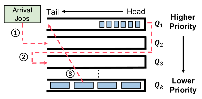
Figure 5. Skip-join MLFQ with starvation prevention.

The scheduler accurately assigns priority to a newly arrived job based on its first iteration time, which is determined by the input sequence length. Specifically, when a job arrives, its priority is set to the highest priority whose quantum is larger than the job’s first iteration time using the $getHighestPriority$ method (lines 7-8). Then the scheduler ❶ skip-joins the job into its corresponding queue rather than the highest priority queue in the naive MLFQ (line 9). For preempted jobs, the scheduler returns the newly generated tokens to the clients immediately, rather than returning the entire response until the completion of the job, which optimizes the user experience (line 12). If the job does not finish and uses up its quantum in the current queue, the scheduler decides the demoted priority of the job based on its current priority and next iteration time by using $getDemotionPriority$ and ❷ demotes it to the corresponding queue (lines 17-20). The skip-join and demotion operations may cause the jobs with long input length or output length to suffer from starvation. To avoid this, the scheduler periodically resets the priority of a job and ❸ promotes it to the highest priority queue $Q_{1}$, if it has been in the waiting state longer than a promotion threshold, $STARVE\_LIMIT$ (lines 22-26). The promoted job will get an extra quantum if its next iteration time is less than the quantum of $Q_{1}$ to ensure its next iteration without preemption. This creates possibility of head-of-line blocking, so the system administrator of FastServe can tune $STARVE\_LIMIT$ to make a tradeoff between performance and starvation. At last, the scheduler selects a set of jobs with the highest priority without exceeding the maximum batch size, which constrained by the GPU memory capacity (lines 28-31). By utilizing the characteristics of LLM inference, the skip-join MLFQ scheduler can adjust the job priority more accurately and reduce demotions. Thus it achieves better approximation to SRPT than the naive MLFQ.

Algorithm 1 Skip-Join Multi-Level Feedback Queue Scheduler

1:Input: Queues $Q_{1},Q_{2},...,Q_{k}$, newly arrived jobs $J_{in}$, preempted jobs $J_{pre}$, and profiling information $P$

2:Output: Jobs to be executed $J_{out}$

3:procedure SkipJoinMLFQScheduler

4:    Initialization: $J_{out}\leftarrow\emptyset$.

5:    // Process newly arrival jobs.

6:    for $job\in J_{in}$ do

7:         $nextIterTime\leftarrow P.getNextIterTime(job)$

8:         $p_{job}\leftarrow getHighestPriority(nextIterTime)$

9:         $Q_{p_{job}}.push(job)$     

10:    // Process preempted jobs.

11:    for $job\in J_{pre}$ do

12:         $job.outputNewGeneratedToken()$

13:         $p_{job}\leftarrow job.getCurrentPriority()$

14:         if $job.isFinished()$ then

15:             $Q_{p_{job}}.pop(job)$

16:             continue          

17:         if $job.needDemotion()$ then

18:             $nextIterTime^{\prime}\leftarrow P.getNextIterTime(job)$

19:             $p_{job}^{\prime}\leftarrow getDemotionPriority(p_{job},nextIterTime^{\prime})$

20:             $r.demoteTo(Q_{p_{job}^{\prime}})$              

21:    // Promote starved jobs.

22:    for $q\in\{Q_{2},Q_{3},...,Q_{k}\}$ do

23:         for $job\in q$ do

24:             if $job.needPromotion()$ then

25:                 $job.promoteTo(Q_{1})$

26:                 $job.resetStarveTimer()$                           

27:    // Schedule jobs to be executed.

28:    for $q\in\{Q_{1},Q_{2},...,Q_{k}\}$ do

29:         for $job\in q$ do

30:             if $job.isReady()$ and $|J_{out}|<MaxBatchSize$ then

31:                 $J_{out}.push(job)$                           

Example. Figure 6 shows an example to illustrate our scheduler and compares it against the alternatives. Three jobs arrive at time $0$ in the order of $J_{1},J_{2},J_{3}$, where their first iteration times are 5, 1, and 2, respectively, and their output lengths are all equal to 2. We assume the iteration time in the decoding phase is 1 for simplicity. Skip-join MLFQ and Naive MLFQ both have four priority queues with quantum 1, 2, 4, and 8. For Naive MLFQ, it does interrupt the iteration if a job uses up its quantum during execution. The average JCT of FCFS, naive MLFQ, skip-join MLFQ, and SRPT are 8.33, 10, 6.67, and 6, respectively. In general, the algorithms with more information perform better than those with less information in minimizing JCT. Without skip-join, naive MLFQ may degenerate to round-robin and be worse than FCFS in some cases.

4.2. Proactive Key-Value Cache Management

The skip-join MLFQ scheduler provides iteration-level preemption to approximate SRPT without knowing the exact job size. However, preemption also increases the number of ongoing jobs in the system, which introduces extra GPU memory overhead. Formally, for a particular LLM inference serving job, denote the input sequence length by $s$, the output sequence length by $t$, the hidden dimension of the transformer by $h$, and the number of transformer layers by $l$. If the model weights and all computations are in FP16, the total number of bytes to store the key-value cache for this single job is $4\times lh(s+t)$. Take GPT-3 175B as an example $(l=96,h=12288)$. Given an input sequence length $s=512$ and a minimum output sequence length $t=1$, the GPU memory overhead for a single job is as high as $2.3$GB. As the generation continues, its output sequence length $t$ will increase, which further increases the GPU memory overhead.

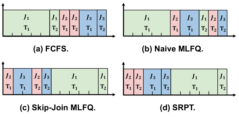
Figure 6. Execution timeline of three jobs with different scheduling algorithms. The job index $J_{i}$ and generated token index $T_{i}$ are marked in each iteration block.

The schedulers using the run-to-completion policy can tolerate this memory overhead because the maximum number of ongoing jobs would not exceed the size of the current processing batch. Figure 7 shows the key-value cache memory consumption of FCFS and skip-join MLFQ for GPT-3 2.7B model under a synthetic workload. Although we choose a relatively small model and limit the maximum output length to 20, the peak KV cache memory overhead for skip-join MLFQ can be $7\times$ larger than that of FCFS. In a more realistic scenario where the model size scales to 175B and the output length can be more than a thousand, the memory overhead for skip-join MLFQ can easily exceed the memory capacity of NVIDIA’s newest Hopper 80 GB GPUs.

Strawman solution 1: defer newly arrived jobs. A naive solution is to simply defer the execution of newly arrived jobs when the GPU memory is not sufficient to hold additional key-value tensors and keep scheduling current jobs until they finish. Although new jobs often have higher priority, they have to be blocked to wait for free memory space. Under extreme GPU memory-constrained settings, this solution would degenerate MLFQ to FCFS, which again suffers from head-of-line blocking.

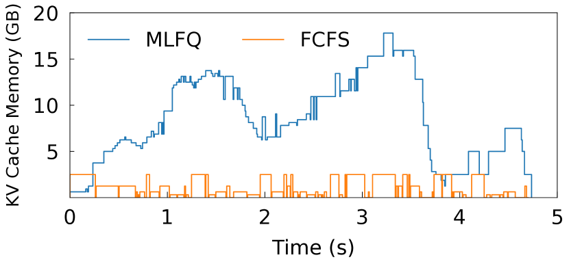
Figure 7. The key-value cache memory consumption for GPT-3 2.7B under different schedulers. The workload follows a Gamma Process with rate=64 and CV=4. The maximum output length is set to 20 to avoid GPU out of memory.

Strawman solution 2: kill low-priority jobs. Another straightforward solution is to kill some low-priority jobs and free their key-value cache to make room for newly arrived high-priority jobs. This solution has two problems. First, the killed jobs lose their generation state and need to rerun the initiation phase to generate their key-value cache, which wastes computation resources and time. Second, it may cause deadlocks. When the high-priority jobs keep arriving, ongoing jobs with lower priority would be killed. With the starvation avoidance mechanism enabled, the killed jobs may be promoted to the highest-priority queue after $STARVE\_LIMIT$. In this case, the promoted job may again kill the currently executing job that kills it in the previous round, which leads to a deadlock. This brings extra complexity to set $STARVE\_LIMIT$. A large value causes starvation, while a small value may cause deadlocks.

Our solution: proactive key-value cache swapping. From the two strawman solutions, we can see a dilemma that MLFQ requires more GPU memory for better performance, while the limited GPU memory restricts the potential of the scheduling based on MLFQ. To solve this problem, our key observation is that the key-value tensors only need to be reserved in the GPU memory when its corresponding job gets scheduled. Based on this observation, FastServe can offload inactive key-value tensors of jobs to the host memory and upload necessary key-value tensors back to the GPU memory when they are needed. The challenge is that the overhead of offloading and uploading is not negligible compared to the token generation time. When deploying GPT-3 175B on NVIDIA A100 GPUs, the key-value tensors of a job can occupy 2.3 GB memory. The token generation time in decoding phase is about 250ms, while the time to transfer the key-value tensors between host memory and GPU memory with PCIe 4.0$\times$16 full bandwidth is about 36ms.

FastServe uses proactive offloading and uploading to minimize the swapping overhead. Instead of reactively offloading jobs when the key-value cache is full, FastServe keeps some idle key-value cache slot for newly arrived jobs. When a new job arrives, it can get a key-value cache slot immediately without incurring the overhead of offloading a preempted job. Rather than reactively uploading the key-value tensors for the executed job, when the key-value cache space on the GPU is sufficient, FastServe proactively uploads the key-value tensors of the jobs that will be used in the near future so that the token generation can be overlapped with the data transmission.

The number of idle key-value cache is the maximum of a tunable parameter set by the system administrator, $K$, and the value provided by a burst predictor. The tunable parameter $K$ ensures that at least $K$ newly arrived job will not be blocked by the offloading. The burst predictor is a heuristic that predicts the number of jobs that will arrive in the near future. When a burst of jobs arrives, the predictor leaves more idle key-value cache slots in advance. We use the number of jobs in the top $K^{\prime}$ priority queues as the prediction, where $K^{\prime}$ is also a tunable parameter. Empirically, we find that the performance is not sensitive to the choices of $K$ and $K^{\prime}$.

Job swapping order. To mitigate the impact of job swapping, the decision on the order of offloading and uploading is made based on a metric, the estimated next scheduled time (ENST). The ENST is the time when the job will be scheduled to execute next time. The job with the largest ENST will be offloaded first, and the job with the smallest ENST will be uploaded first. In general, the lower priority a job has, the later it will be scheduled to execute. However, due to the starvation prevention mechanism, a job with a lower priority may be promoted to a higher priority queue. In this case, a job with a low priority may also be executed first.

To handle this case, for job $i$, FastServe considers the time to promote this job and the sum of executed time of all jobs with higher priorities before executing $i$. Formally, let the time to promote as $T_{promote}(i)$. As for the sum of executed time of all jobs with higher priorities before executing $i$, we assume those jobs do not finish earlier before being demoted to the priority queue of $i$. In this case, the execution time of job $j$ with a higher priority can be calculated as follows:

$$T_{execute}(i,j)=\sum_{i.priority<k\leq j.priority}quantum(k)$$

where $i.priority$ is the priority of job $i$, and $quantum(k)$ is the quantum of the priority queue with priority $k$. Based on this, the sum of executed time of all jobs with higher priorities than job $i$ is defined as:

$$T_{execute}(i)=\sum_{i.priority<j.priority}T_{execute}(i,j)$$

At last, taking both the promotion for starvation prevention and the execution of higher priority jobs into consideration, the ENST of job $i$ is calculated as:

$$ENST(i)=\min(T_{promote}(i),T_{execute}(i))$$

This ENST definition estimates how long job $i$ will be scheduled to execute. Therefore, using this metric to decide the order of offloading and uploading makes the key-value tensors of active jobs more likely on the GPU memory, and those of inactive jobs more likely on the host memory. This hides the swapping overhead as much as possible.

4.3. Support for Distributed LLM Serving

Previous research shows that the capability of LLMs empirically conforms to the scaling law in terms of the number of model parameters (Kaplan et al., 2020). The more parameters an LLM has, the more powerful an LLM can be. However, the memory usage of an LLM is also proportional to the number of parameters. For example, GPT-3 175B when stored in half-precision, occupies 350GB GPU memory to just hold the weights and more for the intermediate state during runtime. Therefore, LLM often needs to be split into multiple pieces and served in a distributed manner with multiple GPUs.

Tensor parallelism (Shoeybi et al., 2020; Narayanan et al., 2021) and pipeline parallelism (Huang et al., 2019; Narayanan et al., 2019) are two most widely-used techniques for distributed execution of deep learning models. FastServe supports the hybrid of these two parallel techniques for serving LLMs. An LLM is composed of a series of operators over multi-dimensional tensors. Tensor parallelism splits each operator across multiple devices, with each device executing a portion of the computation in parallel. Additional communication overhead is required to split the input and collect the output from participating GPUs. Tensor parallelism expands the computation and memory available to a single job, thus reduces the execution time for each iteration.

Pipeline parallelism splits the operators of an LLM computation graph into multiple stages and executes them on different devices in a pipeline fashion. During inference, each stage computes part of the entire computation graph and transmits the intermediate results to the next stage in parallel. Pipeline parallelism requires less communication overhead compared to tensor parallelism and also allows the LLM to exceed the memory limitation of a single GPU. Since multiple processing batches are under processing simultaneously in different stages, FastServe needs to handle multiple batches in the distributed engine at the same time.

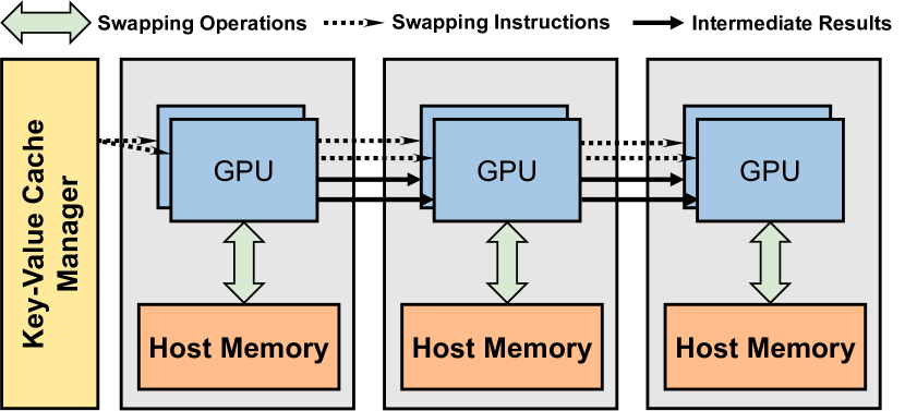
Figure 8. Overlapping key-value cache offloading with intermediate result transmission to reduce offloading overhead.

Job scheduling in distributed serving. In the traditional MLFQ setting, if no new job arrives, the scheduler would schedule the job with the highest priority and executes it until it finishes or is demoted. However, when using pipeline parallelism, the scheduler schedules at the granularity of the stage. When a job finishes the first stage and sends the intermediate result to the next stage, the scheduler needs to decide on the next job to execute. In this case, the scheduler cannot follow the traditional MLFQ that keeps scheduling the same job until demotion, because the job is still running. To preserve the semantics of MLFQ, FastServe still keeps the running job in the priority queue, and each time selects the highest priority job in the pending state to execute. Therefore, the early job in a queue can finish the quantum more quickly.

Key-value cache management in distributed serving. Because the key-value cache occupies a large fraction of GPU memory, the key-value cache of FastServe is also partitioned across multiple GPUs in distributed serving. In LLM inference, each key-value tensor is used by the same stage of the LLM. Therefore, FastServe partitions key-value tensors as tensor parallelism requires, and assigns each key-value tensor to the corresponding GPU so that all computation on a GPU only needs local key-value tensors.

The proactive key-value cache swapping mechanism of FastServe is also distributed. Because different stages of the LLM process different jobs at the same time, each stage may offload or upload different key-value tensors independently. To reduce redundant control, before processing the intermediate result sent from the previous stage, the current stage does the same offloading or uploading action as the previous stage does. The intermediate result transmission and key-value cache swapping occur in parallel, so the overhead of key-value cache swapping is further reduced. As shown in Figure 8, when the intermediate result is sent to the next stage, the next stage receives the swapping instructions and can swap the key-value cache at the same time if needed. The key-value cache swapping mechanism only needs to decide the offloading or uploading of the first stage. When using tensor parallelism splitting the first stage into multiple chunks, a centralized key-value cache swapping manager instructs all chunks in the first stage to offload or upload the key-value tensors owned by the same job.

5. Implementation

We implement FastServe with 10,000 lines of code in Python and C++. The distributed execution engine is based on NVIDIA FasterTransformer(Corporation, 2019a) which is a high-performance transformer library with custom CUDA kernel implementation. We modify it to support iteration-level scheduling and interact with the key-value cache manager. We also add extensions to its pipeline parallelism because its original job-level scheduling implementation does not allow injecting another batch before the finish of the currently running batch. It can only split a batch of jobs into multiple microbatches (Huang et al., 2019) and pipelines the executions of different pipeline stages across the microbatches. This loses the chance to pipeline execution between job batches, and smaller microbatches reduce device utilization. In our implementation, the execution engine can receive a new batch of jobs as soon as the first pipeline stage finishes execution, which means every partition of the model processes one of the batches without being idle.

We implement the key-value cache manager with MPI (Gabriel et al., 2004) in a distributed manner, because the key-value tensors are produced and consumed on different GPUs. The distributed design makes it possible to save and retrieve the key-value tensors on the corresponding GPUs, which minimizes the data transfer overhead. We also use MPI to pass messages to synchronize the offloading procedure across the GPUs and utilize multiple CUDA streams to overlap the computation with proactive swapping.

6. Evaluation

In this section, we first use end-to-end experiments to demonstrate the overall performance improvements of FastServe over state-of-the-art LLM serving systems on GPT-175B(Brown et al., 2020). Next, we deep dive into FastServe to evaluate its design choices and show the effectiveness of each component in FastServe under a variety of settings. Last, we analyze the scalability of FastServe under different numbers of GPUs.

6.1. Methodology

Testbed. The end-to-end (§6.2) and scalability (§6.4) experiments use two AWS EC2 p4d.24xlarge instances. Each instance is configured with eight NVIDIA A100 40GB GPUs connected over NVLink, 1152 GB host memory, and PCIe 4.0$\times$16. Due to the limited budget, the experiments for design choices (§6.3) use one NVIDIA A100 40GB GPU in our own testbed to validate the effectiveness of each component.

LLM models. We choose the representative LLM family, GPT (Brown et al., 2020), for evaluation, which is widely used in both academics and industry. In LLM serving, the large model weights are usually pre-trained and then fine-tuned into different versions to serve different tasks. We select several widely used model sizes (Brown et al., 2020) for different experiments. Table 1 lists the detailed model sizes and model configurations. We use FP16 precision for all experiments in our evaluation.

Workloads. Similar to prior work on LLM serving (Yu et al., 2022), we synthesize a trace of jobs to evaluate the performance of FastServe, since there is no publicly-available job trace for LLM inference. The job size is generated by sampling a random input and output length from a Zipf distribution which is broadly adopted in many open-source big data benchmarks (Cooper et al., 2010; Chen et al., 2012; Gao et al., 2013; Watson et al., 2017). The Zipf distribution is parameterized by one parameter, $\theta$, which controls the skewness of the distribution. The larger $\theta$ is, the more skewed the workload is, with more long-tail jobs appearing in the workload. We generate the arrival time for each job following a Gamma process parameterized by arrival rate and coefficient of variation (CV). By scaling the rate and CV, we can control the rate and burstiness of the workload, respectively.

Metrics. Since the user-perceived latency is a critical measurement for interactive applications like ChatGPT, which FastServe targets at, we use job completion time (JCT) as the major evaluation metric. Due to limited space, we show average JCT for most experiments, and report both average and tail JCT in the scalability experiments.

Baselines. We compare FastServe with two baselines.

• FasterTransformer (Corporation, 2019a): It is an open-source production-grade distributed inference engine from NVIDIA, which optimizes for large transformer-based language models and is widely used in industry. It supports both tensor parallelism and pipeline parallelism for distributed execution. However, it adopts request-level scheduling and thus does not support pipelining across different jobs as discussed in section §5.

• Orca (Yu et al., 2022): It is the state-of-the-art LLM serving system that supports iteration-level scheduling and inter-job pipeline parallelism to reduce pipeline bubbles. However, it uses a simple FCFS scheduler with run-to-completion execution, which suffers from head-of-line blocking. Since Orca is not open-sourced, we implement Orca on top of FasterTransformer for a fair comparison.

Model	Size	# of Layers	# of Heads	Hidden Size
GPT-3 2.7B	5.4GB	32	32	2560
GPT-3 66B	132GB	64	72	9216
GPT-3 175B	350GB	96	96	12288

Table 1. Model configurations.

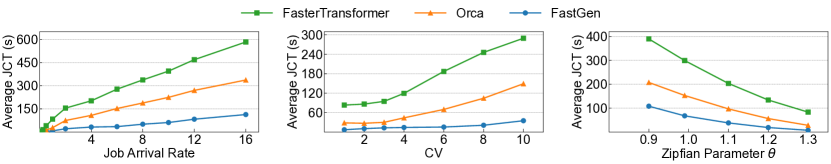
(a) Average JCT vs. load.                    (b) Average JCT vs. burstiness.             (c) Average JCT vs. skewness.

Figure 9. End-to-end performance when serving GPT-3 175B with 16 NVIDIA A100 40GB GPUs.

6.2. Overall Performance

In this subsection, we compare the performance of FastServe to the two baseline systems under a variety of workload settings on GPT-175B. We use two AWS p4d.24xlarge instances with 16 NVIDIA A100 40GB GPUs in total. We use a mix of tensor parallelism and pipeline parallelism. Specifically, the model is partitioned with tensor parallelism in each instance as the eight A100 GPUs in each instance are connected over NVLink with high bandwidth. The two instances execute the jobs through pipeline parallelism which is connected over Ethernet. FastServe significantly outperforms the two baseline systems with its skip-join MLFQ scheduler and proactive key-value cache management, which we summarize as follows.

Average JCT vs. load. Figure 9(a) varies the job arrival rate while keeping other parameters (e.g., CV and Zipf parameter) the same. FastServe outperforms Orca by 1$\times$–4.3$\times$ and FasterTransformer by 1.9$\times$–11.4$\times$. When the rate is low ($\leq$ 0.5), FastServe has the same performance as Orca but outperforms FasterTransformer by around 2$\times$. This is because MLFQ deteriorates into FCFS at a low job arrival rate. FasterTransformer does not support inter-job pipelining which leads to only 50% GPU utilization due to the bubbles in the pipeline. As the rate grows, the head-of-line blocking problem of FCFS becomes more severe. FastServe consistently outperforms Orca by at least 3$\times$ and FasterTransformer by at least 5$\times$ when the rate is greater than 0.5. FastServe is able to effectively reduce the head-of-line blocking by prioritizing the short jobs with skip-join MLFQ.

Average JCT vs. burstiness. Figure 9(b) varies the CV, which controls the burstiness of job arrivals while keeping other parameters (e.g., rate and Zipfian parameter) the same. FastServe outperforms Orca by 2.3$\times$–5.1$\times$ and FasterTransformer by 7.4$\times$–12.2$\times$. When the CV is low, the jobs arrive reposefully. As a result, the performance gap between FastServe and the two baselines is small. However, when the CV is high, the jobs arrive in a bursty manner, which exacerbates the head-of-line blocking problem. The bursty workload also introduces significant pressure on key-value cache management. With the proactive swapping mechanism, FastServe significantly outperforms the two baselines under high CV.

Average JCT vs. skewness. Figure 9(c) varies the Zipfian parameter $\theta$, which controls the skewness of the input and output sequence lengths (i.e., the skewness of job size) while keeping other parameters (e.g., rate and CV) the same. FastServe outperforms Orca by 1.9$\times$–3.9$\times$ and FasterTransformer by 3.6$\times$-10.6$\times$. When $\theta$ is small, the input and output lengths of the jobs are more balanced. As a result, the performance gap between FastServe and the two baselines is small. When $\theta$ becomes large, the input and output lengths of the jobs are more skewed. Thus, FastServe benefits more from the skip-join MLFQ scheduler to tame the head-of-line blocking problem. It is worth noting that the absolute value of JCT increases as $\theta$ decreases. This is because we bound the maximum input and output lengths. As a result, the workloads with smaller $\theta$ (i.e., balanced job lengths) have more tokens to process.

6.3. Benefits of Design Choices

In this subsection, we study the effectiveness of FastServe’s main techniques: skip-join MLFQ scheduler and proactive key-value cache management. Due to a limited budget, we use one A100 GPU to run GPT-3 2.7B in the experiments.

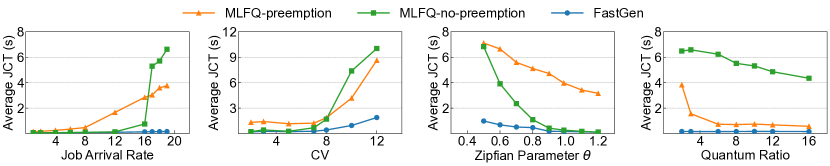
(a) Ave. JCT vs. load.           (b) Ave. JCT vs. burstiness.       (c) Ave. JCT vs. skewness.     (d) Ave. JCT vs. quantum ratio.

Figure 10. Benefits of the skip-join MLFQ scheduler in FastServe.

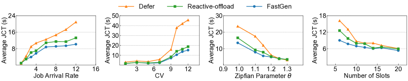
(a) Ave. JCT vs. load.           (b) Ave. JCT vs. burstiness.       (c) Ave. JCT vs. skewness.         (d) Ave. JCT vs. cache size.

Figure 11. Benefits of the proactive key-value cache management mechanism in FastServe.

Benefits of skip-join MLFQ. To show the benefits of the skip-join MLFQ scheduler, we compare it with two baseline MLFQ schedulers.

• MLFQ with preemption (MLFQ-preemption): It is agnostic to the input length, and puts a newly arrived job to the queue with the highest priority. If the corresponding quantum is not enough to execute an iteration, it preempts (i.e., kills) the current iteration and demotes the job.

• MLFQ without preemption (MLFQ-no-preemption): It is also agnostic to the input length. However, if the corresponding quantum is not enough, it continues to execute the halfway iteration and then demotes the job. It degenerates to round-robin scheduling if the quantum is always insufficient.

Similar to previous experiments, we vary the rate, CV, and Zipfian parameter of the workload. In addition, to evaluate the sensitivity of MLFQ to the quantum settings, we vary the quantum ratio (§4.1) to see the impact on performance. The results are summarized as follows.

As Figure 10(a) shows, when the rate is low, there is little or even no queueing. Thus, all three schedulers degenerate to FCFS and have similar performance. As the rate grows, MLFQ-preemption suffers from re-execution overhead of halfway iterations since the quantum of the high-priority queues may be not enough to execute the first iteration of some jobs. As for MLFQ-no-preemption, its average JCT increases dramatically when the rate is slightly over 16 since some large jobs in the highest priority queue block too many jobs from execution. As a result, FastServe outperforms the two baseline MLFQ schedulers by up to 24$\times$ through its skip-join technique. When varying CV, the performance gap is similar. As shown by Figure 10(b), FastServe outperforms the two baselines by up to 7.8$\times$.

As demonstrated by Figure 10(c), FastServe consistently outperforms MLFQ-preemption and MLFQ-no-preemption by up to 32$\times$, due to the re-execution overhead of MLFQ-preemption and the head-of-line blocking problem of MLFQ-no-preemption. The performance gap between FastServe and MLFQ-no-preemption becomes larger as the Zipfian parameter $\theta$ decreases. This is because a small $\theta$ leads to a more balanced distribution of input lengths for each job, making more jobs’ first iteration time surpass the quantum of the first few high-priority queues. As a result, MLFQ-no-preemption degenerates to round-robin, so FastServe significantly outperforms MLFQ-no-preemption under such conditions.

In Figure 10(d), it is worth noting that increasing the quantum ratio has little impact on the performance of FastServe, but it reduces the JCT of the two baseline MLFQ schedulers. This demonstrates that FastServe is not sensitive to the quantum settings, making the life of the system administrator much easier. For MLFQ-preemption, enlarging the quantum of each priority queue mitigates the re-execution overhead of preempted inference jobs. For MLFQ-no-preemption, a small quantum makes each job get processed in a round-robin fashion. The problem is mitigated as the quantum increases, so MLFQ-no-preemption performs better. Also, we can see a performance gap between the two baselines even when the quantum ratio grows to 16, indicating that compared to re-execution overhead, head-of-line blocking is a more severe performance issue. With skip-join MLFQ, FastServe is able to address the problems of the two baseline MLFQ schedulers and outperforms both of them. Overall, FastServe outperforms the two baseline MLFQ schedulers by 3.6$\times$–41$\times$.

Benefits of proactive key-value cache management. To show the benefits of the proactive key-value cache management mechanism, we compare it with two baseline key-value cache management mechanisms.

• Defer: It defers an upcoming job if the key-value cache slots are all used. The job waits until a key-value cache slot is available.

• Reactive-offload: When the key-value cache is full and a scheduled job is unable to get an empty slot, it reactively picks a job in the cache and offloads its state to the host memory. The cache replacement policy (i.e., picking which job to offload) is the same as FastServe.

Similar to previous experiments, we vary the rate, CV, and Zipfian parameter of the workload. In addition, we adjust the number of slots of the GPU key-value cache as an additional factor to evaluate the sensitivity of proactive key-value cache management to the cache size.

As shown in Figure 11(a), when the job arrival rate is low, the performance gap between FastServe and the two baselines is small, since the peak memory usage is low and the key-value cache is sufficient for all three solutions. As the job arrival rate grows, the peak memory usage exceeds the GPU memory capacity, making FastServe significantly outperform Defer by up to 2.3$\times$. For Reactive-offload, the high job arrival rate leads to more jobs that require key-value cache slots to arrive at the same time, but all need to wait for extra data transmission time. Therefore, FastServe is able to achieve 1.6$\times$ better performance than Reactive-offload. As for the impact of burstiness in Figure 11(b), FastServe also outperforms Defer and Reactive-offload by up to 3.5$\times$ and 1.4$\times$, respectively, due to the overlapping between proactive swapping and computation. For the impact of skewness in Figure 11(c), the performance gap becomes larger as the Zipfian parameter $\theta$ reduces. This is because the average job size becomes larger, due to the bounded maximum length and less skewness. Consequently, the peak memory usage increases, leading to more improvements of FastServe. As for Figure 11(d), when the number of key-value cache slots is small, the peak memory usage easily exceeds the key-value cache size, which requires more careful cache management. With overlapping the proactive swapping and computation, FastServe is able to outperform Defer and Reactive-offload by up to 1.8$\times$. Note that when serving 175B-scale models, the cache size is greatly limited by the GPU memory capacity, making proactive swapping management a necessity.

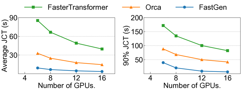
(a) Average JCT.                      (b) Tail JCT.

Figure 12. Scalability experiments under different number of NVIDIA A100 40GB GPUs when serving GPT-3 66B.

6.4. Scalability

In this subsection, we evaluate the scalability of FastServe for serving GPT-3 66B model. We vary the number of GPUs while fixing other parameters in the experiments to compare FastServe with FasterTransformer and Orca. The model is divided into two pipeline stages and tensor parallelism is adjusted accordingly based on the number of GPUs. Note that we do not use GPT-3 175B, because it needs at least 9 NVIDIA A100 40GB GPUs to just hold its weights and consumes more memory for the intermediate state during inference serving. GPT-3 66B can be served with only 6 NVIDIA A100 40GB GPUs, allowing us to vary the number of GPUs from 6 to 16 to evaluate the scalability. We report both average JCT and tail JCT (90% JCT) in the results. As shown in Figure 12, both average JCT and tail JCT decrease when more GPUs are used to serve inference jobs, as more computing resources speed up the execution time of each job with tensor parallelism. With careful integration with distributed execution, FastServe supports iter-job pipeline parallelism in its scheduler, and benefits from memory locality through its distributed key-value cache management. The results show that FastServe achieves 3.5$\times$–4$\times$ and 9.2$\times$–11.1$\times$ improvement on average JCT than Orca and FasterTransformer, respectively. As for 90% tail JCT, FastServe outperforms them by 2.2$\times$–6.4$\times$ and 4.3$\times$–12.5$\times$, respectively.

7. Related Work

Preemptive scheduling. Many solutions for job scheduling in datacenters use preemptive scheduling. PDQ (Hong et al., 2012), pFabric (Alizadeh et al., 2013), Varys (Chowdhury et al., 2014), and PIAS (Bai et al., 2015) use preemptive flow scheduling to minimize flow completion time. Shinjuku (Kaffes et al., 2019b), Shenango(Ousterhout et al., 2019), and Caladan (Fried et al., 2020) focus on latency-sensitive datacenter workloads, which use fine-grained preemption and resource reallocation to optimize for microsecond-scale tail latency. As for DL workloads, Tiresias (Gu et al., 2019) uses MLFQ to optimize JCT for distributed DL training jobs. Pipeswitch(Bai et al., 2020) and REEF(Han et al., 2022) provide efficient GPU preemption to run both latency-critical and best-effort DL tasks to achieve both real-time and work conserving on GPU. By contrast, FastServe targets a new scenario, LLM inference serving, and is semi information-agnostic.

Inference serving. TensorFlow Serving (Olston et al., 2017) and Triton Inference Server (Corporation, 2019b) are production-grade inference serving systems, which are widely used in industry. They serve as an abstraction above the execution engines and lack model-specific optimizations. Clipper (Crankshaw et al., 2017), Clockwork (Gujarati et al., 2020), and Shepherd (Zhang et al., 2023) focus on serving relatively small models like ResNet in a cluster and support latency-aware provision to maximize the overall goodput. INFaaS (Romero et al., 2021) proposes a model-less serving paradigm to automate the model selection, deployment, and serving process. There are also serving systems that incorporate domain-specific knowledge, such as Nexus (Shen et al., 2019) which targets DNN-based video analysis, and Inferline (Crankshaw et al., 2020) which optimizes the serving pipeline that consists of multiple models. Recently, several serving systems are proposed to optimize Transformer-based LLMs (Fang et al., 2021; Li et al., 2023, 2023; Yu et al., 2022). Orca (Yu et al., 2022) is the state-of-the-art solution that considers the autoregressive generation pattern of LLMs. However, its FCFS policy suffers from head-of-line blocking which we address in this paper.

Memory management for LLMs. Due to high memory usage for LLMs, many techniques have been proposed to reduce memory overhead. Some work (Bai et al., 2021; Wang et al., 2023) targets training, which is orthogonal to the serving scenario. Quantization (Li et al., 2020; Xiao et al., 2022; Frantar et al., 2022; Dettmers et al., 2022) compresses the model weights into 8-bit or even 4-bit integers after training, which can greatly reduce the memory footprint during inference. Similarly, SparTA (Zheng et al., 2022) is an end-to-end model sparsity framework to explore better sparse models. However, these approaches can decrease the performance of the original model. Petals (Borzunov et al., 2022) runs the inference of LLMs in a collaborative fashion to amortize the cost via decentralization. Its performance is influenced due to network latency. Other works (Aminabadi et al., 2022; HuggingFace, 2022; Sheng et al., 2023) use offloading to utilize host memory and disks. FlexGen (Sheng et al., 2023) pushes this idea to support 175B-scale model with a single GPU. However, they all use a run-to-completion policy. To hide the data transmission time with computation, they target offline throughput-oriented applications which process a big batch at a time and are not suitable for interactive applications like ChatGPT. FastServe exploits preemption at the granularity of iteration to optimize for JCT.

8. Conclusion

We present FastServe, a distributed inference serving system for LLMs. We exploit the autoregressive pattern of LLM inference to enable iteration-level preemption and design a novel skip-join MLFQ scheduler to address head-of-line blocking. We propose a proactive key-value cache management mechanism to handle the memory overhead of the key-value cache and hide the data transmission latency with computing. Based on these techniques, we build a prototype of FastServe. Experiments show that FastServe improves the average JCT and tail JCT by up to 5.1$\times$ and 6.4$\times$ respectively, compared to the state-of-the-art solution Orca.

References

- (1)
- cha (2022) 2022. Introducing ChatGPT. https://openai.com/blog/chatgpt. (2022).
- bar (2023) 2023. Bard, an experiment by Google. https://bard.google.com/. (2023).
- cha (2023) 2023. ChatGPT sets record for fastest-growing user base. https://www.reuters.com/technology/chatgpt-sets-record-fastest-growing-user-base-analyst-note-2023-02-01/. (2023).
- dol (2023) 2023. Hello Dolly: Democratizing the magic of ChatGPT with open models. https://www.databricks.com/blog/2023/03/24/hello-dolly-democratizing-magic-chatgpt-open-models.html. (2023).
- new (2023) 2023. Reinventing search with a new AI-powered Bing and Edge, your copilot for the web. https://news.microsoft.com/the-new-Bing/. (2023).
- Alizadeh et al. (2013) Mohammad Alizadeh, Shuang Yang, Milad Sharif, Sachin Katti, Nick McKeown, Balaji Prabhakar, and Scott Shenker. 2013. pfabric: Minimal near-optimal datacenter transport. SIGCOMM CCR (2013).
- Aminabadi et al. (2022) Reza Yazdani Aminabadi, Samyam Rajbhandari, Minjia Zhang, Ammar Ahmad Awan, Cheng Li, Du Li, Elton Zheng, Jeff Rasley, Shaden Smith, Olatunji Ruwase, et al. 2022. Deepspeed inference: Enabling efficient inference of transformer models at unprecedented scale. arXiv (2022).
- Bai et al. (2015) Wei Bai, Li Chen, Kai Chen, Dongsu Han, Chen Tian, and Hao Wang. 2015. Information-agnostic flow scheduling for commodity data centers. In USENIX OSDI.
- Bai et al. (2021) Youhui Bai, Cheng Li, Quan Zhou, Jun Yi, Ping Gong, Feng Yan, Ruichuan Chen, and Yinlong Xu. 2021. Gradient Compression Supercharged High-Performance Data Parallel DNN Training. In ACM SOSP.
- Bai et al. (2020) Zhihao Bai, Zhen Zhang, Yibo Zhu, and Xin Jin. 2020. Pipeswitch: Fast pipelined context switching for deep learning applications. In USENIX OSDI.
- Borzunov et al. (2022) Alexander Borzunov, Dmitry Baranchuk, Tim Dettmers, Max Ryabinin, Younes Belkada, Artem Chumachenko, Pavel Samygin, and Colin Raffel. 2022. Petals: Collaborative inference and fine-tuning of large models. arXiv (2022).
- Brown et al. (2020) Tom B. Brown, Benjamin Mann, Nick Ryder, Melanie Subbiah, Jared Kaplan, Prafulla Dhariwal, Arvind Neelakantan, Pranav Shyam, Girish Sastry, Amanda Askell, Sandhini Agarwal, Ariel Herbert-Voss, Gretchen Krueger, Tom Henighan, Rewon Child, Aditya Ramesh, Daniel M. Ziegler, Jeffrey Wu, Clemens Winter, Christopher Hesse, Mark Chen, Eric Sigler, Mateusz Litwin, Scott Gray, Benjamin Chess, Jack Clark, Christopher Berner, Sam McCandlish, Alec Radford, Ilya Sutskever, and Dario Amodei. 2020. Language Models are Few-Shot Learners. (2020).
- Chen et al. (2012) Yanpei Chen, Sara Alspaugh, and Randy Katz. 2012. Interactive analytical processing in big data systems: A cross-industry study of mapreduce workloads. arXiv (2012).
- Chiang et al. (2023) Wei-Lin Chiang, Zhuohan Li, Zi Lin, Ying Sheng, Zhanghao Wu, Hao Zhang, Lianmin Zheng, Siyuan Zhuang, Yonghao Zhuang, Joseph E. Gonzalez, Ion Stoica, and Eric P. Xing. 2023. Vicuna: An Open-Source Chatbot Impressing GPT-4 with 90%* ChatGPT Quality. (2023). https://vicuna.lmsys.org
- Chowdhury and Stoica (2015) Mosharaf Chowdhury and Ion Stoica. 2015. Efficient coflow scheduling without prior knowledge. SIGCOMM CCR (2015).
- Chowdhury et al. (2014) Mosharaf Chowdhury, Yuan Zhong, and Ion Stoica. 2014. Efficient coflow scheduling with varys. In ACM SIGCOMM.
- Cooper et al. (2010) Brian F Cooper, Adam Silberstein, Erwin Tam, Raghu Ramakrishnan, and Russell Sears. 2010. Benchmarking cloud serving systems with YCSB. In ACM Symposium on Cloud Computing.
- Corporation (2019a) NVIDIA Corporation. 2019a. FasterTransformer. (2019). https://github.com/NVIDIA/FasterTransformer
- Corporation (2019b) NVIDIA Corporation. 2019b. Triton Inference Server: An Optimized Cloud and Edge Inferencing Solution. (2019). https://github.com/triton-inference-server/server
- Crankshaw et al. (2020) Daniel Crankshaw, Gur-Eyal Sela, Xiangxi Mo, Corey Zumar, Ion Stoica, Joseph Gonzalez, and Alexey Tumanov. 2020. InferLine: latency-aware provisioning and scaling for prediction serving pipelines. In ACM Symposium on Cloud Computing.
- Crankshaw et al. (2017) Daniel Crankshaw, Xin Wang, Giulio Zhou, Michael J Franklin, Joseph E Gonzalez, and Ion Stoica. 2017. Clipper: A Low-Latency Online Prediction Serving System.. In USENIX NSDI.
- Dettmers et al. (2022) Tim Dettmers, Mike Lewis, Younes Belkada, and Luke Zettlemoyer. 2022. Llm. int8 (): 8-bit matrix multiplication for transformers at scale. arXiv (2022).
- Fang et al. (2021) Jiarui Fang, Yang Yu, Chengduo Zhao, and Jie Zhou. 2021. TurboTransformers: an efficient GPU serving system for transformer models. In ACM PPoPP.
- Frantar et al. (2022) Elias Frantar, Saleh Ashkboos, Torsten Hoefler, and Dan Alistarh. 2022. GPTQ: Accurate Post-Training Quantization for Generative Pre-trained Transformers. arXiv (2022).
- Fried et al. (2020) Joshua Fried, Zhenyuan Ruan, Amy Ousterhout, and Adam Belay. 2020. Caladan: Mitigating interference at microsecond timescales. In USENIX OSDI.
- Gabriel et al. (2004) Edgar Gabriel, Graham E Fagg, George Bosilca, Thara Angskun, Jack J Dongarra, Jeffrey M Squyres, Vishal Sahay, Prabhanjan Kambadur, Brian Barrett, Andrew Lumsdaine, et al. 2004. Open MPI: Goals, concept, and design of a next generation MPI implementation. In Recent Advances in Parallel Virtual Machine and Message Passing Interface.
- Gao et al. (2013) Wanling Gao, Yuqing Zhu, Zhen Jia, Chunjie Luo, Lei Wang, Zhiguo Li, Jianfeng Zhan, Yong Qi, Yongqiang He, Shiming Gong, et al. 2013. Bigdatabench: a big data benchmark suite from web search engines. arXiv (2013).
- Gu et al. (2019) Juncheng Gu, Mosharaf Chowdhury, Kang G Shin, Yibo Zhu, Myeongjae Jeon, Junjie Qian, Hongqiang Harry Liu, and Chuanxiong Guo. 2019. Tiresias: A GPU Cluster Manager for Distributed Deep Learning.. In USENIX NSDI.
- Gujarati et al. (2020) Arpan Gujarati, Reza Karimi, Safya Alzayat, Wei Hao, Antoine Kaufmann, Ymir Vigfusson, and Jonathan Mace. 2020. Serving DNNs like Clockwork: Performance Predictability from the Bottom Up. In USENIX OSDI.
- Han et al. (2022) Mingcong Han, Hanze Zhang, Rong Chen, and Haibo Chen. 2022. Microsecond-scale Preemption for Concurrent GPU-accelerated DNN Inferences. In USENIX OSDI.
- He et al. (2016) Kaiming He, Xiangyu Zhang, Shaoqing Ren, and Jian Sun. 2016. Deep residual learning for image recognition. In IEEE Conference on Computer Vision and Pattern Recognition.
- Hong et al. (2012) Chi-Yao Hong, Matthew Caesar, and P. Brighten Godfrey. 2012. Finishing Flows Quickly with Preemptive Scheduling. In ACM SIGCOMM.
- Huang et al. (2019) Yanping Huang, Youlong Cheng, Ankur Bapna, Orhan Firat, Mia Xu Chen, Dehao Chen, HyoukJoong Lee, Jiquan Ngiam, Quoc V. Le, Yonghui Wu, and Zhifeng Chen. 2019. GPipe: Efficient Training of Giant Neural Networks using Pipeline Parallelism. (2019).
- HuggingFace (2022) HuggingFace. 2022. Hugging face accelerate. (2022). https://huggingface.co/docs/accelerate/index
- Kaffes et al. (2019a) Kostis Kaffes, Timothy Chong, Jack Tigar Humphries, Adam Belay, David Mazières, and Christos Kozyrakis. 2019a. Shinjuku: Preemptive Scheduling for second-scale Tail Latency. In USENIX NSDI.
- Kaffes et al. (2019b) Kostis Kaffes, Timothy Chong, Jack Tigar Humphries, Adam Belay, David Mazières, and Christos Kozyrakis. 2019b. Shinjuku: Preemptive scheduling for second-scale tail latency. In USENIX NSDI.
- Kaplan et al. (2020) Jared Kaplan, Sam McCandlish, Tom Henighan, Tom B. Brown, Benjamin Chess, Rewon Child, Scott Gray, Alec Radford, Jeffrey Wu, and Dario Amodei. 2020. Scaling Laws for Neural Language Models. (2020).
- Li et al. (2023) Dacheng Li, Rulin Shao, Hongyi Wang, Han Guo, Eric P. Xing, and Hao Zhang. 2023. MPCFormer: fast, performant and private Transformer inference with MPC. (2023).
- Li et al. (2020) Zhuohan Li, Eric Wallace, Sheng Shen, Kevin Lin, Kurt Keutzer, Dan Klein, and Joey Gonzalez. 2020. Train big, then compress: Rethinking model size for efficient training and inference of transformers. In International Conference on Machine Learning (ICML).
- Li et al. (2023) Zhuohan Li, Lianmin Zheng, Yinmin Zhong, Vincent Liu, Ying Sheng, Xin Jin, Yanping Huang, Zhifeng Chen, Hao Zhang, Joseph E Gonzalez, et al. 2023. AlpaServe: Statistical Multiplexing with Model Parallelism for Deep Learning Serving. arXiv (2023).
- Narayanan et al. (2019) Deepak Narayanan, Aaron Harlap, Amar Phanishayee, Vivek Seshadri, Nikhil R. Devanur, Gregory R. Ganger, Phillip B. Gibbons, and Matei Zaharia. 2019. PipeDream: Generalized Pipeline Parallelism for DNN Training. In ACM SOSP.
- Narayanan et al. (2021) Deepak Narayanan, Mohammad Shoeybi, Jared Casper, Patrick LeGresley, Mostofa Patwary, Vijay Anand Korthikanti, Dmitri Vainbrand, Prethvi Kashinkunti, Julie Bernauer, Bryan Catanzaro, Amar Phanishayee, and Matei Zaharia. 2021. Efficient Large-Scale Language Model Training on GPU Clusters Using Megatron-LM. (2021).
- Olston et al. (2017) Christopher Olston, Noah Fiedel, Kiril Gorovoy, Jeremiah Harmsen, Li Lao, Fangwei Li, Vinu Rajashekhar, Sukriti Ramesh, and Jordan Soyke. 2017. Tensorflow-serving: Flexible, high-performance ml serving. arXiv (2017).
- Ott et al. (2019) Myle Ott, Sergey Edunov, Alexei Baevski, Angela Fan, Sam Gross, Nathan Ng, David Grangier, and Michael Auli. 2019. fairseq: A fast, extensible toolkit for sequence modeling. arXiv (2019).
- Ousterhout et al. (2019) Amy Ousterhout, Joshua Fried, Jonathan Behrens, Adam Belay, and Hari Balakrishnan. 2019. Shenango: Achieving High CPU Efficiency for Latency-sensitive Datacenter Workloads.. In USENIX NSDI.
- Romero et al. (2021) Francisco Romero, Qian Li, Neeraja J. Yadwadkar, and Christos Kozyrakis. 2021. INFaaS: Automated Model-less Inference Serving. In USENIX ATC.
- Schrage (1968) Linus Schrage. 1968. A proof of the optimality of the shortest remaining processing time discipline. Operations Research (1968).
- Shen et al. (2019) Haichen Shen, Lequn Chen, Yuchen Jin, Liangyu Zhao, Bingyu Kong, Matthai Philipose, Arvind Krishnamurthy, and Ravi Sundaram. 2019. Nexus: A GPU cluster engine for accelerating DNN-based video analysis. In ACM SOSP.
- Sheng et al. (2023) Ying Sheng, Lianmin Zheng, Binhang Yuan, Zhuohan Li, Max Ryabinin, Daniel Y Fu, Zhiqiang Xie, Beidi Chen, Clark Barrett, Joseph E Gonzalez, et al. 2023. High-throughput Generative Inference of Large Language Models with a Single GPU. arXiv (2023).
- Shoeybi et al. (2020) Mohammad Shoeybi, Mostofa Patwary, Raul Puri, Patrick LeGresley, Jared Casper, and Bryan Catanzaro. 2020. Megatron-LM: Training Multi-Billion Parameter Language Models Using Model Parallelism. (2020).
- Taori et al. (2023) Rohan Taori, Ishaan Gulrajani, Tianyi Zhang, Yann Dubois, Xuechen Li, Carlos Guestrin, Percy Liang, and Tatsunori B. Hashimoto. 2023. Stanford Alpaca: An Instruction-following LLaMA model. https://github.com/tatsu-lab/stanford_alpaca. (2023).
- Touvron et al. (2023) Hugo Touvron, Thibaut Lavril, Gautier Izacard, Xavier Martinet, Marie-Anne Lachaux, Timothée Lacroix, Baptiste Rozière, Naman Goyal, Eric Hambro, Faisal Azhar, Aurelien Rodriguez, Armand Joulin, Edouard Grave, and Guillaume Lample. 2023. LLaMA: Open and Efficient Foundation Language Models. (2023).
- Vaswani et al. (2017) Ashish Vaswani, Noam Shazeer, Niki Parmar, Jakob Uszkoreit, Llion Jones, Aidan N Gomez, Łukasz Kaiser, and Illia Polosukhin. 2017. Attention is all you need. Neural Information Processing Systems (2017).
- Wang et al. (2023) Jue Wang, Binhang Yuan, Luka Rimanic, Yongjun He, Tri Dao, Beidi Chen, Christopher Re, and Ce Zhang. 2023. Fine-tuning Language Models over Slow Networks using Activation Compression with Guarantees. (2023).
- Watson et al. (2017) Alex Watson, Deepigha Shree Vittal Babu, and Suprio Ray. 2017. Sanzu: A data science benchmark. In IEEE International Conference on Big Data.
- Wolf et al. (2020) Thomas Wolf, Lysandre Debut, Victor Sanh, Julien Chaumond, Clement Delangue, Anthony Moi, Pierric Cistac, Tim Rault, Rémi Louf, Morgan Funtowicz, Joe Davison, Sam Shleifer, Patrick von Platen, Clara Ma, Yacine Jernite, Julien Plu, Canwen Xu, Teven Le Scao, Sylvain Gugger, Mariama Drame, Quentin Lhoest, and Alexander M. Rush. 2020. HuggingFace’s Transformers: State-of-the-art Natural Language Processing. (2020).
- Xiao et al. (2022) Guangxuan Xiao, Ji Lin, Mickael Seznec, Julien Demouth, and Song Han. 2022. Smoothquant: Accurate and efficient post-training quantization for large language models. arXiv (2022).
- Yu et al. (2022) Gyeong-In Yu, Joo Seong Jeong, Geon-Woo Kim, Soojeong Kim, and Byung-Gon Chun. 2022. Orca: A Distributed Serving System for Transformer-Based Generative Models. In USENIX OSDI.
- Zhang et al. (2023) Hong Zhang, Yupeng Tang, Anurag Khandelwal, and Ion Stoica. 2023. SHEPHERD: Serving DNNs in the Wild. (2023).
- Zheng et al. (2022) Ningxin Zheng, Bin Lin, Quanlu Zhang, Lingxiao Ma, Yuqing Yang, Fan Yang, Yang Wang, Mao Yang, and Lidong Zhou. 2022. SparTA: Deep-Learning Model Sparsity via Tensor-with-Sparsity-Attribute. In USENIX OSDI.