A Hybrid of Generative and Discriminative Models
Based on the Gaussian-coupled Softmax Layer

Abstract

Generative models have advantageous characteristics for classification tasks such as the availability of unsupervised data and calibrated confidence, whereas discriminative models have advantages in terms of the simplicity of their model structures and learning algorithms and their ability to outperform their generative counterparts. In this paper, we propose a method to train a hybrid of discriminative and generative models in a single neural network (NN), which exhibits the characteristics of both models. The key idea is the Gaussian-coupled softmax layer, which is a fully connected layer with a softmax activation function coupled with Gaussian distributions. This layer can be embedded into an NN-based classifier and allows the classifier to estimate both the class posterior distribution and the class-conditional data distribution. We demonstrate that the proposed hybrid model can be applied to semi-supervised learning and confidence calibration.

I Introduction

Generative models are one of the promising approaches to machine learning that learn the joint distribution of given observed and target variables. In classification tasks, the joint distribution of input data and class labels is first estimated and then converted into the class posterior distribution via Bayes’ theorem. Generative models can be applied to various tasks associated with classification such as semi-supervised learning [1], outlier detection [2], and confidence calibration [3] because the distribution of the input data can be estimated. Constructing generative models using deep neural networks (NNs) is a powerful approach for estimating complex and high-dimensional distributions; however, it requires auxiliary networks as in generative adversarial networks (GANs) [4] and variational auto-encoders (VAEs) [5] or invertible networks as in the Flow model [6]. Learning algorithms also tend to be more complex than discriminative models described below.

Discriminative models based on NNs are widely adopted in classification tasks. When applying an NN-based discriminative model to classification, the NN is trained to output the posterior probability of the class label given an input sample. In general, discriminative models outperform their generative counterparts in terms of supervised classification performance because they directly optimize the class posterior probabilities required for classification [7, 8]. In an NN-based discriminative model, features required for classification are extracted from the input in the first few layers, and the extracted features are then converted to posterior probabilities in the final layer. For example, in convolutional NNs (CNNs) that are widely used for image recognition, the image features extracted by the convolutional and pooling layers are converted to class posterior probabilities by the fully connected layer with a softmax activation function (hereinafter, referred to as a softmax layer).

Before the emergence of deep learning, several studies investigated the complementary use of the characteristics of discriminative and generative models by combining both models. The resulting models were called hybrid models. For example, Minka [7] and Lasserre et al. [8] proposed a framework to generalize discriminative and generative models. If the hybrid model can be constructed properly, the input data distribution can be estimated while maintaining the high classification ability of the discriminative model. This property is particularly beneficial for semi-supervised learning.

Our motivation is to develop an easily applicable deep NN-based hybrid model. The hybrid model that adopts deep NNs would be beneficial and applicable to various tasks with high-dimensional data. Although several hybrid models using deep NNs have been proposed in recent years [9, 10], they inherit the difficulties of deep generative models such as the requirement of multiple networks. Our objective is to build a hybrid model using a deep discriminative model as the fundamental structure.

In this paper, we propose a method to train a hybrid of generative and discriminative models in a single NN. The key idea of the proposed method is the Gaussian-coupled softmax layer, which is a softmax layer coupled with Gaussian distributions. This layer allows a deep NN to estimate both the class posterior and input data distributions. Consequently, the network acquires the characteristics of the discriminative and generative models.

The conceptual diagram of the proposed hybrid model in its application to semi-supervised learning is shown in Fig. 1. Although the discriminative model exhibits high classification performance, it can only handle labeled data unless special techniques are incorporated. The generative model is inferior to the discriminative model in terms of its classification performance; however, it can handle unlabeled data, as presented in Fig. 1. By harnessing the strengths of the two models in a complementary manner, we aim to efficiently adopt both labeled and unlabeled data, as illustrated in Fig. 1.

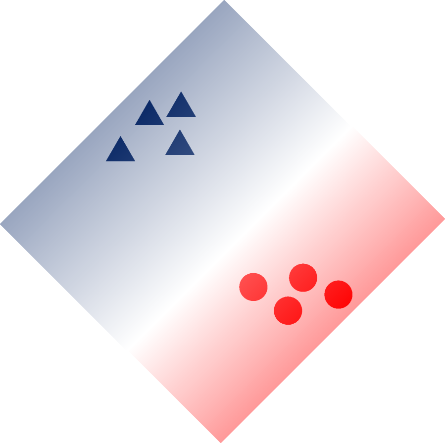
(a) Discriminative

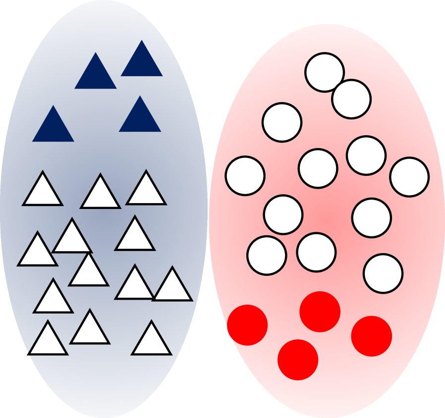
(b) Generative

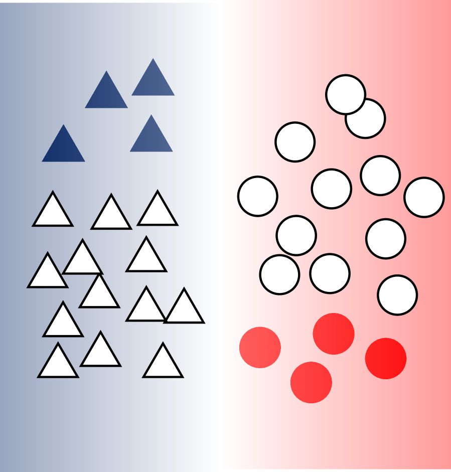
(c) Hybrid

Figure 1: Conceptual diagram of the proposed hybrid model in the application to semi-supervised learning. Blue and red represent classes, and samples filled with each color indicate labeled data, and white samples indicate unlabeled data. The background color represents the posterior probability value or the class conditional distribution obtained by each model. The hybrid model integrates the discriminative power of the discriminative model and the unsupervised data availability of the generative model.

The main contributions of this paper are as follows:

• We realize a hybrid model using a deep discriminative model as the fundamental structure. To achieve this, we propose the Gaussian-coupled softmax layer, which is a softmax layer coupled with Gaussian distributions. By replacing this layer with a softmax layer, a deep discriminative NN can estimate both the class posterior and class-conditional data distributions.

• We expand Minka’s generalization [7] of generative and discriminative models to deep NNs. While retaining the characteristic of their methodology, which is the capability to adjust the strength of the coupling between the generative and discriminative models by the prior distribution of model parameters, we achieved the estimation of a generative model that has the same architecture as the discriminative model utilizing the techniques of the energy-based model (EBM).

• We demonstrate the proposed approach can be applied to tasks associated with classification such as semi-supervised learning and confidence calibration. In particular, we show the effectiveness of the proposed method in medical image recognition, which is a practical task where semi-supervised learning and confidence calibration are effective.

The rest of this paper is organized as follows: Section II describes the background and related studies. The proposed hybrid model and related applications are explained in Section III. The verification of the semi-supervised classification ability using synthetic data and the application to confidence calibration in semi-supervised medical data classification are presented in Section IV. Finally, the conclusion is drawn in Section V.

II Background

II-A Blending Discriminative and Generative Models

The discriminative model is a pattern recognition approach that models the posterior probability $p(\bm{c}\mid\bm{x},\bm{\theta})$, where $\bm{c}$ and $\bm{x}$ represent random variables for the class label and input data, respectively, and $\bm{\theta}$ denotes the model parameter. Given a training dataset comprising $N$ samples $\mathbf{X}=\{\bm{x}_{1},\ldots,\bm{x}_{N}\}$ along with labels $\mathbf{C}=\{\bm{c}_{1},\ldots,\bm{c}_{N}\}$, our objective is to predict the posterior probability $p(\hat{\bm{c}}\mid\hat{\bm{x}},\mathbf{X},\mathbf{C})$ for estimating the class label $\hat{\bm{c}}$ for a newly given sample $\hat{\bm{x}}$. To learn the model parameter $\bm{\theta}$, the following joint distribution is maximized:

$$p(\bm{\theta},\mathbf{C}\mid\mathbf{X})=p(\bm{\theta})\prod^{N}_{n=1}p(\bm{c}_{n}\mid\bm{x}_{n},\bm{\theta}).$$ (1)

The generative model is defined based on the joint distribution of the data $\bm{x}$ and the class label $\bm{c}$, $p(\bm{x},\bm{c}\mid\bm{\theta})$. The parameter $\bm{\theta}$ is learned by maximizing the joint likelihood as

$$p(\mathbf{X},\mathbf{C},\bm{\theta})=p(\bm{\theta})\prod^{N}_{n=1}p(\bm{x}_{n},\bm{c}_{n}\mid\bm{\theta}).$$ (2)

In general, the discriminative model exhibits better classification performance than the generative model. In contrast, the generative model can handle unsupervised data and shows calibrated confidence.

Although each model is generally adopted independently, the two models can be generalized by considering the following model family with an additional set of parameters $\widetilde{\bm{\theta}}$ [7]:

$$q(\bm{x},\bm{c}\mid\bm{\theta},\widetilde{\bm{\theta}})=p(\bm{c}\mid\bm{x},\bm{\theta})p(\bm{x}\mid\widetilde{\bm{\theta}}),$$ (3)

where

$$p(\bm{x}\mid\widetilde{\bm{\theta}})=\sum_{\bm{c^{\prime}}}p(\bm{x},\bm{c^{\prime}}\mid\widetilde{\bm{\theta}}).$$ (4)

Here, $p(\bm{c}\mid\bm{x},\bm{\theta})$ represents the discriminative model and $p(\bm{x}\mid\widetilde{\bm{\theta}})$ is the generative model, but with a different set of parameters $\widetilde{\bm{\theta}}$. The joint likelihood can be expressed by defining a joint prior of the parameters, $p(\bm{\theta},\widetilde{\bm{\theta}})$, as follows:

$$q(\mathbf{X},\mathbf{C},\bm{\theta},\widetilde{\bm{\theta}})=p(\bm{\theta},\widetilde{\bm{\theta}})\prod^{N}_{n=1}p(\bm{c}_{n}\mid\bm{x}_{n},\bm{\theta})p(\bm{x}_{n}\mid\widetilde{\bm{\theta}})$$ (5)

In this modeling, the joint prior $p(\bm{\theta},\widetilde{\bm{\theta}})$ controls the dependence of $\bm{\theta}$ and $\widetilde{\bm{\theta}}$. If the prior factorizes as $p(\bm{\theta},\widetilde{\bm{\theta}})=p(\bm{\theta})p(\widetilde{\bm{\theta}})$, the two models are independent; hence, the resulting value of $\bm{\theta}$ becomes identical to a discriminative model that is trained independently. However, if $p(\bm{\theta},\widetilde{\bm{\theta}})$ has a strong correlation, the values of $\bm{\theta}$ and $\widetilde{\bm{\theta}}$ approximate each other. Namely, the joint prior tunes how the discriminative and generative models are blended.

Why is blending important? A hybrid model that blends the generative and discriminative models has the potential of outperforming its generative and discriminative extremes. Of course, if the generative model could represent the real data generation process perfectly, it should show better performance than its discriminative counterpart. In real-world classification problems, there is a mismatch between the true distribution of the data and the model, and that is why discriminative models that are more flexible generally outperform generative models. Conversely, the advantages of the generative model are that it can use unlabeled data for training in addition to labeled data and that it shows calibrated confidence. The hybrid model inherits the advantages of both models. For example, Lasserre et al. [8] applied a hybrid model to object recognition and showed that the best generalization occurs in the intermediate between the generative and discriminative extremes.

II-B Energy-based Model (EBM)

An EBM is a generative model that specifically models only a negative log-probability called the energy function instead of modeling a normalized probability. The probability density function is formulated by normalizing the energy function as $p_{\bm{\theta}}(\bm{x})=\exp(-E_{\bm{\theta}}(\bm{x}))/Z_{\bm{\theta}}$, where $E_{\bm{\theta}}$ represents the energy function parameterized with $\bm{\theta}$ and $Z_{\bm{\theta}}$ denotes the normalizing term calculated as $Z_{\bm{\theta}}=\int_{\bm{x}}\exp(-E_{\bm{\theta}}(\bm{x}))\mathrm{d}\bm{x}$. In general, the integral in the normalizing term is intractable. Its estimation is one of the difficulties of EBMs and sampling methods such as the Markov chain Monte Carlo method (MCMC) and stochastic gradient Langevin dynamics (SDLG) [11] are often used.

II-C Confidence Calibration

Confidence calibration is the problem of predicting probability estimates that are representative of the true correctness likelihood [12]. A classifier is considered to be calibrated if the posterior probability of the predicted class aligns with its classification rate. For example, when a calibrated classifier predicts a label with a confidence of 0.8, it should have an 80% of chance of being correct. The perfect confidence is defined as follows:

$$p(\hat{Y}=Y\mid\hat{P}=p)=p,\quad\forall p\in[0,1],$$ (6)

where $\hat{Y}$ and $\hat{P}$ represent a class prediction and its associated confidence, respectively.

The common metric for evaluating the calibration algorithm is the expected calibration error (ECE). ECE is defined as $\mathrm{ECE}=\sum^{M}_{m=1}\frac{|B_{m}|}{n}\left|\mathrm{acc}(B_{m})-\mathrm{conf}(B_{m})\right|$, where $n$ represents the number of samples, and $B_{m}$ is the set of indices of the samples whose prediction confidence falls into the interval $I_{m}=(\frac{m-1}{M},\frac{m}{M}]$. Functions $\mathrm{acc}(B_{m})$ and $\mathrm{conf}(B_{m})$ are the accuracy of $B_{m}$ and the average confidence within $B_{m}$, which are respectively defined as $\mathrm{acc}(B_{m})=\frac{1}{|B_{m}|}\sum_{i\in B_{m}}1(\hat{y}_{i}=y_{i})$, where $\hat{y}_{i}$ and $y_{i}$ denote the predicted and true class labels for the $i$-th sample, and $\mathrm{conf}(B_{m})=\frac{1}{|B_{m}|}\sum_{i\in B_{m}}\hat{p}_{i}$, where $\hat{p}_{i}$ represents the predicted confidence for the $i$-th sample.

II-D Related Work

II-D1 Hybrid Models

Various studies on hybrid models have been conducted aiming at complementary use of the characteristics of the discriminative and generative models. Minka [7] generalized the generative and discriminative models and pointed out that the difference of these models is brought from the strength of the constraints on the parameters. Lasserre et al. [8] proposed a semi-supervised learning method based on the findings by Minka. McCallum et al. [13] formulated a hybrid model based on a different approach from [7] and [8]. Druck et al. [14] applied McCallum’s method [13] to semi-supervised learning. Perina et al. [15] proposed a hybrid model based on free-energy terms.

Hybrid models using deep NNs have also been investigated in recent years. Grathwohl et al. [16] considered the final softmax layer of an NN as an energy-based model and proposed a method to learn generative and discriminative models simultaneously, thereby revealing the applicability of the hybrid model to confidence calibration, data generation, and outlier detection. Tu [17] proposed a method for creating a generative model using a discriminative model. Qiao et al. [18] performed semi-supervised learning by collaborative learning of two types of NNs, where the two NNs are trained adversarially. Kuleshov and Ermon [9] proposed a hybrid model using deep NNs and generalized a hybrid model utilizing latent variables, which is equivalent to the mathematical organization of Kingma et al. [19]’s semi-supervised variational auto-encoder. Roth et al. [20] constructed a hybrid model based on a Gaussian mixture model and applied it to semi-supervised learning. Gordon and Hernández-Lobato [10] proposed a hybrid model based on Bayesian deep learning and applied it to semi-supervised learning.

In contrast to these conventional studies, the proposed method can be applied to any NN structure that has a softmax layer at the final layer. Moreover, the proposed method blends the discriminative and generative models and can tune the strength of the characteristics of the two models by the prior distribution of model parameters.

II-D2 Energy-based Models

EBMs involve a wide range of applications such as image generation [21, 22], texture generation [23], text generation [24, 25], compositional generation, memory modeling, protein design and folding, outlier detection, confidence calibration, adversarial robustness, semi-supervised learning [16], reinforcement learning, and continual learning. Du et al. [26] improved the training stability of EBMs by introducing KL divergence between the MCMC kernel and model distribution. They also showed that data augmentation and multi-scale processing can be used to improve robustness and generation quality.

The generative model part of the proposed Gaussian-coupled softmax layer can be regarded as a special case of the EBM when jointly trained with a deep NN. The resulting structure is similar to that of the joint energy-based model (JEM) [16] and details on the differences between them are discussed in the following section.

II-D3 Confidence Calibration

Since calibrated confidence is important in the real-world decision making process, many researchers have investigated confidence calibration. In particular, the confidence calibration for modern deep NNs are explored recently. Guo et al. [12] first explored the confidence calibration for modern deep NNs and found that a simple calibration method using a single parameter called temperature scaling was effective for many datasets. Seo et al. [27] proposed a confidence calibration method for deep NNs based on stochastic inference. Mehrtash et al. [28] proposed a confidence calibration method for medical image segmentation using a deep NN. Wang et al. [29] proposed a confidence calibration method for graph NNs.

Most of the existing methods are called post-hoc calibration, which calibrates the confidence of an already trained model. The proposed method differs from them in that it aims to obtain a calibrated confidence at training time, thereby allowing the use in combination with existing post-hoc calibration methods.

III Hybrid of Discriminative and Generative Models

III-A Gaussian-coupled Softmax Layer

The key idea of the proposed method is a novel layer called a Gaussian-coupled softmax layer, which allows the network to learn generative and discriminative models simultaneously. This layer uses the relationship between the softmax layer and Gaussian distribution, where the parameters of both models can be associated by a simple trick using Bayes’ theorem, and simultaneously learns the generative model paired with the softmax layer. Specifically, the proposed method sets a prior distribution on the parameter space of both models to cooperate with each other.

Regarding the problem of classifying the input vector $\bm{x}\in\mathbb{R}^{D}$ into one of the classes $c\in\{1,\cdots,C\}$, where $C$ denotes the number of classes, the proposed Gaussian-coupled softmax layer consists of a softmax layer that outputs the class posterior probability and Gaussian distributions that calculate the class conditional distribution:

$$p(c\mid\bm{x},\bm{\theta})=\frac{\exp({\bm{w}_{c}}^{\top}\bm{x}+b_{c})}{\sum^{C}_{c^{\prime}=1}\exp({\bm{w}_{c^{\prime}}}^{\top}\bm{x}+b_{c^{\prime}})},$$ (7)

$$p(\bm{x},\!c\!\mid\!\widetilde{\bm{\theta}})\!=\!\frac{\pi_{c}}{(2\pi)^{\frac{D}{2}}{|{\bf\Sigma}|}^{\frac{1}{2}}}\!\exp{\!\left[\!-\frac{1}{2}(\bm{x}\!-\!\bm{\mu}_{c})^{\top}\!{\bf\Sigma}^{-1}\!(\bm{x}\!-\!\bm{\mu}_{c})\!\right]},$$ (8)

where $\bm{\theta}=\{\bm{w}_{c},b_{c}\}_{c=1}^{C}$ is a set of parameters for the discriminative model that consists of a weight $\bm{w}_{c}\in\mathbb{R}^{D}$ and a bias term $b_{c}\in\mathbb{R}$, $\widetilde{\bm{\theta}}=\{\{\pi_{c},\bm{\mu}_{c}\}_{c=1}^{C},{\bf\Sigma}\}$ is the generative model parameter set, $\pi_{c}$ and $\bm{\mu}_{c}\in\mathbb{R}^{D}$ represent the prior and mean vectors for class $c$, respectively, and ${\bf\Sigma}\in\mathbb{R}^{D\times D}$ is the covariance matrix shared among all the classes.

III-B Parameter association

To cooperate two different models in the parameter space, we consider the association of parameters between the discriminative and generative models. We use a simple trick using Bayes’ theorem for this. To align the left-hand side of Eq. (8) with that of Eq. (7), we calculate the class posterior probabilities using Eq. (8) and Bayes’ theorem as follows:

$$p(c\!\mid\!\bm{x},\!\widetilde{\bm{\theta}}) \!=\!\frac{p(\bm{x},c\!\mid\!\widetilde{\bm{\theta}})}{\sum_{c^{\prime}=1}^{C}p(\bm{x},c^{\prime}\!\mid\!\widetilde{\bm{\theta}})}$$

$$\!=\!\frac{\exp{\left[\bm{\mu}_{c}^{\top}{\bf\Sigma}^{-1}\bm{x}\!+\!\ln\pi_{c}-\frac{1}{2}\bm{\mu}_{c}^{\top}{\bf\Sigma}^{-1}\bm{\mu}_{c}\right]}}{\sum_{c^{\prime}=1}^{C}\!\exp{\left[\bm{\mu}_{c^{\prime}}^{\top}{\bf\Sigma}^{-1}\bm{x}\!+\!\ln\pi_{c^{\prime}}\!-\!\frac{1}{2}\bm{\mu}_{c^{\prime}}^{\top}{\bf\Sigma}^{-1}\bm{\mu}_{c^{\prime}}\right]}}.$$ (9)

The second-order terms and some constant terms are canceled out because the covariance matrix ${\bf\Sigma}\in\mathbb{R}^{D\times D}$ is common to all the classes (details are described in Appendix A).

Comparing Eqs. (7) and (III-B) indicates that they have a similar formulation although the parameters are different. Specifically, $\bm{w}_{c}$ and $\bm{{\bf\Sigma}^{-1}\mu}_{c}$, and $b_{c}$ and $\ln\pi_{c}-\frac{1}{2}\bm{\mu}_{c}^{\top}{\bf\Sigma}^{-1}\bm{\mu}_{c}$ are associated with each other. In the model learning, the discriminative and generative models are cooperated by setting a joint prior that correlates the associated parameters.

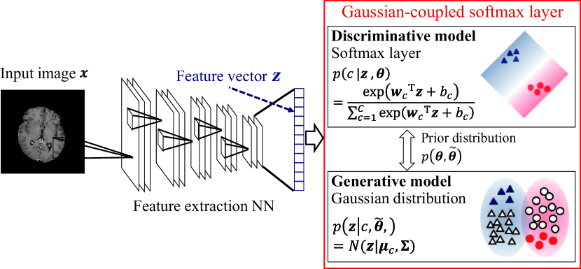
Figure 2: Schematic diagram of joint learning of a deep NN and the Gaussian-coupled softmax layer. Given an input image, a feature vector is extracted by a feature extraction NN. The Gaussian-coupled softmax layer receives the feature vector and outputs the posterior and class-conditional data distributions by discriminative and generative models, respectively. Learning is performed by setting a prior distribution, such that the corresponding parameters between generative and discriminative models have a correlation.

III-C Hybrid Model Learning

In the model learning stage, the discriminative and generative models adopt different evaluation functions; however, they learn so that the associated parameters between both models cooperate with each other. Specifically, the discriminative model learns based on the posterior probability maximization, and the generative model learns based on the joint probability maximization, while setting the joint prior distribution $p(\bm{\theta},\widetilde{\bm{\theta}})$, such that the parameters $\bm{\theta}$ and $\widetilde{\bm{\theta}}$ are mutually correlated. That is, for the given training data set $\{\bm{x}_{n},c_{n}\}_{n=1}^{N}$, the parameters $\bm{\theta}$ and $\widetilde{\bm{\theta}}$ are obtained by maximizing the following likelihood function.

$$p(\bm{\theta},\widetilde{\bm{\theta}})\prod_{n=1}^{N}p(\bm{c}_{n}|\bm{x}_{n},\bm{\theta})p(\bm{x}_{n}|\widetilde{\bm{\theta}})$$ (10)

The joint prior distribution $p(\bm{\theta},\widetilde{\bm{\theta}})$ is set so that $\bm{\theta}$ and $\widetilde{\bm{\theta}}$ have a correlation. In this paper, we propose the use of the following joint prior:

$$p(\bm{\theta},\widetilde{\bm{\theta}}) =\prod_{c=1}^{C}\mathcal{N}(\bm{w}_{c}\mid\bm{{\bf\Sigma}^{-1}\mu}_{c},\lambda^{-1}{\bf I})$$

$$\quad\cdot\mathcal{N}(b_{c}\mid\ln\pi_{c}-\frac{1}{2}\bm{\mu}_{c}^{\top}{\bf\Sigma}^{-1}\bm{\mu}_{c},\lambda^{-1})p(\widetilde{\bm{\theta}})$$ (11)

where $\mathcal{N}(\cdot)$ is a Gaussian distribution, ${\bf I}\in\mathbb{R}^{D\times D}$ is an identity matrix, the precision $\lambda$ is a hyperparameter that adjusts the variance of the prior distribution, and $p(\widetilde{\bm{\theta}})$ is a non-informative prior distribution. Using this prior, $\log p(\bm{\theta},\widetilde{\bm{\theta}})$ can be attributed to the norm of associated parameters:

$$\log p(\bm{\theta},\widetilde{\bm{\theta}})$$

$$\!=\!-\frac{\lambda}{2}\sum_{c=1}^{C}\left\{\left\|\bm{w}_{c}\!-\!\bm{{\bf\Sigma}^{-1}\mu}_{c}\right\|^{2}\!+\!\left\|b_{c}\!+\!\frac{1}{2}\bm{\mu}_{c}^{\top}{\bf\Sigma}^{-1}\bm{\mu}_{c}\right\|^{2}\!\right\}.$$ (12)

Here, constant terms are ignored. The hybrid model learning is accomplished by adding Eq. (III-C) to the loss in addition to the respective training of discriminative/generative models.

III-D Joint Learning with a Deep Neural Network

Fig. 2 shows a schematic diagram of joint learning with a deep NN. The proposed Gaussian-coupled softmax layer can be trained with a deep NN in an end-to-end manner. Let $\bm{z}_{n}=f_{\bm{\phi}}(\bm{x}_{n})$ be the feature vector extracted from a deep NN $f$ parameterized with $\bm{\phi}$ given an input $\bm{x}_{n}$, and the Gaussian-coupled softmax layer receives $\bm{z}_{n}$ as an input. We here redefine $\bm{\theta}$ and $\widetilde{\bm{\theta}}$ so that they include the NN parameter $\bm{\phi}$ in addition to the original parameters.

The log-likelihood function for a sample $\bm{x}_{n}$ can be formulated as follows:

$$\log p(\bm{\theta},\widetilde{\bm{\theta}})+\log p(\bm{c}_{n}|\bm{x}_{n},\bm{\theta})+\log p(\bm{x}_{n}|\widetilde{\bm{\theta}}).$$ (13)

The first term consists of only parameters and can be attributed to the norm of parameters as described in Eq. (III-C). The second term is a negative cross-entropy that is generally used for discriminative model training. The third term cannot be computed in a straightforward manner because of the use of feature extraction net $f_{\bm{\phi}}(\bm{x}_{n})$; hence, we use the following formulation using an intractable normalizing term:

$$p(\bm{x}_{n}|\widetilde{\bm{\theta}})=\sum_{c}\exp{\left(-E_{\widetilde{\bm{\theta}}}(\bm{x}_{n};c)\right)}/Z_{\widetilde{\bm{\theta}}},$$ (14)

where $E_{\widetilde{\bm{\theta}}}(\bm{x}_{n};c)=\frac{1}{2}(\bm{z}_{n}-\bm{\mu}_{c})^{\top}{\bf\Sigma}^{-1}(\bm{z}_{n}-\bm{\mu}_{c})$. The normalizing term $Z_{\widetilde{\bm{\theta}}}=\int\exp{\left(-E_{\widetilde{\bm{\theta}}}^{\mathrm{total}}(\bm{x}_{n})\right)}\mathrm{d}x$, where $E_{\widetilde{\bm{\theta}}}^{\mathrm{total}}(\bm{x}_{n})=-\log\sum_{c}\exp(-E_{\widetilde{\bm{\theta}}}(\bm{x}_{n};c))$. The gradient of $\log p(\bm{x}_{n}|\widetilde{\bm{\theta}})$ with respect to $\widetilde{\bm{\theta}}$ can be calculated as follows:

$$\frac{\partial\log p(\bm{x}_{n}|\widetilde{\bm{\theta}})}{\partial\widetilde{\bm{\theta}}}\!=\!\mathbb{E}_{p_{\widetilde{\bm{\theta}}}(\bm{x^{\prime}})}\left[\frac{\partial E_{\widetilde{\bm{\theta}}}^{\mathrm{total}}(\bm{x^{\prime}})}{\partial\widetilde{\bm{\theta}}}\right]\!-\!\frac{\partial E_{\widetilde{\bm{\theta}}}^{\mathrm{total}}(\bm{x}_{n})}{\partial\widetilde{\bm{\theta}}},$$ (15)

where the expectation is calculated via sampling from the estimated distribution using SGLD [11].

$$\bm{x}_{0} \sim p_{0}(\bm{x}),$$

$$\bm{x}_{i+1} =\bm{x}_{i}+\frac{\alpha}{2}\frac{\partial E_{\widetilde{\bm{\theta}}}^{\mathrm{total}}(\bm{x}_{i})}{\partial\bm{x}_{i}}+\epsilon,\quad\epsilon\sim\mathcal{N}(0,\alpha),$$ (16)

where $p_{0}$ is the initial distribution that is typically a uniform distribution and $\alpha$ is the step size.

Discussion. The joint learning of the proposed Gaussian softmax layer with a Deep NN and JEM [16] have similar structures. The critical difference is that JEM uses exactly the same parameters for the discriminative and generative models; therefore it cannot blend and balance the two models. Conversely, the proposed method has different parameters for both models and can adjust the correlation between two models with a joint prior distribution. This allows us to tune the strength of the characteristics of the discriminative and generative models depending on the task.

III-E Applications

Semi-supervised learning. The proposed hybrid model can learn unlabeled data as well as labeled data, while the conventional NN-based discriminative model can only handle labeled data. Given sets of indices for labeled and unlabeled data, $D_{\mathrm{L}}$ and $D_{\mathrm{U}}$, respectively, semi-supervised learning using the proposed method is attributed to a maximization problem of the following likelihood function.

$$p(\bm{\theta},\widetilde{\bm{\theta}})\prod_{n=1}^{N}p(\bm{c}_{n}|\bm{x}_{n},\bm{\theta})p(\bm{x}_{n}|\widetilde{\bm{\theta}})$$

$$\!=\!p(\bm{\theta},\widetilde{\bm{\theta}})\!\!\left[\prod_{n\in D_{\text{L}}}\!\!p\left(\bm{c}_{n}|\bm{x}_{n},\bm{\theta}\right)p(\bm{x}_{n}|\bm{c}_{n},\bm{\widetilde{\theta}})\!\right]\!\!\!\left[\prod_{m\in D_{\text{U}}}\!\!\!p(\bm{x}_{m}|\widetilde{\bm{\theta}})\!\right]$$ (17)

Confidence calibration. The NN trained with the proposed method is expected to exhibit calibrated confidence. The confidence, which is the maximum value of the posterior probability that a classifier outputs, is important in applications of machine learning such as medical diagnosis, where the confidence is used to evaluate the uncertainty of a decision. In the general training using the cross-entropy loss, the confidence often becomes inaccurate. This is because the cross-entropy loss can be further minimized by increasing the confidence even after the model is able to correctly classify almost all training samples, resulting in an overconfident model [12]. In particular, semi-supervised learning tends to produce inaccurate confidence, which adversely affects the final decision-making in actual diagnostic applications. To obtain accurate confidence, it is necessary to accurately estimate the data distribution $p(x)$, in addition to the discrimination boundary.

Data generation. The proposed method can be applied to synthetic data generation because it involves the estimation of the generative model, despite the classifier architecture. This characteristic allows the user to confirm whether the model correctly estimated the input data distribution from the generated data. Synthetic data are generated via sampling based on the SGLD algorithm. Specifically, the data are generated by exploring the input space while sampling the data so that the generative model part, $p(\bm{x})$, outputs a higher value. The quality of the generated data itself is not as high as that of models specialized in data generation such as GANs and VAEs. This is because the proposed method is basically a classifier and not structured to output synthetic data given noise input. Examples of generated images are shown in Appendix C.

IV Experiments

IV-A Verification Using Synthetic Data

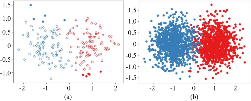
Figure 3: Synthetic data for verification. Blue and red indicate Classes 1 and 2, respectively. (a) Training data. The white circles are unlabeled samples whose contour colors correspond to the true labels, and the circles filled in blue or red are labeled samples. (b) Test data.

To verify the validity of the proposed method, we performed an experiment on semi-supervised classification of synthetic data. Fig. 3 shows the synthetic data for this experiment. The data comprises two classes and are generated from Gaussian distributions with different means for each class. The averages for Classes 1 and 2 were $[0,-0.5]^{\top}$ and $[0,0.5]^{\top}$, respectively, and the covariance matrix was $\bigl{[}\begin{smallmatrix}0.5&0\\ 0&0.5\end{smallmatrix}\bigr{]}$, which was shared by both classes. In the training data, labels were assigned only to the five points with the highest $y$-coordinate values for Class 1 and five points with the lowest $y$-coordinate values for Class 2. This was intended to set up a problem in which a decision boundary that is significantly different from the correct one is obtained if only the labeled data were employed. The numbers of training and test data were 100 and 1,000 samples, respectively. We repeated the experiments ten times while regenerating the training and test data and calculated an average accuracy.

We used the proposed Gaussian-coupled softmax layer stand-alone, i.e., we directly input the data into the proposed layer without using any other NN for feature extraction. The prior distribution $P(\bm{\theta},\widetilde{\bm{\theta}})$ shown in equation (III-C) with a precision parameter $\lambda=10$ was used. Stochastic gradient descent with a learning rate of $0.001$ was used for optimization. For comparison, we used a softmax layer as a simple discriminative model and trained the model with only the labeled data and with all the training data labeled (i.e., a fully supervised situation).

Fig. 4 shows examples of the discrimination results for the test data. As confirmed in Fig. 4(a), when learning was performed only with the discriminative model, the decision boundary was significantly different from the ideal boundary, and the accuracy was greatly reduced. In Fig. 4(b), the proposed method showed a decision boundary close to the ideal boundary, and the accuracy was almost the same as that of fully supervised learning shown in Fig. 4(c). The average accuracies of ten trials for the discriminative model only, hybrid model, and fully supervised learning were $89.72~{}(3.842)$%, $97.54~{}(0.3507)$%, $97.32~{}(0.4723)$%, respectively, where the values in parentheses indicate standard deviations.

These results indicate that the proposed method properly used the distribution information of unlabeled samples, suggesting the applicability of the proposed method to semi-supervised learning. This experiment was performed under ideal conditions where the feature values of each class follow a normal distribution. The same condition can be realized if a feature extractor can acquire the features that follow the Gaussian distribution according to the generative model.

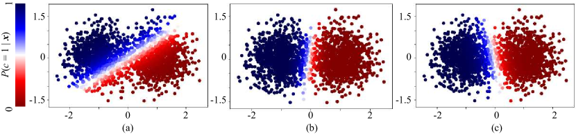
Figure 4: Discrimination results for the synthetic data. (a) Discriminative model only (accuracy: 82.6 %), (b) Hybrid model (ours) (accuracy: 97.4 %), (c) Fully supervised learning (accuracy: 97.4 %). The colors in the figure indicate the class 1 posterior probabilities for each sample.

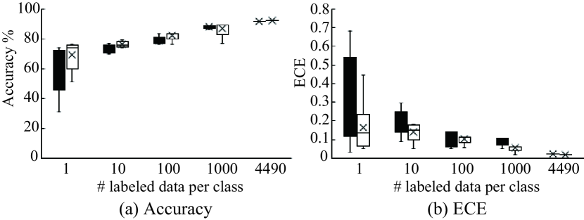
Figure 5: Results of medical data classification. (a) Accuracy. (b) Expected calibration error (ECE). In each panel, black and white bars represent the baseline and proposed method, respectively.

TABLE I: Results for the MedMNIST dataset. Values in parentheses indicate standard deviations.

			# labeled data per class = 1				# labeled data per class = 10
Dataset	Criterion		Baseline	JEM	Ours		Baseline	JEM	Ours
Blood	ACC (%)$\uparrow$		46.72 (4.978)	48.19 (9.631)	52.31 (3.336)		74.21 (1.710)	65.93 (20.70)	77.71 (2.920)
	ECE (%)$\downarrow$		39.08 (8.444)	24.55 (15.98)	19.68 (5.109)		22.18 (2.715)	19.25 (26.64)	2.626 (0.652)
Derma	ACC (%)$\uparrow$		28.24 (11.78)	36.12 (10.43)	40.89 (16.12)		49.99 (2.220)	58.99 (3.215)	61.04 (4.791)
	ECE (%)$\downarrow$		56.26 (18.95)	23.38 (8.818)	18.11 (5.270)		40.88 (5.674)	24.58 (9.340)	18.41 (3.575)
OrganA	ACC (%)$\uparrow$		34.24 (3.894)	40.37 (5.193)	40.04 (5.064)		66.56 (2.428)	71.87 (1.879)	74.89 (1.646)
	ECE (%)$\downarrow$		53.70 (2.437)	18.27 (4.990)	27.91 (12.51)		27.82 (1.101)	5.684 (1.074)	2.582 (1.406)
OrganC	ACC (%)$\uparrow$		28.16 (3.466)	33.47 (7.056)	34.15 (6.103)		62.12 (1.282)	68.02 (3.161)	73.07 (2.744)
	ECE (%)$\downarrow$		60.06 (5.543)	18.65 (8.823)	13.78 (4.765)		31.68 (0.786)	9.796 (1.974)	6.275 (4.451)
OrganS	ACC (%)$\uparrow$		25.30 (1.296)	28.50 (4.522)	22.43 (1.831)		48.078 (2.786)	54.52 (2.459)	53.45 (7.873)
	ECE (%)$\downarrow$		61.60 (4.047)	23.47 (12.11)	13.81 (10.64)		43.70 (2.316)	15.81 (4.209)	10.36 (2.916)
Pneumonia	ACC (%)$\uparrow$		54.04 (9.849)	62.53 (0.064)	64.74 (6.750)		80.90 (3.790)	81.70 (4.477)	81.28 (2.990)
	ECE (%)$\downarrow$		25.67 (18.84)	23.36 (12.01)	20.90 (13.25)		11.87 (5.181)	11.84 (5.247)	11.33 (3.722)

IV-B Confidence Calibration in Semi-supervised Medical Data Classification

As an application of the proposed hybrid model, we conducted medical data classification experiments to evaluate the effectiveness for confidence calibration in semi-supervised learning. Semi-supervised learning is useful for medical data classification. In the process of applying machine learning-based pattern recognition to medical diagnosis, we first annotate the collected medical data and train a classifier. The trained classifier outputs the class posterior probability for newly obtained data. The output posterior probabilities are then used to assist doctors in diagnosis. However, annotation of medical data requires specialized knowledge and is expensive. Therefore, semi-supervised learning is often utilized where only a part of the data is annotated and the majority of the data is unsupervised. In addition, the confidence should be calibrated because the doctor refers to the confidence of the classifier outputs. Furthermore, it can be applied to confidence-based active learning if the confidence is appropriately calibrated.

We first analyzed the behavior of the proposed method using small-scale data. In this analysis, the behavior of the proposed method with respect to the changes in the number of labeled data and the precision parameter $\lambda$ was confirmed. After that, we conducted a comparative experiment using publicly available medical datasets.

IV-B1 Behavior Analysis Using Small-scale Data

We prepared an MR image classification dataset from the multimodal brain tumor image segmentation benchmark (BraTS) [30]. Details for this dataset are described in Appendix B.

To evaluate the effectiveness for semi-supervised learning, we randomly reduced the number of labeled samples for each class to 1,000, 100, 10, and 1. We used the wide residual network (wide-ResNet) [31] for the feature extraction network of the proposed hybrid model; the Gaussian-coupled softmax layer was connected to the wide-ResNet as the last layer removing the softmax layer from the original architecture. We used the wide-ResNet with the softmax layer as the baseline method. We calculated expected calibration error (ECE) [12] as well as classification accuracy. For the proposed method and the baseline, we used the ADAM optimizer with a learning rate of 0.0001 and set the number of epochs to 150. For the proposed method, we set the number of steps to 100, $\alpha=2.0$, and $\epsilon=0.01$ for the SGLD.

The accuracy and ECE in the MRI classification for each number of labeled samples are shown in Fig. 5. This figure is a box plot of ten-time repetitions by changing labeled data. Both methods exhibited improvement in both accuracy and ECE as the number of labeled data increased. The proposed method tends to be better than the baseline for all sample sizes, and the difference is noticeable when the number of labeled data is small. This suggests that the proposed method is more effective when the number of labeled data is small.

Fig. 6 presents the accuracy and ECE when the precision parameter $\lambda$ was varied. In this figure, we used 100 samples of labeled data. Fig. 6(a) shows that the accuracy is not so sensitive to the change of $\lambda$, but it decreases when $\lambda$ is set extremely large or small. ECE, however, decreases as $\lambda$ is increased. This is because the hybrid model becomes closer to the generative model when $\lambda$ is increased.

Figure 6: Accuracy and ECE for each value of precision parameter $\lambda$.

IV-B2 Comparison Using Benchmark Datasets

We also conducted a comparison using MedMNIST [32]. MedMNIST is a large-scale collection of medical image datasets that contains 18 datasets for various tasks. We picked up six datasets (BloodMNIST, DermaMNIST, OrganAMNIST, OrganCMNIST, OrganSMNIST, and PneumoniaMNIST) that are suitable for semi-supervised classification. We performed the experiments for the cases where the number of labeled data was one and ten. We used the same evaluation metrics, feature extraction network, baseline, and parameters as the previous section except for $\lambda$, which is set based on the validation set. We compared the results with those of the baseline and JEM.

The results are shown in Table I. The proposed method outperformed the baseline and JEM in terms of accuracy on average. Furthermore, the proposed method remarkably improved the ECE.

To analyze the remarkable improvement in the ECE, we visualized the confidence histogram and reliability diagram in Fig. 7. This figure is from the results for BloodMNIST with ten samples of labeled data per class. In Fig. 7(a), the baseline outputs a confidence close to 1 for most of the samples. This is a typical overconfidence problem that general discriminative models fall into. In contrast, the proposed method in Fig. 7(b) showed a less biased confidence histogram and well-calibrated reliability diagram.

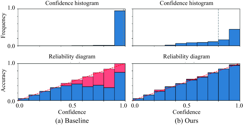
Figure 7: Confidence histogram and reliability diagrams for BloodMNIST classification. In the confidence histogram, the black dashed line represents the average confidence. In the reliability diagram, blue and red rectangles show the actual average accuracy in each bin and the gap to the ideal, respectively.

V Conclusion

In this paper, we proposed a method to train a hybrid of generative and discriminative models in a single neural network (NN). The key idea is the Gaussian-coupled softmax layer, which is a softmax layer coupled with Gaussian distributions. By replacing this layer with a softmax layer, a deep discriminative NN can estimate both the class posterior distribution and the class-conditional data distribution. In the experiments, we demonstrated the effectiveness of the proposed method for semi-supervised classification and confidence calibration.

Limitation. Although the proposed hybrid model can be combined with any differentiable NN in principle, the difficulty of learning (ease of divergence) depends on the network structure. Based on our experience, the wide ResNet (and similar networks such as the ResNet) is easy to control, and a deep LSTM for time-series data is also applicable. However, networks that have complex architectures such as an attention module are difficult to control.

In future work, we will explore further applications. The potential applications include outlier detection, missing value imputation, and time-series forecasting.

Appendix A Derivation of Eq. (III-B)

The details of deriving Eq. (III-B) expression in section III-A are as follows.

$$P(c\mid\bm{x})$$

$$=\frac{P(c)P(\bm{x}\mid c)}{\sum_{c^{\prime}=1}^{C}P(c^{\prime})P(\bm{x}\mid c^{\prime})}$$

$$=\frac{\pi_{c}(2\pi)^{-\frac{D}{2}}{|{\bf\Sigma}|}^{-\frac{1}{2}}\exp{\left[-\frac{1}{2}(\bm{x}-\bm{\mu}_{c})^{\rm T}{\bf\Sigma}^{-1}(\bm{x}-\bm{\mu}_{c})\right]}}{\sum_{c^{\prime}=1}^{C}\pi_{c^{\prime}}(2\pi)^{-\frac{D}{2}}{|{\bf\Sigma}|}^{-\frac{1}{2}}\exp{\left[-\frac{1}{2}(\bm{x}-\bm{\mu}_{c^{\prime}})^{\rm T}{\bf\Sigma}^{-1}(\bm{x}-\bm{\mu}_{c^{\prime}})\right]}}$$

$$=\frac{\exp{\left[\ln\pi_{c}-\frac{1}{2}\bm{x}^{\mathrm{T}}{\bf\Sigma}^{-1}\bm{x}+\bm{\mu}_{c}^{\mathrm{T}}{\bf\Sigma}^{-1}\bm{x}-\frac{1}{2}\bm{\mu}_{c}^{\mathrm{T}}{\bf\Sigma}^{-1}\bm{\mu}_{c}\right]}}{\sum_{c^{\prime}=1}^{C}\exp{\left[\ln\pi_{c^{\prime}}-\frac{1}{2}\bm{x}^{\mathrm{T}}{\bf\Sigma}^{-1}\bm{x}+\bm{\mu}_{c^{\prime}}^{\mathrm{T}}{\bf\Sigma}^{-1}\bm{x}-\frac{1}{2}\bm{\mu}_{c^{\prime}}^{\mathrm{T}}{\bf\Sigma}^{-1}\bm{\mu}_{c^{\prime}}\right]}}$$

$$=\frac{\exp{\left[\bm{\mu}_{c}^{\mathrm{T}}{\bf\Sigma}^{-1}\bm{x}+\ln\pi_{c}-\frac{1}{2}\bm{\mu}_{c}^{\mathrm{T}}{\bf\Sigma}^{-1}\bm{\mu}_{c}\right]}}{\sum_{c^{\prime}=1}^{C}\exp{\left[\bm{\mu}_{c^{\prime}}^{\mathrm{T}}{\bf\Sigma}^{-1}\bm{x}+\ln\pi_{c^{\prime}}-\frac{1}{2}\bm{\mu}_{c^{\prime}}^{\mathrm{T}}{\bf\Sigma}^{-1}\bm{\mu}_{c^{\prime}}\right]}}$$ (18)

Appendix B Details for MRI Dataset

We prepared an MR image dataset from the multimodal brain tumor image segmentation benchmark (BraTS) [30]. This dataset consisted of three-dimensional brain MR images with tumor annotation and was originally provided for tumor segmentation. We created an image classification dataset by horizontally slicing 3D volume data into axial 2D images. We then separated the images into tumor and non-tumor classes based on the existence of the tumor annotation. The dataset contained 220 subjects, and we randomly divided these into 154, 22, and 44 for training, validation, and testing, respectively. Consequently, we obtained 8,980, 1,448, and 2,458 images for training, validation, and testing, respectively because approximately 60 images were extracted from each subject. We resized the images from $240\times 240$ pixels to $32\times 32$ due to computational limitations.

Appendix C Data Generation

As described in Section III-E, the proposed method can generate synthetic data, and this characteristic can be used to confirm whether the model correctly estimated the input data distribution. We show some examples of generated images for the MedMNIST dataset in Figs. 8–13. In each figure, ten generated images are randomly selected for each class and aligned in a row.

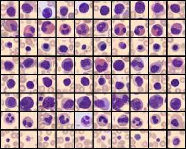
Figure 8: Generated images for BloodMNIST.

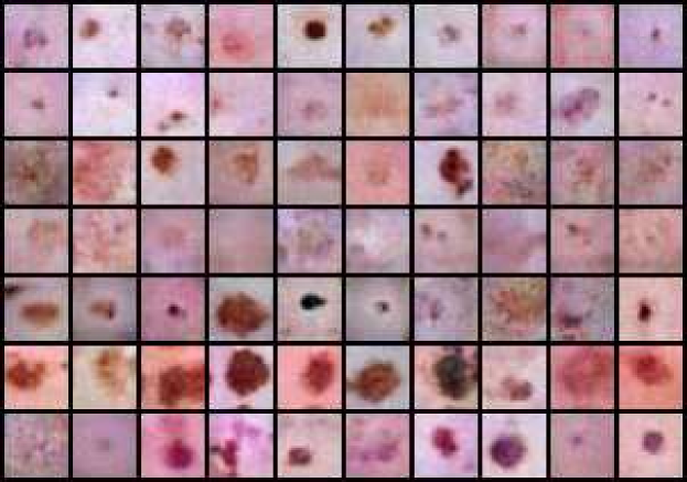
Figure 9: Generated images for DermaMNIST.

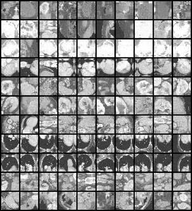
Figure 10: Generated images for OrganAMNIST.

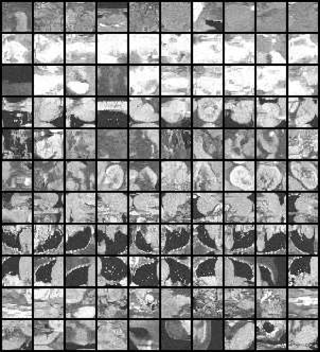
Figure 11: Generated images for organCMNIST.

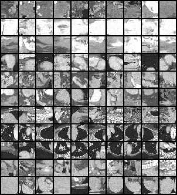
Figure 12: Generated images for OrganSMNIST.

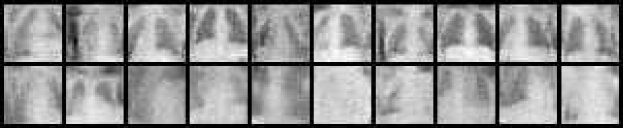
Figure 13: Generated images for PneumoniaMNIST.

References

- [1] M. Ehsan Abbasnejad, A. Dick, and A. van den Hengel, “Infinite variational autoencoder for semi-supervised learning,” in Proc. Conf. Comput. Vis. Pattern Recog. (CVPR), 2017, pp. 5888–5897.
- [2] S. Akcay, A. Atapour-Abarghouei, and T. P. Breckon, “Ganomaly: Semi-supervised anomaly detection via adversarial training,” in Proc. Asian Conf. Comput. Vis. (ACCV), 2018, pp. 622–637.
- [3] K. Lee, H. Lee, K. Lee, and J. Shin, “Training confidence-calibrated classifiers for detecting out-of-distribution samples,” in Proc. Int. Conf. Learn. Represent. (ICLR), 2018.
- [4] I. Goodfellow, J. Pouget-Abadie, M. Mirza, B. Xu, D. Warde-Farley, S. Ozair, A. Courville, and Y. Bengio, “Generative adversarial nets,” in Proc. Adv. Neural Inform. Process. Syst. (NIPS), vol. 27, 2014.
- [5] D. P. Kingma and M. Welling, “Auto-encoding variational Bayes,” in Proc. Int. Conf. Learn. Represent. (ICLR), 2014.
- [6] D. Rezende and S. Mohamed, “Variational inference with normalizing flows,” in Proc. Int. Conf. Mach. Learn. (ICML), 2015, pp. 1530–1538.
- [7] T. Minka, “Discriminative models, not discriminative training,” MSR-TR-2005-144, Microsoft Research, Tech. Rep., 2005.
- [8] J. A. Lasserre, C. M. Bishop, and T. P. Minka, “Principled hybrids of generative and discriminative models,” in Proc. Conf. Comput. Vis. Pattern Recog. (CVPR), 2006, pp. 87–94.
- [9] V. Kuleshov and S. Ermon, “Deep hybrid models: Bridging discriminative and generative approaches,” in Proc. Conf. Uncertainty Artif. Intell. (UAI), 2017.
- [10] J. Gordon and J. M. Hernández-Lobato, “Combining deep generative and discriminative models for bayesian semi-supervised learning,” Pattern Recognition, vol. 100, p. 107156, 2020.
- [11] M. Welling and Y. W. Teh, “Bayesian learning via stochastic gradient Langevin dynamics,” in Proc. Int. Conf. Mach. Learn. (ICML), 2011, pp. 681–688.
- [12] C. Guo, G. Pleiss, Y. Sun, and K. Q. Weinberger, “On calibration of modern neural networks,” in Proc. Int. Conf. Mach. Learn. (ICML), 2017, pp. 1321–1330.
- [13] A. McCallum, C. Pal, G. Druck, and X. Wang, “Multi-conditional learning: Generative/discriminative training for clustering and classification,” in Proc. AAAI Conf. Artif. Intell. (AAAI), 2006, pp. 433–439.
- [14] G. Druck, C. Pal, A. McCallum, and X. Zhu, “Semi-supervised classification with hybrid generative/discriminative methods,” in Proc. Int. Conf. Knowledge Discovery and Data Mining (KDD), 2007, pp. 280–289.
- [15] A. Perina, M. Cristani, U. Castellani, V. Murino, and N. Jojic, “A hybrid generative/discriminative classification framework based on free-energy terms,” in Proc. Int. Conf. Comput. Vis. (ICCV), 2009, pp. 2058–2065.
- [16] W. Grathwohl, K.-C. Wang, J.-H. Jacobsen, D. Duvenaud, M. Norouzi, and K. Swersky, “Your classifier is secretly an energy based model and you should treat it like one,” in Proc. Int. Conf. Learn. Represent. (ICLR), 2020.
- [17] Z. Tu, “Learning generative models via discriminative approaches,” in Proc. Conf. Comput. Vis. Pattern Recog. (CVPR), 2007.
- [18] S. Qiao, W. Shen, Z. Zhang, B. Wang, and A. Yuille, “Deep co-training for semi-supervised image recognition,” in Proc. Europ. Conf. Comput. Vis. (ECCV), 2018, pp. 135–152.
- [19] D. P. Kingma, S. Mohamed, D. Jimenez Rezende, and M. Welling, “Semi-supervised learning with deep generative models,” in Proc. Adv. Neural Inform. Process. Syst. (NIPS), vol. 27, 2014.
- [20] W. Roth, R. Peharz, S. Tschiatschek, and F. Pernkopf, “Hybrid generative-discriminative training of Gaussian mixture models,” Pattern Recognition Letters, vol. 112, pp. 131–137, 2018.
- [21] T. Han, E. Nijkamp, X. Fang, M. Hill, S.-C. Zhu, and Y. N. Wu, “Divergence triangle for joint training of generator model, energy-based model, and inferential model,” in Proc. Conf. Comput. Vis. Pattern Recog. (CVPR), 2019, pp. 8670–8679.
- [22] Y. Du and I. Mordatch, “Implicit generation and modeling with energy based models,” in Proc. Adv. Neural Inform. Process. Syst. (NeurIPS), vol. 32, 2019.
- [23] J. Xie, Y. Lu, R. Gao, and Y. N. Wu, “Cooperative learning of energy-based model and latent variable model via MCMC teaching,” in Proc. AAAI Conf. Artif. Intell. (AAAI), vol. 32, no. 1, 2018.
- [24] Y. Deng, A. Bakhtin, M. Ott, A. Szlam, and M. Ranzato, “Residual energy-based models for text generation,” in Proc. Int. Conf. Learn. Represent. (ICLR), 2020.
- [25] A. Bakhtin, Y. Deng, S. Gross, M. Ott, M. Ranzato, and A. Szlam, “Residual energy-based models for text,” Journal of Mach. Learn. Research, vol. 22, no. 40, pp. 1–41, 2021.
- [26] Y. Du, S. Li, B. J. Tenenbaum, and I. Mordatch, “Improved contrastive divergence training of energy based models,” in Proc. Int. Conf. Mach. Learn. (ICML), 2021.
- [27] S. Seo, P. H. Seo, and B. Han, “Learning for single-shot confidence calibration in deep neural networks through stochastic inferences,” in Proc. Conf. Comput. Vis. and Pattern Recog. (CVPR), 2019, pp. 9030–9038.
- [28] A. Mehrtash, W. M. Wells, C. M. Tempany, P. Abolmaesumi, and T. Kapur, “Confidence calibration and predictive uncertainty estimation for deep medical image segmentation,” IEEE Trans. Med. Imag., vol. 39, no. 12, pp. 3868–3878, 2020.
- [29] X. Wang, H. Liu, C. Shi, and C. Yang, “Be confident! towards trustworthy graph neural networks via confidence calibration,” Proc. Adv. Neural Inform. Process. Syst. (NeurIPS), vol. 34, 2021.
- [30] B. H. Menze, A. Jakab, S. Bauer, J. Kalpathy-Cramer, K. Farahani, J. Kirby, Y. Burren, N. Porz, J. Slotboom, R. Wiest et al., “The multimodal brain tumor image segmentation benchmark (BRATS),” IEEE Trans. Med. Imag., vol. 34, no. 10, pp. 1993–2024, 2014.
- [31] S. Zagoruyko and N. Komodakis, “Wide residual networks,” arXiv preprint arXiv:1605.07146, 2016.
- [32] J. Yang, R. Shi, D. Wei, Z. Liu, L. Zhao, B. Ke, H. Pfister, and B. Ni, “MedMNIST v2: A large-scale lightweight benchmark for 2D and 3D biomedical image classification,” arXiv preprint arXiv:2110.14795, 2021.