Revisit the entanglement entropy with gravitational anomaly

Abstract

In this paper we study the entanglement entropy in the CFT₂, whose gravity dual is AdS₃ spacetime with a Chern-Simons term. Using the generalized Rindler method, we obtain the Rindler transformation in the two-dimensional planar CFT and compute the entanglement entropy of the CFT with gravitational anomalies. The conditions under which the entanglement entropy may have anomalous contributions is also discussed. In addition, we present a relatively general form of the Rindler AdS metric and compute its thermal entropy, which agrees with the entanglement entropy in the field theory. Moreover, we utilize the conformal transformation, which maps a cylinder to a plane, to compute the entanglement entropy of the CFT residing on a cylinder, as well as the entanglement entropy of the CFT at finite temperature on a plane. The corresponding contribution of the Chern-Simons term in gravity to the black hole thermal entropy is also obtained from this approach. These results are important for further understandings of the two-dimensional CFT with gravitational anomalies.

1 Introduction

Quantum entanglement is a quantum phenomenon that has no classical counterpart RevModPhys.81.865 . Entanglement entropy is a measure of quantum entanglement that reflects how entanglement is stored in quantum states. For instance, the Hilbert space of a biparticle system can be written as the product of two factors

$$\mathcal{H}=\mathcal{H}_{A}\otimes\mathcal{H}_{\bar{A}},$$ (1)

where $\mathcal{H}_{A}$ and $\mathcal{H}_{\bar{A}}$ are the Hilbert space of the two subsystems $A$ and $\bar{A}$, respectively. The von Neumann entropy $S_{A}$ of the subsystem $A$ is defined as

$$S_{A}=-\mathrm{Tr}\rho_{A}\log\rho_{A},\qquad\rho_{A}=\mathrm{Tr}_{\bar{A}}\rho$$ (2)

where $\rho$ is the density matrix of the total system. $S_{A}$ is also called the entanglement entropy hartman2015lectures . In a continuous QFT, if the space is divided into two parts $A$ and $B$, with the boundary $\partial A$, the computation of the entanglement entropy is not easy since the result is divergent Calabrese:2004eu ; Calabrese:2009qy . A UV cutoff must be introduced to obtain a finite result. Entanglement entropy in the two-dimensional conformal field theory (CFT) is an active area of research, in which the entanglement entropy can be systematically calculated in many cases Calabrese:2004eu , such as:

• A CFT sits on an infinite plane, and consider an interval $A$ of length $\ell$ on this plane. Its entanglement entropy is

  $$S_{A}\sim(c/3)\log(\ell/a),$$ (3)

  Where $c$ is the central charge of the CFT and $a$ is the UV cutoff.

• For the case when $A$ is a single interval of length $\ell$, and periodic boundary conditions are imposed on the whole system, that is to say, CFT lives on a cylinder. One can find

  $$S_{A}\sim(c/3)\log((L/\pi a)\sin(\pi\ell/L)),$$ (4)

  where $L$ is the circumference of the circle at the base of the cylinder.

• Consider a spatial interval $A$ with length $\ell$ on a plane at a finite temperature $\beta^{-1}.$ The CFT now resides on a cylinder with a compact thermal cycle, i.e., the topology is $M=S^{1}\times\mathbb{R}.$ The entanglement entropy of $A$ is

  $$S_{A}\sim(c/3)\log((\beta/\pi a)\sinh(\pi\ell/\beta)).$$ (5)

For higher-dimensional CFT, the calculation of entanglement entropy becomes more complex and challenging. Fortunately, Ryu and Takayanagi Ryu:2006bv ; Ryu:2006ef ; Hubeny:2007xt proposed that the calculation of entanglement entropy can be transformed into the calculation of the area of a minimal surface in gravity through the AdS/CFT correspondence Maldacena:1997re ; Witten:1998qj . Specifically, entanglement entropy $S_{A}$ in CFT_d+1 can be computed from the following area law relation

$$S_{A}=\frac{\operatorname{Area}\left(\gamma_{A}\right)}{4G_{N}^{(d+2)}},$$ (6)

where $\gamma_{A}$ is the minimal surface in $AdS_{d+2}$ with boundary $\partial A$. The area of $\gamma_{A}$ is denoted as Area$(\gamma_{A})$, and $G_{N}^{(d+2)}$ is the Newton constant in $d+2$-dimensional gravity. When this method is applied to AdS₃, Ryu and Takayanagi perfectly reproduced the entanglement entropy in two-dimensional CFT Ryu:2006bv .

However, proving the Ryu-Takayanagi formula (6) or holographic entanglement entropy formula is not an easy task. Fursaev was the first to make some attempts Fursaev:2006ih , but unfortunately there are some problems in his calculations. Subsequently, the authors of Casini:2011kv found that considering the spherical entanglement surface in CFT can map this spherical region to a hyperbolic geometry through conformal transformation. The vacuum state is mapped to the thermal state in the hyperbolic geometry. Then, according to the AdS/CFT correspondence, the entanglement entropy of the original CFT can be calculated by calculating the thermal entropy in gravity. With this idea, the holographic entanglement entropy formula for the special case of a spherical entanglement surface was proven. A more general proof was provided by Lewkowycz and Maldacena Lewkowycz:2013nqa , who employed the Euclidean gravitational path integral method. This approach has become a powerful tool for understanding holographic entanglement entropy and was later extended to demonstrate covariant holographic entanglement entropy Dong:2016hjy . For further information, please see references Nishioka:2018khk ; Rangamani:2016dms .

It should be noted that Lewkowycz and Maldacena’s method appears to rely heavily on the AdS/CFT correspondence and may not be easily extended to other holographic theories. On the other hand, the conformal transformation method in reference Casini:2011kv is more readily applicable to other holographic theories and has been used for entanglement entropy in Warped Conformal Field Theory Castro:2015csg . However, finding the transformation from the vacuum state to the thermal state can be challenging. The problem of finding the transformation from the vacuum state to the thermal state has been solved in the cases where the boundary is a two-dimensional field theory Song:2016gtd ; Jiang:2017ecm . The authors of references Song:2016gtd ; Jiang:2017ecm named their method of finding this transformation as the generalized Rindler method. This is also the method that will be used in this paper, and we will review it in Section 3.1.

For the usual AdS₃/CFT₂, the operation of calculating (or deriving) holographic entanglement entropy using the generalized Rindler method is shown in Fig. 1.

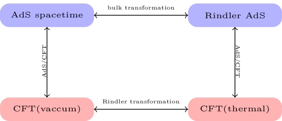
Figure 1: A schematic diagram illustrating the relationship between gravity, field theory, and their connections in the study of holographic entanglement entropy using the generalized Rindler method

The process of the operation is as follows:

• Calculate the Killing vector field of AdS₃. On the asymptotic boundary, the global conformal transformation generators in the boundary CFT can be obtained from the Killing vector fields.

• Once the global conformal transformation generators are obtained, the Rindler transformation in the field theory can be calculated using the generalized Rindler method (see Section 3.1). This transformation maps the entanglement entropy in the CFT to the thermal entropy in another CFT. By directly calculating the thermal entropy, the entanglement entropy can be obtained. This is also a method for calculating entanglement entropy directly in field theory without relying on holography.

• The bulk transformation can be obtained from the Rindler transformation in field theory according to the generalized Rindler method. The bulk transformation transforms AdS₃ into Rindler AdS₃. By calculating the black hole entropy of Rindler AdS₃ (equivalent to calculating the black hole area), the thermal entropy of the thermal CFT can be obtained. The black hole area is directly related to the area of the minimal surface through the bulk transformation.

In this paper, we aim to calculate the entanglement entropy in a CFT where the left-moving central charge is not equal to the right-moving central charge ($c_{L}\neq c_{R}$) using the generalized Rindler method. Specifically, we consider a bulk action containing a Chern-Simons term, i.e., topologically massive gravity (TMG), with a CFT on the boundary where $c_{L}\neq c_{R}$. The holographic entanglement entropy in this case has been discussed in Jiang:2019qvd ; Castro:2014tta ; Sun:2008uf , and the Rindler method has also been discussed by the author in Jiang:2019qvd . Here, we will give a more detailed discussion. Kraus:2005zm shows that even when a Chern-Simons term is added to the bulk action, global AdS₃ remains a solution to the bulk. Therefore, all our derivations will start from global AdS₃. An important feature of the entanglement entropy in a CFT with gravitational anomaly is the presence of a Lorentzian anomaly. In Section 3.3, we will show how to derive the anomalous term in the entanglement entropy from the calculation of the thermal entropy in the field theory. For more information on holographic gravitational anomaly and entanglement entropy in a CFT with gravitational anomaly, please refer to Castro:2014tta ; Kraus:2005zm .

The organization of this paper is as follows: In Sec. 2, we will briefly review the AdS₃ spacetime and find out its Killing vector fields, which correspond to the generators of the conformal group of the two-dimensional CFT on the boundary. In Sec. 3, we will introduce how to use the Rindler method to calculate the entanglement entropy of a two-dimensional CFT with gravitational anomaly in field theory. In particular, we will carefully deal with the UV cutoffs in order to analyze the anomalous contribution of the entanglement entropy in detail. In Sec. 4, we will derive the Rindler transformation in the bulk and calculate the thermal entropy of Rindler AdS. In Sec. 5, we will derive the entanglement entropy of a zero-temperature CFT on a cylinder and a finite-temperature CFT on a plane. We will give a summary of this paper in Sec. 6.

2 AdS₃ and Killing vector fields

A fundamental property of AdS spacetime is that the isometry group of a $(d+1)$-dimensional AdS spacetime is identical to the conformal group of a $d$-dimensional Minkowski spacetime. This is a significant finding in the study of AdS/CFT correspondence, which suggests that Killing vector fields in the bulk are related to the generators of global conformal symmetry on the boundary. We start with the flat four-dimensional space $\mathbb{R}^{2,2}$, whose metric is

$$ds^{2}=-dy_{0}^{2}-dy_{1}^{2}+dy_{2}^{2}+dy_{3}^{2},\qquad G_{ab}=\text{diag}(-1,-1,1,1).$$ (7)

One can immediately obtain the Killing vector fields of this metric, which correspond to two types of transformations, namely, rotations and boosts. Their explicit forms are given as follows PhysRevD.59.104001 ; Natsuume:2014sfa ; hartman2015lectures

$$\text{Rotation:}\qquad L_{ab} = y_{a}\partial_{b}-y_{b}\partial_{a},\qquad ab=01,23$$ (8)

$$\text{Boost:}\qquad J_{ab} = y_{a}\partial_{b}+y_{b}\partial_{a},\qquad ab=02,03,12,13$$ (9)

and these generators form the group $SO(2,2)$. The AdS₃ can be embedded into this flat spacetime via

$$-L^{2}=-y^{2}_{0}-y^{2}_{1}+y^{2}_{2}+y^{2}_{3},$$ (10)

where $L$ is the AdS radius, and we will set it to $L=1$ in the remainder of this paper. As AdS₃ possesses $SO(2,2)$ symmetry, we can obtain its Killing vector fields by “restricting” the previously obtained Killing vector fields to AdS₃. The procedure is as follows: Assume that the manifolds $M=(\text{AdS}_{3},g_{ab})$ and $N=(\mathbb{R}^{2,2},G_{ab})$, and suppose there exists a smooth mapping $\phi:M\rightarrow N$ such that for all $p\in M$, we have $\phi(p)\in N$. If there exists a coordinate system $\{x^{\alpha}\}\equiv\{x^{0},x^{1},x^{2}\}$ in a neighborhood of point $p$ in $M$, and a coordinate system $\{y^{\mu}\}\equiv\{y^{0},y^{1},y^{2},y^{3}\}$ in a neighborhood of point $\phi(p)$ in $N$, then the Killing vector fields in $M$ and $N$ are related as follows

$$\tilde{K}^{a}=\tilde{K}^{\alpha}\left(\frac{\partial}{\partial x^{\alpha}}\right)^{a}=g^{\alpha\beta}\left(\phi^{\ast}K\right)_{\beta}\left(\frac{\partial}{\partial x^{\alpha}}\right)^{a}=g^{\alpha\beta}\frac{\partial y^{\mu}}{\partial x^{\beta}}G_{\mu\nu}K^{\nu}\left(\frac{\partial}{\partial x^{\alpha}}\right)^{a}.$$ (11)

Here, $\tilde{K}^{a}$ is a Killing vector field “restricted” in AdS₃ and $K^{a}$ is a Killing vector field in $\mathbb{R}^{2,2}$. The expression $(\phi^{\ast}K)_{a}$ represents the pullback of the dual vector $K_{a}$ under the map $\phi$. We define

$$L_{1}=\left(-L_{01}+L_{23}\right)/2,\quad L_{2}=\left(J_{12}-J_{03}\right)/2,\qquad L_{3}=\left(J_{02}+J_{13}\right)/2,$$ (12)

$$\bar{L}_{1}=\left(-L_{01}-L_{23}\right)/2,\quad\bar{L}_{2}=\left(J_{12}+J_{03}\right)/2,\qquad\bar{L}_{3}=\left(J_{02}-J_{13}\right)/2.$$ (13)

One can easily check that:

$$\left[L_{1},L_{2}\right]=-L_{3};\quad\left[L_{1},L_{3}\right]=L_{2};\quad\left[L_{2},L_{3}\right]=L_{1},$$ (14)

$$\left[\bar{L}_{1},\bar{L}_{2}\right]=-\bar{L}_{3};\quad\left[\bar{L}_{1},\bar{L}_{3}\right]=\bar{L}_{2};\quad\left[\bar{L}_{2},\bar{L}_{3}\right]=\bar{L}_{1}.$$ (15)

Then, we redefine

$$L_{0}=L_{2},\qquad L_{-}=L_{1}+L_{3},\qquad L_{+}=L_{1}-L_{3},$$ (16)

$$\bar{L}_{0}=\bar{L}_{2},\qquad\bar{L}_{-}=\bar{L}_{1}+\bar{L}_{3},\qquad\bar{L}_{+}=\bar{L}_{1}-\bar{L}_{3}.$$ (17)

One can readily verify that the new Killing vector fields satisfy the Lie algebra of $SL(2,L)$ and $SL(2,R)$, respectively,

$$SL(2,L): \qquad\left[L_{0},L_{\pm}\right]=\mp L_{\pm},\qquad\left[L_{+},L_{-}\right]=2L_{0},$$ (18)

$$SL(2,R): \qquad\left[\bar{L}_{0},\bar{L}_{\pm}\right]=\mp\bar{L}_{\pm},\qquad\left[\bar{L}_{+},\bar{L}_{-}\right]=2\bar{L}_{0}.$$ (19)

By making the following coordinate transformation, we can relate the hypersurface defined by (10) to the Poincaré coordinates in the AdS₃ spacetime Casini:2011kv :

$$y_{0}+y_{3}=\frac{L^{2}}{z},\qquad y_{1}=\frac{L}{z}t,\qquad y_{2}=\frac{L}{z}x.$$ (20)

Together with the defining equation of the hypersurface (10), we totally have four equations, from which we can solve for $y^{\mu}\equiv y_{\mu}$ in terms of $y_{\mu}(x^{\alpha})$. To facilitate later calculations, we perform another coordinate transformation in this paper:

$$u=x+t,\qquad v=x-t.$$ (21)

The induced metric on the hypersurface is:

$$ds^{2}=\frac{1}{z^{2}}\left(dz^{2}+dudv\right).$$ (22)

Taking the asymptotic limit as $z\rightarrow 0$ and removing the $1/z^{2}$ factor, we obtain the metric for the dual CFT living on the boundary. Using equation (11), we can obtain the Killing vector fields in AdS₃ that corresponds to the Killing vector fields given in equations (16) and (17), namely:

$$\tilde{L}_{0} = u\partial_{u}+\frac{z}{2}\partial_{z},\qquad\tilde{L}_{+}=-\partial_{u},\qquad\tilde{L}_{-}=-u^{2}\partial_{u}+z^{2}\partial_{v}-uz\partial_{z},$$ (23)

$$\tilde{\bar{L}}_{0} = -v\partial_{v}-\frac{z}{2}\partial_{z},\qquad\tilde{\bar{L}}_{+}=-z^{2}\partial_{u}+v^{2}\partial_{v}+vz\partial_{z},\qquad\tilde{\bar{L}}_{-}=\partial_{v}.$$ (24)

On the asymptotic boundary, the global generators of the conformal transformation are

$$l_{0}=u\partial_{u},\qquad l_{+}=-\partial_{u},\qquad l_{-}=-u^{2}\partial_{u},$$ (25)

$$\bar{l}_{0}=-v\partial_{v},\qquad\bar{l}_{+}=v^{2}\partial_{v},\qquad\bar{l}_{-}=\partial_{v}.$$ (26)

With these ingredients, we can use the generalized Rindler method Casini:2011kv to solve the holographic entanglement entropy in AdS₃/CFT₂.

3 Entanglement entropy from field theory

In this section, we will investigate the entanglement entropy of a two-dimensional CFT with gravitational anomalies using the generalized Rindler method. To this end, we will first provide a brief overview of the Rindler method. For detailed information, please refer to references Casini:2011kv ; Castro:2015csg ; Song:2016gtd ; Jiang:2017ecm .

3.1 (Generalized) Rindler method

The main idea of the Rindler method is to use a symmetry transformation to transform the calculation of entanglement entropy in field theory to the calculation of thermal entropy. In the context of holography, the thermal entropy of the boundary field theory is related to the black hole entropy in the bulk. Therefore, the entanglement entropy in field theory can be calculated by computing the black hole entropy in gravity from the Rindler method. The key to the Rindler method is to find the appropriate Rindler transformation. The main approach to find the Rindler transformation has been summarized in reference Jiang:2017ecm , and we will provide a brief introduction here.

Assuming that the quantum field theory on the manifold $B$ is invariant under the group $G$, and the generators of the global symmetries in the group $G$ are denoted by $h_{i}$. If we want to calculate the entanglement entropy of a subregion $A$, then the Rindler transformation $R$ is a symmetry transformation that maps the causal domain of $A$, which is denoted as $\mathcal{D}$, to a non-compact manifold $\tilde{B}$. The Rindler transformation $R$ here should satisfy:

1. Rindler transformation

   $$\left.\begin{array}[]{c}R:\mathcal{D}\rightarrow\tilde{B}\\ \quad~{}x\mapsto\tilde{x}\\ \end{array}\right.$$ (27)

   is a symmetry transformation. Here $x=\left(x^{0},x^{1}\right)\in\mathcal{D}$, $\tilde{x}=\left(\tilde{x}^{0},\tilde{x}^{1}\right)\in\tilde{B}$.

2. The new coordinates should satisfy $\tilde{x}^{i}\sim\tilde{x}^{i}+i\tilde{\beta}^{i}$ in order to obtain a thermal state.

3. The vectors $\partial_{\tilde{x}^{i}}$ annihilate vacuum, that is

   $$\partial_{\tilde{x}^{i}}=\sum_{j}b_{ij}h_{j},$$ (28)

   where $b_{ij}$ are arbitrary constants.

4. Let $k_{t}=\tilde{\beta}^{i}\partial_{\tilde{x}^{i}}$ be the generator of the modular flow, such that the causal domain remains invariant under this flow for the selected region.

Under these conditions, the Rindler transformation can be derived. In the next subsection, we will apply the Rindler method to provide a detailed calculation of the entanglement entropy in field theory. The holographic dictionary tells us that the global generators of the asymptotic symmetry group correspond to the isometry generators of the bulk metric. By substituting the generators of the bulk isometries for the $h_{i}$ generators, and requiring the Rindler bulk space to satisfy the same boundary conditions, we can obtain the Rindler transformations in the bulk spacetime.

3.2 Rindler transformation in CFT₂

In this section, we will demonstrate how to use the Rindler method to calculate the entanglement entropy of a subsystem in a CFT. This calculation can also be found in referencesSong:2016gtd ; Jiang:2017ecm ; Wen:2018whg , but our presentation will be more detailed than previous works.

Consider a region $\mathcal{I}$ in a zero-temperature CFT on a plane, which can be described by the following equation:

$$\mathcal{I}\equiv\left\{\left(u,v\right)\bigg{|}u=l_{u}\left(s-\frac{1}{2}\right),v=l_{v}\left(s-\frac{1}{2}\right),s\in\left[0,1\right]\right\},$$ (29)

where $l_{u}$ and $l_{v}$ are some positive constants which restrict the domain of dependence (DOD) of $\mathcal{I}$ to

$$\mathcal{D}=\left\{\left(u,v\right)\bigg{|}-\frac{l_{u}}{2}<u<\frac{l_{u}}{2},-\frac{l_{v}}{2}<v<\frac{l_{v}}{2}\right\}.$$ (30)

According to the Rindler method, we can map this region to a thermal state via a conformal transformation. Assuming that this conformal transformation is

$$u^{\prime}=f(u),\qquad v^{\prime}=g(v).$$ (31)

In the field theory, the Rindler transformation is

$$u^{\prime}=\frac{\beta_{u^{\prime}}}{\pi}\arctan\!\text{h}\frac{2u}{l_{u}},$$ (32)

$$v^{\prime}=-\frac{\beta_{v^{\prime}}}{\pi}\arctan\!\text{h}\frac{2v}{l_{v}}.$$ (33)

The specific derivation process is given in Appendix A. If we take $\beta_{u^{\prime}}=-\beta_{v^{\prime}}=\pi$, then our Rindler transformation is consistent with the results of reference Wen:2018whg . On the other hand, if we set $l_{u}=l_{v}=2R$, then we have

$$u=R\tanh u^{\prime}=R\frac{1-e^{-2u^{\prime}}}{1+e^{-2u^{\prime}}},$$ (34)

$$v=R\tanh v^{\prime}=R\frac{1-e^{-2v^{\prime}}}{1+e^{-2v^{\prime}}}.$$ (35)

This is formally the same as the equation $(2.31)$ in reference Casini:2011kv , which represents the coordinate transformation that maps the vacuum state to the thermal state. The reason for the lack of exact equivalence is because we have taken $\beta_{u^{\prime}}=-\beta_{v^{\prime}}=\pi$ instead of $\beta_{u^{\prime}}=-\beta_{v^{\prime}}=2\pi$ in the reference Casini:2011kv .

The computation of entanglement entropy in CFT yields a divergent result, and we need to introduce an appropriate cutoff, i.e., a regularization scheme, to compute the entanglement entropy of the region under consideration. Assume the region obtained by truncating $\mathcal{I}$ as

$$\mathcal{I}_{\mathrm{reg}}\equiv\left\{\left.\left(u,v\right)\right.\bigg{|}u=l_{u}\left(s-\frac{1}{2}\right),v=l_{v}\left(s-\frac{1}{2}\right),s\in\left[\varepsilon_{1},1-\varepsilon_{2}\right]\right\}.$$ (36)

After the Rindler transformation similar to the above procedures, $\mathcal{I}_{\mathrm{reg}}$ becomes $\mathcal{I}^{\prime}_{\text{reg}}$:

$$\mathcal{I}_{\mathrm{reg}}^{\prime}=\left\{\left.\left(u^{\prime},v^{\prime}\right)\right.\bigg{|}u^{\prime}=\frac{\beta_{u^{\prime}}}{\pi}\arctan\!\text{h}\left[2\left(s-\frac{1}{2}\right)\right],v^{\prime}=-\frac{\beta_{v^{\prime}}}{\pi}\arctan\!\text{h}\left[2\left(s-\frac{1}{2}\right)\right],s\in\left[\varepsilon_{1},1-\varepsilon_{2}\right]\right\},$$ (37)

where $\varepsilon_{1},\varepsilon_{2}\ll 1$ are the cutoffs. For the convenience, we set

$$\varepsilon_{u1}=l_{u}\varepsilon_{1},\qquad\varepsilon_{u2}=l_{u}\varepsilon_{2},$$ (38)

$$\varepsilon_{v1}=l_{v}\varepsilon_{1},\qquad\varepsilon_{v2}=l_{v}\varepsilon_{2}.$$ (39)

Then we have

$$\frac{\varepsilon_{u1}}{\varepsilon_{v1}}=\frac{\varepsilon_{u2}}{\varepsilon_{v2}}=\frac{l_{u}}{l_{v}}.$$ (40)

This equation reflects the degree to which the interval we consider deviates from the equal time surface (when the interval is on the equal time surface, $l_{u}/l_{v}=1$). Perhaps a more accurate phrasing would be that $l_{u}/l_{v}$ measures the boost of the DOD. We can convert it to the form of boost angle. To this end, we consider a boost that induces a Lorentz transformation (refer to Fig. 2),

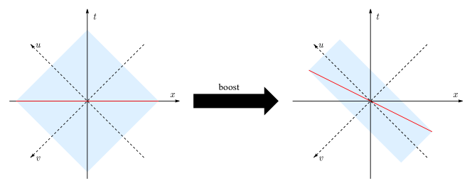
Figure 2: A schematic diagram of an interval (in red) undergoing a boost.

$$t^{\prime} =\gamma\left(t-\nu x\right)=\frac{1}{\sqrt{1-\nu^{2}}}\left(t-\nu x\right),$$ (41)

$$x^{\prime} =\gamma\left(x-\nu t\right)=\frac{1}{\sqrt{1-\nu^{2}}}\left(x-\nu t\right).$$

where $\nu$ is the velocity of the boosted interval relative to the selected inertial frame. Under such a configuration, it can be calculated that

$$\frac{l_{u}}{l_{v}}=e^{-2\kappa}$$ (42)

for the boosted interval, where $\kappa=\arctan\!\text{h}\nu$ is the boost angle.

Here is something that needs to be stressed. The Rindler transformations (32) and (33) are derived for a specific interval $\mathcal{I}$, but they are also applicable to any spacelike curves that have the same DOD. For such a general curve, equations (38) and (39) are not satisfied.

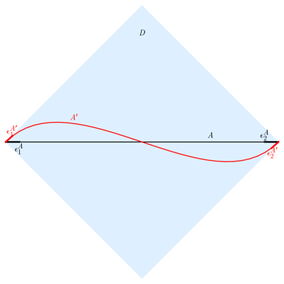
Figure 3: A schematic diagram of different spacelike curves $A$ and $A^{\prime}$ having the same DOD. The $\epsilon^{A,A^{\prime}}_{\#}$’s represent the small truncations at the endpoints of $A$ and $A^{\prime}$ respectively.

As shown in the Fig. 3, there are two spacelike curves, $A$ and $A^{\prime}$, having a common DOD $D$. The $\epsilon^{A,A^{\prime}}_{\#}$’s in the figure are the truncations at the endpoints of $A$ and $A^{\prime}$. For convenience, let’s assume that $\epsilon^{A}_{1}$ and $\epsilon^{A}_{2}$ are boosted to coincide with $\epsilon^{A^{\prime}}_{1}$ and $\epsilon^{A^{\prime}}_{2}$ respectively. We can decompose the truncations of $A^{\prime}$ into truncations in the $u$ and $v$ directions and denoted them as $\epsilon^{A^{\prime}}_{u1},\epsilon^{A^{\prime}}_{v1},\epsilon^{A^{\prime}}_{u2},\epsilon^{A^{\prime}}_{v2}$. They satisfy the following relationship:

$$\frac{\epsilon_{u1}^{A^{\prime}}}{\epsilon_{v1}^{A^{\prime}}} =e^{-2\kappa_{1}},\qquad\frac{\epsilon_{u2}^{A^{\prime}}}{\epsilon_{v2}^{A^{\prime}}}=e^{-2\kappa_{2}},$$ (43)

$$\epsilon_{u1}^{A^{\prime}}\epsilon_{v1}^{A^{\prime}} =\left(\epsilon_{1}^{A}\right)^{2},\qquad\epsilon_{u2}^{A^{\prime}}\epsilon_{v2}^{A^{\prime}}=\left(\epsilon_{2}^{A}\right)^{2},$$

where $\kappa_{1}$ and $\kappa_{2}$ are boost angles of $\epsilon^{A^{\prime}}_{1}$ and $\epsilon_{2}^{A^{\prime}}$, respectively.

3.3 Entanglement entropy of zero temperature CFT on the plane

Consider a CFT living on an arbitrary torus with the following identification

$$\left(\tilde{u},\tilde{v}\right)\sim\left(\tilde{u}+i\bar{a},\tilde{v}-ia\right)\sim\left(\tilde{u}+2\pi\bar{b},\tilde{v}-2\pi b\right),$$ (44)

where $\bar{a},a,\bar{b},b$ are some real constants. Without loss of generality, we assume $\bar{a},\bar{b}>0$. The partition function of the CFT on this torus can be written as $Z_{\bar{b}|b}\left(\bar{a}|a\right)$. It is worth noting that we can always use a Lorentz transformation to turn such an identification into a more “standard” identification. The reason can be briefly summarized as follows: an arbitrary causal region, as shown in the left panel of Fig. 4, can always be transformed into a diamond-shaped region on an equal-time surface through a boost. We may take this equal-time surface to be the $t=0$ surface.

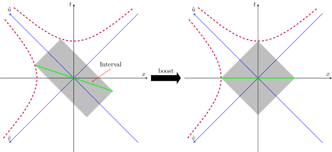
Figure 4: A diagram illustrating the boost transformation of an interval’s DOD into a DOD on an equal-time surface at $t=0$.

Assuming that the coordinates of the leftmost point of the causal region in the left panel of Fig.4 are $(\pi\bar{b},\pi|b|)$, then under the boost this point should move along the curve

$$\tilde{u}=\frac{\pi^{2}|b|\bar{b}}{\tilde{v}}.$$ (45)

The coordinates of the left endpoint in the right panel of Fig.4 should be $(\pi\sqrt{|b|\bar{b}},\pi\sqrt{|b|\bar{b}})$. Setting

$$\tilde{u}^{\prime}=\sqrt{\frac{|b|}{\bar{b}}}\tilde{u},\qquad\tilde{v}^{\prime}=\sqrt{\frac{\bar{b}}{|b|}}\tilde{v}$$ (46)

is equivalent to performing a boost that transforms a boosted DOD into an unboosted DOD. Thus, we can consider the CFT on the following torus

$$\left(\tilde{u}^{\prime},\tilde{v}^{\prime}\right)\sim\left(\tilde{u}^{\prime}+i\sqrt{\frac{\left|b\right|}{\bar{b}}}\bar{a},\tilde{v}^{\prime}-i\sqrt{\frac{\bar{b}}{\left|b\right|}}a\right)\sim\left(\tilde{u}^{\prime}+2\pi\sqrt{\left|b\right|\bar{b}},\tilde{v}^{\prime}-2\pi\operatorname{sgn}\left(b\right)\sqrt{\left|b\right|\bar{b}}\right),$$ (47)

where “$\operatorname{sgn}$” is the sign function. Then we have

$$Z_{\bar{b}|b}\left(\bar{a}|a\right)=Z_{\sqrt{\left|b\right|\bar{b}}|\operatorname{sgn}(b)\sqrt{\left|b\right|\bar{b}}}\left(\sqrt{\frac{\left|b\right|}{\bar{b}}}\bar{a}|\sqrt{\frac{\bar{b}}{\left|b\right|}}a\right).$$ (48)

If we make a scaling transformation

$$\hat{u}=\frac{\tilde{u}^{\prime}}{\sqrt{\left|b\right|\bar{b}}},\qquad\hat{v}=\frac{\tilde{v}^{\prime}}{\sqrt{\left|b\right|\bar{b}}},$$ (49)

we can obtain the usual canonical circle

$$\left(\hat{u},\hat{v}\right)\sim\left(\hat{u}+i\frac{\bar{a}}{\bar{b}},\hat{v}-i\frac{a}{\left|b\right|}\right)\sim\left(\hat{u}+2\pi,\hat{v}-2\pi\text{sgn}\left(b\right)\right),$$ (50)

where the spatial period is $2\pi$. This is still a conformal transformation and the partition function will not change. On the equal-time surface at $t=0$, we can calculate the partition function as in the usual CFT by considering $\hat{u}=\bar{z},\hat{v}=z$, so

$$Z_{\bar{b}|b}\left(\bar{a}|a\right) =Z_{1|\text{sgn}\left(b\right)}\left(\frac{\bar{a}}{\bar{b}}|\frac{a}{\left|b\right|}\right)$$ (51)

$$=\mathrm{Tr}_{1|\text{sgn}\left(b\right)}\left(e^{-\frac{\bar{a}}{\bar{b}}\bar{\mathcal{L}}_{0}^{\mathrm{Cyl}}}e^{\frac{a}{\left|b\right|}\mathcal{L}_{0}^{\mathrm{Cyl}}}\right)=\mathrm{Tr}_{1|\text{sgn}\left(b\right)}\left(e^{-\frac{\bar{a}}{\bar{b}}\left(\bar{\mathcal{L}}_{0}-\frac{c_{L}}{24}\right)}e^{\frac{a}{\left|b\right|}\left(\mathcal{L}_{0}-\frac{c_{R}}{24}\right)}\right),$$

where $\bar{\mathcal{L}}^{\text{Cyl}}_{0},\mathcal{L}_{0}^{\text{Cyl}}$ are the charge of $\partial_{\hat{u}}$ and $\partial_{\hat{v}}$ on the cylinder with the canonical spatial cycle while $\bar{\mathcal{L}}_{0},\mathcal{L}_{0}$ are the charge on a plane. The left-moving central charge $c_{L}$ and right-moving central charge $c_{R}$ of a CFT are generally not equal. The relationship between the second and third equal signs can be found in Blumenhagen:2009zz . Next, we make a conformal transformation to exchange the spatial circle and thermal circle, which is called the S-transformation hartman2015lectures ; DiFrancesco:1997nk ; Blumenhagen:2009zz

$$\hat{u}^{\prime}=2\pi i\frac{\hat{u}}{\beta_{\hat{u}}},\qquad\hat{v}^{\prime}=2\pi i\text{sgn}\left(b\right)\frac{\hat{v}}{\beta_{\hat{v}}},$$ (52)

where we have let $\beta_{\hat{u}}=\frac{\bar{a}}{\bar{b}},\beta_{\hat{v}}=\frac{a}{|b|}$. From this we obtain

$$\left(\hat{u},\hat{v}\right)\sim\left(\hat{u}-2\pi,\hat{v}+2\pi\text{sgn}\left(b\right)\right)\sim\left(\hat{u}+i\frac{4\pi^{2}}{\beta_{\hat{u}}},\hat{v}-i\frac{4\pi^{2}}{\beta_{\hat{v}}}\right).$$ (53)

This is equivalent to replacing $\beta_{\hat{u}}$ with $4\pi^{2}/\beta_{\hat{u}}$ and $\beta_{\hat{v}}$ with $4\pi^{2}/\beta_{\hat{v}}$ in (50). Then we have

$$Z_{1|\text{sgn}\left(b\right)}\left(\frac{\bar{a}}{\bar{b}}|\frac{a}{\left|b\right|}\right)=Z_{1|\text{sgn}\left(b\right)}\left(\beta_{\hat{u}}|\beta_{\hat{v}}\right)=Z_{-1|-\text{sgn}(b)}\left(\frac{4\pi^{2}}{\beta_{\hat{u}}}|\frac{4\pi^{2}}{\beta_{\hat{v}}}\right).$$ (54)

Assume that the contribution of the vacuum to the partition function is dominant, then we arrive

$$Z_{1|\text{sgn}(b)}\left(\beta_{\hat{u}}|\beta_{\hat{v}}\right) =Z_{-1|-\text{sgn}(b)}\left(\frac{4\pi^{2}}{\beta_{\hat{u}}}|\frac{4\pi^{2}}{\beta_{\hat{v}}}\right)$$ (55)

$$=\mathrm{Tr}_{-1|-\text{sgn}(b)}\left(e^{-\frac{4\pi^{2}}{\beta_{\hat{u}}}\left(\bar{\mathcal{L}}_{0}-\frac{c_{L}}{24}\right)}e^{\frac{4\pi^{2}}{\beta_{\hat{v}}}\left(\mathcal{L}_{0}-\frac{c_{R}}{24}\right)}\right)\approx e^{\frac{\pi^{2}c_{L}}{6\beta_{\hat{u}}}}e^{-\frac{\pi^{2}c_{R}}{6\beta_{\hat{v}}}}.$$

Here we have assumed that the vacuum charge on the plane vanishes. Therefore, we can obtain the thermal entropy

$$S_{\bar{b}|b}\left(\bar{a}|a\right) =S_{1|\text{sgn}(b)}\left(\beta_{\hat{u}}|\beta_{\hat{v}}\right)=\left(1-\beta_{\hat{u}}\partial_{\beta_{\hat{u}}}-\beta_{\hat{v}}\partial_{\beta_{\hat{v}}}\right)\log Z_{1|\text{sgn}(b)}\left(\beta_{\hat{u}}|\beta_{\hat{v}}\right)$$ (56)

$$=\left(1-\beta_{\hat{u}}\partial_{\beta_{\hat{u}}}-\beta_{\hat{v}}\partial_{\beta_{\hat{v}}}\right)\left(\frac{\pi^{2}c_{L}}{6\beta_{\hat{u}}}-\frac{\pi^{2}c_{R}}{6\beta_{\hat{v}}}\right)$$

$$=\frac{\pi^{2}}{3}\frac{c_{L}}{\beta_{\hat{u}}}-\frac{\pi^{2}}{3}\frac{c_{R}}{\beta_{\hat{v}}}.$$

It should be noted that our formula is only valid when

$$\beta_{\hat{u}}\rightarrow 0^{+},\qquad\beta_{\hat{v}}\rightarrow 0^{-}.$$ (57)

The most general formula for the thermal entropy of CFT on an arbitrary torus can be obtained through the same operation,

$$S_{\bar{b}|b}\left(\bar{a}|a\right)=\frac{\pi^{2}}{3}\frac{c_{L}}{\beta_{\hat{u}}}+\frac{\pi^{2}}{3}\frac{c_{R}}{\beta_{\hat{v}}},$$ (58)

where $\beta_{\hat{u}}=\left|\bar{a}/\bar{b}\right|$, $\beta_{\hat{v}}=\left|a/b\right|$. The equation (58), known as the Cardy formula Cardy:1986ie ; Hartman:2014oaa , applies to the case when $\beta_{\hat{u}}\rightarrow 0$ and $\beta_{\hat{v}}\rightarrow 0$.

From (37), we obtain

$$\left|\bar{a}\right| = \left|\beta_{u^{\prime}}\right|,\qquad\qquad\qquad\qquad\left|a\right|=\left|\beta_{v^{\prime}}\right|,$$ (59)

$$2\pi\left|\bar{b}\right| = \left|\frac{\beta_{u^{\prime}}}{2\pi}\log\frac{\varepsilon_{u1}\varepsilon_{u2}}{l_{u}^{2}}\right|,\qquad 2\pi\left|b\right|=\left|\frac{\beta_{v^{\prime}}}{2\pi}\log\frac{\varepsilon_{v1}\varepsilon_{v2}}{l_{v}^{2}}\right|.$$ (60)

in which we have expanded truncations as small quantities in (60). Then, we can obtain

$$\beta_{\hat{u}}=\left|\frac{\bar{a}}{\bar{b}}\right|=-\frac{4\pi^{2}}{\log\frac{\varepsilon_{u1}\varepsilon_{u2}}{l_{u}^{2}}},\qquad\beta_{\hat{v}}=\left|\frac{a}{b}\right|=-\frac{4\pi^{2}}{\log\frac{\varepsilon_{v1}\varepsilon_{v2}}{l_{v}^{2}}}.$$ (61)

Substituting it into (56) yields the entanglement entropy

$$S=\frac{c_{L}}{12}\log\frac{l_{u}^{2}}{\varepsilon_{u1}\varepsilon_{u2}}+\frac{c_{R}}{12}\log\frac{l_{v}^{2}}{\varepsilon_{v1}\varepsilon_{v2}}.$$ (62)

It can be rewritten as

$$S=\frac{c_{L}+c_{R}}{24}\log\frac{l_{u}^{2}l_{v}^{2}}{\varepsilon_{u1}\varepsilon_{v1}\varepsilon_{u2}\varepsilon_{v2}}+\frac{c_{L}-c_{R}}{24}\log\frac{l_{u}^{2}\varepsilon_{v1}\varepsilon_{v2}}{l_{v}^{2}\varepsilon_{u1}\varepsilon_{u2}}.$$ (63)

This result should be applicable to the calculation of the entanglement entropy of all spacelike curves that have the same DOD as $\mathcal{I}$. It is clear that when $c_{L}=c_{R}$, the second term in equation (63) is equal to zero. However, when $c_{L}\neq c_{R}$, the second term may contribute.

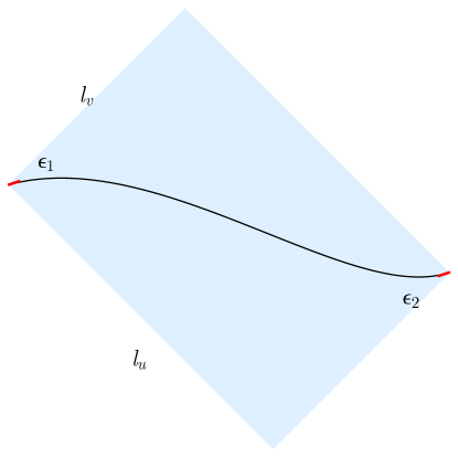
Figure 5: An arbitrary spacelike curve with a boosted DOD. The small red lines are the truncations $\epsilon_{1}$ and $\epsilon_{2}$ at the endpoints of the curve.

The most general case is that the two truncations have a boost relative to the examined DOD, as shown in Fig. 5. Consider an arbitrary spacelike curve, whose shape and size of the DOD are characterized by $l_{u}$ and $l_{v}$, and $\epsilon_{1}$, $\epsilon_{2}$ are cutoffs. Assume that

$$l_{u}l_{v}=(2R)^{2},\qquad\frac{l_{u}}{l_{v}}=e^{-2\kappa},\qquad\epsilon_{1}^{2}=\epsilon_{u1}\epsilon_{u2},\qquad\epsilon_{2}^{2}=\epsilon_{u2}\epsilon_{v2},$$ (64)

where

$$\frac{\epsilon_{u1}}{\epsilon_{v1}}=e^{-2\kappa_{1}},\qquad\frac{\epsilon_{u2}}{\epsilon_{v2}}=e^{-2\kappa_{2}}.$$ (65)

According to (63), we have

$$S=\frac{c_{L}+c_{R}}{12}\log\frac{(2R)^{2}}{\epsilon_{1}\epsilon_{2}}+\frac{c_{L}-c_{R}}{12}\left(\kappa_{1}+\kappa_{2}-2\kappa\right).$$ (66)

furthermore, we can set

$$\delta\kappa_{1}=\kappa_{1}-\kappa,\qquad\delta\kappa_{2}=\kappa_{2}-\kappa,$$ (67)

which are the boost angles of the cutoffs relative to the DOD. This means that when the total boost angle relative to the DOD vanishes, the anomalous contribution disappears. Otherwise, anomalous contributions will contribute, which have been discussed in some previous literatures Castro:2014tta ; Wall:2011kb ; Iqbal:2015vka .

4 Entanglement entropy from gravity

4.1 Rindler transformation in the bulk and Rindler AdS spacetime

In the rest of the article, for convenience, we always take $\beta_{u^{\prime}}=-\beta_{v^{\prime}}=\pi$, which will not affect the results. According to the Rindler method, in the bulk we have

$$\partial_{u^{\prime}} = a_{0}\tilde{L}_{0}+a_{+}\tilde{L}_{+}+a_{-}\tilde{L}_{-}=-\frac{l_{u}}{2}\tilde{L}_{+}+\frac{2}{l_{u}}\tilde{L}_{-}$$ (68)

$$= \left(\frac{l_{u}}{2}-\frac{2}{l_{u}}u^{2}\right)\partial_{u}+\frac{2}{l_{u}}z^{2}\partial_{v}-\frac{2}{l_{u}}uz\partial_{z},$$

$$\partial_{v^{\prime}} = b_{0}\tilde{\bar{L}}_{0}+b_{+}\tilde{\bar{L}}_{+}+b_{-}\tilde{\bar{L}}_{-}$$ (69)

$$= \frac{2}{l_{v}}z^{2}\partial_{u}+\left(\frac{l_{v}}{2}-\frac{2}{l_{v}}v^{2}\right)\partial_{v}-\frac{2}{l_{v}}vz\partial_{z}.$$

These two equations were obtained by directly replacing $l_{i}$ in (138) and (146) with $L_{i}$ and replace $\bar{l}_{i}$ with $\bar{L}_{i}$. After the Rindler transformation in the bulk, we can get the metric components from the AdS spacetime (22) as

$$g_{u^{\prime}u^{\prime}} = g_{ab}\left(\frac{\partial}{\partial u^{\prime}}\right)^{a}\left(\frac{\partial}{\partial u^{\prime}}\right)^{b}=1,\qquad g_{v^{\prime}v^{\prime}}=g_{ab}\left(\frac{\partial}{\partial v^{\prime}}\right)^{a}\left(\frac{\partial}{\partial v^{\prime}}\right)^{b}=1,$$ (70)

$$g_{u^{\prime}v^{\prime}} = g_{v^{\prime}u^{\prime}}=g_{ab}\left(\frac{\partial}{\partial u^{\prime}}\right)^{a}\left(\frac{\partial}{\partial v^{\prime}}\right)^{b}=\frac{l_{u}^{2}\left(l_{v}^{2}-4v^{2}\right)+4\left(-l_{v}^{2}u^{2}+4\left(uv+z^{2}\right)^{2}\right)}{8l_{u}l_{v}z^{2}}.$$ (71)

Since $\partial_{u^{\prime}}$ and $\partial_{v^{\prime}}$ are the Killing vector fields, the metric components should be independent of $u^{\prime},v^{\prime}$. We assume that $g_{u^{\prime}v^{\prime}}=F(z^{\prime})$ in which $F(z^{\prime})$ has good enough properties so that we can perform the following operations,

$$z^{\prime}=F^{-1}(g_{u^{\prime}v^{\prime}})$$ (72)

and

$$\left(dz^{\prime}\right)^{a} = \frac{-l_{v}^{2}u+4v\left(uv+z^{2}\right)}{l_{u}l_{v}z^{2}F^{\prime}\left(z^{\prime}\right)}\left(du\right)^{a}+\frac{-l_{u}^{2}v+4u\left(uv+z^{2}\right)}{l_{u}l_{v}z^{2}F^{\prime}\left(z^{\prime}\right)}\left(dv\right)^{a}$$ (73)

$$+\frac{-\left(l_{u}^{2}-4u^{2}\right)\left(l_{v}^{2}-4v^{2}\right)+16z^{4}}{4l_{u}l_{v}z^{3}F^{\prime}\left(z^{\prime}\right)}\left(dz\right)^{a},$$

where $F^{\prime}\left(z^{\prime}\right)$ represents the derivative with respect to $z^{\prime}$. Then we have

$$g^{z^{\prime}z^{\prime}}=g^{ab}(dz^{\prime})_{a}(dz^{\prime})_{b}=\frac{4(F(z^{\prime})^{2}-1)}{F^{\prime}(z^{\prime})^{2}}.$$ (74)

It is worth noting that Rindler AdS is not unique and we expect that the metric component $g_{u^{\prime}z^{\prime}}=g_{v^{\prime}z^{\prime}}=0$. Therefore, we reach

$$g_{z^{\prime}z^{\prime}}=\frac{F^{\prime}(z^{\prime})^{2}}{4(F(z^{\prime})^{2}-1)},$$ (75)

and

$$\left(\frac{\partial}{\partial z^{\prime}}\right)^{a} = \frac{g^{ab}\left(dz^{\prime}\right)_{b}}{g^{z^{\prime}z^{\prime}}}$$ (76)

$$= \frac{32l_{u}l_{v}z^{4}\left(4u\left(uv+z^{2}\right)-l_{u}^{2}v\right)F^{\prime}\left(z^{\prime}\right)}{A}\left(du\right)^{a}+\frac{32l_{u}l_{v}z^{4}\left(4v\left(uv+z^{2}\right)-l_{v}^{2}u\right)F^{\prime}\left(z^{\prime}\right)}{A}\left(dv\right)^{a}$$

$$+\frac{{4l_{u}l_{v}z^{3}\left(16z^{4}-\left(\left(l_{u}^{2}-4u^{2}\right)\left(l_{v}^{2}-4v^{2}\right)\right)\right)}}{A}\left(dz\right)^{a},$$

where

$$A = \left(\left(l_{u}+2u\right)\left(l_{v}-2v\right)-4z^{2}\right)\left(\left(l_{u}-2u\right)\left(l_{v}+2v\right)-4z^{2}\right)\left(\left(l_{u}-2u\right)\left(l_{v}-2v\right)+4z^{2}\right)$$ (77)

$$\times\left(\left(l_{u}+2u\right)\left(l_{v}+2v\right)+4z^{2}\right)$$

The transformations of the basis fields between $(u^{\prime},v^{\prime},z^{\prime})$ and $(u,v,z)$ are as follows,

$$\left(\frac{\partial}{\partial u^{\prime}}\right)^{a} =\frac{\partial u}{\partial u^{\prime}}\left(\frac{\partial}{\partial u}\right)^{a}+\frac{\partial v}{\partial u^{\prime}}\left(\frac{\partial}{\partial v}\right)^{a}+\frac{\partial z}{\partial u^{\prime}}\left(\frac{\partial}{\partial z}\right)^{a},$$ (78)

$$\left(\frac{\partial}{\partial v^{\prime}}\right)^{a} =\frac{\partial u}{\partial v^{\prime}}\left(\frac{\partial}{\partial u}\right)^{a}+\frac{\partial v}{\partial v^{\prime}}\left(\frac{\partial}{\partial v}\right)^{a}+\frac{\partial z}{\partial v^{\prime}}\left(\frac{\partial}{\partial z}\right)^{a},$$

$$\left(\frac{\partial}{\partial z^{\prime}}\right)^{a} =\frac{\partial u}{\partial z^{\prime}}\left(\frac{\partial}{\partial u}\right)^{a}+\frac{\partial v}{\partial z^{\prime}}\left(\frac{\partial}{\partial v}\right)^{a}+\frac{\partial z}{\partial z^{\prime}}\left(\frac{\partial}{\partial z}\right)^{a}.$$

They are connected by the Jacobian matrix and the inverse of the Jacobian matrix is

$$J^{-1}=\left(\begin{matrix}\frac{\partial u^{\prime}}{\partial u}&\frac{\partial v^{\prime}}{\partial u}&\frac{\partial z^{\prime}}{\partial u}\\ \frac{\partial u^{\prime}}{\partial v}&\frac{\partial v^{\prime}}{\partial v}&\frac{\partial z^{\prime}}{\partial v}\\ \frac{\partial u^{\prime}}{\partial z}&\frac{\partial v^{\prime}}{\partial z}&\frac{\partial z^{\prime}}{\partial z}\\ \end{matrix}\right).$$ (79)

The explicit forms of the entries can be readily get, therefore, we do not intend to present them explicitly because the expressions are rather complicated. Note that after integrating $\frac{\partial u^{\prime}}{\partial z}$ with respect to $z$, we get

$$u^{\prime}\left(u,v,z\right)=\int{\frac{\partial u^{\prime}}{\partial z}dz}+C\left(u,v\right),$$ (80)

where $C(u,v)$ is a function of $u,v$. As $z\rightarrow 0$, the Rindler transformation in the bulk should be the same as the Rindler transformation on the boundary, from which we can determine $C(u,v)$ and thus obtain $u^{\prime}(u,v,z)$. $v^{\prime}(u,v,z)$ can be obtained in the same way, and the final results are

$$u^{\prime}=\frac{1}{4}\log\frac{l_{v}^{2}\left(l_{u}+2u\right)^{2}-4\left(l_{u}v+2\left(uv+z^{2}\right)\right)^{2}}{l_{v}^{2}\left(l_{u}-2u\right)^{2}-4\left(l_{u}v-2\left(uv+z^{2}\right)\right)^{2}},$$ (81)

$$v^{\prime}=\frac{1}{4}\log\frac{l_{u}^{2}\left(l_{v}+2v\right)^{2}-4\left(l_{v}u+2\left(uv+z^{2}\right)\right)^{2}}{l_{u}^{2}\left(l_{v}-2v\right)^{2}-4\left(l_{v}u-2\left(uv+z^{2}\right)\right)^{2}}.$$ (82)

The three equations (72), (81), and (82) together constitute the Rindler transformation in the bulk. Under this transformation, the Rindler AdS metric has the following form

$$ds^{2}=du^{\prime 2}+dv^{\prime 2}+2F\left(z^{\prime}\right)du^{\prime}dv^{\prime}+\frac{F^{\prime}\left(z^{\prime}\right)^{2}}{4\left(F\left(z^{\prime}\right)^{2}-1\right)}dz^{\prime 2}.$$ (83)

It is easy to see that equations (81) and (82) are independent of the choice of $z^{\prime}$ (at least when $g_{u^{\prime}z^{\prime}}=g_{v^{\prime}z^{\prime}}=0$), and the first two columns of matrix $J^{-1}$ are also independent of the choice of $z^{\prime}$.

The radius of the horizon in Rindler AdS is

$$z^{\prime}_{h}=F^{-1}(1).$$ (84)

In order to obtain the thermal circle of Rindler AdS, we can expand the metric (83) near the horizon hartman2015lectures . Let $z^{\prime}=z^{\prime}_{h}(1+\epsilon^{2})$, as $\epsilon\rightarrow 0$ we have

$$ds^{2}\approx\frac{1}{2}F^{-1}\left(1\right)F^{\prime}\left(F^{-1}\left(1\right)\right)d\epsilon^{2}+\left(du^{\prime}+dv^{\prime}\right)^{2}+2F^{-1}\left(1\right)F^{\prime}\left(F^{-1}\left(1\right)\right)\epsilon^{2}du^{\prime}dv^{\prime}.$$ (85)

Now define a new coordinate $\phi=u^{\prime}+v^{\prime}$. If $\phi$ remains unchanged, that is, $d\phi=0$, then

$$ds^{2} \approx\frac{1}{2}F^{-1}\left(1\right)F^{\prime}\left(F^{-1}\left(1\right)\right)d\epsilon^{2}+\left({du^{\prime}+dv^{\prime}}\right)^{2}+2F^{-1}\left(1\right)F^{\prime}\left(F^{-1}\left(1\right)\right)\epsilon^{2}du^{\prime}dv^{\prime}$$ (86)

$$=\frac{1}{2}F^{-1}\left(1\right)F^{\prime}\left(F^{-1}\left(1\right)\right)d\epsilon^{2}-2F^{-1}\left(1\right)F^{\prime}\left(F^{-1}\left(1\right)\right)\epsilon^{2}du^{\prime 2}$$

$$=\frac{1}{2}F^{-1}\left(1\right)F^{\prime}\left(F^{-1}\left(1\right)\right)\left(d\epsilon^{2}-\epsilon^{2}\left(d\left(2u^{\prime}\right)\right)^{2}\right).$$

Therefore, the thermal circle is

$$\left(u^{\prime},v^{\prime}\right)\sim\left(u^{\prime}+i\pi,v^{\prime}-i\pi\right),$$ (87)

which is consistent with the results in the field theory.

In addition, we can also calculate the Killing vector fields of Rindler AdS spacetime. For $F(z^{\prime})>1$, the Killing vector fields are

$$\xi_{1} = \partial_{u^{\prime}},$$ (88)

$$\xi_{2} = \partial_{v^{\prime}},$$ (89)

$$\xi_{3} = -\frac{e^{2v^{\prime}}}{\sqrt{F\left(z^{\prime}\right)^{2}-1}}\partial_{u^{\prime}}+\frac{F\left(z^{\prime}\right)e^{2v^{\prime}}}{\sqrt{F\left(z^{\prime}\right)^{2}-1}}\partial_{v^{\prime}}-\frac{2\sqrt{F\left(z^{\prime}\right)^{2}-1}e^{2v^{\prime}}}{F^{\prime}\left(z^{\prime}\right)}\partial_{z^{\prime}},$$ (90)

$$\xi_{4} = -\frac{e^{-2v^{\prime}}}{\sqrt{F\left(z^{\prime}\right)^{2}-1}}\partial_{u^{\prime}}+\frac{F\left(z^{\prime}\right)e^{-2v^{\prime}}}{\sqrt{F\left(z^{\prime}\right)^{2}-1}}\partial_{v^{\prime}}+\frac{2\sqrt{F\left(z^{\prime}\right)^{2}-1}e^{-2v^{\prime}}}{F^{\prime}\left(z^{\prime}\right)}\partial_{z^{\prime}},$$ (91)

$$\xi_{5} = \frac{F\left(z^{\prime}\right)e^{2u^{\prime}}}{\sqrt{F\left(z^{\prime}\right)^{2}-1}}\partial_{u^{\prime}}-\frac{e^{2u^{\prime}}}{\sqrt{F\left(z^{\prime}\right)^{2}-1}}\partial_{v^{\prime}}-\frac{2e^{2u^{\prime}}\sqrt{F\left(z^{\prime}\right)^{2}-1}}{F^{\prime}\left(z^{\prime}\right)}\partial_{z^{\prime}},$$ (92)

$$\xi_{6} = \frac{F\left(z^{\prime}\right)e^{-2u^{\prime}}}{\sqrt{F\left(z^{\prime}\right)^{2}-1}}\partial_{u^{\prime}}-\frac{e^{-2u^{\prime}}}{\sqrt{F\left(z^{\prime}\right)^{2}-1}}\partial_{v^{\prime}}+\frac{2e^{-2u^{\prime}}\sqrt{F\left(z^{\prime}\right)^{2}-1}}{F^{\prime}\left(z^{\prime}\right)}\partial_{z^{\prime}}.$$ (93)

4.2 The thermal entropy of Rindler AdS

According to the Rindler method, the entanglement entropy in the field theory should be equal to the thermal entropy of Rindler AdS. Therefore, in this subsection, we will compute the black hole thermal entropy in TMG. The action contains the Einstein-Hilbert term, the cosmological constant term, and the Chern-Simons term

$$\mathcal{S}_{\mathrm{TMG}}=\frac{1}{16\pi G}\int{d^{3}}x\sqrt{-g}\left[R+2+\frac{1}{2\mu}\varepsilon^{\alpha\beta\gamma}\left({\Gamma^{\rho}}_{\alpha\sigma}\partial_{\beta}{\Gamma^{\sigma}}_{\alpha\rho}+\frac{2}{3}{\Gamma^{\rho}}_{\alpha\sigma}{\Gamma^{\sigma}}_{\beta\eta}{\Gamma^{\eta}}_{\gamma\rho}\right)\right].$$ (94)

where $\mu$ is a real coupling constant. The central charge of the dual CFT Kraus:2005zm is

$$c_{L}=\frac{3}{2G}\left(1+\frac{1}{\mu}\right),\qquad c_{R}=\frac{3}{2G}\left(1-\frac{1}{\mu}\right).$$ (95)

We can directly calculate the thermal entropy, and the contribution of the Chern-Simons term to the thermal entropy Jiang:2017ecm ; Tachikawa:2006sz is

$$S_{\text{CS}}=\frac{1}{4G\mu}\int_{\Sigma}\Gamma_{N},\qquad\Gamma_{N}=-\frac{1}{2}{\epsilon^{\mu}}_{\sigma}{\Gamma^{\sigma}}_{\mu\rho}dx^{\rho},$$ (96)

where $\Sigma$ is the surface $z^{\prime}=z^{\prime}_{h}$, where $z^{\prime}_{h}$ is the horizon radius. The nonvanishing connection coefficients can be obtained from the metric (83) as

$${\Gamma^{u^{\prime}}}_{u^{\prime}z^{\prime}} = {\Gamma^{u^{\prime}}}_{z^{\prime}u^{\prime}}=\frac{F\left(z^{\prime}\right)F^{\prime}\left(z^{\prime}\right)}{2\left(F\left(z^{\prime}\right)^{2}-1\right)},\qquad{\Gamma^{u^{\prime}}}_{v^{\prime}z^{\prime}}={\Gamma^{u^{\prime}}}_{z^{\prime}v^{\prime}}=\frac{F^{\prime}\left(z^{\prime}\right)}{2-2F\left(z^{\prime}\right)^{2}},$$ (97)

$${\Gamma^{v^{\prime}}}_{u^{\prime}z^{\prime}} = {\Gamma^{v^{\prime}}}_{z^{\prime}u^{\prime}}=\frac{F^{\prime}\left(z^{\prime}\right)}{2-2F\left(z^{\prime}\right)^{2}},\qquad{\Gamma^{v^{\prime}}}_{v^{\prime}z^{\prime}}={{\Gamma^{v^{\prime}}}_{z^{\prime}v^{\prime}}}=\frac{F\left(z^{\prime}\right)F^{\prime}\left(z^{\prime}\right)}{2\left(F\left(z^{\prime}\right)^{2}-1\right)},$$ (98)

$${\Gamma^{z^{\prime}}}_{u^{\prime}v^{\prime}} = {\Gamma^{z^{\prime}}}_{v^{\prime}u^{\prime}}=\frac{2-2F\left(z^{\prime}\right)^{2}}{F^{\prime}\left(z^{\prime}\right)},\qquad{\Gamma^{z^{\prime}}}_{z^{\prime}z^{\prime}}=\frac{F\left(z^{\prime}\right)F^{\prime}\left(z^{\prime}\right)}{1-F\left(z^{\prime}\right)^{2}}+\frac{F^{\prime\prime}\left(z^{\prime}\right)}{F^{\prime}\left(z^{\prime}\right)}.$$ (99)

From (88)-(93), we know that the Killing vector field orthogonal to $\Sigma$ is

$$\xi=\partial_{u^{\prime}}-\partial_{v^{\prime}}.$$ (100)

The binormal vector $\epsilon_{ab}$ on $\Sigma$ satisfies

$$k\epsilon_{ab}|_{\Sigma}=\nabla_{a}\xi_{b}|_{\Sigma},$$ (101)

where $k$ is a constant. Since the binormal vectors should also satisfy

$$\epsilon_{ab}\epsilon^{ab}=-2,$$ (102)

we take $k$ as

$$k=-\left.\sqrt{-\frac{1}{2}\nabla_{a}\xi_{b}\nabla^{a}\xi^{b}}\right|_{\varSigma}=-2.$$ (103)

Then we get

$$S_{\text{CS}}=\frac{\Delta u^{\prime}-\Delta v^{\prime}}{4G\mu}.$$ (104)

For our regularized intervals (37),

$$\Delta u^{\prime}=\frac{1}{2}\log\frac{l_{u}^{2}}{\varepsilon_{u1}\varepsilon_{u2}},\qquad\Delta v^{\prime}=\frac{1}{2}\log\frac{l_{v}^{2}}{\varepsilon_{v1}\varepsilon_{v2}}.$$ (105)

The total thermal entropy of Rindler AdS spacetime is

$$S_{\mathrm{Rindler}} =S_{BH}+S_{CS}$$ (106)

$$=\frac{\Delta u^{\prime}+\Delta v^{\prime}}{4G}+\frac{\Delta u^{\prime}-\Delta v^{\prime}}{4G\mu},$$

where $S_{BH}$ is the Bekenstein-Hawking entropy. Notice that

$$\frac{1}{4G}=\frac{c_{L}+c_{R}}{12},\qquad\frac{1}{4G\mu}=\frac{c_{L}-c_{R}}{12}$$ (107)

and

$$\Delta u^{\prime}+\Delta v^{\prime}=\frac{1}{2}\log\frac{l_{u}^{2}l_{v}^{2}}{\varepsilon_{u1}\varepsilon_{u2}\varepsilon_{v1}\varepsilon_{v2}},\qquad\Delta u^{\prime}-\Delta v^{\prime}=\frac{1}{2}\log\frac{l_{u}^{2}\varepsilon_{v1}\varepsilon_{v2}}{l_{v}^{2}\varepsilon_{u1}\varepsilon_{u2}},$$ (108)

then we get,

$$S_{\mathrm{Rindler}}=\frac{c_{L}+c_{R}}{24}\log\frac{l_{u}^{2}l_{v}^{2}}{\varepsilon_{u1}\varepsilon_{v1}\varepsilon_{u2}\varepsilon_{v2}}+\frac{c_{L}-c_{R}}{24}\log\frac{l_{u}^{2}\varepsilon_{v1}\varepsilon_{v2}}{l_{v}^{2}\varepsilon_{u1}\varepsilon_{u2}}.$$ (109)

Therefore, the entropy of Rindler AdS spacetime is consistent with the calculation of entanglement entropy in field theory (63). Moreover, the contribution of the Chern-Simons term to the black hole thermal entropy comes from the last term in the equation (109)

$$S_{CS}=\frac{c_{L}-c_{R}}{24}\log\frac{l_{u}^{2}\varepsilon_{v1}\varepsilon_{v2}}{l_{v}^{2}\varepsilon_{u1}\varepsilon_{u2}},$$ (110)

which is exactly the anomaly contribution in the field theory.

5 Entanglement entropy of zero temperature CFT on a cylinder and finite temperature CFT in a plane

It is well-known that the constraint equation (10) can be reformulated by the following coordinates  Aharony:1999ti ; Hartman:2013qma

$$\begin{cases}y_{0}=\cosh\rho\cos\tau,\\ y_{1}=\cosh\rho\sin\tau,\\ y_{2}=\sinh\rho\sin\theta,\\ y_{3}=-\sinh\rho\cos\theta,\\ \end{cases}$$ (111)

Here we have set the radius of AdS to be $L=1$. Therefore, the metric of AdS becomes

$$ds^{2}=-\cosh^{2}\rho d\tau^{2}+d\rho^{2}+\sinh\rho^{2}d\theta^{2}.$$ (112)

Its boundary is a cylinder with $\rho=\infty$. On the other hand, according to Eqs. (20) and (21), we know that to write AdS₃ in Poincaré coordinates, we have

$$\begin{cases}y_{0}=\frac{1-t^{2}+x^{2}+z^{2}}{2z},\\ y_{1}=\frac{t}{z},\\ y_{2}=\frac{x}{z},\\ y_{3}=\frac{-1-t^{2}+x^{2}+z^{2}}{2z}.\end{cases}$$ (113)

Therefore, the relationship between the global coordinates and the Poincaré coordinates is

$$\left\{\begin{array}[]{cc}t&=\frac{\cosh\rho\sin\tau}{\cos\tau\cosh\rho+\cos\theta\sinh\rho},\\ x&=\frac{\sin\theta\sinh\rho}{\cosh\rho\cos\tau+\sinh\rho\cos\theta},\\ z&=\frac{1}{\cosh\rho\cos\tau+\sinh\rho\cos\theta}.\end{array}\right.$$ (114)

On the boundary $\rho\to\infty$, this is precisely a conformal transformation,

$$\left\{\begin{array}[]{c}t=\frac{\sin\tau}{\cos\tau+\cos\theta},\\ x=\frac{\sin\theta}{\cos\tau+\cos\theta}.\\ \end{array}\right.$$ (115)

One can rewrite it in the form of light-like coordinates as

$$\left\{\begin{array}[]{c}u=\tan\frac{U}{2},\\ v=\tan\frac{V}{2}.\end{array}\right.$$ (116)

where $U=\theta+\tau$, $V=\theta-\tau$, are exactly the transformations between the plane and the Lorentzian cylinder in two-dimensional Minkowski spacetime Mack:1988nf . In principle, (116) together with (32) and (33) can give a Rindler transformation that maps a zero-temperature CFT on a cylinder to a finite-temperature CFT on a plane. Consider an interval on the cylinder (the upper label of $\mathcal{I}^{c}$ represents cylinder)

$$\mathcal{I}^{c}\equiv\left\{\left(U,V\right)\bigg{|}U=l_{U}\left(s-\frac{1}{2}\right),V=l_{V}\left(s-\frac{1}{2}\right),s\in\left[0,1\right]\right\}$$ (117)

Under the transformations, it becomes an interval on the plane,

$$\mathcal{I}^{p}\equiv\left\{\left(u,v\right)\bigg{|}u=\tan\left[\frac{l_{U}}{2}\left(s-\frac{1}{2}\right)\right],v=\tan\left[\frac{l_{V}}{2}\left(s-\frac{1}{2}\right)\right],s\in\left[0,1\right]\right\}$$ (118)

Thus, computing the entanglement entropy of $\mathcal{I}^{p}$ on the plane can obtain the entanglement entropy of the interval $\mathcal{I}^{c}$. Considering the entanglement entropy formula (62), as well as the length of the interval and the UV cutoff, we can obtain the entanglement entropy. The length of interval $\mathcal{I}^{p}$ are

$$l_{u}^{p}=2\tan\frac{l_{U}}{4},\qquad l_{v}^{p}=2\tan\frac{l_{V}}{4}.$$ (119)

If we assume that the regulated interval on the cylinder is

$$\mathcal{I}^{\prime c}\equiv\left\{\left(U,V\right)\bigg{|}U=l_{U}\left(s-\frac{1}{2}\right),V=l_{V}\left(s-\frac{1}{2}\right),s\in\left[\varepsilon_{1},1-\varepsilon_{2}\right]\right\}$$ (120)

and let

$$\varepsilon_{U1}=l_{U}\varepsilon_{1},\qquad\varepsilon_{U2}=l_{U}\varepsilon_{2},$$ (121)

$$\varepsilon_{V1}=l_{V}\varepsilon_{1},\qquad\varepsilon_{V2}=l_{V}\varepsilon_{2},$$ (122)

the regulated interval can be readily obtained after the conformal transformation (116),

$${\mathcal{I}^{\prime}}^{p}\equiv\left\{\left(u,v\right)\bigg{|}u=\tan\left[\frac{l_{U}}{2}\left(s-\frac{1}{2}\right)\right],v=\tan\left[\frac{l_{V}}{2}\left(s-\frac{1}{2}\right)\right],s\in\left[\varepsilon_{1},1-\varepsilon_{2}\right]\right\}$$ (123)

The cutoffs can be read from the regulated interval $\mathcal{I}^{\prime p}$ as

$$\varepsilon_{u1}^{p}\equiv\tan\left(\frac{1}{2}\varepsilon_{U1}-\frac{l_{U}}{4}\right)-\tan\left(-\frac{l_{U}}{4}\right),\qquad\varepsilon_{u2}^{p}\equiv\tan\frac{l_{U}}{4}-\tan\left(\frac{l_{U}}{4}-\frac{1}{2}\varepsilon_{U2}\right),$$ (124)

$$\varepsilon_{v1}^{p}\equiv\tan\left(\frac{1}{2}\varepsilon_{V1}-\frac{l_{V}}{4}\right)-\tan\left(-\frac{l_{V}}{4}\right),\qquad\varepsilon_{v2}^{p}\equiv\tan\frac{l_{V}}{4}-\tan\left(\frac{l_{V}}{4}-\frac{1}{2}\varepsilon_{V2}\right).$$ (125)

Substituting them into Eq. (62), one can obtain the entanglement entropy on the cylinder

$$S =\frac{c_{L}}{12}\log\frac{\left(l_{u}^{p}\right)^{2}}{\varepsilon_{u1}^{p}\varepsilon_{u2}^{p}}+\frac{c_{R}}{12}\log\frac{\left(l_{v}^{p}\right)^{2}}{\varepsilon_{v1}^{p}\varepsilon_{v2}^{p}}$$ (126)

$$=\frac{c_{L}}{12}\log\frac{\left(2\tan\frac{l_{U}}{4}\right)^{2}}{\left(\tan\left(\frac{1}{2}\varepsilon_{U1}-\frac{l_{U}}{4}\right)-\tan\left(-\frac{l_{U}}{4}\right)\right)\left(\tan\frac{l_{U}}{4}-\tan\left(\frac{l_{U}}{4}-\frac{1}{2}\varepsilon_{U2}\right)\right)}$$

$$+\frac{c_{R}}{12}\log\frac{\left(2\tan\frac{l_{V}}{4}\right)^{2}}{\left(\tan\left(\frac{1}{2}\varepsilon_{V1}-\frac{l_{V}}{4}\right)-\tan\left(-\frac{l_{V}}{4}\right)\right)\left(\tan\frac{l_{V}}{4}-\tan\left(\frac{l_{V}}{4}-\frac{1}{2}\varepsilon_{V2}\right)\right)}$$

$$\approx\frac{c_{L}}{12}\log\frac{4\sin^{2}\frac{l_{U}}{2}}{\varepsilon_{U1}\varepsilon_{U2}}+\frac{c_{R}}{12}\frac{4\sin^{2}\frac{l_{V}}{2}}{\varepsilon_{V1}\varepsilon_{V2}}$$

$$=\frac{c_{L}+c_{R}}{24}\log\frac{16\sin^{2}\frac{l_{U}}{2}\sin^{2}\frac{l_{V}}{2}}{\varepsilon_{U1}\varepsilon_{V1}\varepsilon_{U2}\varepsilon_{V2}}+\frac{c_{L}-c_{R}}{24}\log\frac{\sin^{2}\frac{l_{U}}{2}\varepsilon_{V1}\varepsilon_{V2}}{\sin^{2}\frac{l_{V}}{2}\varepsilon_{U1}\varepsilon_{U2}},$$

in which the last term is the contribution of the Chern-Simons term to the black hole entropy in the bulk

$$S_{CS}=\frac{c_{L}-c_{R}}{24}\log\frac{\sin^{2}\frac{l_{U}}{2}\varepsilon_{V1}\varepsilon_{V2}}{\sin^{2}\frac{l_{V}}{2}\varepsilon_{U1}\varepsilon_{U2}}.$$ (127)

As in the previous discussion, these cutoffs do not generally need to satisfy equations (121) and (122). It is worth noting that the results we have obtained are for CFT with a spatial circle

$$U\sim U+2\pi,\qquad V\sim V+2\pi.$$ (128)

If we consider a CFT with an arbitrary spatial circle

$$U\sim U+L_{U},\qquad V\sim V+L_{V},$$ (129)

we need to make the following substitution in (126) and (127),

$$l_{U}\rightarrow\frac{l_{U}}{L_{U}/2\pi},\qquad l_{V}\rightarrow\frac{l_{V}}{L_{V}/2\pi},$$ (130)

$$\varepsilon_{U1}\rightarrow\frac{\varepsilon_{U1}}{L_{U}/2\pi},\qquad\varepsilon_{V1}\rightarrow\frac{\varepsilon_{V1}}{L_{V}/2\pi},$$ (131)

$$\varepsilon_{U2}\rightarrow\frac{\varepsilon_{U2}}{L_{U}/2\pi},\qquad\varepsilon_{V2}\rightarrow\frac{\varepsilon_{V2}}{L_{V}/2\pi}.$$ (132)

Ultimately, we obtain

$$S=\frac{c_{L}+c_{R}}{24}\log\frac{L_{U}^{2}L_{V}^{2}\sin^{2}\frac{\pi l_{U}}{L_{U}}\sin^{2}\frac{\pi l_{V}}{L_{V}}}{\pi^{4}\varepsilon_{U1}\varepsilon_{V1}\varepsilon_{U2}\varepsilon_{V2}}+\frac{c_{L}-c_{R}}{24}\log\frac{L_{U}^{2}\sin^{2}\frac{\pi l_{U}}{L_{U}}\varepsilon_{V1}\varepsilon_{V2}}{L_{V}^{2}\sin^{2}\frac{\pi l_{V}}{L_{V}}\varepsilon_{U1}\varepsilon_{U2}},$$ (133)

and the contribution from the Chern-Simons term is

$$S_{CS}=\frac{c_{L}-c_{R}}{24}\log\frac{L_{U}^{2}\sin^{2}\frac{\pi l_{U}}{L_{U}}\varepsilon_{V1}\varepsilon_{V2}}{L_{V}^{2}\sin^{2}\frac{\pi l_{V}}{L_{V}}\varepsilon_{U1}\varepsilon_{U2}}.$$ (134)

Based on these formulae, replacing the spatial circle with a thermal circle ($L_{U}\rightarrow i\beta_{U},L_{V}\rightarrow i\beta_{V}$) will directly yield the entanglement entropy of the finite-temperature CFT and the corrections of the Chern-Simons term to the thermal entropy in the bulk. They are,

$$S = \frac{c_{L}+c_{R}}{24}\log\frac{\beta_{U}^{2}\beta_{V}^{2}\sinh^{2}\frac{\pi l_{U}}{\beta_{U}}\sinh^{2}\frac{\pi l_{V}}{\beta_{V}}}{\pi^{4}\varepsilon_{U1}\varepsilon_{V1}\varepsilon_{U2}\varepsilon_{V2}}+\frac{c_{L}-c_{R}}{24}\log\frac{\beta_{U}^{2}\sinh^{2}\frac{\pi l_{U}}{\beta_{U}}\varepsilon_{V1}\varepsilon_{V2}}{\beta_{V}^{2}\sinh^{2}\frac{\pi l_{V}}{\beta_{V}}\varepsilon_{U1}\varepsilon_{U2}},$$ (135)

$$S_{CS} = \frac{c_{L}-c_{R}}{24}\log\frac{\beta_{U}^{2}\sinh^{2}\frac{\pi l_{U}}{\beta_{U}}\varepsilon_{V1}\varepsilon_{V2}}{\beta_{V}^{2}\sinh^{2}\frac{\pi l_{V}}{\beta_{V}}\varepsilon_{U1}\varepsilon_{U2}}.$$ (136)

It is obvious that if we take $c_{L}=c_{R}$ and choose the subsystem to be an interval on the equal-time surface, our previous results can all return to the results of the two-dimensional conformal field theory Calabrese:2004eu ; Calabrese:2009qy . For $c_{L}\neq c_{R}$, equations (133) and (135) do not necessarily have anomalous contributions, for example, there are no anomalous contributions when

$$\begin{array}[]{c}L_{U}^{2}\sin^{2}\frac{\pi l_{U}}{L_{U}}\varepsilon_{V1}\varepsilon_{V2}=L_{V}^{2}\sin^{2}\frac{\pi l_{V}}{L_{V}}\varepsilon_{U1}\varepsilon_{U2},\\ \beta_{U}^{2}\sinh^{2}\frac{\pi l_{U}}{\beta_{U}}\varepsilon_{V1}\varepsilon_{V2}=\beta_{V}^{2}\sinh^{2}\frac{\pi l_{V}}{\beta_{V}}\varepsilon_{U1}\varepsilon_{U2.}\end{array}$$ (137)

6 Conclusions

In this paper, we studied the entanglement entropy of the two-dimensional CFT with gravitational anomalies and derived some of their important properties. By reviewing AdS₃ spacetime and calculating Killing vector fields, we derived the global conformal transformation generators of the boundary CFT. Using the generalized Rindler method, we derived the Rindler transformation in two-dimensional planar CFT and calculated the entanglement entropy of CFT with gravitational anomalies in the field theory. In addition, we also derived the Rindler transformation in the bulk and found that the transformation of the $u,v$ coordinates in the bulk has nothing to do with the transformation of $z$ coordinate. From the relationship between global coordinates and Poincaré coordinates in the bulk, we derived the transformation between the plane and Lorentzian cylinder on the boundary and found that this transformation is consistent with that in Mack’s paper Mack:1988nf . Finally, using conformal transformations, we calculated the entanglement entropy of CFT on a plane and derived the entanglement entropy formula for zero-temperature CFT on a cylinder and the entanglement entropy of CFT with temperature on a plane. We found that the entanglement entropy we calculated in field theory is indeed equal to the black hole entropy in Rindler AdS. Specifically, for a zero-temperature CFT on a plane, if the total boost angle ($\delta\kappa_{1}+\delta\kappa_{2}$) of the cutoffs relative to the space-like diagonal of the DOD of the subregion is not zero, then there will be an anomalous contribution to the entanglement entropy. These results are important for further understandings of the two-dimensional CFT with gravitational anomalies and may deepen our understanding of holographic entanglement entropy.

Appendix A Derive the Rindler transformation

Considering only $u^{\prime}=f(u)$, we can obtain from equations (25) and (28):

$$\partial_{u^{\prime}} =\frac{du}{du^{\prime}}\partial_{u}=a_{0}l_{0}+a_{+}l_{+}+a_{-}l_{-}=\left(a_{0}u-a_{+}-u^{2}a_{-}\right)\partial_{u}.$$ (138)

This implies that we only need to solve

$$\frac{du^{\prime}}{du}=\frac{1}{a_{0}u-a_{+}-u^{2}a_{-}}$$ (139)

to obtain the Rindler transformation up to some undetermined constants $c$. One can easily get

$$u^{\prime}=-\frac{2\arctan\frac{2a_{-}u-a_{0}}{\sqrt{4a_{+}a_{-}-a^{2}_{0}}}}{\sqrt{4a_{+}a_{-}-a^{2}_{0}}}+c$$ (140)

and then solve for $u$ as

$$u=\frac{a_{0}-\sqrt{4a_{+}a_{-}-a_{0}^{2}}}{2a_{-}}\tan\left(\frac{1}{2}\sqrt{4a_{+}a_{-}-a_{0}^{2}}u^{\prime}\right).$$ (141)

Here, without loss of generality, we have taken the constant $c$ to be $0$. It is easy to see that an imaginary periodicty exists in the $u^{\prime}$ direction only when $4a_{+}a_{-}-a^{2}_{0}<0$ is satisfied, and the imaginary periodicty is:

$$\beta_{u^{\prime}}=\frac{2\pi}{\sqrt{a^{2}_{0}-4a_{+}a_{-}}}.$$ (142)

The generator of the modular flow is given by $k_{t}=\beta_{u^{\prime}}(a_{0}u-a_{+}-u^{2}a_{-})\partial_{u}+\beta_{v^{\prime}}\frac{dv}{dv^{\prime}}\partial_{v}$. To ensure that the boundary of $\mathcal{I}$ remains invariant under $k_{t}$, we must have

$$a_{0}\frac{l_{u}}{2}-a_{+}-(l_{u}/2)^{2}a_{-} =0$$ (143)

$$-a_{0}\frac{l_{u}}{2}-a_{+}-(-l_{u}/2)^{2}a_{-} =0$$

From (142) and (143), we can obtain the following solution

$$\left\{\begin{array}[]{ccc}a_{0}&=&0,\\ a_{+}&=&-\frac{l_{u}\pi}{2\beta_{u^{\prime}}},\\ a_{-}&=&\frac{2\pi}{\beta_{u^{\prime}}l_{u}}.\\ \end{array}\right.$$ (144)

Therefore, the Rindler transformation can be determined as follows

$$u^{\prime}=\frac{\beta_{u^{\prime}}}{\pi}\arctan\!\text{h}\frac{2u}{l_{u}}.$$ (145)

Similarly, one can get

$$\partial_{v^{\prime}} =\frac{dv}{dv^{\prime}}\partial_{v}=b_{0}\bar{l}_{0}+b_{+}\bar{l}_{+}+b_{-}\bar{l}_{-}=\left(-b_{0}v+b_{+}v^{2}+b_{-}\right)\partial_{v},$$ (146)

By comparing equations (138) and (146), we can take

$$v^{\prime}=-\frac{\beta_{v^{\prime}}}{\pi}\arctan\!\text{h}\frac{2v}{l_{v}}$$ (147)

with the periodicity

$$v^{\prime}\sim v^{\prime}+i\beta_{v^{\prime}},\qquad\beta_{v^{\prime}}=\frac{2\pi}{b^{2}_{0}-4b_{+}b_{-}}.$$ (148)

The constants in equation (146) can be determined,

$$\left\{\begin{array}[]{ccc}b_{0}&=&0,\\ b_{+}&=&\frac{2\pi}{\beta_{v^{\prime}}l_{v}},\\ b_{-}&=&-\frac{l_{v}\pi}{2\beta_{v^{\prime}}}.\\ \end{array}\right.$$ (149)

Since $\beta_{u^{\prime}}$ and $\beta_{v^{\prime}}$ do not appear in the expression of entangled entropy, the choice of $\beta_{u^{\prime}}$ and $\beta_{v^{\prime}}$ is arbitrary.

- (1) Ryszard Horodecki, Paweł Horodecki, Michał Horodecki, and Karol Horodecki. Quantum entanglement. Rev. Mod. Phys., 81:865–942, Jun 2009.
- (2) Thomas Hartman. Lectures on quantum gravity and black holes. Cornell University, 2015.
- (3) Pasquale Calabrese and John L. Cardy. Entanglement entropy and quantum field theory. J. Stat. Mech., 0406:P06002, 2004.
- (4) Pasquale Calabrese and John Cardy. Entanglement entropy and conformal field theory. J. Phys. A, 42:504005, 2009.
- (5) Shinsei Ryu and Tadashi Takayanagi. Holographic derivation of entanglement entropy from AdS/CFT. Phys. Rev. Lett., 96:181602, 2006.
- (6) Shinsei Ryu and Tadashi Takayanagi. Aspects of Holographic Entanglement Entropy. JHEP, 08:045, 2006.
- (7) Veronika E. Hubeny, Mukund Rangamani, and Tadashi Takayanagi. A Covariant holographic entanglement entropy proposal. JHEP, 07:062, 2007.
- (8) Juan Martin Maldacena. The Large N limit of superconformal field theories and supergravity. Adv. Theor. Math. Phys., 2:231–252, 1998.
- (9) Edward Witten. Anti-de Sitter space and holography. Adv. Theor. Math. Phys., 2:253–291, 1998.
- (10) Dmitri V. Fursaev. Proof of the holographic formula for entanglement entropy. JHEP, 09:018, 2006.
- (11) Horacio Casini, Marina Huerta, and Robert C. Myers. Towards a derivation of holographic entanglement entropy. JHEP, 05:036, 2011.
- (12) Aitor Lewkowycz and Juan Maldacena. Generalized gravitational entropy. JHEP, 08:090, 2013.
- (13) Xi Dong, Aitor Lewkowycz, and Mukund Rangamani. Deriving covariant holographic entanglement. JHEP, 11:028, 2016.
- (14) Tatsuma Nishioka. Entanglement entropy: holography and renormalization group. Rev. Mod. Phys., 90(3):035007, 2018.
- (15) Mukund Rangamani and Tadashi Takayanagi. Holographic Entanglement Entropy, volume 931. Springer, 2017.
- (16) Alejandra Castro, Diego M. Hofman, and Nabil Iqbal. Entanglement Entropy in Warped Conformal Field Theories. JHEP, 02:033, 2016.
- (17) Wei Song, Qiang Wen, and Jianfei Xu. Modifications to Holographic Entanglement Entropy in Warped CFT. JHEP, 02:067, 2017.
- (18) Hongliang Jiang, Wei Song, and Qiang Wen. Entanglement Entropy in Flat Holography. JHEP, 07:142, 2017.
- (19) Hongliang Jiang. Anomalous Gravitation and its Positivity from Entanglement. JHEP, 10:283, 2019.
- (20) Alejandra Castro, Stephane Detournay, Nabil Iqbal, and Eric Perlmutter. Holographic entanglement entropy and gravitational anomalies. JHEP, 07:114, 2014.
- (21) Jia-Rui Sun. Note on Chern-Simons Term Correction to Holographic Entanglement Entropy. JHEP, 05:061, 2009.
- (22) Per Kraus and Finn Larsen. Holographic gravitational anomalies. JHEP, 01:022, 2006.
- (23) Esko Keski-Vakkuri. Bulk and boundary dynamics in BTZ black holes. Phys. Rev. D, 59:104001, Mar 1999.
- (24) Makoto Natsuume. AdS/CFT Duality User Guide, volume 903. 2015.
- (25) Qiang Wen. Fine structure in holographic entanglement and entanglement contour. Phys. Rev. D, 98(10):106004, 2018.
- (26) Ralph Blumenhagen and Erik Plauschinn. Introduction to conformal field theory: with applications to String theory, volume 779. 2009.
- (27) P. Di Francesco, P. Mathieu, and D. Senechal. Conformal Field Theory. Graduate Texts in Contemporary Physics. Springer-Verlag, New York, 1997.
- (28) John L. Cardy. Operator Content of Two-Dimensional Conformally Invariant Theories. Nucl. Phys. B, 270:186–204, 1986.
- (29) Thomas Hartman, Christoph A. Keller, and Bogdan Stoica. Universal Spectrum of 2d Conformal Field Theory in the Large c Limit. JHEP, 09:118, 2014.
- (30) Aron C. Wall. Testing the Generalized Second Law in 1+1 dimensional Conformal Vacua: An Argument for the Causal Horizon. Phys. Rev. D, 85:024015, 2012.
- (31) Nabil Iqbal and Aron C. Wall. Anomalies of the Entanglement Entropy in Chiral Theories. JHEP, 10:111, 2016.
- (32) Yuji Tachikawa. Black hole entropy in the presence of Chern-Simons terms. Class. Quant. Grav., 24:737–744, 2007.
- (33) Ofer Aharony, Steven S. Gubser, Juan Martin Maldacena, Hirosi Ooguri, and Yaron Oz. Large N field theories, string theory and gravity. Phys. Rept., 323:183–386, 2000.
- (34) Thomas Hartman and Juan Maldacena. Time Evolution of Entanglement Entropy from Black Hole Interiors. JHEP, 05:014, 2013.
- (35) G. Mack. INTRODUCTION TO CONFORMAL INVARIANT QUANTUM FIELD THEORY IN TWO-DIMENSIONS AND MORE DIMENSIONS. In NATO Advanced Summer Institute on Nonperturbative Quantum Field Theory (Cargese Summer Institute), 8 1988.