Finding Meaningful Distributions of ML Black-boxes
under Forensic Investigation

Abstract.

Given a poorly documented neural network model, we take the perspective of a forensic investigator who wants to find out the model’s data domain (e.g. whether on face images or traffic signs). Although existing methods such as membership inference and model inversion can be used to uncover some information about an unknown model, they still require knowledge of the data domain to start with. In this paper, we propose solving this problem by leveraging on comprehensive corpus such as ImageNet to select a meaningful distribution that is close to the original training distribution and leads to high performance in follow-up investigations. The corpus comprises two components, a large dataset of samples and meta information such as hierarchical structure and textual information on the samples. Our goal is to select a set of samples from the corpus for the given model. The core of our method is an objective function that considers two criteria on the selected samples: the model functional properties (derived from the dataset), and semantics (derived from the metadata). We also give an algorithm to efficiently search the large space of all possible subsets w.r.t. the objective function. Experimentation results show that the proposed method is effective. For example, cloning a given model (originally trained with CIFAR-10) by using Caltech 101 can achieve 45.5% accuracy. By using datasets selected by our method, the accuracy is improved to 72.0%.

1. Introduction

Machine learning models, in particular, deep neural networks have achieved excellent performance in many tasks. The development of easy-to-use training tools and widely available datasets further accelerate their adoption. While the wide adoption is encouraging, it would not be surprising to see involvement of ML models in illegal activities.

Here, we take the perspective of forensic investigators, who want to investigate some suspicious ML models and determine the purpose of the models. These ML models could be in the form of black-boxes and embedded in some apprehended devices with internal mechanisms hidden, for instance, the models are embedded in FPGA, ASIC, or Trusted Execution Environment such as Intel SGX (Schunter, 2016). They could also be in the form of remote services that receive and send inputs/predictions over the Internet.

Although we adopt a black-box threat model, in practice, in the white-box setting (where investigators can examine parameters and intermediate states), due to lack of transparency/explainability, limited information can be obtained. Therefore, such investigation is also applicable to poorly documented white-box models, for example, model files stored in Google Drive with format such as ‘.pth’ or ‘.ckpt’.

Methods such as membership inference (Jia et al., 2019; Rahman et al., 2018; Chen et al., 2020; Li and Zhang, 2020; Shokri et al., 2017; Salem et al., 2019), model cloning (Tramèr et al., 2016; Papernot et al., 2017; Oh et al., 2019; Wang and Gong, 2018; Lowd and Meek, 2005; Milli et al., 2019; Orekondy et al., 2019) and model inversion (Fredrikson et al., 2015; Lee and Kil, 1994; Lu et al., 1999; Mahendran and Vedaldi, 2015; Dosovitskiy and Brox, 2016b, a; Nash et al., 2019; Yang et al., 2019) can be deployed to provide useful information of an unknown model. However, most of these methods require some knowledge about the data domain of the model to start from, for instance, whether they are face images, X-ray images, etc. These methods either become ineffective or have decreased performance if such information is inaccurate.

In this paper, we work on a new task which fills in the above-mentioned gap by determining the data domain of model with black-box and hard-label only access. We do not aim to find the exact original data distribution nor the training set that the model was trained on. Instead, we are contended with some meaningful datasets that could lead to high performance from the follow-up investigation.

Due to the domain’s high dimensionality, there could be many drastically different training sets that lead to the target model. We leverage on comprehensive corpus gathered by the research community as a starting point, based on the assumption that the black-box models are trained on meaningful images with similar semantics captured in the corpus.

Problem Statement.  Given a black-box model and access to a comprehensive corpus, the investigator wants to find a candidate distribution which is close to the original training data distribution of the model.

A corpus contains a large dataset and metadata which links data points according to their semantics. The investigator wants to identify whether the corpus contains data points which are similar to the target model’s training data. Then the investigator extracts a subset from the corpus to form a candidate distribution as the outcome of the investigation.

In our approach, we use an objective function which is a weighted sum of two terms to find a good distribution. The first term focuses on the black-box model’s response to input data and covers the functional aspect of the target model. The second term makes use of the metadata, in particular, the hierarchical structure, to measure how semantically meaningful the candidate distribution is. As the search space is extremely large, We propose a heuristic to efficiently search for a good candidate distribution.

Experimentation results demonstrate that the proposed approach can effectively find candidate datasets that are close to the original input distribution and boost the performance of further investigations. For example, when conducting model cloning on a model originally trained on a subset of CIFAR-10 with a fixed small number of samples, using a similar dataset (Caltech101) can achieve 45.5% testing accuracy and using our selected dataset can achieve 72.0%. We also conducted experiments on two undocumented models downloaded from public domain. Using our method, we suspect that the first one is trained on ImageNet and classifies the 1,000 classes in ImageNet. For the second one, we suspect that it is trained on three classes of plants. Further analysis suggests that it may be trained on some leaves that look like bean leaves.

Contributions.

1. We highlight that determining an accurate input distribution of a given model is an important first step for machine learning forensic investigations.

2. We propose a method to find a dataset that is close to the training distribution of a given classifier. This method uses background information supplied by a hierarchical corpus. It has two main components: an objective function that evaluates whether a candidate dataset is good and an algorithm to search from all subsets of the corpus.

3. We evaluate the effectiveness of our approach under several settings: (a) Find the input data distribution for classifiers with known ground truth, (b) Find the input data distribution for unknown models hosted in model hubs, (c) Use the datasets obtained through the proposed method for follow-up investigation, in particular, model cloning.

2. Background and Related Works

The problem we are trying to solve is related but different from the goal of model inversion and membership inference. This section gives a brief overview of these two works. In addition, the main purpose of our method is to find a suitable dataset for follow-up investigations, such as model cloning. This section also includes an introduction to model cloning.

2.1. Model Inversion

Model inversion is a method which aims to extract information related to the input data of a model. Most model inversion approaches focus on reconstructing an input image from the soft predictions. In such cases, given a neural network classification model ${\mathcal{M}}:\mathcal{X}\rightarrow\mathbb{R}^{n}$ trained on a data distribution ${\mathcal{D}}$, the goal of model inversion is to create a model $\widehat{{\mathcal{M}}}:\mathbb{R}^{n}\rightarrow\mathcal{X}$ such that for x sampled from ${\mathcal{D}}$, the new model is able to reconstruct x from the target classifier’s output ${\mathcal{M}}({\textbf{x}})$, i.e. $\widehat{{\mathcal{M}}}({\mathcal{M}}({\textbf{x}}))={\textbf{x}}$.

Model inversion can be categorized into gradient-based methods (Fredrikson et al., 2015; Lee and Kil, 1994; Lu et al., 1999; Mahendran and Vedaldi, 2015) which invert a model using some optimization functions, and training-based methods (Dosovitskiy and Brox, 2016b, a; Nash et al., 2019; Yang et al., 2019) which learn new substitute models as the inverse of original target models. Both categories require access to soft predictions of the target models. Some methods also need white-box access to exploit backpropagation.

If only hard-label access is permitted, the problem can also be further reduced to class inversion which creates representative samples for each class. Though model inversion is able to reconstruct a single input or create representative samples for a class, background information about the training distribution is still required.

2.2. Membership Inference

Given a model $\mathcal{M}$ and a particular sample x, the purpose of membership inference is to find out whether this sample x is included in the training dataset $\mathcal{D}$ of the model $\mathcal{M}$. There are different versions of membership inference with different settings (Jia et al., 2019; Rahman et al., 2018; Chen et al., 2020; Li and Zhang, 2020; Shokri et al., 2017; Salem et al., 2019). Most existing works assume the investigator has some knowledge about the architecture of the target model. In addition, the investigator also needs some background about the distribution of the target model’s training dataset. Such background knowledge may be in the form of some samples from same distribution but not included in the training dataset.

2.3. Model Cloning

Given a black-box neural network classification model $\mathcal{M}:\mathcal{X}\rightarrow\mathbb{R}^{n}$ trained on a data distribution ${\mathcal{D}}$, the goal of model cloning is to create a model $\widetilde{\mathcal{M}}:\mathcal{X}\rightarrow\mathbb{R}^{n}$ such that for most x sampled from ${\mathcal{D}}$, the new model produces the same prediction result as the original target model, i.e. $\widetilde{\mathcal{M}}({\textbf{x}})=\operatorname*{arg\,max}\mathcal{M}({\textbf{x}})$.

There are extensive studies on model cloning. Tramer et al. proposed cloning single layer logistic regression models using equation solving method and cloning decision tree models using path finding method (Tramèr et al., 2016). Their methods do not require the usage of natural samples but assume that the investigator knows about architecture and training procedures of the target model. Soft predictions (a.k.a confidence scores) are also required. Papernot et al. demonstrated the effectiveness of model cloning on more complicated models (Papernot et al., 2017). Their method does not require the knowledge about target model’s architecture or training details. They use synthesized natural samples from the same distribution as the target model’s training data and applied a fixed training strategy for cloning. Only hard labels are required. Methods with similar goals were also explored in many other literatures (Oh et al., 2019; Wang and Gong, 2018; Lowd and Meek, 2005; Milli et al., 2019; Orekondy et al., 2019).

3. Problem Formulation

The investigator has hard-label black-box access to a model ${\mathcal{M}}$ with $n$ classes. That is, the investigators can adaptively submit inputs to the black-box, and receive the output in the form of one-hot vectors. For the given ${\mathcal{M}}$, let us write ${\mathcal{M}}({\bf x})$ as the array of soft labels of all classes on input ${\bf x}$ and ${\mathcal{M}_{i}}({\bf x})$ as the soft label for the $i$-th class on input ${\bf x}$.

The investigator also has a corpus $\mathcal{C}=\langle\mathcal{D},\mathcal{T}\rangle$, which consists of a dataset $\mathcal{D}$ and the associated metadata $\mathcal{T}$. For example, $\mathcal{D}$ is the set of images in ImageNet, and the metadata $\mathcal{T}$ contains the textual description of each class and describes the hierarchical relationship among the classes.

3.1. Output of Investigation

The investigator wants to select a set of samples from dataset $\mathcal{D}$. For each class $i$, we define $\omega_{i}$ as the set of indices of the selected samples. For example, if $\omega_{i}=\{i_{1},i_{2},...,i_{k}\}$, then $i_{1}\text{-th},i_{2}\text{-th},...,i_{k}\text{-th}$ samples in $\mathcal{D}$ are being selected. In addition, we denote the set of images with indices in $\omega^{\prime}$ as $\mathcal{D_{\omega^{\prime}}}$.

In summary, the output of the investigation is the set of selection parameters for $n$-classes, denoted as $\omega=\langle\omega_{1},\omega_{2},\ldots,\omega_{n}\rangle$.

The $n$-class dataset selected by the selection parameters is denoted as ${\mathcal{D}}_{\omega}=\langle{\mathcal{D}}_{{\omega}_{1}},{\mathcal{D}}_{{\omega}_{2}},\ldots,{\mathcal{D}}_{{\omega}_{n}}\rangle$.

3.2. Objectives

For each class $i$, the selection parameter $\omega_{i}$ should be able to select $D_{\omega_{i}}$ that meets four objectives: responsiveness, transformation invariance, inclusiveness and common sense.

We give details of the objective function in Section 4.1. Here, we explain the intuitions of the objectives. We divide these objectives into two categories: functional requirement and semantic requirement. Functional requirement is derived from the dataset part of the corpus while semantic requirement is derived from metadata.

3.2.1. Functional Requirement

A good candidate distribution should receive correct responses from the target model. For example, most samples from the candidate distribution of class $i$ should be classified as class $i$ by the target model. In addition, the model should have some kind of transformation invariance on the candidate distribution. We break down the functional requirement into responsiveness and transformation invariance.

Responsiveness.  Responsiveness looks at the outputs of the target model when a dataset is fed into the model. It measures the consistency of the model predictions when taking in samples from a given distribution as inputs. For example, the responsiveness is considered low when images of a same class object causes different predictions. Give a target model, for each class, we may set the responsiveness score as the percentage of the samples of same ground truth which get classified into that class by the target model.

Transformation Invariance.  Measuring responsiveness of single data points may not be sufficient in all scenarios. A trained model should have certain transform-invariance to be useful in real life. It should be able to tolerate some noise, translation, rotation, perspective projection, etc. For data distributions which the model is not trained on, such invariance usually does not exist. Therefore, instead of using single data points for analysis, we can draw samples from a data point’s neighborhood and measure their responsiveness to make sure the results are consistent.

3.2.2. Semantic Requirement

A good candidate distribution should represent a semantically meaningful class of things that exist in real life such as animals, tools, cars and X-ray images, instead of a set of unrelated images. We break down semantic requirement into inclusiveness and common sense.

Inclusiveness.  When searching for a candidate distribution for a target model, we would like to select a distribution that is as general as possible. For example, given a target model trained on face data, images of a single person will also meet the objectives of responsiveness and transformation invariance. However, the correct distribution is more likely to be ‘human faces’ instead of ‘faces of person A’.

Common Sense.  The distribution selected for the target model should be a class of objects/characters/styles or a meaningful combination of above classes. In other words, it should satisfy some common sense. This objective is to filter out ‘noise’ in the candidate distribution. For example, the distribution of ‘airliner + warplane + wing + shark’ could be filtered. The distribution becomes more meaningful with shark removed and the rest re-grouped as ‘aircraft’. This step requires the background knowledge provided by the hierarchical corpus to decide which kind of combinations is more meaningful.

4. The Proposed Approach: Using ImageNet as Corpus

The metadata in ImageNet is presented as a rooted tree which links nodes of data points together. Each node in ImageNet tree corresponds to a data class and is labelled (e.g. ‘airplane’). An internal node in the tree is the union of its children (see the tree in Figure 1).

There are two components in the approach: (1) An objective function that measures whether a dataset $\mathcal{D}_{\omega_{i}}$ is a good fit w.r.t. the class $i$ in the target model and (2) an algorithm to search from all subsets of the corpus and maximize the score of objective function.

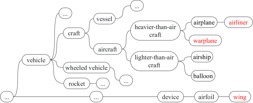
Figure 1. The proposed approach relies on a hierarchical corpus such as ImageNet. The hierarchical corpus is a collection of sets organized as a rooted tree, where each node corresponds to a set and is labelled (e.g. “airplane”). An internal node in the tree is the union of its children. The search algorithm uses both the outputs of the target model and the metadata information provided by the hierarchical corpus to give a most suitable distribution.

4.1. Objective Function

We investigate the data domain of a target model class by class. For each class $i$, we define the objective function as weighted sum of two terms: functional score and semantic score. That is:

$$\alpha\cdot\mathcal{L}_{\mathcal{M}_{i},\mathcal{D}}({\omega_{i}})+(1-\alpha)\cdot\mathcal{S}_{\mathcal{T}}({\omega_{i}})$$

where $\alpha\in(0,1)$ is the weight.

The functional score $\mathcal{L}_{\mathcal{M}_{i},\mathcal{D}}({\omega_{i}})$ combines the goals of responsiveness and transformation invariance by measuring the responsiveness of the model when the dataset $\mathcal{D}_{\omega_{i}}$ is fed into the model with respect to some transformations. The semantic score $S_{\mathcal{T}}({\omega_{i}})$ combines the goals of inclusiveness and common sense and measures how semantically meaningful the selection $\omega_{i}$ is.

Note that input of functional score is a dataset, whereas input of semantic score is the selection parameter.

4.1.1. Functional Score

We define the functional score of a class $i$ in the model with regard to $\mathcal{D}_{\omega_{i}}$ in the following way:

1. Expand $\mathcal{D}_{\omega_{i}}$ by applying uniform random perturbation and a set of transformations including translation, rotation and perspective projection to each data point in $\mathcal{D}_{\omega_{i}}$. We denote this expanded set as $\mathcal{E}(\mathcal{D}_{\omega_{i}})$.

2. The functional score w.r.t $i$-th class is the percentage of the samples in $\mathcal{E}(\mathcal{D}_{\omega_{i}})$ which get classified into it, that is:

   $$\mathcal{L}_{\mathcal{M}_{i},\mathcal{D}}({\omega_{i}})=\frac{|\{{\textbf{x}}\in\mathcal{E}(\mathcal{D}_{\omega_{i}}):\operatorname*{arg\,max}(\mathcal{M}({\textbf{x}}))=i\}|}{|\mathcal{E}(\mathcal{D}_{\omega_{i}})|}$$

To see why this functional score makes sense, we can look at two aspects:

• Firstly, a sensible model should be trained to classify a group of similar objects into a fixed class with high accuracy. Therefore, most samples from the same or very similar distributions should be classified into the same class.

• Secondly, a trained model should have certain transform-invariance to be useful in real life. It should be able to tolerate some noise, translation, rotation, perspective projection, etc. For data distributions which the model is not trained on, such invariance usually does not exist.

4.1.2. Semantic Score

We define the semantic score for a selection $\omega_{i}$ as follows: the semantic score is the average closeness between instances in a selection that is:

$$S_{\mathcal{T}}(\omega_{i})=\frac{\sum_{a\in\omega_{i}}{\sum_{b\in\omega_{i},a\neq b}{CL_{\mathcal{T}}(a,b)}}}{|\omega_{i}|(|\omega_{i}|-1)}$$

We use $CL_{\mathcal{T}}(\cdot,\cdot)$ to denote the closeness between the classes of two samples according to the metadata $\mathcal{T}$ supplied by the hierarchical corpus. For example, the ImageNet consists of 1,000 classes of images organized in the form of a tree. In this tree, for two given nodes, we compute the distance, which is the length of the shortest path between them. The closeness of two instances in the selection is measured by using the inverse of distance of the shortest path between their respective nodes in the tree.

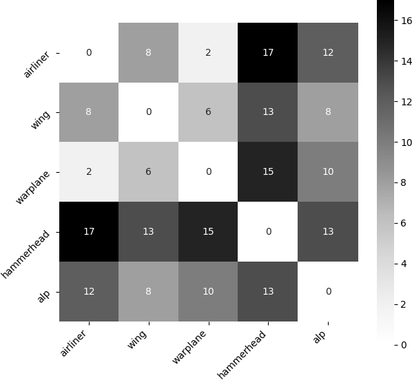
Figure 2. Heat-map of distance matrix among classes in a subset of ImageNet.

To see why this semantic score makes sense, in Figure 2, we show the distance matrix of a small subset of ImageNet. In this small subset, we can observe that for datasets semantically close to airplane, such as airliner, wing and warplane, distances of shortest paths among them are small. In contrast, their distances to the class shark is large.

4.1.3. Remarks

Instead of treating the $n$-class ${\mathcal{D}}_{\omega}$ as a whole, the objectives function is broken down into $n$ parts, each corresponds to a class. Computing the scores separately for each class is helpful when a model classifies very distinct objects with low semantic overlap. For example, a classifier may include cat as one class and airplane as another class.

The overall functional score is defined to be the sum of functional score of each class, that is:

$$\mathcal{L}_{\mathcal{M},\mathcal{D}}({\omega})=\sum_{1}^{n}{\mathcal{L}_{\mathcal{M}_{i},\mathcal{D}}({\omega_{i}})}.$$

Likewise, the semantic score is defined to be the sum of semantic score of each class, that is:

$$S_{\mathcal{T}}(\omega)=\sum_{1}^{n}{S_{\mathcal{T}}({\omega}_{i})}.$$

4.2. Searching for Distributions

We use a heuristic algorithm to search for the solution to our objective function. For each class $i$ of $\mathcal{M}$, we carry out the following steps:

Step 1: Compute the Functional Score.  Suppose there are $m$ leaf nodes in the corpus $\mathcal{C}$, we feed data of each leaf node ${\mathcal{N}}_{j}$ to $\mathcal{M}$ and compute $l_{i,j}=\mathcal{L}_{\mathcal{M}_{i},\mathcal{D}}({\mathcal{N}}_{j})$, for $j=1,\dots,m$.

For example, in CIFAR-10 dataset, the first class has label of ‘airplane’. When using the 1,000 leaf node datasets from ImageNet to compute the functional score, we can rank all datasets according to the score and get following list in Table 1.

Dataset	Score
airliner	0.94
wing	0.92
warplane	0.84
hammerhead shark	0.74
alp	0.60
…	…

Table 1. List of 1,000 classes ranked according to functional score regarding ‘airplane’ class in CIFAR-10.

Step 2: Compute Pairwise Closeness.  We select $l_{i,j}$ that is above a threshold. Let us write these $k$ largest as $l_{i,j_{1}},l_{i,j_{2}},...,l_{i,j_{k}}$. We then compute the pairwise closeness, that is $CL_{\mathcal{T}}(j_{a},j_{b})$ for each $a,b$.

Since datasets in ImageNet are organized in tree hierarchy, we are able to compute the distance of shortest path between any two nodes in the tree. Therefore, we define the closeness of two nodes as the inverse of the distance of shortest path between them.

Step 3: Find a Subset.  From the pairwise closeness table, we can then use an algorithm to find a subset which can maximize the sum of functional score and semantic score.

In our implementation, we run K-medoids (Jin and Han, 2010) algorithm on the pairwise distance matrix. We also compute the distance between centers of clusters. If the distance is lower than a threshold $\eta$ , we merge them into the same cluster. We then choose the cluster with the highest functional score.

Step 4: Filtering.  Now we have a set of nodes (datasets). We would like to only keep the samples which can best represent the target class. For all samples in the chosen datasets, we only keep the data samples which get classified into the target class by the given target model.

5. Evaluation

5.1. Setup

Our evaluation uses five datasets: CIFAR-10 (Krizhevsky et al., 2009), CIFAR-100 (Krizhevsky et al., 2009), Caltech101 (Fei-Fei et al., 2007), Oxford flowers (Nilsback and Zisserman, 2008) and ImageNet (Deng et al., 2009). CIFAR-10 contains 50,000 training images and 10,000 test images. Caltech101 contains 8,677 images in total. Oxford flowers contains 1,020 training images and 6,149 test images. All samples are resized to $32\times 32\times 3$.

In our experimentation, CIFAR-10 and CIFAR-100 are mainly used to train classification models as targets for investigation.

We then exploit the hierarchical information in ImageNet to investigate and find the data distribution of the target classes. The candidate data distribution we found is also used for further investigation: model cloning. These results of investigation are compared with investigation results with same procedure but using Caltech101 and Oxford flowers datasets.

5.2. Evaluation on Functional Requirement

In this section, we test the proposed approach when only functional requirement is applied.

5.2.1. Controlled Environment Test on ImageNet

We first test our method in a controlled environment where we randomly pick 10 classes from the whole 1,000 classes in ImageNet to train a target model. We chose simplified DLA (Yu et al., 2018) as the model architecture. We split the 12,850 images into 10,000 training and 2,850 testing images. This target model achieves 77.0% accuracy.

We then compute the functional score between each class in this target model and each dataset in ImageNet independently using 50 testing images from each dataset. Note the images used in this computation are from testing set of ImageNet and have no overlap with images used in the training process of the target model.

In Table 2, for each target class, we show the datasets with top-2 functional scores. We can observe that the dataset with the highest score is either the exact same class or a very similar class. In addition, the classes with second highest scores are also very close to the target classes.

Original Class	Top 1	Score	Top 2	Score
kit fox	kit fox	0.82	yellow lady’s slipper	0.70
English setter	clumber spaniel	0.86	dalmatian	0.58
Siberian husky	Eskimo dog, husky	0.74	malamute	0.68
Australian terrier	Australian terrier	0.74	silky terrier	0.68
English springer	English springer	0.84	Bernese mountain dog	0.56
grey whale	dugong	0.94	tiger shark	0.90
lesser panda	lesser panda	0.92	ladybug	0.54
Egyptian cat	tabby cat	0.64	leopard	0.60
ibex	ibex	0.88	bighorn	0.60
Persian cat	Persian cat	0.78	mosquito net	0.48

Table 2. Top 2 classes ranked by functional scores for each target class in a classier trained using 10 classes from ImageNet.

5.2.2. CIFAR-10 Classifier

We repeat the same experiment in Section 5.2.1 on a dummy target classifier trained using CIFAR-10 dataset.

We use the same simplified DLA architecture for the target model. For training the target model, we use 45,000 out of 50,000 images in the training dataset of CIFAR-10. This target model achieves 94.9% accuracy.

The remaining 5,000 training images are reserved for the model cloning performance comparison later in Section 5.4.

In Table 3, we can observe the top-1 and top-2 classes are mostly very close to the original class with one exception in the class ‘truck’. This is probably caused by the visual similarity (rectangular shape) between truck and entertainment center.

Original Class	Top 1	Score	Top 2	Score
airplane	airliner	0.94	wing	0.92
automobile	convertible	0.84	sports car	0.84
bird	blue heron	0.88	jay	0.86
cat	tabby cat	0.92	Persian cat	0.92
deer	hartebeest	0.86	impala	0.78
dog	Japanese spaniel	0.94	Dandie Dinmont	0.92
frog	bullfrog	0.74	hen of the woods	0.70
horse	sorrel	0.84	football helmet	0.54
ship	schooner	0.96	drilling platform	0.94
truck	entertainment center	0.96	forklift	0.90

Table 3. Top 2 classes ranked by functional scores for each target class in a classifier trained using CIFAR-10 images.

5.3. Evaluation on Semantic Requirement

Section 5.2.1 shows that the functional score term of objective function works well. In this section, we proceed to test the full objective function with semantic score included. We also use the proposed search algorithm to find the candidate dataset.

Here we set the target classifier as the CIFAR-10 classifier we used in Section 5.2.2. In Table 4, we list the labels of first five classes in CIFAR-10 in the first column. In the second column, we list the names of the datasets which we pick samples from. In the third column, we show the functional scores of the datasets selected by the proposed method, with respect to each class in the target model.

Verify the Results using Label Similarity.   The model predicted a union of classes, and we know the ground truth of each class. However, verifying whether the found distribution is the correct one is not straightforward.

The main challenge is that different datasets may use different terms to refer to a same class, so it is not straightforward to compare two labels and decide whether they are close or distant. For example, how to verify whether the union of classes ‘airliner, wing, warplane, military’ is a good representation of the ground truth ‘airplane’ is not obvious.

Word Embedding.  Word embedding is the representation of words for text analysis, typically in the form of a real-valued vector that encodes the meaning of the word such that the words that are closer in the vector space are expected to be similar in meaning. Word embeddings can be obtained using a set of language modeling and feature learning techniques where words or phrases from the vocabulary are mapped to vectors of real numbers. There are many existing approaches to generate word embedding, for example, word2vec (Mikolov et al., 2013) and GloVe (Pennington et al., 2014).

As different datasets may use different words/phrases to label the same data distribution, word embedding (Mikolov et al., 2013; Pennington et al., 2014) can be useful in checking whether they are referring to the same thing. For example, for the class airplane in CIFAR-10, we have similar classes such as airliner, warplane and wing in ImageNet.

Suppose we can find a candidate distribution of a target class in the unknown model, we can compare the label of this selected distribution and the label of that class in the original training dataset to check whether they are the same or how similar they are. The comparison can be done by measuring the euclidean distance between their word embeddings.

Original Class	Predicted Union of Classes	Func -tional Score	Word -2Vec Score
airplane	airliner, wing, warplane, military plane	0.90	0.581
automobile	convertible, sports car, minivan, beach wagon, station wagon, wagon, estate car	0.78	0.394
bird	little blue heron, Egretta, caerulea, jay, jacamar, magpie, junco, snowbird, ostrich, Struthio camelus	0.75	0.512
cat	tabby cat, Persian cat, Siamese cat, Egyptian cat, tiger cat	0.81	1.000
deer	hartebeest, impala, Aepyceros melampus, gazelle	0.74	0.412

Table 4. Functional score and word2vec cosine similarity of resultant datasets. (w.r.t. first 5 classes in CIFAR-10 target model.)

We use a pre-trained Word2Vec (Mikolov et al., 2013) embedder to compute the cosine similarity between embeddings of labels. For labels which are phrases of multiple tokens, we set the similarity between two phrases as the similarity between their nearest tokens.

We show this similarity score in the last column in Table 4. The results show that the similarities between names of found datasets and their corresponding ground truth labels are high. For a candidate distribution with phrases containing the original class name, we can confirm the selection is good with high confidence. For example, the predicted union of classes for the original class ‘cat’ is good as it contains all specific breeds of cats.

In Figure 3, we visualize word embeddings of the labels found by the proposed method and ground truths by mapping them to two-dimensional space using t-distributed stochastic neighbor embedding (t-SNE). We can see the labels found by the proposed method are indeed close to their corresponding ground truths in the embedding space.

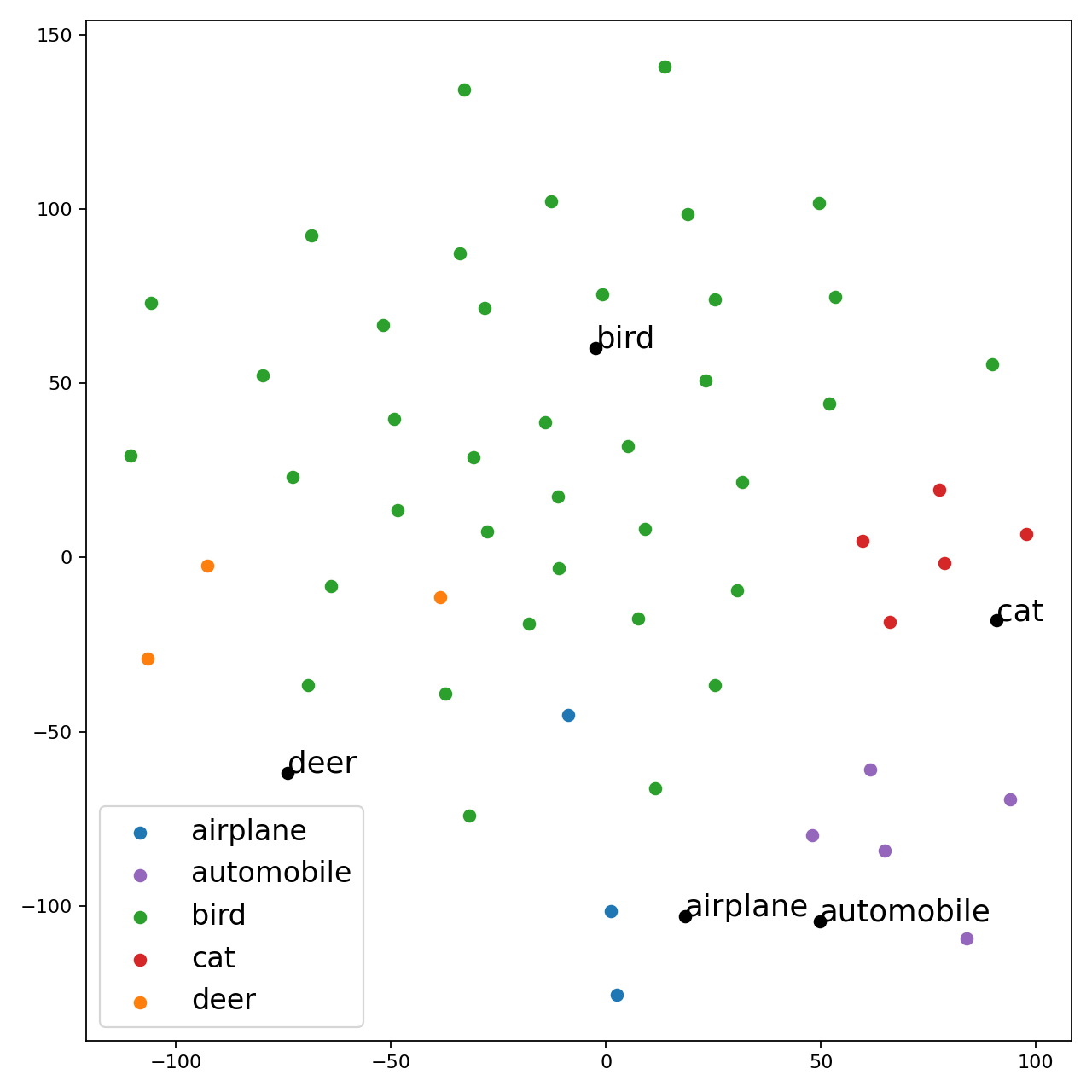
Figure 3. t-SNE visualization of embeddings of ground truths labels and labels obtained through the proposed method.

5.4. Further Investigation: Model Cloning

To further evaluate the adequacy of the datasets found by the proposed method, we conduct model cloning by using the found datasets as auxiliary datasets. We compare the performance of cloning using: (1) Same Distribution: clone using the same CIFAR distribution (split data); (2) Similar Distribution: clone using Caltech101 dataset; (3) Distant Distribution: clone using Oxford flowers dataset. (4) Clone using randomly sampled subset from ImageNet.

5.4.1. Target Model: CIFAR-10 Classifier

We first use the target model (with simplified DLA architecture) in Section 5.2.2. As this model was using 45,000 training images of CIFAR-10, we use remaining 5,000 training images to conduct model cloning. The accuracy of the target model is shown in Table 5 column 2.

We use GoogLeNet (Szegedy et al., 2015) as the cloned model’s architecture and train each clone for 200 epochs. Here we follow Papernot et al.’s method of cloning (Papernot et al., 2017). The accuracy for each class and overall accuracy is shown in Table 5 column 3. We then repeat the same cloning procedure for two different dataset: Caltech101 (column 4) and Oxford flowers (column 5). We also only use 5,000 images from each dataset and use the same GoogLeNet architecture. For comparison, we also randomly sample 5,000 images from ImageNet without using the search algorithm to conduct cloning (column 6).

We then conduct the same model cloning process for datasets found by the proposed method. For fair comparison, the dataset found by proposed method also contains 5,000 images in total. Column 7 shows the cloning performance using the datasets we found based on the first term (functional score) of the objective function. Column 8 shows the performance when both functional score and semantic score are considered.

In Table 5, we can observe that cloning using the same distribution gives the highest accuracy. Caltech101 contains many similar classes as the target model, for example, passenger vehicles and animals, thus has a relatively high cloning accuracy. In contrast, Oxford flowers only contains images of flowers, therefore results in the lowest cloning accuracy.

With only one term of the objective function enabled, the performance of the proposed method has already surpassed randomly sampling data from ImageNet. We can observe that the performance is better with both terms enabled since the obtained datasets are more semantically meaningful.

Class	Target Model	CIFAR 10	Caltech 101	Oxford Flowers	Image -Net	Extract using 1 term	Extract using 2 terms
airplane	95.3%	84.5%	73.7%	72.7%	35.8%	78.9%	76.6%
automobile	97.8%	90.7%	0.1%	0.0%	44.6%	94.1%	92.9%
bird	92.8%	68.1%	17.2%	24.7%	15.2%	39.1%	43.3%
cat	88.6%	74.7%	77.1%	68.1%	41.3%	71.2%	74.4%
deer	96.6%	80.8%	72.4%	49.7%	46.5%	61.2%	70.3%
dog	91.9%	69.2%	3.4%	4.0%	54.0%	61.4%	77.7%
frog	97.4%	86.2%	72.7%	65.4%	20.1%	64.4%	78.5%
horse	96.5%	78.5%	0.3%	0.0%	31.1%	53.9%	57.8%
ship	96.0%	90.7%	83.8%	59.6%	43.2%	67.4%	68.9%
truck	96.4%	89.8%	54.3%	0.0%	23.2%	38.7%	79.8%
Average	94.9%	81.3%	45.5%	34.4%	35.5%	63.0%	72.0%

Table 5. Comparison of accuracy of models cloned by using various given datasets and models cloned by using datasets extracted with the proposed method.

5.4.2. Target Model: CIFAR-100 Classifier

We repeat the same experiment of model cloning on a target model with same architecture but trained using CIFAR-100. The model was also trained using 45,000 images and 5,000 images were reserved for testing the cloning performance from same distribution. This target model achieves 76.4% accuracy.

As there are 100 classes in CIFAR-100, we are unable to show a full table of accuracy here. We show the KDE (Kernel density estimation) plot instead. The horizontal axis shows the accuracy and the vertical axis shows the density.

In Figure 4, we can observe that the result is similar to what we have seen on CIFAR-10. The dataset obtained through the proposed method yields much better cloning accuracy than a hand-picked distribution that is seemingly close to the training distribution.

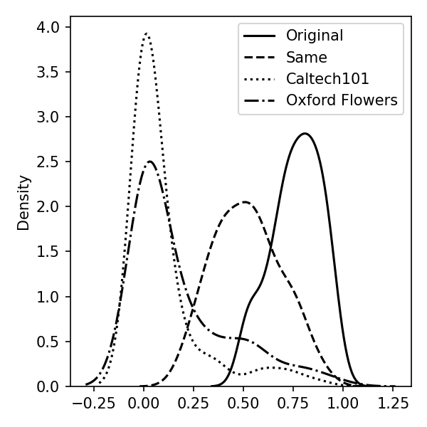
(a) Original model vs.
model cloned using CIFAR-100,
Caltech101 and Oxford Flowers
datasets.

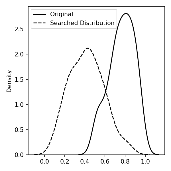
(b) Original model vs.
model cloned using datasets
obtained through the proposed
approach.

Figure 4. KDE plot of accuracy of each class (100 classes).

5.5. Field Experiment: Hugging Face Model Hub

The Hugging Face platform stores over 60,000 machine learning models. These model are mostly open source and can be directly downloaded.

While most models have detailed documentations, some only provide the code to load the checkpoints without any description of the purpose/usage of the model. In this section, we randomly pick two undocumented models and use the proposed method to investigate them. There is no documentation of the models in these two repositories at the time of submission of this manuscript.

First Example:
https://huggingface.co/Matthijs/mobilenet_v2_0.75_160.
This model has 1,000 classes. There seems to be a resemblance between the training data distribution of this model and ImageNet. For 991 out of 1,000 classes, the search algorithm converges to a leaf node in ImageNet with average functional score of 0.77. In addition, more than 75% of the classes have their functional scores higher than 0.9. Further analysis shows that the indices of classes in this unknown model also match well with the class indices of leaf nodes found by the search algorithm. When we treat the unknown model as an ImageNet classifier, it can achieve 69.5% accuracy on the testing dataset and 99.5% accuracy on the training dataset. Therefore, based on these evidences, we highly suspect that this model is trained using ImageNet dataset.

Second Example:
https://huggingface.co/nateraw/timm-resnet50-beans-copy.
This model has three classes. The search algorithm matches all three classes to node n00017222 (plant, flora, plant life) in ImageNet with functional score of 0.81, 0.74, 0.72 respectively. We visually inspected node n00017222 and found out that n00017222 consists of two classes: yellow lady’s slipper and daisy. Most images contain both flowers and leaves. As the node has quite limited number of images, in our attempt to find out the exact classes of the unknown classifier, we apply two other datasets in our investigation: Oxford flowers (Nilsback and Zisserman, 2008) and Flavia leaf dataset (Wu et al., 2007).

As both Oxford flowers and Flavia leaf dataset are not hierarchical datasets, here our analysis relies on the functional score only. When using Oxford flowers, the functional scores are generally low with an average of only 0.36. On the other hand, on Flavia leaf dataset, the average functional score is 0.83, which is even higher than the average score of node n00017222.

Flavia leaf dataset contains 1,907 images from 33 classes of leaves. Among all the classes, the class ‘Cercis chinensis’ has the highest average functional score of 0.90.

In Figure 5, we show four samples with the highest functional scores for the first class of the unknown model (left is the highest). Cercis chinensis is a plant from the bean family. It is possible that the unknown model is a classifier for some leaves visually similar to bean leaves.

Figure 5. Four samples with the highest functional scores in Flavia leaf dataset.

6. Future Works

6.1. Requirement on Hierarchical Datasets

The proposed method is able to find distributions that are close to the training distribution of a black-box model if such close distributions exist in the given hierarchical corpus. When running the algorithm for a model with no similar distribution in the corpus, it returns a ‘not found’ result.

Constructing a more comprehensive hierarchical corpus relies on community effort. Over the past few years, we have seen large datasets such as Google’s JFT-3B (Zhai et al., 2021) which was annotated with a class-hierarchy of around 30k labels. There are also large hierarchical dataset for specific domain such as Stanford Medical ImageNet (med, [n. d.]). However, these datasets are not publicly available yet.

While ImageNet is far from being comprehensive, it is a good starting point. As a hierarchical corpus, it is very expandable. For each specific investigation task, we can add our data to a node in the ImageNet hierarchy. Based on our experience in Section 5.5, the process is straightforward and the outcome is promising.

In addition, with recent breakthrough in generative models, it becomes possible to generate images to expand a given corpus. For example, one limitation of ImageNet is the lack of X-ray images. We can use stable diffusion to generate a large set of X-ray images (shown in Figure 6), organized them in the form of a tree and add them to ImageNet as a subtree. Although they may contain errors sometimes, most images are good enough for analysis under the proposed method. Similarly, we can also generate new data for ‘leaf’, even for samples like blue maple and white maple which do not exist in real life (shown in Figure 6).

When a candidate distribution is extracted from a hierarchical corpus, the images are guaranteed to be meaningful natural images. However, when using generative models, additional constraints may be required to make sure the selected datasets contain semantically meaningful objects. Certain distributions of noises, artifacts or adversarial images may fulfill functional requirements but will not be useful for forensic investigation.

In Figure 6, the process of expanding the hierarchical corpus was done manually. An automatic workflow can also be easily implemented. Testing samples can be generated ‘on the fly’ with prompts progressively narrow down from a general concept to a specific object. The research on such algorithm will be an interesting future work.

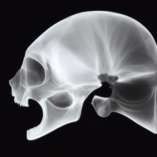
(a) Cat X-ray.

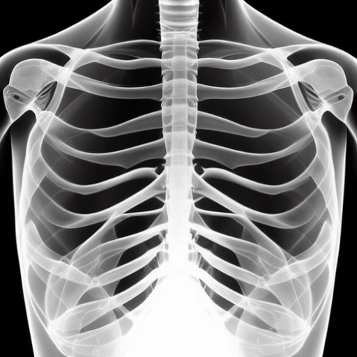
(b) Chest X-ray.

(c) Blue maple.

(d) White maple.

Figure 6. Examples of generated samples in new subtrees.

Another important future work will be applying the proposed method to unknown models trained using other data types such as text and graph. Our objective function and search method are compatible with different data types since we use a model’s hard label output regardless of the internal architecture. Theoretically, changing to a hierarchical corpus of other data type will work without additional modification.

6.2. Use as an Attack and Potential Countermeasures

The proposed method is a powerful tool for forensic investigation. However, it may be used for attacks as well. While there are some relevant works on potential defenses, they are mostly for data protection during federated learning (Huang et al., 2020) or running on untrusted hardware (Alam et al., [n. d.]).

Since the attack is new, we designed a custom countermeasure which may potentially work. We propose hiding the real input distribution of a model by adaptively planting some back-doors which generate strong signals that confuse the investigator/attacker.

We trained a MNIST (LeCun et al., 2010) classifier to verify our hypothesis. The model is trained in such way: We use the usual 60,000 training images; We pair the 10 classes in MNIST with the 10 classes in CIFAR-10; For each class in MNIST, we add 500 additional training images from their respective CIFAR-10 class to inject the back-doors. We use simplified DLA as the architecture. The model was trained for 200 epochs and reached 99.2% accuracy.

When running the proposed search algorithm on this classifier using ImageNet as the corpus, it returns datasets which are obviously more related to the CIFAR-10 classes. For example, the digit $0$ was paired with the airplane class during training. The search result for this class was ‘wing, airliner, warplane and airship’ with a high functional score at 0.745.

7. Conclusion

We highlight that knowing the data domain of a model is a necessary first step before conducting further investigation. We present a method that allows us to extract a meaningful distribution that is similar to the model’s input data distribution from a hierarchical dataset. The experimentation results show that the proposed method is highly useful and very accurate even with only black-box and hard-label only access to the target model being investigated. In addition, when using the dataset obtained through the proposed method to conduct model cloning, the performance is much better than manually choosing a similar distribution to clone. We also discussed potential countermeasures which could be employed to hinder the proposed investigation method.

References

- (1)
- med ([n. d.]) [n. d.]. Medical ImageNet. https://aimi.stanford.edu/research/medical-imagenet. Accessed: 2022-01-28.
- Alam et al. ([n. d.]) Mohammad Mahmudul Alam, Edward Raff, Tim Oates, and James Holt. [n. d.]. Deploying Convolutional Networks on Untrusted Platforms Using 2D Holographic Reduced Representations. In ICML.
- Chen et al. (2020) Dingfan Chen, Ning Yu, Yang Zhang, and Mario Fritz. 2020. GAN-Leaks: A Taxonomy of Membership Inference Attacks against Generative Models. In CCS. ACM, 343–362.
- Deng et al. (2009) Jia Deng, Wei Dong, Richard Socher, Li-Jia Li, Kai Li, and Fei-Fei Li. 2009. ImageNet: A large-scale hierarchical image database. In CVPR. 248–255.
- Dosovitskiy and Brox (2016a) Alexey Dosovitskiy and Thomas Brox. 2016a. Generating Images with Perceptual Similarity Metrics based on Deep Networks. In NIPS. 658–666.
- Dosovitskiy and Brox (2016b) Alexey Dosovitskiy and Thomas Brox. 2016b. Inverting Visual Representations with Convolutional Networks. In CVPR. 4829–4837.
- Fei-Fei et al. (2007) Li Fei-Fei, Robert Fergus, and Pietro Perona. 2007. Learning generative visual models from few training examples: An incremental Bayesian approach tested on 101 object categories. Comput. Vis. Image Underst. 106, 1 (2007), 59–70.
- Fredrikson et al. (2015) Matt Fredrikson, Somesh Jha, and Thomas Ristenpart. 2015. Model Inversion Attacks that Exploit Confidence Information and Basic Countermeasures. In ACM CCS. 1322–1333.
- Huang et al. (2020) Yangsibo Huang, Zhao Song, Kai Li, and Sanjeev Arora. 2020. InstaHide: Instance-hiding Schemes for Private Distributed Learning. In ICML, Vol. 119. 4507–4518.
- Jia et al. (2019) Jinyuan Jia, Ahmed Salem, Michael Backes, Yang Zhang, and Neil Zhenqiang Gong. 2019. MemGuard: Defending against Black-Box Membership Inference Attacks via Adversarial Examples. In CCS. ACM, 259–274.
- Jin and Han (2010) Xin Jin and Jiawei Han. 2010. K-Medoids Clustering. In Encyclopedia of Machine Learning. 564–565.
- Krizhevsky et al. (2009) Alex Krizhevsky et al. 2009. Learning multiple layers of features from tiny images. (2009).
- LeCun et al. (2010) Yann LeCun, Corinna Cortes, and CJ Burges. 2010. MNIST handwritten digit database. ATT Labs, http://yann.lecun.com/exdb/mnist (2010).
- Lee and Kil (1994) Sukhan Lee and Rhee Man Kil. 1994. Inverse mapping of continuous functions using local and global information. IEEE Trans. Neural Networks 5, 3 (1994), 409–423.
- Li and Zhang (2020) Zheng Li and Yang Zhang. 2020. Label-Leaks: Membership Inference Attack with Label. CoRR abs/2007.15528 (2020).
- Lowd and Meek (2005) Daniel Lowd and Christopher Meek. 2005. Adversarial learning. In ACM SIGKDD. 641–647.
- Lu et al. (1999) Bao-Liang Lu, Hajime Kita, and Yoshikazu Nishikawa. 1999. Inverting feedforward neural networks using linear and nonlinear programming. IEEE Trans. Neural Networks 10, 6 (1999), 1271–1290.
- Mahendran and Vedaldi (2015) Aravindh Mahendran and Andrea Vedaldi. 2015. Understanding Deep Image Representations by Inverting Them. In CVPR. 5188–5196.
- Mikolov et al. (2013) Tomas Mikolov, Kai Chen, Greg Corrado, and Jeffrey Dean. 2013. Efficient Estimation of Word Representations in Vector Space. arXiv:1301.3781 [cs.CL]
- Milli et al. (2019) Smitha Milli, Ludwig Schmidt, Anca D. Dragan, and Moritz Hardt. 2019. Model Reconstruction from Model Explanations. In FAccT. 1–9.
- Nash et al. (2019) Charlie Nash, Nate Kushman, and Christopher K. I. Williams. 2019. Inverting Supervised Representations with Autoregressive Neural Density Models. In AISTATS, Vol. 89. 1620–1629.
- Nilsback and Zisserman (2008) M-E. Nilsback and A. Zisserman. 2008. Automated Flower Classification over a Large Number of Classes. In Proceedings of the Indian Conference on Computer Vision, Graphics and Image Processing.
- Oh et al. (2019) Seong Joon Oh, Bernt Schiele, and Mario Fritz. 2019. Towards Reverse-Engineering Black-Box Neural Networks. In Explainable AI: Interpreting, Explaining and Visualizing Deep Learning. Lecture Notes in Computer Science, Vol. 11700. 121–144.
- Orekondy et al. (2019) Tribhuvanesh Orekondy, Bernt Schiele, and Mario Fritz. 2019. Knockoff Nets: Stealing Functionality of Black-Box Models. In CVPR. 4954–4963.
- Papernot et al. (2017) Nicolas Papernot, Patrick D. McDaniel, Ian J. Goodfellow, Somesh Jha, Z. Berkay Celik, and Ananthram Swami. 2017. Practical Black-Box Attacks against Machine Learning. In AsiaCCS. 506–519.
- Pennington et al. (2014) Jeffrey Pennington, Richard Socher, and Christopher Manning. 2014. GloVe: Global Vectors for Word Representation. In EMNLP. 1532–1543.
- Rahman et al. (2018) Md. Atiqur Rahman, Tanzila Rahman, Robert Laganière, and Noman Mohammed. 2018. Membership Inference Attack against Differentially Private Deep Learning Model. Trans. Data Priv. 11, 1 (2018), 61–79.
- Salem et al. (2019) Ahmed Salem, Yang Zhang, Mathias Humbert, Pascal Berrang, Mario Fritz, and Michael Backes. 2019. ML-Leaks: Model and Data Independent Membership Inference Attacks and Defenses on Machine Learning Models. In NDSS. The Internet Society.
- Schunter (2016) Matthias Schunter. 2016. Intel Software Guard Extensions: Introduction and Open Research Challenges. In Proceedings of the 2016 ACM Workshop on Software PROtection (SPRO ’16). Association for Computing Machinery.
- Shokri et al. (2017) Reza Shokri, Marco Stronati, Congzheng Song, and Vitaly Shmatikov. 2017. Membership Inference Attacks Against Machine Learning Models. In IEEE S&P. 3–18.
- Szegedy et al. (2015) Christian Szegedy, Wei Liu, Yangqing Jia, Pierre Sermanet, Scott E. Reed, Dragomir Anguelov, Dumitru Erhan, Vincent Vanhoucke, and Andrew Rabinovich. 2015. Going deeper with convolutions. In CVPR. 1–9.
- Tramèr et al. (2016) Florian Tramèr, Fan Zhang, Ari Juels, Michael K. Reiter, and Thomas Ristenpart. 2016. Stealing Machine Learning Models via Prediction APIs. In USENIX.
- Wang and Gong (2018) Binghui Wang and Neil Zhenqiang Gong. 2018. Stealing Hyperparameters in Machine Learning. In IEEE S&P. 36–52.
- Wu et al. (2007) Stephen Gang Wu, Forrest Sheng Bao, Eric You Xu, Yuxuan Wang, Yi-Fan Chang, and Qiao-Liang Xiang. 2007. A Leaf Recognition Algorithm for Plant Classification Using Probabilistic Neural Network. arXiv preprint 0707.4289 (2007). arXiv:0707.4289
- Yang et al. (2019) Ziqi Yang, Jiyi Zhang, Ee-Chien Chang, and Zhenkai Liang. 2019. Neural Network Inversion in Adversarial Setting via Background Knowledge Alignment. In ACM CCS. 225–240.
- Yu et al. (2018) Fisher Yu, Dequan Wang, Evan Shelhamer, and Trevor Darrell. 2018. Deep Layer Aggregation. In CVPR. 2403–2412.
- Zhai et al. (2021) Xiaohua Zhai, Alexander Kolesnikov, Neil Houlsby, and Lucas Beyer. 2021. Scaling Vision Transformers. CoRR abs/2106.04560 (2021).