A Statistical Model of Bipartite Networks: Application to Cosponsorship in the United States Senate††thanks: The methods described in this paper can be implemented via the open-source statistical software, NetMix, available at https://CRAN.R-project.org/package=NetMix. The authors are grateful for comments from Alison Craig, Skyler Cranmer, Sarah Shugars and the participants of the Harvard IQSS Applied Statistics seminar.
Abstract
Many networks in political and social research are bipartite, with edges connecting exclusively across two distinct types of nodes. A common example includes cosponsorship networks, in which legislators are connected indirectly through the bills they support. Yet most existing network models are designed for unipartite networks, where edges can arise between any pair of nodes. We show that using a unipartite network model to analyze bipartite networks, as often done in practice, can result in aggregation bias. To address this methodological problem, we develop a statistical model of bipartite networks by extending the popular mixed-membership stochastic blockmodel. Our model allows researchers to identify the groups of nodes, within each node type, that share common patterns of edge formation. The model also incorporates both node and dyad-level covariates as the predictors of the edge formation patterns. We develop an efficient computational algorithm for fitting the model, and apply it to cosponsorship data from the United States Senate. We show that senators tapped into communities defined by party lines and seniority when forming cosponsorships on bills, while the pattern of cosponsorships depends on the timing and substance of legislations. We also find evidence for norms of reciprocity, and uncover the substantial role played by policy expertise in the formation of cosponsorships between senators and legislation. An open-source software package is available for implementing the proposed methodology.
Keywords: affiliation network, mixed-membership model, social network, stochastic block model, variational inference
1 Introduction
Bipartite networks — or networks in which ties connect actors of two distinct types, and no such connections occur between actors of the same type — are commonly encountered in political and social research. Examples include ethnic group memberships of individuals [34, e.g.], policy adoption among U.S. states [10, e.g. ], and product-level trade between countries [29, e.g.]. Such networks, sometimes known as affiliation networks, are also common in other domains: customer-product relationships [25, e.g], actor-movie ties [41, e.g.], and even document-word occurrences of the kind typically used in text-as-data analyses [32, e.g.] can be represented as bipartite networks.
Despite their ubiquity, the most popular approach to analyzing affiliation networks is to recode them as unipartite network data, containing information about the relationships among only one type of node. For example, consider a bipartite network of legislative cosponsorships, in which legislators and bills represent two separate types of nodes with ties occurring only between these two groups rather than within them. When analyzing these type of data, researchers typically project (or aggregate) this bipartite network onto a unipartite network of legislators by defining an edge between two legislator nodes as capturing the existence (or the number) of cosponsored bills between them [47, 38, see, e.g.,].
In fact, such projections are a common practice whenever researchers analyze naturally bipartite networks. After examining recent publications in top political science journals, we found that 30 (or nearly 40%) of the 77 articles which use some type of network data study originally bipartite networks. And among these, all but two papers project them onto unipartite networks (see Table A.1 in Appendix A.1).
The popularity of this projection strategy is not surprising, given that the most commonly used statistical models of static network formation in the social sciences — typically some variant of the latent-space model [23] or the exponential random graph model [16, 49, or ERGM;] — were originally designed for unipartite networks. This is also true for more recently proposed modeling approaches to network cross-sections, including the generalized ERGM [9], the additive and multiplicative effects model [37], and the stochastic blockmodel (SBM) [27, e.g.,].
Unfortunately, as we show below, the projection of a bipartite network onto a unipartite network leads to loss of information, possibly resulting in misleading estimates of the determinants of network ties. To avoid the needs for bipartite projections and minimize the risk of inducing such biases, we extend the popular mixed membership stochastic block model (MMSBM; [1]) to bipartite networks. The proposed model allows researchers to identify the groups of nodes, within each node type, that share common patterns of edge formation (so called stochastic equivalence classes). In the aforementioned cosponsorship example, the model characterizes how different groups of legislators cosponsor different types of bills — thus classifying legislators and bills into their own, substantively meaningful groups.
Our model is based on a mixed-membership (or admixture) structure, where a node of one type can belong to different latent groups depending on which nodes of the other type they are interacting with. This flexibility allows us to capture nuanced social interactions in which actors adopt different roles when interacting with others. This contrasts with most of the existing bipartite community detection models that assume every node (or every edge) belongs to a single group [18, 33, 52, 28, e.g.]. In cosponsoring networks, for example, a legislator may cooperate with a different group of their colleagues when considering the cosponsorship of bills in different policy areas. Thus, our model can capture the complexity of social networks by modeling a wide range of edge formation patterns.
In addition, for any given node of one type, our model allows the use of covariates to explain the patterns of edge formation with different nodes of the other type [50, 44]. In the cosponsorship network, for instance, specific legislation may invite support based on similar policy content in some instances, and through the sponsor’s influence and characteristics in others.
To accommodate such situations, our model incorporates two types of covariates, allowing researchers to evaluate social science theories. First, one can use node-level covariates to characterize group memberships. In the cosponsorship example, we can use the characteristics of legislators (e.g., ideologies, partisanship) and those of bills (e.g., contents, sponsor’s characteristics) to understand their respective latent group memberships. Second, the model also allows for the use of dyadic covariates to directly predict edge formation. This feature is helpful when a variable is defined for a pair of nodes of different types (e.g., whether a legislator is a member of the committee which drafted a bill).
In contrast, many existing modeling approaches often force researchers to adopt a two-step analyitics strategy, conducting standard regression analyses of network model outputs [36, 21, 51, 7, 47, 3, e.g.] By offering a single-step, comprehensive approach to network data analysis, our model can be used by researchers who wish to evaluate social science theories or those who wish to make predictions on new sets of actors.
One disadvantage of MMSBM-type network models is that a fully Bayesian inference strategy relying on Markov chain Monte Carlo simulation is computationally too expensive for networks of medium or large size. To overcome this problem, we follow the computational strategy used in the existing methodological literature and develop a computationally efficient variational Bayes approximation to our model’s collapsed posterior using stochastic optimization [48, 1, 24, 17, 40]. We implement this fitting algorithm in the open-source software package NetMix [39] so that other researchers can use the proposed model in their own research.
Using our proposed approach, we study the patterns of legislative cosponsorship during the 107th Congress of the U.S. Senate, modeling the two-mode network connecting Senators to legislation (or “bills”). Our model identifies a group of senators who collaborate across party lines to cosponsor a certain type of bills. The unipartite version of the model fails to detect this pattern. Specifically, we identify the important role played by up-and-rising junior senators from both parties in generating cross-aisle collaboration. In addition, the model shows that after senator Jeffords’ split from the Republican party and the events on 9/11, the senate becomes more collaborative on security-related legislation. We also identify the critical role of committee memberships, and find evidence of bill-specific norms of reciprocity in cosponsorship — a phenomenon that would be lost if we focused on aggregate network measures.
In what follows, we discuss our motivating application — the politics of cosponsorship in the U.S. — and explain the risk of aggregation bias when projecting bipartite networks to unipartite networks (Section 2). We then discuss the details of our modeling approach in Section 3, and present the results of our empirical analysis of the cosponsorship networks during the 107th Congress in Section 4. Finally, in Section 5, we conclude with a discussion about the applicability of our model to other domains.
2 The Cosponsorship Network Among Senators
In this section, we introduce the cosponsorship network data among legislators in the U.S. Senate, which serves as our motivating example. We point out the bipartite nature of the data and explain why projecting this bipartite network onto a unipartite one results in loss of information and possibly aggregation bias.
2.1 Background
Cosponsorship relationships among U.S. senators offer a useful window into their legislative interests and goals, as they indicate willingness to publicly and directly endorse a particular piece of legislation [47, 2, 30, see e.g.,]. For senators, cosponsorship is important because the rules of Senate constrain sponsorship to a single legislator. Thus, cosponsorships often indicate broader support for the content of the legislation or sponsoring legislator and increases media attention [31]. Previous work has noted the importance of collaboration among senators in legislative productivity and influence [15]. Scholars have been interested in questions on when senators are most likely to cosponsor legislation, whether this is prompted by both legislation- and legislator-specific factors (such as bill content and/or senatorial seniority), and how senatorial experience and expertise might influence cosponsorship behaviors [6, 31, 20, 12, see, among others,].
2.2 Cosponsorships during the 107th Senate
In exploring these questions, we focus on the 107th Senate, which was in session between 2001 and 2003, as the presidency transitioned from the Clinton to Bush administration. The 107th Senate was eventful by many standards. Aside from battles over health care policy, education bills and investigations and rewriting of election laws after the tumultuous 2000 presidential election, party control of the Senate changed hands as well. During the two years, control of the Senate flipped from a narrow Republican control where the G.O.P. could mostly enact policy through convincing a handful of Democrat colleagues in a 50-50 Senate split (where Vice President Dick Cheney gave the Republicans their narrow edge) to a likewise razor-thin advantage towards the Democrats in June 2001 once Jim Jeffords defected from the Republican party as an Independent and began to caucus in earnest with Democrats. Finally, 9/11 shook the domestic agenda altogether, and ramped up foreign policy and security as priority in both parties, seeing the beginnings of the subsequent “War on Terror” and making bipartisan shows of unity all the more important in a time when national security was at the forefront of the national debate.
Before 2021, the Senate had only been perfectly split three other times, with the 107th being the most recent instance of this rare event in the Senate’s history. Despite this, the 107th Senate was not unusual in terms of its productivity, passing about 17% of the 3,242 pieces of legislation introduced between 2000 and 2002 — close to the average of 22% approval rate during the modern Senate. There were a total of 20,660 instances of cosponsorships where a senator attached his/her name to a piece of legislation. We represent these senator-bill relations as a bipartite network, in which senators and legislations represent two separate groups of nodes and edges occur between two nodes only across the groups and not within each group.
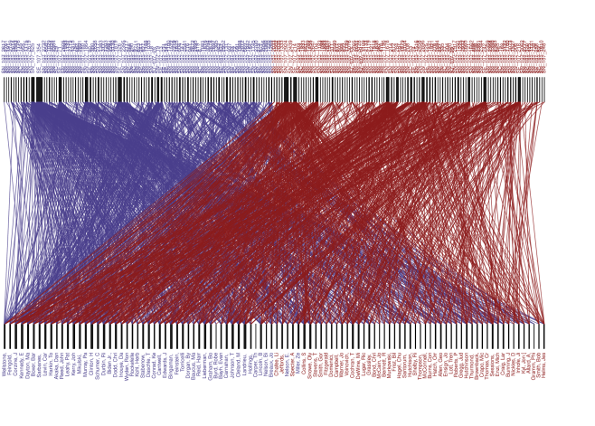
Figure 1 presents this bipartite network based on 100 senators (bottom nodes) and a randomly selected sample of 200 bills (top nodes). Edges as well as the name of each bill are colored based on the partisanship of the bill’s original sponsor. We observe a substantial degree of heterogeneity in cosponsorship behavior: some bills attract many cosponsors (represented by thick black vertical lines) while others have relatively few (thin lines). While many bills are supported by senators from both parties, certain legislation is only cosponsored by senators whose partisanship is the same as that of their sponsors (represented by edges between two nodes of the same color).
Much as senators might differentially decide to cosponsor based on their personal characteristics, so too might legislation attract cosponsorship based on content and the context in which it is introduced. We observe rich information levied off of senators as well as the legislation itself. We collect senator-specific covariates (such as party, ideology, seniority, and sex) for the Congress, and information on the class (e.g. resolutions or bills), major category of the legislation (measured as a categorical variable with levels for substantive content on issues of the economy, international topics, social and public programs, security, government operations, and all uncategorized legislation as “other”), and the phase in Congress it was introduced (pre-Jeffords’ split, post-Jeffords’ split, post 9/11) from the Congressional cosponsorship data in [14].
Two substantial predictors of cosponsorship decision occur at the senator-bill dyad level. First, senators often trade favors amongst one another, such that cosponsorship may result from quid pro quo behavior — “you cosponsored me before, I’ll cosponsor you now” [4]. We can capture this reciprocal behavior through investigating, in a given senator-bill dyad in the 107th Congress, how often the sponsor of the bill in question previously cosponsored the other senator in the dyad in the 106th Congress out of all the opportunities they could have cosponsored this particular senator. As this reciprocity variable relies on a denominator of having sponsored bills in Congress 106 and is skewed to the right, we incorporate two variables capturing reciprocity: a binary variable encoding whether no reciprocity exists, and a variable capturing the log of the reciprocity proportion.
Second, scholars have increasingly stressed the importance of the power of Senate committees in forming support around legislation, not least because senatorial experience and expertise increases with oversight of the bill in question within a committee the Senator herself sits on [43, 8]. We gather Senator committee and bill committee information from [46] and ProPublica Congress Bill API,111See https://projects.propublica.org/api-docs/congress-api/bills/ respectively, and consider a senator-bill dyad sharing a committee if a senator has sat on a committee that the bill passed through.
2.3 Projection onto a unipartite network can be misleading
How do researchers analyze bipartite networks like the one shown in Figure 1? As mentioned earlier, the most common approach is the projection of a bipartite network onto a unipartite network. In the current application, one may turn the senator-bill bipartite network into a unipartite network of senators where an edge between two senators represents whether or not they cosponsor a bill together (or the number of such bills, in the case of a weighted unipartite network), such as done in [47]. In adopting this strategy, however, researchers risk losing relevant information on the details of policy content and on attributes that are defined at the bill level as well as the senator-bill dyadic level. Indeed, this loss of bill-related information is particularly problematic when using cosponsorship decisions as “indicators of members’ purest form of issue positioning” [35].
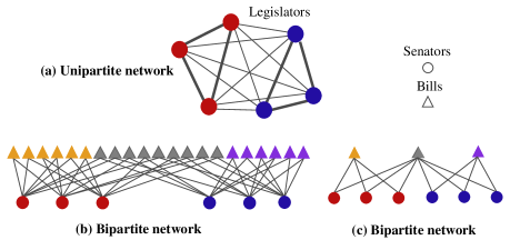
Aggregating over potentially relevant heterogeneity in bill- and senator-bill level data can directly lead to incorrect substantive takeaways. To see how this may be the case, consider a stylized scenario presented in Figure 2. The simple weighted unipartite representation of a cosponsorship network is shown in panel (a) of the figure. In this graph, senators are nodes (circles, color differentiated by party affiliation) with weighted edges drawn between senators that cosponsor at least one piece of legislation, with weights given by the number of times such cosponsorships happen. A cursory view of this graph might suggest that while there is some cross-party cosponsorship, there is much more frequent within-party collaboration.
Yet this same unipartite representation can be derived from completely different bipartite network structures. At the bottom of Figure 2, bipartite networks (b) and (c) incorporate the missing bill information, and represent two very different legislative environments that nevertheless project onto the same unipartite network form presented in panel (a). In panel (b), legislators are highly productive in terms of legislative output (given by the large number of triangular nodes in the graph), and frequent cross-party work is common (as indicated by the relatively large number of gray triangular nodes in the graph). Indeed, the bipartisan vs. within-party cosponsored legislation ratio is 3 to 4.
The graph in panel (c) tells a different story altogether. Senators in panel (c) are far less productive in individual bills, more unified in terms of within party cosponsorships, and collaborate only once across the aisle through a single, widely cosponsored bill.222In formal graph-theoretic terms, the vertex connectivity of network (c) is much smaller than that of network (b), with a cutset of only a single gray bill cosponsored by all legislators: it would only take removing the single shared gray (triangle) bill to separate the network into two distinct components. Likewise, the bipartisan versus within-party cosponsored legislation ratio is much lower — namely, 1 to 2. This substantive differentiation of bipartisan versus polarized behavior is completely obscured in Figure 2 (a), even after weighting edges according the number bills through which cosponsorship happens.
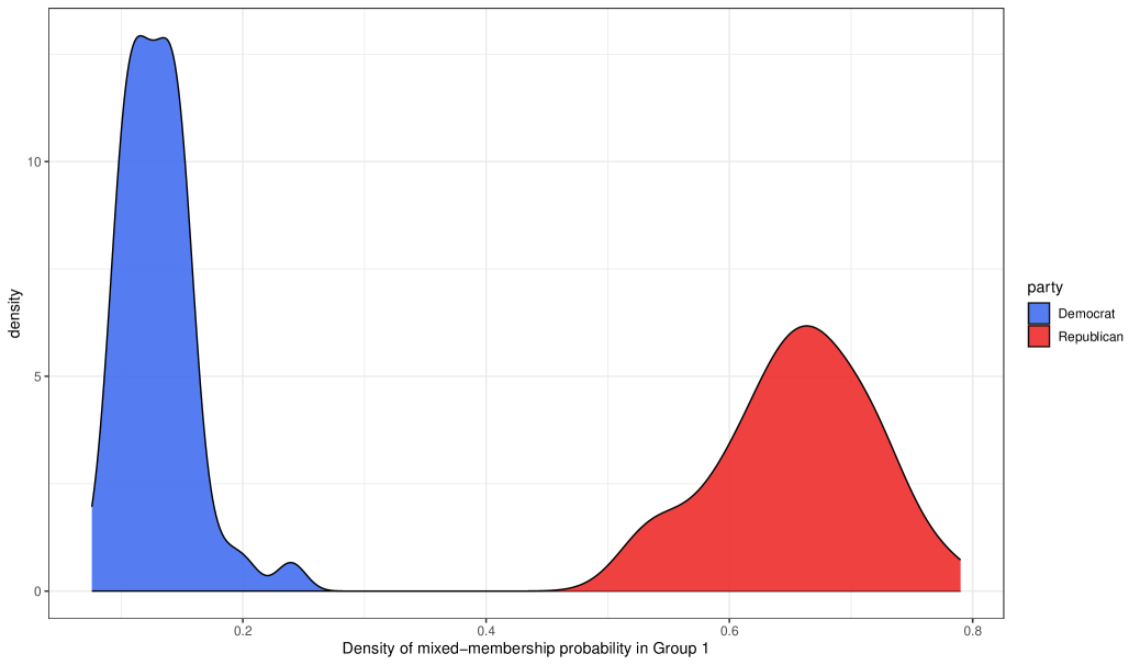
This kind of aggregation bias is palpable in the 107th Senate. If we were to study cosponsorship decisions after projecting them onto a senator-only network, we would be left with little clue as to why this session remained reasonably productive despite the stark partisan divisions that characterized it. For instance, fitting a unipartite version of the proposed model to the senator-only network of cosponsorships identifies two relevant groups that are mostly determined by partisanship, as indicated by the estimated group membership densities depicted in Figure 3 (Figure A.5 in the Appendix provides further detail on the estimated mixed-memberships of Senators after projection). As we will show in Section 4, a direct analysis of the disaggregated network reveals important nuance in the support patterns for different kinds of legislation that helps explain sustained productivity in the face of partisan division. We now turn to our proposed statistical model of bipartite networks that avoid the potential aggregation bias.
3 The Proposed Methodology
In this section, we begin by describing the intuition behind the model. We then formally present the model, and discuss estimation strategies that allow for fitting our proposed model to large networks.
3.1 Setup and Intuition
We represent an observed network as a bipartite graph, for which there exist two disjoint sets or families of nodes. For a bipartite graph, a set of undirected edges are formed between pairs of nodes belonging to these different families. In other words, no edge exists between any two nodes of the same family. In our application, senators and legislative bills correspond to these two families while the edges represent cosponsorship relationships, which only occur between senators and bills and do not exist among legislators or bills.
The bipartite mixed-membership stochastic blockmodel (biMMSBM) assumes that a node belongs to one of several latent groups when interacting with nodes of the other family. For any dyadic relationship between two nodes of different families, the latent group memberships of the nodes determine the likelihood of forming an edge. This means that a senator may belong to different latent communities when deciding whether to co-sponsor different legislation. Similarly, bills can be sorted into separate latent groups across senator-bill dyads. For instance, John McCain (R-AZ) might behave similarly to other Republicans when deciding whether to cosponsor certain bills but at other times might act differently.
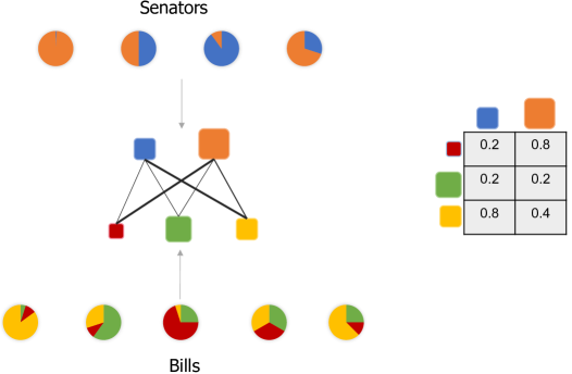
We use a probabilistic model to account for the weights of these latent community memberships. Figure 4 presents a schematic representation of our model where different colors in piecharts represent the relative likelihoods of four senators belonging to corresponding two communities (blue and orange). The same idea applies to bills, which might tap into different sets of communities of senators when attracting cosponsorships (each of five bills belonging to a mixture of three communities, represented by red, green, and yellow). These constitute the “mixed-membership” portion of the model. These mixed-memberships can be modeled using node-level covariates such as the characteristics of senators and the contents of bills.
In Figure 4, the matrix represents the stochastic block model based on the probability of forming an edge (i.e., cosponsorship) between a community of senators and that of bills. Some pairs of communities have a higher probability of cosponsorship (e.g., orange group of senators and red group of bills) than others (e.g., blue group of senators and green group of bills). These probabilities can be modeled as a function of dyadic covariates such as the indicator variable of whether or not the potential cosponsor belongs to the same Senate committee as the one, from which the bill originated.
3.2 The Bipartite Mixed-Membership Stochastic Blockmodel
We now formally present our model. Let represent a bipartite graph where and denote the two disjoint families of nodes, i.e., , and represents the set of undirected edges between two nodes of different families. Suppose that family 1 has nodes whereas the number of nodes in family 2 is . For each dyad, we let denote the latent group that node of family 1 instantiates when interacting with node of family 2 whose latent group membership is denoted by . Further, we use to denote the existence of an edge between these two nodes while indicates its absence.
We assume that the probability of edge formation is a function of a blockmodel (i.e., a matrix representing the log odds of forming an edge between any two latent group members, as illustrated by specific pairs of block colors in Figure 4) and dyadic predictors ,
| (1) |
where denotes a vector of dyad-level regression coefficients. By including a set of dyadic predictors, the model allows edge formation probabilities to be different even for pairs of nodes that have instantiated the same latent groups, thus relaxing the common assumption of stochastic equivalence. Substantively, this allows for scenarios where senator-bill dyads, whose respective nodes sort into the same pairs of latent communities, can be further differentiated in cosponsorship likelihood by characteristics pertinent to the particular dyad — such as a senator’s collaborative history with the author of the bill.
As is common in mixed-membership SBMs, we define a categorical sampling model for the dyad-specific group memberships, and , so that
| (2) |
where the probability that node of family 1 (node of family 2) instantiates a group on any possible interaction is given by () — a -dimensional (-dimensional) probability vector usually known as the mixed-membership (represented as the pie charts for each node in Figure 4).
Furthermore, our model goes beyond this standard formulation by incorporating node-level information. This is a critical feature of the model because it incorporates (monadic) senator and bill level predictor information directly into the definition of the mixed-membership probabilities of latent groups. These covariates themselves affect the cosponsorship likelihood through the resulting instantiated element of the blockmodel. Specifically, we assume that the mixed-membership probability vectors are generated according to a Dirichlet distribution with concentration parameters that are a function of node covariates,
| (3) |
where hyper-parameter vectors and contain regression coefficients associated with the th and th groups of vertex families 1 and 2, respectively.
Putting it all together, the full joint distribution of data and latent variables in our model is given by,
| (4) |
We present a plate diagram of the proposed full model in Figure A.1 of Appendix A.2, with plates delineating the (dual) monadic and dyadic portions of the data generating process.
This specification allows us to more formally describe the potential issues raised by aggregation illustrated informally on Section 2.3. A typical aggregation strategy simply sums the number of connections to a member of family shared by two members of family , which can be obtained by defining an aggregated sociomatrix . Under this aggregation strategy, and in the absence of dyadic covariates, the model in Equation (4) implies
| (5) |
where is a matrix that stacks mixed memberships for all , and similarly for . The root of the issue is that the terms in brackets in Equation (5) (i.e., the blockmodel and the mixed-memberships of Family ) are not separately identified from the aggregated sociomatrix , thus resulting in the kind of observational equivalence illustrated in Figure 2. As a result, relationships between members of Family can be misinterpreted if we rely on the aggregated data. Our model prevents this possibility by focusing on modeling the original bipartite network directly.
3.3 Estimation
With the thousands of vertices and millions of potential edges involved in an application such as bill cosponsorships, sampling directly from the posterior distribution given in Equation (4) is computationally prohibitive. To obtain estimates of quantities of interest in a reasonable amount of time, we follow the computational strategy of [40] by first marginalizing latent variables and then defining a stochastic variational approximation to the full posterior. We briefly summarize these computational strategies here.
Marginalization.
At first, and given their high dimensionality, marginalizing out dyad-specific group memberships (i.e. and ) may seem attractive. Doing so, however, would result in variational updates that cannot be computed in closed-form, as the Dirichlet-distributed mixed-membership vectors are not conjugate with respect to the Bernoulli likelihood we have adopted. Instead, we collapse the full posterior over the mixed-membership vectors (i.e. and ):
| (6) |
where is the Gamma function, , (and similarly for and ), and is a count statistic representing the number of times node instantiates group across its interactions with nodes in family 2 (and similarly for ). Lastly, is the probability of a tie between the vertices in dyad .
Using this collapsed posterior allows us to retain the ability to derive closed-form updates for the variational parameters as shown below. It has been shown that this type of marginalization scheme improves the quality of the variational approximation in other contexts [48]. We now turn to the discussion of this variational approximation.
Stochastic Variational Approximation.
To approximate the collapsed posterior proportional to Equation (6), we first define a factorized distribution of the joint dyad-specific latent group membership variables (i.e. and ) as follows:
| (7) |
where are sum-to-one, ()-dimensional variational parameters.
The goal of variational inference is to find, in the space of functions of the form given by Equation (7), one that closely approximates (in KL divergence terms) the target posterior. This is equivalent to maximizing the evidence lower bound of Equation (6) with respect to vectors :
| (8) | ||||
where is the expected value of the marginal count under the variational distribution (and similarly for ). The approximation in the last line results from using a zero-order Taylor series expansion of the expectation in place of calculating the computationally expensive integral over the Poisson-Binomial distribution of the count statistics.
In turn, we take an empirical Bayes approach and maximize the lower bound to obtain values of relevant hyper-parameters , and . After appropriate initialization (see Appendix A.4 for details), optimization of the lower bound proceeds iteratively by first updating the variational parameters according to Equation (8) (the E-step), and maximizing w.r.t. to the hyper-parameters, holding (and derived global counts and ) constant at their most recent value (the M-step), until the change in the lower bound is below a user-specified tolerance. As there are no closed-form solution for these optimal values, we rely on a numerical optimization routine (see Appendix A.3.2 for the required gradients).
We obtain measures of uncertainty around regression coefficients and by evaluating the curvature of the lower bound at the estimated optimal values for these hyper-parameters. When considering terms that involve these hyper-parameters, the lower bound reduces to the expected value of the log-posterior taken with respect to the variational distribution . As a result, evaluating the Hessian of the lower bound (and the corresponding covariance matrix of the hyper-parameters) requires evaluating that expectation. Details of the required Hessian can be found in Appendix A.5
To further improve the scalability of our variational EM approach, we rely on stochastic optimization to find a maximum of the lower bound [24, 13, 11]. Stochastic optimization follows, with decreasing step sizes, a noisy estimate of the gradient of formed by subsampling dyads in the original network. Provided the schedule of step sizes satisfies the Robbins-Monro conditions, and the gradient estimate is unbiased, the procedure is guaranteed to find a local optimum of the variational target [24], while using a fraction of the available data at each iteration.
Details of our exact procedure, including a description of how we sample dyads to form the sub-network on which gradient estimates are based, can be found in Appendix A.3.3. In turn, Appendix A.6 contains results of a simulation exercise in which we evaluate the performance of our estimation approach with respect to the accuracy of the mixed-membership estimation, the ability of the model’s predictions to reflect structural features of networks it is fit to, and the properties of our uncertainty approximation strategy.
4 Empirical Analysis
As we have seen in Section 2, a standard analysis of the aggregated cosponsorship network during the 107th Senate reveals little information beyond what is conveyed by senator partisanship. In particular, no insight is gained about what allowed this Senate to remain legislatively active, avoiding the stalemate that many associate with partisan divisions. The goal of our empirical analysis, therefore, is to uncover other relationships that help explain the extent of legislative collaboration in such divided times by applyign the proposed biMMSBM model. The model identifies the important role of junior, bipartisan power brokers, as well as the common ground they were able to establish by supporting both popular social programs and low-stakes resolutions on controversial issue areas.
4.1 Model specification
A rich literature on collaboration in Congress suggests that legislators cosponsor through partisanship, seniority, and personal political history [45, 5]. Accordingly, we include senators’ party affiliation, ideology, seniority and sex in our model as monadic predictors for how senators sort into latent communities. [22] articulates that preferences for certain types of colleagues also drive cosponsorship behavior—senators are more likely to cosponsor bills when they share closer preferences with the sponsor of the bill, and when they are more connected to their colleagues.
To capture this, we model legislation groups as a function of sponsors’ party, ideology, seniority and sex (we remove dyads for which senators are the sponsors of bills in question). Lastly, senators tend to cosponsor bills that cover specific policy domains [22]. This inclination cannot be modeled in a senator-only unipartite network, but can be directly accounted for when modeling the bipartite structure. We address this possibility by including the substantive topic of the bill as a bill-level covariate.
To capture the described shifts in the temporal context in which bills are introduced, we also include a bill-level (i.e., monadic) covariate indicating whether a bill was presented in the first phase of the Congress (prior to Jeffords leaving the Republican party), in the second phase (post Jeffords leaving the party and prior to 9/11) or in the third phase (after 9/11). The context under which a piece of legislation is introduced is an additional example of information that would inevitably be discarded in a projected unipartite analysis of the bipartite network.
Another important aspect to cosponsoring is reciprocity behaviors, or favor-trading on the Senate floor [4]. The model therefore includes a dyadic predictor measuring, for each senator-bill dyad, the (log) proportion of times the current bill’s sponsor in turn cosponsored bills introduced by the senator in the previous Congress. As this proportion of reciprocity is left-skewed with more zeroes, we include a dummy measure for whether reciprocity is zero, as well as a log proportion of reciprocity variable.333The latter variable codes log proportion of reciprocity zero values as zero, and otherwise takes logs of proportion of reciprocity directly.
Finally, our dyadic model also includes the number of committees shared by a senator and a piece of legislation. A greater number of shared committees indicates a higher chance that the senator has overseen the development of a bill and holds relevant substantive expertise. While the roles of committees have been studied previously [43, 8], our analysis directly examines how overlap in committees between legislator and legislation relates to cosponsorship. Relatedly, [19] find evidence of strong predictive power of shared committee leadership among the subset of ranking legislators when exploring cosponsorship decisions.
With predictors at the monadic and dyadic levels in place, we determine the number of latent groups for senators and bills. To do this, we first subset 20% of the data as a test set, and compare models with a range of possible latent group-size pairings through out-of-sample area under the ROC curve (AUROC) values. We then select the group sizes offering the best fit according to this AUROC criterion, resulting in 3 groups each for legislators and bills, i.e., .
After obtaining estimates for all parameters and hyper-parameters in Equation (4) for this model fit to the bipartite cosponsorship network in the 107th Senate, we compute quantities of interest in the form of predicted probabilities of block interactions and block memberships. As our discussion hinges on these derived quantities, we present all estimated values in Tables A.7 and A.8 in the Appendix.
4.2 Drivers of legislative collaboration
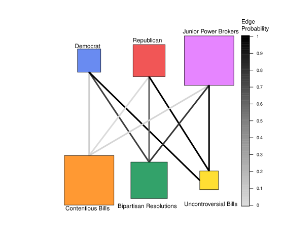
Figure 5 presents the estimated blockmodel for the 107th Senate, showing the likelihood that any two members of a senator and legislation latent group will have a tie between them. Edges in this graph are shaded by the probability that two senator-and-bill latent groups have a cosponsorship tie connecting them, while nodes are sized proportional to the expected number of times groups are instantiated across dyads.
As expected, there are estimated senator groups (depicted as the top row of squares in Figure 5) that align well with party memberships, and are thus labeled accordingly. Members of these partisan groups include Republican stalwarts (such as Strom Thurmond (R-SC) and Jesse Helms (R-NC), in the group depicted in red), and seasoned Democrats (like Robert Byrd (D-WV) and Edward Kennedy (D-MA), in the group depicted in blue). In addition, however, our model identifies a substantial group of senators (depicted in purple) who stand out as having different cosponsorship patterns than their more partisan counterparts. Exemplars of this group, whom we call the junior power brokers, include Jon Corzine (D-NJ), Tom Carper (D-DE), Susan Collins (R-ME), Bill Frist (R-TN), Zell Miller (D-GA), and Hillary Clinton (D-NC) — all junior Senators at the time. The top 10 members of each senator latent group by mixed membership probability are presented in Table A.5 in the Appendix.
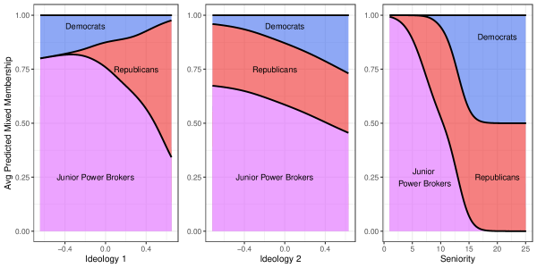
Indeed, this third, bipartisan group is likely to be formed by senators who have little experience in the Senate coming from all over the ideological spectrum.444The plotted quantities are obtained by computing , where the expectation is taken over the observed values of all but a focal variable (e.g., ideology), and the are estimated monadic coefficients. A full table of estimates of monadic coefficients can be found in Table A.8 in the Appendix. This is indicated by the left-most panel of Figure 6, which shows how the probability of group membership changes as a function of ideology. Although this group of junior power brokers is primarily comprised of left-leaners on the first DW-Nominate dimension, positions along the second ideological dimension (as seen in the central panel of the figure) — often interpreted as capturing cross-cutting salient issues of the day [42] — help distinguish this group of senators from their staunch Democrat counterparts. Many of these junior power brokers (whom can be inspected in Table A.5 of the Appendix) later became new leadership in their respective parties,555For example, as the end of the 107th Congress drew near, the Senate Republican Conference saw some leadership changes; importantly, Trent Lott lost substantial support among conservatives and was sharply reprimanded by Democrats over racist remarks he made at Strom Thurmand’s 100th birthday. He was forced to step down and was quickly replaced with the much more junior Bill Frist (R-TN), who was a heart surgeon with a strong platform on healthcare issues and seen as less likely to delve into sticky race issues. or were pivotal “last” votes in large contentious bills that required just an extra nudge or two for passage.666For instance, a major bill in the 107th was the Farm Bill, designed to repeal the Freedom to Farm Act of 1996. While politics over agriculture had historically been regional rather than ideological, the Freedom to Farm Act had been a significant deviation from that norm. Veteran senators Tom Daschle (D-SD) and Agriculture Committee Chairman Tom Harkin (D-IA) collaborated to bring the Farm Bill together, and a series of negotiations began to bring the necessary senatorial support on board — including support for small dairy farmers included in the bill. In the end, the largely Democratic set of supporters was complemented by key support from relatively junior Republicans Susan Collins (R-ME) and Jeff Sessions (R-AL). This role as brokers is further supported by analyses of the betweeness centrality777Betweeness centrality measures, for each node, the number of shortest paths that include it — effectively giving us a sense of the extent that a node serves as a “bridge” when connecting any two other nodes in the network, and thus a sense of how often nodes can broker relationships in the network. of Senators who are likely to instantiate this group, which tends to be higher than that of Senators whose membership in the other two groups is more likely (see Table A.9 in the Appendix).
Furthermore, the model is able to identify the types of legislation that these groups of senators are likely to cosponsor (or not). In this case, the model uncovers three broad classes of bills and resolutions (depicted in the bottom row of squares in Figure 5), as well as the corresponding probabilities that members of any of the three senator groups will support them through cosponsorship decisions. We next show that investigating the characteristics of these groups can further help us understand how collaboration in the form of cosponsorships happened during this session of Congress.
4.3 Legislation types affect cosponsorship
The largest type of legislation uncovered by our model is also the least likely to be supported by members of any senator group, suggesting that the bulk of legislation introduced in the Senate received little support from Senators other than the original sponsor. This latent class of bills, which we labeled “Contentious Issues” in Figure 5, consists of high-stakes bills on controversial economic issues and social programs, including those bills that handle the allocation of public funds for such programs. For example, the Senior Self-Sufficiency Act (SN 107 2842), and the Bioterrorism Awareness Act (SN 107 1548), and the Nationwide Health Tracking Act of 2002 (SN 107 2054) belong to this group. Table A.6 in the Appendix presents details of legislation with the top ten mixed membership probabilities in each of the three latent groups.888The group is also very likely to contain legislation that was introduced by junior Democrat women — especially during the last phase of this Senate session. Indeed, for the top one hundred pieces of legislation with highest mixed memberships in this group, all are Democrats, and 96 are female. Although the larger volume of legislation introduced by female Democratic Senators is not surprising (the 107th was also noteworthy for re-invigorating the trend in female membership started in 1992, during the so-called “Year of Woman”), the lack of support elicited by such efforts invites further examination. We leave this for future research.
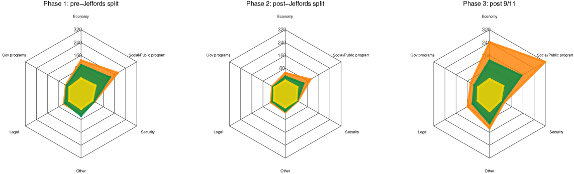

The size of the “Contentious Bills” group grew during the third and last phase of the 107th Senate, after the attacks in 9/11. This can be easily seen in Figure 7, which presents radar plots of predicted legislation memberships by phase of the Congress (panels from left to right present bills from the pre-Jeffords’ split phase, post-Jeffords’ split second phase, and post 9/11 phase, in turn). Each radar graph positions the six possible substantive topics at a vertex of the hexagon, and plots the predicted number of bills in each topic by latent group (using shaded polygons).999The polygons are obtained by summing each latent group’s estimated mixed membership proportions for a given topic in a single phase—a way to think of bills in each group allocated towards each topic—and plotting these against each topic pole’s total number of bills. The dominance of bills in the “Contentious Bills” group in the third phase, depicted in orange, is readily apparent.
How, then, were the different senator groups able to find common ground in order to avoid stalemate? Clues can be found in the definition of the other two latent bill groups uncovered by our model — the groups we have labeled “Bipartisan Resolutions” and “Popular & Uncontroversial” in both Figures 5 and 7. The former is particularly illuminating: its topical composition almost mirrors that of the “Contentious Bills” (i.e., it is comprised of pieces of legislation that deal with controversial public social programs and economic issues, as indicated by the similar shapes of green and orange polygons in Figure 7), but it is likely to be comprised of resolutions, rather than bills, thus offering lower-stakes opportunities for presenting bipartisan positions that do not result in codified law.101010Although joint resolutions carry the same weight of bills, in the sense that they could also ultimately become law, many joint resolutions are either just as symbolic as their concurrent or simple counterparts (e.g., constitutional amendments are extremely difficult to ratify) or deal with less permanent matters (e.g., extending appropriation levels until the appropriate bill is passed) than actual bills. Thus, we typically refer to them as “low-stakes” opportunities for bipartisan work. Such resolutions, which tend to be sponsored by more senior members (such as SJ 107 4, sponsored by Fritz Hollings (D-SC), which proposed a constitutional amendment to regulate campaign expenditures; see Table A.6 of the Appendix for more such examples), offer opportunities to build bridges across partisan and experience divides without incurring the costs associated with creating laws.
In turn, members of the comparatively smaller “Popular & Uncontroversial” pieces of legislation (shown in yellow in Figures 5 and 7) also draw consistent cosponsorship support from all senator groups, as members tend to be either uncontroversial resolutions or bills on popular social programs. As a result, such legislation is widely cosponsored by Republicans and Democrats alike. For instance, the Senate joint resolution over the Sept. 11 attacks (SJ 107 22) has the highest mixed membership probability in this group, followed closely by bills such as the Railroad Retirement and Survivors’ Improvement Act of 2001 (SN 107 697). Such bills and resolutions form a small but steady core of legislation that supplements low-stakes efforts (such as those in the “Bipartisan Resolutions” block), that can nevertheless result in substantial legislation, such as the Family Opportunity Act of 2002 (SN 107 321).
Overall, Senators appear to have leveraged a mix of low-stakes resolutions over potentially contentious issues and a small set of legislation over which there was bipartisan support in order to build cross-partisan bridges and keep the 107th session from devolving into stalemate. Our model identified these patterns after accounting for the forces that have been found to drive collaboration through cosponsorship.
In particular, the blockmodel structure we found was net of two important drivers of cosponsorship likelihood quid pro quo behaviors (represented by dyadic predictors), measured as the coefficient on the (log) proportion of “reciprocity” (Log Reciprocity), and the shared committee experience of a given senator-bill dyad (Shared Committee). In the case of the former, our model suggests that a 1% increase in the reciprocity (i.e., the proportion of times the sponsor of a piece of legislation acted as a cosponsor for a given senator’s bill in the previous Congress) is associated with a 2% increase in the likelihood of cosponsorship. In the case of the latter, we find that sharing a committee is significantly and positively associated with collaboration, making cosponsorship about 3 times more likely. These results, which can be fully explored in Table A.7 in the Appendix, are consistent with previous research on the determinants of legislative collaboration — lending further credence to our general findings.
5 Conclusion
We have developed a new approach to modeling bipartite networks that allows researchers to incorporate more complete information available to them, without the need to incur losses stemming from relevant data aggregation. We extend the mixed-membership network model to two-mode networks with distinct community structures, and incorporate monadic and dyadic predictors into the standard blockmodel specification. Our proposed model, therefore, allows applied researchers to evaluate hypotheses about affiliation network formation and to make link predictions for previously unobserved dyads.
Using data connecting legislators and bills through cosponsorship decisions made during the 107th U.S. Senate, we illustrate our model’s ability to recover both familiar patterns and to discover novel regularities in the process that results in observed cosponsorship networks. Specifically, while we find evidence of partisan preferential attachment as a driving force in the definition of cosponsorship ties, we also establish the importance of junior legislators who have the power to broker deals across the aisle.
We find the kinds of legislation that allowed members of the 107th Senate to remain productive in spite of stark partisan divisions. A focus on a small set of bills and resolutions over which bipartisan agreement could be found, paired with a set of mostly symbolic resolutions on more controversial topics, provided the common ground needed avoid substantial gridlock. As such, our model uncovers lessons that are relevant to understanding of the possibilities in today’s similarly divided Senate: an emphasis on the importance of junior legislators (who have proven to be as much as source of division today as they were a force for collaboration during the 107th Senate), as well as the opportunities afforded by the small set of legislation – and particularly, resolutions — over which bipartisan agreement can be found.
Our approach allows us to directly explore hypotheses that would have been obscured by the commonly employed projection of the bipartite network onto a univariate network, uncovering direct evidence that shows the value of reciprocity in legislative activity. As bipartite networks are quite common in the social sciences, we see natural applications of our model to gaining purchase on a diversity of questions relating to — among others — country-trade product networks, state memberships in organizations, Twitter discussions and hashtags, or product recommender systems.
In the future, and given the prevalence of networks observed over time, fruitful extensions of our proposed approach would allow researchers to incorporate dynamics into the generative model of bipartite network formation [40, for an extension incorporating dynamics in the unipartite case, see]. Such an extension would make forecasting network ties possible even in the absence of other predictors, and it would enable researchers to use the vast amounts of data available in time-stamped two-mode networks.
Another future extension would be to allow for networks of even larger numbers of node-types — allowing, for instance, the incorporation of lobbying firms into the cosponsorship network, or the study of NGOs, IGOs and countries in the international system. Such multi-mode networks can offer alternative ways of conducting co-clustering of multiple actors who are embedded in common networks, but whose connections are indirect. The prevalence of such types of connections warrants the development of more and better tools to study relational data that do not conform to the traditional single-mode network representation, offering alternatives that do not succumb to aggregation bias.
References
- [1] Edoardo Maria Airoldi, David M Blei, Stephen E Fienberg and Eric P Xing “Mixed membership stochastic blockmodels” In Journal of machine learning research, 2008
- [2] Laura W. Arnold, Rebecca E. Deen and Samuel C. Patterson “Friendship and Votes: The Impact of Interpersonal Ties on Legislative Decision Making” In State and Local Government Review 32.2, 2000, pp. 142–147 DOI: 10.1177/0160323X0003200206
- [3] Marco Battaglini, Valerio Leone Sciabolazza and Eleonora Patacchini “Effectiveness of connected legislators” In American Journal of Political Science 64.4 Wiley Online Library, 2020, pp. 739–756
- [4] Laurence Brandenberger “Trading favors—Examining the temporal dynamics of reciprocity in congressional collaborations using relational event models” In Social Networks 54, 2018, pp. 238–253 DOI: 10.1016/j.socnet.2018.02.001
- [5] Kathleen A. Bratton and Stella M. Rouse “Networks in the Legislative Arena: How Group Dynamics Affect Cosponsorship” In Legislative Studies Quarterly 36.3, 2011, pp. 423–460 DOI: 10.1111/j.1939-9162.2011.00021.x
- [6] James E Campbell “Cosponsoring legislation in the US Congress” In Legislative Studies Quarterly JSTOR, 1982, pp. 415–422
- [7] Xun Cao “Networks of intergovernmental organizations and convergence in domestic economic policies” In International Studies Quarterly 53.4 Blackwell Publishing Ltd Oxford, UK, 2009, pp. 1095–1130
- [8] Alexandra Cirone and Brenda Van Coppenolle “Cabinets, Committees, and Careers: The Causal Effect of Committee Service” In The Journal of Politics 80.3, 2018, pp. 948–963 DOI: 10.1086/697252
- [9] Bruce A Desmarais and Skyler J Cranmer “Statistical inference for valued-edge networks: The generalized exponential random graph model” In PloS one 7.1 Public Library of Science San Francisco, USA, 2012, pp. e30136
- [10] Bruce A Desmarais, Jeffrey J Harden and Frederick J Boehmke “Persistent policy pathways: Inferring diffusion networks in the American states” In American Political Science Review 109.2 Cambridge University Press, 2015, pp. 392–406
- [11] Adrien Dulac, Eric Gaussier and Christine Largeron “Mixed-Membership Stochastic Block Models for Weighted Networks” In Conference on Uncertainty in Artificial Intelligence, 2020, pp. 679–688 PMLR
- [12] Christian Fong “Expertise, networks, and interpersonal influence in congress” In The Journal of Politics 82.1 The University of Chicago Press Chicago, IL, 2020, pp. 269–284
- [13] James Foulds, Levi Boyles, Christopher DuBois, Padhraic Smyth and Max Welling “Stochastic collapsed variational Bayesian inference for latent Dirichlet allocation” In Proceedings of the 19th ACM SIGKDD international conference on Knowledge discovery and data mining, 2013, pp. 446–454
- [14] James H. Fowler “Connecting the Congress: A Study of Cosponsorship Networks” In Political Analysis 14.4 Cambridge University Press, 2006, pp. 456–487 DOI: 10.1093/pan/mpl002
- [15] James H. Fowler “Legislative cosponsorship networks in the US House and Senate” In Social Networks 28.4, 2006, pp. 454–465
- [16] Ove Frank and David Strauss “Markov graphs” In Journal of the american Statistical association 81.395 Taylor & Francis, 1986, pp. 832–842
- [17] Prem K Gopalan and David M Blei “Efficient discovery of overlapping communities in massive networks” In Proceedings of the National Academy of Sciences 110.36 National Acad Sciences, 2013, pp. 14534–14539
- [18] Gérard Govaert and Mohamed Nadif “Clustering with block mixture models” In Pattern Recognition 36.2, 2003, pp. 463–473 DOI: 10.1016/S0031-3203(02)00074-2
- [19] Justin H. Gross and Justin Kirkland “Rivals or Allies? A Multilevel Analysis of Cosponsorship within State Delegations in the US Senate” In Congress & the Presidency 46.2 Taylor & Francis, 2019, pp. 183–213
- [20] Matt Grossmann and Kurt Pyle “Lobbying and congressional bill advancement” In Interest Groups & Advocacy 2.1 Springer, 2013, pp. 91–111
- [21] Mark S Handcock, Adrian E Raftery and Jeremy M Tantrum “Model-based clustering for social networks” In Journal of the Royal Statistical Society: Series A (Statistics in Society) 170.2 Wiley Online Library, 2007, pp. 301–354
- [22] Brian M. Harward and Kenneth W. Moffett “The Calculus of Cosponsorship in the U.S. Senate” In Legislative Studies Quarterly 35.1, 2010, pp. 117–143 DOI: https://doi.org/10.3162/036298010790821950
- [23] Peter D Hoff, Adrian E Raftery and Mark S Handcock “Latent space approaches to social network analysis” In Journal of the american Statistical association 97.460 Taylor & Francis, 2002, pp. 1090–1098
- [24] Matthew D Hoffman, David M Blei, Chong Wang and John Paisley “Stochastic variational inference” In The Journal of Machine Learning Research 14.1 JMLR. org, 2013, pp. 1303–1347
- [25] Zan Huang, Xin Li and Hsinchun Chen “Link prediction approach to collaborative filtering” In Proceedings of the 5th ACM/IEEE-CS Joint Conference on Digital Libraries (JCDL’05), 2005, pp. 141–142 IEEE
- [26] David R Hunter, Steven M Goodreau and Mark S Handcock “Goodness of fit of social network models” In Journal of the american statistical association 103.481 Taylor & Francis, 2008, pp. 248–258
- [27] Brian Karrer and Mark EJ Newman “Stochastic blockmodels and community structure in networks” In Physical review E 83.1 APS, 2011, pp. 016107
- [28] In Song Kim and Dmitriy Kunisky “Mapping Political Communities: A Statistical Analysis of Lobbying Networks in Legislative Politics” In Political Analysis Cambridge University Press, 2020, pp. 1–20 DOI: 10.1017/pan.2020.29
- [29] In Song Kim, Steven Liao and Kosuke Imai “Measuring Trade Profile with Granular Product-Level Data” In American Journal of Political Science 64.1 Wiley Online Library, 2020, pp. 102–117
- [30] Justin H. Kirkland “The Relational Determinants of Legislative Outcomes: Strong and Weak Ties Between Legislators” In The Journal of Politics 73.3, 2011, pp. 887–898 DOI: 10.1017/S0022381611000533
- [31] Glen S. Krutz “Issues and Institutions: ”Winnowing” in the U.S. Congress” In American Journal of Political Science 49.2, 2005, pp. 313–326 DOI: 10.1111/j.0092-5853.2005.00125.x
- [32] Andrea Lancichinetti, M Irmak Sirer, Jane X Wang, Daniel Acuna, Konrad Körding and Luı́s A Nunes Amaral “High-reproducibility and high-accuracy method for automated topic classification” In Physical Review X 5.1 APS, 2015, pp. 011007
- [33] Daniel B. Larremore, Aaron Clauset and Abigail Z. Jacobs “Efficiently inferring community structure in bipartite networks” In Physical Review E 90.1, 2014, pp. 012805 DOI: 10.1103/PhysRevE.90.012805
- [34] Jennifer M Larson “Networks and interethnic cooperation” In The Journal of Politics 79.2 University of Chicago Press Chicago, IL, 2017, pp. 546–559
- [35] Jennifer L. Lawless, Sean M. Theriault and Samantha Guthrie “Nice Girls? Sex, Collegiality, and Bipartisan Cooperation in the US Congress” In The Journal of Politics 80.4, 2018, pp. 1268–1282 DOI: 10.1086/698884
- [36] Zeev Maoz, Ranan D Kuperman, Lesley Terris and Ilan Talmud “Structural equivalence and international conflict: A social networks analysis” In Journal of Conflict Resolution 50.5 Sage Publications Sage CA: Thousand Oaks, CA, 2006, pp. 664–689
- [37] Shahryar Minhas, Peter D Hoff and Michael D Ward “Inferential approaches for network analysis: Amen for latent factor models” In Political Analysis 27.2 Cambridge University Press, 2019, pp. 208–222
- [38] Taishi Muraoka “The Cosponsorship Patterns of Reserved Seat Legislators” In Legislative Studies Quarterly 45.4 Wiley Online Library, 2020, pp. 555–580
- [39] Santiago Olivella, Adeline Lo, Tyler Pratt and Kosuke Imai “NetMix: Dynamic Mixed-Membership Network Regression Model” R package version 0.2.0.9013, 2021 URL: https://CRAN.R-project.org/package=NetMix
- [40] Santiago Olivella, Tyler Pratt and Kosuke Imai “Dynamic Stochastic Blockmodel Regression for Social Networks: Application to International Conflicts” In Journal of the American Statistical Association 117.539, 2022, pp. 1068–1081
- [41] Tiago P Peixoto “Hierarchical block structures and high-resolution model selection in large networks” In Physical Review X 4.1 APS, 2014, pp. 011047
- [42] Keith T Poole and Howard Rosenthal “Ideology & congress: A political economic history of roll call voting” Routledge, 2017
- [43] Mason A. Porter, Peter J. Mucha, M… Newman and Casey M. Warmbrand “A network analysis of committees in the U.S. House of Representatives” In Proceedings of the National Academy of Sciences 102.20, 2005, pp. 7057–7062
- [44] Zahra S. Razaee, Arash A. Amini and Jingyi Jessica Li “Matched Bipartite Block Model with Covariates” In Journal of Machine Learning Research 20.34, 2019, pp. 1–44 URL: http://jmlr.org/papers/v20/17-153.html
- [45] Paulina S. Rippere “Polarization Reconsidered: Bipartisan Cooperation through Bill Cosponsorship” In Polity 48.2, 2016, pp. 243–278 DOI: 10.1057/pol.2016.4
- [46] Stewart “Congressional Committee Assignments, 103rd to 114th Congresses, 1993–2017: Senate Committee Assignment Data, updated 11/17/2017” In Charles Stewart’s Congressional Data Page, 2020 URL: http://web.mit.edu/17.251/www/data_page.html#1
- [47] Wendy K. Tam Cho and James H. Fowler “Legislative Success in a Small World: Social Network Analysis and the Dynamics of Congressional Legislation” In The Journal of Politics 72.1, 2010, pp. 124–135 DOI: 10.1017/S002238160999051X
- [48] Yee W. Teh, David Newman and Max Welling “A Collapsed Variational Bayesian Inference Algorithm for Latent Dirichlet Allocation”, 2007
- [49] Stanley Wasserman and Philippa Pattison “Logit models and logistic regressions for social networks: I. An introduction to Markov graphs andp” In Psychometrika 61.3 Springer, 1996, pp. 401–425
- [50] Arthur White and Thomas Brendan Murphy “Mixed-membership of experts stochastic blockmodel” In Network Science 4.1 Cambridge University Press, 2016, pp. 48–80
- [51] Yan Zhang, Andrew J Friend, Amanda L Traud, Mason A Porter, James H Fowler and Peter J Mucha “Community structure in Congressional cosponsorship networks” In Physica A: Statistical Mechanics and its Applications 387.7, 2008, pp. 1705–1712
- [52] Zhixin Zhou and Arash A. Amini “Analysis of spectral clustering algorithms for community detection: the general bipartite setting” In Journal of Machine Learning Research 20.47, 2019, pp. 1–47 URL: http://jmlr.org/papers/v20/18-170.html
Appendix A Appendix
A.1 Projecting Bipartite Networks onto Unipartite Networks is a Common Practice
| Author | Journal | Network | Projected |
| Alliances | |||
| Maoz (2009) | AJPS | alliances and trade network | Yes |
| Franzese Hays & Kachi (2012) | PA | alliances across countries | Yes |
| Kinne & Bunte (2018) | BJPS | defense cooperation agreements network | Yes |
| Communication | |||
| Aarøe & Peterson (2018) | BJPS | media flows | Yes |
| Boucher & Thies (2019) | JOP | Yes | |
| Siegel & Badaan (2020) | APSR | Yes | |
| Conflict | |||
| Cranmer & Desmarais (2011) | PA | legislative cosponsorship, conflict | Yes |
| Rozenas, Minhas & Ahlquist (2019) | PA | conflict and treaty network | Yes |
| Nieman et al. (2021) | JOP | troop placement network | Yes |
| Congress & Parliament | |||
| Cho & Fowler (2010) | JOP | legislative cosponsorship | Yes |
| Maoz & Somer-Topcu (2010) | BJPS | European parliamentary parties and cabinets | Yes |
| Malang, Brandenberger & Leifeld (2017) | BJPS | European legislative proposals and parliaments | No |
| Box-Steffensmeier et al. (2018) | AJPS | Dear Colleague letters | Yes |
| Zelizer (2019) | APSR | cue taking for policy position taking in legislature | Yes |
| Battaglini, Sciabolazza & Patacchini (2020) | AJPS | legislative cosponsorship | Yes |
| Kim & Kunisky (2020) | PA | Congressional lobbying | No |
| International organizations | |||
| Martinsen, Schrama & Mastenbroeck (2020) | BJPS | welfare governance network | Yes |
| International political economy | |||
| Bodea & Hicks (2015) | JOP | central bank independence for countries and firms | Yes |
| Kim, Liao & Imai (2019) | AJPS | trade network | Yes |
| Policies | |||
| Desmarais, Harden & Boehmke (2015) | APSR | policy adoption across states | Yes |
| Fischer & Sciarini (2016) | JOP | policy collaboration across sectors | Yes |
| Gilardi, Shipan & Wuest (2020) | AJPS | policy adoption, issue definition | Yes |
| Political elites | |||
| Nyhan & Montgomery (2015) | AJPS | campaign consultants | Yes |
| Pietryka & Debats (2017) | APSR | voters and elites | Yes |
| Weschle (2017) | BJPS | party relationships with societal groups | Yes |
| Weschle (2018) | APSR | political and social actors | Yes |
| Jiang & Zeng (2019) | JOP | elite network | Yes |
| Box-Steffensmeier et al. (2020) | AJPS | campaign donor list sharing | Yes |
| Village networks | |||
| Larson (2017) | JOP | ethnic cooperation | Yes |
| Haim, Nanes & Davidson (2021) | JOP | police community connections | Yes |
A.2 Plate Diagram of the Proposed Model
A.3 Details of the Variational EM Algorithm
A.3.1 E-step
E-step: and
Variational parameters are updated by restricting Equation (8) to terms that depend only on and and taking the logarithm of the resulting expression,
Now, note that and that, for , . Since the , we can re-express and thus simplify the expression to,
Then take the expectation under the variational distribution :
The exponential of this expression corresponds to the (unnormalized) parameter vector of a multinomial distribution .
The update for is similarly derived. Restrict Equation (8) to the terms that depend only on (for specific and nodes in ) and taking the logarithm of the resulting expression,
Re-express and thus simplify the expression to,
Take the expectation under the variational distribution :
A.3.2 M-step
Lower Bound
Expression for the lower bound,
M-step 1: update for
Restricting the lower bound to terms that contain (blockmodel), we obtain
Optimize this lower bound with respect to using a gradient-based numerical optimization method. The corresponding gradient is given by,
M-step 2: update for
Restricting the lower bound to terms that contain (dyadic coefficients), and recalling that , we have
To optimize this expression with respect to (the th element of the vector), we again use a numerical optimization algorithm based on the following gradient,
M-step 3: update for ,
Let , , , and . To find the optimal value of , we roll all terms not involving the coefficient vector into a constant:
No closed form solution exists for an optimum w.r.t. , but a gradient-based algorithm can be implemented to maximize the above expression. The corresponding gradient with respect to each element of is given by,
where is the digamma function. Once again, we can approximate expectations of non-linear functions of random variables using a zeroth-order Taylor series expansion. The M-step for the regression coefficients of the second family is similarly defined.
A.3.3 Stochastic variational inference
On the th iteration, our algorithm completes the following steps:
-
1.
Sample a subset of dyads , with corresponding sets of vertices and .
-
2.
Update all according to Eq. 8, and compute a set of intermediate global count statistics (after normalization),
weighted so as to match the amount of information contained in the original network.
-
3.
Update the matrices of global count statistics using an online average that follows an appropriately decreasing step-size schedule:
where step-size such that and .
-
4.
Update values of hyper-parameters by taking an “online” step in the direction of the (noisy) Euclidean gradient of w.r.t :
with appropriate gradients given in the Appendix.
Although different dyad sampling heuristics used for Step 1 can result in unbiased gradient estimates [17, see], we follow the scheme proposed by [11], which is both simple to implement and has been found to work well in sparse settings. The procedure is as follows:
-
1.
Sample a node in uniformly at random.
-
2.
Form a set (i.e., the set of all connected dyads involving ). Form sets (i.e., a set of some disconnected dyads involving ), where each set is of equal cardinality, and the disconnected dyads are sampled uniformly at random and with replacement.
-
3.
Sample, with equal probability, either or any of the sets. This set of dyads constitutes a subnetwork.
In our application, we set and set be times the number of non-links between and every other vertex in the network.
After the algorithm converges, we can easily recover the mixed-membership vectors by computing their posterior predictive expectations:
A.4 Initial values for and
Implementation of the model requires defining good starting values for the mixed-membership vectors. While spectral clustering methods offer good starting values for and in the unipartite setting, applying it to non-square affiliation matrices poses interesting challenges. To produce high-quality initial values in a viable amount of time we rely on the co-clustering approach of [18], which estimates a simpler, single-membership SBM using a fast EM algorithm.
A.5 Standard error computation
A.5.1 Hessian for
Restricted to terms that involve , the typical element of the required Hessian is given by
where is the Kronecker delta function, and the term
is a closed-form solution to the expectation over the variational distribution of the model’s parameters.
A.5.2 Hessian for and
In turn, and focusing on Family 1 coefficients, we can characterize the Hessian of the lower bound w.r.t. with
for coefficients in the same group , and
for coefficients associated with different latent groups and . As before, we use to denote the digamma function, and to denote the trigamma function.
Unlike the Hessian for , there are no closed-form solutions for the expectations involved in these expressions. To approximate them, we take samples from the Poisson-Binomial distribution of , , and let
The Hessian for the coefficients associated with Family 2, , is similarly approximated.
A.6 Simulation results
Setup.
To do so, we simulate bipartite networks with unbalanced numbers of Senator and Bills nodes under 6 different scenarios, defined by overall network size and difficulty of the mixed-membership learning problem. More specifically, we define small (i.e. 300 total nodes) and large (i.e. 3000 total nodes) networks, each with twice as many Bill nodes as there are Senator nodes. In all instances, we define the edge-generating process according to our model, using latent groups for each of the node types, a single monadic predictor drawn independently from , and a single irrelevant dyadic predictor drawn from a standard Normal distribution.
| Scenario Difficulty | Blockmodel | Monadic Coefficients |
| Easy | ||
| Medium | ||
| Hard |
To simulate different levels of estimation difficulty, we vary both the blockmodel and the coefficients associated with the mixed-membership vectors, which are set to be equal across the two node types. In the “easy” scenario, memberships are barely mixed, and there is a clear difference in edge probabilities between different groups of the different node types. In contrast, the “hard” scenario is such that all nodes have a roughly equal probability of instantiating each block, and there is little difference in the probabilities of forming edges between blocks, as given by the blockmodel. The “medium” scenario offers a more realistic, in-between estimation problem. The specific values we use in each case are given in Table A.2.
Results.
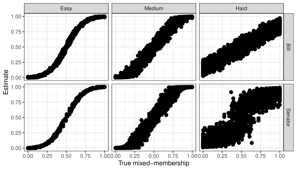
We begin by evaluating the accuracy of mixed-membership estimation by comparing true and estimated mixed-membership vectors (after re-labeling the latter to match the known, simulated group labels using the Hungarian algorithm). The correlations across node types and difficulty scenarios are demonstrated in Figure A.2. Overall, our model retrieves these mixed-membership vectors with a very high degree of accuracy — even in regimes in which block memberships play a small role in the generation of edges, and regardless of whether there is an asymmetry in the number of nodes in each family.
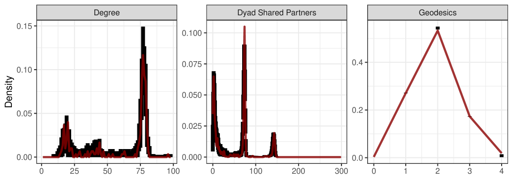
Next, we evaluate the accuracy of estimated node-level and dyadic coefficients by simulating derived quantities of interest based on them, and comparing these simulated quantities to their true counterparts, as one would when conducting a goodness-of-fit analysis based on posterior predictive distributions. As is typical in network modeling, these derived quantities are structural features of the network [26, e.g.]. Figure A.3 depicts three such features — node degree, the number of partners shared by each node dyad, and the minimum geodesic distance between nodes in the network. In each panel, the red line traces the true distribution of these network statistics, while the black vertical bars track their distribution across 100 network replicates, each generated using the estimated coefficients. If the latter are correctly estimated, network replicates should have characteristics that reflect that on which the estimation is based, and the red line should fall squarely within each vertical black rectangle. Overall, network characteristics are well recovered by our model.
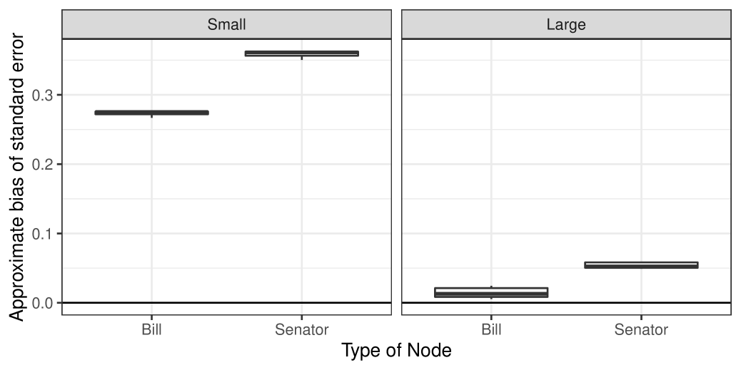
Finally, we evaluate the frequentist properties of our estimates of uncertainty in regression parameters by evaluating the extent to which they reflect the variability we can expect from repeated network sampling. To do so, we sample 100 networks from each of our 6 scenarios, for a total of 600 simulated networks. Figure A.4 shows, for each simulation scenario, the difference between our standard errors and the standard deviation across coefficients estimated on each of the network replicates. For small networks, our standard errors can be conservative — particularly for the set of coefficients associated with the smaller group of Senator nodes. As the number of nodes increases, however, our estimated uncertainty more accurately reflects the variability we would expect to see under repeated sampling.
A.7 Additional Empirical Results
A.7.1 Summarizing information for Congress 107
| Democrats | Republicans | ||
| Akaka, Daniel K. [HI] | Hollings, Ernest F. [SC] | Allard, A. Wayne [CO] | Hutchinson, Tim [AR] |
| Baucus, Max [MT] | Inouye, Daniel K. [HI] | Allen, George [VA] | Hutchison, Kay Bailey [TX] |
| Bayh, Evan [IN] | Johnson, Tim [SD] | Bennett, Robert F. [UT] | Inhofe, Jim [OK] |
| Biden Jr., Joseph R. [DE] | Kennedy, Edward M. [MA] | Bond, Christopher S. [MO] | Jeffords, James M. [VT] |
| Bingaman, Jeff [NM] | Kerry, John F. [MA] | Brownback, Sam [KS] | Kyl, Jon [AZ] |
| Boxer, Barbara [CA] | Kohl, Herb [WI] | Bunning, Jim [KY] | Lott, Trent [MS] |
| Breaux, John B. [LA] | Landrieu, Mary [LA] | Burns, Conrad R. [MT] | Lugar, Richard G. [IN] |
| Byrd, Robert C. [WV] | Leahy, Patrick J. [VT] | Campbell, Ben Nighthorse [CO] | McCain, John [AZ] |
| Cantwell, Maria [WA] | Levin, Carl [MI] | Chafee, Lincoln D. [RI] | McConnell, Mitch [KY] |
| Carnahan, Jean [MO] | Lieberman, Joseph I. [CT] | Cochran, Thad [MS] | Murkowski, Frank H. [AK] |
| Carper, Thomas R. [DE] | Lincoln, Blanche [AR] | Collins, Susan M. [ME] | Nickles, Don [OK] |
| Cleland, Max [GA] | Mikulski, Barbara A. [MD] | Craig, Larry E. [ID] | Roberts, Pat [KS] |
| Clinton, Hillary Rodham [NY] | Miller, Zell [GA] | Crapo, Michael D. [ID] | Santorum, Rick [PA] |
| Conrad, Kent [ND] | Murray, Patty [WA] | DeWine, Michael [OH] | Sessions, Jeff [AL] |
| Corzine, Jon [NJ] | Nelson, Bill [FL] | Domenici, Pete V. [NM] | Shelby, Richard C. [AL] |
| Daschle, Thomas A. [SD] | Nelson, E. Benjamin [NE] | Ensign, John E. [NV] | Smith, Bob [NH] |
| Dayton, Mark [MN] | Reed, John F. [RI] | Enzi, Michael B. [WY] | Smith, Gordon [OR] |
| Dodd, Christopher J. [CT] | Reid, Harry M. [NV] | Fitzgerald, Peter [IL] | Snowe, Olympia J. [ME] |
| Dorgan, Byron L. [ND] | Rockefeller, Jay [WV] | Frist, Bill [TN] | Specter, Arlen [PA] |
| Durbin, Richard J. [IL] | Sarbanes, Paul S. [MD] | Gramm, Phil [TX] | Stevens, Ted [AK] |
| Edwards, John [NC] | Schumer, Charles E. [NY] | Grassley, Charles E. [IA] | Thomas, Craig [WY] |
| Feingold, Russell D. [WI] | Stabenow, Debbie [MI] | Gregg, Judd [NH] | Thompson, Fred [TN] |
| Feinstein, Dianne [CA] | Torricelli, Robert G. [NJ] | Hagel, Chuck [NE] | Thurmond, Strom [SC] |
| Graham, Bob [FL] | Wellstone, Paul D. [MN] | Hatch, Orrin G. [UT] | Voinovich, George V. [OH] |
| Harkin, Tom [IA] | Wyden, Ron [OR] | Helms, Jesse [NC] | Warner, John W. [VA] |
| Concurrent resolutions | Resolutions | Joint resolutions | Bills | |
| Democrat cosponsorships | 68 | 171 | 22 | 1288 |
| Republican cosponsorships | 63 | 105 | 17 | 899 |
A.8 Model outputs
A.8.1 Group memberships
| Senior Democrats | Senior Republicans | Junior Power Brokers |
| Byrd, Robert C. [WV] | Helms, Jesse [NC] | Corzine, Jon [NJ] |
| Inouye, Daniel K. [HI] | Thurmond, Strom [SC] | Carnahan, Jean [MO] |
| Hollings, Ernest F. [SC] | Lott, Trent [MS] | Carper, Thomas R. [DE] |
| Kennedy, Edward M. [MA] | Stevens, Ted [AK] | Dayton, Mark [MN] |
| Breaux, John B. [LA] | Cochran, Thad [MS] | Miller, Zell [GA] |
| Sarbanes, Paul S. [MD] | Hatch, Orrin G. [UT] | Clinton, Hillary Rodham [NY] |
| Biden Jr., Joseph R. [DE] | Domenici, Pete V. [NM] | Bayh, Evan [IN] |
| Baucus, Max [MT] | Grassley, Charles E. [IA] | Nelson, E. Benjamin [NE] |
| Akaka, Daniel K. [HI] | Smith, Bob [NH] | Stabenow, Debbie [MI] |
| Leahy, Patrick J. [VT] | Nickles, Don [OK] | Feingold, Russell D. [WI] |
| Contentious Bills | Bipartisan Resolutions | Popular & Uncontroversial |
| SN_107_2842 Senior Self-Sufficiency Act; allocation of $1M grants to provide supportive services to elderly in noninstitutional residences. | SJ_107_1 Joint resolution proposing amendment to Constitution of US relating to voluntary school prayer. | SJ_107_22 Joint resolution expressing sense of Senate/House regarding terrorist attacks on September 11, 2001. |
| SN_107_1548 Bioterrorism Awareness Act. | SE_107_82 Resolution authorize production of records by Permanent Subcommittee on Investigations of Committee on Governmental Affairs and representation by Senate Legal Counsel. | SE_107_169 Resolution relative to death of Honorable Mike Mansfield, formerly Senator from Montana. |
| SN_107_2899 Atchafalaya National Heritage Area Act. | SE_107_9 Resolution notifying Pres. of election of President pro tempore. | SE_107_292 Resolution expressing support for Pledge of Allegiance. |
| SN_107_3176 Renewal Community Tax Benefit Improvement Act. | SE_107_10 Resolution notifying House of election of President pro tempore. | SE_107_354 Resolution relative to death of Paul Wellstone, Senator from Minnesota. |
| SN_107_3045 Finger Lakes Initiative Act of 2002. | SE_107_54 Resolution authorizing expenditures by the committees of the Senate. | SE_107_160 Resolution designating Oct 2001, as “Family History Month”. |
| SN_107_1637 Bill to waive limitations in paying costs of projects in response to 9/11. | SE_107_77 Resolution to authorize production of records by Permanent Subcommittee on Investigations of Committee on Governmental affairs. | SE_107_66 Resolution regarding release of 24 US military personnel currently detained by China. |
| SN_107_2634 225th Anniversary of American Revolution Commemoration Act (establishes educational program). | SE_107_28 Resolution to authorize testimony/legal representation in State of Idaho V. Fredrick Leroy Leas, Sr. | SN_107_321 Family Opportunity Act of 2002. |
| SN_107_2054 Nationwide Health Tracking Act of 2002. | SE_107_84 Resolution to authorize representation by Senate Legal Counsel in Timothy A. Holt V. Phil Gramm. | SN_107_677 Housing Bond and Credit Modernization and Fairness Act of 2001. |
| SN_107_1649 Vancouver National Historic Reserve Preservation Act of 2002 (assigns funding). | SC_107_10 Concurrent resolution regarding the Republic of Korea’s unlawful bailout of Hyundai Electronics. | SN_107_697 Railroad Retirement and Survivors’ Improvement Act of 2001. |
| SN_107_3092 Children’s Health Protection and Eligibility Act of 2002 (authorizes expenditures). | SJ_107_4 Joint resolution proposing amendment to Constitution relating to contributions and expenditures intended to affect elections. | SN_107_1707 Medicare Physician Payment Fairness Act of 2001. |
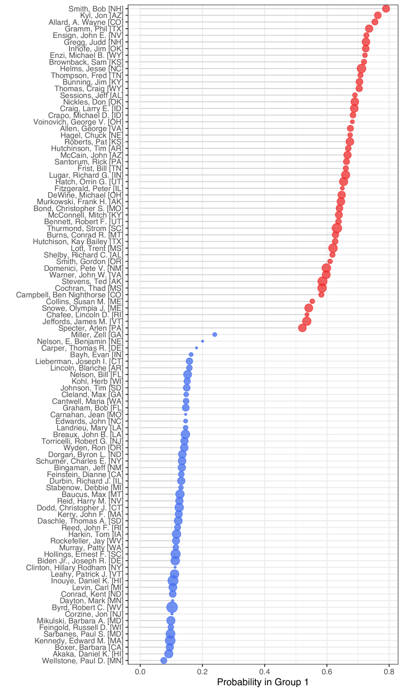
A.8.2 Model estimated coefficients
| Blockmodel estimates | 1 Contentious Bills | 2 Bipartisan Resolutions | 3 Uncontroversial Bills |
| 1 Democrat | 0.2474 | 0.7844 | 1.0000 |
| 2 Republican | 0.1918 | 0.6765 | 0.9999 |
| 3 Junior Power Brokers | 0.2181 | 0.8095 | 1.0000 |
| Coefficient Name | Estimate | SE | ||
| Dyadic predictors | ||||
| No reciprocity history | -6.6168 | 0.1040 | ||
| Log proportional reciprocity | 2.0015 | 0.0146 | ||
| Shared committee | 1.5037 | 0.0504 | ||
| Model Summary Statistics | ||||
| Lower bound | -591.1986 | |||
| Number of dyads | 260667 | |||
| % Obs. in Each Family 1 Block | 0.138 | 0.285 | 0.576 | |
| % Obs. in Each Family 2 Block | 0.578 | 0.360 | 0.062 | |
| Group | Coefficient Name | Estimate | SE | |
| Senator predictors | ||||
| 1 Democrat | Intercept | 4.7867 | 1.3322 | |
| Seniority | 0.5993 | 0.6318 | ||
| Ideology 1 | -5.5500 | 1.2965 | ||
| Ideology 2 | 5.0876 | 1.2912 | ||
| Party-Republican | -3.7291 | 1.3772 | ||
| Sex-Male | 0.4388 | 1.2850 | ||
| 2 Republican | Intercept | 1.5207 | 1.4515 | |
| Seniority | 0.3924 | 0.6318 | ||
| Ideology 1 | 10.3447 | 1.2935 | ||
| Ideology 2 | -2.2911 | 1.2906 | ||
| Party-Republican | 6.1726 | 1.4587 | ||
| Sex-Male | 0.8331 | 1.2850 | ||
| 3 Junior Power Brokers | Intercept | 20.3757 | 1.3299 | |
| Seniority | -0.5417 | 0.6318 | ||
| Ideology 1 | -3.3304 | 1.2916 | ||
| Ideology 2 | -2.2946 | 1.2901 | ||
| Party-Republican | -0.5346 | 1.3436 | ||
| Sex-Male | -0.0602 | 1.2847 | ||
| Bill predictors | ||||
| 1 Contentious Bills | Intercept | 4.2305 | 0.1224 | |
| Topic:Legal | 0.6390 | 0.1033 | ||
| Topic:Social programs Public goods | -0.0517 | 0.0650 | ||
| Topic:Security | 0.8542 | 0.1557 | ||
| Topic:Gov operations | 0.6023 | 0.1179 | ||
| Topic:Other | -1.5853 | 0.0729 | ||
| Sponsor Seniority | -0.0739 | 0.0057 | ||
| Sponsor Ideology 1 | 0.6046 | 0.2433 | ||
| Sponsor Ideology 2 | -0.2777 | 0.1449 | ||
| Sponsor Party-Republican | -0.6889 | 0.1783 | ||
| Sponsor Sex-Male | -0.4856 | 0.0842 | ||
| Group | Coefficient Name | Estimate | SE | |
| Bill predictors (continued) | ||||
| Second Phase | 0.8622 | 0.0789 | ||
| Third Phase | 0.7629 | 0.0553 | ||
| 2 Bipartisan Resolutions | Intercept | 3.3078 | 0.1226 | |
| Topic:Legal | 0.6907 | 0.1036 | ||
| Topic:Social programs Public goods | -0.1533 | 0.0652 | ||
| Topic:Security | 0.9016 | 0.1552 | ||
| Topic:Gov operations | 0.6219 | 0.1178 | ||
| Topic:Other | -1.1869 | 0.0731 | ||
| Sponsor Seniority | -0.0469 | 0.0057 | ||
| Sponsor Ideology 1 | 0.3052 | 0.2438 | ||
| Sponsor Ideology 2 | -0.0983 | 0.1457 | ||
| Sponsor Party-Republican | -0.1289 | 0.1786 | ||
| Sponsor Sex-Male | -0.2849 | 0.0842 | ||
| Second Phase | 0.5371 | 0.0791 | ||
| Third Phase | 0.4116 | 0.0554 | ||
| 3 Uncontroversial Bills | Intercept | 1.6375 | 0.1383 | |
| Topic:Legal | 0.7306 | 0.1210 | ||
| Topic:Social programs Public goods | -0.0564 | 0.0728 | ||
| Topic:Security | 0.8924 | 0.2003 | ||
| Topic:Gov operations | 0.4667 | 0.1461 | ||
| Topic:Other | -0.8497 | 0.0814 | ||
| Sponsor Seniority | -0.0624 | 0.0065 | ||
| Sponsor Ideology 1 | 0.3024 | 0.2697 | ||
| Sponsor Ideology 2 | 0.0398 | 0.1569 | ||
| Sponsor Party-Republican | -0.2731 | 0.1990 | ||
| Sponsor Sex-Male | -0.4408 | 0.0939 | ||
| Second Phase | 0.3514 | 0.0918 | ||
| Third Phase | 0.0778 | 0.0623 | ||
| Estimate | Std. Error | t value | Pr() | |
| Baseline: Group 3 | 6401.593 | 861.9584 | 7.4268 | 0 |
| Group 1 | -3009.3133 | 2112.9178 | -1.4242 | 0.1576 |
| Group 2 | -1447.2995 | 1568.6299 | -0.9227 | 0.3585 |
| Multiple R sq: 0.02296 | Adjusted R sq: 0.00281 | F stat: 1.139 |
On the legislation side of the network, we can explore legislation-level predictor coefficient estimates for each of the three respective latent groups (Table A.8). Perhaps unsurprisingly, sponsor characteristics correlate with mixed membership probabilities across the latent groups, but so too do substantive policy domain types (baseline policy category is “Economy”) and the timing of when the legislation is presented have noticeably large estimated magnitudes of predicted effects, underlining the importance of incorporating bill specific information that delivers contextual and substantive signaling when discussing cosponsorship.
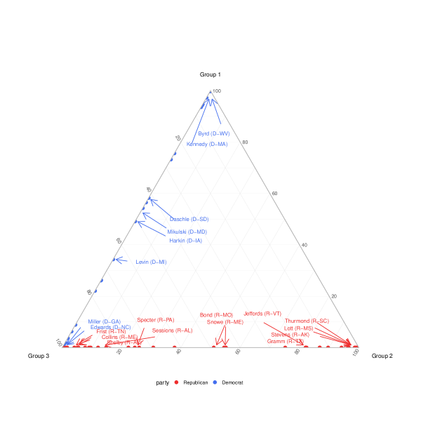
Figure A.6 presents the probabilities of membership for senators across the three latent groups as circles in a ternary plot. For ease of presentation, only a portion of senator names are printed to illustrate examples of legislators with higher membership probabilities in each of the three groups. Senator labels are red for Republicans and blue for Democrats. Table A.5 in the Appendix presents the list of senators with the greatest membership probabilities for each group.