Best-Effort Adaptation

Abstract

We study a problem of best-effort adaptation motivated by several applications and considerations, which consists of determining an accurate predictor for a target domain, for which a moderate amount of labeled samples are available, while leveraging information from another domain for which substantially more labeled samples are at one’s disposal. We present a new and general discrepancy-based theoretical analysis of sample reweighting methods, including bounds holding uniformly over the weights. We show how these bounds can guide the design of learning algorithms that we discuss in detail. We further show that our learning guarantees and algorithms provide improved solutions for standard domain adaptation problems, for which few labeled data or none are available from the target domain. We finally report the results of a series of experiments demonstrating the effectiveness of our best-effort adaptation and domain adaptation algorithms, as well as comparisons with several baselines. We also discuss how our analysis can benefit the design of principled solutions for fine-tuning.

1 Introduction

Consider the following adaptation problem that frequently arises in applications. Suppose we have access to a fair amount of labeled data from a target domain ${\mathscr{P}}$ and to a significantly larger amount of labeled data from a different domain ${\mathscr{Q}}$. How can we best exploit both collections of labeled data to come up with as accurate a predictor as possible for the target domain ${\mathscr{P}}$? We will refer to this problem as the best-effort adaptation problem since we seek the best method to leverage the additional labeled data from ${\mathscr{Q}}$ to come up with a best predictor for ${\mathscr{P}}$. One would imagine that the data from ${\mathscr{Q}}$ should be helpful in improving upon the performance obtained by training only on the ${\mathscr{P}}$ data, if ${\mathscr{Q}}$ is not too different from ${\mathscr{P}}$. The question is how to measure this difference and account for it in the learning algorithm. This best-effort problem differs from standard domain adaptation problems where typically very few or no labeled data from the target is at one’s disposal.

Best-effort adaptation can also be motivated by fairness considerations, such as racial disparities in automated speech recognition (Koenecke et al., 2020). A significant gap has been reported for the accuracy of speech recognition systems when tested on speakers of vernacular English versus non-vernacular English speakers. In practice, there is a substantially larger amount of labeled data available for the non-vernacular domain since it represents a larger population of English speakers. As a result, it might not be possible, with the training data in hand, to achieve an accuracy for vernacular speech similar to the one achieved for non-vernacular speech. Such a recognition system might therefore have only one method for equalizing accuracy between these populations: namely, degrading the system’s performance on the larger population. Alternatively, one could instead formulate the problem of maximizing the performance of the system on the vernacular speakers, leveraging all the data available at hand to find the best-effort predictor for vernacular speakers.

Here, we present a detailed study of best-effort adaptation, including a new and general theoretical analysis of reweighting methods using the notion of discrepancy, as well as new algorithms and empirical evaluations. We further show how our analysis can be extended to that of domain adaptation problems, for which we also design new algorithms and report experimental results.

There is a very broad literature dealing with adaptation solutions for distinct scenarios and we cannot present a comprehensive survey here. Instead, we briefly discuss here the most closely related work and give a detailed discussion of previous work in Appendix A. We also refer the reader to papers such as (Pan and Yang, 2009; Wang and Deng, 2018). Let us add that similar scenarios to best-effort adaptation have been studied in the past under some different names such as inductive transfer or supervised domain adaptation but with the assumption of much smaller labeled data from the target domain (Garcke and Vanck, 2014; Hedegaard et al., 2021).

The work we present includes a significant theoretical component and benefits from prior theoretical analyses of domain adaptation. The theoretical analysis of domain adaptation was initiated by Kifer et al. (2004) and Ben-David et al. (2006) with the introduction of a $d_{A}$-distance between distributions. They used this notion to derive VC-dimension learning bounds for the zero-one loss, which was elaborated on in subsequent works (Blitzer et al., 2008; Ben-David et al., 2010a). Later, Mansour et al. (2009a) and Cortes and Mohri (2011, 2014) presented a general analysis of single-source adaptation for arbitrary loss functions, where they introduced the notion of discrepancy, a divergence measure nicely aligned with domain adaptation. Discrepancy coincides with the $d_{A}$-distance in the special case of the zero-one loss. It takes into account the loss function and hypothesis set and, importantly, can be estimated from finite samples. The authors gave a discrepancy minimization algorithm based on a reweighting of the losses of sample points. We use their notion of discrepancy in our new analysis. Cortes et al. (2019b) presented an extension of the discrepancy minimization algorithm based on the so-called generalized discrepancy, which both incorporates a hypothesis-dependency and works with a less conservative notion of local discrepancy defined by a supremum over a subset of the hypothesis set. The notion of local discrepancy has been since adopted in several recent publications, in the study of active learning or adaptation (de Mathelin et al., 2021; Zhang et al., 2019c, 2020b) and is also used in part of our analysis.

While our main motivation is best-effort adaptation, in Section 3, we present a general analysis that holds for all sample reweighting methods. Our theoretical analysis and learning bounds are new and are based on the notion of discrepancy. They include learning guarantees holding uniformly with respect to the weights, as well as a lower bound suggesting the importance of the discrepancy term in our bounds. Our theory guides the design of principled learning algorithms for best-effort adaptation, best and sbest, that we discuss in detail in Section 4. This includes our estimation of the discrepancy terms via DC-programming (Appendix B.3).

In Section 5, we further show how our analysis can be extended to the case where few labeled data or none are available from the target domain, that is the scenario of (unsupervised or weakly supervised) domain adaptation. Here too, we derive new discrepancy-based learning bounds based on reweighting, including uniform bounds with respect to the weights (Section 5.1). Interestingly, here, an additional set of sample weights naturally appears in the analysis, to account for the absence of labels from the target. Our theoretical analysis leads to the design of a new adaptation algorithms, best-da (Section 5.2). We further discuss in detail how in this scenario labeled discrepancy terms can be upper-bounded in terms of unlabeled ones, including unlabeled local discrepancies, and how some additional amount of labeled data can be beneficial (Section 5.3).

In Section 6, we report the results of experiments with both our best-effort adaptation algorithms and our domain adaptation algorithms demonstrating their effectiveness, as well as comparisons with several baselines. This includes a discussion and empirical analysis of how our results benefit the design of principled solutions for fine-tuning and other few-shot algorithms (Section A.2). We start with the introduction of some preliminary definitions and concepts related to adaptation (Section 2).

2 Preliminaries

We denote by ${\mathscr{X}}$ the input space and ${\mathscr{Y}}$ the output space. In the regression setting, ${\mathscr{Y}}$ is assumed to be a measurable subset of $\mathbb{R}$. We will denote by ${\mathscr{H}}$ a hypothesis set of functions mapping from ${\mathscr{X}}$ to ${\mathscr{Y}}$ and by $\ell\colon{\mathscr{Y}}\times{\mathscr{Y}}\to\mathbb{R}$ a loss function assumed to take values in $[0,1]$.

We will study problems with a source domain ${\mathscr{Q}}$ and target domain ${\mathscr{P}}$, where ${\mathscr{Q}}$ and ${\mathscr{P}}$ are distributions over ${\mathscr{X}}\times{\mathscr{Y}}$. We will denote by $\widehat{\mathscr{Q}}$ the empirical distribution associated to a sample $S$ of size $m$ drawn from ${\mathscr{Q}}^{m}$ and similarly by $\widehat{\mathscr{P}}$ the empirical distribution associated to a sample $S^{\prime}$ of size $n$ drawn from ${\mathscr{P}}^{n}$. We will denote by ${\mathscr{Q}}_{X}$ and ${\mathscr{P}}_{X}$ the marginal distributions of ${\mathscr{Q}}$ and ${\mathscr{P}}$ on ${\mathscr{X}}$. We will denote by $\mathcal{L}({\mathscr{P}},h)$ the population loss of a hypothesis over ${\mathscr{P}}$ defined as: $\mathcal{L}({\mathscr{P}},h)=\operatorname*{\mathbb{E}}_{\begin{subarray}{c}(x,y)\sim{\mathscr{P}}\end{subarray}}\left[\ell((x),y)\right]$.

Several notions of discrepancy have been shown to be adequate measures between distributions for adaptation problems (Kifer et al., 2004; Mansour et al., 2009a; Mohri and Muñoz Medina, 2012; Cortes and Mohri, 2014; Cortes et al., 2019b). We will denote by $\mathrm{dis}({\mathscr{P}},{\mathscr{Q}})$ the labeled discrepancy of ${\mathscr{P}}$ and ${\mathscr{Q}}$, also called ${\mathscr{Y}}$-discrepancy in (Mohri and Muñoz Medina, 2012; Cortes et al., 2019b) and defined by:

$$\mathrm{dis}({\mathscr{P}},{\mathscr{Q}})=\sup_{h\in{\mathscr{H}}}\operatorname*{\mathbb{E}}_{\begin{subarray}{c}(x,y)\sim{\mathscr{P}}\end{subarray}}\left[\ell(h(x),y)\right]-\operatorname*{\mathbb{E}}_{\begin{subarray}{c}(x,y)\sim{\mathscr{Q}}\end{subarray}}\left[\ell(h(x),y)\right].$$ (1)

Note that we are not using absolute values around the difference of expectations, as in the original discrepancy definitions in prior work as the one-sided definition suffices for our analysis. We will denote the version with absolute values as: $\mathrm{Dis}({\mathscr{P}},{\mathscr{Q}})=\max\left\{\mathrm{dis}({\mathscr{P}},{\mathscr{Q}}),\mathrm{dis}({\mathscr{Q}},{\mathscr{P}})\right\}$.

By definition, computing the labeled discrepancy assumes access to labels from both ${\mathscr{P}}$ and ${\mathscr{Q}}$. In contrast, the unlabeled discrepancy, denoted by $\overline{\mathrm{dis}}({\mathscr{P}},{\mathscr{Q}})$, requires no access to such labels

$$\overline{\mathrm{dis}}({\mathscr{P}},{\mathscr{Q}})=\sup_{h,h^{\prime}\in{\mathscr{H}}}\operatorname*{\mathbb{E}}_{\begin{subarray}{c}x\sim{\mathscr{P}}_{X}\end{subarray}}\left[\ell(h(x),h^{\prime}(x))\right]-\operatorname*{\mathbb{E}}_{\begin{subarray}{c}x\sim{\mathscr{Q}}_{X}\end{subarray}}\left[\ell(h(x),h^{\prime}(x))\right].$$ (2)

We will similarly denote by $\overline{\mathrm{Dis}}({\mathscr{P}},{\mathscr{Q}})$ the counterpart of this definition with absolute values. As shown by Mansour et al. (2009a), the unlabeled discrepancy can be accurately estimated from finite (unlabeled) samples from ${\mathscr{Q}}_{X}$ and ${\mathscr{P}}_{X}$ when ${\mathscr{H}}$ admits a favorable Rademacher complexity, for example a finite VC-dimension. The unlabeled discrepancy is a divergence measure tailored to (unsupervised) adaptation that can be upper bounded by the $\ell_{1}$-distance. It coincides with the so-called $d_{A}$-distance introduced by Kifer et al. (2004) in the special case of the zero-one loss. We will also be using the finer notion of local labeled discrepancy for some suitably chosen subsets ${\mathscr{H}}_{1}$ and ${\mathscr{H}}_{2}$ of ${\mathscr{H}}$:

$$\mspace{-40.0mu}\overline{\mathrm{dis}}_{{\mathscr{H}}_{1}\times{\mathscr{H}}_{2}}({\mathscr{P}},{\mathscr{Q}})=\mspace{-10.0mu}\sup_{(h,h^{\prime})\in{\mathscr{H}}_{1}\times{\mathscr{H}}_{2}}\operatorname*{\mathbb{E}}_{\begin{subarray}{c}x\sim{\mathscr{P}}_{X}\end{subarray}}\left[\ell(h(x),h^{\prime}(x))\right]-\operatorname*{\mathbb{E}}_{\begin{subarray}{c}x\sim{\mathscr{Q}}_{X}\end{subarray}}\left[\ell(h(x),h^{\prime}(x))\right].\mspace{-20.0mu}$$ (3)

Local discrepancy (Cortes et al., 2019b) is defined by a supremum over smaller sets and is thus a more favorable quantity. We further extend all the discrepancy definitions just presented to the case where ${\mathscr{P}}$ and ${\mathscr{Q}}$ are finite signed measures over ${\mathscr{X}}\times{\mathscr{Y}}$, using the same expressions as above. We also abusively extend the definition of discrepancy to distributions over sample indices. As an example, given the samples $S$ and $S^{\prime}$ and a distribution ${\mathsf{q}}$ over their $[m+n]$ indices, we define the discrepancy $\mathrm{dis}(\widehat{\mathscr{P}},{\mathsf{q}})$ as follows: $\mathrm{dis}(\widehat{\mathscr{P}},{\mathsf{q}})=\sup_{h\in{\mathscr{H}}}\frac{1}{n}\sum_{i=m+1}^{n}\ell(h(x_{i}),y_{i})-\sum_{i=1}^{m+n}{\mathsf{q}}_{i}\ell(h(x_{i}),y_{i})$.

3 Discrepancy-based generalization bounds

There are many algorithms in adaptation based on various methods for reweighting sample losses and it is natural to seek a similar solution for best-effort adaptation (see Appendix A). We present a general theoretical analysis covering all such sample reweighting methods. We give new discrepancy-based generalization bounds, including learning bounds holding uniformly over the weights.

We assume that the learner has access to a labeled sample $S=\left((x_{1},y_{1}),\ldots,(x_{m},y_{m})\right)$ drawn from ${\mathscr{Q}}^{m}$ and a labeled sample $S^{\prime}=\left((x_{m+1},y_{m+1}),\ldots,(x_{m+n},y_{m+n})\right)$ drawn from ${\mathscr{P}}^{n}$. In the problems we consider, we typically have $m\gg n$, but our analysis applies is general. For a non-negative vector ${\mathsf{q}}$ in $[0,1]^{[m+n]}$, we denote by $\overline{\mathsf{q}}$ the total weight on the first $m$ points: $\overline{\mathsf{q}}=\sum_{i=1}^{m}{\mathsf{q}}_{i}$ and by $\mathfrak{R}_{{\mathsf{q}}}(\ell\circ{\mathscr{H}})$ the ${\mathsf{q}}$-weighted Rademacher complexity:

$$\mathfrak{R}_{{\mathsf{q}}}(\ell\circ{\mathscr{H}})=\operatorname*{\mathbb{E}}_{S,S^{\prime},{\boldsymbol{\sigma}}}\left[\sup_{h\in{\mathscr{H}}}\sum_{i=1}^{m+n}\sigma_{i}{\mathsf{q}}_{i}\ell(h(x_{i}),y_{i})\right],$$ (4)

where the Rademacher variables $\sigma_{i}$ are independent random variables distributed uniformly over $\set{-1,+1}$. The ${\mathsf{q}}$-weighted Rademacher complexity is a natural extension of the Rademacher complexity taking into consideration distinct weights assigned to sample points. It can be upper-bounded as follows in terms of the (unweighted) Rademacher complexity: $\mathfrak{R}_{{\mathsf{q}}}(\ell\circ{\mathscr{H}})\leq\|{\mathsf{q}}\|_{\infty}(m+n)\,\mathfrak{R}_{m+n}(\ell\circ{\mathscr{H}})$, with equality for uniform weights (see Lemma B.5, Appendix B).

The following is a general learning guarantee expressed in terms of the weights ${\mathsf{q}}$. Note that we do not require ${\mathsf{q}}$ to be a distribution over $[m+n]$, that is $\|{\mathsf{q}}\|_{1}$ may not equal one.

Theorem 3.1.

Fix a vector ${\mathsf{q}}$ in $[0,1]^{[m+n]}$. Then, for any $\delta>0$, with probability at least $1-\delta$ over the choice of a sample $S$ of size $m$ from ${\mathscr{Q}}$ and a sample $S^{\prime}$ of size $n$ from ${\mathscr{P}}$, the following holds for all $h\in{\mathscr{H}}$:

$$\mathcal{L}({\mathscr{P}},h)\leq\sum_{i=1}^{m+n}{\mathsf{q}}_{i}\ell(h(x_{i}),y_{i})+\mathrm{dis}\Big{(}\big{[}(1-\|{\mathsf{q}}\|_{1})+\overline{\mathsf{q}}\big{]}{\mathscr{P}},\overline{\mathsf{q}}{\mathscr{Q}}\Big{)}+2\mathfrak{R}_{{\mathsf{q}}}(\ell\circ{\mathscr{H}})+\|{\mathsf{q}}\|_{2}\sqrt{\frac{\log\frac{1}{\delta}}{2}}.$$

This bound is tight as a function of the discrepancy term, as shown by the following theorem, which underscores the importance of that term. The proofs for both theorems are given in Appendix B.

Theorem 3.2.

Fix a distribution ${\mathsf{q}}$ in $\Delta_{m+n}$. Then, for any $\epsilon>0$, there exists $h\in{\mathscr{H}}$ such that, for any $\delta>0$, the following lower bound holds with probability at least $1-\delta$ over the choice of a sample $S$ of size $m$ from ${\mathscr{Q}}$ and a sample $S^{\prime}$ of size $n$ from ${\mathscr{P}}$:

$$\mathcal{L}({\mathscr{P}},h)\geq\sum_{i=1}^{m+n}{\mathsf{q}}_{i}\ell(h(x_{i}),y_{i})+\overline{\mathsf{q}}\mathrm{dis}({\mathscr{P}},{\mathscr{Q}})-2\mathfrak{R}_{{\mathsf{q}}}(\ell\circ{\mathscr{H}})-\|{\mathsf{q}}\|_{2}\sqrt{\frac{\log\frac{1}{\delta}}{2}}-\epsilon.$$

In particular, for $\|{\mathsf{q}}\|_{2},\mathfrak{R}_{{\mathsf{q}}}(\ell\circ{\mathscr{H}})\in O(\frac{1}{\sqrt{m+n}})$, we have:

$$\mathcal{L}({\mathscr{P}},h)\geq\sum_{i=1}^{m+n}{\mathsf{q}}_{i}\ell(h(x_{i}),y_{i})+\overline{\mathsf{q}}\mathrm{dis}({\mathscr{P}},{\mathscr{Q}})+\Omega\left(\frac{1}{\sqrt{m+n}}\right).$$

The bound of Theorem 3.1 cannot be used to choose ${\mathsf{q}}$ since it holds for a fixed choice of that vector. A standard way to derive a uniform bound over ${\mathsf{q}}$ is via covering numbers. That requires applying the union bound to the centers of an $\epsilon$-covering of $[0,1]^{[m+n]}$ for the $\ell_{1}$ distance. But, the corresponding covering number $\mathcal{N}_{1}$ would be in $O(\left(1/\epsilon\right)^{m+n})$, resulting in an uninformative bound, even for $\|{\mathsf{q}}\|_{2}=1/\sqrt{m+n}$, since $\sqrt{\log\mathcal{N}_{1}/m+n}$ would be a constant. Instead, we present an alternative analysis, generalizing Theorem 3.1 to hold uniformly over ${\mathsf{q}}$ in $\left\{{\mathsf{q}}\colon 0<\|{\mathsf{q}}-{\mathsf{p}}^{0}\|_{1}<1\right\}$, where ${\mathsf{p}}^{0}$ could be interpreted as a reference (or ideal) reweighting choice. The proof is presented in Appendix B.

Theorem 3.3.

For any $\delta>0$, with probability at least $1-\delta$ over the choice of a sample $S$ of size $m$ from ${\mathscr{Q}}$ and a sample $S^{\prime}$ of size $n$ from ${\mathscr{P}}$, the following holds for all $h\in{\mathscr{H}}$ and ${\mathsf{q}}\in\left\{{\mathsf{q}}\colon 0\leq\|{\mathsf{q}}-{\mathsf{p}}^{0}\|_{1}<1\right\}$:

$$\mathcal{L}({\mathscr{P}},h)\leq\sum_{i=1}^{m+n}{\mathsf{q}}_{i}\ell(h(x_{i}),y_{i})+\mathrm{dis}\Big{(}\big{[}(1-\|{\mathsf{q}}\|_{1})+\overline{\mathsf{q}}\big{]}{\mathscr{P}},\overline{\mathsf{q}}{\mathscr{Q}}\Big{)}+\mathrm{dis}({\mathsf{q}},{\mathsf{p}}^{0})$$

$$+2\mathfrak{R}_{{\mathsf{q}}}(\ell\circ{\mathscr{H}})+5\|{\mathsf{q}}-{\mathsf{p}}^{0}\|_{1}+\left[\|{\mathsf{q}}\|_{2}+2\|{\mathsf{q}}-{\mathsf{p}}^{0}\|_{1}\right]\left[\sqrt{\log\log_{2}\tfrac{2}{1-\|{\mathsf{q}}-{\mathsf{p}}^{0}\|_{1}}}+\sqrt{\tfrac{\log\frac{2}{\delta}}{2}}\right].$$

Note that for ${\mathsf{q}}={\mathsf{p}}^{0}$, the bound coincides with that of Theorem 3.1.

Learning bounds insights. Theorems 3.1 and 3.3 provide general guarantees for best-effort adaptation. They suggest that for adaptation to succeed via sample reweighting, a favorable balance of several key terms is important. The first term suggests minimizing the ${\mathsf{q}}$-weighted empirical loss. However, the bound advises against doing so at the price of assigning non-zero weights only to a small fraction of the points since that would increase the $\|{\mathsf{q}}\|_{2}$ term. In fact, a comparison with the familiar inverse of square-root of the sample size term appearing in other bounds suggests interpreting $\left(1/\|{\mathsf{q}}\|^{2}_{2}\right)$ as the effective sample size. Note also that when ${\mathsf{q}}$ is a distribution, the second term admits the following simpler form: $\mathrm{dis}\left(\left[(1-\|{\mathsf{q}}\|_{1})+\overline{\mathsf{q}}\right]{\mathscr{P}},\overline{\mathsf{q}}{\mathscr{Q}}\right)=\mathrm{dis}(\overline{\mathsf{q}}{\mathscr{P}},\overline{\mathsf{q}}{\mathscr{Q}})=\overline{\mathsf{q}}\mathrm{dis}({\mathscr{P}},{\mathscr{Q}})$. Thus, the second term of these bounds suggests allocating less weight to the points drawn from ${\mathscr{Q}}$, when the discrepancy $\mathrm{dis}({\mathscr{P}},{\mathscr{Q}})$ is large. The weighted discrepancy term $\mathrm{dis}({\mathsf{q}},{\mathsf{p}}^{0})$ and the $\ell_{1}$-distance $\|{\mathsf{q}}-{\mathsf{p}}_{0}\|_{1}$ in Theorem 3.3 both press ${\mathsf{q}}$ to be chosen relatively closer to the reference ${\mathsf{p}}^{0}$. Finally, the Rademacher complexity term is a familiar measure of the complexity of the hypothesis set, which here additionally takes into consideration the weights.

In Appendix B.2, we compare the bound of Theorem 3.1 with some existing discrepany-based ones and show how they can be recovered as special cases. In particular, we show that the discrepancy-based bound of Cortes et al. (2019b), which is the basis for the discrepancy minimization algorithm of Cortes and Mohri (2014), is always an upper bound on a special case (specific choice of the weights) of the bound of Theorem 3.1.

We note that assigning non-uniform weights to the points in $S$ should not be viewed as unnatural, even though the points are sampled from the same distribution. This is because these weights serve to make the ${\mathsf{q}}$-weighted empirical loss closer to the empirical loss for the target sample. As an example, importance weighting seeks distinct weights for each point based on the source and target distributions. Nevertheless, in Appendix B.2, we consider a simple $\alpha$-reweighting method, which allocates uniform weights to source points. We show that, under some assumptions, even for this very simple choice of the weights, the learning bound can be more favorable than the one for training only on target samples.

Theorem 3.3 suggests choosing $h\in{\mathscr{H}}$ and ${\mathsf{q}}\in\{{\mathsf{q}}\colon 0\leq\|{\mathsf{q}}-{\mathsf{p}}^{0}\|_{1}<1\}$ to minimize the right-hand side of the inequality and seek the best balance between these key terms. This guides the design of our learning algorithms. The following corollary provides a slightly simplified version of Theorem 3.3 (see Appendix B).

Corollary 3.4.

For any $\delta>0$, with probability at least $1-\delta$ over the choice of a sample $S$ of size $m$ from ${\mathscr{Q}}$ and a sample $S^{\prime}$ of size $n$ from ${\mathscr{P}}$, the following holds for all $h\in{\mathscr{H}}$ and ${\mathsf{q}}\in\left\{{\mathsf{q}}\colon 0\leq\|{\mathsf{q}}-{\mathsf{p}}^{0}\|_{1}<1\right\}$:

$$\mathcal{L}({\mathscr{P}},h) \leq\sum_{i=1}^{m+n}{\mathsf{q}}_{i}\ell(h(x_{i}),y_{i})+\overline{\mathsf{q}}\mathrm{dis}({\mathscr{P}},{\mathscr{Q}})+\mathrm{dis}({\mathsf{q}},{\mathsf{p}}^{0})+2\mathfrak{R}_{{\mathsf{q}}}(\ell\circ{\mathscr{H}})$$

$$\quad+6\|{\mathsf{q}}-{\mathsf{p}}^{0}\|_{1}+\left[\|{\mathsf{q}}\|_{2}+2\|{\mathsf{q}}-{\mathsf{p}}^{0}\|_{1}\right]\left[\sqrt{\log\log_{2}\tfrac{2}{1-\|{\mathsf{q}}-{\mathsf{p}}^{0}\|_{1}}}+\sqrt{\frac{\log\tfrac{2}{\delta}}{2}}\right].$$

4 Best-Effort adaptation algorithms

In this section, we describe new learning algorithms for best-effort adaptation directly benefiting from the theoretical analysis of the previous section.

Optimization problem, best and sbest algorithms. The previous section suggests seeking $h\in{\mathscr{H}}$ and ${\mathsf{q}}\in[0,1]^{m+n}$ to minimize the bound of Theorem 3.3 or that of Corollary 3.4. To simplify the discussion, we will focus on the algorithm derived from Corollary 3.4. A similar but finer algorithm consists instead of using directly Theorem 3.3.

Assume that ${\mathscr{H}}$ is a subset of a normed vector space and that the Rademacher complexity term can be bounded by an upper bound on the norm squared $\|h\|^{2}$. Then, using the shorthand $d_{i}=\mathrm{dis}({\mathscr{P}},{\mathscr{Q}})1_{i\in[m]}$, the optimization problem can be written as:

$$\min_{h\in{\mathscr{H}},{\mathsf{q}}\in[0,1]^{m+n}} \sum_{i=1}^{m+n}{\mathsf{q}}_{i}\left[\ell(h(x_{i}),y_{i})+d_{i}\right]+\mathrm{dis}({\mathsf{q}},{\mathsf{p}}^{0})+\lambda_{\infty}\|{\mathsf{q}}\|_{\infty}\|h\|^{2}$$

$$+\lambda_{1}\|{\mathsf{q}}-{\mathsf{p}}^{0}\|_{1}+\lambda_{2}\|{\mathsf{q}}\|^{2}_{2},$$

where $\lambda_{1}$, $\lambda_{2}$ and $\lambda_{\infty}$ are non-negative hyperparameters. A natural choice for ${\mathsf{p}}^{0}$ in our scenario is the uniform distribution over $S^{\prime}$, which is the empirical distribution in the absence of any point from a different distribution ${\mathscr{Q}}$. We will refer by best to an algorithm seeking to minimize this objective. We will also consider a simpler version of our algorithm, sbest, where we upper-bound $\mathrm{dis}({\mathsf{q}},{\mathsf{p}}^{0})$ by $\|{\mathsf{q}}-{\mathsf{p}}^{0}\|_{1}$, in which case this additional term is subsumed by the existing one with $\lambda_{1}$ factor.

When the loss function $\ell$ is convex with respect to its first argument, the objective function is convex in $h$ and in ${\mathsf{q}}$. In particular, $\mathrm{dis}({\mathsf{q}},{\mathsf{p}}^{0})$ is a convex function of ${\mathsf{q}}$ as a supremum of convex functions (affine functions in ${\mathsf{q}}$): $\mathrm{dis}({\mathsf{q}},{\mathsf{p}}^{0})=\sup_{h\in{\mathscr{H}}}\left\{\sum_{i=1}^{m+n}({\mathsf{q}}_{i}-{\mathsf{p}}^{0}_{i})\ell(h(x_{i}),y_{i})\right\}$. But, the objective function is not jointly convex.

Alternating minimization solution. One method for solving the problem consists of alternating minimization (or block coordinate descent), that is of minimizing the objective over ${\mathscr{H}}$ for a fixed value of ${\mathsf{q}}$ and next of minimizing with respect to ${\mathsf{q}}$ for a fixed value of $h$. In general, this method does not benefit from convergence guarantees, although there is a growing body of literature proving guarantees under various assumptions (Grippo and Sciandrone, 2000; Li et al., 2019; Beck, 2015).

DC-programming solution. An alternative solution consists of casting the problem as an instance of DC-programming (difference of convex) by rewriting the objective as a difference. Note that for any non-negative and convex function $f$ and any non-decreasing and convex function $\Psi$ defined over $\mathbb{R}_{+}$, $\Psi\circ f$ is convex: for all $(x,x^{\prime})\in{\mathscr{X}}^{2}$ and $\alpha\in[0,1]$,

$$(\Psi\circ f)(\alpha x+(1-\alpha)x^{\prime}) \leq\Psi(\alpha f(x)+(1-\alpha)f(x^{\prime}))$$

$$\leq\alpha(\Psi\circ f)(x)+(1-\alpha)(\Psi\circ f)(x^{\prime}),$$

where the first inequality holds by the convexity of $f$ and the non-decreasing property of $\Psi$ and the last one by the convexity of $\Psi$. In particular, for any non-negative and convex function $f$, $f^{2}$ is convex. Thus, we can rewrite the non-jointly convex terms of the objective as the following DC-decompositions:

$${\mathsf{q}}_{i}\ell(h(x_{i}),y_{i}) =\frac{1}{2}\left[\left[{\mathsf{q}}_{i}+u\right]^{2}-\left[{\mathsf{q}}_{i}^{2}+u^{2}\right]\right],$$

$$\|{\mathsf{q}}\|_{\infty}\|h\|^{2} =\frac{1}{2}\left[\left[\|{\mathsf{q}}\|_{\infty}+\|h\|^{2}\right]^{2}-\left[\|{\mathsf{q}}\|^{2}_{\infty}+\|h\|^{2}\right]\right],$$

where $u=\ell(h(x_{i}),y_{i})$. We can then use the DCA algorithm of Tao and An (1998), (see also Tao and An (1997)), which in our differentiable case coincides with the CCCP algorithm of Yuille and Rangarajan (2003), further analyzed by Sriperumbudur et al. (2007). The DCA algorithm guarantees convergence to a critical point. The global optimum can be found by combining DCA with a branch-and-bound or cutting plane method (Tuy, 1964; Horst and Thoai, 1999; Tao and An, 1997).

Discrepancy estimation. Our algorithm requires estimating the discrepancy terms. We discuss our DC-programming solution to this problem in detail in Appendix B.3.

As already pointed, our learning bounds are general and can be used for the analysis of various specific reweighting methods with bounded weights, including discrepancy minimization (Cortes and Mohri, 2014), KMM (Huang et al., 2006), KLIEP (Sugiyama et al., 2007b), importance weighting (Cortes et al., 2010), when the weights are bounded, and many others. However, unlike our algorithms, which simultaneously learn the weights and the hypothesis and directly benefit from the learning bounds of the previous section, these algorithms typically consist of two stages and do not exploit the guarantees discussed: in the first stage, they determine some weights ${\mathsf{q}}$, irrespective of the labeled samples and the empirical loss; in the second stage, they use these weights to learn a hypothesis minimizing the ${\mathsf{q}}$-weighted empirical loss. Additionally, some methods admit other specific drawbacks. For example, it was shown by Cortes et al. (2010), both theoretically and empirically, that, in general, importance weighting may not succeed. Note also that the method relies only on the ratio of the densities and does not take into account, unlike the discrepancy, the hypothesis set and the loss function.

5 Domain adaptation

The analysis of Section 3 can also be used to derive general discrepancy-based guarantees for domain adaptation, where the learner has access to few or no labeled points from the target domain. In this section, we analyze the case where the input points in $S^{\prime}$ are unlabeled. Our analysis can be straightforwardly extended to the case where a small fraction of the labels in $S^{\prime}$ are available. Our theoretical analysis leads to the design of new algorithms for domain adaptation.

5.1 Domain adaptation generalization bounds

For convenience, in this section, we will use a different notation for the weights on $S$ and $S^{\prime}$: ${\mathsf{q}}\in[0,1]^{m}$ for the weights on $S$, ${\mathsf{q}}^{\prime}\in[0,1]^{n}$ for the weights on $S^{\prime}$. The labels of the points in $S^{\prime}$ appear in the first term of the bound of Theorem 3.1, the ${\mathsf{q}}$-weighted empirical loss. Since they are not available, we upper-bound the empirical loss in terms of a ${\mathsf{p}}$-weighted empirical loss and a discrepancy term:

$$\sum_{i=1}^{m}{\mathsf{q}}_{i}\ell(h(x_{i}),y_{i})+\sum_{i=1}^{n}{\mathsf{q}}^{\prime}_{i}\ell(h(x_{m+i}),y_{m+i})\leq\sum_{i=1}^{m}({\mathsf{q}}_{i}+{\mathsf{p}}_{i})\ell(h(x_{i}),y_{i})+\mathrm{dis}({\mathsf{q}}^{\prime},{\mathsf{p}}),$$ (5)

for any weight vector ${\mathsf{p}}\in[0,1]^{m}$. This yields immediately the following theorem.

Theorem 5.1.

Fix the vectors ${\mathsf{q}}$ in $[0,1]^{[m]}$ and ${\mathsf{q}}^{\prime}\in[0,1]^{n}$. Then, for any $\delta>0$, with probability at least $1-\delta$ over the choice of a sample $S$ of size $m$ from ${\mathscr{Q}}$ and a sample $S^{\prime}$ of size $n$ from ${\mathscr{P}}$, the following holds for all ${\mathsf{p}}$ in $[0,1]^{[m]}$ and $h\in{\mathscr{H}}$:

$$\mathcal{L}({\mathscr{P}},h) \leq\sum_{i=1}^{m}({\mathsf{q}}_{i}+{\mathsf{p}}_{i})\ell(h(x_{i}),y_{i})+\mathrm{dis}({\mathsf{q}}^{\prime},{\mathsf{p}})+\mathrm{dis}\Big{(}\big{[}1-\|{\mathsf{q}}^{\prime}\|_{1}\big{]}{\mathscr{P}},\|{\mathsf{q}}\|_{1}{\mathscr{Q}}\Big{)}$$

$$\quad+2\mathfrak{R}_{({\mathsf{q}},{\mathsf{q}}^{\prime})}(\ell\circ{\mathscr{H}})+\sqrt{\frac{\left(\|{\mathsf{q}}\|^{2}_{2}+\|{\mathsf{q}}^{\prime}\|^{2}_{2}\right)\log\frac{1}{\delta}}{2}}.$$

This learning bound can be extended to hold uniformly over

$$\left\{({\mathsf{q}},{\mathsf{q}}^{\prime})\in[0,1]^{m}\times[0,1]^{n}\colon 0<\|({\mathsf{q}},{\mathsf{q}}^{\prime})-{\mathsf{p}}^{0}\|_{1}<1\right\}$$

and all ${\mathsf{p}}$ in $[0,1]^{[m]}$, where ${\mathsf{p}}^{0}$ is a reference (or ideal) reweighting choice over the $(m+n)$ points (see Theorem C.1 and Corollary C.3 in Appendix C). Note that, here, both ${\mathsf{p}}$ and ${\mathsf{q}}^{\prime}$ can be chosen to make the weighted-discrepancy term $\mathrm{dis}({\mathsf{q}}^{\prime},{\mathsf{p}})$ smaller. Several of the comments on Theorem 3.1 similarly apply here. In particular, it is worth pointing out that the learning bound of Cortes et al. (2019b) can be recovered for a specific choice of the weights. This holds even in the special case where ${\mathsf{q}}=0$ and where ${\mathsf{q}}^{\prime}$ is a distribution:

$$\mathcal{L}({\mathscr{P}},h)\leq\sum_{i=1}^{m}{\mathsf{p}}_{i}\ell(h(x_{i}),y_{i})+\mathrm{dis}({\mathsf{q}}^{\prime},{\mathsf{p}})+2\mathfrak{R}_{{\mathsf{q}}^{\prime}}(\ell\circ{\mathscr{H}})+\|{\mathsf{q}}^{\prime}\|_{2}\sqrt{\frac{\log\frac{1}{\delta}}{2}}.$$

In that case, choosing ${\mathsf{q}}^{\prime}$ to be the empirical distribution on $S^{\prime}$ leads to the bound of Cortes et al. (2019b) (see also inequality (17), in Appendix B.2). An alternative choice of the weights may lead to a smaller discrepancy term $\mathrm{dis}({\mathsf{q}}^{\prime},{\mathsf{p}})$ and a better guarantee overall. Our learning algorithm will seek an optimal choice for the weights.

The discrepancy quantities appearing in the bound of the theorem cannot be estimated in the absence of labels for $S^{\prime}$. Thus, we need to resort to upper-bounds expressed in terms of unlabeled discrepancies, using only unlabeled data from ${\mathscr{P}}$. A detailed analysis is presented in Appendix 5.3.

5.2 Domain adaptation best-da algorithm

The analysis of the previous section suggests seeking $h\in{\mathscr{H}}$, ${\mathsf{q}}$ and ${\mathsf{p}}$ in $[0,1]^{m}$ and ${\mathsf{q}}^{\prime}$ in $[0,1]^{n}$ to minimize the bound of Theorem C.1 or that of Corollary C.3. As in Section 4, assume that ${\mathscr{H}}$ is a subset of a normed vector space and that the Rademacher complexity term can be bounded in terms of an upper bound on the norm squared $\|h\|^{2}$. Then, the optimization problem corresponding to Corollary C.3 can be written as follows:

$$\min_{\begin{subarray}{c}h\in{\mathscr{H}},{\mathsf{q}},{\mathsf{p}}\in[0,1]^{m}\\ {\mathsf{q}}^{\prime}\in[0,1]^{n}\end{subarray}} \sum_{i=1}^{m}({\mathsf{q}}_{i}+{\mathsf{p}}_{i})\,\ell(h(x_{i}),y_{i})+\|{\mathsf{q}}\|_{1}\overline{d}+\overline{\mathrm{dis}}({\mathsf{q}}^{\prime},{\mathsf{p}})+\overline{\mathrm{dis}}(({\mathsf{q}},{\mathsf{q}}^{\prime}),{\mathsf{p}}^{0})$$ (6)

$$+\lambda_{\infty}\|({\mathsf{q}},{\mathsf{q}}^{\prime})\|_{\infty}\,\|h\|^{2}+\lambda_{1}\|({\mathsf{q}},{\mathsf{q}}^{\prime})-{\mathsf{p}}^{0}\|_{1}+\lambda_{2}(\|{\mathsf{q}}\|^{2}_{2}+\|{\mathsf{q}}^{\prime}\|^{2}_{2}),$$

where $\lambda_{1}$, $\lambda_{2}$ and $\lambda_{\infty}$ are non-negative hyperparameters and where we used the shorthand $\overline{d}=\overline{\mathrm{dis}}({\mathscr{P}},{\mathscr{Q}})$. We are omitting subscripts to simplify the presentation but, as discussed in the previous section, the unlabeled discrepancies in the optimization problem may be local unlabeled discrepancies, which are finer quantities. As in the best-effort adaptation, a natural choice for ${\mathsf{p}}^{0}$ in the domain adaptation scenario is the uniform distribution over the input points of $S^{\prime}$. In practice, specific applications may motivate better choices.

We will refer by best-da to the algorithm seeking to minimize this objective. Our comments and analysis of the best optimization (Section 4) apply similarly here. In particular, the problem can be similarly cast as a DC-programming problem or a convex optimization problem. The unlabeled discrepancy term $\overline{d}=\overline{\mathrm{dis}}({\mathscr{P}},{\mathscr{Q}})$ can be accurately estimated from $\overline{\mathrm{dis}}({\mathscr{P}},{\mathscr{Q}})$. In Appendix C.4, we show in detail how to compute $\overline{\mathrm{dis}}({\mathscr{P}},{\mathscr{Q}})$ and how to evaluate the sub-gradients of the weighted discrepancy terms.

Discussion of new best-da algorithm

Our best-da algorithm benefits from more favorable guarantees than previous discrepancy-based algorithms (Mansour et al., 2009a; Cortes and Mohri, 2014; Cortes et al., 2019b) and algorithms seeking to minimize the learning bound (17), with the unlabeled discrepancy upper bounded by the label discrepancy. This is because, as already pointed out, best-da is based on a learning guarantee that admits as a special case (17). Thus, the best choice of the weights and predictor sought by the algorithm include those corresponding to previous algorithms as a special case.

Moreover, as discussed in Section 3, our upper bounds in terms of local discrepancy are finer than those used in previous work. In particular, best-da improves upon the dm algorithm (discrepancy minimization) of Cortes and Mohri (2014), which has been shown empirically by the authors to outperform other domain adaptation baselines in regression tasks. dm seeks to minimize (17) via a two-stage method, by first seeking weights that minimize the unlabeled weighted-discrepancy (second term) and subsequently seeking $h\in{\mathscr{H}}$ to minimize the empirical loss for that fixed choice of ${\mathsf{q}}$. This two-stage method may be suboptimal, compared to an algorithm seeking to directly minimize the bound to find $(h,{\mathsf{q}})$. The solution ${\mathsf{q}}$ found to minimize the discrepancy term in the first stage may, for example, assign significantly larger weights to some sample points, which could lead to a poor choice of the predictor in the second stage.

An alternative sophisticated technique based on the so-called generalized discrepancy is advocated by Cortes et al. (2019b). The main benefit of this technique is to allow for the weights to be chosen as a function of the hypotheses, unlike the two-stage dm solution of Cortes and Mohri (2014). Our best-da algorithm, however, already offers that advantage since the hypothesis $h$ and the weights ${\mathsf{q}}$, ${\mathsf{q}}^{\prime}$ and ${\mathsf{p}}$ are sought simultaneously as a solution of the optimization problem. Note, however that the choice of the weights in the generalized discrepancy method does not take into consideration the empirical losses, unlike our algorithm. Furthermore, best-da minimizes a learning bound admitting as a special case (17), the best learning guarantee presented by the authors in support of their algorithm. Let us add that authors state that their guarantee for the generalized discrepancy method is not comparable to that of dm algorithm.

5.3 Labeled discrepancy upper bounds

The analysis of Section 3 is based on the labeled discrepancy measure $\mathrm{dis}({\mathscr{P}},{\mathscr{Q}})$ or its estimate from finite samples $\mathrm{dis}(\widehat{\mathscr{P}},\widehat{\mathscr{Q}})$, which assumes access to labeled data from the target distribution ${\mathscr{P}}$. In typical domain adaptation problems, however, there is little labeled data or none from the target domain ${\mathscr{P}}$. Thus, instead we need to resort to an upper-bound on $\mathrm{dis}({\mathscr{P}},{\mathscr{Q}})$ in terms of the unlabeled discrepancy, which only uses unlabeled data from ${\mathscr{P}}$.

We will discuss two types of upper bounds, first in the special case of the squared loss, next in the case of an arbitrary $\mu$-Lipschitz loss. Our analysis benefits from that of previous work (Cortes and Mohri, 2014; Cortes et al., 2019b) but improves upon that, as discussed later.

Squared loss. Here, we give an upper bound on the labeled discrepancy in the case of the squared loss. For any hypothesis $h_{0}\in{\mathscr{H}}$, we denote by $\delta_{{\mathscr{H}},h_{0}}(\widehat{\mathscr{P}},\widehat{\mathscr{Q}})$ the squared-loss label discrepancy of $\widehat{\mathscr{P}}$ and $\widehat{\mathscr{Q}}$:

$$\delta_{{\mathscr{H}},h_{0}}(\widehat{\mathscr{P}},\widehat{\mathscr{Q}})=\sup_{h\in{\mathscr{H}}}\,\lvert\operatorname*{\mathbb{E}}_{\begin{subarray}{c}(x,y)\sim\widehat{\mathscr{P}}\end{subarray}}\left[h(x)\left(y-h_{0}(x)\right)\right]-\operatorname*{\mathbb{E}}_{\begin{subarray}{c}(x,y)\sim\widehat{\mathscr{Q}}\end{subarray}}\left[h(x)\left(y-h_{0}(x)\right)\right]\rvert.$$ (7)

Lemma 5.2.

Let $\ell$ be the squared loss. Then, for any hypothesis $h_{0}$ in ${\mathscr{H}}$, the following upper bound holds for the labeled discrepancy:

$$\mathrm{dis}(\widehat{\mathscr{P}},\widehat{\mathscr{Q}})\leq\overline{\mathrm{dis}}_{{\mathscr{H}}\times\set{h_{0}}}(\widehat{\mathscr{P}},\widehat{\mathscr{Q}})+2\delta_{{\mathscr{H}},h_{0}}(\widehat{\mathscr{P}},\widehat{\mathscr{Q}}).$$

The proof is given below in Appendix C.2. The local unlabeled discrepancy $\overline{\mathrm{dis}}_{{\mathscr{H}}\times\set{h_{0}}}(\widehat{\mathscr{P}},\widehat{\mathscr{Q}})$ captures the closeness of the input distributions $\widehat{\mathscr{P}}_{X}$ and $\widehat{\mathscr{Q}}_{X}$. It is a significantly more favorable term that the standard unlabeled discrepancy since it admits only a maximum over $h\in{\mathscr{H}}$ and not over both $h$ and $h^{\prime}$ in ${\mathscr{H}}$.

For a suitable choice of $h_{0}\in{\mathscr{H}}$, the term $\delta_{{\mathscr{H}},h_{0}}(\widehat{\mathscr{P}},\widehat{\mathscr{Q}})$ captures the closeness of the empirical output labels on $\widehat{\mathscr{P}}$ and $\widehat{\mathscr{Q}}$. Note that for $\widehat{\mathscr{P}}=\widehat{\mathscr{Q}}$, we have $\delta_{{\mathscr{H}},h_{0}}(\widehat{\mathscr{P}},\widehat{\mathscr{Q}})=0$ for any $h_{0}\in{\mathscr{H}}$. When the covariate-shift assumption holds and the problem is separable, $h_{0}$ can be chosen so that $\delta_{{\mathscr{H}},h_{0}}(\widehat{\mathscr{P}},\widehat{\mathscr{Q}})=0$. More generally, when $h_{0}$ can be chosen so that $|y-h_{0}(x)|$ is relatively small on both samples corresponding to $\widehat{\mathscr{P}}$ and $\widehat{\mathscr{Q}}$ and the hypotheses $h\in{\mathscr{H}}$ are bounded by some $M>0$, then $\delta_{{\mathscr{H}},h_{0}}(\widehat{\mathscr{P}},\widehat{\mathscr{Q}})$ is relatively small. Note that adaptation is in general not possible if the learner receives vastly different labels on the source domain ${\mathscr{Q}}$ than those corresponding to the target ${\mathscr{P}}$.

$\mu$-Lipschitz loss. Here, we give an upper bound on the labeled discrepancy for any $\mu$-Lipschitz loss. For any hypothesis $h_{0}\in{\mathscr{H}}$, we denote by $\eta_{{\mathscr{H}},h_{0}}(\widehat{\mathscr{P}},\widehat{\mathscr{Q}})$ the Lipschitz loss labeled discrepancy defined by

$$\eta_{{\mathscr{H}},h_{0}}(\widehat{\mathscr{P}},\widehat{\mathscr{Q}})=\operatorname*{\mathbb{E}}_{(x,y)\sim\widehat{\mathscr{P}}}\left[\left\lvert y-h_{o}(x)\right\rvert\right]+\operatorname*{\mathbb{E}}_{(x,y)\sim\widehat{\mathscr{Q}}}\left[\left\lvert y-h_{o}(x)\right\rvert\right].$$ (8)

Lemma 5.3.

Let $\ell$ be a loss function that is $\mu$-Lipschitz with respect to its second argument. Then, for any hypothesis $h_{0}$ in ${\mathscr{H}}$, the following upper bound holds for the labeled discrepancy:

$$\mathrm{dis}(\widehat{\mathscr{P}},\widehat{\mathscr{Q}})\leq\overline{\mathrm{dis}}_{{\mathscr{H}}\times\set{h_{0}}}(\widehat{\mathscr{P}},\widehat{\mathscr{Q}})+\mu\,\eta_{{\mathscr{H}},h_{0}}(\widehat{\mathscr{P}},\widehat{\mathscr{Q}}).$$

The proof is given below in Appendix C.3.

The Lipschitz loss labeled discrepancy $\eta_{{\mathscr{H}},h_{0}}(\widehat{\mathscr{P}},\widehat{\mathscr{Q}})$ is a coarser quantity than $\delta_{{\mathscr{H}},h_{0}}(\widehat{\mathscr{P}},\widehat{\mathscr{Q}})$. In particular, even when $\widehat{\mathscr{P}}=\widehat{\mathscr{Q}}$, $\eta_{{\mathscr{H}},h_{0}}(\widehat{\mathscr{P}},\widehat{\mathscr{Q}})$ is not zero. However, as with $\delta_{{\mathscr{H}},h_{0}}(\widehat{\mathscr{P}},\widehat{\mathscr{Q}})$ it captures the closeness of the output labels on $\widehat{\mathscr{P}}$ and $\widehat{\mathscr{Q}}$. When $h_{0}$ can be chosen so that the sum of expected values $|y-h_{0}(x)|$ is relatively small on both samples corresponding to $\widehat{\mathscr{P}}$ and $\widehat{\mathscr{Q}}$ then, $\eta_{{\mathscr{H}},h_{0}}(\widehat{\mathscr{P}},\widehat{\mathscr{Q}})$ is relatively small. As already pointed out, adaptation is not possible when the learner received very different labels on the two domains.

The upper bounds of Lemmas 5.2 and 5.3 hold in the stochastic setting and are thus more general than those derived for the deterministic label setting in previous work (Cortes and Mohri, 2014; Cortes et al., 2019b). They are also finer bounds expressed in terms of the more favorable local discrepancy and somewhat more favorable label discrepancy terms defined in terms of expectation over the empirical distributions as opposed to a supremum.

In both the squared loss and Lipschitz cases, when a relatively small labeled sample $S^{\prime}$ drawn i.i.d. from ${\mathscr{P}}$ is available, we can use it to select $h_{0}$ via

$$h_{0}=\operatorname*{argmin}_{h_{0}\in{\mathscr{H}}}\delta_{{\mathscr{H}},h_{0}}(\widehat{\mathscr{P}}_{S^{\prime}},\widehat{\mathscr{Q}})\text{ or }h_{0}=\operatorname*{argmin}_{h_{0}\in{\mathscr{H}}}\eta_{{\mathscr{H}},h_{0}}(\widehat{\mathscr{P}}_{S^{\prime}},\widehat{\mathscr{Q}}).$$

When no labeled data from the target domain is at our disposal, we cannot choose $h_{0}$ by leveraging any existing information. We can then assume that $\min_{h_{0}\in{\mathscr{H}}}\delta_{{\mathscr{H}},h_{0}}(\widehat{\mathscr{P}},\widehat{\mathscr{Q}})\ll 1$ in the squared loss case or $\min_{h_{0}\in{\mathscr{H}}}\eta_{{\mathscr{H}},h_{0}}(\widehat{\mathscr{P}},\widehat{\mathscr{Q}})\ll 1$ in the Lipschitz case, that is that the source labels are relatively close to the target ones based on these measures and use the standard unlabeled discrepancy:

$$\mathrm{dis}(\widehat{\mathscr{P}},\widehat{\mathscr{Q}}) \leq\overline{\mathrm{dis}}(\widehat{\mathscr{P}},\widehat{\mathscr{Q}})+2\min_{h_{0}\in{\mathscr{H}}}\delta_{{\mathscr{H}},h_{0}}(\widehat{\mathscr{P}},\widehat{\mathscr{Q}})$$

$$\mathrm{dis}(\widehat{\mathscr{P}},\widehat{\mathscr{Q}}) \leq\overline{\mathrm{dis}}(\widehat{\mathscr{P}},\widehat{\mathscr{Q}})+\mu\min_{h_{0}\in{\mathscr{H}}}\eta_{{\mathscr{H}},h_{0}}(\widehat{\mathscr{P}},\widehat{\mathscr{Q}}).$$

6 Experimental evaluation

We evaluated our algorithms in best-effort adaptation, fine-tuning, and (unsupervised) domain adaptation. We performed cross-validation using labeled data from the target to pick the hyperparameters for our algorithms and the baselines. See Appendix D for details on data and experimental procedures. For all the experiments we use the sbest algorithm.

6.1 Best-Effort adaptation

Here we have labeled data both from the source and the target. Two natural baselines are to train solely on ${\mathscr{P}}$, or solely ${\mathscr{Q}}$. A third baseline is the $\alpha$-reweighted ${\mathsf{q}}$ as described in Appendix B.2.

Figure 1: Simulated data.

Simulated data. The goal of this experiment was to demonstrate that sbest outperforms the simple baselines just mentioned and to compare the performance of the Alternate Minimization (sbest-AM) and the DC-programming (sbest-DC) optimization solutions.

We consider a linear binary classification task with the labels for ${\mathscr{P}}$ generated as $\text{sgn}(w_{p}\cdot x)$ for a randomly chosen unit vector $w_{p}$. The distribution ${\mathscr{Q}}$ admits two parts. For $\eta\in(0.5,1)$, $(1-\eta)m$ examples are labeled according to $\text{sgn}(w_{q}\cdot x)$ where $\|w_{p}-w_{q}\|\leq\epsilon$, while the remaining examples are set to a fixed vector $u$ and labeled $+1$. These $\eta m$ examples represent the noise in ${\mathscr{Q}}$ and, as $\eta$ increases, $\mathrm{dis}({\mathscr{P}},{\mathscr{Q}})$ gets larger. For this setting, we evaluated the baselines and sbest with the logistic loss and linear hypotheses. See Appendix D for more details and examples.

Figure 1 shows the performance for $\eta=10\%$ as $n$ increases. For small sizes, $n$, of the target data ${\mathscr{P}}$, both $\alpha$-reweighting and the baseline that trains solely on ${\mathscr{Q}}$ are significantly impacted. This is because these methods cannot distinguish between non-noisy and noisy data points. On the other hand, both sbest-AM and sbest-DC can counter the effect of the noise by generating ${\mathsf{q}}$-weights that are predominantly supported on the non-noisy samples. The performance of these algorithms is fairly independent of the size of $n$ as, for $\eta=10\%$, they can still make an effective use of 90% of the $m=1000$ examples. As $n$ increases, $\alpha$-reweighting and the baseline that trains solely on ${\mathscr{P}}$ reach the performance of sbest. We also note that sbest-AM and sbest-DC perform equivalently and in all the following experiments, we use sbest-AM. For experiments with other values of $\eta$ and further discussion of this experiment, see Appendix D.

6.2 Fine-tuning tasks

Table 1: Performance of sbest, compared to baseline approaches in CIFAR-10.

Fine-tuning	Train on ${\mathscr{P}}$	gapBoost	sbest
Last layer (CIFAR-10)	$88.61\pm.43$	$87.1\pm.01$	$\mathbf{89.62\pm.32}$
Full model (CIFAR-10)	$90.18\pm.31$	$90.8\pm.02$	$\mathbf{92.30\pm.24}$
Last layer (Civil)	$63.1\pm.12$	$64.7\pm.11$	$\mathbf{65.8\pm.12}$
Full model (Civil)	$65.8\pm.01$	$67.2\pm.01$	$\mathbf{68.3\pm.14}$

Here, we applied our algorithms to fine-tuning pre-trained models in classification. In the pre-training/fine-tuning paradigm (Raffel et al., 2019), a model is pre-trained on a generalist dataset (coming from ${\mathscr{Q}}$). The model is then fine-tuned on a task-specific dataset (generated from ${\mathscr{P}}$). Two predominantly used fine-tuning approaches are last-layer fine-tuning (Subramanian et al., 2018; Kiros et al., 2015) and full-model fine-tuning (Howard and Ruder, 2018). In the former, the representations obtained from the last layer of the pre-trained model are used to train a simple model (often a linear hypothesis) on the data from ${\mathscr{P}}$. We chose the simple model to be a multi-class logistic regression model. In the latter approach, the model is initialized from the pre-trained model and all the parameters are fine-tuned (often via gradient descent) on ${\mathscr{P}}$. We explored the additional advantages of combining data from both ${\mathscr{P}}$ and ${\mathscr{Q}}$ during fine-tuning. There has been recent interest in carefully combining various tasks/data for the purpose of fine-tuning and avoid the phenomenon of “negative transfer” (Aribandi et al., 2021). Our proposed theory presents a principled approach.

We used the CIFAR-10 vision dataset (Krizhevsky et al., 2009) and formed a pre-training task (source) by combining data from classes: {’airplane’, ’automobile’, ’bird’, ’cat’, ’deer’, ’dog’}. For this task we use a standard ResNet-18 architecture (He et al., 2016). The fine-tuning task (target) consists of data from classes: {’frog’, ’horse’, ’ship’, ’truck’}. In addition, we also used the Civil Comments dataset. For this we used a BERT-small model (Devlin et al., 2018) for pre-training. For more detail on the dataset and experimental procedure, see Appendix D. As can be seen from Table 1, sbest comfortably outperforms both the standard approach of training just on ${\mathscr{P}}$, as well as gapBoost.

7 Conclusion

We presented a comprehensive study of best-effort adaptation (or supervised adaptation), including a new discrepancy-based theoretical analysis, algorithms benefiting from the corresponding learning guarantees, as well as a series of empirical results demonstrating the performance of these algorithms in several tasks. We further showed how our analysis can be leveraged to derive learning guarantees in domain adaptation, as well as new enhanced adaptation algorithms. Our analysis and algorithms are likely to be useful in the study of other adaptation scenarios and admit a variety of other applications. In fact, our analysis applies to any sample reweighting method.

Appendix A Related work

A.1 Adaptation and transfer learning

Discrepancy-based adaptation theory. The work we present includes a significant theoretical component and benefits from prior theoretical analyses of domain adaptation. The theoretical analysis of domain adaptation was initiated by Kifer et al. (2004) and Ben-David et al. (2006) with the introduction of a $d_{A}$-distance between distributions. They used this notion to derive VC-dimension learning bounds for the zero-one loss, which was elaborated on in follow-up publications like (Blitzer et al., 2008; Ben-David et al., 2010a). Later, Mansour et al. (2009a) and Cortes and Mohri (2011, 2014) presented a general analysis of single-source adaptation for arbitrary loss functions, where they introduced the notion of discrepancy, which they argued is a divergence measure tailored to domain adaptation. The notion of discrepancy coincides with the $d_{A}$-distance in the special case of the zero-one loss. It takes into account the loss function and the hypothesis set and, importantly, can be estimated from finite samples. The authors further gave Rademacher complexity learning bounds in terms of the discrepancy for arbitrary hypothesis sets and loss functions, as well as pointwise learning bounds for kernel-based hypothesis sets. They also gave a discrepancy minimization algorithm based on a reweighting of the losses of sample points. We use their notion of discrepancy in our new analysis. Cortes et al. (2019b) presented an extension of the discrepancy minimization algorithm based on the so-called generalized discrepancy, which allows for the weights to be hypothesis-dependent and which works with a less conservative notion of local discrepancy defined by a supremum over a subset of the hypothesis set. The notion of local discrepancy has been since adopted in several recent publications, in the study of active learning or adaptation (de Mathelin et al., 2021; Zhang et al., 2019c, 2020b) and is also used in part of our analysis. Finally, a PAC-Bayesian analysis of adaptation has also been given by Germain et al. (2013), using a related notion of discrepancy. Note also that, as argued in Appendix B.3, for our analysis of best-effort adaptation and algorithms, we can restrict ourselves to a small ball ${\mathsf{B}}(h_{\mathscr{P}},r)$ around the best hypothesis found by training on ${\mathscr{P}}$, with $r$ in the order of $1/\sqrt{n}$. This leads to a more favorable discrepancy term, which is similar to the super transfer or localization benefits mentioned by Hanneke and Kpotufe (2019). This advantage can be leveraged when there is a sufficient amount of labeled data from the target distribution, as in the scenario of best-effort adaptation. In standard domain adaptation, however, it would not be possible to estimate such local discrepancy quantities, which are also used in the analysis of Zhang et al. (2020b), and thus the corresponding learning bounds or notions would be not be algorithmically useful.

A theoretical analysis and algorithm for driting distributions are given by Mohri and Muñoz Medina (2012). The assumptions made in the analysis of adaptation were discussed by Ben-David et al. (2010b) who presented several negative results for the zero-one loss.

Many of the theoretical guarantees for domain adaptation (Ben-David et al., 2006, 2010a; Zhang et al., 2019a) have upper bounds that include the term $\lambda_{\mathscr{H}}=\min_{h\in{\mathscr{H}}}\left\{\mathcal{L}({\mathscr{P}},h)+\mathcal{L}({\mathscr{Q}},h)\right\}$, which, as pointed out by Mansour et al. (2009a), roughly doubles the representation error one incurs for ${\mathscr{H}}$ and results overall in learning bounds with a factor of $3$ of the error with the respect to an ideal target. This can make these bounds vacuous in some natural scenarios. Moreover, the $\lambda_{\mathscr{H}}$ terms cannot be estimated from observations. The learning bounds of Mansour et al. (2009a) do not admit the factor of $3$ of the error drawback, but they also contain terms depending on the best-in-class predictors with respect to both distributions that cannot be estimated. In general, they are not comparable with the bounds of Ben-David et al. (2006). Our learning bounds differ from these analyses since we compare the target loss of a predictor with an empirical ${\mathsf{q}}$-weighted empirical loss on a sample from ${\mathscr{Q}}$ or both ${\mathscr{Q}}$ and ${\mathscr{P}}$ and not just with an unweighted loss for a sample drawn from ${\mathscr{Q}}$. Furthermore, our learning guarantees are high-probability bounds, while those of these previous work hold with probability one. The latter can be derived from straightforward applications of triangle inequality. Crucially, our learning bounds can be leveraged by algorithms, while previous bounds do not include any non-trivial term that can be optimized.

Multiple-source adaptation theory. Mansour et al. (2021) presented a theory of multiple-source adaptation with limited target labeled data using the notion of discrepancy. A series of publications by Mansour et al. (2009a, b), Hoffman et al. (2018, 2021, 2022) and Cortes et al. (2021) give an extensive theoretical and algorithmic analysis of the problem of multiple-source adaptation (MSA) scenario where the learner has access to unlabeled samples and a trained predictor for each source domain, with no access to source labeled data. This approach has been further used in many applications such as object recognition (Hoffman et al., 2012; Gong et al., 2013a, b). Zhao et al. (2018) and Wen et al. (2020) considered MSA with only unlabeled target data available and provided generalization bounds for classification and regression.

Other adaptation analyses. There are alternative analyses of the adaptation problem based on divergences between distributions that do not take into account the specific loss function or hypothesis set used. These include methods based on importance weighting (Sugiyama et al., 2007b; Zhang et al., 2020a; Lu et al., 2021; Sugiyama et al., 2007a). Cortes et al. (2010) gave a theoretical analysis of importance weighting, including learning bounds based on the analysis of unbounded loss functions (see also (Cortes et al., 2019a)), showing both theoretically and empirically that importance weighting can fail in a number of cases, depending on the magnitude of the second-moment of the weights, including in simple cases of the two domain being Gaussian distributions. This holds even for perfectly estimated importance weights. The publications in this category also include those using the Wasserstein distance (Courty et al., 2017; Redko et al., 2017), which in some sense is closer to the notion of discrepancy but yet does not capture the hypothesis set used. An alternative distance used is that of Kernel Mean Matching (KMM), which is the difference between the expectation of the feature vector in the source domain and the target domain (Huang et al., 2006). Several other publications have also adopted also that distance (Long et al., 2015; Redko and Bennani, 2016). The KMM algorithm seeks to reweight the source sample to make this difference as small as possible. This, however, ignores other moments of the distributions, as well as the loss function and the hypothesis sets. Nevertheless, in some instances, the distance is close to and somewhat related to discrepancy. The experiments reported by Cortes and Mohri (2014) suggest that, while in some instances KMM performs well, in some others it does not. This variance might be due to the fact that the distance does not always capture key aspects related to the loss function and the hypothesis set. In other experiments reported by Cortes et al. (2019b), the performance of KMM is sometimes worse than training on the sample $S$ drawn from ${\mathscr{Q}}$ (without reweighting). This problem was already reported for another algorithm, KLIEP, by Sugiyama et al. (2007b). Variants of boosting designed for transfer also tacitly reweight examples (Huang et al., 2017; Zheng et al., 2020).

Note that the algorithms suggested for KMM, importance-weighting, KLIEP and other similar methods can all be viewed as specific methods for reweighting the sample losses. In that sense, they are all covered by our general analysis, when the weights are bounded. However, note also that they are all two-stage algorithms: the weights are first chosen to reduce or minimize some distance, irrespective of their effect on the weighted empirical loss, and next the weights are fixed and used to minimize the empirical weighted loss.

An interesting non-parametric analysis of adaptation is presented in (Kpotufe and Martinet, 2018; Hanneke and Kpotufe, 2019). Hanneke and Kpotufe (2019) do not give an adaptation algorithm, however. A causal view of adaptation is also analyzed in (Zhang et al., 2013; Gong et al., 2016).

Transfer learning analyses. Other scenarios of transfer learning have been studied by Kuzborskij and Orabona (2013); Perrot and Habrard (2015); Du et al. (2017) including by leveraging smaller target labeled data and auxiliary hypotheses (see also (Hanneke and Kpotufe, 2019) already mentioned). The problem of active adaptation or transfer learning has been investigated by several publications Yang et al. (2013); Chattopadhyay et al. (2013); Berlind and Urner (2015). Another somewhat related problem is that of multi-task learning studied by Maurer (2006); Maurer et al. (2016); Pentina and Lampert (2017); Pentina and Ben-David (2018). The scenario of life-long learning is also somewhat related (Pentina and Lampert, 2014, 2015; Pentina and Urner, 2016; Balcan et al., 2019).

Other adaptation or transfer learning publications. The space of transfer learning and domain adaptation approaches is massive (Chen et al., 2011; Zhang et al., 2019b; Wang and Mahadevan, 2011; Sener et al., 2016; Hoffman et al., 2012; Ghifary et al., 2016b; Zhao et al., 2019, 2018; Li et al., 2018; Bousmalis et al., 2017; Sun et al., 2016; Kundu et al., 2020; Sun and Saenko, 2016; Ghifary et al., 2016a; Long et al., 2016; Courty et al., 2016; Saito et al., 2018; Wang et al., 2018; Motiian et al., 2017a; Sun and Saenko, 2016) and includes interesting analyses and observations such as that of Daumé III (2007) about a surprisingly good baseline and follow-up by Sun et al. (2016). We recommend readers to surveys such as Pan and Yang (2009); Wang and Deng (2018); Li (2012) for a comprehensive overview. We briefly outline the most relevant approaches here.

There is a very large recent literature dealing with experimental studies of domain adaptation in various tasks. Ganin et al. (2016) proposed to learn features that cannot discriminate between source and target domains. Tzeng et al. (2015) proposed a CNN architecture to exploit unlabeled and sparsely labeled target domain data. Motiian et al. (2017b), Motiian et al. (2017a) and Wang et al. (2019b) proposed to train maximally separated features via adversarial learning. Saito et al. (2019) proposed to use a minmax entropy method for domain adaptation.

Several algorithms have been proposed for multiple-source adaptation. Khosla et al. (2012); Blanchard et al. (2011) proposed to combine all the source data and train a single model. Duan et al. (2009, 2012) used unlabeled target data to obtain a regularizer. Domain adaptation via adversarial learning was studied by Pei et al. (2018); Zhao et al. (2018). Crammer et al. (2008) considered learning models for each source domain, using close-by data of other domains. Gong et al. (2012) ranked multiple source domains by how well they can adapt to a target domain. Other solutions to multiple-source domain adaptation include, clustering (Liu et al., 2016), learning domain-invariant features (Gong et al., 2013a), learning intermediate representations (Jhuo et al., 2012), subspace alignment techniques (Fernando et al., 2013), attributes detection (Gan et al., 2016), using a linear combination of pre-trained classifiers (Yang et al., 2007), using multitask auto-encoders (Ghifary et al., 2015), causal approaches (Sun et al., 2011), two-state weighting approaches (Sun et al., 2011), moments alignment techniques (Peng et al., 2019) and domain-invariant component analysis (Muandet et al., 2013).

When some labeled data from both source and target are available, a variety of practical methods have been studied. Daumé III (2007) performs an empirical comparison amongst a collection of basic models when some labeled data is available from both source and target: source-only, target-only, training on all data together, uniformly $\alpha$-weighting the source data and $(1-\alpha)$-weighting the target data, using the prediction of a model on the source as a feature for training on the target, linearly interpolating between source-only and target-only models, and a “lifted” approach where each sample is projected into ${\mathscr{X}}^{3}$, corresponding to source/target/general information copies of the feature space, and show empirically that each of these benchmarks performs fairly well, with the latter outperforming the others most of the time.

Some recent work focuses on adversarial adaptation (Motiian et al., 2017a; Pei et al., 2018; Ganin et al., 2016). The problem of domain generalization, that is generalization to an arbitrary target distribution within some set has been studied by (Mohri et al., 2019) and is also related to that of robust learning (Chen et al., 2017; Konstantinov and Lampert, 2019; Jhuo et al., 2012).

We discuss separately, in the following section, the relationship of our work with fine-tuning methods.

A.2 Relationship with fine-tuning methods

Here, we discuss the connection of our work with fine-tuning (Howard and Ruder, 2018; Peters et al., 2018; Houlsby et al., 2019) of pre-trained models. A comprehensive description of fine-tuning methods is beyond the scope of this work, but see (Guo et al., 2019; You et al., 2020; Aribandi et al., 2021; Aghajanyan et al., 2021; Wei et al., 2021) for some recent results. A related area is few shot-learning algorithms and related meta-learning algorithms such as MAML (Finn et al., 2017) include (Wang et al., 2019b; Motiian et al., 2017a), and Reptile (Nichol et al., 2018).

In general, consider a scenario where there exists good common feature mapping $\Phi\colon{\mathscr{X}}\to\mathbb{R}^{d}$ for both the ${\mathscr{Q}}$ and ${\mathscr{P}}$. Let $f$ be the result of pre-training a neural network on ${\mathscr{Q}}$ data. The mapping in $f$ corresponding to some depth of the hidden layers can then be viewed as a good approximation of $\Phi$. Alternatively, $\Phi$ may be the output of a representation learning algorithm.

There are several fine-tuning methods introduced in the literature (Subramanian et al., 2018; Kiros et al., 2015; Howard and Ruder, 2018; Raffel et al., 2019) that consists of adapting $f$ to domain ${\mathscr{P}}$. This may be by using $f$ as an initialization point and applying SGD with sample $S^{\prime}$ drawn from ${\mathscr{P}}$, while fixing the hidden layer parameters to a given depth. It may be by forgetting the weights at the top layer(s) and retraining them by using $S^{\prime}$ alone. Or, it may be done by continuing training with a mixture of $S^{\prime}$ and a new sample from $S$. Training on such a mixture avoids ‘catastrophic forgetting’. In all cases, the problem can be cast as that of learning a hypothesis with feature vector $\Phi$ by using sample $S$ and $S^{\prime}$, or sample $S^{\prime}$ alone, which is a special case of the scenario we analyzed in Section 3. The algorithms presented in Section 4 provide a principled solution to this problem by taking into consideration the discrepancy between ${\mathscr{Q}}$ and ${\mathscr{P}}$ and by selecting suitable ${\mathsf{q}}$-weights to guarantee a better generalization.

Appendix B Best-effort adaptation

B.1 Theorems and proofs

Below we will work with a generalized notion of discrepancy as defined in (9). Given distributions ${\mathscr{P}},{\mathscr{Q}}$ and positive real numbers $a,b$ we define the weighted discrepancy as

$$\mathrm{dis}(a{\mathscr{P}},b{\mathscr{Q}})=\sup_{h\in{\mathscr{H}}}\operatorname*{\mathbb{E}}_{\begin{subarray}{c}(x,y)\sim{\mathscr{P}}\end{subarray}}\left[a\cdot\ell(h(x),y)\right]-\operatorname*{\mathbb{E}}_{\begin{subarray}{c}(x,y)\sim{\mathscr{Q}}\end{subarray}}\left[b\cdot\ell(h(x),y)\right].$$ (9)

See 3.1

Proof B.1.

Let $S=((x_{1},y_{1}),\ldots,(x_{m},y_{m}))$ be a sample of size $m$ drawn i.i.d. from ${\mathscr{Q}}$ and similarly $S^{\prime}=((x_{m+1},y_{m+1}),\ldots,(x_{m+n},y_{m+n}))$ a sample of size $n$ drawn i.i.d. from ${\mathscr{P}}$. Let $T$ denote the sample formed by $S$ and $S^{\prime}$, $T=(S,S^{\prime})$. For any such sample $T$, let $\Phi(T)$ denote $\Phi(T)=\sup_{h\in{\mathscr{H}}}\mathcal{L}(\overline{\mathsf{q}}{\mathscr{Q}}+(\|{\mathsf{q}}\|_{1}-\overline{\mathsf{q}}){\mathscr{P}},h)-\mathcal{L}({\mathsf{q}},h)$, with $\mathcal{L}({\mathsf{q}},h)=\sum_{i=1}^{m+n}{\mathsf{q}}_{i}\ell(h(x_{i}),y_{i})$. Changing point $x_{i}$ to some other point $x^{\prime}_{i}$ affects $\Phi(T)$ by at most ${\mathsf{q}}_{i}$. Thus, by McDiarmid’s inequality, for any $\delta>0$, with probability at least $1-\delta$, the following holds for all $h\in{\mathscr{H}}$:

$$\mathcal{L}(\overline{\mathsf{q}}{\mathscr{Q}}+(\|{\mathsf{q}}\|_{1}-\overline{\mathsf{q}}){\mathscr{P}},h)\leq\mathcal{L}({\mathsf{q}},h)+\operatorname*{\mathbb{E}}[\Phi(T)]+\|{\mathsf{q}}\|_{2}\sqrt{\frac{\log\frac{1}{\delta}}{2}}.$$ (10)

We now analyze the expectation term:

$$\operatorname*{\mathbb{E}}[\Phi(T)] =\operatorname*{\mathbb{E}}_{T}\left[\sup_{h\in{\mathscr{H}}}\mathcal{L}(\overline{\mathsf{q}}{\mathscr{Q}}+(\|{\mathsf{q}}\|_{1}-\overline{\mathsf{q}}){\mathscr{P}},h)-\mathcal{L}_{T}({\mathsf{q}},h)\right]$$

$$=\operatorname*{\mathbb{E}}_{T}\left[\sup_{h\in{\mathscr{H}}}\operatorname*{\mathbb{E}}_{T^{\prime}}\left[\mathcal{L}_{T^{\prime}}({\mathsf{q}},h)-\mathcal{L}_{T}({\mathsf{q}},h)\right]\right]$$

$$\leq\operatorname*{\mathbb{E}}_{T,T^{\prime}}\left[\sup_{h\in{\mathscr{H}}}\mathcal{L}_{T^{\prime}}({\mathsf{q}},h)-\mathcal{L}_{T}({\mathsf{q}},h)\right]$$

$$=\operatorname*{\mathbb{E}}_{T,T^{\prime}}\left[\sup_{h\in{\mathscr{H}}}\sum_{i=1}^{m+n}{\mathsf{q}}_{i}\ell(h(x^{\prime}_{i}),y^{\prime}_{i})-{\mathsf{q}}_{i}\ell(h(x_{i}),y_{i})\right]$$

$$=\operatorname*{\mathbb{E}}_{T,T^{\prime},{\boldsymbol{\sigma}}}\left[\sup_{h\in{\mathscr{H}}}\sum_{i=1}^{m+n}\sigma_{i}\left({\mathsf{q}}_{i}\ell(h(x^{\prime}_{i}),y^{\prime}_{i})-{\mathsf{q}}_{i}\ell(h(x_{i}),y_{i})\right)\right]$$

$$\leq 2\operatorname*{\mathbb{E}}_{T,{\boldsymbol{\sigma}}}\left[\sup_{h\in{\mathscr{H}}}\sum_{i=1}^{m+n}\sigma_{i}{\mathsf{q}}_{i}\ell(h(x_{i}),y_{i})\right]=2\mathfrak{R}_{{\mathsf{q}}}(\ell\circ{\mathscr{H}}).$$

We make a remark about the validity of the second equality in the above derivation. Let $T^{\prime}$ be a sample that has the same distribution as $T$. Furthermore we will use $(x^{\prime}_{i},y^{\prime}_{i})$ to denote the $i$th sample in $T^{\prime}$. Then notice that

$$\operatorname*{\mathbb{E}}_{T^{\prime}}[L_{T^{\prime}}(q,h)] =\sum_{i=1}^{m}q_{i}\operatorname*{\mathbb{E}}[\ell(h(x^{\prime}_{i}),y_{i})]+\sum_{i=m+1}^{m+n}q_{i}\operatorname*{\mathbb{E}}[\ell(h(x^{\prime}_{i}),y_{i})]$$ (11)

$$=\sum_{i=1}^{m}q_{i}\mathcal{L}({\mathscr{Q}},h)+\sum_{i=m+1}^{m+n}q_{i}\mathcal{L}({\mathscr{P}},h)$$ (12)

$$=\overline{\mathsf{q}}\mathcal{L}({\mathscr{Q}},h)+(\|{\mathsf{q}}\|_{1}-\overline{\mathsf{q}})\mathcal{L}({\mathscr{P}},h)$$ (13)

$$=\mathcal{L}(\overline{\mathsf{q}}{\mathscr{Q}}+(\|{\mathsf{q}}\|_{1}-\overline{\mathsf{q}}){\mathscr{P}},h)$$ (14)

Finally, using the upper bound $\mathcal{L}({\mathscr{P}},h)-\mathcal{L}(\overline{\mathsf{q}}{\mathscr{Q}}+(\|{\mathsf{q}}\|_{1}-\overline{\mathsf{q}}){\mathscr{P}},h)\leq\mathrm{dis}\left({\mathscr{P}},\overline{\mathsf{q}}{\mathscr{Q}}+(\|{\mathsf{q}}\|_{1}-\overline{\mathsf{q}}){\mathscr{P}}\right)=\mathrm{dis}\left(\left[(1-\|{\mathsf{q}}\|_{1})+\overline{\mathsf{q}}\right]{\mathscr{P}},\overline{\mathsf{q}}{\mathscr{Q}}\right)$ completes the proof.

Next, we show that the bound above is tight in terms of the weighted-discrepancy term.

See 3.2

Proof B.2.

Let $\mathcal{L}({\mathsf{q}},h)$ denote $\sum_{i=1}^{m+n}{\mathsf{q}}_{i}\ell(h(x_{i}),y_{i})$. By definition of discrepancy as a supremum, for any $\epsilon>0$, there exists $h\in{\mathscr{H}}$ such that $\mathcal{L}({\mathscr{P}},h)-\mathcal{L}({\mathscr{Q}},h)\geq\mathrm{dis}({\mathscr{P}},{\mathscr{Q}})-\epsilon$. For that $h$, we have

$$\mathcal{L}({\mathscr{P}},h)-\overline{\mathsf{q}}\mathrm{dis}({\mathscr{P}},{\mathscr{Q}})-\mathcal{L}({\mathsf{q}},h) \geq\mathcal{L}({\mathscr{P}},h)-\overline{\mathsf{q}}\left(\mathcal{L}({\mathscr{P}},h)-\mathcal{L}({\mathscr{Q}},h)\right)-\mathcal{L}({\mathsf{q}},h)-\epsilon$$

$$=(1-\overline{\mathsf{q}})\mathcal{L}({\mathscr{P}},h)+\overline{\mathsf{q}}\mathcal{L}({\mathscr{Q}},h)-\mathcal{L}({\mathsf{q}},h)-\epsilon$$

$$=\operatorname*{\mathbb{E}}[\mathcal{L}({\mathsf{q}},h)]-\mathcal{L}({\mathsf{q}},h)-\epsilon.$$

By McDiarmid’s inequality, with probability at least $1-\delta$, we have $\operatorname*{\mathbb{E}}[\mathcal{L}({\mathsf{q}},h)]-\mathcal{L}({\mathsf{q}},h)\geq-2\mathfrak{R}_{{\mathsf{q}}}(\ell\circ{\mathscr{H}})-\|{\mathsf{q}}\|_{2}\sqrt{\frac{\log\frac{1}{\delta}}{2}}$. Thus, we have:

$$\mathcal{L}({\mathscr{P}},h)-\overline{\mathsf{q}}\mathrm{dis}({\mathscr{P}},{\mathscr{Q}})-\mathcal{L}({\mathsf{q}},h)\geq-2\mathfrak{R}_{{\mathsf{q}}}(\ell\circ{\mathscr{H}})-\|{\mathsf{q}}\|_{2}\sqrt{\frac{\log\frac{1}{\delta}}{2}}-\epsilon.$$

The last inequality follows directly by using the assumptions and Lemma B.5.

See 3.3

Proof B.3.

Consider two sequences $(\epsilon_{k})_{k\geq 0}$ and $({\mathsf{q}}^{k})_{k\geq 0}$. By Theorem 3.1, for any fixed $k\geq 0$, we have:

$$\operatorname*{\mathbb{P}}\Bigg{[}\mathcal{L}({\mathscr{P}},h)>\sum_{i=1}^{m+n}{\mathsf{q}}^{k}_{i}\ell(h(x_{i}),y_{i})+\mathrm{dis}\left(\left[(1-\|{\mathsf{q}}^{k}\|_{1})+\overline{\mathsf{q}}^{k}\right]{\mathscr{P}},\overline{\mathsf{q}}^{k}{\mathscr{Q}}\right)\\ +2\mathfrak{R}_{{\mathsf{q}}^{k}}(\ell\circ{\mathscr{H}})+\frac{\|{\mathsf{q}}^{k}\|_{2}}{\sqrt{2}}\epsilon_{k}\Bigg{]}\leq e^{-\epsilon_{k}^{2}}.$$

Choose $\epsilon_{k}=\epsilon+\sqrt{2\log(k+1)}$. Then, by the union bound, we can write:

$$\operatorname*{\mathbb{P}}\Bigg{[} \exists k\geq 1\colon\mathcal{L}({\mathscr{P}},h)>\sum_{i=1}^{m+n}{\mathsf{q}}^{k}_{i}\ell(h(x_{i}),y_{i})+\mathrm{dis}\left(\left[(1-\|{\mathsf{q}}^{k}\|_{1})+\overline{\mathsf{q}}^{k}\right]{\mathscr{P}},\overline{\mathsf{q}}^{k}{\mathscr{Q}}\right)$$ (15)

$$+2\mathfrak{R}_{{\mathsf{q}}^{k}}(\ell\circ{\mathscr{H}})+\frac{\|{\mathsf{q}}^{k}\|_{2}}{\sqrt{2}}\epsilon_{k}\Bigg{]}$$

$$\leq\sum_{k=0}^{+\infty}e^{-\epsilon_{k}^{2}}\leq\sum_{k=0}^{+\infty}e^{-\epsilon^{2}-\log((k+1)^{2})}=e^{-\epsilon^{2}}\sum_{k=1}^{+\infty}\frac{1}{k^{2}}=\frac{\pi^{2}}{6}e^{-\epsilon^{2}}\leq 2e^{-\epsilon^{2}}.$$

We can choose ${\mathsf{q}}^{k}$ such that $\|{\mathsf{q}}^{k}-{\mathsf{p}}^{0}\|_{1}=1-\frac{1}{2^{k}}$. Then, for any ${\mathsf{q}}\in\left\{{\mathsf{q}}\colon 0\leq\|{\mathsf{q}}-{\mathsf{p}}^{0}\|_{1}<1\right\}$, there exists $k\geq 0$ such that $\|{\mathsf{q}}^{k}-{\mathsf{p}}^{0}\|_{1}\leq\|{\mathsf{q}}-{\mathsf{p}}^{0}\|_{1}<\|{\mathsf{q}}^{k+1}-{\mathsf{p}}^{0}\|_{1}$ and thus such that

$$\sqrt{2\log(k+1)}=\sqrt{2\log\log_{2}\frac{1}{1-\|{\mathsf{q}}^{k+1}-{\mathsf{p}}^{0}\|_{1}}} =\sqrt{2\log\log_{2}\frac{2}{1-\|{\mathsf{q}}^{k}-{\mathsf{p}}^{0}\|_{1}}}$$

$$\leq\sqrt{2\log\log_{2}\frac{2}{1-\|{\mathsf{q}}-{\mathsf{p}}^{0}\|_{1}}}.$$

Furthermore, for that $k$, the following inequalities hold:

$$\sum_{i=1}^{m+n}{\mathsf{q}}^{k}_{i}\ell(h(x_{i}),y_{i}) \leq\sum_{i=1}^{m+n}{\mathsf{q}}_{i}\ell(h(x_{i}),y_{i})+\mathrm{dis}({\mathsf{q}}^{k},{\mathsf{q}})$$

$$\leq\sum_{i=1}^{m+n}{\mathsf{q}}_{i}\ell(h(x_{i}),y_{i})+\mathrm{dis}({\mathsf{q}}^{k},{\mathsf{p}}^{0})+\mathrm{dis}({\mathsf{p}}^{0},{\mathsf{q}})$$

$$\leq\sum_{i=1}^{m+n}{\mathsf{q}}_{i}\ell(h(x_{i}),y_{i})+\|{\mathsf{q}}^{k}-{\mathsf{p}}^{0}\|_{1}+\mathrm{dis}({\mathsf{q}},{\mathsf{p}}^{0})$$

$$\leq\sum_{i=1}^{m+n}{\mathsf{q}}_{i}\ell(h(x_{i}),y_{i})+\|{\mathsf{q}}-{\mathsf{p}}^{0}\|_{1}+\mathrm{dis}({\mathsf{q}},{\mathsf{p}}^{0}),$$

$$\mathrm{dis}\left(\left[(1-\|{\mathsf{q}}^{k}\|_{1})+\overline{\mathsf{q}}^{k}\right]{\mathscr{P}},\overline{\mathsf{q}}^{k}{\mathscr{Q}}\right) \leq\mathrm{dis}(\left[(1-\|{\mathsf{q}}\|_{1})+\overline{\mathsf{q}}\right]{\mathscr{P}},\overline{\mathsf{q}}{\mathscr{Q}})$$

$$\qquad+\left\|\left[(\|{\mathsf{q}}\|_{1}-\overline{\mathsf{q}})-(\|{\mathsf{q}}^{k}\|_{1}-\overline{\mathsf{q}}^{k})\right]{\mathscr{P}}+\left[\overline{\mathsf{q}}-\overline{\mathsf{q}}^{k}\right]{\mathscr{Q}}\right\|_{1}$$

$$\leq\mathrm{dis}(\left[(1-\|{\mathsf{q}}\|_{1})+\overline{\mathsf{q}}\right]{\mathscr{P}},\overline{\mathsf{q}}{\mathscr{Q}})+\|{\mathsf{q}}^{k}-{\mathsf{q}}\|_{1}$$

$$\leq\mathrm{dis}(\left[(1-\|{\mathsf{q}}\|_{1})+\overline{\mathsf{q}}\right]{\mathscr{P}},\overline{\mathsf{q}}{\mathscr{Q}})+2\|{\mathsf{q}}-{\mathsf{p}}^{0}\|_{1},$$

$$\mathfrak{R}_{{\mathsf{q}}^{k}}(\ell\circ{\mathscr{H}}) \leq\mathfrak{R}_{{\mathsf{q}}}(\ell\circ{\mathscr{H}})+\|{\mathsf{q}}^{k}-{\mathsf{q}}\|_{1}\leq\mathfrak{R}_{{\mathsf{q}}}(\ell\circ{\mathscr{H}})+2\|{\mathsf{q}}-{\mathsf{p}}^{0}\|_{1},$$

$$\text{and}\qquad\|{\mathsf{q}}^{k}\|_{2} \leq\|{\mathsf{q}}\|_{2}+\|{\mathsf{q}}^{k}-{\mathsf{q}}\|_{2}$$

$$\leq\|{\mathsf{q}}\|_{2}+\|{\mathsf{q}}^{k}-{\mathsf{q}}\|_{1}\leq\|{\mathsf{q}}\|_{2}+2\|{\mathsf{q}}-{\mathsf{p}}^{0}\|_{1}.$$

Plugging in these inequalities in (15) concludes the proof.

See 3.4

Proof B.4.

Note that the discrepancy term of the bound of Theorem 3.3 can be further upper bounded as follows:

$$\mathrm{dis}\left(\left[(1-\|{\mathsf{q}}\|_{1})+\overline{\mathsf{q}}\right]{\mathscr{P}},\overline{\mathsf{q}}{\mathscr{Q}}\right)$$

$$=\sup_{h\in{\mathscr{H}}}\left\{\left[(1-\|{\mathsf{q}}\|_{1})+\overline{\mathsf{q}}\right]\operatorname*{\mathbb{E}}_{(x,y)\sim{\mathscr{P}}}[\ell(h(x),y)]-\overline{\mathsf{q}}\operatorname*{\mathbb{E}}_{(x,y)\sim{\mathscr{Q}}}[\ell(h(x),y)]\right\}$$

$$\leq\overline{\mathsf{q}}\mathrm{dis}({\mathscr{P}},{\mathscr{Q}})+\big{\lvert}1-\|{\mathsf{q}}\|_{1}\big{\rvert}\sup_{h\in{\mathscr{H}}}\operatorname*{\mathbb{E}}_{(x,y)\sim{\mathscr{P}}}[\ell(h(x),y)]$$

$$\leq\overline{\mathsf{q}}\mathrm{dis}({\mathscr{P}},{\mathscr{Q}})+\big{\lvert}1-\|{\mathsf{q}}\|_{1}\big{\rvert}$$

$$=\overline{\mathsf{q}}\mathrm{dis}({\mathscr{P}},{\mathscr{Q}})+\big{\lvert}\|{\mathsf{p}}^{0}\|_{1}-\|{\mathsf{q}}\|_{1}\big{\rvert}$$

$$\leq\overline{\mathsf{q}}\mathrm{dis}({\mathscr{P}},{\mathscr{Q}})+\|{\mathsf{p}}^{0}-{\mathsf{q}}\|_{1}.$$

Plugging this in the right-hand side in the bound of Theorem 3.3 completes the proof.

Lemma B.5.

Fix a distribution ${\mathsf{q}}$ over $[m+n]$. Then, the following holds for the ${\mathsf{q}}$-weighted Rademacher complexity:

$$\mathfrak{R}_{{\mathsf{q}}}(\ell\circ{\mathscr{H}})\leq\|{\mathsf{q}}\|_{\infty}(m+n)\,\mathfrak{R}_{m+n}(\ell\circ{\mathscr{H}}).$$

Proof B.6.

Since for any $i\in[m+n]$, the function $\varphi_{i}\colon x\mapsto{\mathsf{q}}_{i}x$ is ${\mathsf{q}}_{i}$-Lipschitz and thus $\|{\mathsf{q}}\|_{\infty}$-Lipschitz, the result is an application of Talagrand’s inequality (Ledoux and Talagrand, 1991).

Note that the bound of the lemma is tight: equality holds when ${\mathsf{q}}$ is chosen to be the uniform distribution. By McDiarmid’s inequality, the ${\mathsf{q}}$-weighted Rademacher complexity can be estimated from the empirical quantity

$$\widehat{\mathfrak{R}}_{{\mathsf{q}},S,S^{\prime}}(\ell\circ{\mathscr{H}})=\operatorname*{\mathbb{E}}_{{\boldsymbol{\sigma}}}\left[\sup_{h\in{\mathscr{H}}}\sum_{i=1}^{m+n}\sigma_{i}{\mathsf{q}}_{i}\ell(h(x_{i}),y_{i})\right],$$

modulo a term in $O(\|{\mathsf{q}}\|_{2})$.

B.2 Discussion of learning bound of Theorem 3.1

It is instructive to examine some special cases for the choice of ${\mathsf{q}}$, which will demonstrate how our guarantees can recover several previous bounds as a special case. Since our algorithms seek to choose the best weight (and best hypothesis) based on these bounds, this shows that their search space includes that of algorithms based on those previous bounds.

${\mathsf{q}}$ chosen uniformly on $S$. For ${\mathsf{q}}$ chosen to be the uniform distribution on $S$, we have $\overline{\mathsf{q}}=1$, $\|{\mathsf{q}}\|_{2}=\frac{1}{\sqrt{m}}$, and the bound coincides with the labeled discrepancy-based bound for ${\mathscr{P}}$ of Cortes et al. (2019b)[Prop. 5; Eq. (9)]. Indeed, for ${\mathsf{q}}$ chosen to be supported only on $S$, the theorem gives a ${\mathsf{q}}$-discrepancy domain adaptation bound from ${\mathscr{Q}}$ to ${\mathscr{P}}$, in terms of a ${\mathsf{q}}$-Rademacher complexity and $\|{\mathsf{q}}\|_{2}$.

${\mathsf{q}}$ chosen uniformly on $S^{\prime}$. Here $\overline{\mathsf{q}}=0$, $\|{\mathsf{q}}\|_{2}=\frac{1}{\sqrt{n}}$, and the bound coincides with the standard Rademacher complexity bound for ${\mathscr{P}}$ for learning from a labeled sample of size $n$:

$$\mathcal{L}({\mathscr{P}},h)\leq\frac{1}{n}\sum_{i=m+1}^{m+n}\ell(h(x_{i}),y_{i})+2\mathfrak{R}_{n}(\ell\circ{\mathscr{H}})+\sqrt{\frac{\log\frac{1}{\delta}}{2n}}.$$ (16)

Here, $\mathfrak{R}_{n}(\ell\circ{\mathscr{H}})$ is the standard Rademacher complexity defined as in (4) where the expectation is over $S^{\prime}$ and ${\mathsf{q}}$ is the uniform distribution over $S^{\prime}$. Thus, for ${\mathsf{q}}$ minimizing the right-hand side of the bound of the theorem, the learning bound is at least as favorable as one restricted to learning from the labeled points from ${\mathscr{P}}$. But the bound also demonstrates that it is possible to do better than just learning from ${\mathscr{P}}$. In fact, for ${\mathscr{Q}}={\mathscr{P}}$, we have $\mathrm{dis}({\mathscr{P}},{\mathscr{Q}})=0$, and ${\mathsf{q}}$ can be chosen to be uniform over $T=(S,S^{\prime})$, thus $\|{\mathsf{q}}\|_{2}=\frac{1}{\sqrt{m+n}}$. The bound then coincides with the standard Rademacher complexity bound for a sample of size $m+n$ for the distribution ${\mathscr{P}}$. More generally, such a bound holds for any two distributions ${\mathscr{P}}$ and ${\mathscr{Q}}$ with $\mathrm{dis}({\mathscr{P}},{\mathscr{Q}})=0$.

The learning bound (16) can be straightforwardly upper-bounded by the weighted discrepancy bound of Cortes et al. (2019b)[Prop. 5; Eq. (10)], for any ${\mathsf{p}}$ with support $S$:

$$\mathcal{L}({\mathscr{P}},h)\leq\sum_{i=1}^{m}{\mathsf{p}}_{i}\ell(h(x_{i}),y_{i})+\mathrm{dis}(\widehat{\mathscr{P}},{\mathsf{p}})+2\mathfrak{R}_{n}(\ell\circ{\mathscr{H}})+\left[\frac{\log\frac{1}{\delta}}{2n}\right]^{\frac{1}{2}},$$ (17)

using the inequality

$$\mathcal{L}(\widehat{\mathscr{P}},h)\leq\sum_{i=1}^{m}{\mathsf{p}}_{i}\ell(h(x_{i}),y_{i})+\mathrm{dis}(\widehat{\mathscr{P}},{\mathsf{p}}),$$

which holds for any ${\mathsf{p}}$, by definition of the discrepancy. Thus, there is a specific choice of the weights in our bound that makes it a lower bound for that of Cortes et al. (2019b), regardless of how the weights ${\mathsf{p}}$ are chosen in their bound (the inequality holds uniformly over ${\mathsf{p}}$). Our algorithm seeks the best choice of the weights in our bound, for which our bound is thus guaranteed to be a lower bound for that of Cortes et al. (2019b), regardless of how the weights ${\mathsf{p}}$ are chosen in their bound.

The weighted-discrepancy minimization algorithm of Cortes and Mohri (2014) is based on a two-stage minimization of (17) and in that sense is sub-optimal compared to an algorithm seeking to minimize the bound of Theorem 3.1.

${\mathsf{q}}$ chosen uniformly $\alpha$-weighted on $S$. Let $d\!=\!\mathrm{dis}({\mathscr{P}},{\mathscr{Q}})$, $\widehat{d}$ and $\widehat{d}=\mathrm{dis}(\widehat{\mathscr{Q}},\widehat{\mathscr{P}})$. Consider the following simple, and in general suboptimal, choice of ${\mathsf{q}}$ as a distribution defined by:

$$\overline{\mathsf{q}} =\frac{\alpha m}{m+n}\qquad{\mathsf{q}}_{i}=\begin{cases}\frac{\overline{\mathsf{q}}}{m}=\frac{\alpha}{m+n}&\text{if }i\in[m];\\[7.11317pt] \frac{1-\overline{\mathsf{q}}}{n}=\frac{m(1-\alpha)+n}{(m+n)n}&\text{otherwise},\end{cases}$$

where $\alpha=\Psi(1-d)$ for some non-decreasing function $\Psi$ with $\Psi(0)=0$ and $\Psi(1)=1$. We will compare the right-hand side of the bound of Theorem 3.1, which we denote by $B$, with its right-hand side $B_{0}$ for ${\mathsf{q}}$ chosen to be uniform over $S^{\prime}$ corresponding to supervised learning on just $S^{\prime}$:

$$B_{0}=\mathcal{L}(\widehat{\mathscr{P}},h)+2\mathfrak{R}_{n}(\ell\circ{\mathscr{H}})+\sqrt{\frac{\log\frac{1}{\delta}}{2n}}.$$

We now show that under some assumptions, we have $B-B_{0}\leq 0$. Thus, even for this sub-optimal choice of $\overline{\mathsf{q}}$, under those assumptions, the guarantee of the theorem is then strictly more favorable than the one for training on $S^{\prime}$ only, uniformly over $h\in{\mathscr{H}}$.

By definition of $\widehat{d}$, we can write:

$$\mathcal{L}({\mathsf{q}},h) =\overline{\mathsf{q}}\mathcal{L}(\widehat{\mathscr{Q}},h)+(1-\overline{\mathsf{q}})\mathcal{L}(\widehat{\mathscr{P}},h)\leq\overline{\mathsf{q}}\widehat{d}+\mathcal{L}(\widehat{\mathscr{P}},h).$$

By definition of the ${\mathsf{q}}$-Rademacher complexity and the sub-additivity of the supremum, the following inequality holds:

$$\mathfrak{R}_{{\mathsf{q}}}(\ell\circ{\mathscr{H}})\leq\overline{\mathsf{q}}\mathfrak{R}_{m}(\ell\circ{\mathscr{H}})+(1-\overline{\mathsf{q}})\mathfrak{R}_{n}(\ell\circ{\mathscr{H}}).$$

By definition of ${\mathsf{q}}$, we can write:

$$\|{\mathsf{q}}\|^{2}_{2}n=n\left[m\left(\frac{\overline{\mathsf{q}}}{m}\right)^{2}+n\left(\frac{1-\overline{\mathsf{q}}}{n}\right)^{2}\right] =\frac{n}{m}\overline{\mathsf{q}}^{2}+(1-\overline{\mathsf{q}})^{2}$$

$$=1-2\overline{\mathsf{q}}+\frac{m+n}{m}\overline{\mathsf{q}}^{2}$$

$$=1-(2-\alpha)\overline{\mathsf{q}}\leq 1-\overline{\mathsf{q}}.$$

Thus, using the inequality $\sqrt{1-x}\leq 1-\frac{x}{2}$, $x\leq 1$, we have:

$$B-B_{0} \leq 2\overline{\mathsf{q}}\left[\mathfrak{R}_{m}(\ell\circ{\mathscr{H}})-\mathfrak{R}_{n}(\ell\circ{\mathscr{H}})\right]+\overline{\mathsf{q}}(d+\widehat{d})+\left[\sqrt{1-\overline{\mathsf{q}}}-1\right]\left[\tfrac{\log\frac{1}{\delta}}{2n}\right]^{\frac{1}{2}}$$

$$\leq 2\overline{\mathsf{q}}\left[\mathfrak{R}_{m}(\ell\circ{\mathscr{H}})-\mathfrak{R}_{n}(\ell\circ{\mathscr{H}})\right]+\overline{\mathsf{q}}(d+\widehat{d})-\overline{\mathsf{q}}\left[\tfrac{\log\frac{1}{\delta}}{8n}\right]^{\frac{1}{2}}.$$

Suppose we are in the regime of relatively small discrepancies and that, given $n$, both the discrepancy and the empirical discrepancies are upper bounded as follows: $\max\left\{d,\overline{d}\right\}<\sqrt{\frac{\log 1/{\delta}}{32n}}$. Assume also that for $m\gg n$ (which is the setting we are interested in), we have $\mathfrak{R}_{m}(\ell\circ{\mathscr{H}})-\mathfrak{R}_{n}(\ell\circ{\mathscr{H}})\leq 0$. Then, the first term is non-positive and, regardless of the choice of $\alpha<1$, we have $B-B_{0}\leq 0$. Thus, even for this sub-optimal choice of $\overline{\mathsf{q}}$, under some assumptions, the guarantee of the theorem is then strictly more favorable than the one for training on $S^{\prime}$ only, uniformly over $h\in{\mathscr{H}}$.

Note that the assumption about the difference of Rademacher complexities is natural. For example, for a kernel-based hypothesis set ${\mathscr{H}}$ with a normalized kernel such as the Gaussian kernel and the norm of the weight vectors in the reproducing kernel Hilbert space (RKHS) bounded by $\Lambda$, it is known that the following inequalities hold: $\frac{1}{\sqrt{2}}\frac{\Lambda}{\sqrt{m}}\leq\mathfrak{R}_{m}({\mathscr{H}})\leq\frac{\Lambda}{\sqrt{m}}$ (Mohri et al., 2018). Thus, for $m>2n$, we have $\mathfrak{R}_{m}({\mathscr{H}})-\mathfrak{R}_{n}({\mathscr{H}})\leq\frac{\Lambda}{\sqrt{m}}-\frac{\Lambda}{\sqrt{2n}}<0$.

B.3 Discrepancy estimation

First, note that if the ${\mathscr{P}}$-drawn labeled sample at our disposal is sufficiently large, we can reserve a sub-sample of size $n_{1}$ to train a relatively accurate model $h_{\mathscr{P}}$. Thus, we can subsequently reduce ${\mathscr{H}}$ to a ball ${\mathsf{B}}(h_{\mathscr{P}},r)$ of radius $r\sim\frac{1}{\sqrt{n_{1}}}$. This helps us work with a finer (local) discrepancy since the maximum in the definition is now taken over a smaller set.

We do not have access to the discrepancy value $\mathrm{dis}({\mathscr{P}},{\mathscr{Q}})$, which defines $d_{i}$s. Instead, we can use the labeled samples from ${\mathscr{Q}}$ and ${\mathscr{P}}$ to estimate it. Our estimate $\widehat{d}$ of the discrepancy is given by

$$\widehat{d} =\max_{h\in{\mathscr{H}}}\left\{\frac{1}{n}\sum_{i=m+1}^{m+n}\ell(h(x_{i}),y_{i})-\frac{1}{m}\sum_{i=1}^{m}\ell(h(x_{i}),y_{i})\right\}.$$

Thus, for a convex loss $\ell$, the optimization problems for computing $\widehat{d}$ can be naturally cast as DC-programming problem, which can be tackled using the DCA algorithm (Tao and An, 1998) and related methods already discussed for sbest. For the squared loss, the DCA algorithms is guaranteed to converge to a global optimum (Tao and An, 1998).

By McDiarmid’s inequality, with high probability, $\lvert\mathrm{dis}({\mathscr{P}},{\mathscr{Q}})-\widehat{d}\rvert$ can be bounded by $O(\sqrt{\frac{m+n}{mn}})$. More refined bounds such as relative deviation bounds or Bernstein-type bounds provide more favorable guarantee when the discrepancy is relatively small. When ${\mathscr{H}}$ is chosen to be a small ball ${\mathsf{B}}(h_{\mathscr{P}},r)$, our estimate of the discrepancy is further refined.

B.4 Pseudocode of alternate minimization procedure

Input: Samples $\{(x_{1},y_{1}),\dots(x_{m+n},y_{m+n})\}$, tolerance $\tau$, distribution $p_{0}$, max iterations $T$, hyperparameters $\lambda_{\infty},\lambda_{1},\lambda_{2}$, discrepancy estimate $\hat{d}$. 1. Initialize $q_{0}$ to be the uniform distribution over $[m+n]$. 2. Initialize $h_{0}=\operatorname*{argmin}_{h\in H}\sum_{i=1}^{m+n}q_{0,i}\ell(h(x_{i}),y_{i})+\lambda_{\infty}\|q_{0}\|_{\infty}\|h\|^{2}$. 3. For $t=1,\dots T$, • Set $\text{curr\_obj\_val}=\sum_{i=1}^{m}q_{t-1,i}\big{(}\ell(h_{t-1}(x_{i}),y_{i})+\hat{d}\big{)}+\sum_{i=m+1}^{m+n}q_{t-1,i}\ell(h_{t-1}(x_{i}),y_{i})+\lambda_{\infty}\|q_{t-1}\|_{\infty}\|h_{t-1}\|^{2}+\lambda_{1}\|q_{t-1}-p_{0}\|_{1}+\lambda_{2}\|q_{t-1}\|^{2}$. • Compute $q_{t}=\operatorname*{argmin}_{q\in\Delta_{m+n}}\sum_{i=1}^{m}q_{i}\big{(}\ell(h_{t-1}(x_{i}),y_{i})+\hat{d}\big{)}+\sum_{i=m+1}^{m+n}q_{i}\ell(h_{t-1}(x_{i}),y_{i})+\lambda_{\infty}\|q\|_{\infty}\|h_{t-1}\|^{2}+\lambda_{1}\|q-p_{0}\|_{1}+\lambda_{2}\|q\|^{2}$. • Compute $h_{t}=\operatorname*{argmin}_{h\in H}\sum_{i=1}^{m}q_{t,i}\big{(}\ell(h_{t-1}(x_{i}),y_{i})+\hat{d}\big{)}+\sum_{i=m+1}^{m+n}q_{t,i}\ell(h_{t-1}(x_{i}),y_{i})+\lambda_{\infty}\|q_{t}\|_{\infty}\|h\|^{2}$. • Set $\text{new\_obj\_val}=\sum_{i=1}^{m}q_{t,i}\big{(}\ell(h_{t}(x_{i}),y_{i})+\hat{d}\big{)}+\sum_{i=m+1}^{m+n}q_{t,i}\ell(h_{t}(x_{i}),y_{i})+\lambda_{\infty}\|q_{t}\|_{\infty}\|h_{t}\|^{2}+\lambda_{1}\|q_{t}-p_{0}\|_{1}+\lambda_{2}\|q_{t}\|^{2}$. • If $|\text{curr\_obj\_val}-\text{new\_obj\_val}|\leq\tau$, return $q_{t},h_{t}$ 4. Print: AM did not converge in T iterations. Return $q_{T},h_{T}$.

Figure 2: Alternate minimization procedure for best effort adaptation.

Appendix C Domain adaptation

C.1 Theorems and proofs

Let $({\mathsf{q}},{\mathsf{q}}^{\prime})$ denote the vector in $[0,1]^{m+n}$ formed by appending ${\mathsf{q}}^{\prime}$ to ${\mathsf{q}}$. The learning bound of Theorem 5.1 can be extended to hold uniformly over all ${\mathsf{p}}$ in $[0,1]^{[m]}$ and $({\mathsf{q}},{\mathsf{q}}^{\prime})$ in

$$\left\{({\mathsf{q}},{\mathsf{q}}^{\prime})\in[0,1]^{m}\times[0,1]^{n}\colon 0<\|({\mathsf{q}},{\mathsf{q}}^{\prime})-{\mathsf{p}}^{0}\|_{1}<1\right\},$$

where ${\mathsf{p}}^{0}$ is a reference (or ideal) reweighting choice over the $(m+n)$ points.

Theorem C.1.

For any $\delta>0$, with probability at least $1-\delta$ over the choice of a sample $S$ of size $m$ from ${\mathscr{Q}}$ and a sample $S^{\prime}$ of size $n$ from ${\mathscr{P}}$, the following holds for all $h\in{\mathscr{H}}$, ${\mathsf{q}}\in\left\{{\mathsf{q}}\colon 0\leq\|({\mathsf{q}},{\mathsf{q}}^{\prime})-{\mathsf{p}}^{0}\|_{1}<1\right\}$ and all ${\mathsf{p}}\in[0,1]^{m}$:

$$\mathcal{L}({\mathscr{P}},h) \leq\sum_{i=1}^{m}({\mathsf{q}}_{i}+{\mathsf{p}}_{i})\ell(h(x_{i}),y_{i})+\mathrm{dis}({\mathsf{q}}^{\prime},{\mathsf{p}})$$

$$\quad+\mathrm{dis}\Big{(}\big{[}1-\|{\mathsf{q}}^{\prime}\|_{1}\big{]}{\mathscr{P}},\|{\mathsf{q}}\|_{1}{\mathscr{Q}}\Big{)}$$

$$\quad+\mathrm{dis}(({\mathsf{q}},{\mathsf{q}}^{\prime}),{\mathsf{p}}^{0})+2\mathfrak{R}_{({\mathsf{q}},{\mathsf{q}}^{\prime})}(\ell\circ{\mathscr{H}})+5\|({\mathsf{q}},{\mathsf{q}}^{\prime})-{\mathsf{p}}^{0}\|_{1}$$

$$\quad+\left[\|{\mathsf{q}}\|_{2}+2\|({\mathsf{q}},{\mathsf{q}}^{\prime})-{\mathsf{p}}^{0}\|_{1}\right]\left[\sqrt{\log\log_{2}\tfrac{2}{1-\|({\mathsf{q}},{\mathsf{q}}^{\prime})-{\mathsf{p}}^{0}\|_{1}}}+\sqrt{\tfrac{\log\frac{2}{\delta}}{2}}\right].$$

Proof C.2.

The proof follows immediately by applying inequality (5), which holds for all ${\mathsf{p}}\in[0,1]^{m}$, to the bound of Theorem 3.3.

Corollary C.3.

For any $\delta>0$, with probability at least $1-\delta$ over the choice of a sample $S$ of size $m$ from ${\mathscr{Q}}$ and a sample $S^{\prime}$ of size $n$ from ${\mathscr{P}}$, the following holds for all $h\in{\mathscr{H}}$, ${\mathsf{q}}\in\left\{{\mathsf{q}}\colon 0\leq\|({\mathsf{q}},{\mathsf{q}}^{\prime})-{\mathsf{p}}^{0}\|_{1}<1\right\}$ and all ${\mathsf{p}}\in[0,1]^{m}$:

$$\mathcal{L}({\mathscr{P}},h) \leq\sum_{i=1}^{m}({\mathsf{q}}_{i}+{\mathsf{p}}_{i})\ell(h(x_{i}),y_{i})+\mathrm{dis}({\mathsf{q}}^{\prime},{\mathsf{p}})$$

$$\quad+\|{\mathsf{q}}\|_{1}\mathrm{dis}\left({\mathscr{P}},{\mathscr{Q}}\right)$$

$$\quad+\mathrm{dis}(({\mathsf{q}},{\mathsf{q}}^{\prime}),{\mathsf{p}}^{0})+2\mathfrak{R}_{({\mathsf{q}},{\mathsf{q}}^{\prime})}(\ell\circ{\mathscr{H}})+6\|({\mathsf{q}},{\mathsf{q}}^{\prime})-{\mathsf{p}}^{0}\|_{1}$$

$$\quad+\left[\|{\mathsf{q}}\|_{2}+2\|({\mathsf{q}},{\mathsf{q}}^{\prime})-{\mathsf{p}}^{0}\|_{1}\right]\left[\sqrt{\log\log_{2}\tfrac{2}{1-\|({\mathsf{q}},{\mathsf{q}}^{\prime})-{\mathsf{p}}^{0}\|_{1}}}+\sqrt{\tfrac{\log\frac{2}{\delta}}{2}}\right].$$

Proof C.4.

The result follows Theorem C.1 and the application of the upper bound used in the proof of Corollary 3.1.

C.2 Proof of Lemma 5.2

See 5.2

Proof C.5.

For any $h_{0}$, using the definition of the squared loss, the following inequalities hold:

$$\mathrm{dis}(\widehat{\mathscr{P}},\widehat{\mathscr{Q}}) =\sup_{h\in{\mathscr{H}}}\,\left\lvert\operatorname*{\mathbb{E}}_{(x,y)\sim\widehat{\mathscr{P}}}[\ell(h(x),y)]-\operatorname*{\mathbb{E}}_{(x,y)\sim\widehat{\mathscr{Q}}}[\ell(h(x),y)]\right\rvert$$

$$\leq\sup_{h\in{\mathscr{H}}}\,\left\lvert\operatorname*{\mathbb{E}}_{(x,y)\sim\widehat{\mathscr{P}}}[\ell(h(x),h_{0}(x))]-\operatorname*{\mathbb{E}}_{(x,y)\sim\widehat{\mathscr{Q}}}[\ell(h(x),h_{0}(x))]\right\rvert$$

$$+\sup_{h\in{\mathscr{H}}}\,\bigg{|}\operatorname*{\mathbb{E}}_{(x,y)\sim\widehat{\mathscr{P}}}[\ell(h(x),y)]-\operatorname*{\mathbb{E}}_{(x,y)\sim\widehat{\mathscr{P}}}[\ell(h(x),h_{0}(x))]$$

$$\mspace{60.0mu}+\operatorname*{\mathbb{E}}_{(x,y)\sim\widehat{\mathscr{Q}}}[\ell(h(x),h_{0}(x))]-\operatorname*{\mathbb{E}}_{(x,y)\sim\widehat{\mathscr{Q}}}[\ell(h(x),y)]\bigg{|}$$

$$=\overline{\mathrm{dis}}_{{\mathscr{H}}\times\set{h_{0}}}(\widehat{\mathscr{P}},\widehat{\mathscr{Q}})$$

$$\quad+2\sup_{h\in{\mathscr{H}}}\,\left\lvert\operatorname*{\mathbb{E}}_{(x,y)\sim\widehat{\mathscr{P}}}\left[h(x)\left(y-h_{0}(x)\right)\right]-\operatorname*{\mathbb{E}}_{(x,y)\sim\widehat{\mathscr{Q}}}\left[h(x)\left(y-h_{0}(x)\right)\right]\right\rvert$$ (def. of squared loss)

$$=\overline{\mathrm{dis}}_{{\mathscr{H}}\times\set{h_{0}}}(\widehat{\mathscr{P}},\widehat{\mathscr{Q}})+2\delta_{{\mathscr{H}},h_{0}}(\widehat{\mathscr{P}},\widehat{\mathscr{Q}}).$$ (def. of local discrepancy)

This completes the proof.

C.3 Proof of Lemma 5.3

See 5.3

Proof C.6.

When the loss function $\ell$ is $\mu$-Lipschitz with respect to its second argument, we can use the following upper bound:

$$\mathrm{dis}(\widehat{\mathscr{P}},\widehat{\mathscr{Q}}) =\sup_{h\in{\mathscr{H}}}\,\left\lvert\operatorname*{\mathbb{E}}_{(x,y)\sim\widehat{\mathscr{P}}}[\ell(h(x),y)]-\operatorname*{\mathbb{E}}_{(x,y)\sim\widehat{\mathscr{Q}}}[\ell(h(x),y)]\right\rvert$$

$$\leq\sup_{h\in{\mathscr{H}}}\,\left\lvert\operatorname*{\mathbb{E}}_{(x,y)\sim\widehat{\mathscr{P}}}[\ell(h(x),h_{0}(x))]-\operatorname*{\mathbb{E}}_{(x,y)\sim\widehat{\mathscr{Q}}}[\ell(h(x),h_{0}(x))]\right\rvert$$

$$\quad+\sup_{h\in{\mathscr{H}}}\,\bigg{|}\operatorname*{\mathbb{E}}_{(x,y)\sim\widehat{\mathscr{P}}}[\ell(h(x),y)]-\operatorname*{\mathbb{E}}_{(x,y)\sim\widehat{\mathscr{P}}}[\ell(h(x),h_{0}(x))]$$

$$\quad+\operatorname*{\mathbb{E}}_{(x,y)\sim\widehat{\mathscr{Q}}}[\ell(h(x),h_{0}(x))]-\operatorname*{\mathbb{E}}_{(x,y)\sim\widehat{\mathscr{Q}}}[\ell(h(x),y)]\bigg{|}$$

$$\leq\overline{\mathrm{dis}}_{{\mathscr{H}}\times\set{h_{0}}}(\widehat{\mathscr{P}},\widehat{\mathscr{Q}})+\mu\operatorname*{\mathbb{E}}_{(x,y)\sim\widehat{\mathscr{P}}}\left[\left\lvert y-h_{o}(x)\right\rvert\right]+\mu\operatorname*{\mathbb{E}}_{(x,y)\sim\widehat{\mathscr{Q}}}\left[\left\lvert y-h_{o}(x)\right\rvert\right]. \ell \mu$$ ( assumed -Lipschitz)

This completes the proof.

C.4 Sub-Gradients and estimation of unlabeled discrepancy terms

Here, we first describe how to compute the sub-gradients of the unlabeled weighted discrepancy term $\mathrm{dis}({\mathsf{q}}^{\prime},{\mathsf{p}})$ that appears in the optimization problem for domain adaptation (6), and similarly $\overline{\mathrm{dis}}(({\mathsf{q}},{\mathsf{q}}^{\prime}),{\mathsf{p}}^{0})$, in the case of the squared loss with linear functions. Next, we show how the same analysis can be used to compute the empirical discrepancy term $\overline{\mathrm{dis}}(\widehat{\mathscr{P}},\widehat{\mathscr{Q}})$, which provides an accurate estimate of $\overline{d}=\overline{\mathrm{dis}}({\mathscr{P}},{\mathscr{Q}})$.

C.4.1 Sub-Gradients of unlabeled weighted discrepancy terms

Let $\ell$ be the squared loss and let ${\mathscr{H}}$ be the family of linear functions defined by ${\mathscr{H}}=\left\{x\mapsto{\mathbf{w}}\cdot{\mathbf{\Phi}}(x)\colon\|{\mathbf{w}}\|_{2}\leq\Lambda\right\}$, where ${\mathbf{\Phi}}$ is a feature mapping from ${\mathscr{X}}$ to $\mathbb{R}^{k}$. We can analyze the unlabeled discrepancy term $\overline{\mathrm{dis}}({\mathsf{q}}^{\prime},{\mathsf{p}})$ using an analysis similar to that of Cortes and Mohri (2014). By definition of the unlabeled discrepancy, we can write:

$$\overline{\mathrm{dis}}({\mathsf{q}}^{\prime},{\mathsf{p}}) =\sup_{h,h^{\prime}\in{\mathscr{H}}}\left\{\sum_{i=1}^{n}{\mathsf{q}}^{\prime}_{i}\ell(h(x_{m+i}),h^{\prime}(x_{m+i}))-\sum_{i=1}^{m}{\mathsf{p}}_{i}\ell(h(x_{i}),h^{\prime}(x_{i}))\right\}$$

$$=\sup_{\|{\mathbf{w}}\|_{2},\|{\mathbf{w}}^{\prime}\|_{2}\leq\Lambda}\left\{\sum_{i=1}^{n}{\mathsf{q}}^{\prime}_{i}\left[({\mathbf{w}}-{\mathbf{w}}^{\prime})\cdot{\mathbf{\Phi}}(x_{m+i})\right]^{2}-\sum_{i=1}^{m}{\mathsf{p}}_{i}\left[({\mathbf{w}}-{\mathbf{w}}^{\prime})\cdot{\mathbf{\Phi}}(x_{i})\right]^{2}\right\}$$

$$=\sup_{\|{\mathbf{u}}\|_{2}\leq 2\Lambda}\left\{\sum_{i=1}^{n}{\mathsf{q}}^{\prime}_{i}\left[{\mathbf{u}}\cdot{\mathbf{\Phi}}(x_{m+i})\right]^{2}-\sum_{i=1}^{m}{\mathsf{p}}_{i}\left[{\mathbf{u}}\cdot{\mathbf{\Phi}}(x_{i})\right]^{2}\right\}$$

$$=\sup_{\|{\mathbf{u}}\|_{2}\leq 2\Lambda}\left\{\sum_{i=1}^{n}{\mathsf{q}}^{\prime}_{i}{\mathbf{u}}^{\top}{\mathbf{\Phi}}(x_{m+i}){\mathbf{\Phi}}(x_{m+i})^{\top}{\mathbf{u}}-\sum_{i=1}^{m}{\mathsf{p}}_{i}{\mathbf{u}}^{\top}{\mathbf{\Phi}}(x_{i}){\mathbf{\Phi}}(x_{i})^{\top}{\mathbf{u}}\right\}$$

$$=\sup_{\|{\mathbf{u}}\|_{2}\leq 2\Lambda}\left\{{\mathbf{u}}^{\top}\left[\sum_{i=1}^{n}{\mathsf{q}}^{\prime}_{i}{\mathbf{\Phi}}(x_{m+i}){\mathbf{\Phi}}(x_{m+i})^{\top}-\sum_{i=1}^{m}{\mathsf{p}}_{i}{\mathbf{\Phi}}(x_{i}){\mathbf{\Phi}}(x_{i})^{\top}\right]{\mathbf{u}}\right\}$$

$$=4\Lambda^{2}\sup_{\|{\mathbf{u}}\|_{2}\leq 1}{\mathbf{u}}^{\top}{\mathbf{M}}({\mathsf{q}}^{\prime},{\mathsf{p}}){\mathbf{u}}$$

$$=4\Lambda^{2}\max\left\{0,\sup_{\|{\mathbf{u}}\|_{2}=1}{\mathbf{u}}^{\top}{\mathbf{M}}({\mathsf{q}}^{\prime},{\mathsf{p}}){\mathbf{u}}\right\}$$

$$=4\Lambda^{2}\max\left\{0,\lambda_{\max}\left({\mathbf{M}}({\mathsf{q}}^{\prime},{\mathsf{p}})\right)\right\},$$

where ${\mathbf{M}}({\mathsf{q}}^{\prime},{\mathsf{p}})=\sum_{i=1}^{n}{\mathsf{q}}^{\prime}_{i}{\mathbf{\Phi}}(x_{m+i}){\mathbf{\Phi}}(x_{m+i})^{\top}-\sum_{i=1}^{m}{\mathsf{p}}_{i}{\mathbf{\Phi}}(x_{i}){\mathbf{\Phi}}(x_{i})^{\top}$ and where $\lambda_{\max}\left({\mathbf{M}}({\mathsf{q}}^{\prime},{\mathsf{p}})\right)$ denotes the maximum eigenvalue of the symmetric matrix ${\mathbf{M}}({\mathsf{q}}^{\prime},{\mathsf{p}})$. Thus, the unlabeled discrepancy $\overline{\mathrm{dis}}({\mathsf{q}}^{\prime},{\mathsf{p}})$ can be obtained from the maximum eigenvalue of a symmetric matrix that is an affine function of ${\mathsf{q}}^{\prime}$ and ${\mathsf{p}}$. Since $\lambda_{\max}$ is a convex function and since composition with an affine function preserves convexity, $\lambda_{\max}\left({\mathbf{M}}({\mathsf{q}}^{\prime},{\mathsf{p}})\right)$ is a convex function of ${\mathsf{q}}^{\prime}$ and ${\mathsf{p}}$. Since the maximum of two convex function is convex, $\max\left\{0,\lambda_{\max}\left({\mathbf{M}}({\mathsf{q}}^{\prime},{\mathsf{p}})\right)\right\}$ is also convex.

Rewriting $\lambda_{\max}\left({\mathbf{M}}({\mathsf{q}}^{\prime},{\mathsf{p}})\right)$ as $\max_{\|{\mathbf{u}}\|_{2}=1}{\mathbf{u}}^{\top}{\mathbf{M}}({\mathsf{q}}^{\prime},{\mathsf{p}}){\mathbf{u}}$ helps derive its sub-gradient using the sub-gradient calculation of the maximum of a set of functions:

$$\nabla_{({\mathsf{q}}^{\prime},{\mathsf{p}})}\lambda_{\max}\left({\mathbf{M}}({\mathsf{q}}^{\prime},{\mathsf{p}})\right)=\begin{bmatrix}{\mathbf{u}}^{\top}{\mathbf{\Phi}}(x_{m+1}){\mathbf{\Phi}}(x_{m+1})^{\top}{\mathbf{u}}\\ \vdots\\ {\mathbf{u}}^{\top}{\mathbf{\Phi}}(x_{m+n}){\mathbf{\Phi}}(x_{m+n})^{\top}{\mathbf{u}}\\ -{\mathbf{u}}^{\top}{\mathbf{\Phi}}(x_{1}){\mathbf{\Phi}}(x_{1})^{\top}{\mathbf{u}}\\ \vdots\\ -{\mathbf{u}}^{\top}{\mathbf{\Phi}}(x_{m}){\mathbf{\Phi}}(x_{m})^{\top}{\mathbf{u}}\end{bmatrix}=\begin{bmatrix}\left({\mathbf{\Phi}}(x_{m+1})\cdot{\mathbf{u}}\right)^{2}\\ \vdots\\ \left({\mathbf{\Phi}}(x_{m+n})\cdot{\mathbf{u}}\right)^{2}\\ -\left({\mathbf{\Phi}}(x_{1})\cdot{\mathbf{u}}\right)^{2}\\ \vdots\\ -\left({\mathbf{\Phi}}(x_{m})\cdot{\mathbf{u}}\right)^{2}\end{bmatrix},$$

where ${\mathbf{u}}$ is the eigenvector corresponding to the maximum eigenvalue of ${\mathbf{M}}({\mathsf{q}}^{\prime},{\mathsf{p}})$. Alternatively, we can approximate the maximum eigenvalue via the softmax expression

$$f({\mathsf{q}}^{\prime},{\mathsf{p}})=\frac{1}{\mu}\log\left[\sum_{j=1}^{k}e^{\mu\lambda_{j}\left({\mathbf{M}}({\mathsf{q}}^{\prime},{\mathsf{p}})\right)}\right]=\frac{1}{\mu}\log\left[\operatorname{Tr}\left(e^{\mu{\mathbf{M}}({\mathsf{q}}^{\prime},{\mathsf{p}})}\right)\right],$$

where $e^{\mu{\mathbf{M}}({\mathsf{q}}^{\prime},{\mathsf{p}})}$ denotes the matrix exponential of $\mu{\mathbf{M}}({\mathsf{q}}^{\prime},{\mathsf{p}})$ and $\lambda_{j}\left({\mathbf{M}}({\mathsf{q}}^{\prime},{\mathsf{p}})\right)$ the $j$th eigenvalue of ${\mathbf{M}}({\mathsf{q}}^{\prime},{\mathsf{p}})$. The matrix exponential can be computed in $O(k^{3})$ time by computing the singular value decomposition (SVD) of the matrix. We have:

$$\lambda_{\max}({\mathbf{M}}({\mathsf{q}}^{\prime},{\mathsf{p}}))\leq f({\mathsf{q}}^{\prime},{\mathsf{p}})\leq\lambda_{\max}({\mathbf{M}}({\mathsf{q}}^{\prime},{\mathsf{p}}))+\frac{\log k}{\mu}.$$

Thus, for $\mu=\frac{\log k}{\epsilon}$, $f({\mathsf{q}}^{\prime},{\mathsf{p}})$ provides a uniform $\epsilon$-approximation of $\lambda_{\max}({\mathbf{M}}({\mathsf{q}}^{\prime},{\mathsf{p}}))$. The gradient of $f({\mathsf{q}}^{\prime},{\mathsf{p}})$ is given for all $j\in[n]$ and $i\in[m]$ by

$$\nabla_{{\mathsf{q}}^{\prime}_{j}}f({\mathsf{q}}^{\prime},{\mathsf{p}})=\frac{\left\langle e^{\mu{\mathbf{M}}({\mathsf{q}}^{\prime},{\mathsf{p}})},{\mathbf{\Phi}}(x_{m+j}){\mathbf{\Phi}}(x_{m+j})^{\top}\right\rangle}{\operatorname{Tr}\left(e^{\mu{\mathbf{M}}({\mathsf{q}}^{\prime},{\mathsf{p}})}\right)}=\frac{{\mathbf{\Phi}}(x_{m+j})^{\top}e^{\mu{\mathbf{M}}({\mathsf{q}}^{\prime},{\mathsf{p}})}{\mathbf{\Phi}}(x_{m+j})}{\operatorname{Tr}\left(e^{\mu{\mathbf{M}}({\mathsf{q}}^{\prime},{\mathsf{p}})}\right)}$$

$$\nabla_{{\mathsf{p}}_{i}}f({\mathsf{q}}^{\prime},{\mathsf{p}})=-\frac{\left\langle e^{\mu{\mathbf{M}}({\mathsf{q}}^{\prime},{\mathsf{p}})},{\mathbf{\Phi}}(x_{i}){\mathbf{\Phi}}(x_{i})^{\top}\right\rangle}{\operatorname{Tr}\left(e^{\mu{\mathbf{M}}({\mathsf{q}}^{\prime},{\mathsf{p}})}\right)}=\frac{{\mathbf{\Phi}}(x_{i})^{\top}e^{\mu{\mathbf{M}}({\mathsf{q}}^{\prime},{\mathsf{p}})}{\mathbf{\Phi}}(x_{i})}{\operatorname{Tr}\left(e^{\mu{\mathbf{M}}({\mathsf{q}}^{\prime},{\mathsf{p}})}\right)}.$$

The sub-gradient of the unlabeled discrepancy term $\overline{\mathrm{dis}}(({\mathsf{q}},{\mathsf{q}}^{\prime}),{\mathsf{p}}^{0})$ or a smooth approximation can be derived in a similar, using the same analysis as above.

C.4.2 Estimation of unlabeled discrepancy terms

The unlabeled discrepancy $\overline{d}=\overline{\mathrm{dis}}({\mathscr{P}},{\mathscr{Q}})$ can be accurately estimated from its empirical version $\overline{\mathrm{dis}}(\widehat{\mathscr{P}},\widehat{\mathscr{Q}})$ (Mansour et al., 2009a). In view of the analysis of the previous section, we have

$$\overline{\mathrm{dis}}(\widehat{\mathscr{P}},\widehat{\mathscr{Q}}) =4\Lambda^{2}\lambda_{\max}\left({\mathbf{M}}(\widehat{\mathscr{P}},\widehat{\mathscr{Q}})\right)$$

$$=4\Lambda^{2}\lambda_{\max}\left(\frac{1}{n}\sum_{i=1}^{n}{\mathbf{\Phi}}(x_{m+i}){\mathbf{\Phi}}(x_{m+i})^{\top}-\frac{1}{m}\sum_{i=1}^{m}{\mathbf{\Phi}}(x_{i}){\mathbf{\Phi}}(x_{i})^{\top}\right).$$

Thus, this last expression can be used in place of $\overline{d}$ in the optimization problem for domain adaptation.

Appendix D Further details about experimental settings

In this section we provide further details on our experimental setup starting with best effort adaptation.

D.1 Best-Effort adaptation

Recall that in this setting we have labeled data from both source and target, however the amount of labeled data from the source is much larger. We start by describing the baselines that we compare our algorithms with. For the best-effort adaptation problem two natural baselines are to learn a hypothesis solely on the target ${\mathscr{P}}$, or train solely on the source ${\mathscr{Q}}$. A third baseline that we consider is the $\alpha$-reweighted $q$ as discussed in Section B.2. Note, $\alpha=1$ corresponds to training on all the available data with a uniform weighting.

D.1.1 Simulated data

We first consider a simulated scenario where $n$ samples from the target distribution ${\mathscr{P}}$ are generated by first drawing the feature vector $x$ i.i.d. from a normal distribution with zero mean and spherical covariance matrix, i.e, $N(0,I_{d\times d})$. Given $x$, a binary label $y\in\set{-1,+1}$ is generated as $\text{sgn}(w_{p}\cdot x)$ for a randomly chosen unit vector $w_{p}\in\mathbb{R}^{d}$. For a fixed $\eta\in(0.5,1)$, $m=1\mathord{,}000$ i.i.d. samples from the source distribution ${\mathscr{Q}}$ are generated by first drawing $(1-\eta)m$ examples from $N(0,I_{d\times d})$ and labeled according to $\text{sgn}(w_{q}\cdot x)$ where $\|w_{p}-w_{q}\|\leq\epsilon$, for a small value of $\epsilon$. Notice that when $\epsilon$ is small, the $(1-\eta)m$ samples are highly relevant for learning the target ${\mathscr{P}}$. The remaining $\eta m$ examples from ${\mathscr{Q}}$ are all set to a fixed vector $u$ and are labeled as $+1$. These examples represent the noise in ${\mathscr{Q}}$ and as $\eta$ increases the presence of such examples makes $\mathrm{dis}({\mathscr{P}},{\mathscr{Q}})$ larger. In our experiments we set $d=20,\epsilon=0.01$, and vary $\eta\in\{0.05,0.1,0.15,0.2\}$.

On the above adaptation problem we evaluate the performance of the previously discussed baselines with our proposed sbest algorithm implemented via the alternate minimization, sbest-AM, and the DC-programming algorithms, sbest-DC, where the loss function considered is the logistic loss and the hypothesis set is the set of linear models with zero bias. For each value of $\eta$, the results are averaged over $50$ independent runs using the data generation process described above.

Figure 3 shows the performance of the different algorithms for various values of the noise level $\eta$ and as the number of examples $n$ from the target increases. As can be seen from the figure, both $\alpha$-reweighting and the baseline that trains solely on ${\mathscr{Q}}$ degrade significantly in performance as $\eta$ increases. This is due to the fact the $\alpha$-reweighting procedure cannot distinguish between non-noisy and noisy data points within the $m$ samples generated from ${\mathscr{Q}}$.

In Figure 4(Left) we plot the best $\alpha$ chosen by the $\alpha$-reweighting procedure as a function of $n$. For reference we also plot the amount of mass on the non-noisy points from ${\mathscr{Q}}$, i.e., $(1-\eta)\cdot m/(m+n)$. As can be seen from the figure, as $n$ increases the amount of mass selected over the source ${\mathscr{Q}}$ decreases. Furthermore, as expected this decrease is sharper as the amount of noise level increases. In particular, $\alpha$-reweighting is not able to effectively use the non-noisy samples from ${\mathscr{Q}}$.

On the other hand, both sbest-AM and sbest-DC are able to counter the effect of the noise by generating ${\mathsf{q}}$-weightings that are predominantly supported on the non-noisy samples. In Figure 4(Right) we plot the amount of probability mass that the alternate minimization and the DC-programming implementations of sbest assign to the noisy data points.

As can be seen from the figure, the total probability mass decreases with $n$ and is also decreasing with the noise levels. These results also demonstrate that our algorithms that compute a good $q$-weighting can do effective outlier detection since they lead to solutions that assign much smaller mass to the noisy points.

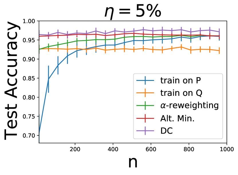
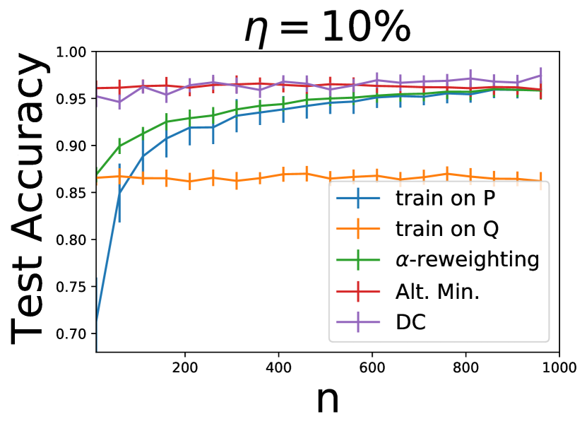
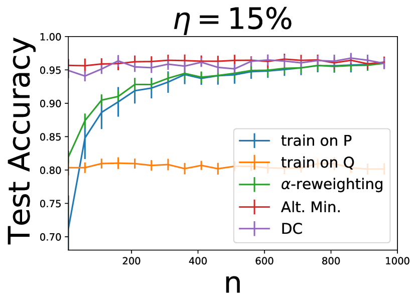
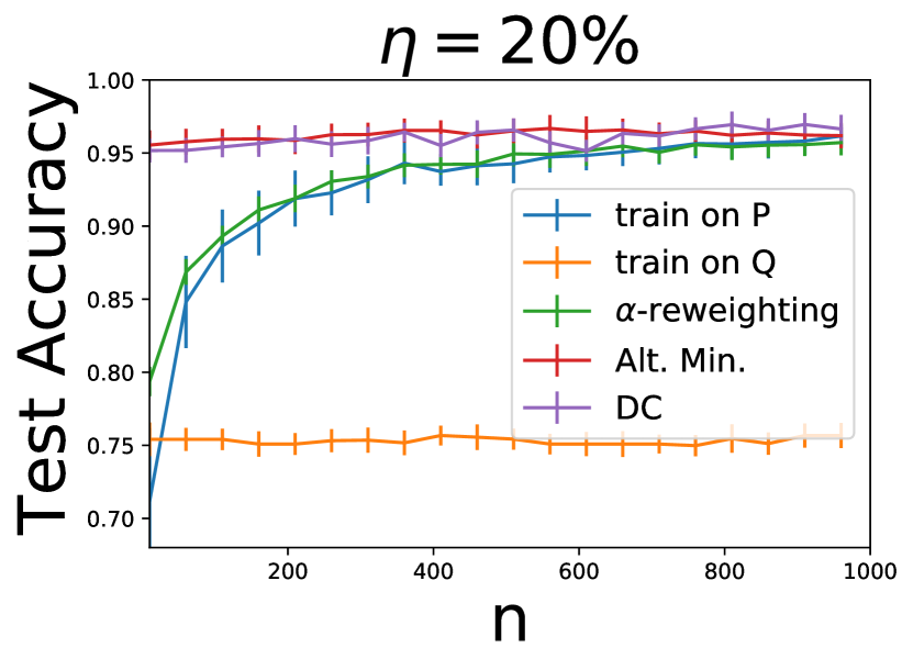
Figure 3: Comparison of sbest against the baselines on simulated data in the classification setting. As the noise rate and therefore the discrepancy between ${\mathscr{P}}$ and ${\mathscr{Q}}$ increases the performance of the baselines degrades. In contrast, both the alternate minimization and the DC-programming algorithms effectively find a good ${\mathsf{q}}$-weighting and can adapt to the target.

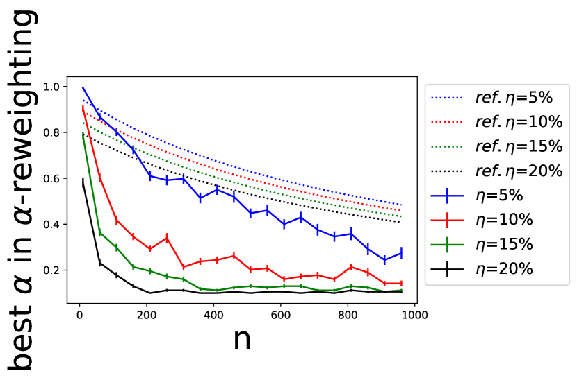
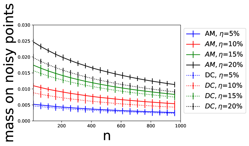
Figure 4: (Left) Best $\alpha$ chosen by $\alpha$-reweighting as a function of $n$. (Right) Total probability mass assigned by sbest to the noisy points.

D.2 Fine-tuning tasks

In this section we demonstrate the effectiveness of our proposed algorithms for the purpose of fine-tuning pre-trained representations. In the standard pre-training/fine-tuning paradigm (Raffel et al., 2019) a model is first pre-trained on a generalist dataset (which is identified as coming from distribution ${\mathscr{Q}}$). Once a good representation is learned, the model is then fine-tuned on a task specific dataset (generated from target ${\mathscr{P}}$). Two of the predominantly used fine-tuning approaches in the literature are last layer fine-tuning (Subramanian et al., 2018; Kiros et al., 2015) and full model fine-tuning (Howard and Ruder, 2018). In the former approach the representations obtained from the last layer of the pre-trained model are used to train a simple model (often a linear hypothesis) on the data coming from ${\mathscr{P}}$. In our experiments we fix the choice of the simple model to be a multi-class logistic regression model. In the latter approach, the model when train on ${\mathscr{P}}$, is initialized from the pre-trained model and all the parameters of the model are fine-tuned (via gradient descent) on the target distribution ${\mathscr{P}}$. In this section we explore the additional advantages of combining data from both ${\mathscr{P}}$ and ${\mathscr{Q}}$ during the fine-tuning stage via our proposed algorithms. There has been recent interest in carefully combining various tasks/data for the purpose of fine-tuning and avoid the phenomenon of “negative transfer” (Aribandi et al., 2021). Our proposed theoretical results present a principled approach towards this.

To evaluate the effectiveness of our theory for this purpose, we consider the CIFAR-10 vision dataset (Krizhevsky et al., 2009). The dataset consists of $50000$ training and $10000$ testing examples belonging to $10$ classes. We form a pre-training task on data from ${\mathscr{Q}}$, by combining all the data belonging to classes: {’airplane’, ’automobile’, ’bird’, ’cat’, ’deer’, ’dog’}. The fine-tuning task consists of data belonging to classes: {’frog’, ’horse’, ’ship’, ’truck’}. We consider both the approaches of last layer fine-tuning and full-model fine-tuning and compare the standard approach of fine-tuning only using data from ${\mathscr{P}}$ with our proposed algorithms. We use $60\%$ of the data from the source for pre-training, and the remaining $40\%$ is used in fine-tuning.

We split the fine-tuning data from ${\mathscr{P}}$ randomly into a $70\%$ training set to be used in fine-tuning, $10\%$ for cross validation and and the remaining $20\%$ to be used as a test set. The results are reported over $5$ such random splits. We perform pre-training on a standard ResNet-18 architecture (He et al., 2016) by optimizing the cross-entropy loss via the Adam optimizer. As can be seen in Table 1 both gapBoost and sbest that combine data from ${\mathscr{P}}$ and ${\mathscr{Q}}$ lead to a classifier with better performance for the downstream task, however, sbest clearly outperforms gapBoost.

The second dataset we consider is the Civil Comments dataset Pavlopoulos et al. (2020). This dataset consists of text comments in online forums and the goal is to predict whether a given comment is toxic or not. Each data point is also labeled with identity terms that describes which subgroup the text in the comment is related to. We create a subsample of the dataset where the target consists of examples from the data points where the identity terms is “asian” and the source is the remaining set of points. This leads to $394,000$ points from the source and $20,000$ points from the target. We create $5$ random splits of the data by randomly partitioning the target data into $10,000$ examples for finetuning, $2000$ for validation and $8000$ for testing. We perform pre-training on a BERT-small model (Devlin et al., 2018) starting from the default checkpoint as obtained from the standard tensorflow implementation of the model.

D.3 Domain adaptation

In this section we evaluate the effectiveness of our proposed best-da objective for adaptation in settings where the target has very little to no labeled data. In order to do this we consider multi-domain sentiment analysis dataset of (Blitzer et al., 2007) that has been used in prior works on domain adaptation. The dataset consists of text reviews associated with a star rating from $1$ to $5$ for various different categories such as books, dvd, etc. We specifically consider four categories namely books, dvd, electronics, and kitchen. Inspired form the methodology adapted in prior works (Mohri and Muñoz Medina, 2012; Cortes and Mohri, 2014), for each category, we form a regression task by converting the review text to a $128$ dimensional vector and fitting a linear regression model to predict the rating. In order to get the features we first combine all the data from the four tasks and convert the raw text to a TF-IDF representation using scikit-learn’s feature extraction library (Pedregosa et al., 2011). Following this, we compute the top $5000$ most important features by using scikit-learn’s feature selection library, that in turn uses a chi-squared test to perform feature selection. Finally, we project the obtained onto a $128$ dimensional space via performing principal component analysis.

After feature extraction, for each task we fit a ridge regression model in the $128$ dimensional space to predict the ratings. The predictions of the model are then defined as the ground truth regression labels. Following the above pre-processing we form 12 adaptation problems for each pair of distinct tasks: (TaskA, TaskB) where TaskA, TaskB are in {books, dvd, electronics, kitchen}. In each case we form the source domain (${\mathscr{Q}}$) by taking $500$ labeled samples from TaskA and $200$ labeled examples from TaskB. The target (${\mathscr{P}}$) is formed by taking $300$ unlabeled examples from TaskB. To our knowledge, there exists no principled method for cross-validation in fully unsupervised domain adaptation. Thus, in our adaptation experiments, we used a small labeled validation set of size $50$ to determine the parameters for all the algorithms. This is consistent with experimental results reported in prior work (e.g., (Cortes and Mohri, 2014)).

We compare our best-da algorithm with the discrepancy minimization (DM) algorithm of Cortes and Mohri (2014), and the (GDM) algorithm, (Cortes et al., 2019b), which is a state of the art adaptation algorithm for regression problems. We also compare with the popular Kernel Mean Matching (KMM) algorithm, (Huang et al., 2006), for domain adaptation. the results averaged over $10$ independent source and target splits, where we normalize the mean squared error (MSE) of best-da to be $1.0$ and present the relative MSE achieved by the other methods. The results show that in most adaptation problems, best-da outperforms (boldface) or ties with (italics) existing methods.

D.3.1 Domain adaptation – covariate-shift

Here we perform experiments for domain adaptation only under covariate shift and compare the performance of our proposed best-da objective with previous state of the art algorithms. We again consider the multi-domain sentiment analysis dataset (Blitzer et al., 2007) from the previous section and in particular focus on the books category. We use the same feature representation as before and define the ground truth as $y=w^{*}\cdot x+\sigma^{2}$ where $w^{*}$ is obtained by fitting a ridge regression classifier. We let the target be the uniform distribution over the entire dataset. We define the source as follows: for a fixed value of $\epsilon$, we pick a random hyperplane $w$ and consider a mixture distribution with mixture weight $0.99$ on the set $w\cdot x\geq\epsilon$ and the mixture weight of $0.01$ on the set $w\cdot x<\epsilon$. The performance of best-da as compared to DM and KMM is shown in Table 2. As can be seen our proposed algorithm either matches or outperforms current algorithms.

Table 2: MSE achieved by best-da as compared to DM and KMM on the covariate shift task for various values of $\epsilon$.

Method	$\epsilon=0$	$\epsilon=0.2$	$\epsilon=0.4$	$\epsilon=0.6$	$\epsilon=0.8$	$\epsilon=1.0$
Train on ${\mathscr{Q}}$	$0.051\pm 0.001$	$0.06\pm 0.001$	$0.06\pm 0.004$	$0.07\pm 0.006$	$0.073\pm 0.002$	$0.073\pm 0.005$
KMM	$0.05\pm 1e-4$	$0.05\pm 1e-4$	$0.05\pm 3e-4$	$0.06\pm 1e-4$	$0.06\pm 1e-4$	$0.07\pm 2e-4$
DM	$0.02\pm 0.005$	$0.06\pm 0.003$	$0.05\pm 0.003$	$0.05\pm 0.001$	$0.06\pm 0.005$	$0.06\pm 0.003$
best-da	$0.01\pm 0.006$	$0.02\pm 0.006$	$0.027\pm 0.005$	$0.04\pm 0.004$	$0.04\pm 0.007$	$0.04\pm 0.004$

Hyperparameters for the algorithms.

For our proposed sbest and sbest-da algorithms the hyperparameters $\lambda_{\infty},\lambda_{1},\lambda_{2}$ were chosen via cross-validation in the union of the sets $\{1e-3,1e-2,1e-1\}$, $\{0,1,2,\dots,10\}$, and $\{0,1000,2000,10000,50000,100000\}$. The $h$ optimization step of alternate minimization was performed using sklearn’s linear regression/logistic regression methods (Pedregosa et al., 2011). During full layer fine-tuning on ResNet/BERT models we use the Adam optimizer for the $h$ optimization step with the default learning rates used for the CIFAR-10 dataset and the BERT-small models.

For the $q$ optimization we used projected gradient descent and the step size was chosen via cross validation in the range $\{1e-3,1e-2,1e-1\}$.

We re-implemented the gapBoost algorithm (Wang et al., 2019a) in Python. Following the prescription by the authors of gapBoost we set the parameter $\gamma=1/n$ where $n$ is the size of the target. We tune parameters $\rho_{S},\rho_{T}$ in the range $\{0.1,0.2,\ldots,1\}$ and the number of rounds of boosting in the range $\{5,10,15,20\}$. We also re-implemented baselines DM (Cortes and Mohri, 2014) and the GDM algorithm (Cortes et al., 2019b). These DM algorithm was implemented via gradient descent and the second stage of the GDM algorithm was implemented via alternate minimization. The learning rates in each case searched in the range $\{1e-3,1e-2,1e-1\}$ and the regularization parameters were searched in the range $\{1e-3,1e-2,1e-1,0,10,100\}$. The radius parameter for GDM was searched in the range $[0.01,1]$ in steps of $0.01$.

To our knowledge, there exists no principled method for cross-validation in fully unsupervised domain adaptation. Thus, in our unsupervised adaptation experiments, we used a small labeled validation set of size $50$ to determine the parameters for all the algorithms. This is consistent with experimental results reported in prior work (Cortes and Mohri, 2014; Cortes et al., 2019b).

References

- Aghajanyan et al. (2021) Armen Aghajanyan, Anchit Gupta, Akshat Shrivastava, Xilun Chen, Luke Zettlemoyer, and Sonal Gupta. Muppet: Massive multi-task representations with pre-finetuning, 2021.
- Aribandi et al. (2021) Vamsi Aribandi, Yi Tay, Tal Schuster, Jinfeng Rao, Huaixiu Steven Zheng, Sanket Vaibhav Mehta, Honglei Zhuang, Vinh Q. Tran, Dara Bahri, Jianmo Ni, Jai Gupta, Kai Hui, Sebastian Ruder, and Donald Metzler. Ext5: Towards extreme multi-task scaling for transfer learning, 2021.
- Balcan et al. (2019) Maria-Florina Balcan, Mikhail Khodak, and Ameet Talwalkar. Provable guarantees for gradient-based meta-learning. In Proceedings of ICML, volume 97, pages 424–433. PMLR, 2019.
- Beck (2015) Amir Beck. On the convergence of alternating minimization for convex programming with applications to iteratively reweighted least squares and decomposition schemes. SIAM J. Optim., 25(1):185–209, 2015.
- Ben-David et al. (2006) Shai Ben-David, John Blitzer, Koby Crammer, and Fernando Pereira. Analysis of representations for domain adaptation. In Proceedings of NIPS, pages 137–144. MIT Press, 2006.
- Ben-David et al. (2010a) Shai Ben-David, John Blitzer, Koby Crammer, Alex Kulesza, Fernando Pereira, and Jennifer Wortman Vaughan. A theory of learning from different domains. Machine learning, 79(1-2):151–175, 2010a.
- Ben-David et al. (2010b) Shai Ben-David, Tyler Lu, Teresa Luu, and Dávid Pál. Impossibility theorems for domain adaptation. Journal of Machine Learning Research - Proceedings Track, 9:129–136, 2010b.
- Berlind and Urner (2015) Christopher Berlind and Ruth Urner. Active nearest neighbors in changing environments. In Proceedings of ICML, volume 37, pages 1870–1879. JMLR.org, 2015.
- Blanchard et al. (2011) Gilles Blanchard, Gyemin Lee, and Clayton Scott. Generalizing from several related classification tasks to a new unlabeled sample. In NIPS, pages 2178–2186, 2011.
- Blitzer et al. (2007) John Blitzer, Mark Dredze, and Fernando Pereira. Biographies, bollywood, boom-boxes and blenders: Domain adaptation for sentiment classification. In Proceedings of ACL, pages 440–447, 2007.
- Blitzer et al. (2008) John Blitzer, Koby Crammer, Alex Kulesza, Fernando Pereira, and Jennifer Wortman. Learning bounds for domain adaptation. In Proceedings of NIPS, pages 129–136, 2008.
- Bousmalis et al. (2017) Konstantinos Bousmalis, Nathan Silberman, David Dohan, Dumitru Erhan, and Dilip Krishnan. Unsupervised pixel-level domain adaptation with generative adversarial networks. In Proceedings of the IEEE conference on computer vision and pattern recognition, pages 3722–3731, 2017.
- Chattopadhyay et al. (2013) Rita Chattopadhyay, Wei Fan, Ian Davidson, Sethuraman Panchanathan, and Jieping Ye. Joint transfer and batch-mode active learning. In Proceedings of ICML, volume 28, pages 253–261. JMLR.org, 2013.
- Chen et al. (2011) Minmin Chen, Kilian Q Weinberger, and John Blitzer. Co-training for domain adaptation. In Nips, volume 24, pages 2456–2464. Citeseer, 2011.
- Chen et al. (2017) Robert S Chen, Brendan Lucier, Yaron Singer, and Vasilis Syrgkanis. Robust optimization for non-convex objectives. In Advances in Neural Information Processing Systems, pages 4705–4714, 2017.
- Cortes and Mohri (2011) Corinna Cortes and Mehryar Mohri. Domain adaptation in regression. In Proceedings of ALT, pages 308–323, 2011.
- Cortes and Mohri (2014) Corinna Cortes and Mehryar Mohri. Domain adaptation and sample bias correction theory and algorithm for regression. Theor. Comput. Sci., 519:103–126, 2014.
- Cortes et al. (2010) Corinna Cortes, Yishay Mansour, and Mehryar Mohri. Learning bounds for importance weighting. In Proceedings of NIPS, pages 442–450. Curran Associates, Inc., 2010.
- Cortes et al. (2019a) Corinna Cortes, Spencer Greenberg, and Mehryar Mohri. Relative deviation learning bounds and generalization with unbounded loss functions. Ann. Math. Artif. Intell., 85(1):45–70, 2019a.
- Cortes et al. (2019b) Corinna Cortes, Mehryar Mohri, and Andrés Muñoz Medina. Adaptation based on generalized discrepancy. J. Mach. Learn. Res., 20:1:1–1:30, 2019b.
- Cortes et al. (2021) Corinna Cortes, Mehryar Mohri, Ananda Theertha Suresh, and Ningshan Zhang. A discriminative technique for multiple-source adaptation. In Marina Meila and Tong Zhang, editors, Proceedings of the 38th International Conference on Machine Learning, ICML 2021, 18-24 July 2021, Virtual Event, volume 139 of Proceedings of Machine Learning Research, pages 2132–2143. PMLR, 2021.
- Courty et al. (2016) Nicolas Courty, Rémi Flamary, Devis Tuia, and Alain Rakotomamonjy. Optimal transport for domain adaptation. IEEE transactions on pattern analysis and machine intelligence, 39(9):1853–1865, 2016.
- Courty et al. (2017) Nicolas Courty, Rémi Flamary, Devis Tuia, and Alain Rakotomamonjy. Optimal transport for domain adaptation. IEEE Trans. Pattern Anal. Mach. Intell., 39(9):1853–1865, 2017.
- Crammer et al. (2008) Koby Crammer, Michael J. Kearns, and Jennifer Wortman. Learning from multiple sources. Journal of Machine Learning Research, 9(Aug):1757–1774, 2008.
- Daumé III (2007) Hal Daumé III. Frustratingly easy domain adaptation. ACL 2007, page 256, 2007.
- de Mathelin et al. (2021) Antoine de Mathelin, Mathilde Mougeot, and Nicolas Vayatis. Discrepancy-based active learning for domain adaptation. CoRR, abs/2103.03757, 2021.
- Devlin et al. (2018) Jacob Devlin, Ming-Wei Chang, Kenton Lee, and Kristina Toutanova. Bert: Pre-training of deep bidirectional transformers for language understanding. arXiv preprint arXiv:1810.04805, 2018.
- Du et al. (2017) Simon S. Du, Jayanth Koushik, Aarti Singh, and Barnabás Póczos. Hypothesis transfer learning via transformation functions. In Isabelle Guyon, Ulrike von Luxburg, Samy Bengio, Hanna M. Wallach, Rob Fergus, S. V. N. Vishwanathan, and Roman Garnett, editors, Advances in Neural Information Processing Systems 30: Annual Conference on Neural Information Processing Systems 2017, December 4-9, 2017, Long Beach, CA, USA, pages 574–584, 2017.
- Duan et al. (2009) Lixin Duan, Ivor W. Tsang, Dong Xu, and Tat-Seng Chua. Domain adaptation from multiple sources via auxiliary classifiers. In ICML, volume 382, pages 289–296, 2009.
- Duan et al. (2012) Lixin Duan, Dong Xu, and Ivor Wai-Hung Tsang. Domain adaptation from multiple sources: A domain-dependent regularization approach. IEEE Transactions on Neural Networks and Learning Systems, 23(3):504–518, 2012.
- Fernando et al. (2013) Basura Fernando, Amaury Habrard, Marc Sebban, and Tinne Tuytelaars. Unsupervised visual domain adaptation using subspace alignment. In Proceedings of the IEEE international conference on computer vision, pages 2960–2967, 2013.
- Finn et al. (2017) Chelsea Finn, Pieter Abbeel, and Sergey Levine. Model-agnostic meta-learning for fast adaptation of deep networks. In Doina Precup and Yee Whye Teh, editors, Proceedings of the 34th International Conference on Machine Learning, ICML 2017, Sydney, NSW, Australia, 6-11 August 2017, volume 70 of Proceedings of Machine Learning Research, pages 1126–1135. PMLR, 2017.
- Gan et al. (2016) Chuang Gan, Tianbao Yang, and Boqing Gong. Learning attributes equals multi-source domain generalization. In Proceedings of the IEEE conference on computer vision and pattern recognition, pages 87–97, 2016.
- Ganin et al. (2016) Yaroslav Ganin, Evgeniya Ustinova, Hana Ajakan, Pascal Germain, Hugo Larochelle, François Laviolette, Mario Marchand, and Victor Lempitsky. Domain-adversarial training of neural networks. The Journal of Machine Learning Research, 17(1):2096–2030, 2016.
- Garcke and Vanck (2014) Jochen Garcke and Thomas Vanck. Importance weighted inductive transfer learning for regression. In Toon Calders, Floriana Esposito, Eyke Hüllermeier, and Rosa Meo, editors, Proceedings of ECML, volume 8724 of Lecture Notes in Computer Science, pages 466–481. Springer, 2014.
- Germain et al. (2013) Pascal Germain, Amaury Habrard, François Laviolette, and Emilie Morvant. A PAC-bayesian approach for domain adaptation with specialization to linear classifiers. In Proceedings of the 30th International Conference on Machine Learning, ICML 2013, Atlanta, GA, USA, 16-21 June 2013, volume 28 of JMLR Workshop and Conference Proceedings, pages 738–746. JMLR.org, 2013.
- Ghifary et al. (2015) Muhammad Ghifary, W Bastiaan Kleijn, Mengjie Zhang, and David Balduzzi. Domain generalization for object recognition with multi-task autoencoders. In Proceedings of the IEEE international conference on computer vision, pages 2551–2559, 2015.
- Ghifary et al. (2016a) Muhammad Ghifary, David Balduzzi, W Bastiaan Kleijn, and Mengjie Zhang. Scatter component analysis: A unified framework for domain adaptation and domain generalization. IEEE transactions on pattern analysis and machine intelligence, 39(7):1414–1430, 2016a.
- Ghifary et al. (2016b) Muhammad Ghifary, W Bastiaan Kleijn, Mengjie Zhang, David Balduzzi, and Wen Li. Deep reconstruction-classification networks for unsupervised domain adaptation. In European conference on computer vision, pages 597–613. Springer, 2016b.
- Gong et al. (2012) Boqing Gong, Yuan Shi, Fei Sha, and Kristen Grauman. Geodesic flow kernel for unsupervised domain adaptation. In CVPR, pages 2066–2073, 2012.
- Gong et al. (2013a) Boqing Gong, Kristen Grauman, and Fei Sha. Connecting the dots with landmarks: Discriminatively learning domain-invariant features for unsupervised domain adaptation. In ICML, volume 28, pages 222–230, 2013a.
- Gong et al. (2013b) Boqing Gong, Kristen Grauman, and Fei Sha. Reshaping visual datasets for domain adaptation. In NIPS, pages 1286–1294, 2013b.
- Gong et al. (2016) Mingming Gong, Kun Zhang, Tongliang Liu, Dacheng Tao, Clark Glymour, and Bernhard Schölkopf. Domain adaptation with conditional transferable components. In Maria-Florina Balcan and Kilian Q. Weinberger, editors, Proceedings of the 33nd International Conference on Machine Learning, ICML 2016, New York City, NY, USA, June 19-24, 2016, volume 48 of JMLR Workshop and Conference Proceedings, pages 2839–2848. JMLR.org, 2016.
- Grippo and Sciandrone (2000) Luigi Grippo and Marco Sciandrone. On the convergence of the block nonlinear gauss-seidel method under convex constraints. Oper. Res. Lett., 26(3):127–136, 2000.
- Guo et al. (2019) Yunhui Guo, Honghui Shi, Abhishek Kumar, Kristen Grauman, Tajana Rosing, and Rogerio Feris. Spottune: Transfer learning through adaptive fine-tuning. In Proceedings of the IEEE/CVF Conference on Computer Vision and Pattern Recognition (CVPR), June 2019.
- Hanneke and Kpotufe (2019) Steve Hanneke and Samory Kpotufe. On the value of target data in transfer learning. In Hanna M. Wallach, Hugo Larochelle, Alina Beygelzimer, Florence d’Alché-Buc, Emily B. Fox, and Roman Garnett, editors, Advances in Neural Information Processing Systems 32: Annual Conference on Neural Information Processing Systems 2019, NeurIPS 2019, December 8-14, 2019, Vancouver, BC, Canada, pages 9867–9877, 2019.
- He et al. (2016) Kaiming He, Xiangyu Zhang, Shaoqing Ren, and Jian Sun. Deep residual learning for image recognition. In Proceedings of the IEEE conference on computer vision and pattern recognition, pages 770–778, 2016.
- Hedegaard et al. (2021) Lukas Hedegaard, Omar Ali Sheikh-Omar, and Alexandros Iosifidis. Supervised domain adaptation: A graph embedding perspective and a rectified experimental protocol. IEEE Trans. Image Process., 30:8619–8631, 2021.
- Hoffman et al. (2012) Judy Hoffman, Brian Kulis, Trevor Darrell, and Kate Saenko. Discovering latent domains for multisource domain adaptation. In ECCV, volume 7573, pages 702–715, 2012.
- Hoffman et al. (2018) Judy Hoffman, Mehryar Mohri, and Ningshan Zhang. Algorithms and theory for multiple-source adaptation. In Proceedings of NeurIPS, pages 8256–8266, 2018.
- Hoffman et al. (2021) Judy Hoffman, Mehryar Mohri, and Ningshan Zhang. Multiple-source adaptation theory and algorithms. Annals of Mathematics and Artificial Intelligence, 89(3-4):237–270, 2021.
- Hoffman et al. (2022) Judy Hoffman, Mehryar Mohri, and Ningshan Zhang. Multiple-source adaptation theory and algorithms - addendum. Annals of Mathematics and Artificial Intelligence, 90(6):569–572, 2022.
- Horst and Thoai (1999) R Horst and Nguyen V Thoai. DC programming: overview. Journal of Optimization Theory and Applications, 103(1):1–43, 1999.
- Houlsby et al. (2019) Neil Houlsby, Andrei Giurgiu, Stanislaw Jastrzebski, Bruna Morrone, Quentin de Laroussilhe, Andrea Gesmundo, Mona Attariyan, and Sylvain Gelly. Parameter-efficient transfer learning for NLP. CoRR, abs/1902.00751, 2019. URL http://arxiv.org/abs/1902.00751.
- Howard and Ruder (2018) Jeremy Howard and Sebastian Ruder. Universal language model fine-tuning for text classification. In Proceedings of the 56th Annual Meeting of the Association for Computational Linguistics (Volume 1: Long Papers), pages 328–339, Melbourne, Australia, July 2018. Association for Computational Linguistics. 10.18653/v1/P18-1031. URL https://aclanthology.org/P18-1031.
- Huang et al. (2006) Jiayuan Huang, Alexander J. Smola, Arthur Gretton, Karsten M. Borgwardt, and Bernhard Schölkopf. Correcting sample selection bias by unlabeled data. In NIPS 2006, volume 19, pages 601–608, 2006.
- Huang et al. (2017) Xingchang Huang, Yanghui Rao, Haoran Xie, Tak-Lam Wong, and Fu Lee Wang. Cross-domain sentiment classification via topic-related tradaboost. In Thirty-First AAAI Conference on Artificial Intelligence, 2017.
- Jhuo et al. (2012) I-Hong Jhuo, Dong Liu, DT Lee, and Shih-Fu Chang. Robust visual domain adaptation with low-rank reconstruction. In 2012 IEEE conference on computer vision and pattern recognition, pages 2168–2175. IEEE, 2012.
- Khosla et al. (2012) Aditya Khosla, Tinghui Zhou, Tomasz Malisiewicz, Alexei A. Efros, and Antonio Torralba. Undoing the damage of dataset bias. In ECCV, volume 7572, pages 158–171, 2012.
- Kifer et al. (2004) Daniel Kifer, Shai Ben-David, and Johannes Gehrke. Detecting change in data streams. In Mario A. Nascimento, M. Tamer Özsu, Donald Kossmann, Renée J. Miller, José A. Blakeley, and K. Bernhard Schiefer, editors, (e)Proceedings of the Thirtieth International Conference on Very Large Data Bases, VLDB 2004, Toronto, Canada, August 31 - September 3 2004, pages 180–191. Morgan Kaufmann, 2004.
- Kiros et al. (2015) Ryan Kiros, Yukun Zhu, Russ R Salakhutdinov, Richard Zemel, Raquel Urtasun, Antonio Torralba, and Sanja Fidler. Skip-thought vectors. In Advances in neural information processing systems, pages 3294–3302, 2015.
- Koenecke et al. (2020) Allison Koenecke, Andrew Nam, Emily Lake, Joe Nudell, Minnie Quartey, Zion Mengesha, Connor Toups, John R. Rickford, Dan Jurafsky, and Sharad Goel. Racial disparities in automated speech recognition. Proc. Natl. Acad. Sci. USA, 117(14):7684–7689, 2020.
- Konstantinov and Lampert (2019) Nikola Konstantinov and Christoph Lampert. Robust learning from untrusted sources. In International Conference on Machine Learning, pages 3488–3498, 2019.
- Kpotufe and Martinet (2018) Samory Kpotufe and Guillaume Martinet. Marginal singularity, and the benefits of labels in covariate-shift. In Sébastien Bubeck, Vianney Perchet, and Philippe Rigollet, editors, Conference On Learning Theory, COLT 2018, Stockholm, Sweden, 6-9 July 2018, volume 75 of Proceedings of Machine Learning Research, pages 1882–1886. PMLR, 2018.
- Krizhevsky et al. (2009) Alex Krizhevsky, Geoffrey Hinton, et al. Learning multiple layers of features from tiny images. Technical report, Toronto University, 2009.
- Kundu et al. (2020) Jogendra Nath Kundu, Naveen Venkat, R Venkatesh Babu, et al. Universal source-free domain adaptation. In Proceedings of the IEEE/CVF Conference on Computer Vision and Pattern Recognition, pages 4544–4553, 2020.
- Kuzborskij and Orabona (2013) Ilja Kuzborskij and Francesco Orabona. Stability and hypothesis transfer learning. In Proceedings of the 30th International Conference on Machine Learning, ICML 2013, Atlanta, GA, USA, 16-21 June 2013, volume 28 of JMLR Workshop and Conference Proceedings, pages 942–950. JMLR.org, 2013.
- Ledoux and Talagrand (1991) Michel Ledoux and Michel Talagrand. Probability in Banach Spaces: Isoperimetry and Processes. Springer, New York, 1991.
- Li et al. (2018) Jingjing Li, Ke Lu, Zi Huang, Lei Zhu, and Heng Tao Shen. Transfer independently together: A generalized framework for domain adaptation. IEEE transactions on cybernetics, 49(6):2144–2155, 2018.
- Li (2012) Qi Li. Literature survey: domain adaptation algorithms for natural language processing. Department of Computer Science The Graduate Center, The City University of New York, pages 8–10, 2012.
- Li et al. (2019) Qiuwei Li, Zhihui Zhu, and Gongguo Tang. Alternating minimizations converge to second-order optimal solutions. In Kamalika Chaudhuri and Ruslan Salakhutdinov, editors, Proceedings of the 36th International Conference on Machine Learning, ICML 2019, 9-15 June 2019, Long Beach, California, USA, volume 97 of Proceedings of Machine Learning Research, pages 3935–3943. PMLR, 2019.
- Liu et al. (2016) Hongfu Liu, Ming Shao, and Yun Fu. Structure-preserved multi-source domain adaptation. In 2016 IEEE 16th International Conference on Data Mining (ICDM), pages 1059–1064. IEEE, 2016.
- Long et al. (2015) Mingsheng Long, Yue Cao, Jianmin Wang, and Michael I. Jordan. Learning transferable features with deep adaptation networks. In Francis R. Bach and David M. Blei, editors, Proceedings of the 32nd International Conference on Machine Learning, ICML 2015, Lille, France, 6-11 July 2015, volume 37 of JMLR Workshop and Conference Proceedings, pages 97–105. JMLR.org, 2015.
- Long et al. (2016) Mingsheng Long, Han Zhu, Jianmin Wang, and Michael I Jordan. Unsupervised domain adaptation with residual transfer networks. arXiv preprint arXiv:1602.04433, 2016.
- Lu et al. (2021) Nan Lu, Tianyi Zhang, Tongtong Fang, Takeshi Teshima, and Masashi Sugiyama. Rethinking importance weighting for transfer learning. CoRR, abs/2112.10157, 2021. URL https://arxiv.org/abs/2112.10157.
- Mansour et al. (2009a) Yishay Mansour, Mehryar Mohri, and Afshin Rostamizadeh. Domain adaptation: Learning bounds and algorithms. In COLT 2009 - The 22nd Conference on Learning Theory, Montreal, Quebec, Canada, June 18-21, 2009, 2009a.
- Mansour et al. (2009b) Yishay Mansour, Mehryar Mohri, and Afshin Rostamizadeh. Domain adaptation with multiple sources. In NIPS, pages 1041–1048, 2009b.
- Mansour et al. (2021) Yishay Mansour, Mehryar Mohri, Jae Ro, Ananda Theertha Suresh, and Ke Wu. A theory of multiple-source adaptation with limited target labeled data. In Arindam Banerjee and Kenji Fukumizu, editors, The 24th International Conference on Artificial Intelligence and Statistics, AISTATS 2021, April 13-15, 2021, Virtual Event, volume 130 of Proceedings of Machine Learning Research, pages 2332–2340. PMLR, 2021.
- Maurer (2006) Andreas Maurer. Bounds for linear multi-task learning. J. Mach. Learn. Res., 7:117–139, 2006.
- Maurer et al. (2016) Andreas Maurer, Massimiliano Pontil, and Bernardino Romera-Paredes. The benefit of multitask representation learning. J. Mach. Learn. Res., 17:81:1–81:32, 2016.
- Mohri and Muñoz Medina (2012) Mehryar Mohri and Andres Muñoz Medina. New analysis and algorithm for learning with drifting distributions. In Nader H. Bshouty, Gilles Stoltz, Nicolas Vayatis, and Thomas Zeugmann, editors, Algorithmic Learning Theory - 23rd International Conference, ALT 2012, Lyon, France, October 29-31, 2012. Proceedings, volume 7568 of Lecture Notes in Computer Science, pages 124–138. Springer, 2012.
- Mohri et al. (2018) Mehryar Mohri, Afshin Rostamizadeh, and Ameet Talwalkar. Foundations of Machine Learning. MIT Press, second edition, 2018.
- Mohri et al. (2019) Mehryar Mohri, Gary Sivek, and Ananda Theertha Suresh. Agnostic federated learning. In International Conference on Machine Learning, pages 4615–4625. PMLR, 2019.
- Motiian et al. (2017a) Saeid Motiian, Quinn Jones, Seyed Iranmanesh, and Gianfranco Doretto. Few-shot adversarial domain adaptation. In Advances in Neural Information Processing Systems, pages 6670–6680, 2017a.
- Motiian et al. (2017b) Saeid Motiian, Marco Piccirilli, Donald A Adjeroh, and Gianfranco Doretto. Unified deep supervised domain adaptation and generalization. In Proceedings of the IEEE International Conference on Computer Vision, pages 5715–5725, 2017b.
- Muandet et al. (2013) Krikamol Muandet, David Balduzzi, and Bernhard Schölkopf. Domain generalization via invariant feature representation. In ICML, volume 28, pages 10–18, 2013.
- Nichol et al. (2018) Alex Nichol, Joshua Achiam, and John Schulman. On first-order meta-learning algorithms. CoRR, abs/1803.02999, 2018. URL http://arxiv.org/abs/1803.02999.
- Pan and Yang (2009) Sinno Jialin Pan and Qiang Yang. A survey on transfer learning. IEEE Transactions on knowledge and data engineering, 22(10):1345–1359, 2009.
- Pavlopoulos et al. (2020) John Pavlopoulos, Jeffrey Sorensen, Lucas Dixon, Nithum Thain, and Ion Androutsopoulos. Toxicity detection: Does context really matter?, 2020.
- Pedregosa et al. (2011) F. Pedregosa, G. Varoquaux, A. Gramfort, V. Michel, B. Thirion, O. Grisel, M. Blondel, P. Prettenhofer, R. Weiss, V. Dubourg, J. Vanderplas, A. Passos, D. Cournapeau, M. Brucher, M. Perrot, and E. Duchesnay. Scikit-learn: Machine learning in Python. Journal of Machine Learning Research, 12:2825–2830, 2011.
- Pei et al. (2018) Zhongyi Pei, Zhangjie Cao, Mingsheng Long, and Jianmin Wang. Multi-adversarial domain adaptation. In AAAI, pages 3934–3941, 2018.
- Peng et al. (2019) Xingchao Peng, Qinxun Bai, Xide Xia, Zijun Huang, Kate Saenko, and Bo Wang. Moment matching for multi-source domain adaptation. In Proceedings of the IEEE International Conference on Computer Vision, pages 1406–1415, 2019.
- Pentina and Ben-David (2018) Anastasia Pentina and Shai Ben-David. Multi-task Kernel Learning based on Probabilistic Lipschitzness. In Firdaus Janoos, Mehryar Mohri, and Karthik Sridharan, editors, Algorithmic Learning Theory, ALT 2018, 7-9 April 2018, Lanzarote, Canary Islands, Spain, volume 83 of Proceedings of Machine Learning Research, pages 682–701. PMLR, 2018.
- Pentina and Lampert (2014) Anastasia Pentina and Christoph H. Lampert. A PAC-bayesian bound for lifelong learning. In Proceedings of the 31th International Conference on Machine Learning, ICML 2014, Beijing, China, 21-26 June 2014, volume 32 of JMLR Workshop and Conference Proceedings, pages 991–999. JMLR.org, 2014.
- Pentina and Lampert (2015) Anastasia Pentina and Christoph H. Lampert. Lifelong learning with non-i.i.d. tasks. In Corinna Cortes, Neil D. Lawrence, Daniel D. Lee, Masashi Sugiyama, and Roman Garnett, editors, Advances in Neural Information Processing Systems 28: Annual Conference on Neural Information Processing Systems 2015, December 7-12, 2015, Montreal, Quebec, Canada, pages 1540–1548, 2015.
- Pentina and Lampert (2017) Anastasia Pentina and Christoph H. Lampert. Multi-task learning with labeled and unlabeled tasks. In Doina Precup and Yee Whye Teh, editors, Proceedings of the 34th International Conference on Machine Learning, ICML 2017, Sydney, NSW, Australia, 6-11 August 2017, volume 70 of Proceedings of Machine Learning Research, pages 2807–2816. PMLR, 2017.
- Pentina and Urner (2016) Anastasia Pentina and Ruth Urner. Lifelong learning with weighted majority votes. In Daniel D. Lee, Masashi Sugiyama, Ulrike von Luxburg, Isabelle Guyon, and Roman Garnett, editors, Advances in Neural Information Processing Systems 29: Annual Conference on Neural Information Processing Systems 2016, December 5-10, 2016, Barcelona, Spain, pages 3612–3620, 2016.
- Perrot and Habrard (2015) Michaël Perrot and Amaury Habrard. A theoretical analysis of metric hypothesis transfer learning. In Francis R. Bach and David M. Blei, editors, Proceedings of the 32nd International Conference on Machine Learning, ICML 2015, Lille, France, 6-11 July 2015, volume 37 of JMLR Workshop and Conference Proceedings, pages 1708–1717. JMLR.org, 2015.
- Peters et al. (2018) Matthew E. Peters, Mark Neumann, Mohit Iyyer, Matt Gardner, Christopher Clark, Kenton Lee, and Luke Zettlemoyer. Deep contextualized word representations. In Proceedings of the 2018 Conference of the North American Chapter of the Association for Computational Linguistics: Human Language Technologies, Volume 1 (Long Papers), pages 2227–2237, New Orleans, Louisiana, June 2018. Association for Computational Linguistics. 10.18653/v1/N18-1202. URL https://aclanthology.org/N18-1202.
- Raffel et al. (2019) Colin Raffel, Noam Shazeer, Adam Roberts, Katherine Lee, Sharan Narang, Michael Matena, Yanqi Zhou, Wei Li, and Peter J Liu. Exploring the limits of transfer learning with a unified text-to-text transformer. arXiv preprint arXiv:1910.10683, 2019.
- Redko and Bennani (2016) Ievgen Redko and Younès Bennani. Non-negative embedding for fully unsupervised domain adaptation. Pattern Recognit. Lett., 77:35–41, 2016.
- Redko et al. (2017) Ievgen Redko, Amaury Habrard, and Marc Sebban. Theoretical analysis of domain adaptation with optimal transport. In Michelangelo Ceci, Jaakko Hollmén, Ljupco Todorovski, Celine Vens, and Saso Dzeroski, editors, Machine Learning and Knowledge Discovery in Databases - European Conference, ECML PKDD 2017, Skopje, Macedonia, September 18-22, 2017, Proceedings, Part II, volume 10535 of Lecture Notes in Computer Science, pages 737–753. Springer, 2017.
- Saito et al. (2018) Kuniaki Saito, Kohei Watanabe, Yoshitaka Ushiku, and Tatsuya Harada. Maximum classifier discrepancy for unsupervised domain adaptation. In Proceedings of the IEEE conference on computer vision and pattern recognition, pages 3723–3732, 2018.
- Saito et al. (2019) Kuniaki Saito, Donghyun Kim, Stan Sclaroff, Trevor Darrell, and Kate Saenko. Semi-supervised domain adaptation via minimax entropy. In Proceedings of the IEEE International Conference on Computer Vision, pages 8050–8058, 2019.
- Sener et al. (2016) Ozan Sener, Hyun Oh Song, Ashutosh Saxena, and Silvio Savarese. Learning transferrable representations for unsupervised domain adaptation. In Advances in Neural Information Processing Systems, pages 2110–2118, 2016.
- Sriperumbudur et al. (2007) Bharath K. Sriperumbudur, David A. Torres, and Gert R. G. Lanckriet. Sparse eigen methods by D.C. programming. In ICML, pages 831–838, 2007.
- Subramanian et al. (2018) Sandeep Subramanian, Adam Trischler, Yoshua Bengio, and Christopher J Pal. Learning general purpose distributed sentence representations via large scale multi-task learning. arXiv preprint arXiv:1804.00079, 2018.
- Sugiyama et al. (2007a) Masashi Sugiyama, Matthias Krauledat, and Klaus-Robert Müller. Covariate shift adaptation by importance weighted cross validation. volume 8, pages 985–1005, 2007a.
- Sugiyama et al. (2007b) Masashi Sugiyama, Shinichi Nakajima, Hisashi Kashima, Paul von Bünau, and Motoaki Kawanabe. Direct importance estimation with model selection and its application to covariate shift adaptation. In John C. Platt, Daphne Koller, Yoram Singer, and Sam T. Roweis, editors, Advances in Neural Information Processing Systems 20, Proceedings of the Twenty-First Annual Conference on Neural Information Processing Systems, Vancouver, British Columbia, Canada, December 3-6, 2007, pages 1433–1440. Curran Associates, Inc., 2007b.
- Sun and Saenko (2016) Baochen Sun and Kate Saenko. Deep coral: Correlation alignment for deep domain adaptation. In European conference on computer vision, pages 443–450. Springer, 2016.
- Sun et al. (2016) Baochen Sun, Jiashi Feng, and Kate Saenko. Return of frustratingly easy domain adaptation. In Proceedings of the AAAI Conference on Artificial Intelligence, volume 30, 2016.
- Sun et al. (2011) Qian Sun, Rita Chattopadhyay, Sethuraman Panchanathan, and Jieping Ye. A two-stage weighting framework for multi-source domain adaptation. In Advances in neural information processing systems, pages 505–513, 2011.
- Tao and An (1997) Pham Dinh Tao and Le Thi Hoai An. Convex analysis approach to DC programming: theory, algorithms and applications. Acta Mathematica Vietnamica, 22(1):289–355, 1997.
- Tao and An (1998) Pham Dinh Tao and Le Thi Hoai An. A DC optimization algorithm for solving the trust-region subproblem. SIAM Journal on Optimization, 8(2):476–505, 1998.
- Tuy (1964) Hoang Tuy. Concave programming under linear constraints. Translated Soviet Mathematics, 5:1437–1440, 1964.
- Tzeng et al. (2015) Eric Tzeng, Judy Hoffman, Trevor Darrell, and Kate Saenko. Simultaneous deep transfer across domains and tasks. In Proceedings of the IEEE International Conference on Computer Vision, pages 4068–4076, 2015.
- Wang et al. (2019a) Boyu Wang, Jorge A. Mendez, Mingbo Cai, and Eric Eaton. Transfer learning via minimizing the performance gap between domains. In Proceedingz of NeurIPS, pages 10644–10654, 2019a.
- Wang and Mahadevan (2011) Chang Wang and Sridhar Mahadevan. Heterogeneous domain adaptation using manifold alignment. In Twenty-second international joint conference on artificial intelligence, 2011.
- Wang et al. (2018) Jindong Wang, Wenjie Feng, Yiqiang Chen, Han Yu, Meiyu Huang, and Philip S Yu. Visual domain adaptation with manifold embedded distribution alignment. In Proceedings of the 26th ACM international conference on Multimedia, pages 402–410, 2018.
- Wang and Deng (2018) Mei Wang and Weihong Deng. Deep visual domain adaptation: A survey. Neurocomputing, 312:135–153, 2018.
- Wang et al. (2019b) Tao Wang, Xiaopeng Zhang, Li Yuan, and Jiashi Feng. Few-shot adaptive faster r-cnn. In Proceedings of the IEEE Conference on Computer Vision and Pattern Recognition, pages 7173–7182, 2019b.
- Wei et al. (2021) Jason Wei, Maarten Bosma, Vincent Y. Zhao, Kelvin Guu, Adams Wei Yu, Brian Lester, Nan Du, Andrew M. Dai, and Quoc V. Le. Finetuned language models are zero-shot learners, 2021.
- Wen et al. (2020) Junfeng Wen, Russell Greiner, and Dale Schuurmans. Domain aggregation networks for multi-source domain adaptation. In International Conference on Machine Learning, pages 10214–10224. PMLR, 2020.
- Yang et al. (2007) Jun Yang, Rong Yan, and Alexander G. Hauptmann. Cross-domain video concept detection using adaptive svms. In ACM Multimedia, pages 188–197, 2007.
- Yang et al. (2013) Liu Yang, Steve Hanneke, and Jaime G. Carbonell. A theory of transfer learning with applications to active learning. Mach. Learn., 90(2):161–189, 2013.
- You et al. (2020) Kaichao You, Zhi Kou, Mingsheng Long, and Jianmin Wang. Co-tuning for transfer learning. Advances in Neural Information Processing Systems, 33, 2020.
- Yuille and Rangarajan (2003) Alan L. Yuille and Anand Rangarajan. The concave-convex procedure. Neural Computation, 15(4):915–936, 2003.
- Zhang et al. (2013) Kun Zhang, Bernhard Schölkopf, Krikamol Muandet, and Zhikun Wang. Domain adaptation under target and conditional shift. In Proceedings of the 30th International Conference on Machine Learning, ICML 2013, Atlanta, GA, USA, 16-21 June 2013, volume 28 of JMLR Workshop and Conference Proceedings, pages 819–827. JMLR.org, 2013.
- Zhang et al. (2020a) Tianyi Zhang, Ikko Yamane, Nan Lu, and Masashi Sugiyama. A one-step approach to covariate shift adaptation. In Proceedings of ACML, volume 129 of Proceedings of Machine Learning Research, pages 65–80. PMLR, 2020a.
- Zhang et al. (2019a) Yuchen Zhang, Tianle Liu, Mingsheng Long, and Michael Jordan. Bridging theory and algorithm for domain adaptation. In Kamalika Chaudhuri and Ruslan Salakhutdinov, editors, Proceedings of the 36th International Conference on Machine Learning, volume 97 of Proceedings of Machine Learning Research, pages 7404–7413. PMLR, 09–15 Jun 2019a.
- Zhang et al. (2019b) Yuchen Zhang, Tianle Liu, Mingsheng Long, and Michael Jordan. Bridging theory and algorithm for domain adaptation. In International Conference on Machine Learning, pages 7404–7413. PMLR, 2019b.
- Zhang et al. (2019c) Yuchen Zhang, Tianle Liu, Mingsheng Long, and Michael I. Jordan. Bridging theory and algorithm for domain adaptation. In Kamalika Chaudhuri and Ruslan Salakhutdinov, editors, Proceedings of the 36th International Conference on Machine Learning, ICML 2019, 9-15 June 2019, Long Beach, California, USA, volume 97 of Proceedings of Machine Learning Research, pages 7404–7413. PMLR, 2019c.
- Zhang et al. (2020b) Yuchen Zhang, Mingsheng Long, Jianmin Wang, and Michael I. Jordan. On localized discrepancy for domain adaptation. CoRR, abs/2008.06242, 2020b.
- Zhao et al. (2018) Han Zhao, Shanghang Zhang, Guanhang Wu, José MF Moura, Joao P Costeira, and Geoffrey J Gordon. Adversarial multiple source domain adaptation. Advances in neural information processing systems, 31:8559–8570, 2018.
- Zhao et al. (2019) Han Zhao, Remi Tachet Des Combes, Kun Zhang, and Geoffrey Gordon. On learning invariant representations for domain adaptation. In International Conference on Machine Learning, pages 7523–7532. PMLR, 2019.
- Zheng et al. (2020) Lutao Zheng, Guanjun Liu, Chungang Yan, Changjun Jiang, Mengchu Zhou, and Maozhen Li. Improved tradaboost and its application to transaction fraud detection. IEEE Transactions on Computational Social Systems, 7(5):1304–1316, 2020.