$\mathcal{PT}$ -Symmetric Quantum Field Theory in Path Integral Formalism and Arbitrariness Problem

Abstract

Perturbative $\mathcal{PT}$-symmetric quantum field theories with anti-Hermitian and $\mathcal{P}$-odd interaction terms are studied in path integral formalism and the $i\phi^{3}$ model is calculated in detail. The nonlocal field transformation induced by the $\mathcal{C}$ operator and corresponding transformations to Hermitian theories are given systematically, which are manifestly 4-dimensional invariant. It is found that the $i\phi^{3}$ model can be transformed into infinitely many physically inequivalent Hermitian theories with different $S$ matrices under above nonlocal transformations. Similar problem caused by nonlocal tranformations in Hermitian quantum field theories is also discussed. $0$-dimensional models are studied numerically to verify the validity of those transformations. We put forward the question of physical meaning of $\mathcal{PT}$-symmetric quantum field theory based on the arbitrariness caused by the seemingly inevitable nonlocality.

[label1]organization=Department of Physics, Tsinghua University, city=Beijing, postcode=100084, country=P. R. China [label2]organization=Center for High Energy Physics, Tsinghua University, city=Beijing, postcode=100084, country=P. R. China

1 Introduction

Roads towards new physics are broadened to a great extent by allowing Hamiltonians to be non-Hermitian but $\mathcal{PT}$-symmetricBender and Boettcher (1998), or equivalently, pseudo-HermitianMostafazadeh (2002c, a, b, 2003). $\mathcal{PT}$(parity and time) symmetry is discovered by studying the quantum-mechanical HamiltonianBender and Boettcher (1998) $H=p^{2}+m^{2}x^{2}-(ix)^{N}$. It is intriguing that this Hamiltonian has a real and bounded below spectrumDorey et al. (2001) if defined properly. The $N=4$ case is especially important for particle physics because the effective potential of Higgs fields runs into the form of $\lambda(\phi)\phi^{4}$ with $\lambda(\phi)<0$ in high energy which renders the standard model vacuum unstableDegrassi et al. (2012), and the stabilization of $-x^{4}$ potential in quantum mechanics provides a first-step solution to this problem without introducing extra fieldsBender (2011).

Real spectra of $\mathcal{PT}$-symmetric Hamiltonians come with non-trivial inner product in Hilbert space. To be concrete, there exists an extra symmetry operator $\mathcal{C}$ for a $\mathcal{PT}$-symmetric Hamiltonian, and the time evolution is unitary only in the $\mathcal{CPT}$ inner productBender et al. (2002b) instead of the usual Hermitian inner product. And a non-Hermitian $\mathcal{PT}$-symmetric Hamiltonian can be transformed into Hermitian forms making use of $\mathcal{C}$. However, presence of the $\mathcal{C}$ operator makes calculation of physical quantities difficult because the form of $\mathcal{C}$ is complicated in interacting theoriesBender et al. (2003). Further more, $\mathcal{C}$ is generally nonlocal in $\mathcal{PT}$-symmetric quantum field theoriesBender et al. (2004b). Nonlocality in quantum field theory causes various problems. It has been shown in Novikov (2019) that the 2 to 2 scattering amplitude in the $i\phi^{3}$ model, which is calculated in interaction picture, violates causality. In this paper, we show that $i\phi^{3}$ type $\mathrm{PT}$-symmetric quantum field theories can be transformed into infinitely many physically inequivalent Hermitian theories with different $S$ matrices, which obscures their physical meanings.

Actually, there are studies about the $i\phi^{3}$ model decades ago, such as those in the study of Yang-Lee edge singularitiesFisher (1978). After the discovery of $\mathcal{PT}$-symmetryBender and Boettcher (1998), the $i\phi^{3}$ model regains attentions and is investigated in many aspects including calculation of the nontrivial inner productBender et al. (2004b, a), comparison with ordinary $\phi^{3}$ modelBender et al. (2012), vacuum stabilityShalaby (2017) and moreBender et al. (2013); Shalaby (2019, 2020); Bender et al. (2005); Dwivedi and Mandal (2021). But if the $i\phi^{3}$ model is to serve as a model for some kind of particles which do not interact with external sources, the new inner product rather than the ordinary Dirac inner product is needed to guarantee unitarity. In this case, we must specify the equivalent Hermitian Hamiltonian for the $i\phi^{3}$ model to be able to calculate observables such as the $S$-matrix. Novikov (2019) did this work in the Hamiltonian framework, and violation of causality is concluded. Here we continue the issue and show that the uniqueness of equivalent Hermitian Hamiltonians for the $i\phi^{3}$ model is even problematic, as stated in the past paragraph.

To make formulae clean, we develop representations of $\mathcal{C}$ operator and corresponding transformations to Hermitian theories in path integral formalism. Calculating physical correlation functions in path integral formalism has been studied in Jones and Rivers (2007). It has been shown that the effect of $Q$ operator defined by $\mathcal{C}=\mathcal{P}e^{-2Q}$ in our language is embedded in the relaltions between fields in $\mathcal{PT}$-symmetric theories and that in the corresponding Hermitian ones, but the form of $Q$ used in Jones and Rivers (2007) is still inherited form canonical formalism thus complicating calculations and burying manifest 4-dimensional invariance owing to the presence of generalized momentum. As far as we know, there is no such discussion without using generalized momentum which is absent in path integral defined by Lagrangian from the beginning.

This paper is organized as follows. In Sec. 2 we briefly review $\mathcal{PT}$ symmetry in quantum theory. In Sec.3, we reformulate basic elements of $\mathcal{PT}$-symmetric quantum field theory such as $\mathcal{C}$ operator, as transformations in path integral formalism. In Sec. 4, we show that there are infinite inequivalent Hermitian theories relating to $i\phi^{3}$ model by nonlocal transformations, which is our key result. In Sec. 5, similar problem arising in Hermitian $\lambda\phi^{4}$ model is analyzed. In Sec. 6, we analyze the path integral of $0$-dimensional $i\phi^{3}$ and numerically show the existence of above transformations in their $0$-dimensional versions. In Sec. 7, we conclude and discuss possible developments in future.

2 $\mathcal{PT}$ Symmetry in Quantum Theory

For readers’ convenience, we make a brief review of $\mathcal{PT}$ symmetry. See more details inBender (2007); Bender et al. (2019). A Hamiltonian $H$ is said to be $\mathcal{PT}$-symmetric if it commutes with $\mathcal{PT}$, where $\mathcal{P}$ is the parity operator and $\mathcal{T}$ is the time reversal operator. A generalized $\mathcal{PT}$ symmetry can be an antilinear symmetryBender et al. (2002a). It has been shownMostafazadeh (2002b) that having an antilinear symmetry is equivalent to pseduo-Hermiticity which requires that $H$ is similiar to its Hermitian conjugation for some invertible operator $\rho$

$$\rho H\rho^{-1}=H^{\dagger}.$$ (1)

If $H$ has an entirely real spectrum which is also to say the $\mathcal{PT}$ symmetry is unbrokenMostafazadeh (2003), there exists a $\mathcal{C}$ operator that commutes with both $\mathcal{PT}$ and $H$. $\rho$ can also be written in a manifest Hermitian form $\rho=\eta^{\dagger}\eta$ to serve as a positive-definite inner product which is exactly the $\mathcal{CPT}$ inner productBender et al. (2002b) under which the time evolution by $H$ is unitary, and we can further define a Hermitian Hamiltonian $h=\eta H\eta^{-1}$ corresponding to $H$. To calculate physical quantities such as $S$ matrix elements one must use either Hermitian $h$ with the usual Hermitian inner product or $\mathcal{PT}$-symmetric $H$ with the $\rho$ inner product.

In perturbation theory, it is convenient to consider Hamiltonians in the form $H=H_{0}+H_{1}$ where $H_{0}$ is Hermitian and $\mathcal{P}$-even while $H_{1}$ is anti-Hermitian and $\mathcal{P}$-odd such that $\mathcal{P}H\mathcal{P}^{-1}=H^{\dagger}$. The $\mathcal{C}$ operator can then be written as $\mathcal{C}=\mathcal{P}e^{-2Q}$ and perturbation series for $Q$ can be obtained systematicallyBender et al. (2004a). And $\eta$ can be chosen as $\eta=e^{-Q}$ to calculate the Hermitian Hamiltonian $h=\eta H\eta^{-1}$. However, $\eta$ can differ from $e^{-Q}$ by an unitary operator and $\mathcal{C}$ is also shown to be nonuniqueBender and Kuzhel (2012) thus adds nonuniqueness to $\eta$ even if $\eta=e^{-Q}$ is chosen. In quantum field theory, $Q$ is shown to be nonlocal, and any local expression has not been found yet. It is the nonlocality of $Q$ that causes the arbitrariness problem of $\mathcal{PT}$-symmetric quantum field theory as will be shown in Sec. 4.

In this paper we study $\mathcal{PT}$-symmetric $i\phi^{3}$ model in detail and other models of the above type can be generalized in the same manner. For the non-Hermitian $\mathcal{PT}$-symmetric Hamiltonian

$$H=\int d^{3}x\left[\frac{1}{2}\pi^{2}_{\vec{x}}+\frac{1}{2}\left(\nabla\phi_{\vec{x}}\right)^{2}+\frac{1}{2}m^{2}\phi^{2}_{\vec{x}}+ig\phi^{3}_{\vec{x}}\right],$$ (2)

where $\phi_{\vec{x}}\equiv\phi(\vec{x})$ and $\pi_{\vec{x}}\equiv\pi(\vec{x})$ are the Hermitian field variable and its canonical conjugate momentum satisfying

$$\mathcal{P}_{I}\phi_{\vec{x}}\mathcal{P}_{I}^{-1}=-\phi_{\vec{x}},\ \mathcal{P}_{I}\pi_{\vec{x}}\mathcal{P}_{I}^{-1}=-\pi_{\vec{x}},$$ (3)

where $\mathcal{P}_{I}$ is the intrinsic parity operator. $Q$ in first order of $g$ isBender et al. (2005)

$$Q_{1}=\frac{1}{2}g\int d^{3}xd^{3}yd^{3}z \left[M(\vec{x},\vec{y},\vec{z})\pi_{\vec{x}}\pi_{\vec{y}}\pi_{\vec{z}}+N(\vec{x},\vec{y},\vec{z})\phi_{\vec{y}}\pi_{\vec{x}}\phi_{\vec{z}}\right],$$ (4)

where $M(\vec{x},\vec{y},\vec{z})$ and $N(\vec{x},\vec{y},\vec{z})$ are nonlocal functions. $\mathcal{C}$ is a lorentz scalarBender et al. (2005) but the above form of $\mathcal{C}=\mathcal{P}_{I}e^{-2Q}$ is not manifestly lorentz invariant. In the next section we will develop the representation of $\mathcal{C}$ as well as $\eta$ in path integral formalism.

3 Transformations in path integral formalism

The Euclidean partition function of the form $\int D\phi e^{-S_{E}[\phi]}$ for $i\phi^{3}$ model is

$$\int D\phi\exp\left\{-\int d^{4}x\left[\frac{1}{2}\phi_{x}\left(-\partial^{2}_{x}+m^{2}\right)\phi_{x}+ig\phi^{3}_{x}\right]\right\},$$ (5)

where $\phi_{x}\equiv\phi(x)$ is a real pseudoscalar field.

We observe that under the transformation

$$\phi_{x}\rightarrow\rho\left(\phi_{x}\right)= \phi_{x}-2ig\int d^{4}yD_{x-y}\phi^{2}_{y}$$ (6)

$$-4g^{2}\int d^{4}yd^{4}zD_{x-y}\phi_{y}D_{y-z}\phi^{2}_{z}+\mathcal{O}(g^{3}),$$

where the Euclidean propagator $D_{x-y}\equiv D(x-y)=\int\frac{d^{4}p}{(2\pi)^{4}}\frac{e^{ip\cdot(x-y)}}{p^{2}+m^{2}}$ satisfies $\left(-\partial^{2}_{x}+m^{2}\right)D_{x-y}=\delta^{4}(x-y)$, the action transforms as

$$S_{E}[\phi]\rightarrow\int d^{4}x\left[\frac{1}{2}\phi_{x}\left(-\partial^{2}+m^{2}\right)\phi_{x}-ig\phi^{3}_{x}\right]+\mathcal{O}(g^{3}).$$ (7)

Assuming the contour of $\phi_{x}$ after transformation can be deformed to real axis without punishment, which is a nontrivial assumption but acceptable as long as we remain in perturbation theory, the action transforms into its complex conjugation up to order $g^{3}$.

The transformation (6) is simply a result from the completing-the-squrare procedure where $2ig\phi^{3}$ is absorbed into the quadratic term $\frac{1}{2}\phi\left(-\partial^{2}+m^{2}\right)\phi$ order by order, and calculation of higher-order terms is systematic.

Table 1: Relation of transformations of field between canonical and path integral formalism.

canonical	path integral	relation to $\tau(\phi)$
$\tau\phi\tau^{-1}$	$\tau(\phi)$	$=\tau\left(\phi\right)$
$\tau^{-1}\phi\tau$	$\tau^{-1}(\phi)$	$=\tau^{-1}\left(\phi\right)$
$\tau^{-1\dagger}\phi\tau^{\dagger}$	$\tau^{-1\dagger}(\phi)$	$=\left[\tau\left(\phi\right)\right]^{*}$
$\tau^{\dagger}\phi\tau^{-1\dagger}$	$\tau^{\dagger}(\phi)$	$=\left[\tau^{-1}\left(\phi\right)\right]^{*}$

However, the measure in path integral also transforms, which serves as a source of quantum anomalyFujikawa (1980). The transformation (6) has a nontrivial Jacobian $\det\left[\delta\phi^{\prime}_{x}/\delta\phi_{y}\right]$ calculated as follows

$$\det \left[\delta^{4}(x-y)-4igD_{x-y}\phi_{y}-4g^{2}\int d^{4}zD_{x-y}D_{y-z}\phi^{2}_{z}\right.$$ (8)

$$\left.-8g^{2}\int d^{4}zD_{x-z}\phi_{z}D_{z-y}\phi_{y}+\mathcal{O}(g^{3})\right]$$

$$=\exp \left\{\mathrm{tr}\ \ln\left[\delta^{4}(x-y)-4igD_{x-y}\phi_{y}-4g^{2}\int d^{4}zD_{x-y}D_{y-z}\phi^{2}_{z}\right.\right.$$

$$\left.\left.-8g^{2}\int d^{4}zD_{x-z}\phi_{z}D_{z-y}\phi_{y}+\mathcal{O}(g^{3})\right]\right\}$$

$$=\exp \left\{-\left[4ig\int d^{4}xD_{0}\phi_{x}+4g^{2}D_{0}\int d^{4}xd^{4}yD_{x-y}\phi^{2}_{y}+\mathcal{O}(g^{3})\right]\right\}.$$

The measure thus contributes two anomalous terms to the action although appearing with obvious ultraviolet divergences which is predictable in 4-dimensional quantum field theory and can be dealt with using regularization methods such as dimensional regularization. To cancel these two terms, we add new terms in the transformation (6)

$$\phi_{x}\rightarrow \tilde{\rho}\left(\phi_{x}\right)=\phi_{x}-2ig\int d^{4}yD_{x-y}\phi^{2}_{y}-4g^{2}\int d^{4}yd^{4}zD_{x-y}\phi_{y}D_{y-z}\phi^{2}_{z}$$ (9)

$$-4igD_{0}\int d^{4}yD_{x-y}-8g^{2}D_{0}\int d^{4}yd^{4}zD_{x-y}\phi_{y}D_{y-z}+\mathcal{O}(g^{3}),$$

such that anonamous terms from (8) are cancelled out. There is a new anomalous term form the newly added order $g^{2}$ term, but it is cancelled out by the square of the newly added order $g$ term in the action because their effective contributions to the action are $\pm 8g^{2}D_{0}^{2}\int d^{4}xd^{4}yD_{x-y}$ respectively.

Clearly, the transformation (9) play the role of $\rho$ in canonical formalism and the difference is that the canonical $\rho$ transforms the Hamiltonian rather than the action to its Hermitian conjugation. If complemented by an intrinsic parity transformation $\phi_{x}\rightarrow-\phi_{x}$, the combined transformation

$$\phi_{x}\rightarrow \mathcal{C}\left(\phi_{x}\right)=-\phi_{x}-2ig\int d^{4}yD_{x-y}\phi^{2}_{y}+4g^{2}\int d^{4}yd^{4}zD_{x-y}\phi_{y}D_{y-z}\phi^{2}_{z}$$ (10)

$$-4igD_{0}\int d^{4}yD_{x-y}+8g^{2}D_{0}\int d^{4}yd^{4}zD_{x-y}\phi_{y}D_{y-z}+\mathcal{O}(g^{3}),$$

leaves the form of partition function invariant up to order $g^{3}$, which mimics the behavior of $\mathcal{C}$ operator in canonical formalism. It can be shown that $\mathcal{C}(\phi)$ commutes with $\mathcal{PT}(\alpha\phi)=-\alpha^{*}\phi$ for $\alpha\in\mathbbm{C}$ by observing the coefficients of separate terms.

We next solve for the transformation corresponding to $\eta$ using $\rho=\eta^{\dagger}\eta$ and the analogue between a transformation of field $\tau\phi\tau^{-1}$ in canonical formalism and a transformation $\phi\rightarrow\tau\left(\rho\right)$ in path integral formalism as shown in Table.1.

Assume $\eta\left(\phi\right)$ is

$$\eta\left(\phi_{x}\right)= \phi_{x}+c_{1}ig\int d^{4}yD_{x-y}\phi^{2}_{y}+c_{2}g^{2}\int d^{4}yd^{4}zD_{x-y}\phi_{y}D_{y-z}\phi^{2}_{z}$$ (11)

$$+c_{3}igD_{0}\int d^{4}yD_{x-y}+c_{4}g^{2}D_{0}\int d^{4}yd^{4}zD_{x-y}\phi_{y}D_{y-z}$$

$$+c_{5}g^{2}\int d^{4}yd^{4}zD_{x-y}D_{y-z}^{2}\phi_{z}+\mathcal{O}(g^{3}).$$

Using Table.1, $\eta^{\dagger}\left(\phi\right)$ is simply

$$\eta^{\dagger}\left(\phi_{x}\right)= \phi_{x}+c_{1}ig\int d^{4}yD_{x-y}\phi^{2}_{y}-(c_{2}+2c_{1}^{2})g^{2}\int d^{4}yd^{4}zD_{x-y}\phi_{y}D_{y-z}\phi^{2}_{z}$$ (12)

$$+c_{3}igD_{0}\int d^{4}yD_{x-y}-(2c_{1}c_{3}+c_{4})g^{2}D_{0}\int d^{4}yd^{4}zD_{x-y}\phi_{y}D_{y-z}$$

$$-c_{5}g^{2}\int d^{4}yd^{4}zD_{x-y}D_{y-z}^{2}\phi_{z}+\mathcal{O}(g^{3}),$$

which fulfills the relation $\eta^{\dagger}(\phi)=\left[\eta^{-1}(\phi)\right]^{*}$. The relation $\tilde{\rho}\left(\phi_{x}\right)=\left(\eta^{\dagger}\eta\right)\left(\phi_{x}\right)=\eta^{\dagger}\left(\eta\left(\phi_{x}\right)\right)$ gives constraint equation as follows

$$2c_{1}=-2,\ -4c_{1}^{2}=-4,\ 2c_{3}=-4,\ -4c_{1}c_{3}=-8,$$ (13)

which requires $c_{1}=-1$ and $c_{3}=-2$, but does not constrain $c_{2}$, $c_{4}$ and $c_{5}$.

Before going to the next section, we want to show that the method presented in this section to derive $\mathcal{C}$ and $\eta$ is a natural generalization of the completing-the-square method in the free $\mathcal{PT}$-symmetric $i\phi$ model which is almost the simplest $\mathcal{PT}$-symmetric model and used as a toy modelBender et al. (2005). For the partition function $\int D\phi\exp\left\{-\int d^{4}x\left[\frac{1}{2}\phi_{x}\left(-\partial^{2}_{x}+m^{2}\right)\phi_{x}+ig\phi_{x}\right]\right\}$, the corresponding Hermitian theory can be derived by completing the square in the action as follows

$$\int d^{4}x\left[\frac{1}{2}\phi_{x}\left(-\partial^{2}_{x}+m^{2}\right)\phi_{x}+ig\phi_{x}\right]$$ (14)

$$= \int d^{4}x\left[\frac{1}{2}\left(\phi_{x}+ig\int d^{4}yD_{x-y}\right)\left(-\partial^{2}_{x}+m^{2}\right)\left(\phi_{x}+ig\int d^{4}zD_{x-z}\right)\right.$$

$$\left.+\frac{1}{2}g^{2}\int d^{4}yd^{4}zD_{y-z}\right],$$

such that $\eta(\phi_{x})=\phi_{x}-ig\int d^{4}yD_{x-y}=\phi_{x}-\frac{ig}{m^{2}}$ in the $i\phi$ model. It is apparent that the method in this section is a natural continuation of the completing-the-square method from the free model to interacting models while the series are not truncated in finite orders any more and obtain corrections from anomalies.

4 Infinite Physically Inequivalent Hermitian Theories

The transformed Euclidean action under (11) is

$$\int d^{4}x\frac{1}{2}\phi_{x}\left(-\partial^{2}_{x}+m^{2}\right)\phi_{x}+\left(c_{2}+\frac{5}{2}\right)g^{2}\int d^{4}xd^{4}y\phi^{2}_{x}D_{x-y}\phi^{2}_{y}$$ (15)

$$-2igD(0)\int d^{4}x\phi_{x}-2g^{2}D_{0}^{2}\int d^{4}xd^{4}yD_{x-y}$$

$$+(4+c_{4})g^{2}D_{0}\int d^{4}xd^{4}yD_{x-y}\phi^{2}_{y}+c_{5}g^{2}\int d^{4}xd^{4}y\phi_{x}D_{x-y}^{2}\phi_{y}+\mathcal{O}(g^{3}).$$

The effective contribution of anomaly from (11) to the action is

$$- \left[-2igD_{0}\int d^{4}x\phi_{x}+c_{2}g^{2}D_{0}\int d^{4}xd^{4}yD_{x-y}\phi^{2}_{y}\right.$$ (16)

$$+(2c_{2}+2)g^{2}\int d^{4}xd^{4}y\phi_{x}D_{x-y}^{2}\phi_{y}+c_{4}g^{2}D_{0}^{2}\int d^{4}xd^{4}yD_{x-y}$$

$$\left.+c_{5}g^{2}\int d^{4}xd^{4}yD_{x-y}^{3}\right]+\mathcal{O}(g^{3}).$$

Therefore, the full result for the transformed partition function is

$$\int D\phi\exp\left\{-\left[\int d^{4}x\frac{1}{2}\phi_{x}\left(-\partial^{2}_{x}+m^{2}\right)\phi_{x}+\left(c_{2}+\frac{5}{2}\right)g^{2}\int d^{4}xd^{4}y\phi^{2}_{x}D_{x-y}\phi^{2}_{y}\right.\right.$$ (17)

$$-(2+c_{4})g^{2}D_{0}^{2}\int d^{4}xd^{4}yD_{x-y}+(4+c_{4}-c_{2})g^{2}D_{0}\int d^{4}xd^{4}yD_{x-y}\phi^{2}_{y}$$

$$\left.\left.+(c_{5}-2c_{2}-2)g^{2}\int d^{4}xd^{4}y\phi_{x}D_{x-y}^{2}\phi_{y}-c_{5}g^{2}\int d^{4}xd^{4}yD_{x-y}^{3}+\mathcal{O}(g^{3})\right]\right\}.$$

Because $c_{2}$, $c_{4}$ and $c_{5}$ are not constrained, the corresponding Hermitian theory for $\mathcal{PT}$-symmetric $i\phi^{3}$ is arbitrary. In particular, if $c_{2}=-\frac{5}{2}$, the functional integral (17) is quadratic up to order $g^{3}$ such that the $S$ matrix obtained by LSZ formula after Wick rotation is trivial.

To conclude the arbitrariness of the $S$ matrix, there need to be some explanations. The functional integral (5), or (17), is actually independent of field redefinitions because it is an integral without any external variables. To calculate the $S$ matrix from Green’s functions, external sources must be added into the functional integrals. However, it is the Green’s functions with physical fields that lead to unitary $S$ matrices. The field variable $\phi_{x}$ in the original $i\phi^{3}$ path integral (5) is not a physical field and corresponding $S$ matrix by the LSZ formula is not unitary because the $i\phi^{3}$ action is not Hermitian. Therefore, $-\int d^{4}x\phi^{\mathrm{phys}}_{x}j_{x}$ rather than $-\int d^{4}x\phi_{x}j_{x}$ should be added to the exponent in (5), where $j_{x}$ is the external source and the $i\phi^{3}$ action should be transformed to a Hermitian one under the transformation $\phi^{\mathrm{phys}}_{x}\rightarrow\phi_{x}$ as explained in Bender et al. (2019); Jones and Rivers (2007). Under the $\eta$ transformation (11), the $i\phi^{3}$ action becomes Hermitian as shown by (17), and thus $\phi^{\mathrm{phys}}_{x}$ can be chosen to be $\eta^{-1}(\phi_{x})$ resulting a $-\int d^{4}x\phi_{x}j_{x}$ term in the exponent of (17). Different $\eta$ transformations lead to different choices of the physical field $\phi^{\mathrm{phys}}_{x}$. Supplemented with a source term, the arbitrariness of the coefficients of terms in (17) leads to different theories with different Green’s functions resulting different $S$ matrices by the LSZ formula.

The above shows that nonlocal field redefinitions lead to physically unacceptable results for $\mathcal{PT}$-symmetric $i\phi^{3}$ model. And we will show this is also the case for Hermitian theories such as $\lambda\phi^{4}$ model with $\lambda>0$.

5 Nonlocal Transformations in Hermitian Theories

Consider the change of the Euclidean partition function for $\lambda\phi^{4}$

$$\int D\phi\exp\left\{-\int d^{4}x\left[\frac{1}{2}\phi_{x}\left(-\partial^{2}_{x}+m^{2}\right)\phi_{x}+\lambda\phi^{4}_{x}\right]\right\},$$ (18)

under the transformation as follows

$$\phi_{x}\rightarrow F\left(\phi_{x}\right)= \phi_{x}+f_{1}\lambda\int d^{4}yD_{x-y}\phi^{3}_{y}+f_{2}\lambda D_{0}\int d^{4}yD_{x-y}\phi_{y}+\mathcal{O}(\lambda^{2}).$$ (19)

The transformed partition function is

$$\int D\phi\exp \left\{-\int d^{4}x\left[\frac{1}{2}\phi_{x}\left(-\partial^{2}_{x}+m^{2}\right)\phi_{x}+\left(1+f_{1}\right)\lambda\phi^{4}_{x}\right.\right.$$ (20)

$$\left.\left.+\left(f_{2}-3f_{1}\right)\lambda D_{0}\phi^{2}_{x}-f_{2}\lambda D_{0}^{2}\right]+\mathcal{O}(\lambda^{2})\right\}.$$

Clearly there are vast degrees of freedom to adjust the transformed theory.

However, the $\lambda\phi^{4}$ action is already Hermitian without making use of any transformation. Hermitian local actions are sufficient to generate perturbative unitarity and causalityWeinberg (1995), so there is no need to consider the above nonlocal transformations. It is not the case in $\mathcal{PT}$-symmetric theories, because a non-Hermitian local action cannot lead to a unitary $S$ matrix without transforming to a Hermitian one, and these transformations are shown to be nonlocal in both canonical formalism such as Bender et al. (2004b) and path integral formalism as in this paper. So it is an inevitable step to deal with the arbitrariness problem before $\mathcal{PT}$-symmetric theories can be put into use.

6 $0$-dimensional Models

We have discussed perturbation theories only, and in this section we give some nonperturbative arguments about the $\mathcal{C}=\mathcal{P}\tilde{\rho}$ and $\eta$ transformations. The $\tilde{\rho}$ transformation (9) is actually solved from the equation

$$\int D\phi\det\left[\frac{\delta\rho(\phi_{x})}{\delta\phi_{y}}\right]\exp\left\{\int d^{4}x\left[\frac{1}{2}\tilde{\rho}(\phi_{x})\left(-\partial^{2}+m^{2}\right)\tilde{\rho}(\phi_{x})+ig\tilde{\rho}(\phi_{x})^{3}\right]\right\}$$ (21)

$$= \int D\phi\exp\left\{\int d^{4}x\left[\frac{1}{2}\phi_{x}\left(-\partial^{2}+m^{2}\right)\phi_{x}-ig\phi^{3}_{x}\right]\right\},$$

where $\tilde{\rho}$ transforms the action to its Hermitian conjugation. And (9) actually gives a perturbative expansion by the completing-the-square procedure. (21) is difficult to solve analytically, and we turn to $0$-dimensional $i\phi^{3}$ to obtain some nonperturbative properties of the $\tilde{\rho}$ transformation numerically.

The path integral representation of $0$-dimensional $i\phi^{3}$ is

$$Z_{g}=\int_{C}d\phi\exp\left(-\frac{1}{2}m^{2}\phi^{2}-ig\phi^{3}\right),$$ (22)

where $C$ can be any contour in the Stokes sectors where real axis livesBender et al. (2019). The $0$-dimensional $\tilde{\rho}$ transformation is therefore the solution of

$$\int_{C}d\phi\tilde{\rho}^{\prime}(\phi)\exp\left(-\frac{1}{2}m^{2}\tilde{\rho}(\phi)^{2}-ig\tilde{\rho}(\phi)^{3}\right)=\int_{\bar{C}}d\phi\exp\left(-\frac{1}{2}m^{2}\phi^{2}+ig\phi^{3}\right),$$ (23)

where $\bar{C}$ is the complex conjugate contour of $C$. Without the integration, (23) is a first order ordinary differential equation, and one boundary condition should be specified to obtian a unique solution. We expect $\tilde{\rho}(\phi)$ lies in a contour in the same Stokes sector as that before transformation, and thus the behavior of $\tilde{\rho}(\phi)$ when $|\phi|\rightarrow\infty$ can serve as the boundary condition. To improve the convergence of numerical algorithm, we take $C$ as the constant phase contourBender et al. (2019) and parametrize the field variable as

$$\phi_{C}(x)=x+i\frac{m^{2}-\sqrt{m^{4}+12g^{2}x^{2}}}{6g},$$ (24)

where $x\in\mathbbm{R}$. Along the contour (24), the argument of the exponent in(22) is always real. The contour $\bar{C}$ is thus parametrized as

$$\phi_{\bar{C}}(x)=x-i\frac{m^{2}-\sqrt{m^{4}+12g^{2}x^{2}}}{6g},$$ (25)

which is the complex conjugation of (24). Using the contour (24) and (25), the equation and boundary condition for $\tilde{\rho}(x)\equiv\tilde{\rho}(\phi_{C}(x))$ can be written down immediately as follows,

$$\tilde{\rho}^{\prime}(x)\exp\left(-\frac{1}{2}m^{2}\tilde{\rho}(x)^{2}-ig\tilde{\rho}(x)^{3}\right)=\phi^{\prime}_{\bar{C}}(x)\left.\exp\left(-\frac{1}{2}m^{2}\phi^{2}+ig\phi^{3}\right)\right|_{\phi=\phi_{\bar{C}}(x)},$$ (26)

$$\tilde{\rho}(x)\rightarrow\phi_{C}(x)\mbox{ when }|x|\rightarrow\infty.$$

This equation exhibits $\mathcal{PT}$ symmetry resulting $\tilde{\rho}(x)^{*}=-\tilde{\rho}(-x)$, and we only have to numerically integrate $\tilde{\rho}(x)$ on half of real axis. An elementary numerical algorithm gives the solution of $\tilde{\rho}(x)$ as shown in Fig. 2 and Fig. 2. The vanishment of $\mathrm{Re}\tilde{\rho}(0)$ indicates $\mathcal{PT}$ symmetry is preserved by the numerical algorithm. We can also compare the numerical result with the perturbative result of $\tilde{\rho}(x)$ which is

$$\tilde{\rho}(x)=\left.\phi-2i\frac{g}{m^{2}}\phi^{2}-4\frac{g^{2}}{m^{4}}\phi^{3}-4i\frac{g}{m^{2}}-8\frac{g^{2}}{m^{6}}\phi\right|_{\phi=\phi_{C}(x)},$$ (27)

making use of (9) because coefficients in (9) is independent of dimension. This is shown in Fig. 2, and the difference between numerical and perturbative results is of higher order. Of course, the perturbative result breaks down in large $x$, but the validity of perturbative expansion is guaranteed by the existence of the numerical result.

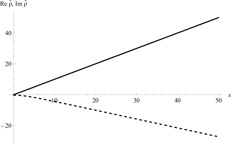
Figure 1: Numerical results of $\tilde{\rho}(x)$ with $m=1,g=0.1,x\in\left[0,50\right]$. $\mathrm{Re}\tilde{\rho}(x)$ and $\mathrm{Im}\tilde{\rho}(x)$ are represented by solid and dashed lines, respectively.

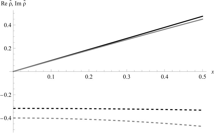
Figure 2: $x\in\left[0,0.5\right]$ region of Fig. 2, with perturbative results of $\mathrm{Re}\tilde{\rho}(x)$ and $\mathrm{Im}\tilde{\rho}(x)$ in gray solid and dashed lines.

Having established the existence of the $\tilde{\rho}$ tranformation, we turn to the $\eta$ transformation. A remarkable feature of the $\eta$ transformation in (11) is that the transformed action can be quadratic and thus has no interaction, and here we examine this special case. The $\eta$ transformation is solved from the following equation

$$\int_{C}d\phi\eta^{\prime}(\phi)\exp\left(-\frac{1}{2}m^{2}\eta(\phi)^{2}-ig\eta(\phi)^{3}\right)=\int_{\mathbbm{R}}d\phi\exp\left(-\frac{1}{2}m^{2}\phi^{2}-\Delta E_{0}\right).$$ (28)

Taking $C$ to be the constant phase contour (24) again, we can immediately write down the equation satisfied by $\eta(x)\equiv\eta(\phi_{C}(x))$ as follows,

$$\eta^{\prime}(x)\exp\left(-\frac{1}{2}m^{2}\eta(x)^{2}-ig\eta(x)^{3}\right)=\exp\left(-\frac{1}{2}m^{2}x^{2}-\Delta E_{0}\right),$$ (29)

$$\frac{1}{2}m^{2}\eta(x)^{2}+ig\eta(x)^{3}\rightarrow\frac{1}{2}m^{2}x^{2}\mbox{ when }|x|\rightarrow\infty,$$

where the boundary condition simply states $\eta^{\prime}(x)$ is subleading which is reasonable beacuse we expect the transformed contour $\eta(x)$ varies relatively slowly in large $x$, and $\Delta E_{0}$ can be decided by the $\mathcal{PT}$ symmety of $\eta(x)$ which requires $\eta^{*}(x)=-\eta(-x)$. Numerical result of $\eta(x)$ is shown in Fig. 4 and Fig. 4. Coefficients in (11) that transforms $i\phi^{3}$ to a free theory is $c_{1}=-1,c_{2}=-5/2,c_{3}=-2,c_{4}=-13/2,c_{5}=-5$, and corresponding $0$-dimensional perturbative results of $\eta(x)$ is thus

$$\eta(x)=\left.\phi-i\frac{g}{m^{2}}\phi^{2}-\frac{5}{2}\frac{g^{2}}{m^{4}}\phi^{3}-2i\frac{g}{m^{4}}-\frac{19}{2}\frac{g^{2}}{m^{6}}\phi\right|_{\phi=\phi_{C}(x)},$$ (30)

which is compared with numerical results in Fig. 4, and the difference between numerical and perturbative results is of higher order. (17) also predicts $\Delta E_{0}=(15g^{2})/(2m^{6})=0.075$ in the numerical setting, which gives leading contribution comparing to the numerical result $0.053405$.

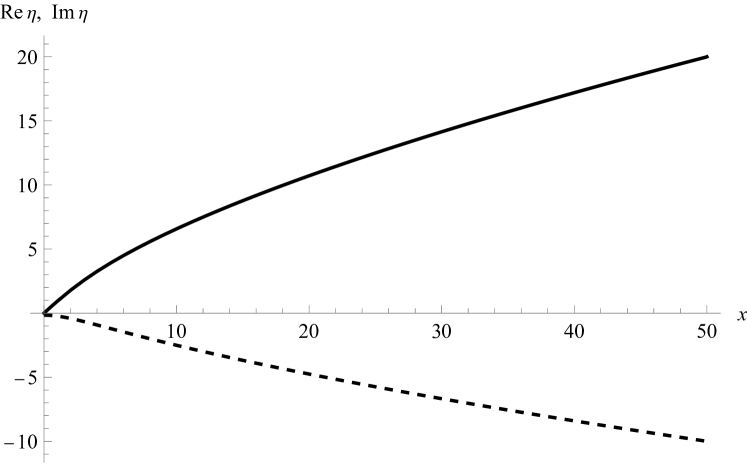
Figure 3: Numerical results of $\eta(x)$ with $m=1,g=0.1,x\in\left[0,50\right]$. $\Delta E_{0}$ is found to be $0.053405$. $\mathrm{Re}\eta(x)$ and $\mathrm{Im}\eta(x)$ are represented by solid and dashed lines, respectively.

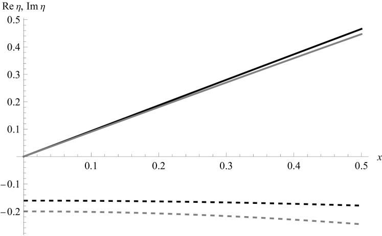
Figure 4: $x\in\left[0,0.5\right]$ region of Fig. 4, with perturbative results of $\mathrm{Re}\eta(x)$ and $\mathrm{Im}\eta(x)$ in gray solid and dashed lines.

Although weird, the transformation from $i\phi^{3}$ model to a quadratic model does exist, at least in $0$-dimension. And we futher show Hermitian non-quadratic actions can also be transformed to quadratic actions in $0$-dimension, by explicitly solving the following equation numerically for $V(x)=\lambda x^{4},\lambda x^{6}$,

$$\xi^{\prime}(x)\exp\left(-\frac{1}{2}m^{2}\xi(x)^{2}-V(\xi(x))\right)=\exp\left(-\frac{1}{2}m^{2}x^{2}-\Delta E_{0}\right),$$ (31)

$$\frac{1}{2}m^{2}\xi(x)^{2}-V(\xi(x))\rightarrow\frac{1}{2}m^{2}x^{2}\mbox{ when }|x|\rightarrow\infty,$$

where $\xi(x)$ is the corresponding tranformation. And $\Delta E_{0}$ can still be decided by the remaing $\mathcal{PT}$ symmety of $\xi(x)$ which requires $\xi(x)=-\xi(-x)$. Numerical results are shown in Fig. 6 and Fig. 6.

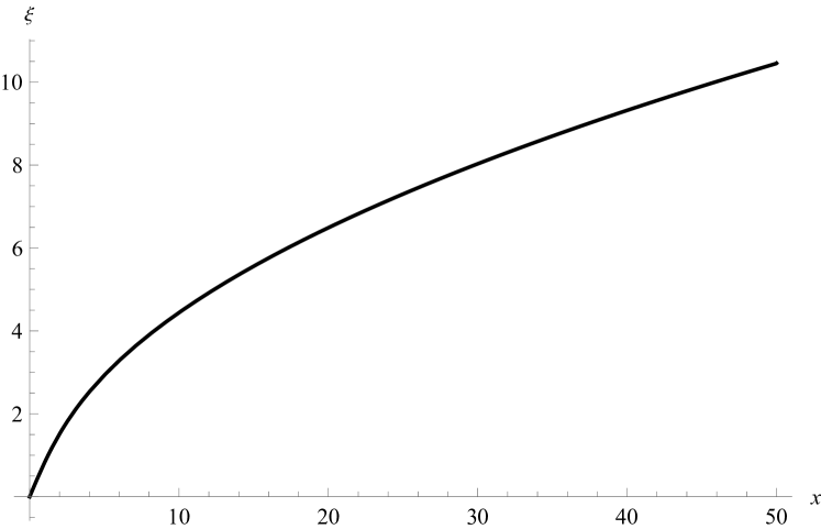
Figure 5: Numerical results of $\xi(x)$ with $m=1,V(x)=0.1x^{4},x\in\left[0,50\right]$. $\Delta E_{0}$ is found to be $0.153608$.

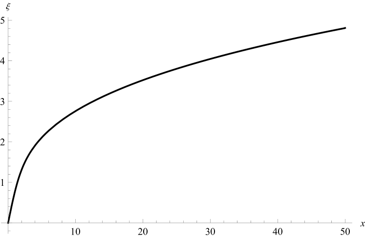
Figure 6: Numerical results of $\xi(x)$ with $m=1,V(x)=0.1x^{6},x\in\left[0,50\right]$. $\Delta E_{0}$ is found to be $0.208520$.

7 Conclusions

We have reformulated the $\mathcal{C}$ and $\eta$ operators related by $\mathcal{C}=\mathcal{P}\eta^{\dagger}\eta$, which are keys to calculate physical quantities in the $\mathcal{PT}$-symmetric $i\phi^{3}$ model, as manifestly 4-dimensional invariant transformations of field variables in path integral formalism. It is found that the transformation $\eta(\phi)$ as in (11) is not unique and transforms $i\phi^{3}$ to infinite Hermitian theories as shown by (17). No obvious arguments can be made to constrain parameters in the transformation. The existence of any physical meaning of perturbative $\mathcal{PT}$-symmetric models such as $i\phi^{3}$ model is thus a severe problem that prevents $\mathcal{PT}$-symmetric theories to be used in realistic model building.

To find the way out, we review possible deficiencies in this work. First, the convergence of perturbation series such as (10) and (11) is not guaranteed in $4$-dimension, and non-perturbative corrections may be of great importance. Second, we assume the contour of transformed fields can be deformed back to real axis, which is to say transformations proposed in this paper do not alter the Stokes sectors where the fields live thus lead to the same functional integralBender et al. (2019), and non-perturbative arguments in $4$-dimension are also needed to show this is indeed the case. Finally, we calculate only to the second order in the $i\phi^{3}$ model and higher-order results may be nontrivial and put constraints on $\eta(\phi)$. However, higher-order calculation is much more complicated and will be studied in future works. But at least, we have shown $0$-dimensional $i\phi^{3}$ model behaves well in the sense that transformations representing $C$ and $\eta$ operators do exist numerically and match perturbative expansions in small-coupling and small-field regions, which should give a primary confirmation of our proposal, noting that coefficients of those transformations are independent of dimension.

Moreover, in Xian et al. (2023) the global $U(1)$ parameter from a gauge theory was promoted to a complex number thus resulting $\mathcal{PT}$-symmetric Hamiltonians, and the arbitrariness of the $\eta$ operator is compensated by the gauge invariance of the theory. This suggests finding hidden symmetries in $\mathcal{PT}$-symmetric theories to reduce the large degrees of freedom of the $\eta$ operator. Optimistically, if the choice can be made to select the unique transformation that carries $i\phi^{3}$ to its Hermitian counterpart, the representation of the transformation in path integral formalism has another advantage comparing to canonical formalism besides the manifest 4-dimensional invariance, which is the manifest compatability with causality. After Wick-rotating to Minkowski space, the Euclidean propagator $D(x-y)=\int\frac{d^{4}p}{(2\pi)^{4}}\frac{e^{ip\cdot(x-y)}}{p^{2}+m^{2}}$ is simply substituted by the Feynman propagator $D_{F}(x-y)=\int\frac{d^{4}p}{(2\pi^{4})}\frac{ie^{-ip\cdot(x-y)}}{p^{2}-m^{2}+i0_{+}}$, and the causality violation in canonical formalism owing to the presence of non-Feynman propagator described in Novikov (2019) can be saved immediately.

References

- Bender and Boettcher (1998) Bender, C., Boettcher, S., 1998. Real spectra in non-hermitian hamiltonians having pt symmetry. Phys. Rev. Lett. 80, 5243–5246. doi:10.1103/PhysRevLett.80.5243.
- Bender (2007) Bender, C.M., 2007. Making sense of non-hermitian hamiltonians. Rep. Prog. Phys. 70, 947. doi:10.1088/0034-4885/70/6/R03.
- Bender (2011) Bender, C.M., 2011. Pt‐symmetric quantum field theory. AIP Conference Proceedings 1389, 642–645. doi:10.1063/1.3636813.
- Bender et al. (2002a) Bender, C.M., Berry, M.V., Mandilara, A., 2002a. Generalized pt symmetry and real spectra. J. Phys. A: Math. Gen. 35, L467. doi:10.1088/0305-4470/35/31/101.
- Bender et al. (2012) Bender, C.M., Branchina, V., Messina, E., 2012. Ordinary versus -symmetric quantum field theory. Phys. Rev. D 85, 085001. doi:10.1103/PhysRevD.85.085001.
- Bender et al. (2013) Bender, C.M., Branchina, V., Messina, E., 2013. Critical behavior of the -symmetric quantum field theory. Phys. Rev. D 87, 085029. doi:10.1103/PhysRevD.87.085029.
- Bender et al. (2005) Bender, C.M., Brandt, S.F., Chen, J.H., Wang, Q., 2005. The operator in -symmetric quantum field theory transforms as a lorentz scalar. Phys. Rev. D 71, 065010. doi:10.1103/PhysRevD.71.065010.
- Bender et al. (2002b) Bender, C.M., Brody, D.C., Jones, H.F., 2002b. Complex extension of quantum mechanics. Phys. Rev. Lett. 89, 270401. doi:10.1103/PhysRevLett.89.270401.
- Bender et al. (2004a) Bender, C.M., Brody, D.C., Jones, H.F., 2004a. Extension of -symmetric quantum mechanics to quantum field theory with cubic interaction. Phys. Rev. D 70, 025001. doi:10.1103/PhysRevD.70.025001.
- Bender et al. (2004b) Bender, C.M., Brody, D.C., Jones, H.F., 2004b. Scalar quantum field theory with a complex cubic interaction. Phys. Rev. Lett. 93, 251601. doi:10.1103/PhysRevLett.93.251601.
- Bender et al. (2019) Bender, C.M., Dorey, P.E., Dunning, C., et al., 2019. PT Symmetry: In Quantum and Classical Physics. WORLD SCIENTIFIC (EUROPE). doi:10.1142/q0178.
- Bender and Kuzhel (2012) Bender, C.M., Kuzhel, S., 2012. Unbounded -symmetries and their nonuniqueness. J. Phys. A: Math. Gen. 45, 444005. doi:10.1088/1751-8113/45/44/444005.
- Bender et al. (2003) Bender, C.M., Meisinger, P.N., Wang, Q., 2003. Calculation of the hidden symmetry operator in -symmetric quantum mechanics. J. Phys. A: Math. Gen. 36, 1973. URL: https://dx.doi.org/10.1088/0305-4470/36/7/312, doi:10.1088/0305-4470/36/7/312.
- Degrassi et al. (2012) Degrassi, G., Di Vita, S., Elias-Miro, J., et al., 2012. Higgs mass and vacuum stability in the standard model at nnlo. JHEP 08. doi:10.1007/JHEP08(2012)098.
- Dorey et al. (2001) Dorey, P., Dunning, C., Tateo, R., 2001. Spectral equivalences, bethe ansatz equations, and reality properties in -symmetric quantum mechanics. J. Phys. A: Math. Gen. 34, 5679. doi:10.1088/0305-4470/34/28/305.
- Dwivedi and Mandal (2021) Dwivedi, A., Mandal, B.P., 2021. Higher loop function for non-hermitian pt symmetric theory. Ann. Phys. 425, 168382. doi:https://doi.org/10.1016/j.aop.2020.168382.
- Fisher (1978) Fisher, M.E., 1978. Yang-lee edge singularity and field theory. Phys. Rev. Lett. 40, 1610–1613. URL: https://link.aps.org/doi/10.1103/PhysRevLett.40.1610, doi:10.1103/PhysRevLett.40.1610.
- Fujikawa (1980) Fujikawa, K., 1980. Comment on chiral and conformal anomalies. Phys. Rev. Lett. 44, 1733–1736. doi:10.1103/PhysRevLett.44.1733.
- Jones and Rivers (2007) Jones, H.F., Rivers, R.J., 2007. Disappearing operator. Phys. Rev. D 75, 025023. doi:10.1103/PhysRevD.75.025023.
- Mostafazadeh (2002a) Mostafazadeh, A., 2002a. Pseudo-hermiticity versus pt-symmetry. ii. a complete characterization of non-hermitian hamiltonians with a real spectrum. J. Math. Phys. 43, 2814–2816. doi:10.1063/1.1461427.
- Mostafazadeh (2002b) Mostafazadeh, A., 2002b. Pseudo-hermiticity versus pt-symmetry iii: Equivalence of pseudo-hermiticity and the presence of antilinear symmetries. J. Math. Phys. 43, 3944–3951. doi:10.1063/1.1489072.
- Mostafazadeh (2002c) Mostafazadeh, A., 2002c. Pseudo-hermiticity versus pt symmetry: The necessary condition for the reality of the spectrum of a non-hermitian hamiltonian. J. Math. Phys. 43, 205–214. doi:10.1063/1.1418246.
- Mostafazadeh (2003) Mostafazadeh, A., 2003. Exact pt-symmetry is equivalent to hermiticity. J. Phys. A: Math. Gen. 36, 7081. doi:10.1088/0305-4470/36/25/312.
- Novikov (2019) Novikov, O.O., 2019. Scattering in pseudo-hermitian quantum field theory and causality violation. Phys. Rev. D 99, 065008. doi:10.1103/PhysRevD.99.065008.
- Shalaby (2017) Shalaby, A.M., 2017. Vacuum structure and -symmetry breaking of the non-hermetian () theory. Phys. Rev. D 96, 025015. doi:10.1103/PhysRevD.96.025015.
- Shalaby (2019) Shalaby, A.M., 2019. Effective action study of the -symmetric theory and the yang–lee edge singularity. Int. J. Mod. Phys. A 34, 1950090. doi:10.1142/S0217751X19500908.
- Shalaby (2020) Shalaby, A.M., 2020. Extrapolating the precision of the hypergeometric resummation to strong couplings with application to the -symmetric field theory. Int. J. Mod. Phys. A 35, 2050041. doi:10.1142/S0217751X20500414.
- Weinberg (1995) Weinberg, S., 1995. The Quantum Theory of Fields Vol. 1: Foundations. Cambridge University Press.
- Xian et al. (2023) Xian, Z.Y., Fernández, D.R., Chen, Z., et al., 2023. Electric conductivity in non-hermitian holography. arXiv:2304.11183.