The LOFAR Two-metre Sky Survey: Deep Fields Data Release 1.
V. Survey description, source classifications and host galaxy properties

Abstract

Source classifications, stellar masses and star formation rates are presented for $\approx$80,000 radio sources from the first data release of the Low Frequency Array Two-metre Sky Survey (LoTSS) Deep Fields, which represents the widest deep radio survey ever undertaken. Using deep multi-wavelength data spanning from the ultraviolet to the far-infrared, spectral energy distribution (SED) fitting is carried out for all of the LoTSS-Deep host galaxies using four different SED codes, two of which include modelling of the contributions from an active galactic nucleus (AGN). Comparing the results of the four codes, galaxies that host a radiative AGN are identified, and an optimised consensus estimate of the stellar mass and star-formation rate for each galaxy is derived. Those galaxies with an excess of radio emission over that expected from star formation are then identified, and the LoTSS-Deep sources are divided into four classes: star-forming galaxies, radio-quiet AGN, and radio-loud high-excitation and low-excitation AGN. Ninety-five per cent of the sources can be reliably classified, of which more than two-thirds are star-forming galaxies, ranging from normal galaxies in the nearby Universe to highly-starbursting systems at $z>4$. Star-forming galaxies become the dominant population below 150-MHz flux densities of $\approx$1 mJy, accounting for 90 per cent of sources at $S_{\rm 150MHz}\sim 100\mu$Jy. Radio-quiet AGN comprise $\approx$10 per cent of the overall population. Results are compared against the predictions of the SKADS and T-RECS radio sky simulations, and improvements to the simulations are suggested.

1 Introduction

Understanding the formation and evolution of galaxies requires a detailed knowledge of the baryonic processes that both drive and quench the process of star formation within galaxies across cosmic time. In this regard, the faint radio sky provides one of the most important windows on the Universe, as it offers a direct view onto three critical (and overlapping) populations of objects: star-forming galaxies, ‘radio-quiet’ active galactic nuclei (AGN), and low luminosity radio galaxies (e.g. Padovani, 2016).

Arguably the most important observational test for any model of galaxy formation is measurements of the evolution of the cosmic star-formation rate density across cosmic time, and the distribution of that star formation amongst the galaxy population at each redshift, as a function of stellar mass, galaxy morphology, environment, and other properties. These crucial measurements require large, unbiased samples of star-forming galaxies over a wide range of redshifts. Much progress has been made in understanding the star-forming galaxy population, at least out to cosmic noon at $z\sim 2$, using a variety of star-formation indicators (e.g. Madau & Dickinson, 2014). The primary uncertainty is the effect of dust: by cosmic noon, around 85 per cent of the total star-formation rate (SFR) density of the Universe is dust-enshrouded (e.g. Dunlop et al., 2017), and a sub-millimetre (sub-mm) or far-infrared (far-IR) view of the Universe paints a very different picture of galaxy properties to that of a population selected at optical (rest-frame ultraviolet) wavelengths (e.g. Cochrane et al., 2021). Current far-IR surveys are limited by sensitivity to the more extreme systems, where contamination of the far-IR light by AGN emission is also a concern (e.g. Symeonidis & Page, 2021).

Radio emission provides a tool to observe the activity of galaxies in a manner that is independent of dust. For sources without AGN, the low-frequency radio emission arises primarily from recent supernova explosions of massive (young) stars (see reviews by Condon, 1992; Kennicutt, 1998), and thus directly traces the current star-formation rate (unless sufficiently low radio frequencies are reached such that free-free absorption becomes important; e.g. Schober et al., 2017). New generation radio interferometers offer sufficient sensitivity and field-of-view to survey large samples of star-forming galaxies out to high redshifts. Crucially, they can also provide sufficient angular resolution that deep surveys are not generally affected by the source confusion that limits the capabilities of surveys with sub-mm and far-IR telescopes such as the Herschel Space Observatory, for which the vast majority of sources in deep surveys are blends (e.g. Oliver et al., 2012; Scudder et al., 2016).

Star formation within massive galaxies is widely believed to be regulated in some manner by AGN, due to the large outflows of energy associated with the growth of supermassive black holes. AGN activity occurs in two fundamental modes (e.g. see reviews by Heckman & Best, 2014; Hardcastle & Croston, 2020). At high accretion rates, accretion of material on to a black hole is understood to occur through a ‘standard’ geometrically-thin, optically-thick accretion disk (Shakura & Sunyaev, 1973), in which around 10 per cent of the rest-mass energy of the accreting material is emitted in the form of radiation (‘radiative’ or ‘quasar-like’ AGN). These AGN can drive outflowing winds through thermal or radiation pressure (e.g. Fabian, 2012, and references therein), which may have a substantial effect on the evolution of the host galaxy. Radiatively-efficient AGN sometimes possess powerful twin radio jets (‘radio-loud’ quasars or their edge-on counterparts, the ‘high-excitation radio galaxies’; HERGs), and many recent works also suggest that even those that do not (‘radio-quiet’ AGN) frequently (or maybe even always) possess weak radio jets (Jarvis et al., 2019; Gürkan et al., 2019; Macfarlane et al., 2021; Morabito et al., 2022, and references therein). These AGN are detectable in deep radio surveys, either due to the weak radio jets or due to the star formation that can accompany the AGN activity.

At lower accretion rates, typically below about 1 per cent of the Eddington accretion rate, the nature of the accretion flow on to a supermassive black hole is believed to change: the accretion flow is thought to become geometrically thick and radiatively inefficient (Narayan & Yi, 1994, 1995). A characteristic feature of these advection-dominated or radiatively-inefficient accretion flows is that most of the energy that they release is in the form of two-sided radio jets (‘jet-mode’ AGN; also referred to as ‘low-excitation radio galaxies’). These jet-mode AGN dominate the radio sky at intermediate flux densities (above a few mJy), and the radio waveband is by far the most efficient means of identifying these sources. Jet-mode AGN have been very well-studied in the nearby Universe (e.g. Best & Heckman, 2012), where it is now widely accepted that they play a critical role in the evolution of massive galaxies and clusters, providing an energy input that counter-balances the radiative cooling losses of the surrounding hot gas and thus preventing that gas from cooling and forming stars (see reviews by McNamara & Nulsen, 2007; Fabian, 2012; Kormendy & Ho, 2013; Heckman & Best, 2014; Hardcastle & Croston, 2020, and references therein). Deeper radio surveys, probing the faint radio sky, enable these low-luminosity AGN to be detected and studied to higher redshifts (Best et al., 2014; Pracy et al., 2016; Williams et al., 2018; Whittam et al., 2022), and hence their role in the evolution of massive galaxies to be determined across cosmic time.

Deep radio surveys can therefore offer a unique insight into many aspects of the galaxy and AGN population. However, to extract the maximum science from deep radio surveys, it is essential that they are carried out in regions of the sky which are extremely well-studied at other wavelengths across the electromagnetic spectrum. The ancillary data are required to identify the radio source host galaxies, to estimate their redshifts, to classify the nature of the radio emission (star formation vs radiatively-efficient AGN vs jet-mode AGN) and to determine the physical properties of the host galaxies (stellar mass, star-formation rate, environment, etc).

Until recently, the state-of-the-art in wide-area deep radio surveys was the VLA-COSMOS 3 GHz survey (Smolčić et al., 2017a), which used the Very Large Array (VLA) to cover 2 deg² of the Cosmic Evolution Survey (COSMOS) field, arguably the best-studied degree-scale extragalactic field in the sky. Smolčić et al. (2017b) investigated the multi-wavelength counterparts of the $\approx$10,000 radio sources detected, and provided classifications, which then allowed several further investigations of the radio-AGN and star-forming populations (e.g. Smolčić et al., 2017c; Novak et al., 2017; Delvecchio et al., 2017; Delhaize et al., 2017). Nevertheless, even the VLA-COSMOS 3 GHz survey does not have sufficient sky area to cover all cosmic environments, and may therefore suffer from cosmic variance effects, as well as having limited source statistics at the highest redshifts. The on-going MeerKAT International GigaHertz Tiered Extragalactic Exploration (MIGHTEE) 1.4 GHz survey aims to extend sky coverage at this depth to 20 deg²; Heywood et al. (2022) provide an early release, with Whittam et al. (2022) deriving source classifications for 88 per cent of the $\approx 5,000$ sources with host galaxy identifications over 0.8 deg² in the COSMOS field.

The Low Frequency Array (LOFAR; van Haarlem et al., 2013) Two-metre Sky Survey (LoTSS) Deep Fields have a similar goal at lower frequency. The first data release (hereafter LoTSS-Deep DR1) was made public in April 2021: the radio data reach rms sensitivity levels $\approx 4$ times deeper than the wider all-northern-sky LoTSS survey (Shimwell et al., 2017, 2019, 2022), corresponding to approximately the same effective depth as the VLA-COSMOS 3 GHz survey (for a source with typical radio spectral index, $\alpha\approx 0.7$, where $S_{\nu}\propto\nu^{-\alpha}$) but over an order of magnitude larger sky area (Tasse et al., 2021; Sabater et al., 2021, hereafter Papers I and II respectively). An extensive optical and near-infrared cross-matching process has identified and provided detailed photometry for over 97 per cent of the $\approx$80,000 radio sources detected over the central regions of the target fields where the best ancillary data are available (a combined area of 25 deg²; Kondapally et al., 2021, Paper III). These data have been used to provide high-quality photometric redshifts (Duncan et al., 2021, Paper IV). In this paper, the 5th of the series, these data are combined with far-IR data to carry out detailed spectral energy distribution (SED) fits to the multi-wavelength photometry from ultraviolet (UV) to far-IR wavelengths, using several different SED fitting codes. Using the results of this analysis, the radio sources are classified into their different types, and key physical parameters of the host galaxies, such as their stellar masses and star-formation rates, are determined.

The layout of the paper is as follows. In Sec. 2 the LoTSS Deep Fields survey is described: this section outlines the choice of target fields, and places the first data release in to the context of the eventual full scope of the survey. Sec. 3 then describes the data that will be used in the paper and outlines the application of the SED fitting algorithms. Sec. 4 describes how the results are used to identify the (radiative-mode) AGN within the sample. The results of the different SED fitting algorithms are compared in Sec. 5, and used to define consensus measurements for the stellar mass and star-formation rate of each host galaxy. Combining this information with the radio data, Sec. 6 then describes the identification of radio-excess AGN. Sec. 7 summarises the final classifications of the objects in the sample, and investigates the dependence of these on radio flux density, luminosity, stellar mass and redshift. In Sec. 8 the results are compared against the predictions of the most widely-used radio sky simulations, and suggestions made for improvements to those simulations. Finally, conclusions are drawn in Sec. 9. The classifications derived are released in electronic form and are used for detailed science analysis in several further papers (Smith et al., 2021; Bonato et al., 2021; Kondapally et al., 2022; McCheyne et al., 2022; Mingo et al., 2022; Cochrane et al., 2023, and others).

Throughout the paper, cosmological parameters are taken to be $\Omega_{m}=0.3$, $\Omega_{\Lambda}=0.7$ and $H_{0}=70$ km s^-1 Mpc^-1, and the Chabrier (2003) initial mass function is adopted.

2 The LoTSS Deep Fields

2.1 LOFAR observations of the LoTSS Deep Fields

The International LOFAR Telescope (van Haarlem et al., 2013) is a remarkably powerful instrument for carrying out deep and wide radio surveys of the extragalactic sky, owing to its high sensitivity, high angular resolution (6 arcsec at 150 MHz when using only Dutch baselines, improving to 0.3 arcsec with the international stations included), and in particular its wide field-of-view. The primary beam full-width at half-maximum (FWHM) of the Dutch LOFAR stations is 3.8 degrees at 150 MHz, giving a field-of-view of more than 10 deg² in a single pointing. International stations have a larger collecting area and a correspondingly smaller beam: 2.5 deg FWHM; 4.8 deg² field-of-view. The LoTSS survey (Shimwell et al., 2017, 2019, 2022) is exploiting LOFAR’s capabilities by observing the entire northern sky, with a target rms depth of below 100$\mu$Jy beam^-1 at favourable declinations (the non-steerable nature of the LOFAR antennas means that sensitivity decreases at lower elevations). Nevertheless, LoTSS only scratches the surface of the depth that radio surveys with LOFAR are capable of reaching. LoTSS provides an excellent census of the radio-loud AGN population which dominates the bright and intermediate radio sky, but samples only the brighter end of the radio-quiet AGN and star-forming galaxy populations which become dominant as the LoTSS flux density limit is approached.

The LoTSS Deep Fields provide a complementary deeper survey, aiming to reach a noise level of 10-15 $\mu$Jy beam^-1 over a sky area of at least 30 deg². LoTSS-Deep is designed to have the sensitivity to detect Milky-Way-like galaxies out to $z>1$, and galaxies with star-formation rates of 100$M_{\odot}$ yr^-1 to beyond $z=5$ (e.g. Smith et al., 2016), as well as being able to detect typical radio-quiet quasars right out to redshift 6 (Gloudemans et al., 2021). The sky area makes it possible to: (i) sample the full range of environments at high redshifts – for example, it is expected to include 10 rich proto-clusters at $z>2$; (ii) include statistically meaningful samples of rarer objects (such as $z>5$ starbursts); (iii) build large enough samples of AGN and star-forming galaxies (over 100,000 of each expected to be detected) to allow simultaneous division by multiple key properties, such as luminosity, redshift, stellar mass and environment.

LoTSS-Deep is being achieved through repeated 8-hr LOFAR observations of the regions of the northern sky with the highest quality degree-scale multi-wavelength data. The four target fields are the European Large Area ISO Survey Northern Field 1 (ELAIS-N1; Oliver et al., 2000), the Boötes field (Jannuzi & Dey, 1999), the Lockman Hole (Lockman et al., 1986) and the North Ecliptic Pole (NEP); these are described in more detail in Section 2.3.

Table 1: Status of observations and imaging in LOFAR Deep Fields, including the data released in the LoTSS Deep Fields 1st data release (LoTSS-Deep DR1). The area of best ancillary data is defined in Paper III. Quoted rms noise levels are those at the centre of the field. The marginally lower sensitivity in Boötes compared to the other fields is due to its lower declination, and hence lower average elevation during the observations. The ‘number of sources in DR1 full area’ quoted is over the full catalogues presented in Paper I and Paper II, out to the 30 per cent power point of the primary beam (ie. over $\sim 25$ deg² in each field).

Field	Coordinates	Area of best	Obs. time	central rms	No sources	No sources	Final awarded	Target
	(J2000)	ancillary data	in DR1	noise in DR1	full DR1	best ancillary	integration	rms depth
		[deg2]	[hrs]	[$\mu$Jy/beam]	area	data area	time [hrs]	[$\mu$Jy/beam]
ELAIS-N1	16 11 00   +54 57 00	6.74	164	19	84,862	31,610	500	11
Boötes	14 32 00   +34 30 00	8.63	80	32	36,767	31,162	312	16
Lockman Hole	10 47 00   +58 05 00	10.28	112	22	50,112	19,179	352	13
NEP	17 58 00   +66 00 00	10.0	–	–	–	–	400	13

Table 1 outlines the anticipated final depths of each field based on awarded observing time. Scaling by depth and area from radio source counts in shallower LoTSS-Deep observations, the final LoTSS Deep Fields are expected to detect more than 250,000 radio sources within the central 35 deg², overlapping the best multi-wavelength data. Figure 1 compares the sensitivity, field-of-view, and angular resolution of the LoTSS Deep Fields to other completed and on-going radio surveys. The final LoTSS Deep Fields dataset will be unrivalled in its combination of depth and area. The inclusion of the international stations will also provide an angular resolution which is unmatched by any competitor survey: indeed, at low frequencies, the LoTSS Deep Fields with international baselines will remain unique even in the era of the Square Kilometre Array (SKA).

In order to account for the smaller primary beam of the international stations, from LOFAR Observing Cycle 14 onwards the pointing positions for the LoTSS-Deep observations of the Lockman Hole, Boötes and NEP fields have been dithered around a small mosaic. The mosaics have been designed to ensure good coverage of the sky area with the best-quality multi-wavelength data, within the primary beam of the international stations, while keeping offsets small enough so that there is negligible loss of sensitivity over this region when imaging with only Dutch stations.

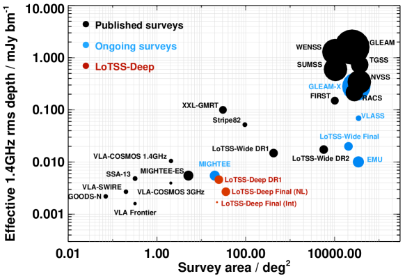
Figure 1: The survey depth, area and angular resolution of the LoTSS Deep Fields compared to other existing and on-going radio surveys. All survey depths are converted to a 1.4 GHz equivalent rms depth using a spectral index of $\alpha=0.7$. The black points show published surveys, and the blue points show on-going surveys. The LoTSS Deep Fields are highlighted in red. The size of each symbol indicates the angular resolution of the survey, with the symbol area proportional to the beam FWHM. For the LoTSS Deep Fields final release, the larger symbol indicates the result of including just the Dutch baselines, while the smaller symbol shows what should be achievable after including the international stations (improved angular resolution, additional depth due to the extra collecting area, but smaller areal coverage due to the smaller primary beam of the international stations). Descriptions of the surveys included on the plot (listed from high to low effective rms depth) can be found in the following references: GLEAM (Wayth et al., 2015); WENSS (Rengelink et al., 1997); TGSS (Intema et al., 2017); SUMSS (Mauch et al., 2003); NVSS (Condon et al., 1998); GLEAM-X (Hurley-Walker et al., 2022); RACS (Hale et al., 2021); FIRST (Becker et al., 1995); XXL-GMRT (Smolčić et al., 2018); VLASS (Lacy et al., 2020); Stripe82 (Hodge et al., 2011); LoTSS-Wide (Shimwell et al., 2019); VLA-COSMOS 1.4 GHz (Schinnerer et al., 2007); EMU (Norris et al., 2011); MIGHTEE (including Early Science – ES; Heywood et al., 2022) SSA-13 (Fomalont et al., 2006); VLA-COSMOS 3 GHz (Smolčić et al., 2017a); VLA-SWIRE (Owen & Morrison, 2008); GOODS-N (Owen, 2018); VLA Frontier (Heywood et al., 2021).

2.2 LoTSS-Deep DR1

This paper considers the radio source catalogues from the first LoTSS Deep Fields data release. LoTSS-Deep DR1 released the reduced LOFAR images and catalogues constructed from data taken before October 2018 (; ), along with the optical/IR catalogues and host galaxy identifications (Paper III) and photometric redshifts (Paper IV). These LoTSS-Deep DR1 LOFAR observations focused on the ELAIS-N1, Boötes and Lockman Hole fields, due to the earlier availability of the multi-wavelength data in those fields. The LoTSS-Deep DR1 LOFAR images included only the data from the Dutch LOFAR stations, not the international stations, due to the additional complications associated with calibrating the long baselines and the associated computing requirements (see e.g. Morabito et al., 2022; Sweijen et al., 2022, for a description of recent advances towards a pipeline for international stations). The data allow an angular resolution of 6 arcsec to be achieved: higher angular resolution images will be produced in later data releases.

As shown in Table 1, the images in LoTSS-Deep DR1 already reach an rms noise level below 20$\mu$Jy beam^-1 at 150 MHz at the centre of the deepest field (ELAIS-N1), away from bright sources. Sensitivity decreases with primary beam attenuation towards the outer regions of the field; dynamic range effects are also present around bright sources but only a few percent of the image suffers from significantly increased noise levels due to these calibration issues (; ). Over 170,000 sources are catalogued, with peak flux densities above 5 times the local rms noise, across the full radio area of the three fields; as with all radio catalogues, imcompleteness effects come in as the flux limit is approached (see Kondapally et al., 2022; Cochrane et al., 2023, for an analysis of the completeness for AGN and SFGs, respectively). More than 80,000 sources are catalogued in the central regions with the best multi-wavelength data (Paper III). As can be seen in Figure 1, LoTSS-Deep DR1 broadly matches the depth of the VLA-COSMOS 3GHz survey but over an order of magnitude larger sky area; similarly it matches the recent MeerKAT MIGHTEE Early Release (Heywood et al., 2022) in rms depth (the latter being limited by source confusion owing to its lower angular resolution), but again over larger area.

2.3 Multi-wavelength data in the LoTSS Deep Fields

ELAIS-N1, Boötes, Lockman Hole and NEP are the premier large-area northern extragalactic fields, with vast amounts of telescope time across the electromagnetic spectrum invested in observing these fields over the last two decades. Imaging at optical and near-IR wavelengths reaches 3-4 magnitudes deeper than typical all-sky surveys, allowing host galaxy identifications for over 97 per cent of the hosts of the radio sources in LoTSS-Deep DR1 (Paper III) compared to just 73 per cent using all-sky surveys in the LoTSS DR1 release (Williams et al., 2019). Other datasets, such as deep Herschel and Spitzer data in these fields, are irreplaceable, and add greatly to the scientific potential: Herschel data are a key tool to constrain obscured star-formation rates, while the mid-IR wavelengths covered by Spitzer contain the diagnostic emission from the AGN torus. This range of complementary data makes these excellent fields to study not only the high-redshift AGN and luminous star-forming galaxies detected by LOFAR, but also to understand how this activity sits within the wider cosmological context of the underlying galaxy population.

As well as their combined benefit of sky area and sample size, each of the four LoTSS Deep Fields possesses unique characteristics or datasets which further enhance its specific scientific potential, whilst complementing each other. The specific data available in each field are summarised here; a more complete description of the available data in the ELAIS-N1, Lockman Hole and Boötes fields (but not NEP, as it was not included in the LoTSS-Deep DR1) can be found in Paper III, which also provides the coverage maps of each survey and the resulting catalogues.

2.3.1 ELAIS-N1

ELAIS-N1 has an ideal declination (+55 deg) for LOFAR observations, and is also a target field for LOFAR’s Epoch of Reionisation studies (Jelić et al., 2014), providing a combined motivation for the observations. ELAIS-N1 benefits from some of the deepest wide-field optical, near-IR and mid-IR imaging. It is one of the Medium Deep Fields from the Panoramic Survey Telescope and Rapid Response Sysytem (Pan-STARRS-1) survey (Chambers et al., 2016), covering a 7 deg² field-of-view in the optical $g$,$r$,$i$,$z$,$y$ bands. It is a Hyper-Suprime-Cam Subaru Strategic Program (HSC-SSP; Aihara et al., 2018) optical deep field, with deep observations in $g$,$r$,$i$,$z$,$y$ and the narrow-band NB921 over 7.7 deg². $u$-band data over this full field are available from the Spitzer Adaptation of the Red-sequence Cluster Survey (SpARCS; Muzzin et al., 2009), and UV data were taken by the Galaxy Evolution Explorer (GALEX) space telescope as part of the Deep Imaging Survey (Martin et al., 2005). ELAIS-N1 also possesses deep near-IR imaging in $J$ and $K$ bands from the United Kingdom Infrared Deep Sky Survey (UKIDSS; Lawrence et al., 2007) Deep Extragalactic Survey (DXS), covering nearly 9 deg².

Mid-infrared data were acquired by Spitzer through both the Spitzer Wide-area Infra-Red Extragalactic survey (SWIRE; Lonsdale et al., 2003) in IRAC channels 1 to 4 (3.6–8.0$\mu$m) over $\sim 10$ deg² and the Spitzer Extragalactic Representative Volume Survey (SERVS; Mauduit et al., 2012), which is around a magnitude deeper at 3.6 and 4.5$\mu$m in the central 2.4 deg². Longer wavelength data in the field have been taken using both Spitzer (24$\mu$m data with the Multi-band Imaging Photometer for Spitzer; MIPS) and the Herschel Space Observatory, the latter as part of the Herschel Multi-tiered Extragalactic Survey (HerMES; Oliver et al., 2012), one of the deepest large-area Herschel surveys. HerMES observed ELAIS-N1 at 100$\mu$m, 160$\mu$m, 250$\mu$m, 350$\mu$m and 500$\mu$m.

2.3.2 Boötes

The Boötes field is the target of some of the deepest wide-field optical imaging, in the $B_{W}$, $R$ and $I$ filters from the NOAO Deep Wide Field Survey (Jannuzi & Dey, 1999), in the $z$-band from the zBoötes survey (Cool, 2007), and in the $U$ and $Y$ bands from the Large Binocular Telescope (Bian et al., 2013), all covering around 10 deg². The same sky region has been observed in the near-IR $J$, $H$ and $K$ bands (Gonzalez et al., 2010) and using Spitzer from 3.6 to 8.0$\mu$m as part of the Spitzer Deep Wide Field Survey (SDWFS; Ashby et al., 2009). Catalogues of galaxies in the Boötes field were generated by Brown et al. (2007); Brown et al. (2008). Boötes has also been observed by Herschel as part of HerMES, and by Spitzer-MIPS, adding far-infrared measurements to the dataset.

In addition to this, Boötes benefits from excellent wide-field X-ray coverage, including a deep Msec Chandra survey over the full 9.3 deg² field (Masini et al., 2020). The comparison between deep radio and deep X-ray observations opens many new scientific avenues, such as investigating the relationship between jet power and accretion rate in AGN, and determining the black hole accretion rates of star-forming galaxies to investigate the co-evolution of galaxies and black holes. Boötes also possesses a vastly higher number of spectroscopic redshifts than the other northern deep fields, largely due to the AGN and Galaxy Evolution Survey (AGES; Kochanek et al., 2012): these are also very valuable for training photometric redshifts for the radio source population (e.g. Paper IV, ).

2.3.3 Lockman Hole

Located (like ELAIS-N1) at an ideal declination for LOFAR (+58 deg), the Lockman Hole is one of the regions of sky with the lowest Galactic HI column density (Lockman et al., 1986), making it ideal for extragalactic studies, especially at IR wavelengths due to its low IR background. For this reason, the Lockman Hole has been the target of some of the widest deep coverage in the optical to mid-IR bands. Optical data in the Lockman Hole has been taken by SpARCS in $u$,$g$,$r$,$z$ over 13.3 deg², and by the Red Cluster Sequence Lensing Survey (RCSLenS; Hildebrandt et al., 2016) in $g$,$r$,$i$,$z$ over 16 deg² (albeit not contiguous). As with ELAIS-N1, UV data have been obtained by the GALEX Deep Imaging Survey, deep near-IR $J$ and $K$ band data are available as part of the UKIDSS-DXS survey (8 deg²), mid-IR data are available from both SWIRE (Channels 1–4 over 11 deg²) and SERVS (3.6 and 4.5 $\mu$m; 5.6 deg²) and far-IR data are available over the whole field from both Spitzer-MIPS imaging (24$\mu$m) and the Herschel HerMES project (100$\mu$m, 160$\mu$m, 250$\mu$m, 350$\mu$m and 500$\mu$m).

The Lockman Hole is arguably the best-studied of the deep fields at other radio frequencies (e.g. Mahony et al., 2016; Prandoni et al., 2018; Morganti et al., 2021). The multi-frequency radio data allow detailed investigations of radio spectral shapes, identifying peaked, remnant and re-started sources, and giving a unique insight into the physics and lifecycles of radio-loud AGN (e.g. Brienza et al., 2017; Jurlin et al., 2020).

2.3.4 North Ecliptic Pole

The North Ecliptic Pole is an interesting field due to its location in the continuous viewing zone (CVZ) of many space telescopes, including the JWST, the eROSITA X-ray mission and Euclid. Until very recently, the multi-wavelength data quality in the NEP was inferior to the other three LoTSS Deep Fields, but this is rapidly changing. The NEP is the location of the Euclid Deep Field North which will provide deep sub-arcsecond near-IR imaging to depths of $H=26$ over 10 deg² (and slightly shallower over a wider 20 deg² region). Such deep data will enable mass-complete samples to be defined down to $\sim 10^{10}M_{\odot}$ at $z=3$ and normal star-forming galaxies to be detected out to $z>6$. The combination of matched sub-arcsecond near-IR and radio continuum imaging (with LOFAR’s international baselines) offers a unique opportunity to study the structural evolution of galaxies, for example comparing the spatial distribution of star formation (probed by LOFAR) versus stellar mass (probed by Euclid) within galaxies, to cleanly distinguish between different growth scenarios (e.g. ‘inside-out’ or ‘outside-in’ growth) over large samples of massive galaxies with $z<1$.

Given these forthcoming datasets, a number of photometric surveys have been recently undertaken to provide matching observations at other wavelengths, including the Hawaii Two-0 survey (McPartland et al., 2023). Additionally, the Euclid/WFIRST Spitzer Legacy Survey has obtained mid-infrared imaging over the central 10 deg² of the field using Spitzer that is $\sim$0.8mag deeper than the SERVS data available in ELAIS-N1 and Lockman Hole.

As shown in Table 1, the NEP is not included in LoTSS-Deep DR1, and hence not included in the analysis of this paper, as the radio data were not available at the time of the optical cross-identification. An image from 72-hrs of data is now available and will be published by Bondi et al. (2023). Furthermore, as LOFAR observes two HBA pointings simultaneously, observations of the NEP field have included a parallel beam centred on the Abell 2255 cluster, which has also produced an ultra-deep low-frequency image of that field (Botteon et al., 2022).

3 Characterising the LoTSS-Deep host galaxies

3.1 Optical to mid-IR data

For the three fields presented in LoTSS-Deep DR1 (ELAIS-N1, Boötes, Lockman Hole), Paper III presented photometric catalogues from ultraviolet to far-infrared wavelengths. The reader is referred to that paper for a full description of the catalogues; here, a brief overview is provided.

For the ELAIS-N1 and Lockman Hole fields, data from UV through to mid-IR wavelengths were assembled and mosaicked on to a common pixel scale. Two combined $\chi^{2}$ signal-to-noise images were then constructed, one by combining the optical to near-IR bands, and the other from the Spitzer 3.6 and 4.5$\mu$m bands; these were treated separately due to the mis-match in angular resolution between the ground-based optical-to-near-IR and the Spitzer images. Forced aperture photometry was then performed across all bands using sources detected in each of these stacked images, and the two catalogues were merged to produce a single consistent photometric catalogue in each field. Aperture corrections were applied band-by-band based on curve-of-growth analysis for typical faint galaxies in order to provide total flux and total magnitude measurements. The photometry was corrected for galactic extinction based on the Milky Way E(B-V) extinction map of Schlegel et al. (1998) and the Milky Way dust extinction law of Fitzpatrick (1999). Uncertainties on the photometry were determined using the variations between a large number of apertures randomly placed around the fields.

For the Boötes field, forced aperture photometry catalogues already existed (Brown et al., 2007; Brown et al., 2008) using magnitude-limited samples selected in the I-band and the 4.5$\mu$m Spitzer band. In this case, these catalogues were used as the starting point, and were merged and corrected in a similar manner to ELAIS-N1 and Lockman Hole. In all three fields, the catalogues were then cleaned of low-significance detections (sources detected in the combined $\chi^{2}$ image but below 3$\sigma$ significance in each individual band) and cross-talk artefacts, and those sources in regions around bright stars where either the cataloguing or the photometry might be unreliable were flagged, as indicated by the flag_clean parameter. More details on all of these processes can be found in Paper III.

These photometric catalogues were then used as the basis for cross-matching with the LOFAR catalogues. Paper III outlines the selection of the studied area for which the highest-quality multi-wavelength data are available; sources within this region can be identified using the flag_overlap parameter. The cross-matching process also involved source association, such that the catalogued LOFAR sources were combined or deblended into true physical sources, where necessary. Within these defined areas, 81,951 physically distinct radio sources were catalogued over 25.65 deg² of sky across the three fields; optical or near-IR host galaxies were identified for over 97 per cent of these (Paper III), very much higher than the 73 per cent found for the wider LoTSS DR1 (Williams et al., 2019).

Photometric redshifts for all of the objects in the field have been presented in Paper IV. These were derived from the UV to mid-IR data by combining machine learning and template fitting approaches using a hierarchical Bayesian framework. This method is shown to provide photometric redshifts which are accurate for both galaxy populations (out to $z\approx 1.5$) and sources dominated by AGN emission (out to $z\approx 4$), which is important for the LOFAR sample. As part of the calibration of the photometric redshifts, small (typically <5 per cent) offsets in the zero-point magnitudes were found to improve the accuracy of the template-fit photometric redshifts. These offsets are discussed further in Section 3.3.

3.2 Far-infrared data

The addition of far-IR photometry is described by McCheyne et al. (2022), and the reader is referred to that paper for details. In summary, the far-IR fluxes were measured using XID+ (Hurley et al., 2017) which is a Bayesian tool to deblend the flux from the low resolution Herschel data into different potential host galaxies selected from optical/near-IR images. Fluxes were initially measured as part of the Herschel Extragalactic Legacy Project (HELP; Shirley et al., 2021). In HELP, an XID+ prior list of potential emitters at 24$\mu$m was derived by applying a number of cuts to the optical-IR galaxy catalogue in order to select the sources most likely to be bright at 24$\mu$m (those detected both at optical wavelengths and in the Spitzer 3.6-8.0$\mu$m bands), and this input list was used to deblend the 24$\mu$m data. Then, a second prior list was constructed from those sources with significant 24$\mu$m emission (above 20$\mu$Jy) and this was used to deblend the Herschel data. The posterior distributions for the fluxes derived from XID+ allow the uncertainties to be estimated.

For the LoTSS-Deep catalogue, a cross-match was first made between each LoTSS-Deep host galaxy position (or its LOFAR position if there was no host galaxy identification at optical-IR wavelengths) and the HELP catalogue. If a match was found then the HELP far-IR fluxes were assigned to the LOFAR source. If no match was found, then XID+ was re-run following the process above, but with the radio host galaxy position (or radio position in the case of no host galaxy identification) added to the prior list: this ensures that the assignment of zero flux is not simply due to the radio source having been incorrectly excluded from the prior list.

3.3 Final catalogues for spectral energy distribution fitting

In order to ensure consistency and reliability across the different spectral energy distribution (SED) fitting codes used in this paper, it was important to ensure that the input dataset was as robust as possible, and that all photometric errors were uniformly treated.

For each field, a catalogue was produced combining the (aperture-corrected and Galactic extinction corrected) fluxes from UV to mid-IR wavelengths with the far-IR fluxes determined by XID+. Next, the small zero-point magnitude corrections determined during the photometric redshift fitting were applied: these are tabulated in Appendix B of Paper IV. Specifically, the corrections derived using the extended Atlas library (referred to as ‘Brown’ in that paper) were applied; this template set was chosen because it extended out to the longest IRAC wavelength and also incorporated the full range of SED types expected within the LoTSS Deep Fields sample.

The photometry catalogue was then filtered to remove photometric measurements deemed to be seriously unreliable. These unreliable measurements were identified as those which were either 2.5 magnitudes lower, or 1 magnitude higher, than the value predicted by interpolating the two adjacent filter measurements. These limits were chosen, following Duncan et al. (2019), to avoid flagging any reasonable spectral emission or absorption features, or genuine breaks, while successfully identifying those measurements that are so discrepant that they could significantly influence the SED fitting. Around 1 per cent of the photometric measurements were identified in this way; these were flagged and not used in the subsequent fitting.

Finally, in order to consistently deal with any residual photometric errors due to zero-points, aperture corrections or extinction corrections, 10 per cent of the measured flux was added in quadrature to all flux uncertainties. The resultant SED input catalogues for each field are made available in electronic form through the LOFAR Surveys website (lofar-surveys.org).

3.4 Spectral Energy Distribution fitting

Many different codes exist for fitting SEDs to an array of photometric data points for galaxies and AGN. Each of these has their own advantages and disadvantages. Pacifici et al. (2023) recently carried out a detailed comparison of different codes, finding that they provide broad agreement in stellar masses, but with more discrepancies in the star formation rates and dust attenuations derived. In this paper, four different SED-fitting codes are adopted, and a comparison of the results between these is used both to derive consensus measurements for stellar masses and star-formation rates, and to assist with the classification of the radio source host galaxies.

The ‘Multi-wavelength Analysis of Galaxy Physical Properties’ (magphys; da Cunha et al., 2008) and ‘Bayesian Analysis of Galaxies for Physical Inference and Parameter EStimation’ (bagpipes; Carnall et al., 2018, 2019) codes each use energy balance approaches to fit photometric points from the UV through to far-IR and sub-mm wavebands. Energy balance implies that the amount of energy absorbed by dust at optical and UV wavelengths is forced to match that emitted (thermally) by the dust through the sub-mm and far-IR. The magphys and bagpipes codes are built on the same fundamental templates for single stellar populations (Bruzual & Charlot, 2003) but differ in their implementation, in particular with regard to the parameterisation of the star-formation histories of the galaxies, the assumed dust models, and the approach to model optimisation. For high signal-to-noise galaxies the two codes generally give broadly consistent results (see Sec. 5), which previous studies have generally shown to be accurate (e.g. Hayward & Smith, 2015). However, neither magphys nor bagpipes includes AGN emission in its model SEDs, nor do they account for AGN heating effects when determining energy balance, and therefore both can give poor fits and unreliable host galaxy parameters for galaxies with significant AGN emission.

‘Code Investigating GALaxy Emission’ (cigale; Burgarella et al., 2005; Noll et al., 2009; Boquien et al., 2019) is another broad-band SED-fitting code which uses energy conservation between the attenuated UV/optical emission and the re-emitted IR/sub-mm emission; cigale differs from magphys and bagpipes in that it incorporates AGN models which can account for the direct AGN light contributions and the infrared emission arising from AGN heating of the dust (more recent developments also allow for predictions of X-ray emission, cf. Yang et al., 2020). The inclusion of AGN models can give cigale a significant advantage over magphys and bagpipes when fitting the SEDs of galaxies that have a signficant AGN contribution, allowing both more robust estimation of host galaxy parameters, and a mechanism to identify and classify AGN within the sample. However, in order to allow the additional complications of AGN fitting, for equivalent (practical) run times cigale is not able to cover the parameter space of host galaxy properties as finely as magphys and bagpipes, leading to potentially less accurate characterisation of galaxies that do not host AGN.

All of the three codes discussed above adopt the principles of energy balance. However, if the distribution of ultraviolet light is spatially disconnected from the dust emission, as is often the case for very infrared luminous galaxies, then energy balance may not be valid; indeed, Buat et al. (2019) find for a sample of 17 well-studied dust-rich galaxies that SED-based UV-optical attenuation estimates account for less than half of the detected dust emission. This issue may be particularly pronounced in the presence of AGN, if the AGN models are not comprehensive enough to properly cover the parameter space of possible AGN SEDs. To mitigate these issues, the agnfitter code (Calistro Rivera et al., 2016) models the SED by independently fitting four emission components, with each independently normalised (albeit with a prior that the energy radiated in the infrared must be at least equal to the starlight energy absorbed by dust at optical/UV wavelengths): a big blue bump, a stellar population, hot dust emission from an AGN torus, and colder dust emission. agnfitter can provide superior fits for objects where energy balance breaks down, and also for objects with strong AGN components due to its superior modelling of the big blue bump. However, the lack of energy balance and the ability of the four components to vary independently can lead to aphysical solutions, or poorer constraints on the parameters of the stellar populations (although Gao et al. 2021 find broadly good agreement in measured stellar masses and SFRs between codes with and without energy balance, at least for hyperluminous infrared galaxies).

To maximise the advantages of the different techniques, the LoTSS Deep Field host galaxies were all modelled using each of magphys, bagpipes, cigale and agnfitter. Furthermore, for cigale, two different sets of AGN models were considered: those of Fritz et al. (2006) and those of Stalevski et al. (2012, 2016), the latter of which were recently incorporated into cigale by Yang et al. (2020). The following subsections provide details of the fitting methodology in each case.

For all SED fitting, the redshift of the source is fixed at the spectroscopic redshift, $z_{\rm{spec}}$, for the minority of sources for which this exists (1602, 4039 and 1466 sources in ELAIS-N1, Boötes and Lockman, respectively). For the other sources, the redshift is fixed at the median of the first photometric redshift solution, $z_{\rm 1,median}$. Photometric redshift errors may introduce errors on the inferred parameters, but for most sources these are anticipated to be small since the photometric redshifts are very accurate, with a median scatter of $\Delta z/(1+z)\mathrel{\hbox to0.0pt{\lower 3.0pt\hbox{$\mathchar 536\relax$}\hss}\raise 2.0pt\hbox{$\mathchar 316\relax$}}0.015$ for host-galaxy dominated sources at $z<1.5$ (Duncan et al., 2021).

3.4.1 magphys

The application of magphys to the LoTSS Deep Fields sources is described by Smith et al. (2021), and so it is only briefly summarised here. The stellar population modelling adopts single stellar population (SSP) templates from Bruzual & Charlot (2003) and the two-component (birth cloud plus interstellar medium) dust absorption model of Charlot & Fall (2000), combined to produce an optical to near-IR template library of 50,000 SEDs with a range of exponentially-declining star-formation histories with stochastic bursts superposed. The dust emission is modelled using a library of 50,000 dust SEDs constructed from dust grains with a realistic range of sizes and temperatures, including polycyclic aromatic hydrocarbons. The energy balance criterion is used to combine the two sets of templates in a physically-viable manner, to produce a model for the input photometry that stretches from near-UV to sub-mm wavelengths.

magphys determines the best-fitting SED for every source, returning the corresponding best-fit physical parameters and their marginalised probability distribution functions (PDFs). The best-fitting stellar mass and best-fitting value of the SFR over the last 100 Myr were adopted as the stellar mass and SFR respectively; the 100 Myr timescale corresponds well to that of the expected radio emission (e.g. Condon et al., 2002). For most galaxies, very similar results are obtained if a shorter period or the current instantaneous SFR are adopted instead (although results for some individual galaxies can vary significantly). The 16th and 84th percentile of the PDFs were adopted as the 1$\sigma$ lower and upper limits respectively. In order to determine whether the calculated parameters are reliable, the $\chi^{2}$ value of the fit was examined: following Smith et al. (2012), fits for which the determined $\chi^{2}$ value was above the 99 per cent confidence limit for the relevant number of photometric bands included in the fit were flagged as unreliable. As noted by Smith et al. (2021), many of the objects that fail this test are objects with strong AGN contributions. On average, 17 per cent of sources across the three fields were flagged in this way, with ELAIS-N1 giving a significantly lower fraction (10 per cent), in line with expectations that the deeper radio data in that field should result in a higher fraction of star-forming galaxies.

3.4.2 bagpipes

bagpipes was run on the LoTSS Deep Field sources, making use of the 2016 version of the Bruzual & Charlot (2003) SSP templates for its stellar population emission. Nebular emission is computed using the cloudy photoionization code (Ferland et al., 2017), following Byler et al. (2017). cloudy is run using each SSP template as the input spectrum. Dust grains are included using cloudy’s ‘ISM’ prescription, which implements a grain-size distribution and abundance pattern that reproduces the observed extinction properties for the Interstellar Medium (ISM) of the Milky Way. A Calzetti et al. (2000) dust attenuation curve is adopted. Dust emission includes both a hot dust component from HII regions and a grey body component from the cold, diffuse dust.

A wide dust attenuation prior is adopted, $A_{v}=[0,6]$, which gives the code the option to fit a high degree of attenuation. The absorbed energy is re-emitted at infrared wavelengths; the dust SED is controlled by three key parameters, as described by Draine & Li (2007): $U_{\rm{min}}$, the lower limit of the starlight intensity; $\gamma$, the fraction of stars at $U_{\rm{min}}$; and $q_{\rm{PAH}}$, the mass fraction of polycyclic aromatic hydrocarbons. The priors adopted on these parameters are broad, to allow the model to fit all types of galaxies, including those that are hot and dusty (Leja et al., 2018): $U_{\rm{min}}=[0,25]$, $\gamma=[0,1]$, and $q_{\rm{PAH}}=[0,10]$. $\eta$, the multiplicative factor on $A_{V}$ for stars in birth clouds, is also fitted using the prior $\eta=[1,5]$. Metallicity is allowed to vary in the range $Z=[0,2.5]Z_{\odot,\rm{old}}$, where $Z_{\odot,\rm{old}}$ denotes solar models prior to Asplund et al. (2009).

The star-formation history (SFH) is parameterised using a double power law: $\rm{SFR}(t)\propto[(t/\tau)^{\alpha}+(t/\tau)^{-\beta}]^{-1}$ where $\alpha$ is the slope in the region of falling SFR, and $\beta$ is the slope in the region of rising SFR. $\tau$ relates to the time at which the SFR peaks.

The code outputs posterior distributions for the fitted parameters $A_{\rm{V}}$, $U_{\rm{min}}$, $\gamma$, and $q_{\rm{PAH}}$, $\eta$, the metallicity $Z$, and the SFH parameters $\alpha$, $\beta$ and $\tau$. Posterior distributions are also derived for the physical properties of stellar mass, star-formation rate, and specific star-formation rate, with the median and the 16th and 84th percentiles being adopted as the best-fit value and the lower and upper 1$\sigma$ errors. The reduced $\chi^{2}$ of the best-fitting model was also returned. Objects with a reduced $\chi^{2}$ above 5 were flagged as unreliable; this averaged about 9 per cent of sources across the three fields, again being lowest in ELAIS-N1 and highest in Boötes.

3.4.3 cigale

cigale was run on the LoTSS Deep Fields sources in the manner outlined in Wang et al. (2021) and Małek et al. (2023). The choices for the input components for the modelling of the stellar population largely follow those of Pearson et al. (2018) and Małek et al. (2018). Specifically, the star-formation history was adopted to be a two-component model, with a delayed exponentially-decaying main star-forming component (SFR${}_{\rm delayed}\propto te^{-t/\tau}$) plus the addition of a recent starburst. The Bruzual & Charlot (2003) SSP templates were adopted for the stellar emission. The Charlot & Fall (2000) dust attenuation model is applied to the derived SEDs, and energy-balance criteria are used to determine the quantity of emission to be re-emitted in the infrared. The dust emission is calculated using the dust emission model of Draine et al. (2014), which is an updated version of the Draine & Li (2007) model and describes the dust as a mixture of carbonaceous and amorphous silicate grains.

A critical difference between cigale and magphys/bagpipes is the inclusion of an AGN component in the cigale models. For the LoTSS Deep Fields, cigale was run twice, using two different AGN models: the Fritz et al. (2006) model and the skirtor model of Stalevski et al. (2012, 2016). Both sets of AGN models assume point-like isotropic emission from a central source, which then intercepts a toroidal dusty structure close to the AGN. Radiative transfer models are used to trace the absorption and scattering of the AGN light by the dust in the torus, and model its re-radiation by the hot dust. The main differences between the two models are that the Fritz models adopt a smooth density distribution for the dust grains and use a 1-D approach, whereas the skirtor models treat the dusty torus as a two-phase medium with higher density clumps sitting within a lower density medium and use 3-D radiative transfer. A clumpy dust distribution was suggested by Krolik & Begelman (1988) to be necessary to stop the dust grains being destroyed by the hot surrounding gas.

cigale returns Bayesian estimates of the stellar mass and various estimates of the recent star-formation rate of the galaxy, along with estimates of the uncertainties on these parameters. In this work, the star-formation rate averaged over the last 100 Myr is adopted, as for magphys. cigale also returns a determination of the AGN fraction for the galaxy (hereafter $f_{\rm AGN,CG-F}$ or $f_{\rm AGN,CG-S}$ for the Fritz and skirtor models), defined as the fraction of the total infrared luminosity that is contributed by the AGN dust torus component. An uncertainty on the AGN fraction is also returned; where this is larger than the measured fraction, the 1-sigma lower limit on the AGN fraction is set to zero. Finally, the reduced $\chi^{2}$ of the best-fitting model was used to identify unreliable fits, with objects with a reduced $\chi^{2}$ above 5 being flagged (3 per cent and 2 per cent of sources in the Fritz and skirtor models respectively).

3.4.4 agnfitter

agnfitter provides independent parameterisations for each of the accretion disk emission (big blue bump), the hot dust torus, the stellar component and the cooler dust heated by star formation; details of the parameterisation of these four components are provided by Calistro Rivera et al. (2016). agnfitter accounts for the effects of reddening on these emission components but without energy balance constraints. agnfitter was run on the LoTSS Deep Fields sources broadly following the implementation of Williams et al. (2018) but using an expanded set of input models (agnfitter v2; Calistro Rivera et al., in prep.). The code determines the relative importance of the four components in a few key wavelength regions, as well as broader physical parameters including estimates of the star-formation rate and the stellar mass. In this work, the IR-based estimate of the SFR was the one adopted.

Following Williams et al. (2018), an AGN fraction is defined by considering the contribution of the emission components in the 1-30$\mu$m wavelength range. Note that this is different to the definition used for cigale which considers the AGN contribution to the total IR luminosity: as the AGN peaks in the mid-IR, the AGN fractions derived by agnfitter will typically be larger than those of cigale. The AGN fraction was defined as:

$$f_{\rm AGN,af}=\frac{L_{\rm Torus,1-30}}{L_{\rm Torus,1-30}+L_{\rm SB,1-30}+L_{\rm Gal,1-30}}$$ (1)

where $L_{\rm Torus,1-30}$, $L_{\rm SB,1-30}$ and $L_{\rm Gal,1-30}$ are the luminosities of the hot dust torus, the cooler dust heated by recent star formation, and the stellar component of the galaxy, respectively, all between 1 and 30$\mu$m. Note that this differs slightly from the definition of Williams et al. (2018) through the inclusion of the stellar component in the denominator; this avoids a high AGN fraction being determined when the mid-infrared emission is simply dominated by the light of older stars. The uncertainties on these luminosities are used to determine the 1$\sigma$ upper and lower limits to the AGN fraction.

Finally, agnfitter returns a log likelihood for the best-fit model; the $\approx 3$ per cent of objects whose fits had a log likelihood below $-$30 were flagged as unreliable (cf. Williams et al., 2018).

4 Identification of radiative-mode AGN

A characteristic feature of radiative-mode AGN is a hot accretion disk, which is being obscured in certain directions by a dusty structure (the torus). These two structures give rise to a variety of physical features that can be used to identify the radiative-mode AGN. The most widely-used of these, where spectroscopic data is available, is emission line ratios (e.g. Baldwin et al., 1981, the BPT diagram): the ionising radiation from the hot accretion disk is significantly harder than that of a young stellar population, leading to stronger high-excitation forbidden lines. Spectroscopic information is available for only a small subset of the LoTSS-Deep sources (5.1, 21.1 and 4.7 per cent in ELAIS-N1, Boötes and Lockman Hole respectively, with the AGES data in Boötes producing the large difference between the fields), so this method cannot be used for the vast majority of the sources. This will change in the coming years due to the WEAVE-LOFAR survey (Smith et al., 2016, see also Sec. 9) but alternative methods are needed for AGN identification in the meantime.

The hot dusty torus emits characteristic emission that has been widely used to identify radiative-mode AGN using mid-IR colours (e.g. Lacy et al., 2004; Stern et al., 2005). Commonly-used selections consider the four Spitzer channels centred at 3.6$\mu$m, 4.5$\mu$m, 5.8$\mu$m and 8.0$\mu$m (Channels 1 to 4 respectively); the selection is based on the premise that the emission from stellar populations generally declines with increasing wavelength through the mid-IR (since the mid-IR probes redward of the rest-frame 1.6$\mu$m thermal peak of the dominant sub-solar stellar population) whereas hot AGN dust shows a rising spectrum. An equivalent approach uses the WISE mid-infrared colours (e.g. Wright et al., 2010). The exact colour-space cuts are generally defined using template tracks for galaxies and AGN to select regions of colour-space dominated by AGN.

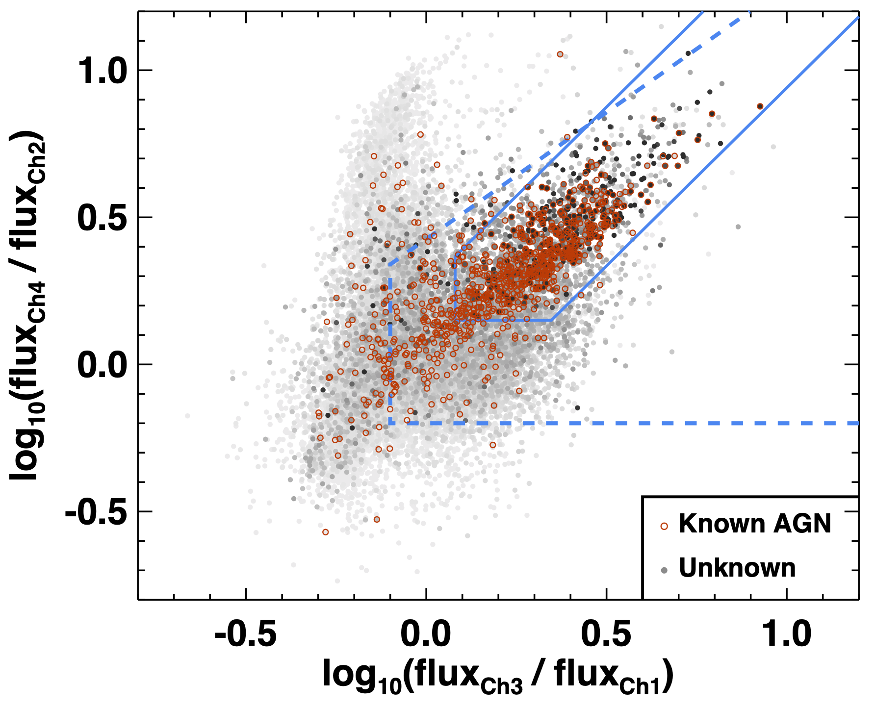
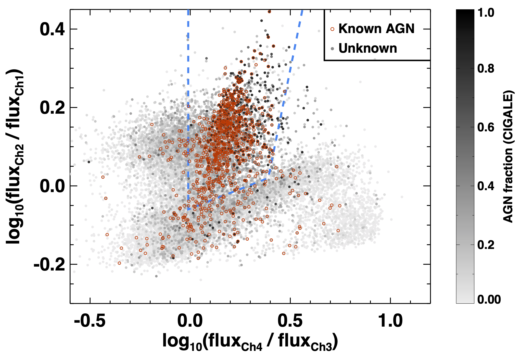
Figure 2: The location of the LoTSS-Deep sources on the Lacy et al. (2004) and Donley et al. (2012, left) and on the Stern et al. (2005, right) mid-IR colour-colour classification plots (for sources with S/N$>$2 in all four bands), in the Boötes field. The blue dashed lines on the left-hand panel show the Lacy et al. selection criteria, and the blue solid lines show those of Donley et al. On the right-hand plot, the Stern wedge is shown by the blue dashed lines. In both plots, the greyscale colour-coding indicates the AGN fraction from the cigale SED fitting using the skirtor AGN model. Objects confirmed to be AGN through optical spectroscopy or X-ray observations are indicated by the red circles.

Lacy et al. (2004) and Stern et al. (2005) derived the first colour-cuts based on shallow Spitzer data (hereafter referred to as the Lacy and Stern regions, respectively), and these were effective in separating out AGN from the population of relatively nearby inactive galaxies. However, the broad colour regions selected in these papers are heavily contaminated by higher redshift ($z>0.5$) inactive galaxies, that deeper Spitzer surveys (such as those available in the LoTSS Deep Fields) are able to detect. Donley et al. (2012) therefore defined a much tighter region of mid-IR colour space (hereafter, the Donley region) within which AGN samples display much lower contamination, but consequently are also less complete. Even in these deep datasets, however, fainter galaxies often lack measurements in one or more channels, preventing any classification by the Stern, Lacy or Donley criteria. To help overcome this, Messias et al. (2012) derived a series of redshift-dependent colour cuts based on K-band to Channel 2, Channel 2 to Channel 4, or Channel 4 to 24$\mu$m flux ratios (hereafter, the Messias regions). These allow classification of a larger fraction of galaxies, but with the same issues regarding completeness and contamination. Furthermore, simple application of colour cuts takes no account of low signal-to-noise measurements which can scatter data across the colour criteria, and can also miss some types of AGN (e.g. Gürkan et al., 2014).

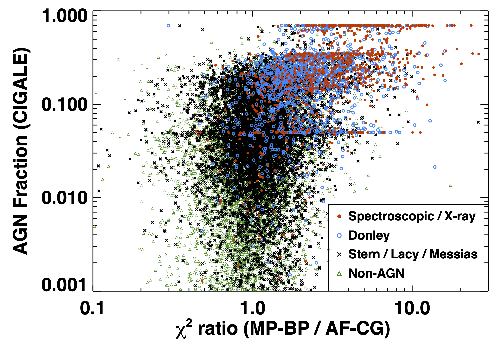
Figure 3: The cigale skirtor AGN fraction plotted against the ratio of the $\chi^{2}$ values between SED codes that do not include AGN components (the lower value for the magphys (MP) and bagpipes (BP) fits) and those that do (the lowest of the cigale (CG) and agnfitter (AF) fits), for the LoTSS-Deep sources in Boötes. Points are colour-coded according to whether they are spectroscopic or X-ray AGN (red filled circles), or satisfy the Donley criteria (with S/N$>$3 in each band; blue open circles), or satisfy the broader Stern, Lacy or Messias cuts (with S/N$>$3; black crosses), or ‘non-AGN’ that either do not satisfy any cuts or have too low signal-to-noise in the mid-IR for this to be determined (green triangles). The clustering at certain cigale AGN fraction values (e.g. 0.05, 0.7) appears to be a feature of the code, perhaps due to the fairly limited sampling of the grid of AGN model parameters. The plot shows that as the cigale AGN fraction rises above $\sim$0.1, objects are more likely to be identified as AGN through spectroscopic or X-ray selection or the Donley mid-IR cuts, and also that the SED fitting begins to deteriorate (higher relative $\chi^{2}$) for SED codes that don’t include AGN components.

The wide array of data available in the LoTSS Deep Fields allows a classification scheme to be developed which uses much more than just the mid-IR colour bands. The SED fitting described in the previous section encodes all of the mid-IR spectral expectations used in the Stern, Lacy, Donley and Messias colour criteria, but combines this with additional near-IR and optical data which allow simultaneous characterisation of the host galaxy properties; the latter allows the contribution of the host galaxy to the mid-IR to be directly predicted, and thus any additional AGN contribution to be more clearly distinguished. As an indication of this, Figure 2 shows the Stern, Lacy and Donley mid-IR colour-colour plots with the LoTSS-Deep sources in Boötes colour-coded by their AGN fraction as derived by cigale using the skirtor model. Sources classified as an AGN through optical spectra or X-ray properties are indicated in red. It can be seen that the X-ray and spectroscopically selected AGN and the objects with high cigale AGN fractions concentrate primarily in the selected colour-space regions, especially the Donley region, but that a significant fraction of these probable AGN are also found outside of these regions. Furthermore, there are objects within the colour-cuts (especially the broader Lacy and Stern regions) for which cigale predicts very low AGN contributions to the mid-IR.

The use of the four SED fitting routines provides two routes to identifying the probable AGN. First, each of cigale and agnfitter provides an estimate of $f_{\rm AGN}$, the fractional AGN contribution to the mid-IR. Second, objects which have a significant AGN contribution to their SED should be poorly fitted using magphys or bagpipes (and typically better fitted using cigale or agnfitter). Figure 3 demonstrates these effects, by showing the cigale AGN fraction plotted against the ratio of the $\chi^{2}$ values determined from the SED fits without AGN components compared to those with AGN components, with points colour-coded by evidence for AGN from either spectroscopic or X-ray data, or from mid-IR colour cuts. The spectroscopic and X-ray selected AGN generally show both moderate-to-high AGN fractions and a higher $\chi^{2}$ using magphys/bagpipes than using cigale/agnfitter. The majority of objects which lie securely within the Donley mid-IR colour-cuts show the same characteristics. Objects that lie only within the broader Stern, Lacy or Messias colour regions typically show much lower AGN fractions and the $\chi^{2}$ value from the magphys/bagpipes fits is lower than or comparable to that from cigale/agnfitter; they largely overlap with the ‘non-AGN’ that either lie outside of these colour cuts or do not have sufficiently high signal-to-noise in their mid-IR measurements for this to be determined. Nevertheless, the SED fits are able to pick out promising AGN candidates within these categories.

An examination of the AGN fractions derived by cigale and especially by agnfitter shows that many of these have quite large uncertainties, especially for fainter galaxies with fewer securely-measured photometric points. Investigations indicated that the 16^th percentile of the posterior of the AGN fraction (i.e. the 1-sigma lower limit on the AGN fraction; hereafter P16) provided a more robust indication of the presence of an AGN. The selection of radiative-mode AGN was therefore made by considering three selection criteria (see below for a discussion of how the threshold values were set):

1. whether the P16 AGN fraction from cigale, using the skirtor AGN models, exceeded a threshold value of 0.06 (ELAIS-N1 and Lockman Hole fields) or 0.10 (Boötes field).

2. whether the P16 value for the AGN fraction from agnfitter, as defined in Eq. 1, exceeded a threshold value of 0.15 (ELAIS-N1 and Lockman Hole fields) or 0.25 (Boötes field).

3. if the lower of the reduced $\chi^{2}$ values arising from the magphys and bagpipes SED fits was both greater than unity and at least a factor $f$ greater than the lowest of the reduced $\chi^{2}$ values arising from the two cigale and the agnfitter SED fits. The factor $f$ was determined to be twice the median value of the $\chi^{2}$ ratio between the better fit from magphys and bagpipes and the best fit from cigale and agnfitter(cf. Figure 4). This evaluated to $f=1.36$ for ELAIS-N1, $f=1.59$ for Lockman Hole and $f=2.22$ for Boötes.

An object was classified as a radiative-mode AGN if it satisfied at least two of these three criteria. In practice, this means either that it has a determined high AGN fraction from both cigale and agnfitter  or it has a high AGN fraction from at least one of the two codes combined with a superior SED fit using methods which include AGN components. The selection cuts for each criterion were set by comparing the derived classifications with the spectroscopic and X-ray samples and considering the locations of the classified AGN and non-AGN on mid-IR colour-colour diagrams. The threshold values selected were different for Boötes than for the other two fields. This is because the AGN fractions calculated in that field were systematically higher than those in ELAIS-N1 or Lockman Hole (e.g. a median AGN fraction of 0.037 in Boötes using the cigale skirtor model, compared to 0.029 in each of ELAIS-N1 and Lockman), which is likely to be due to the different manner in which the photometric catalogues were constructed in Boötes (see Paper III, ). Setting higher thresholds in Boötes ensured a consistency of classification across the three fields (cf. Sec. 7). Finally, a small proportion of objects did not meet these criteria but had previously been identified to be an AGN based on either optical spectra or X-ray properties; these were added to the radiative-mode AGN sample (and correspond to about 3 per cent of all radiative-mode AGN).

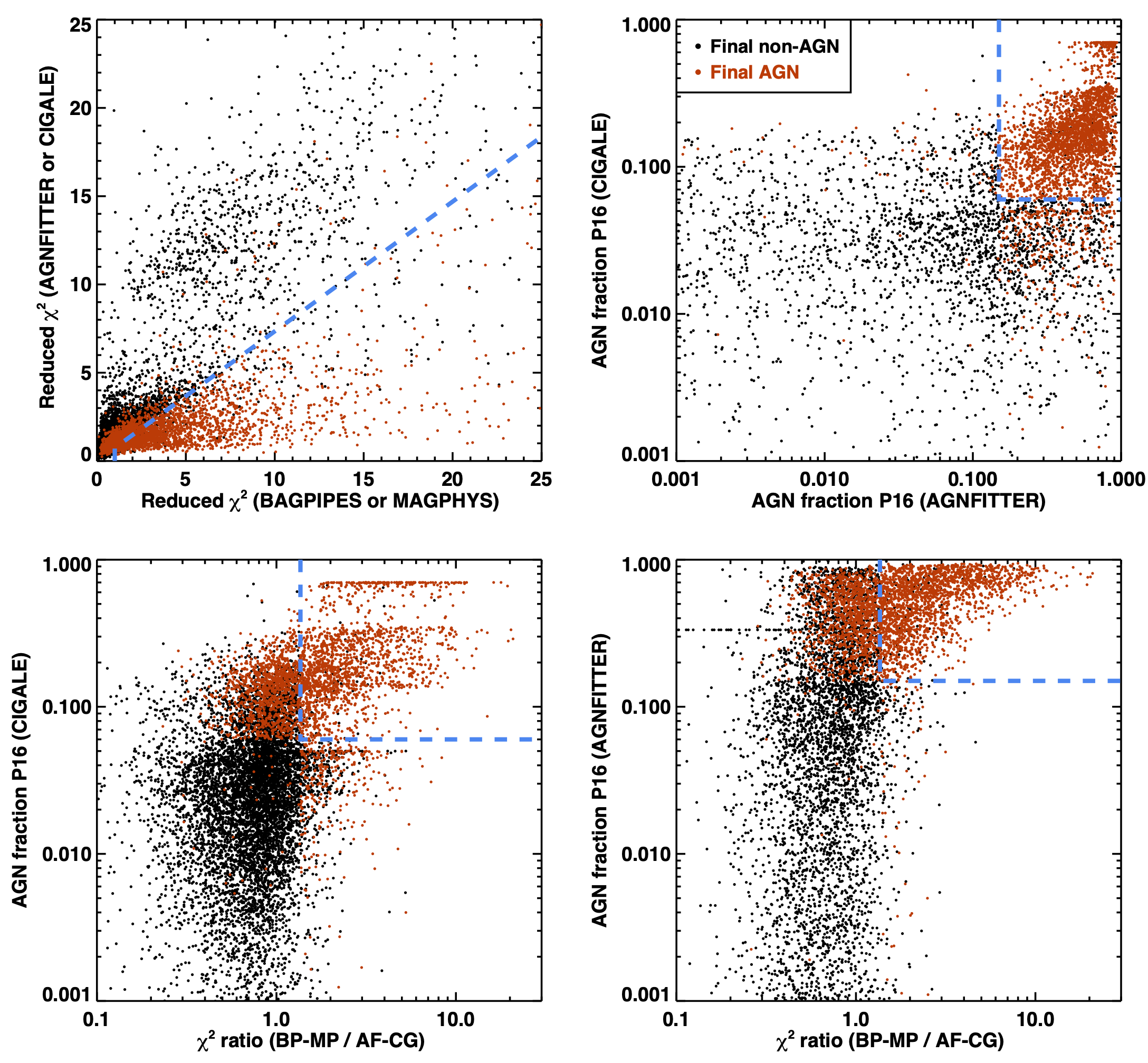
Figure 4: The selection criteria used to identify radiative-mode AGN, and the relative distributions of the AGN and non-AGN thus identified. The upper-left panel compares the reduced $\chi^{2}$ value resulting from SED models including an AGN component (agnfitter, cigale) against those which do not (magphys, bagpipes), with the blue dashed line showing selection criterion (iii). The upper right plot shows the 1-sigma lower limits (16^th percentile; P16) to the AGN fraction from agnfitter and cigale (with the skirtor AGN model), with the blue dashed lines showing selection criteria (i) and (ii). The lower plots show selection criteria (i) vs (ii) and (i) vs (iii) in the left and right panels respectively. Data shown are for ELAIS-N1. Sources are selected as radiative-mode AGN if they satisfy at least two of the three criteria (or are confirmed AGN from spectroscopic or X-ray observations): these sources are shown in red.

Fig. 4 shows the LoTSS-Deep sources on different combinations of these selection criteria, with the sources that satisfy at least two criteria, and therefore are selected as radiative-mode AGN, shown in red. It can be seen that there is a broad consistency between the different criteria: most of the selected radiative-mode AGN satisfy all three criteria and therefore are secure classifications. The main addition to this is a population of sources selected as having high AGN fractions by both cigale and agnfitter but with comparable, low $\chi^{2}$ values from the different fitting methods; these are probably sources where cigale and agnfitter are able to pick out a weak AGN through the mid-IR emission, but there is little-to-no direct AGN light through the optical to near-IR spectrum and so magphys and bagpipes are still able to provide a good fit to the majority of the spectrum.

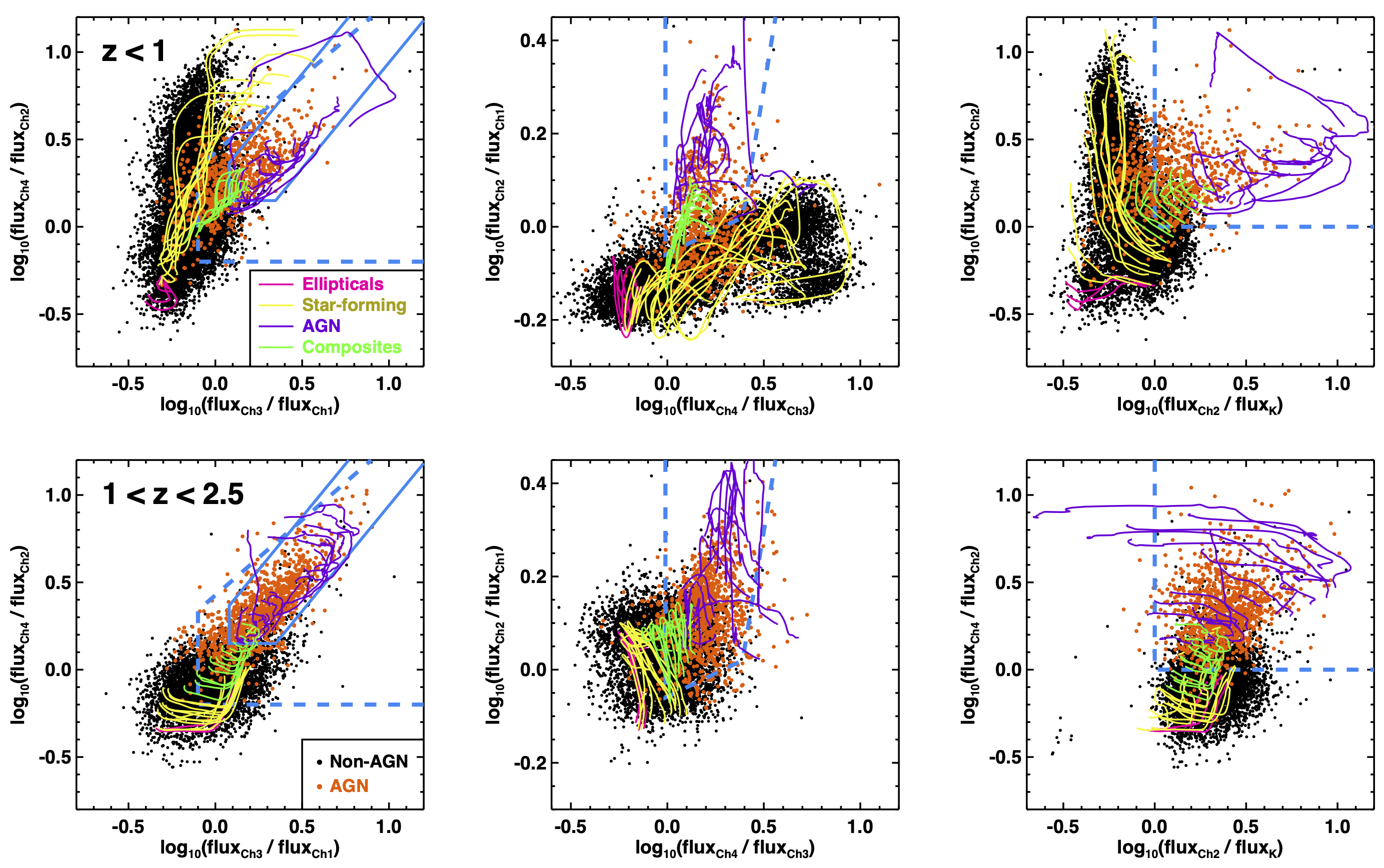
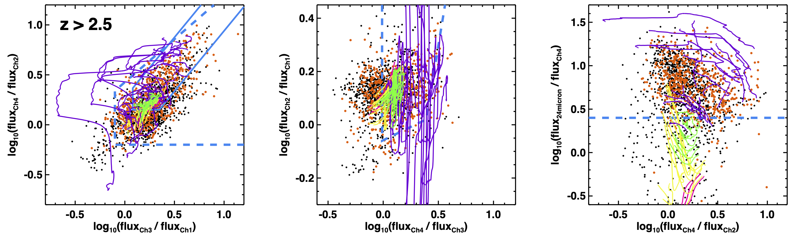
Figure 5: Infrared colour-colour plots for the LoTSS-Deep sources in ELAIS-N1, compared with template spectra. The sources classified as (radiative-mode) AGN are plotted in red and the non-AGN in black symbols; sources are only plotted if they have a signal-to-noise of at least 3 in each of the relevant filters. For clarity, sources (and templates) are divided into three redshift ranges: the top row is for $z<1$, the middle row for $1<z<2.5$ and the bottom row for $z>2.5$. For each redshift, the left-hand plot shows the mid-IR IRAC flux ratios used for the Lacy et al. (2004, blue dashed lines) and Donley et al. (2012, blue solid lines) selections. The middle column shows the Stern et al. (2005) colour criteria, with the Stern region indicated by the blue dashed lines. The right-hand column shows the selection criteria proposed by Messias et al. (2012), combining IRAC colours with the K-band flux at the lower redshifts, and with the 24$\mu$m flux at the highest redshifts. In each plot the coloured lines indicate the evolution over the specified redshift range of a selection of galaxy and AGN template spectra, from Brown et al. (2014) and Brown et al. (2019), separated into ellipticals (pink), star-forming galaxies (yellow), AGN (purple), and composites (green). As can be seen, the broad colour cuts suffer to various extents from both incompletensss and contamination. The selected AGN broadly align with the regions of colour space covered by the AGN and composite template spectra.

Fig. 5 shows the selected radiative-mode AGN and non-AGN on a series of mid-IR colour-colour diagrams, compared against the evolving colours of various galaxy template models. The panels are split by redshift ranges, in order to allow a clearer comparison against the template expectations. At each redshift, the panels show the Lacy and Donley colour plots (left), the Stern colour plot (middle), and the appropriate Messias plot (right). Template SED models were drawn from the ‘Galaxy SED Atlas’ of Brown et al. (2014) combined with the ‘AGN SED Atlas’ of Brown et al. (2019). SEDs were selected from these libraries for: (i) elliptical galaxies (as expected to be seen for jet-mode AGN); (ii) star-forming galaxies; (iii) AGN (including both quasars and edge-on ‘type-II’ AGN); and (iv) composite spectra, produced by combining a set of Seyfert AGN spectra with host galaxy spectra, with a range of weights.

The template tracks for the different galaxy classes confirm both the motivation for, and the shortcomings of, the colour-colour selection criteria: the Donley region relatively cleanly selects AGN at $z<2.5$ but is incomplete for composite systems; the Stern and Lacy regions are more complete for composite systems but contaminated, especially at the higher redshifts; the Messias cuts perform relatively well, especially at the highest redshift where the use of the 24$\mu$m colour gives a clear advantage, but still have some incompleteness and contamination. The red points show the objects selected as radiative-mode AGN by the techniques outlined above. At all redshifts these broadly overlap the regions of the AGN and composite templates, extending where appropriate beyond the colour-selection limits. It is clear, however, that in the $z>2.5$ redshift range there remains a significant population of objects that are not classified as AGN, and yet which lie in similar regions of colour-space to the AGN. At these redshifts, as is evident from Fig. 5, it is only the Channel 4 and 24$\mu$m filters that are able to probe rest-frame wavelengths where an AGN template becomes clearly distinct from the galaxy templates, and the composites are even more difficult to distinguish. Especially with the typically low signal-to-noise of the galaxies in this highest redshift bin, the SED fitting techniques may be less reliable: although the classifications are provided for all sources, readers should treat these with caution at $z>2.5$, where there may well be a degree of incompleteness in the AGN sample.

5 Comparison of derived properties and consensus measurements

Two of the most important galaxy properties to determine are the stellar mass and the star-formation rate. Each of the SED fitting codes provides an estimate of these parameters. This section discusses how these values are combined to produce consensus measurements for each source.

In brief summary, for sources which do not host an AGN, the magphys and bagpipes codes ought to provide the best measurements of mass and SFR, because these models offer a significantly broader selection of galaxy templates. Indeed, for these sources, the results from these two codes show excellent agreement in their estimates of both stellar mass (median absolute difference of just 0.09 dex) and SFR (0.14 dex). The consensus values of the stellar mass and SFR for non-AGN were therefore generally derived from the logarithmic mean of the magphys and bagpipes results.

For radiative-mode AGN, the magphys and bagpipes results are potentially unreliable as they do not include any AGN component in their SED modelling. The two cigale runs (with the Fritz and skirtor AGN models) should be more reliable, and indeed these two agree with each other well: the median absolute difference is only 0.09 dex in stellar mass and 0.13 dex in SFR. agnfitter is found to provide less consistent results, but is valuable for the small fraction ($\approx 2$ per cent) of sources which are highly AGN-dominated, and for which agnfitter’s superior modelling of the AGN UV emission is required. The consensus values of the stellar mass and SFR for radiative-mode AGN were therefore typically derived from the logarithmic mean of the two cigale results, except where cigale failed to provide an acceptable fit, in which case the agnfitter values were adopted.

Sections 5.1 and 5.2 now provide (for stellar mass and SFR respectively) a much more detailed comparison of the outputs of the different SED fitting codes, along with a full description of how the generalised approach discussed above was adapted in cases where one or more of the SED codes failed to provide an acceptable fit. Readers not interested in these finer details may wish to skip to Section 6.

5.1 Consensus stellar masses

For sources which are not identified to be a radiative-mode AGN, the results from the magphys and bagpipes codes show excellent agreement in their estimates of stellar mass: where both magphys and bagpipes pass the threshold for an acceptable fit (see Section 3.4) the median absolute difference in stellar mass is just 0.09 dex, with over 90 per cent of sources agreeing within 0.25 dex; the outliers are generally the faintest sources, at low masses or high redshifts. cigale also gives very similar values, with a median difference in stellar mass of only 0.11 dex, and over 85 per cent agreeing within 0.25 dex. agnfitter shows much lower agreement, however, with a median difference in stellar mass of 0.27 dex compared to the estimates from the other codes. This inconsistency for agnfitter is likely to be associated with the lack of an energy balance in the fitting process.

For these non-AGN the consensus stellar mass was derived from the mean of the logarithm of the stellar masses derived using magphys and bagpipes, as long as both codes provided an acceptable fit to the data ($\approx 86$ per cent of the non-AGN, though rising to nearly 95 per cent in ELAIS-N1). If one of the two codes provided a bad fit and the other a good fit (11 per cent of cases), then the stellar mass estimate from the well-fitting code was adopted as the consensus measurement. If both codes produced fits below the acceptability threshold then the values of the two stellar mass estimates were examined: if they agreed with each other within 0.3 dex ($\approx 2$ per cent of cases) then it was likely that the unreliability of the SED fits was driven by some outlier points that did not invalidate the stellar mass estimates, and so the logarithmic mean of the two values was adopted as the consensus stellar mass. If the two values disagreed by more than 0.3 dex, then the stellar mass estimates of the two cigale fits were examined as well: if the full range of all 4 stellar masses was less than 0.6 dex ($\approx 0.3$ per cent of cases) then the logarithmic mean of the four measurements was adopted as the consensus measurement; if the range was larger than 0.6 dex ($\approx 0.6$ per cent of sources) then it was deemed that no reliable stellar mass could be provided. A comparison of the consensus masses derived against the estimates from each code individually is shown by the black points in Fig. 6, confirming visually the good agreement of the magphys and bagpipes codes, broad agreement of cigale, and larger scatter of agnfitter for these sources.

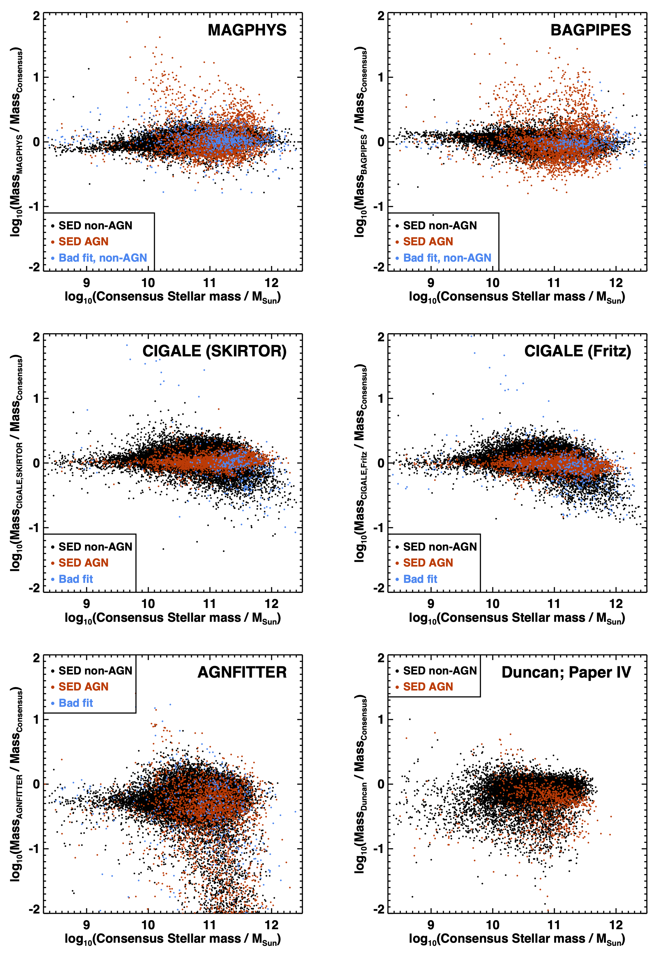
Figure 6: A comparison of the masses derived by the different SED fitting codes against the final consensus masses for the LoTSS Deep Field sources in ELAIS-N1. magphys, bagpipes and cigale all give broadly consistent results for non-AGN, but differ for the AGN subset, for which the cigale results should be more reliable. agnfitter masses show a small systematic offset compared to the other codes, and more outliers at high mass. The lower right plot examines the masses produced in Paper IV (only out to $z<1.5$); these are seen to give consistent results with only slightly larger scatter. This is of interest because these stellar masses were produced for the entire galaxy population in these deep fields, not just the LoTSS-Deep host galaxies.

For radiative-mode AGN, the two cigale runs provide stellar mass estimates that agree well with each other: the median absolute difference is only 0.09 dex, with 90 per cent of sources within 0.3 dex. Compared to these values, as expected, the results from magphys and bagpipes show greater scatter (each 0.16 dex median difference) and also a larger fraction of outliers where the codes significantly over-estimate the mass due to AGN light being incorrectly modelled as stellar emission (cf. Fig. 6). Again, agnfitter shows a larger dispersion in stellar mass measurements relative to the other codes, with a median absolute difference of 0.49 dex; this may be due to the stellar component being fitted independently without an energy balance constraint, with some stellar light perhaps being incorrectly modelled as AGN emission or vice versa, although it could also be related to the different approach to modelling the AGN emission. For these reasons, for the radiative-mode AGN, if both cigale runs provided acceptable fits then the logarithmic mean of the stellar masses from these two runs was accepted as the consensus mass (with agnfitter excluded due to its higher proportion of outliers); this was the case for just over 94 per cent of the radiative-mode AGN. Otherwise, if just one of the cigale runs provided an acceptable fit ($\approx 3$ per cent of cases) then the stellar mass from that run was adopted. If neither cigale run provided a good fit, but agnfitter did, then there was a likelihood that this was a case where either energy balance was breaking down or the superior modelling of the AGN UV emission by agnfitter was helping the fit; in these 2 per cent of cases, the agnfitter stellar mass estimate was used. Otherwise, it was decided that no reliable stellar mass estimate was possible.

Fig. 6 shows a comparison on each mass estimate against the consensus mass derived, and illustrates the trends discussed above. The lower-right panel also compares the consensus masses against those derived in Paper IV using a grid-based SED fitting mechanism (see also Duncan et al., 2019). This comparison is interesting because the stellar masses in Paper IV are derived for all galaxies in the field, not only the radio sources, and therefore allow a comparison between the radio sources and the underlying population. In Paper IV it is argued that the stellar mass estimates are only reliable out to $z\sim 1.5$, and so this is set as an upper limit for the plotted points. As can be seen, the agreement between the Paper IV stellar masses and the consensus masses derived here is very good for the non-AGN, with no significant systematic offset ($<0.1$ dex) and a median scatter of 0.11 dex. The performance for AGN is slightly worse, but still good, with a median scatter of 0.23 dex. These results confirm that the Paper IV masses provide reliable measurements for the broader population that can be used in comparison against the consensus masses for the radio source population.

In this paper, no attempt is made to derive uncertainties on the consensus stellar masses for individual sources. Uncertainties arise both due to statistical errors in the individual fits and systematic effects between different SED codes. Each SED code offers an estimate of its statistical uncertainty for each source, and the difference between the stellar masses from different SED codes can be used to gauge the size of the systematic errors. Another source of error is that during the SED fitting the redshift of the source is fixed at the best photometric redshift (unless a spectroscopic redshift is available): uncertainties in the photometric redshift are likely to be a significant contributor to the mass uncertainty for any given source. Instead of calculating uncertainties for individual sources, therefore, the approach taken here is to derive characteristic uncertainties on stellar mass as a function of the galaxy’s mass and redshift. The characteristic uncertainties are evaluated in Appendix A, and are found to be typically around 0.1 dex for higher mass sources at $z<2$, increasing towards higher redshifts and lower masses.

5.2 Consensus SFRs

Estimation of consensus SFRs follows broadly the same principles as those of the stellar masses, in the preferred use of the magphys and bagpipes results for the non-AGN and with the cigale results generally used for the AGN. As would be expected (cf. Pacifici et al., 2023), the agreement in SFR estimates between the different codes is not quite as good as that of stellar masses, but still strong. For non-AGN, the SFR estimates of magphys and bagpipes show systematic differences of less than 0.1 dex, with a median scatter of only 0.14 dex and over 75 per cent of cases agreeing within 0.3 dex. The cigale measurements agree comparably well at large SFRs, but frequently provide higher SFR estimates than either bagpipes or magphys at lower SFRs. agnfitter suffers from a significant systematic offset of, on average, more than 0.3 dex higher SFRs than the other estimators. For the radiative-mode AGN, the two cigale SFR estimations show good agreement with each other (median difference 0.13 dex). Both magphys and bagpipes systematically over-estimate the SFRs of these radiative-mode AGN, by around 0.15 dex on average. Fig. 7 provides a visual illustration of these effects.

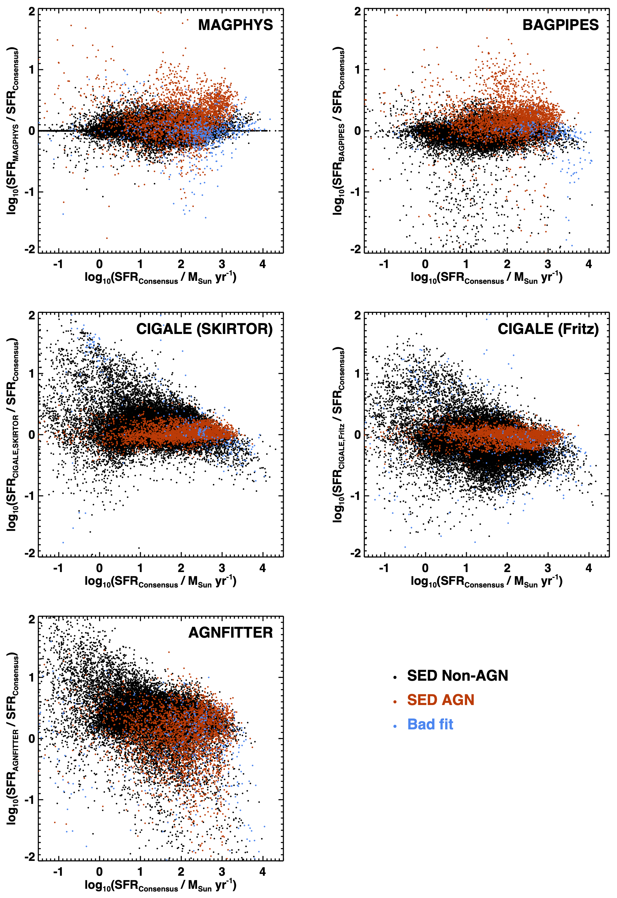
Figure 7: A comparison of the star-formation rates derived by the different SED fitting codes against the final consensus value, for the LoTSS Deep Field sources in ELAIS-N1. magphys and bagpipes give broadly consistent results for non-AGN; their performance on objects identified as (radiative-mode) AGN is more mixed, but generally reasonable where the fit is not flagged as a bad fit. cigale’s SFR estimations for non-AGN generally perform well at higher SFRs (especially with the skirtor AGN model), but over-predict the SFR in some lower-SFR galaxies. The estimated SFRs of objects selected as AGN show a high degree of consistency between the two different cigale runs. agnfitter SFRs show more scatter and a small systematic offset compared to the other codes.

To determine the consensus SFRs, like for stellar masses, the outputs from magphys and bagpipes are primarily considered for the non-AGN. The only significant difference in approach arises because of a small proportion of sources (around 9 per cent of all the non-AGN sources, mostly at lower SFRs) for which bagpipes returns an acceptable fit, but the SFR is dramatically below that of magphys and with an uncertainty that can be several orders of magnitude larger than the estimated value. These very low SFRs arise because of the parametric (exponentially-declining) form of the bagpipes SFR history, which can lead to unrealistically-low best-fit SFRs at large ages where the e-folding time is short, but with considerable uncertainty. For these sources, the cigale SFR estimates are found to broadly agree with the magphys values, with both often within the 1$\sigma$ confidence interval of the bagpipes fit. Therefore, sources for which the bagpipes fit is deemed to be good, but the uncertainty on the bagpipes SFR estimate is more than 5 times the estimate itself, are treated differently. In these cases, if magphys provides an acceptable fit then the magphys estimate is adopted as the consensus value; if it does not, but the magphys and cigale estimates agree within 0.5 dex then the logarithmic mean of the magphys and cigale values is taken as the consensus value; otherwise, the results are deemed inconsistent and no consensus SFR is derived. Other than these cases, the approach to derive consensus SFRs for the non-AGN exactly matches that for deriving stellar masses. Similarly, for the radiative-mode AGN, the approach for stellar masses using cigale (or occasionally agnfitter) estimates is replicated for the SFRs.

Fig. 7 compares the consensus SFRs against the estimates from each individual code. The spread in derived values between different codes is comparable to that in the analysis of Pacifici et al. (2023). As with stellar masses, no attempt is made to provide a source-by-source uncertainty on the consensus SFR, but Appendix A discusses the typical errors; except for the few per cent of lowest-SFR objects at each redshift (where the uncertainties increase greatly), these can be broadly approximated as $\Delta$(SFR) $\approx 0.1(1+z)^{0.5}$ dex.

6 Identification of radio AGN

As discussed in the introduction, star-forming galaxies show a tight correlation between their radio luminosity and their SFR. This relation allows the identification of sources which possess significant radio emission associated with AGN activity, as they will appear offset to larger radio luminosities than would be predicted from their SFR (cf. Delvecchio et al., 2017; Williams et al., 2018; Whittam et al., 2022). Relationships between SFR and low frequency radio luminosity have been previously derived at relatively low redshifts by Calistro Rivera et al. (2017), Brown et al. (2017), Gürkan et al. (2018) and Wang et al. (2019), and most recently by Smith et al. (2021) using the LoTSS-Deep data in ELAIS-N1. As discussed by Smith et al., in order to determine an accurate relation it is essential to properly account for non-detections, otherwise there is a risk that the derived relation will be dependent on the depth of the radio imaging, with the bias decreasing as the depth of the radio imaging increases. Smith et al. derive their relationship out to $z\approx 1$ using a near-IR magnitude selected sample, finding $\log_{10}L_{\rm 150MHz}=22.22+1.06\log_{10}({\rm SFR})$ for the sample as a whole (where $L_{\rm 150MHz}$ is in units of W Hz^-1 and SFR in units of $M_{\odot}$ yr^-1), based on SFRs derived using magphys.

In this paper, the use of the consensus SFRs, and the extension to higher redshifts, may be expected to lead to small changes in the best-fit relation. A suitable relation is therefore derived using a ‘ridgeline’ approach. In this approach, the sources are binned into different (narrow) bins in SFR, and within each bin the distribution of radio luminosities of the detected sources is examined. The peak of the distribution is identified as the ridgeline point. Provided the radio survey is sufficiently deep then, especially in the presence of a distorted distribution (the star-forming population plus a distribution of radio-excess AGN), this method should provide a more reliable value than the mean or median of the distribution of detected sources. The radio luminosities and SFRs of the LoTSS-Deep sources are shown in the upper panel of Fig. 8, along with the calculated ridgeline points, which can be well-fitted by the relation

$$\log_{10}(L_{\rm 150MHz}/{\rm W\,Hz}^{-1})=22.24+1.08\log_{10}({\rm SFR}/{\rm M}_{\odot}\,{\rm yr}^{-1})$$ (2)

The uncertainty on the ridgeline gradient is $\pm 0.06$, and the uncertainty on the intercept at $\log_{10}({\rm SFR})=1.5$ (the median value, where the errors on the gradient and intercept are uncorrelated) is $\pm 0.07$. To within 1$\sigma$, there is no difference in this relation between those sources classified as radiative-mode AGN or not. The relation derived from the ridgeline is fully consistent with that of Smith et al. (2021), agreeing within 0.1 dex over the full range of star-formation rates probed.

The distribution of radio luminosities below the ridgeline can be reasonably well-fitted by a Gaussian distribution of width 0.22 dex; this also holds in different bins of star-formation rate, with the Gaussian width remaining constant (to $\pm 0.02$ dex) from low to high SFR. The distribution above the ridgeline shows a much more extended tail, as expected. In ELAIS-N1 and Lockman Hole, radio-excess sources are here defined as those sources with radio luminosities exceeding the ridgeline value by 0.7 dex, corresponding to approximately 3$\sigma$. It should be noted that this limit corresponds to approximately 0.8 dex above the relation of Smith et al. (2021) at high SFR; these authors derived a scatter in their relation of around 0.3 dex at ${\rm SFR}>10M_{\odot}$yr^-1 (at lower SFRs they measured lower scatter, but noted that this might be due to the limiting depth of the radio imaging); Cochrane et al. (2023) also derive a similar value for the scatter. Therefore, the radio-excess selection adopted here also broadly corresponds to a 3$\sigma$ excess relative to the Smith et al. relation. In Boötes (where the input photometry was different), it is found that the scatter in the SFR-radio relation increases towards higher redshifts, and adoption of a fixed 0.7 dex cut-off leads to an excess of radio-AGN at higher redshifts compared to the other two fields. To remedy this, in Boötes the radio excess threshold is modified slightly to ($0.7+0.1z$) dex, which brings the classifications in this field in line with those in ELAIS-N1 and Lockman (cf. Fig 9).

There is a small population of radio sources with consensus SFRs well below $0.01M_{\odot}$yr^-1. SFRs at this level cannot be accurately estimated by the SED fitting codes, and thus have large associated uncertainties. This makes a radio-excess classification based on the consensus SFR potentially unreliable for these sources. To avoid this issue, these sources were only classified as radio-excess if their radio luminosity exceeded (by 0.7 dex) that expected for a SFR of $0.01M_{\odot}$yr^-1. If their radio luminosity was below that level, but above the radio-excess limit for their estimated consensus SFR, they were deemed to be unclassifiable in terms of radio excess (0.4 per cent of sources).

Finally, a small proportion of sources do not reach the radio-excess selection threshold, but are clearly extended or multi-component radio sources, inconsistent with simply being star-forming galaxies. Those sources which are either multi-component sources associated through the LOFAR Galaxy Zoo effort (Paper III) with a physical size in excess of 80 kpc, or single component sources with a major axis size in excess of 80 kpc and which also exceed the resolved source threshold defined in Shimwell et al. (2019) by at least a factor of 1.5, were deemed to be clearly extended. These sources were added to the radio-excess sample if they were not already included (just under 0.5 per cent of the sample).

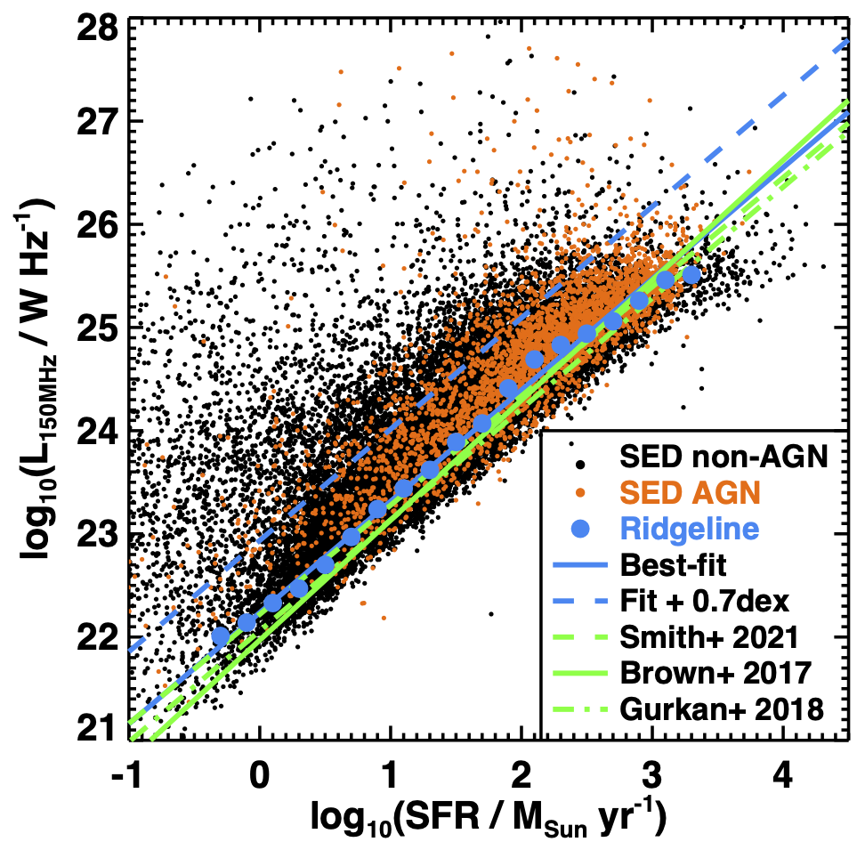
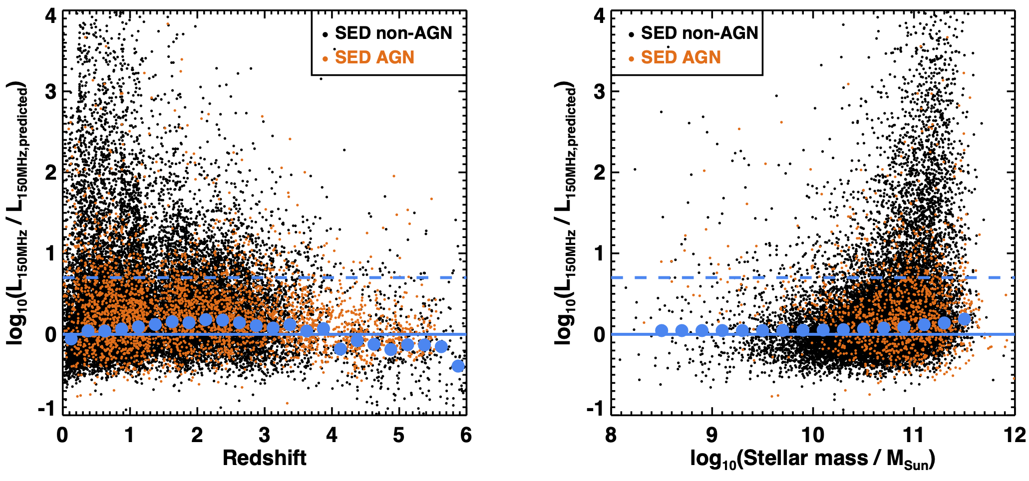
Figure 8: Top: the distribution of radio luminosity versus SFR for LoTSS Deep Field sources in ELAIS-N1, split into those identified as radiative-mode AGN from their SED (red points) and the sources which are not radiative-mode AGN (‘SED non-AGN’; black points). Within narrow bins in SFR, the ‘ridgeline’ points (larger blue circles) indicate the peak of the distribution of radio luminosities. These can be well-fitted by a power-law distribution shown by the solid blue line, which is in broad agreement with literature relations (green lines). Bottom: the ratio of observed radio luminosity to that predicted from the consensus SFR based on the ridgeline fit, versus redshift (left) and stellar mass (right). The horizontal dashed lines represent the expected relation and the radio-excess threshold. Solid blue points in each plot show the peak of the distribution in narrow bins. These always lie within 0.2 dex of the expected relation. Radio-excess sources are found over the full range of redshifts, but predominantly concentrate at high stellar masses.

The lower panels of Fig. 8 show the ratio of measured radio luminosity over that expected from the consensus SFR as a function of redshift (left) and stellar mass (right); the horizontal dashed lines show the expected relation for star-forming galaxies and the radio-excess threshold, and the blue circles indicate again the peak of the distribution at each redshift. It can be seen that there is a weak variation of the population distribution with redshift, but no consistent trend, and the distribution peak never moves more than 0.2 dex ($<1\sigma$) from the ridgeline value. Radio excess sources are found across all redshifts. The apparent gradual decline in the ratio with increasing redshift at $z>2.5$ may be due to an increasing incompleteness in the classification of radiative-AGN at these redshifts (see Sec. 4), leading to an over-estimate in the SFR of some sources.

Regarding stellar mass, it is immediately clear from the lower-right panel of Fig. 8 that the proportion of radio-excess sources increases very strongly with mass, in particular for those objects not selected to be radiative-mode AGN. This is the well-known trend that, in the local Universe, the radio-loud AGN fraction shows a very strong mass dependence (e.g. Best et al., 2005; Sabater et al., 2019). Kondapally et al. (2022) use this LoTSS-Deep sample to investigate the cosmic evolution of this trend. Fig. 8 also shows a weak variation of the peak of the distribution of observed-to-predicted radio luminosity with mass, with a consistent trend of higher mass galaxies having on average a slightly higher radio luminosity for a given SFR. This has been previously seen in the radio luminosity to SFR relation (e.g. Gürkan et al., 2018; Smith et al., 2021), but it remains unclear to what extent this is due to an intrinsic mass-dependence of the amount of radio emission arising from star formation, as opposed to the effect of a contribution from a population of radio-weak AGN, more prevalent at higher stellar masses, that fall below the selection limit for radio-excess sources.

Regardless, the variations in Fig 8 are sufficiently small (in both redshift and stellar mass) that the use of a single SFR-radio relation does not significantly affect the selection of radio-excess sources.

7 Final radio source classifications, and dependencies

In the previous sections, LoTSS-Deep sources have been identified as either radiative-mode AGN or not, and either radio-excess sources or not, with a small number of sources being unclassifiable in each case. Here, these are combined to derive a final set of source classifications.

• Sources which are neither radiative-mode AGN nor radio-excess sources are classified simply as star-forming galaxies (SFGs). Note that this may include some quiescent galaxies (with SFRs below the stellar mass vs SFR main sequence) whose low redshift nevertheless allows the star formation to be detected by LOFAR.

• Sources which are radiative-mode AGN but which do not display a radio excess are radio-quiet AGN (RQAGN; including the radio-quiet quasars)

• Sources which are not radiative-mode AGN but do display a radio excess are the population of jet-mode AGN. Traditionally these sources are referred to as low-excitation radio galaxies (LERGs)

• Sources which are both radiative-mode AGN and radio-excess sources are sources such as radio-loud quasars (Type I or Type II). These are traditionally referred to as high-excitation radio galaxies (HERGs).

• Finally, any source which could not be reliably classified in either of the criteria was left as unclassified.

Table 2: The number of sources of each class in the LoTSS-Deep DR1 dataset.

Source classification	ELAIS-N1	Lockman Hole	Boötes	Total	Percentage
Star-forming galaxies	22720	21044	11916	55680	67.9
Radio-quiet AGN	2779	2633	2030	7442	9.1
Low-excitation radio galaxies	4287	5304	3158	12749	15.6
High-excitation radio galaxies	510	710	524	1744	2.1
Unclassified	1314	1471	1551	4336	5.3
Total	31610	31162	19179	81951	100

Table 2 shows the number of sources of each class in each field. As can be seen, the majority population in LoTSS-Deep DR1 is the star-forming galaxies: these comprise just over two-thirds of the total population, rising to over 70 per cent in the deepest field, ELAIS-N1. Radio-quiet AGN contribute nearly 10 per cent of the total, with the two radio-loud classes contributing around 18 per cent between them, mostly as LERGs. Five per cent of the sources are unclassified. Of these, around 3 per cent are the sources without host galaxy identifications or redshifts for which no SED fitting could be carried out, and the remaining 2 per cent are mostly fainter galaxies for which the SED fitting algorithms either did not provide acceptable fits or provided highly inconsistent results.

Table 3 provides the first five lines of the classification data for each source in ELAIS-N1, along with the consensus mass and SFR measurements; the full catalogues for each field are provided electronically. More extensive catalogues, including the key outputs of each SED fitting code that were used to derive these, are made available on the LOFAR Surveys website (lofar-surveys.org).

Table 3: Classification results and consensus measurements for each source. The table shows the first five sources in ELAIS-N1: full catalogues are available electronically. Columns give the full source identifier, the radio ID number, the total 150 MHz flux density (in Jy), the redshift, the final radiative-mode AGN classification (1$=$AGN, 0$=$non-AGN, $-1$$=$unclassifiable), the logarithm of the consensus stellar mass (in solar masses), the logarithm of the consensus SFR (in solar masses per year), the radio excess (in dex), a flag to indicate extended radio sources (as defined in Sec. 6; 1$=$extended, 0$=$compact), the final radio-AGN classfication (1$=$radio-AGN, 0$=$no radio excess, $-$1$=$unclassifiable), and the overall classification (SFR$=$star-forming galaxies; RQAGN$=$radio-quiet AGN; LERG$=$low-excitation (jet-mode) radio galaxy; HERG$=$high-excitation (quasar-mode) radio galaxy; Unc$=$unclassified. Values of $-$99 indicate where no measurement is available.

Source Name	Radio ID	$S_{\rm 150MHz}$	$z$	AGN	log10(Mass)	log10(SFR)	Radio excess	Extended	Radio	Overall
		[Jy]		class	[M⊙]	[M⊙/yr]	[dex]		class	class
ILTJ155957.58+550052.4	0	0.000396	2.0437	0	11.62	2.22	0.31	0	0	SFG
ILTJ155958.25+550105.3	1	0.000736	0.6697	0	11.00	1.58	0.15	0	0	SFG
ILTJ155958.68+550534.6	2	0.000197	1.4289	0	11.58	1.16	0.79	0	1	LERG
ILTJ155959.52+545751.0	3	0.000158	1.7777	0	11.20	1.71	0.32	0	0	SFG
ILTJ160000.65+550723.3	4	0.000196	3.6960	1	11.42	2.87	-0.13	0	0	RQAGN
…	…	…	…	…	…	…	…	…	…

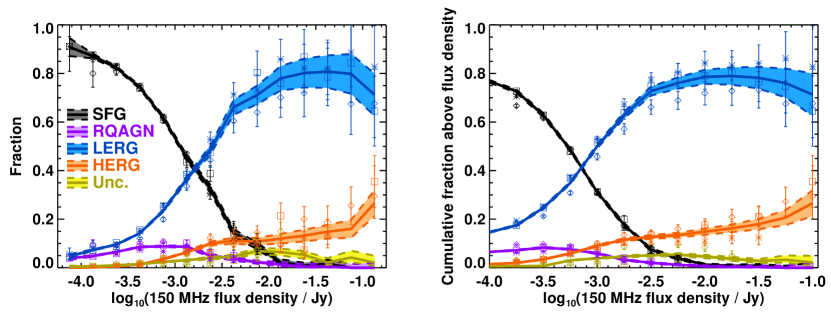
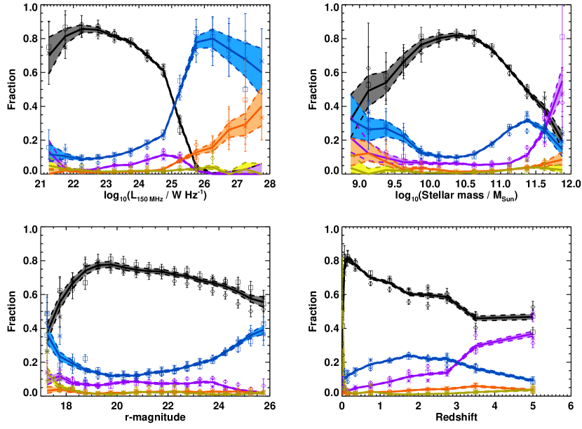
Figure 9: The fraction of sources of each different class (star-forming galaxies in grey; radio-quiet AGN in purple; low-excitation radio galaxies in blue; high excitation radio galaxies in orange; unclassifiable sources in yellow) as a function of radio flux density (upper panels; left gives fraction at a given flux density, and right gives cumulative fraction above a flux density), radio luminosity (middle left), stellar mass (middle right; for sources with $z<1.8$ only – see text), optical r-band magnitude (lower left) and redshift (lower right; out to a final bin of $4<z<6$). On each plot, the solid line for each class represents the derived fraction, and the shaded region indicates the calculated uncertainty. The open symbols show the values derived from each individual field (square $=$ ELAIS-N1; asterisk $=$ Lockman Hole; diamond $=$ Boötes), where there are at least 5 sources from that field in the given bin, and demonstrate the broad agreement between fields. Note that the rise of the radio-quiet AGN population at the highest stellar masses is probably an artefact of larger mass uncertainties for these sources; see text for details.

Figure 9 shows the distribution of the different classes of source as a function of various properties of the host galaxy. The top panels show the distribution with respect to the 150-MHz flux density: the left panel shows the fraction at a given flux density, and the right panel shows the cumulative fraction above a given flux density. The population is dominated by radio-loud AGN above flux densities of about a mJy. The bulk of these are the LERGs, but with the fraction of HERGs beginning to rise at the highest flux densities, where the coverage of the sample begins to run out due to lack of sky area for these rarer bright sources. This rise of the HERG population is seen even more starkly in the middle left panel, which shows the distribution as a function of radio luminosity, and is in line with expectations from the relative luminosity functions of these two populations (e.g. Best & Heckman, 2012; Best et al., 2014). At lower flux densities (and below 150 MHz luminosities of around $10^{25}$W Hz^-1), star-forming galaxies take over the sample and quickly become the dominant population, accounting for over 90 per cent of sources at the limiting flux density reached in ELAIS-N1 (and more than 75 per cent of the cumulative population above $S_{\rm 150MHz}\approx 100\mu$Jy). The switch between a star-formation dominated population and a radio-loud AGN dominated population occurs at around $S_{\rm 150MHz}\approx 1.5$ mJy, which is fully consistent with the switch point at higher frequency of $S_{\rm 1.4GHz}\approx 200\mu$Jy (found by Smolčić et al., 2017b) or $S_{\rm 1.4GHz}\approx 250\mu$Jy (found by Padovani, 2016), considering the typical radio spectral index of these sources.

At all flux densities below a few mJy there is a significant population of radio-quiet AGN, accounting for just under 10 per cent of all sources over the 100 $\mu$Jy to 1 mJy flux density range. This is slightly lower than the fraction found in observations at higher frequencies: early work by Simpson et al. (2006) suggested that 20 per cent of sources with 100 $\mu$Jy $\mathrel{\hbox to0.0pt{\lower 3.0pt\hbox{$\mathchar 536\relax$}\hss}\raise 2.0pt\hbox{$\mathchar 316\relax$}}S_{\rm 1.4GHz}\mathrel{\hbox to0.0pt{\lower 3.0pt\hbox{$\mathchar 536\relax$}\hss}\raise 2.0pt\hbox{$\mathchar 316\relax$}}300$ $\mu$Jy are radio-quiet AGN, while the COSMOS 3GHz work of Smolčić et al. (2017b) indicated between 15 and 20 per cent (as determined from the 70 per cent subset of their ‘High Luminosity AGN’ sample that shows no radio excess). The origin of this difference is not completely clear. It may be related to different implementations of the radio-loud to radio-quiet separation, but more likely is associated with the radio-quiet AGN having a flatter spectral index than star-forming galaxies (e.g. due to a greater proportional contribution of flatter-spectrum core emission) and therefore lesser prominence at the lower frequencies probed by LOFAR. Given the steepness of the radio source counts, a difference of only $\approx$0.2 in spectral index between star-forming galaxies and radio-quiet AGN would decrease the proportion of radio-quiet AGN in the sample by about a factor of 2; LOFAR studies of radio-quiet quasars provide evidence in support of such flatter spectral indices (e.g. Gloudemans et al., 2021).

The additional panels of Fig. 9 show the distribution of source classes as a function of redshift, stellar mass and optical magnitude. Note the strong rise of unclassified sources at $z<0.1$; low SFRs for these galaxies can also lead to ambiguous radio excesses, while in addition the aperture photometry and aperture corrections used for the LoTSS Deep Field photometry (Paper III) are not optimised for these low redshifts, and resulting errors will affect the SED fitting. At these redshifts, it is in any case better to use the shallower, wider-area LoTSS surveys. All populations are seen over the full range of optical magnitudes. As expected, the LERG population shows increasing importance at higher stellar masses (note that this panel only includes redshifts $z<1.8$ as mass estimates become increasingly less reliable at higher redshifts). The radio-quiet AGN show a dramatically increasing importance at stellar masses above $10^{11.5}M_{\odot}$, but this is likely to be an artefact, driven by larger mass uncertainties for these sources due to the potential AGN contributions to their spectra: the number of sources at these very highest masses is relatively low, and so a few sources scattered up to high masses due to wider uncertainties on their masses, or due to errors in the photometric redshifts pushing them to higher redshift (and hence higher luminosity and mass), can artificially dominate the population. Interestingly, star-forming galaxies are seen across the full range of redshifts studied; this indicates that the LoTSS-Deep sample is not only able to study normal star-forming galaxies in the low and moderate redshift Universe, but also to select starbursting galaxies in the early Universe.

All of these results are broadly consistent across the three fields (indicated by the open symbols in Fig. 9). In Sec. 4, the threshold levels for selection of radiative-mode AGN were set slightly differently in Boötes than the other two fields, based on the typically higher $f_{\rm AGN}$ values found for the known spectroscopic and X-ray AGN and colour-selected probable AGN. The consistency of the classifications between fields in Fig. 9 gives confidence that this variation in thresholds is indeed appropriate. The remaining variations are consistent with what might be expected from cosmic variance, and indicate the importance of combining the multiple fields in order to overcome these effects, as well as to build a large statistical sample of sources.

8 Comparisons with simulated sky models

Radio sky simulations provide a valuable tool for predicting the populations of radio sources that will be observed in a given survey. In addition to the planning of future radio surveys (e.g. Norris et al., 2013) or predictions of parameter constraints achievable with those (e.g. Raccanelli et al., 2012; Harrison et al., 2016), these simulations are a valuable tool in assessing the completeness of different radio surveys (e.g. Hale et al., 2023), or in generating random samples for clustering analyses (e.g. Siewert et al., 2020). The two most widely used radio sky simulations in the literature are the SKA Design Study (SKADS) Simulated Skies (Wilman et al., 2008) and the more recent Tiered Radio Extragalactic Continuum Simulation (T-RECS; Bonaldi et al., 2019).

The starting point for these simulations is the measured luminosity functions of different source populations, and their cosmic evolution, which has typically been measured out to intermediate redshifts. The luminosity functions are then extrapolated to lower luminosities (lower flux densities), evolved out to higher redshifts, and potentially converted to a different observed frequency. Comparison of the predictions of these models against new deep observations such as the LoTSS Deep Fields provides a critical test of the assumptions that go into the radio sky simulations, and an opportunity to revise and improve these.

SKADS provides simulated predictions for four different radio source populations: star-forming galaxies, radio-quiet AGN, and two populations of radio-loud AGN. The two radio-loud AGN populations represent a low-luminosity and a high-luminosity component that Wilman et al. (2008) associated with the FRI and FRII morphological sub-populations (Fanaroff & Riley, 1974), but which also map reasonably well onto the LERG and HERG classifications, respectively, used in this paper. Thus, all four radio source populations can be directly compared between the SKADS simulations and the LoTSS-Deep data. The radio-loud AGN population in T-RECS is constructed from luminosity functions for steep- and flat-spectrum radio sources together with BL Lac objects: these do not map onto the radio-AGN subclasses considered here, so comparisons with T-RECS can only be made with the radio-loud AGN population as a whole. T-RECS also includes predictions for SFGs, but does not include a separate radio-quiet AGN population: instead, T-RECS assumes that the radio emission of radio-quiet AGN is dominated by the on-going star-formation and thus that the radio-quiet AGN are encompassed within the star-forming population.

For both the SKADS and T-RECS simulations, a predicted source population was extracted over a randomly-located sky area corresponding to each of the three LoTSS Deep Fields. The simulations include sources to well below the flux limits of the observation and so, to replicate the observations, the LoTSS-Deep completeness simulations of Kondapally et al. (2022) and Cochrane et al. (2023) were used to determine the probability that each simulated source would be detected, and the source was randomly included in, or excluded from, the simulated catalogue in accordance with that probability. Figure 10 shows how the resultant simulated samples compare against the LoTSS-Deep data in both flux density (left panels) and redshift (right panels). Note that the small dip in the redshift distribution of all LoTSS-Deep populations over $1.0<z<1.5$ is due to an aliasing effect in the photometric redshifts, particularly in the ELAIS-N1 and Lockman Hole fields, probably due to the lack of H-band data; this is discussed in more depth in Cochrane et al. (2023), but is not a significant issue for the analysis in the current paper.

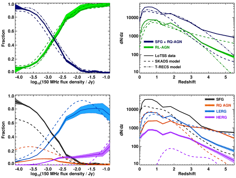
Figure 10: A comparison of the radio source population fractions as a function of 150 MHz flux density (left panels) and the redshift distribution of radio sources (right panels) between the LoTSS-Deep data (solid lines and shaded regions) and the simulated sky predictions from SKADS (Wilman et al., 2008, dashed lines) and T-RECS (Bonaldi et al., 2019, dot-dash lines). The upper panels show the populations split just into star-forming galaxies plus radio quiet AGN (blue) versus radio-loud AGN (green), which can be compared against both SKADS and T-RECS simulations. The lower panels compare the four sub-populations against the SKADS simulation predictions; note that the separation of the two SKADS radio-loud classes does not map precisely onto the HERG/LERG classification used in this paper, although it is reasonably similar (see text).

The upper panels of Figure 10 show the simulation vs data comparison for a simple split into the two T-RECS source populations: star-forming galaxies plus radio-quiet AGN, against radio-loud AGN (HERGs + LERGs). Note that as well as allowing a comparison against both T-RECS and SKADS, this population split is arguably the most robustly determined in the LoTSS-Deep dataset, as it depends only on the presence or absence of a radio-excess rather than the (more difficult to establish) evidence for a radiative AGN. These upper panels show that both T-RECS and SKADS describe fairly well the transition between these two populations with decreasing radio flux density. T-RECS also provides an accurate match to the redshift distribution out to redshift $z\sim 4$, beyond which the simulated source counts fall below those measured in the data; it is not clear whether this is a shortcoming of the simulation, or whether the photometric redshifts of the highest redshift sources become less reliable. The SKADS simulations also match the data reasonably well out to redshift $z\sim 2$, but thereafter they over-predict the number of radio-loud AGN and under-predict the star-forming galaxy population.

The lower panels of Figure 10 provide further analysis of the SKADS simulations, split into the four sub-populations. Here, signficant differences are observed between the simulated and observed datasets. First, SKADS underpredicts the number of SFGs by a factor $\approx 2$ at all redshifts $z\mathrel{\hbox to0.0pt{\lower 3.0pt\hbox{$\mathchar 536\relax$}\hss}\raise 2.0pt\hbox{$\mathchar 318\relax$}}0.2$. This is a result which has previous been established (e.g Bonaldi et al., 2016; Smolčić et al., 2017a); Hale et al. (2023) use a ‘modified SKADS’ model where they double the number of star-forming galaxies. Second, SKADS substantially over-predicts the number of radio-quiet AGN at lower redshifts and lower flux densities compared to the observations. Although it cannot be excluded that this is due to misclassification of faint radio-quiet AGN as star-forming galaxies in the observational data, a more likely explanation is that, as discussed earlier, this is due to an assumed radio spectral index of 0.7 for the radio-quiet AGN; a flatter spectral index (or curved spectral shape due to low-frequency absorption) would lead to a lower prevalence of these sources at the low frequencies of the LoTSS-Deep data. The combination of fewer SFGs and more RQAGN gives rise to the good agreement at low redshifts in the upper panel. For the radio-loud AGN, the difference in the high redshift number counts comes primarily from an over-prediction of the LERG population; the high redshift evolution of these sources was unknown at the time of the SKADS simulations, and so was assumed to be flat beyond $z\sim 0.7$; recent works (e.g Kondapally et al., 2022) show this to be a reasonable assumption out to $z\sim 2$, but with indications of a decline between $2.0<z<2.5$, suggesting a breakdown of the SKADS assumptions.

In conclusion, while the SKADS simulations have been very successful in producing simulated radio skies, datasets such as LoTSS-Deep which probe new parameter space are revealing the shortcomings in our understanding 15 years ago when those simulations were first produced. The more modern T-RECS simulations provide a better match to the current dataset, but would be enhanced by the explicit inclusion of a radio-quiet AGN dataset, since the assumption that the radio emission of these sources is entirely produced through star-formation is known not to be true (see e.g. Macfarlane et al., 2021). Furthermore, explicit separation of the radio-loud population into HERG and LERG components in T-RECS would be a valuable addition and allow more detailed comparison of the simulation performance.

9 Summary

The LoTSS Deep Fields are the widest deep radio survey ever undertaken. The LoTSS-Deep first data release, comprising $\approx$80,000 radio sources, is already an order of magnitude larger than previous radio source samples at this depth. The final LoTSS-Deep sample will detect $>250,000$ radio-selected sources over a 35 deg² region of sky, split into four different fields to largely overcome cosmic variance. Extensive multi-wavelength photometry from the UV to the far-IR in each field facilitates a huge range of scientific exploitation.

In this paper, a combination of four different SED fitting codes has been applied to the multi-wavelength photometry of each of the LoTSS-Deep DR1 sources. Two of the four codes (cigale and agnfitter) include an AGN component in their SED modelling, and these offer an estimate of the AGN contribution to the overall galaxy SED. The other two codes (magphys and bagpipes) do not include AGN components, but offer more comprehensive coverage of the parameter space of the stellar component, and therefore are able to provide more accurate results for galaxies without AGN contributions. By combining the AGN fractional contributions estimated by cigale and agnfitter with the relative fitting ability of these two codes compared against magphys and bagpipes, those galaxies with an AGN contribution to their SED are identified.

Consensus stellar masses and star-formation rates are determined for each galaxy. For the galaxies without AGN contributions, these are generally based on the magphys and bagpipes results, which show excellent overall agreement with each other. For those which do show an AGN contribution to their spectra, the cigale results are primarily adopted, as cigale is shown to provide more reliable estimates than agnfitter.

The consensus star-formation rates are used to determine a relationship between 150 MHz radio luminosity and star-formation rate, using a ‘ridgeline’ approach to minimise bias from both radio selection effects and weak radio-AGN contributions. The determined relation is $\log_{10}L_{\rm 150MHz}=22.24+1.08\log_{10}({\rm SFR})$, where $L_{\rm 150MHz}$ is in units of W Hz^-1 and SFR in units of $M_{\odot}$ yr^-1. This is in very good agreement with previous literature studies. Radio-excess sources are then identified as those sources which show at least 0.7 dex (corresponding to $\approx 3\sigma$) more radio emission than would be expected based on the star formation rate.

Using these results, the LoTSS Deep Field sources are then classified into four classes: (i) star-forming galaxies, which show neither any evidence for an AGN in their optical/IR SED nor a radio-excess; (ii) radio-quiet AGN, which do have an AGN contribution to their optical/IR SED, but show no radio excess; (iii) low-excitation radio galaxies (jet-mode radio-AGN), which show a radio excess but no optical/IR AGN signatures; (iv) high-excitation radio galaxies which show both AGN emission in their optical/IR SED and a radio excess. Less than 5 per cent of the sources are unable to be classified. Overall, over two-thirds of the sources in the LoTSS Deep Fields are star-forming galaxies, around 16 per cent are LERGs, just under 10 per cent are radio-quiet AGN, and 2 per cent are HERGs. The three LoTSS Deep Fields show strong agreement in their source populations, despite significant differences in the input multi-wavelength photometric data.

The star-forming galaxies dominate the population below flux densities of $S_{\rm 150MHz}\approx 1$ mJy, accounting for $\approx$90 per cent of the sources close to the flux limit of the deepest field, $S_{\rm 150MHz}\mathrel{\hbox to0.0pt{\lower 3.0pt\hbox{$\mathchar 536\relax$}\hss}\raise 2.0pt\hbox{$\mathchar 316\relax$}}100\mu$Jy. In terms of luminosity, the star-forming galaxies become the largest population below $L_{\rm 150MHz}\approx 10^{25}$W Hz^-1. At higher flux densities, and higher luminosities, the LERGs are the dominant population. The proportion of HERGs begins to rise significantly at the very highest flux densities and luminosities, but the LoTSS Deep Fields do not cover enough sky area to probe the regime where these become the dominant population.

Star-forming galaxies are observed across all redshifts, ranging from normal star-forming galaxies in the nearby Universe to extreme starbursting systems at $z>4$. They are also observed across a wide range of optical magnitudes and stellar masses, peaking at around $10^{10.5}$ solar masses, typical of galaxies towards the upper end of the star-forming main sequence. The proportion of radio-quiet AGN rises noticeably towards higher redshifts; it also rises sharply towards the highest stellar masses, but this is likely to be an artefact of the steep stellar mass function coupled with larger uncertainties on the stellar masses of this population. The LERG population reaches its peak importance at redshifts 1 to 3; however, the proportion of LERGs is smaller than that of the star-forming galaxies at all redshifts, stellar masses and optical magnitudes.

The observed populations are compared against the prediction of the SKADS and T-RECS radio sky simulations. SKADS is shown to underpredict the star-forming galaxy population by a factor $\approx 2$ across all redshifts. It over-predicts the proportion of radio-quiet AGN in the sample. This is likely to be due to the assumption of a radio spectral index of $\alpha=0.7$ for these sources: a flatter spectral index, as indicated by recent LOFAR observations of radio-quiet quasars, would reduce the prevalence of these sources in these low-frequency observations. Finally, SKADS over-predicts the numbers of LERGs at redshifts $z>2$, as it does not account for the negative cosmic evolution of this population at high redshift beginning to be observed in the latest datasets. T-RECS provides a good match to the star-forming and radio-loud AGN populations, but its lack of a separate radio-quiet AGN population is a significant shortcoming.

The classifications, stellar masses and SFRs derived in this paper form a vital input to many other studies using the LoTSS Deep Fields first data release (Smith et al., 2021; Bonato et al., 2021; Kondapally et al., 2022; McCheyne et al., 2022; Mingo et al., 2022; Cochrane et al., 2023, and others), and the techniques developed to derive these can be applied to future data releases of the LoTSS Deep Fields. Many advances continue to be made in the LoTSS Deep Fields that, in addition to new deeper radio data, will improve classifications still further. Over the next 5 years, the WEAVE-LOFAR survey (Smith et al., 2016) will obtain around a million optical spectra of LOFAR sources, including all sources detected in the LoTSS Deep Fields, using the new William Herschel Telescope (WHT) Enhanced Area Velocity Explorer (WEAVE) multi-object spectrograph (Jin et al., 2023). WEAVE-LOFAR will provide spectroscopic redshifts for the vast majority of the star-forming galaxies, radio-quiet AGN and HERGs (especially at lower redshifts) due to their strong emission lines, removing one of the largest uncertainties in the SED fitting. It may be possible to obtain spectroscopic redshifts for LERGs from weaker lines or continuum features, and even where this is not the case, the confirmed absence of strong emission lines and AGN features will add confidence to the reliability of the photometric redshifts. For many sources, WEAVE-LOFAR will also improve source classifications through either emission line diagnostics, or emission line to radio flux ratios (cf. Best & Heckman, 2012, at lower redshifts). Future imaging of these fields at 0.3-arcsec resolution, by including the international LOFAR baselines (cf. Morabito et al., 2022; Sweijen et al., 2022), will further improve source classification by allowing compact radio cores (AGN), kpc-scale star-forming regions, and small-scale core-jet radio sources to be distinguished by their radio morphology in these fields (Morabito et al., 2022). A comparison between the SED-determined classifications and those from high resolution radio morphology will be very interesting.

The final LoTSS-Deep sample, imaged with sub-arcsec radio resolution and coupled with high-resolution optical spectroscopy for each source, will represent an extremely powerful resource for studies of the evolution of galaxies and AGN.

Data Availability

The data used in this paper come from the LoTSS Deep Fields Data Release 1. The radio images and radio catalogues are presented by Tasse et al. (2021) and Sabater et al. (2021), and were made publicly available through both the Centre de Données astronomiques de Strasbourg (CDS) and through the LOFAR Surveys website at https://lofar-surveys.org/deepfields.html. The multi-wavelength photometric catalogues and photometric redshifts come from Kondapally et al. (2021) and Duncan et al. (2021) respectively, both of which are also available through CDS and the LOFAR Surveys website. For each field, a table of classifications, stellar masses and SFRs is made available electronically as part of this paper. Furthermore, the adapted input photometric catalogue developed in Sec. 3.3 for the SED fitting, and a table of the key SED fitting results from Secs. 4, 5 and 6 have been made available on https://lofar-surveys.org/deepfields.html. More extensive SED fitting results from each code can be made available upon reasonable request to the corresponding author.

Appendix A Uncertainties on stellar masses and SFRs

As discussed in the main text, no attempt is made to derive stellar mass or SFR uncertainties on a source-by-source basis: any reader interested in individual sources can examine the results of all of the different SED codes, provided in the extended tables on the lofar-surveys.org website, and make their own assessment of the relevant systematic and statistical errors. Instead, this appendix examines typical uncertainties that can broadly be considered.

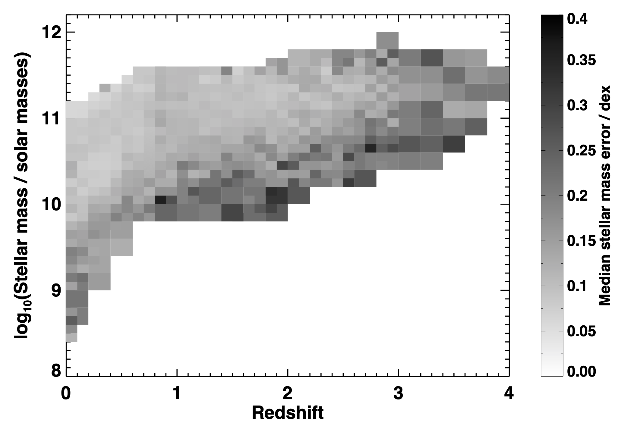
Figure 11: Typical uncertainties on estimates of stellar mass, as a function of both stellar mass and redshift, for non-AGN in the ELAIS-N1 field. At lower redshifts and higher stellar masses, the uncertainty is generally $\sim 0.1$dex, but this increases towards lower stellar masses and for redshifts $z>2$.

For sources not identified as radiative-mode AGN, the consensus stellar masses are derived using the magphys and bagpipes results. For each source, the difference between the outputs of the two codes provides an indication of systematic uncertainties, while the confidence intervals provided by each code give an estimate of statistical uncertainty. As a broad guide to the dominant uncertainty, for each source the higher of these two values is considered. Figure 11 then shows the median of this value for all galaxies within a given bin in redshift–mass space. As can be seen, the calculated median uncertainties are typically $\mathrel{\hbox to0.0pt{\lower 3.0pt\hbox{$\mathchar 536\relax$}\hss}\raise 2.0pt\hbox{$\mathchar 316\relax$}}0.1$ dex at lower redshifts and higher masses. As expected, they increase towards lower masses and towards higher redshifts, in both cases due to the galaxies being fainter and therefore having lower signal-to-noise photometric measurements in the SED fitting.

The uncertainties in Fig. 11 can broadly be categorised in four different ranges of parameter space, with empirical estimates of the uncertainty possible for each:

• Higher mass, lower redshift: specifically $\log_{10}M_{*}\geq(9.7+2.5\log_{10}(1+z))$ and $z\leq 2$. Here the uncertainty on stellar mass is fairly constant at $\Delta M_{*}\approx 0.1$ dex.

• Higher mass, higher redshift: specifically $\log_{10}M_{*}\geq(9.7+2.5\log_{10}(1+z))$ and $z>2$. Here the uncertainty increases with increasing redshift and can be approximated as $\Delta M_{*}\approx 0.05z$ dex.

• Lower mass, lower redshift: specifically $\log_{10}M_{*}<(9.7+2.5\log_{10}(1+z))$ and $z\leq 2$. Here the uncertainty increases with decreasing mass and increasing redshift, broadly as $\Delta M_{*}\approx 0.1+0.08(1+z)(9.7+2.5\log_{10}(1+z)-\log_{10}M_{*})$ dex.

• Lower mass, higher redshift: specifically $\log_{10}M_{*}<(9.7+2.5\log_{10}(1+z))$ and $z>2$. The relative high uncertainties here match on to the lower redshift and higher mass regimes: $\Delta M_{*}\approx 0.05z+0.24(9.7+2.5\log_{10}(1+z)-\log_{10}M_{*})$ dex.

Uncertainties on the stellar masses of the radiative AGN are harder to estimate in this manner, as mass estimates are derived from the two cigale fits, and these are likely to be subject to related systematic errors. Comparing the confidence intervals of the cigale fits with those of the non-AGN in the same redshift-mass bin, the statistical uncertainties of the radiative-mode AGN are on average 20 per cent larger than those of the non-AGN; this sets a lower limit to the mass uncertainty estimate, although it is likely that the systematic errors will also be larger in cases where the AGN contributes significantly to the optical to near-IR spectrum.

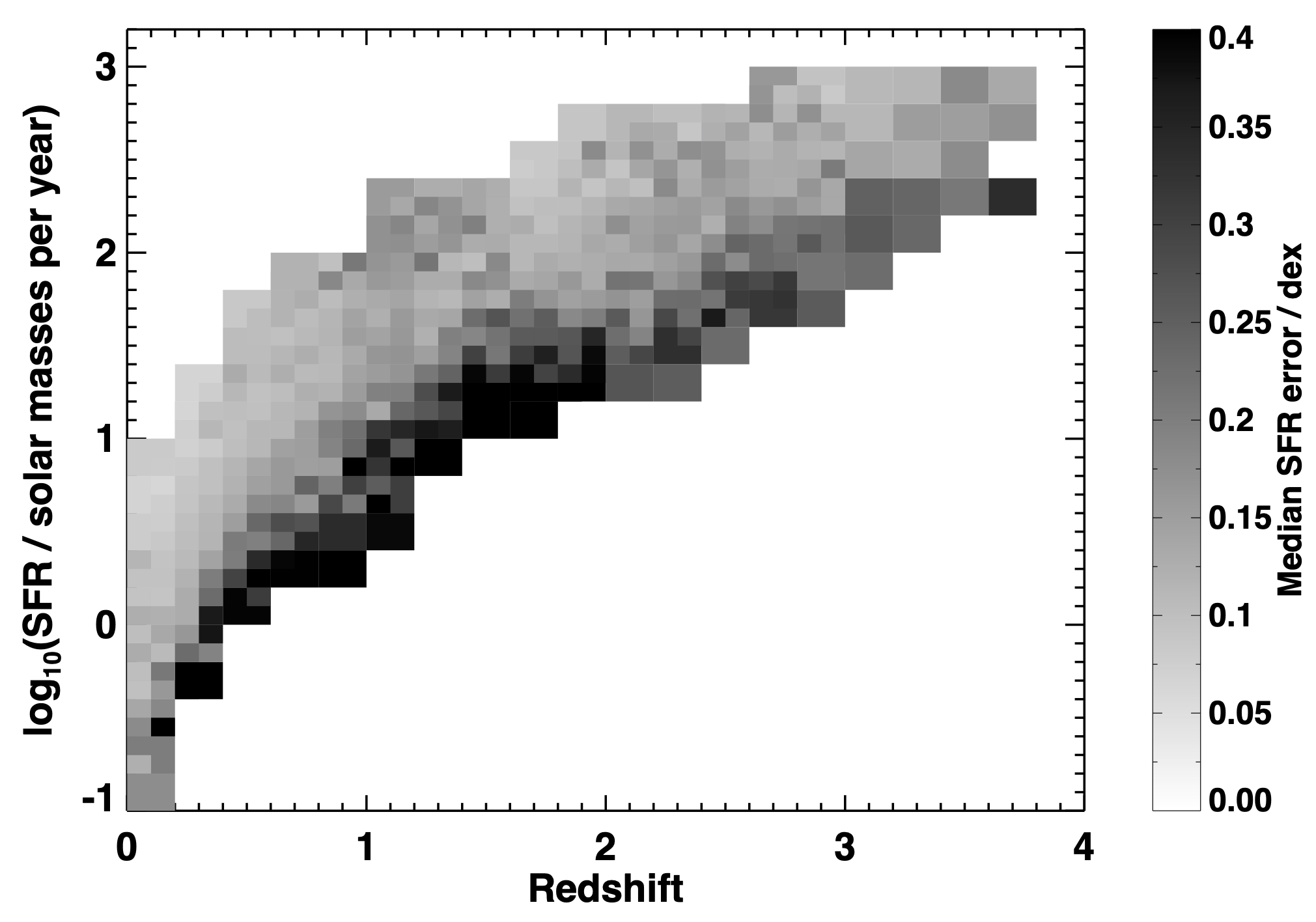
Figure 12: Typical uncertainties on estimates of SFR, as a function of both SFR and redshift, for non-AGN in the ELAIS-N1 field. SFR uncertainties increase dramatically for the few per cent of sources at the lowest SFRs at each redshift; above that they have little dependence on SFR, but increase gradually with increasing redshift.

A similar approach can be followed to estimate the typical uncertainties on the consensus SFR estimates. Fig. 12 shows the result, split into bins of SFR and redshift. In this case it is apparent that the SFR estimates are generally robust until the very lowest SFRs at any redshift are reached (at most a few per cent of objects), where the uncertainties increase dramatically. For the vast majority of the population at higher SFRs, there is no strong dependence of the SFR uncertainty (in dex) on the measured SFR, but a clear trend for the uncertainty to increase with redshift, from $\approx 0.1$ dex at $z\sim 0$ up to 0.15 dex by $z\sim 1$ and 0.2 dex by $z=3$. This can be empirically approximated as $\Delta$(SFR) $\approx 0.1\times(1+z)^{0.5}$ dex. The contributions to this uncertainty from differences between codes and from the statistical uncertainties within individual codes are comparable in size.

It should be emphasized again that these empirical relations are only intended to provide a guide to the approximate stellar mass and SFR uncertainties, and do not represent reliable values on a source-by-source basis.

References

- Aihara et al. (2018) Aihara H., et al., 2018, PASJ, 70, S8
- An et al. (2023) An F., et al., 2023, MNRAS, submitted; arXiv:2303.06941
- Ashby et al. (2009) Ashby M. L. N., et al., 2009, ApJ, 701, 428
- Asplund et al. (2009) Asplund M., Grevesse N., Sauval A. J., Scott P., 2009, ARA&A, 47, 481
- Baldwin et al. (1981) Baldwin J. A., Phillips M. M., Terlevich R., 1981, PASP, 93, 5
- Becker et al. (1995) Becker R. H., White R. L., Helfand D. J., 1995, ApJ, 450, 559
- Best & Heckman (2012) Best P. N., Heckman T. M., 2012, MNRAS, 421, 1569
- Best et al. (2005) Best P. N., et al., 2005, MNRAS, 362, 25
- Best et al. (2014) Best P. N., Ker L. M., Simpson C., Rigby E. E., Sabater J., 2014, MNRAS, 445, 955
- Bian et al. (2013) Bian F., et al., 2013, ApJ, 774, 28
- Bonaldi et al. (2016) Bonaldi A., Harrison I., Camera S., Brown M. L., 2016, MNRAS, 463, 3686
- Bonaldi et al. (2019) Bonaldi A., Bonato M., Galluzzi V., Harrison I., Massardi M., Kay S., De Zotti G., Brown M. L., 2019, MNRAS, 482, 2
- Bonato et al. (2021) Bonato M., et al., 2021, A&A, 656, A48
- Bondi et al. (2023) Bondi M., et al., 2023, in preparation
- Boquien et al. (2019) Boquien M., Burgarella D., Roehlly Y., Buat V., Ciesla L., Corre D., Inoue A. K., Salas H., 2019, A&A, 622, A103
- Botteon et al. (2022) Botteon A., et al., 2022, Science Advances, 8, eabq7623
- Brienza et al. (2017) Brienza M., et al., 2017, A&A, 606, A98
- Brown et al. (2007) Brown M. J. I., Dey A., Jannuzi B. T., Brand K., Benson A. J., Brodwin M., Croton D. J., Eisenhardt P. R., 2007, ApJ, 654, 858
- Brown et al. (2008) Brown M. J. I., et al., 2008, ApJ, 682, 937
- Brown et al. (2014) Brown M. J. I., et al., 2014, ApJS, 212, 18
- Brown et al. (2017) Brown M. J. I., et al., 2017, ApJ, 847, 136
- Brown et al. (2019) Brown M. J. I., Duncan K. J., Landt H., Kirk M., Ricci C., Kamraj N., Salvato M., Ananna T., 2019, MNRAS, 489, 3351
- Bruzual & Charlot (2003) Bruzual G., Charlot S., 2003, MNRAS, 344, 1000
- Buat et al. (2019) Buat V., Ciesla L., Boquien M., Małek K., Burgarella D., 2019, A&A, 632, A79
- Burgarella et al. (2005) Burgarella D., Buat V., Iglesias-Páramo J., 2005, MNRAS, 360, 1413
- Byler et al. (2017) Byler N., Dalcanton J. J., Conroy C., Johnson B. D., 2017, ApJ, 840, 44
- Calistro Rivera et al. (2016) Calistro Rivera G., Lusso E., Hennawi J. F., Hogg D. W., 2016, ApJ, 833, 98
- Calistro Rivera et al. (2017) Calistro Rivera G., et al., 2017, MNRAS, 469, 3468
- Calzetti et al. (2000) Calzetti D., Armus L., Bohlin R. C., Kinney A. L., Koornneef J., Storchi-Bergmann T., 2000, ApJ, 533, 682
- Carnall et al. (2018) Carnall A. C., McLure R. J., Dunlop J. S., Davé R., 2018, MNRAS, 480, 4379
- Carnall et al. (2019) Carnall A. C., Leja J., Johnson B. D., McLure R. J., Dunlop J. S., Conroy C., 2019, ApJ, 873, 44
- Chabrier (2003) Chabrier G., 2003, PASP, 115, 763
- Chambers et al. (2016) Chambers K. C., et al., 2016, arXiv e-prints, p. arXiv:1612.05560
- Charlot & Fall (2000) Charlot S., Fall S. M., 2000, ApJ, 539, 718
- Cochrane et al. (2021) Cochrane R. K., et al., 2021, MNRAS, 503, 2622
- Cochrane et al. (2023) Cochrane R. K., et al., 2023, MNRAS, submitted
- Condon (1992) Condon J. J., 1992, ARA&A, 30, 575
- Condon et al. (1998) Condon J. J., Cotton W. D., Greisen E. W., Yin Q. F., Perley R. A., Taylor G. B., Broderick J. J., 1998, AJ, 115, 1693
- Condon et al. (2002) Condon J. J., Cotton W. D., Broderick J. J., 2002, AJ, 124, 675
- Cool (2007) Cool R. J., 2007, ApJS, 169, 21
- Delhaize et al. (2017) Delhaize J., et al., 2017, A&A, 602, A4
- Delvecchio et al. (2017) Delvecchio I., et al., 2017, A&A, 602, A3
- Donley et al. (2012) Donley J. L., et al., 2012, ApJ, 748, 142
- Draine & Li (2007) Draine B. T., Li A., 2007, ApJ, 657, 810
- Draine et al. (2014) Draine B. T., et al., 2014, ApJ, 780, 172
- Duncan et al. (2019) Duncan K. J., et al., 2019, A&A, 622, A3
- Duncan et al. (2021) Duncan K. J., et al., 2021, A&A, 648, A4
- Dunlop et al. (2017) Dunlop J. S., et al., 2017, MNRAS, 466, 861
- Fabian (2012) Fabian A. C., 2012, ARA&A, 50, 455
- Fanaroff & Riley (1974) Fanaroff B. L., Riley J. M., 1974, MNRAS, 167, 31P
- Ferland et al. (2017) Ferland G. J., et al., 2017, Rev. Mex. Astron. Astrofis., 53, 385
- Fitzpatrick (1999) Fitzpatrick E. L., 1999, PASP, 111, 63
- Fomalont et al. (2006) Fomalont E. B., Kellermann K. I., Cowie L. L., Capak P., Barger A. J., Partridge R. B., Windhorst R. A., Richards E. A., 2006, ApJS, 167, 103
- Fritz et al. (2006) Fritz J., Franceschini A., Hatziminaoglou E., 2006, MNRAS, 366, 767
- Gao et al. (2021) Gao F., et al., 2021, A&A, 654, A117
- Gloudemans et al. (2021) Gloudemans A. J., et al., 2021, A&A, 656, A137
- Gonzalez et al. (2010) Gonzalez A. H., et al., 2010, in American Astronomical Society Meeting Abstracts #216. p. 415.13
- Gürkan et al. (2014) Gürkan G., Hardcastle M. J., Jarvis M. J., 2014, MNRAS, 438, 1149
- Gürkan et al. (2018) Gürkan G., et al., 2018, MNRAS, 475, 3010
- Gürkan et al. (2019) Gürkan G., et al., 2019, A&A, 622, A11
- Hale et al. (2021) Hale C. L., et al., 2021, Publ. Astron. Soc. Australia, 38, e058
- Hale et al. (2023) Hale C. L., et al., 2023, MNRAS, 520, 2668
- Hardcastle & Croston (2020) Hardcastle M. J., Croston J. H., 2020, New Astron. Rev., 88, 101539
- Harrison et al. (2016) Harrison I., Camera S., Zuntz J., Brown M. L., 2016, MNRAS, 463, 3674
- Hayward & Smith (2015) Hayward C. C., Smith D. J. B., 2015, MNRAS, 446, 1512
- Heckman & Best (2014) Heckman T. M., Best P. N., 2014, ARA&A, 52, 589
- Heywood et al. (2021) Heywood I., et al., 2021, ApJ, 910, 105
- Heywood et al. (2022) Heywood I., et al., 2022, MNRAS, 509, 2150
- Hildebrandt et al. (2016) Hildebrandt H., et al., 2016, MNRAS, 463, 635
- Hodge et al. (2011) Hodge J. A., Becker R. H., White R. L., Richards G. T., Zeimann G. R., 2011, AJ, 142, 3
- Hurley-Walker et al. (2022) Hurley-Walker N., et al., 2022, Publ. Astron. Soc. Australia, 39, e035
- Hurley et al. (2017) Hurley P. D., et al., 2017, MNRAS, 464, 885
- Intema et al. (2017) Intema H. T., Jagannathan P., Mooley K. P., Frail D. A., 2017, A&A, 598, A78
- Jannuzi & Dey (1999) Jannuzi B. T., Dey A., 1999, in Weymann R., Storrie-Lombardi L., Sawicki M., Brunner R., eds, Astronomical Society of the Pacific Conference Series Vol. 191, Photometric Redshifts and the Detection of High Redshift Galaxies. p. 111
- Jarvis et al. (2019) Jarvis M. E., et al., 2019, MNRAS, 485, 2710
- Jelić et al. (2014) Jelić V., et al., 2014, A&A, 568, A101
- Jin et al. (2023) Jin S., et al., 2023, MNRAS,
- Jurlin et al. (2020) Jurlin N., et al., 2020, A&A, 638, A34
- Kennicutt (1998) Kennicutt Jr. R. C., 1998, ApJ, 498, 541
- Kochanek et al. (2012) Kochanek C. S., et al., 2012, ApJS, 200, 8
- Kondapally et al. (2021) Kondapally R., et al., 2021, A&A, 648, A3
- Kondapally et al. (2022) Kondapally R., et al., 2022, MNRAS, 513, 3742
- Kormendy & Ho (2013) Kormendy J., Ho L. C., 2013, ARA&A, 51, 511
- Krolik & Begelman (1988) Krolik J. H., Begelman M. C., 1988, ApJ, 329, 702
- Lacy et al. (2004) Lacy M., et al., 2004, ApJS, 154, 166
- Lacy et al. (2020) Lacy M., et al., 2020, PASP, 132, 035001
- Lawrence et al. (2007) Lawrence A., et al., 2007, MNRAS, 379, 1599
- Leja et al. (2018) Leja J., Johnson B. D., Conroy C., van Dokkum P., 2018, ApJ, 854, 62
- Lockman et al. (1986) Lockman F. J., Jahoda K., McCammon D., 1986, ApJ, 302, 432
- Lonsdale et al. (2003) Lonsdale C. J., et al., 2003, PASP, 115, 897
- Macfarlane et al. (2021) Macfarlane C., et al., 2021, MNRAS, 506, 5888
- Madau & Dickinson (2014) Madau P., Dickinson M., 2014, ARA&A, 52, 415
- Mahony et al. (2016) Mahony E. K., et al., 2016, MNRAS, 463, 2997
- Małek et al. (2018) Małek K., et al., 2018, A&A, 620, A50
- Małek et al. (2023) Małek K., et al., 2023, in preparation
- Martin et al. (2005) Martin D. C., et al., 2005, ApJ, 619, L1
- Masini et al. (2020) Masini A., et al., 2020, ApJS, 251, 2
- Mauch et al. (2003) Mauch T., Murphy T., Buttery H. J., Curran J., Hunstead R. W., Piestrzynski B., Robertson J. G., Sadler E. M., 2003, MNRAS, 342, 1117
- Mauduit et al. (2012) Mauduit J. C., et al., 2012, PASP, 124, 714
- McCheyne et al. (2022) McCheyne I., et al., 2022, A&A, 662, A100
- McNamara & Nulsen (2007) McNamara B. R., Nulsen P. E. J., 2007, ARA&A, 45, 117
- McPartland et al. (2023) McPartland C., et al., 2023, in preparation
- Messias et al. (2012) Messias H., Afonso J., Salvato M., Mobasher B., Hopkins A. M., 2012, ApJ, 754, 120
- Mingo et al. (2022) Mingo B., et al., 2022, MNRAS, 511, 3250
- Morabito et al. (2022) Morabito L. K., et al., 2022, A&A, 658, A1
- Morganti et al. (2021) Morganti R., et al., 2021, A&A, 648, A9
- Muzzin et al. (2009) Muzzin A., et al., 2009, ApJ, 698, 1934
- Narayan & Yi (1994) Narayan R., Yi I., 1994, ApJ, 428, L13
- Narayan & Yi (1995) Narayan R., Yi I., 1995, ApJ, 452, 710
- Noll et al. (2009) Noll S., Burgarella D., Giovannoli E., Buat V., Marcillac D., Muñoz-Mateos J. C., 2009, A&A, 507, 1793
- Norris et al. (2011) Norris R. P., et al., 2011, Publ. Astron. Soc. Australia, 28, 215
- Norris et al. (2013) Norris R. P., et al., 2013, Publ. Astron. Soc. Australia, 30, e020
- Novak et al. (2017) Novak M., et al., 2017, A&A, 602, A5
- Oliver et al. (2000) Oliver S., et al., 2000, MNRAS, 316, 749
- Oliver et al. (2012) Oliver S. J., et al., 2012, MNRAS, 424, 1614
- Owen (2018) Owen F. N., 2018, ApJS, 235, 34
- Owen & Morrison (2008) Owen F. N., Morrison G. E., 2008, AJ, 136, 1889
- Pacifici et al. (2023) Pacifici C., et al., 2023, ApJ, 944, 141
- Padovani (2016) Padovani P., 2016, A&ARv, 24, 13
- Pearson et al. (2018) Pearson W. J., et al., 2018, A&A, 615, A146
- Pracy et al. (2016) Pracy M. B., et al., 2016, MNRAS, 460, 2
- Prandoni et al. (2018) Prandoni I., Guglielmino G., Morganti R., Vaccari M., Maini A., Röttgering H. J. A., Jarvis M. J., Garrett M. A., 2018, MNRAS, 481, 4548
- Raccanelli et al. (2012) Raccanelli A., et al., 2012, MNRAS, 424, 801
- Rengelink et al. (1997) Rengelink R. B., Tang Y., de Bruyn A. G., Miley G. K., Bremer M. N., Roettgering H. J. A., Bremer M. A. R., 1997, A&AS, 124, 259
- Sabater et al. (2019) Sabater J., et al., 2019, A&A, 622, A17
- Sabater et al. (2021) Sabater J., et al., 2021, A&A, 648, A2
- Schinnerer et al. (2007) Schinnerer E., et al., 2007, ApJS, 172, 46
- Schlegel et al. (1998) Schlegel D. J., Finkbeiner D. P., Davis M., 1998, ApJ, 500, 525
- Schober et al. (2017) Schober J., Schleicher D. R. G., Klessen R. S., 2017, MNRAS, 468, 946
- Scudder et al. (2016) Scudder J. M., Oliver S., Hurley P. D., Griffin M., Sargent M. T., Scott D., Wang L., Wardlow J. L., 2016, MNRAS, 460, 1119
- Shakura & Sunyaev (1973) Shakura N. I., Sunyaev R. A., 1973, A&A, 500, 33
- Shimwell et al. (2017) Shimwell T. W., et al., 2017, A&A, 598, A104
- Shimwell et al. (2019) Shimwell T. W., et al., 2019, A&A, 622, A1
- Shimwell et al. (2022) Shimwell T. W., et al., 2022, A&A, 659, A1
- Shirley et al. (2021) Shirley R., et al., 2021, MNRAS, 507, 129
- Siewert et al. (2020) Siewert T. M., et al., 2020, A&A, 643, A100
- Simpson et al. (2006) Simpson C., et al., 2006, MNRAS, 372, 741
- Smith et al. (2012) Smith D. J. B., et al., 2012, MNRAS, 427, 703
- Smith et al. (2016) Smith D. J. B., et al., 2016, in Reylé C., Richard J., Cambrésy L., Deleuil M., Pécontal E., Tresse L., Vauglin I., eds, SF2A-2016: Proceedings of the Annual meeting of the French Society of Astronomy and Astrophysics. pp 271–280 (arXiv:1611.02706)
- Smith et al. (2021) Smith D. J. B., et al., 2021, A&A, 648, A6
- Smolčić et al. (2017a) Smolčić V., et al., 2017a, A&A, 602, A1
- Smolčić et al. (2017b) Smolčić V., et al., 2017b, A&A, 602, A2
- Smolčić et al. (2017c) Smolčić V., et al., 2017c, A&A, 602, A6
- Smolčić et al. (2018) Smolčić V., et al., 2018, A&A, 620, A14
- Stalevski et al. (2012) Stalevski M., Fritz J., Baes M., Nakos T., Popović L. Č., 2012, MNRAS, 420, 2756
- Stalevski et al. (2016) Stalevski M., Ricci C., Ueda Y., Lira P., Fritz J., Baes M., 2016, MNRAS, 458, 2288
- Stern et al. (2005) Stern D., et al., 2005, ApJ, 631, 163
- Sweijen et al. (2022) Sweijen F., et al., 2022, Nature Astronomy, 6, 350
- Symeonidis & Page (2021) Symeonidis M., Page M. J., 2021, MNRAS, 503, 3992
- Tasse et al. (2021) Tasse C., et al., 2021, A&A, 648, A1
- Wang et al. (2019) Wang L., et al., 2019, A&A, 631, A109
- Wang et al. (2021) Wang L., et al., 2021, A&A, 648, A8
- Wayth et al. (2015) Wayth R. B., et al., 2015, Publ. Astron. Soc. Australia, 32, e025
- Whittam et al. (2022) Whittam I. H., et al., 2022, MNRAS, 516, 245
- Williams et al. (2018) Williams W. L., et al., 2018, MNRAS, 475, 3429
- Williams et al. (2019) Williams W. L., et al., 2019, A&A, 622, A2
- Wilman et al. (2008) Wilman R. J., et al., 2008, MNRAS, 388, 1335
- Wright et al. (2010) Wright E. L., et al., 2010, AJ, 140, 1868
- Yang et al. (2020) Yang G., et al., 2020, MNRAS, 491, 740
- da Cunha et al. (2008) da Cunha E., Charlot S., Elbaz D., 2008, MNRAS, 388, 1595
- van Haarlem et al. (2013) van Haarlem M. P., et al., 2013, A&A, 556, A2