Deep Learning of Sea Surface Temperature Patterns to Identify Ocean Extremes

Abstract

We perform an out-of-distribution (OOD) analysis of $\sim$12,000,000 semi-independent 128x128 pixel² sea surface temperature (SST) regions, which we define as cutouts, from all nighttime granules in the MODIS R2019 Level-2 public dataset to discover the most complex or extreme phenomena at the ocean surface. Our algorithm (ulmo) is a probabilistic autoencoder (PAE), which combines two deep learning modules: (1) an autoencoder, trained on $\sim$150,000 random cutouts from 2010, to represent any input cutout with a 512-dimensional latent vector akin to a (non-linear) Empirical Orthogonal Function (EOF) analysis; and (2) a normalizing flow, which maps the autoencoder’s latent space distribution onto an isotropic Gaussian manifold. From the latter, we calculate a log-likelihood (LL) value for each cutout and define outlier cutouts  to be those in the lowest 0.1% of the distribution. These exhibit large gradients and patterns characteristic of a highly dynamic ocean surface, and many are located within larger complexes whose unique dynamics warrant future analysis. Without guidance, ulmo consistently locates the outliers where the major western boundary currents separate from the continental margin. Buoyed by these results, we begin the process of exploring the fundamental patterns learned by ulmo  identifying several compelling examples. Future work may find that algorithms like ulmo hold significant potential/promise to learn and derive other, not-yet-identified behaviors in the ocean from the many archives of satellite-derived SST fields. As important, we see no impediment to applying them to other large, remote-sensing datasets for ocean science (e.g., SSH, ocean color).

1 Introduction

Satellite-borne sensors have for many years, been collecting data used to estimate a broad range of meteorological, oceanographic, terrestrial and cryospheric properties. Of significance with regard to the fields associated with these properties is their global coverage and relatively high spatial (meters to tens of kilometers) and temporal (hours to tens of days) resolutions. These datasets tend to be very large, well documented and readily accessible making them ideal targets for analyses using modern machine learning techniques. Based on our knowledge of, interest in and access to global SST datasets, we have chosen one of these to explore the possibilities. Specifically, inspired by the question of “what lurks within” and also the desire to identify complex and/or extreme phenomena of the upper ocean, we have developed an unsupervised machine learning algorithm named ulmo to analyze the nighttime MODerate-resolution Imaging Spectroradiometer (MODIS) Level-2 (L2) SST dataset obtained from the National Aeronautics and Space Administration (NASA) spacecraft, Aqua, spanning years 2003-2019. The former (the unknown unknowns) could reveal previously unanticipated physical processes at or near the ocean’s surface. Such surprises are, by definition, rare and require massive datasets and semi-automated approaches to examine them. The latter type (extrema) affords an exploration of the incidence and spatial distribution of complex phenomena across the entire ocean. Similar ‘fishing’ expeditions have been performed in other fields on large imaging datasets (e.g., astronomy Abul Hayat et al., 2020). However, to our knowledge, this is the first application of machine learning for open-ended exploration of a large oceanographic dataset, although there is a rapidly growing body of literature on applying machine learning techniques to the specifics of SST retrieval algorithms Saux Picart et al. (2018), cloud detection Paul & Huntemann (2020), eddy location Moschos et al. (2020), prediction Ratnam et al. (2020); Zhang et al. (2020); Yu et al. (2020), etc. and, more generally, to remote sensing Ma et al. (2019).

Previous analyses of SST on local or global scales have emphasized standard statistics (e.g., mean and RMS) and/or linear methods for pattern assessment (e.g., FFT and EOF). While these metrics and techniques offer fundamental measures of the SST fields, they may not fully capture the complexity inherent in the most dynamic regions of the ocean. Motivated by advances in the analysis of natural images in computer vision, we employ a PAE which utilizes a Convolutional Neural Network (CNN) to learn the diversity of SST patterns. By design, the CNN learns the features most salient to the dataset, with built-in methodology to examine the image on a wide range of scales. Further, its non-linearity and invariance to translation offer additional advantages over EOF and like applications.

The ulmo algorithm is a PAE, a deep learning tool designed for density estimation. By combining an autoencoder with a normalizing flow, the PAE is able to approximate the likelihood function for arbitrary data while also avoiding a common downfall of flow models: their sensitivity to noisy or otherwise uninformative background features in the input Nalisnick et al. (2018). By first reducing our raw data (an SST field) to a compact set of the most pertinent learned features via the non-linear compression of an autoencoder, the PAE then provides an estimate of its probability by transforming the latent vector into a sample from an equal-dimension isotropic Gaussian distribution where computing the probability is trivial. We can then select the lowest probability fields as outliers or anomalous.

Our secondary goal of this manuscript, is to pioneer the process for like studies on other large earth science datasets in general and oceanographic datasets in particular including those associated with the output of numerical models. A similar analysis of SST fields output by ocean circulation models is of particular interest as an adjunct to the work presented herein. As will become clear, we understand some of the segmentation suggested by ulmo by not all of it. The method has also identified some anomalous events for which the basics physics is not clear. Assuming that the analysis of model-derived SST fields yields similar results, the additional output available from the model, the vector velocity field and salinity, as well as a time series of fields, will allow for a dynamic investigation of the processes involved.

This manuscript is organized as follows: Section 2 describes the data analyzed here, Section 3 details the methodology, Section 4 presents the primary results, and Section 5 provides a brief set of conclusions. All of the software and final data products generated by this study are made available on-line https://github.com/AI-for-Ocean-Science/ulmo.

2 Data

With a primary goal to identify regions of the ocean exhibiting rare yet physical phenomena, we chose to focus on the L2 SST Aqua MODIS dataset (https://oceancolor.gsfc.nasa.gov/data/aqua/). The associated five minute segments, each covering $\approx 2000\times 1350$ km of the Earth’s surface and referred to as granules, have $\approx 1$ km spatial resolution and span the entire ocean, clouds permitting, twice daily. For this study, we examined all nighttime granules from 2003-2019. The SST fields, the primary element of these granules, were processed by the Ocean Biology Processing Group (OBPG) at NASA’s Goddard Space Flight Center, Ocean Ecology Laboratory from the MODIS radiometric data using the R2019 retrieval algorithm Minnett et al. (1-4 June 2020) and were uploaded from the OBPG’s public server (https://oceancolor.gsfc.nasa.gov/cgi/browse.pl?sen=amod) to the University of Rhode Island (URI).

The method developed here requires a set of same-sized images. When exploring complex physical phenomena in the ocean, one is often interested in one of two spatial scales determined by the relative importance of rotation to inertia in the associated processes. The separation between these scales is generally taken to be the Rossby Radius of deformation, $R_{o}$, which, at mid-latitude is $\sim\mathcal{O}(30)$ km. Processes with scales larger than $R_{o}$ are referred to as mesoscale processes for which the importance of rotation dominates. At smaller scales the processes are referred to as sub-mesoscale. For this study, we chose to focus on the former and extracted $128\times 128$ pixel images, which we refer to as cutouts, from the MODIS granules. Cutouts are approximately 128 km on a side. We are confident, supported by limited experimentation, that the techniques described here will apply to other scales as well.

The analysis was further restricted to data within 480 pixels of nadir. This constraint was added to reduce the influence of pixel size on the selection process for outliers; the along-scan size of pixels increases away from nadir as does the rate of this increase. To distances of $\sim$480 km the change in along-scan pixel size is less than a factor of two; at the edge of the swath the along-scan pixel size is approximately $\sim 5$ times that at nadir.

The L2 MODIS product includes a quality flag – a measure of confidence of the retrieved SST – with values from 0 (best) to 4 (value not retrieved). The primary reason for assigning a poor quality to a pixel is due to cloud contamination although there are other issues that result in a poor quality rating Kilpatrick et al. (2019). A quality threshold of 2 was used for this study. Because the incidence, sizes, and shapes of clouds are highly variable (both temporally and spatially), an OOD algorithm trained on images with some cloud contamination may become more sensitive to cloud patterns than unusual SST patterns. Indeed, our initial experiments were stymied by clouds with the majority of outlier cutouts showing unusual cloud patterns, suggesting an application of this approach to the study of clouds as well. To mitigate this effect, we further restricted the dataset to cutouts with very low cloud cover (CC), defined as the fraction of the cutout image masked for clouds or other image defects. After experimenting with model performance for various choices of CC, we settled on a conservative limit of ${\rm\acs{CC}}\leq 5\%$ as a compromise between dataset size and our ability to further mitigate clouds (and other masked pixels) with an inpainting algorithm (see next section).

From each granule, we extracted a set of 128x128 cutouts satisfying ${\rm\acs{CC}}\leq 5\%$ and distance to nadir of the central pixel $\leq$480 km. To well-sample the granule while limiting the number of highly overlapping cutouts, we drew at most one cutout from a pre-defined 32x32 pixel grid on the granule. This procedure yields $\approx 700,000$ cutouts per year and 12,358,049 cutouts for the full analysis.

Of course, by requiring regions largely free of clouds (${\rm\acs{CC}}<5\%$), we are significantly restricting the dataset and undoubtedly biasing the regions of ocean analyzed both in time and space. Figure 1 shows the spatial distribution of the full dataset across the ocean. The coastal regions show the highest incidence of multiple observations, but nearly all of the ocean was covered by one or more cutouts. Given this spatial distribution, one might naively expect the results to be biased against coastal regions because these were sampled at higher frequency and comprises a greater fraction of the full distribution. This is mitigated, in part, by the fact that the non-coastal regions cover a much larger area of the ocean but, in practice, we find that a majority of the outlier cutouts are in fact located near land.

Figure 1: Mollweide projection depicting the log₁₀ of the spatial distribution of all cutouts analyzed in this manuscript. Note the higher incidence of data closer to land driven by the lower CC in those areas.

3 Methodology

In this section, we describe the preprocessing of the SST cutouts and the architecture of our ulmo algorithm designed to discover outliers within the dataset.

3.1 Preprocessing

While modern machine learning algorithms are designed with sufficient flexibility to learn underlying patterns, gradients, etc. of images (Szegedy et al., 2016), standard practice is to apply initial “preprocessing” to each image to boost the performance by accentuating features of interest, or suppressing uninteresting attributes. For this project, we adopted the following pre-processing steps prior to the training and evaluation of the cutouts.

First, we mitigated the presence of clouds. As described in $\S$ 2, this was done primarily by restricting the cutout dataset to regions with ${\rm\acs{CC}}<5\%$. We found, however, that even a few percent cloud contamination can significantly affect results of the OOD algorithm. Therefore, we considered several inpainting algorithms to replace the flagged pixels with estimated values from nearby, unmasked SST values. After experimentation, we selected the Navier-Stokes method Bertalmio et al. (2001) based on its superior performance at preserving gradients within the cutout. Figure 2 presents an example, which shows masking along a strong SST gradient (the white pixels between the red ($\sim 22^{\circ}$C) and yellow ($\sim 19^{\circ}$C) regions). We see that the adopted algorithm has replaced the masked data with values that preserve the sharp, underlying gradient without producing any obviously spurious patterns. Because inpainting directly modifies the data, however, there is risk that the process will generate cutouts that are preferentially OOD. However, we have examined the set of outlier cutouts to find that these do not have preferentially higher CC.

Second we applied a 3x1 pixel median filter in the along-track direction, which reduces the presence of striping that is manifest in the MODIS L2 data product. Third, we resized the cutout to 64x64 pixels using the local mean, in anticipation of a future study on ocean models, which have a spatial resolution of $\approx 2$ km Qiu et al. (2019). Last, we subtracted the mean temperature from each cutout to focus the analysis on SST differences and avoid absolute temperature being a determining characteristic. We refer to the mean-subtracted SST values as a (SSTa).

Figure 2: (left) Cutout which shows masking (white pixels) due primarily to sharp temperature gradients in this case, which tend to be flagged as low quality by the standard MODIS processing algorithm. (right) Same image but with masked pixels replaced by estimated values using the Navier-Stokes in-painting algorithm.

3.2 Architecture

ulmo is a probabilistic autoencoder (PAE), a likelihood-based generative model which combines an autoencoder with a normalizing flow. In our model, a deep convolutional autoencoder reduces an input cutout to a latent representation with $N_{\rm latent}$ dimensions which is then transformed via the flow.

Flows Durkan et al. (2019) are invertible neural networks which map samples from a data distribution to samples from a simple base distribution, solving the density estimation problem by learning to represent complicated data as samples from a familiar distribution. The likelihood of the data can then be computed using the probability of its transformed representation under the base distribution and the determinant of the Jacobian of the transformation.

Though a flow could be applied directly to image cutouts in our use case, recent research Nalisnick et al. (2018) in the use of normalizing flows for OOD has revealed their sensitivity to uninformative background features which skew their estimation of the likelihood. To circumvent this issue, the PAE proposes to first reduce the input to a set of the most pertinent features via the non-linear compression of an autoencoder. The flow is then fit to the compressed representations of the image cutouts where its estimates of the likelihood are robust to the noisy or otherwise uninformative background features of the input image.

An alternative approach is the variational autoencoder (VAE) Kingma & Welling (2013) which provides a lower bound on the likelihood, though empirically we find PAEs boast faster and more stable training, and are less sensitive to the user’s choice of hyperparameters.

Therefore, to summarize the advantages of our approach: (1) explicit parameterization of the likelihood function; (2) robustness of likelihood estimates to noisy and/or uninformative pixels in the input; and (3) speed and stability in training for a broad array of hyperparameter choices.

The key hyperparameters for the results that follow are presented in Table 1. Regarding $N_{\rm latent}$, we were guided by a Principal Components Analysis (PCA) decomposition of the imaging dataset which showed that 512 components captured $>95\%$ of the variance. The full model with 4096 input values per cutout, is comprised of $\sim 6,000,000$ parameters for the auto-encoder and $\sim 22,000,000$ parameters for the normalizing flow. It was built with PyTorch and the source code is available on GitHub – https://github.com/AI-for-Ocean-Science/ulmo.

Table 1: Model and training hyperparameters, where the leftmost column lists the variable name, the middle column offers a brief description of the hyperparameter’s function, and the rightmost column lists the value we used in our final model. Note that all autoencoder architecture hyperparameters refer to the encoder-side only (as the decoder is unused after training).

Hyperparameter	Description	Value
n_conv_layers	Number of convolutional layers in autoencoder	4
kernel_size	Size of kernel in convolutional layers	3
stride	Stride in convolutional layers	2
out_channels	Number of output channels in convolutional layers	$32\times 2^{i}$ for i the layer index
n_latent	Dimension of the autoencoder latent space	512
n_flow_layers	Number of coupling layers in flow	10
hidden_units	Number of hidden units in flow layers	256
n_blocks	Number of residual blocks per flow layer	2
dropout	Dropout probability in flow layers	0.2
use_batch_norm	Use batch normalization in flow layers	False
conv_lr	Autoencoder learning rate	2.5e-03
flow_lr	Flow learning rate	2.5e-04

3.3 Training

Training of the complete model consists of two, independent phases: one to develop an autoencoder that maps input cutouts into 512-dimensional latent vectors, and the other to transform the latent vectors into samples from a 512-dimensional Gaussian probability distribution function (PDF) to estimate their probability. For the autoencoder, the loss function is the standard mean squared error reconstruction loss between all pixels in the input and output cutouts. In practice, the model converged to a small loss in $\sim 10$ epochs of training.

The flow is trained by directly maximizing the likelihood of the autoencoder latent vectors. This equates to minimizing the Kullback-Leibler divergence between the data distribution and flow’s approximate distribution. Minimizing this divergence encourages the flow to fit the data distribution and thereby produce meaningful estimates of probability.

Throughout training, we used a random subset of $\approx 20\%$ of the data from 2010 (135,680 cutouts). These cutouts were only used for training and are not evaluated in any of the following results.

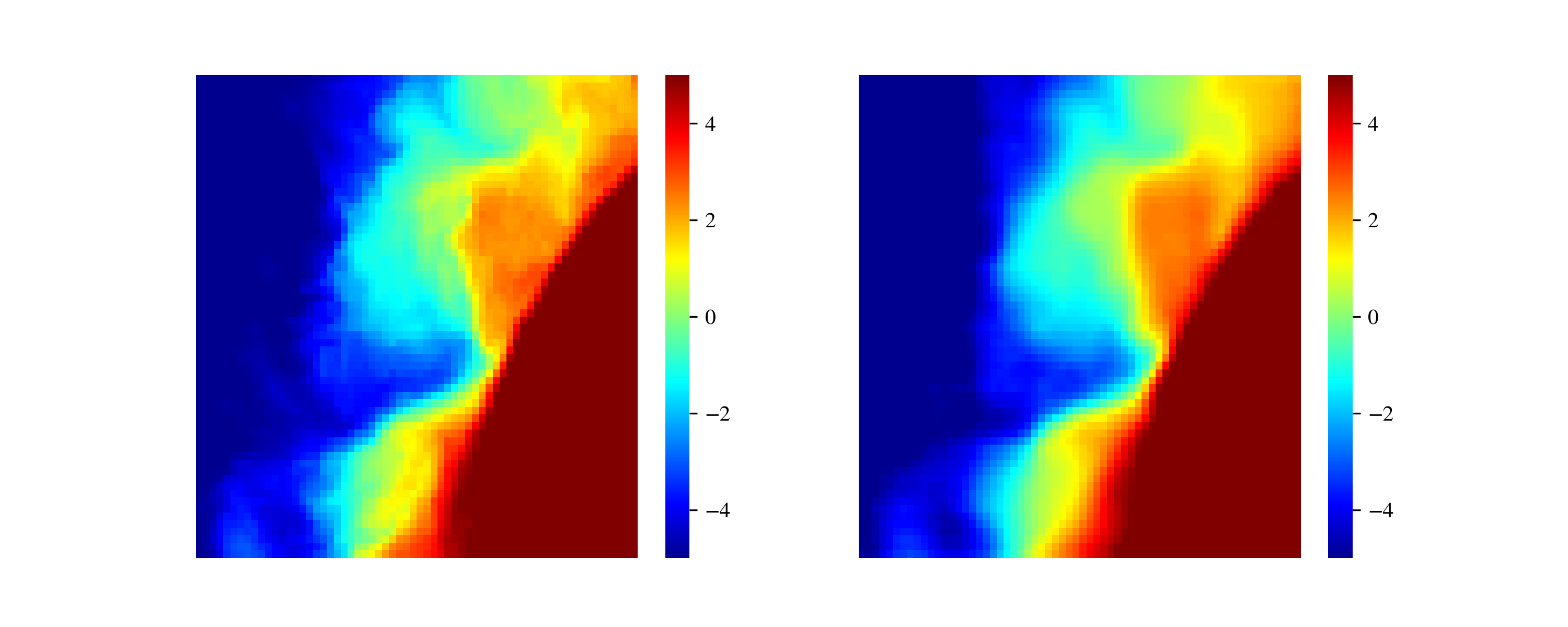
Figure 3: (left) Input cutout, preprocessed as described in $\S$ 3.1. (right) Image generated by the trained autoencoder, which passes the cutout through a 512 unit latent space. As designed, the reproduction captures the gross features but not all of the small-scale detail.

Figure 3 shows an example of a preprocessed input SSTa cutout and the resultant reconstruction cutout from the autoencoder. As designed, the output is a good reconstruction albeit at a lower resolution that does not capture all of the finer features due to the information bottleneck in the autoencoder’s latent space but it does capture the mesoscale structure of the field. For the normalizing flow, we used a cutout batch size of 64 and a learning rate of 0.00025. Similarly, we found $\approx 10$ epochs were sufficient to achieve convergence.

We performed training on the Nautilus distributed computing system with a single GPU. In this training setup, a single epoch for the auto-encoder requires 100 s while a single epoch for the flow requires $\approx 900$ s.

4 Results and Discussion

In this section, we report on the main results of our analysis with primary emphasis on outlier detection. We also begin an exploration of the ulmo model to better understand the implications of deep learning for analyzing remote-sensing imaging; these will be expanded upon in future works.

Figure 4: Distribution of LL values for the full dataset (modulo the training images). The majority are well described by a Gaussian centered at ${\rm LL}\approx 240$, with a tail to much lower LL values. The inset shows the lowest 0.1% sample of LL, which we define as outlier cutouts.

4.1 The outlier cutouts sample

Figure 4 shows the LL distribution for all extracted cutouts modulo the set of training cutouts from 2010. The distribution peaks at LL $\approx 240$ with a tail to very low values. The latter is presented in the inset which shows the lowest 0.1% of the distribution; these define the outlier cutouts of the full sample (or outliers for short).

Figure 5: Incidence (counts) of outlier cutouts broken down by month and year. The primary feature is seasonal, i.e., a higher number of outlier cutouts during boreal winter months than summer. There is also a weak, but possible increase in the incidence of outliers over the past $\sim 10$ years.

The striping apparent in the inset of Figure 4 indicates a non-uniform, temporal dependence in the outlier cutouts. Figure 5 examines this further, plotting the occurrence of outliers as a function of year and month. The only significant trend apparent is seasonal, i.e., a higher incidence of outliers during the boreal winter. We speculate this is due to the predominance of northern hemisphere cutouts/outliers – approximately 60%/64% of the total – and the reduced thermal contrast of northern hemisphere surface waters in the boreal summer. As will be shown, the range of SSTa in a cutout is correlated with the probability of the cutout being identified as an outlier; the larger the range the more likely the cutout will be so flagged. This is especially true in the vicinity of strong currents such as western boundary currents, which separate relatively warm, poleward moving equatorial and subtropical waters from cooler water poleward of the currents. In summer months the cooler water warms substantially faster than the surface water of the current dramatically reducing the contrast between the two water bodies, often masking the dynamical nature of the field in these regions rendering them less atypical. We also see variations during the $\sim 20$ years of the full dataset, including a possible increase over the past $\sim 10$ years. These modest trends aside, ulmo identifies outliers in all months and years of the dataset.

Figure 6: Depiction of the spatial distribution of the outliers discovered by ulmo. These are primarily in the well-known western boundary currents off Japan, North and South America, and South Africa. Note that the scaling is logarithmic.

A question that naturally arises is whether there is any structure to the geographic distribution of outliers. Figure 6 shows the count distribution of the outliers across the entire ocean. Remarkably, the ulmo algorithm has rediscovered that the rarest phenomena occur primarily in western boundary currents – following the continental boundary and/or shortly after separation. These regions of the ocean have been studied extensively because of their highly dynamical nature. In short, the ulmo algorithm identified (or even rediscovered!) without any predisposition a consistent set of dynamically important oceanographic regions.

To a lesser extent, one also finds outliers in the vicinity of the connection between large gulfs or seas and the open ocean – the Gulf of California, the Red Sea and the Mediterranean. Also of interest are the outliers in the Gulf of Tehuantepec. These result from very strong winds blowing from the Gulf of Mexico to the Pacific Ocean through the Chivela Pass, resulting in significant mixing of the near-shore waters.

There are two ways to view the results in Figure 6: (1) as the contrarian, i.e., the ulmo algorithm has simply reproduced decades-old, basic knowledge in physical oceanography on where the most dynamical regions of the ocean lie; or (2) as the optimist, i.e., the ulmo algorithm – without any direction from its developers – has rederived one of the most fundamental aspects of physical oceanography. It has learned central features of the ocean from the patterns of SSTa alone. In this regard, ulmo may hold greater potential/promise to learn and derive other, not-yet-identified behaviors in the ocean.

4.2 Scrutinizing examples of the outliers

Figure 7 shows a gallery of 9 outliers selected to uniformly span time and location in the ocean. These exhibit extreme SSTa variations and/or complexity and (presumably) mark significant mesoscale activity. A common characteristic of these cutouts is the presence of a strong and sharp gradient in SSTa which separates two regions exhibiting a large temperature difference. Typically, such gradients are associated with strong ocean currents, often at mid-latitudes on the western edge of ocean basins. We define a simple statistic of the temperature distribution $\Delta T\equiv T_{90}-T_{10}$ where $T_{X}$ is the temperature at the Xth percentile of a given cutout. All of the outliers in Figure 7 exhibit $\Delta T>7$K, a point we return to in the following sub-section.

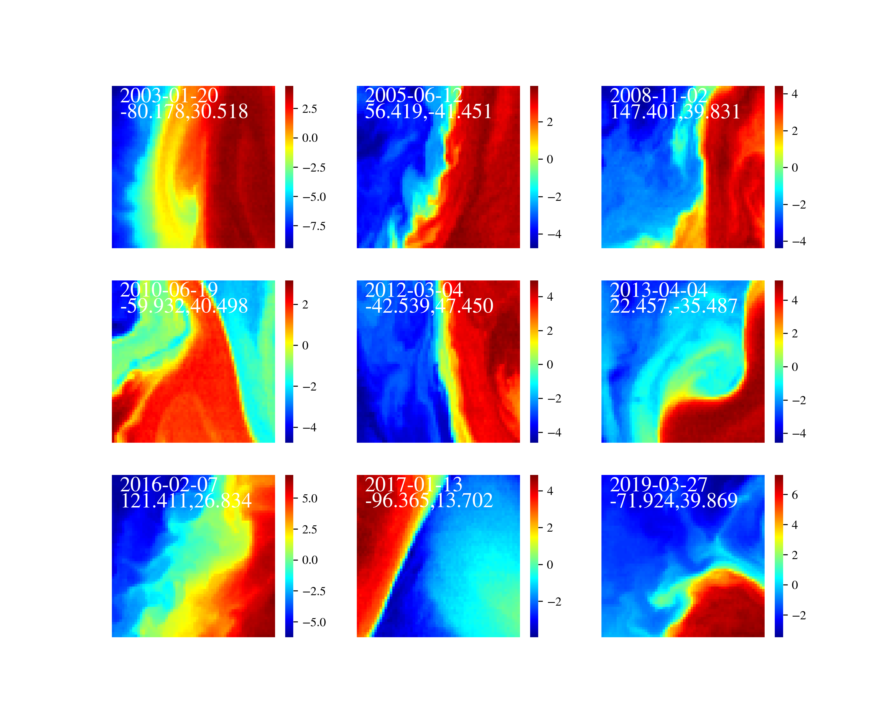
Figure 7: Gallery of outliers drawn from the distribution of cutouts with the lowest 0.1% of LL values. This representative sample was further selected to uniformly sample the $\sim 20$ year interval of the dataset and the spatial distribution (Figure 6). Note the large and complex temperature gradients within all cutouts showing $\Delta T>7$ K. The color bar refers to SSTa in units of Kelvin.

As an example of the anomalous behaviour associated with outlier cutouts, we examine the evolution of the SST field in the vicinity of the 19 June 2010 cutout (Fig. 7) located in the Gulf Stream region; Fig. 8a shows the cutout and (b) its location in the 5-minute granule. We selected this cutout because it is in a region with which we have significant experience. Fig. 9 shows an expanded version of the SST field in the vicinity of the cutout. The main feature in Fig. 9 is the Gulf Stream, the bright red, fading to orange, band meandering from the bottom left hand corner of the image to the middle of the right hand side. A portion of the Gulf Stream loops through the lower half of the cutout and a streamer extends to the north (Fig. 8) from the northernmost excursion of the stream. To aid in the interpretation of this cutout, we make use of the mesoscale eddy dataset produced by Chelton et al. (2011). It shows an eddy, most probably a Warm Core Ring (WCR), moving to the west at approximately 5 km/day to the north of the stream from 17 May (very light gray circle) to 14 June (red circle) when it began to interact with the Gulf Stream, drawing warm Gulf Stream Water on its western side to the north and cold Slope Water on its eastern side to the south. The eddy disappears from the altimeter record two weeks later and is replaced by a very large anticyclone (the dotted black circle) to the west southwest of the eddy’s last position. This is likely a detaching meander of the Gulf Stream resulting from the absorption of the eddy into an already chaotic configuration.

Of particular interest is that the Gulf Stream appears to have lost its coherence between approximately 63^∘ and 59^∘W. Specifically, note the very thin band of cooler water ($\sim 21^{\circ}$C) in the middle of the warm band ($\sim 24^{\circ}$C) of, presumably, Gulf Stream Water between $63.5^{\circ}$ and $62^{\circ}$W and a second similar band (but moving in the opposite direction) between $61.5^{\circ}$ and $60.5^{\circ}$. The western cool band appears to separate one branch of Gulf Stream Water that has been advected from the southwestern edge of the large meander centered at $65.5^{\circ}$W, $38.5^{\circ}$N, and a second branch advected from its southeastern edge. These two branches may result from a general instability of the Gulf Stream associated with formation, or in this case the likely aborted formation, of a WCR. In the normal formation process, the initial state is a large meander of the Gulf Stream and the final state is a relatively straight Gulf Stream with a WCR to the north. In this case the process appears to have begun but inspection of subsequent images suggests that a ring was not formed; the meander reformed after initially beginning the detachment process. However, this is all quite speculative, the important point is that the stream appears to have lost its coherence immediately upstream of the cutout, which we believe to be a very unusual process. Admittedly the cutout only ‘sees’ a very small portion of this but we have found the suggestion of convoluted dynamics in the immediate vicinity of a large fraction of other outliers as well. Bottom line: Cornillon, who has been looking at SST fields derived from satellite-borne sensors for over 40 years, found that more than one-in-ten of the anomalous fields discovered by ULMO suggested intriguing dynamics that he has not previously encountered; recall that this is one-in-ten of one-in-a-thousand (the definition of an outlier) or approximately one field in ten thousand.

Figure 8: The 19 June 2010 cutout of Fig. 7 with LL $=-1234.1$, in the lowest 0.1% of the log-likelihood values for the dataset. a) The original cutout in satellite-coordinates prior to preprocessing. b) The entire granule shown in a plate carrée projection with the continental boundary (dark gray) and the cutout (black rectangle). Note the change of palettes from a to b to accommodate the larger range of SST in b. Light gray are masked pixels, either from clouds, land, or clear pixels improperly flagged as cloud-contaminated ($\S$ 2).

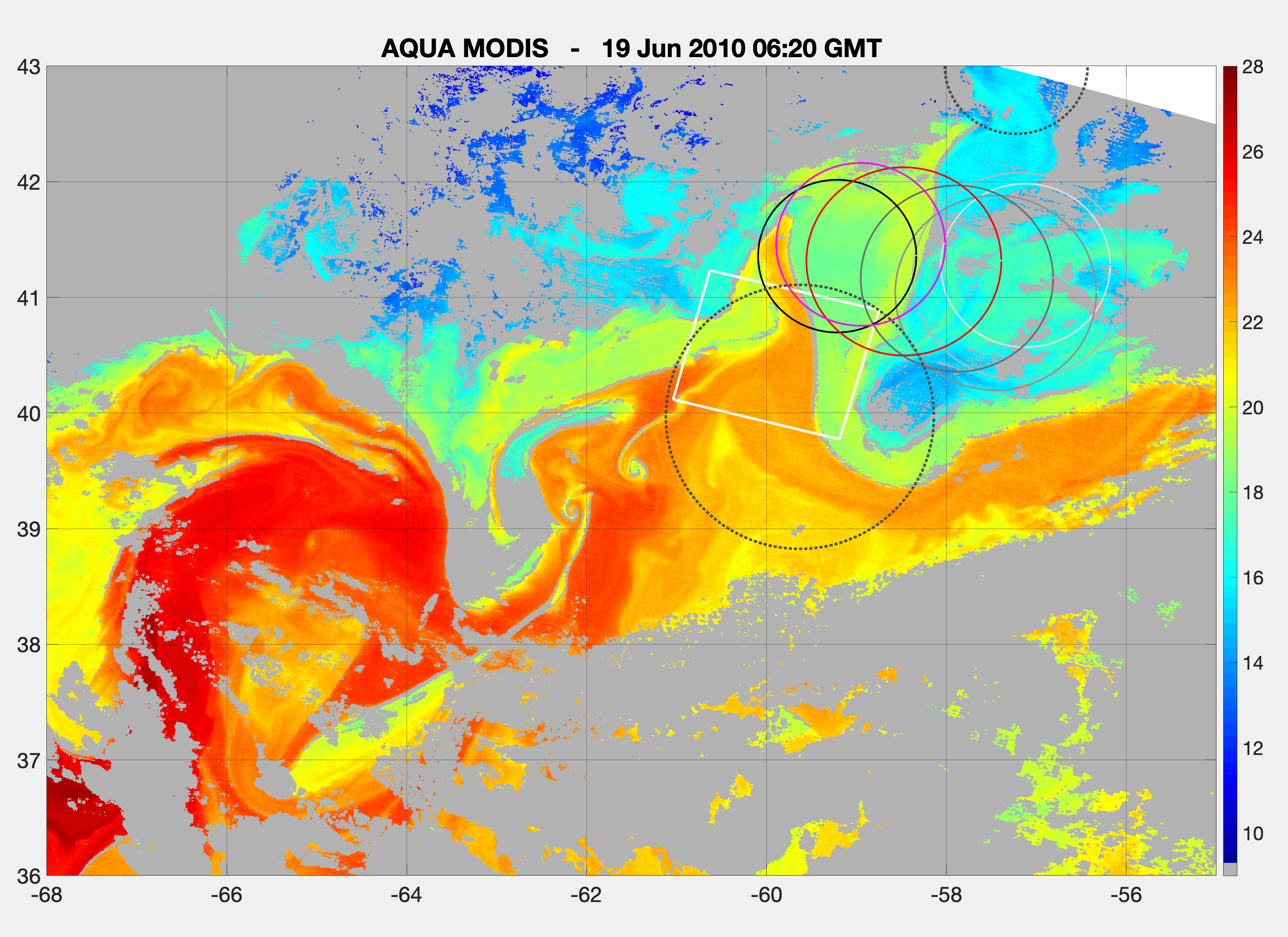
Figure 9: The SST field in the vicinity of the 19 June 2010 cutout of Fig. 7. The cutout (white rectangle) is centered on 60^∘W, 41^∘30”N. Solid circles outline all observations of the anticyclonic eddy identified by Chelton et al. (2011), which passed through the cutout on 19 June 2010. Circles are colored from light gray ($1^{st}$ detection of the eddy on 17 May) to black (last observation on 28 June) with the exception of its location shown in red on 14 June, immediately prior to the satellite overpass, and its location (magenta) one week later, 21 June, immediately following the overpass. Circles with dotted black outlines are anticyclonic eddies found in a broader search ($\pm 3^{\circ}$ centered on 60^∘W, 41^∘30”N) on 5 July, one week after the last observation of the eddy of interest. No cyclonic eddies were found in a similar search. Clouds are light gray.

4.3 Digging Deeper

It is evident from the preceding sub-sections (e.g., Figure 7) that ulmo has discovered a set of highly unusual and dynamic regions of the ocean. Scientifically, this is extremely useful – irrespective of the underlying processes – as it can launch future, deeper inquiry into the physical processes generating such patterns. On the other hand, as scientists we are inherently driven to understand – as best as possible – what/how/why ulmo triggered upon. We begin that process here and defer further exploration to future work.

In Section 4.1, we emphasized that the entire gallery of outliers (Figure 7) exhibits a large temperature variation $\Delta T>7$K. Exploring this further, Figure 10 plots LL vs. $\Delta T$ for the full set of cutouts analyzed. Indeed, the two are anti-correlated with the lowest LL values corresponding to the largest $\Delta T$. This suggests that a simple rules-based algorithm of selecting all cutouts with $\Delta T>10$ K would select the most extreme outliers discovered by ulmo. One may question, therefore, whether a complex and hard-to-penetrate AI model was even necessary to reproduce our results.

Further analysis suggests that there may be more to the distribution of LLs. Specifically, note that there is substantial scatter about the mean relation between LL and $\Delta T$; for example, at LL $=-1000$ one finds $\Delta T$ values ranging from $1-10$ K. Similarly, any cutout with $\Delta T<8$ K includes a non-negligible set of images with ${\rm LL}\gtrsim 0$. Figure 10 indicates that the patterns that ulmo flags as outliers are not solely determined by $\Delta T$.

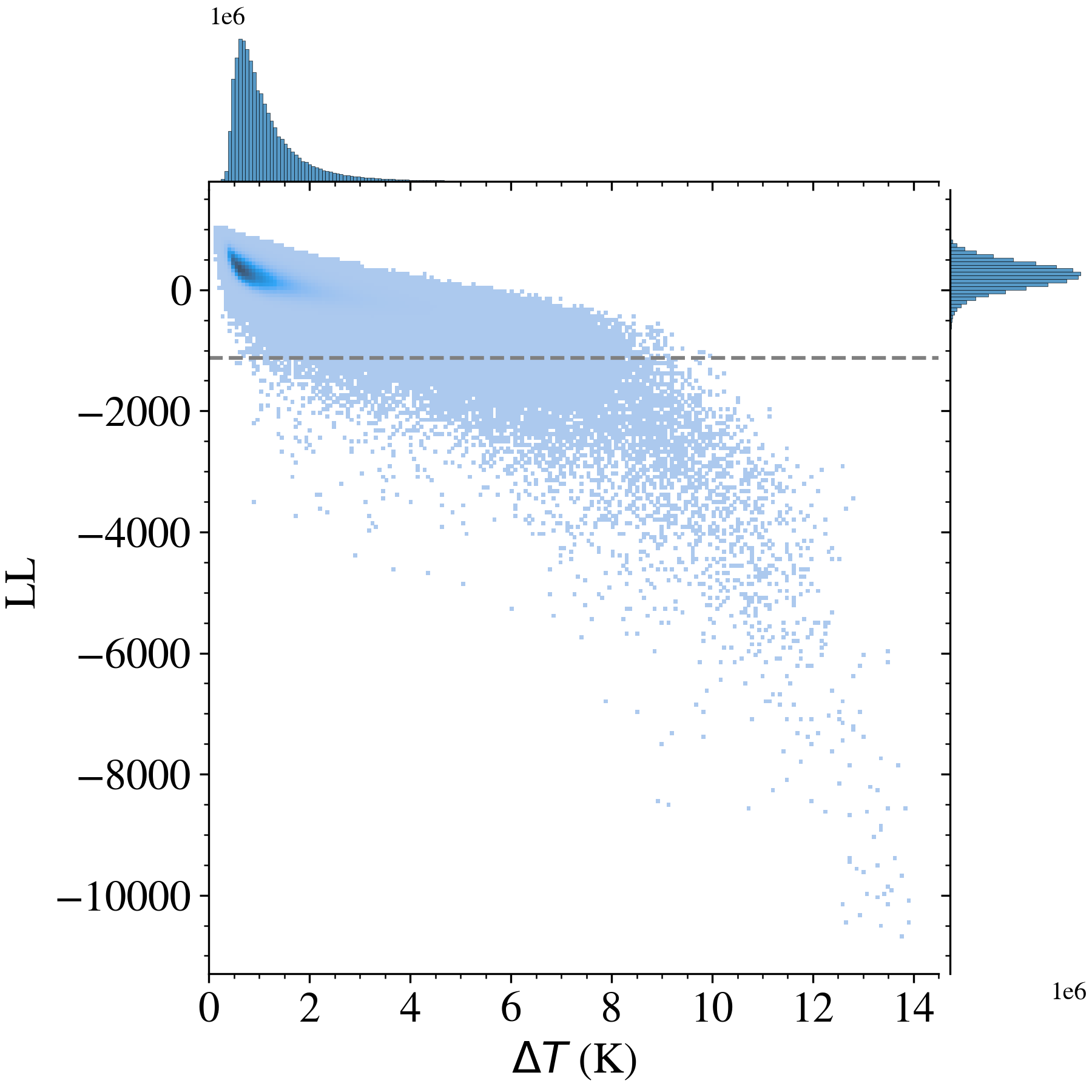
Figure 10: Distribution of LL values as a function of $\Delta T$. While there is a strong anti-correlation apparent, the relationship exhibits substantial scatter such that $\Delta T$ is not a precise predictor of LL nor the underlying SSTa patterns characterized by ulmo. The horizontal line at $\rm LL\approx-1123$ corresponds to the 0.1% threshold; cutouts with log-likelihood values beneath this line are considered to be outliers.

This becomes especially clear in the following exercise. Consider the full set of cutouts within the small range $\Delta T=[2-2.1]$ K. From Figure 10, we see these exhibit ${\rm LL}\approx[-2600,590]$ and find that the LL distribution is well described by a Gaussian (not shown) with $<{\rm LL}>\approx 10$ and $\sigma({\rm LL})\approx 150$. Now consider the cutouts with the lowest/highest 10/90% of the distribution, i.e., the ’outlier’/’inlier’ sub-samples within this small range of $\Delta T$. We refer to these as $LL_{10}$ and $LL_{90}$ cutouts, respectively. Figure 11 shows the spatial distribution of these cutouts. Remarkably, there are multiple areas dominated by only one of the sub-samples (e.g., LL₉₀ cutouts along the Pacific equator). It is evident that ulmo finds large spatial structures in the log-likelihood distribution of cutouts that are independent of $\Delta T$.

Furthermore, there are several locations in the ocean where LL₁₀ and LL₉₀ cutouts are adjacent to one another but still separate. One clear example is within the Brazil-Malvinas Confluence, off the coast of Argentina. Figure 12a shows a zoom-in of that region with the colors corresponding to the LL values (not strictly the LL₁₀ or LL₉₀ distributions shown in Fig. 11). Figure 12a highlights the clear and striking separation of the LL values in this region as do the histograms (Figure 12b) for the LL values of cutouts in the two rectangles shown in panel a. The dynamics of the ocean in this region is well-studied Piola et al. (2018). Higher LL regions tend to be found on the Patagonian Shelf where the dynamics are dominated by tides, buoyancy and wind–forcing the circulation at the local level–and off-shore currents–forcing the circulation remotely. In contrast, the lower LL regions track more dynamic, current-driven motions of the main Brazil-Malvinas Confluence. Of particular interest is the rather abrupt switch at $\sim 40^{\circ}$S from higher LL values to the south to lower values to the north. This is consistent with the observation of Combes & Matano (2018), based on numerical simulations, that “[t]here is an abrupt change of the dynamical characteristics of the shelf circulation at 40^∘S”. They attribute this change in dynamics to this region being a sink for Patagonian Shelf waters, which are being advected offshore by the confluence of the Brazil and Malvinas Currents. Again, ulmo has captured striking detail in regional dynamics with no directed input. Further analysis of the region (not shown) suggests that ulmo has also captured seasonal differences in the dynamics, with a region of lower LL cutouts in waters approximately 100 m deep between $38^{\circ}$ and $45^{\circ}$S in austral winter but not austral summer.

Figure 11: Spatial distribution of the LL₁₀/LL₉₀ cutouts (red/blue) defined as the upper/lower tenth percentile of the LL distribution for the set of cutouts with $\Delta T=[2,2.1]$ K. It is evident that these cutouts occupy distinct regions of the ocean, i.e., the ulmo algorithm has identified patterns with significant spatial coherence. More remarkable, note the several areas (e.g. in the Brazil-Malvinas current) where one identifies adjacent but separate patches of LL₉₀ and LL₁₀ cutouts.

Intrigued by ulmo’s ability to spatially separate these regions based on SSTa patterns alone, we inspected a set of 25 randomly selected samples from R1, the eastern rectangle in Figure 12a, and 25 randomly selected samples from R2 to further explore its inner-workings (see lower panels of Figure 12). The comparison is striking and we easily identify qualitative differences in the observed patterns despite their nearly identical $\Delta T$ values. The higher LL cutouts show large-scale gradients and features with significant coherence whereas the lower LL cutouts exhibit gradients and features with a broader range of scales and a suggested richer distribution of relative vorticity.

Another area, which stands out in Figure 11, is that in the Northwest Atlantic where a region of LL₉₀ cutouts (red) are surrounded by LL₁₀ cutouts (blue). The structure (not shown) of the LL₉₀ cutouts in this region, which are on the Grand Banks of Newfoundland, resemble the structure of the LL₉₀ cutouts shown in Figure 12 and the structure of the LL₁₀ cutouts in this region is much closer to that of the LL₁₀ cutouts shown in Figure 12 than to the LL₉₀ cutouts in either region. In fact, a gallery of randomly selected LL₉₀ cutouts from the world ocean are similar to those off of Argentina and Newfoundland and a gallery of randomly selected LL₁₀ cutouts from the world ocean are more similar to the LL₁₀ cutouts off of Argentina and Newfoundland than to the LL₉₀ cutouts. Simply put, the structure of the SST cutouts shown in blue in Figure 11 tend to be similar to one another and quite different from those shown in red although the cutouts in both cases have virtually the same dynamic ranges in SST. This observation raises intriguing questions about the similarities and the differences in upper ocean processes in these regions – questions to be addressed in further analyses of the fields.

Figure 12: (a) Distribution of the LL values for cutouts near the Brazil-Malvinas Confluence, restricted to those with temperature difference $\Delta T\approx 2$ K. One identifies a clear separation, where the lower LL values lie within the current and the higher values lie close to the Argentinian coast. Marked are two rectangles (R1, R2), one in each region, referred to in the other panels. Also marked is the 200m bathymetry described in the text. (b) Histograms of the LL values for the cutouts from two regions (R1/R2) chosen to show lower/higher LL values near the confluence. (lower panels) Representative cutouts from each subset – the left set are drawn from the R2 rectangle and therefore exhibit higher LL values. The right set are from R1. These galleries reveal qualitative differences in the SST patterns, i.e., unique ocean dynamics. The palette for the lower panels ranges linearly from $-1$ to 1 K.

We can capture some of the differences between the higher/lower LL sub-samples of Figure 12 with another simple statistic – the RMS in SSTa, $\sigma_{T}$. On average, the lower LL cutouts exhibit $\approx 9\%$ higher $\sigma_{T}$ than those with a higher LL. Furthermore, we find LL correlates with $\sigma_{T}$ in a fashion similar to $\Delta T$. On the other hand, it is evident from Figure 12 that there is significant structure apparent in the cutouts that is not described solely by $\sigma_{T}$. The correlations of LL with $\Delta T$ and $\sigma_{T}$ manifest from the underpinnings of ulmo: the distribution of ocean SSTa patterns reflect the distribution of simple statistics like $\Delta T$ or $\sigma_{T}$, which exhibit large and non-uniform variations across the ocean. The complexity of these patterns, however, belie the information provided by simple statistics alone.

5 Conclusions and Future Work

With the design and application of a machine learning algorithm ulmo, we set out to identify the rarest sea surface temperature patterns in the ocean through an out-of-distribution analysis yielding a unique log-likelihood (LL) value for every cutout. On this goal, we believe we were successful (e.g., Figures 6,7). In examining the nature of the outliers we found that these exhibited extrema of two simple metrics: the temperature difference $\Delta T$ and standard deviation $\sigma_{T}$. With the full privilege of hindsight, we expect that any metric introduced to describe the cutouts which exhibits a broad and non-uniform distribution would correlate with LL. However, no single metric can capture the inherent pattern complexity and therefore none correlates tightly with LL (Figure 10).

Looking to the future, the greatest potential of algorithms like ulmo may be that the patterns it learns are more fundamental than measures traditionally implemented in the scientific community (e.g., Fast Fourier Transform (FFT), Empirical Orthogonal Function EOF). We hypothesize that the mathematical nature of convolutional neural networks CNN – convolutional features and max-pooling, which synthesizes data across the scene while remaining invariant to translation – captures aspects of the data that EOF analysis could not (nor any other simple linear approach). Indeed, referring back to Figure 12, while as humans we trivially distinguish between the two sets of cutouts marking the ocean dynamics in the Brazil-Malvinas Confluence and can identify metrics on which they differ, these metrics offer incomplete descriptions. Going forward, we will determine the extent (e.g., via analysis of ocean model outputs) to which the patterns mark fundamental, dynamical processes within the ocean. Potentially, the patterns learned by ulmo (or its successors) hold the optimal description of any such phenomena.

As emphasized at the onset, this manuscript offers only a first glimpse at the potential for applying advanced artificial intelligence techniques to the tremendous ocean datasets obtained from satellite-borne sensors. The techniques introduced here will translate seamlessly to sea surface height or ocean color imaging to identify extrema/complexity in geostrophic currents and biogeochemical processes. These too will be the focus of future works.

ACRONYMS

(A)ATSR

one or all of ATSR, ATSR-2 and AATSR

AATSR

Advanced Along Track Scanning Radiometer

ACC

Antarctic Circumpolar Current

ACCESS

Advancing Collaborative Connections for Earth System Science

ACL

Access Control List

ACSPO

Advanced Clear Sky Processor for Oceans

ADA

Automatic Detection Algorithm

ADCP

Acoustic Doppler Current Profiler

ADT

absolute dynamic topography

AESOP

Assessing the Effects of Submesoscale Ocean Parameterizations

AGU

American Geophysical Union

AI

Artificial Intelligence

AIRS

Atmospheric Infrared Sounder

AIS

Ancillary Information Service

AIST

Advanced Information Systems Techonology

AISR

Applied Information Systems Research

ADL

Alexandria Digital Library

API

Application Program Interface

APL

Applied Physics Laboratory

API

Application Program Interface

AMSR

Advanced Microwave Scanning Radiometer

AMSR2

Advanced Microwave Scanning Radiometer 2

AMSR-E

Advanced Microwave Scanning Radiometer - EOS

ANN

Artificial Neural Network

AOOS

Alaska Ocean Observing System

APAC

Australian Partnership for Advanced Computing

APDRC

Asia-Pacific Data-Research Center

ARC

ATSR Reprocessing for Climate

ASCII

American Standard Code for Information Interchange

AS

Aggregation Server

ASFA

Aquatic Sciences and Fisheries Abstracts

ASTER

Advanced Spaceborne Thermal Emission and Reflection Radiometer

ATBD

Algorithm Theoretical Basis Document

ATSR

Along Track Scanning Radiometer

ATSR-2

Second ATSR

AVISO

Archiving, Validation and Interpretation of Satellite Oceanographic Data

ANU

Australian National University

AVHRR

Advanced Very High Resolution Radiometer

AzC

Azores Current

BAA

Broad Agency Announcement

BAO

bi-annual oscillation

BES

Back-End Server

BMRC

Bureau of Meteorology Research Centre

BOM

Bureau of Meteorology

BT

brightness temperature

BUFR

Binary Universal Format Representation

CAN

Cooperative Agreement Notice

CAS

Community Authorization Service

CC

cloud cover

CCA

Cayula-Cornillon Algoritm

CCI

Climate Change Initiative

CCLRC

Council for the Central Laboratory of the Research Councils

CCMA

Center for Coastal Monitoring and Assessment

CCR

cold core ring

CCS

California Current System

CCSM

Community Climate System Model

CCSR

Center for Climate System Research

CCV

Center for Computation and Visualization

CDAT

Climate Data Analysis Tools

CDC

Climate Diagnostics Center

CDF

Common Data Format

CDR

Common Data Representation

CEDAR

Coupled Energetic and Dynamics and Atmospheric Regions

CEOS

Committee on Earth Observation Satellites

CERT

Computer Emergency Response Team

CenCOOS

Central & Northern California Ocean Observing System

CF

clear fraction

CGI

Common Gateway Interface

CHAP

CISL High Performance Computing Advisory Panel

CIFS

Common Internet File System

CIMSS

Cooperative Institute for Meteorological Satellite Studies

CIRES

Cooperative Institute for Research (in) Environmental Sciences

CISL

Computational & Information Systems Laboratory

CLASS

Comprehensive Large Array-data Stewardship System

CLIVAR

Climate Variability and Predictability

CLS

Collecte Localisation Satellites

CME

Community Modeling Effort

CMS

Centre de Météorologie Spatiale

CNN

Convolutional Neural Network

COA

Climate Observations and Analysis

COARDS

Cooperative Ocean-Atmosphere Research Data Standard

COAPS

Center for Ocean-Atmospheric Prediction Studies

COBIT

Control Objectives for Information and related Technology

COCO

CCSR Ocean Component model

CODAR

Coastal Ocean Dynamics Applications Radar

CODMAC

Committee on Data Management, Archiving, and Computing

Co-I

Co-Investigator

CORBA

Common Object Request Broker Architecture

COLA

Center for Ocean-Land-Atmosphere Studies

CPU

Central Processor Unit

CRS

Coordinate Reference System

CSA

Cambridge Scientific Abstracts

CSC

Coastal Services Center

CSIS

Center for Strategic and International Studies

CSL

Constraint Specification Language

CSP

Chermayeff, Sollogub and Poole, Inc.

CSDGM

Content Standard for Digital Geospatial Metadata

CSV

Comma Separated Values

CTD

Conductivity, Temperature and Salinity

CVSS

Common Vulnerability Scoring System

CZCS

Coastal Zone Color Scanner

DAAC

Distribute Active Archive Center

DAARWG

Data Archiving and Access Requirements Working Group

DAP

Data Access Protocol

DAS

Data set Attribute Structure

DBMS

Data Base Management System

DBDB2

Digital Bathymetric Data Base

DChart

Dapper Data Viewer

DDS

Data Descriptor Structure

DDX

XML version of the combined DAS and DDS

DFT

Discrete Fourier Transform

DIF

Directory Interchange Format

DISC

Data and Information Services Center

DIMES

Diapycnal and Isopycnal Mixing Experiment: Southern Ocean

DMAC

Data Management and Communications committee

DMR

Department of Marine Resources

DMSP

Defense Meteorological Satellite Program

DoD

Department of Defense

DODS

Distributed Oceanographic Data System

DOE

Department of Energy

DSP

U. Miami satellite data processing software

DSS

direct statistical simulation

EASy

Environmental Analysis System

ECCO

Estimating the Circulation and Climate of the Ocean

ECCO2

Estimating the Circulation and Climate of the Ocean Phase II

ECS

EOSDIS Core System

ECHO

Earth Observing System Clearinghouse

ECMWF

European Centre for Medium-range Weather Forecasting

ECV

Essential Climate Variable

EDC

Environmental Data Connector

EDJ

Equatorial Deep Jet

EDFT

Extended Discrete Fourier Transform

EDMI

Earth Data Multi-media Instrument

EEJ

Extra-Equatorial Jet

EIC

Equatorial Intermediate Current

EICS

Equatorial Intermediate Current System

EJ

Equatorial Jets

EKE

eddy kinetic energy

EMD

Empirical Mode Decomposition

EOF

Empirical Orthogonal Function

EOS

Earth Observing System

EOSDIS

Earth Observing System Data Information System

EPA

Environmental Protection Agency

EPSCoR

Experimental Program to Stimulate Competitive Research

EPR

East Pacific Rise

ERD

Environmental Research Division

ERS

European Remote-sensing Satellite

ESA

European Space Agency

ESDS

Earth Science Data Systems

ESDSWG

Earth Science Data Systems Workign Group

ESE

Earth Science Enterprise

ESG

Earth System Grid

ESG II

Earth System Grid – II

ESIP

Earth Science Information Partner

ESMF

Earth System Modeling Framework

ESML

Earth System Markup Language

ESP

eastern South Pacfic

ESRI

Environmental Systems Research Institute

ESR

Earth and Space Research

ETOPO

Earth Topography

EUC

Equatorial Undercurrent

EUMETSAT

European Organisation for the Exploitation of Meteorological Satellites

Ferret

FASINEX

Frontal Air-Sea Interaction Experiment

FDS

Ferret Data Server

FFT

Fast Fourier Transform

FGDC

Federal Geographic Data Committee

FITS

Flexible Image (or Interchange) Transport System

FLOPS

FLoating point Operations Per Second

FRTG

Flow Rate Task Group

FreeForm

FNMOC

Fleet Numerical Meteorology and Oceanography Center

FSU

Florida State University

FTE

Full Time Equivalent

ftp

File Transport Protocol

ftp

File Transport Protocol

GAC

Global Area Coverage

GAN

Generative Adversarial Network

GB

GigaByte - $10^{9}$ bytes

GCMD

Global Change Master Directory

GCM

general circulation model

GCOM-W1

Global Change Observing Mission - Water

GCOS

Global Climate Observing System

GDAC

Global Data Assembly Center

GDS

GrADS Data Server

GDS2

GHRSST Data Processing Specification v2.0

GEBCO

General Bathymetric Charts of the Oceans

GeoTIFF

Georeferenced Tag Image File Format

GEO-IDE

Global Earth Observation Integrated Data Environment

GES DIS

Goddard Earth Sciences Data and Information Services Center

GEMPACK

General Equilibrium Modelling PACKage

GEOSS

Global Earth Observing System of Systems

GFDL

Geophysical Fluid Dynamics Laboratory

GFD

Geophysical Fluid Dynamics

GHRSST

Group for High Resolution Sea Surface Temperature

GHRSST-PP

GODAE High Resolution Sea Surface Temperature Pilot Project

GINI

GOES Ingest and NOAA/PORT Interface

GIS

Geographic Information Systems

Globus

GMAO

Global Modeling and Assimilation Office

GML

Geography Markup Language

GMT

Generic Mapping Tool

GODAE

Global Ocean Data Assimilation Experiment

GOES

Geostationary Operational Environmental Satellites

GOFS

Global Ocean Forecasting System

GoMOOS

Gulf of Maine Ocean Observing System

GOOS

Global Ocean Observing System

GOSUD

Global Ocean Surface Underway Data

GPFS

General Parallel File System

GPU

Graphics Processing Unit

GRACE

Gravity Recovery and Climate Experiment

GRIB

GRid In Binary

GrADS

Grid Analysis and Display System

GridFTP

FTP with GRID enhancements

GRIB

GRid in Binary

GPS

Global Positioning System

GSFC

Goddard Space Flight Center

GSI

Grid Security Infrastructure

GSO

Graduate School of Oceanography

GTSPP

Global Temperature and Salinity Profile Program

GUI

Graphical User Interface

GS

Gulf Stream

HAO

High Altitude Observatory

HLCC

Hawaiian Lee Countercurrent

HCMM

Heat Capacity Mapping Mission

HDF

Hierarchical Data Format

HDF-EOS

Hierarchical Data Format - EOS

HEC

High-End Computing

HF

High Frequency

HGE

High Gradient Event

HPC

High Performance Computing

HPCMP

High Performance Computing Modernization Program

HPSS

High Performance Storage System

HR DDS

High Resolution Diagnostic Data Set

HRPT

High Resolution Picture Transmission

HTML

Hyper Text Markup Language

html

Hyper Text Markup Language

http

the hypertext transport protocol

HTTP

Hyper Text Transfer Protocol

HTTPS

Secure Hyper Text Transfer Protocol

HYCOM

HYbrid Coordinate Ocean Model

I-band

imagery resolution band

IDD

Internet Data Distribution

IB

Image Band

IBL

internal boundary layer

IBM

Internation Business Machines

ICCs

Intermediate Countercurrents

IDE

Integrated Development Environment

IDL

Interactive Display Language

IDLastro

IDL Astronomy User’s Library

IDV

Integrated Data Viewer

IEA

Integrated Ecosystem Assessment

IEEE

Institute (of) Electrical (and) Electronic Engineers

IETF

Internet Engineering Task Force

IFREMER

Institut Français de Recherche pour l’Exploitation de la MER

IMAPRE

El Instituto del Mar del Perú

IMF

Intrinsic Mode Function

IOOS

Integrated Ocean Observing System

ISAR

Infrared Sea surface temperature Autonomous Radiometer

ISO

International Organization for Standardization

ISSTST

Interim Sea Surface Temperature Science Team

IT

Information Technology

ITCZ

Intertropical Convergence Zone

IP

Internet Provider

IPCC

Intergovernmental Panel on Climate Change

IPRC

International Pacific Research Center

IR

Infrared

IRI

International Research Institute for Climate and Society

ISO

International Standards Organization

JASON

JASON Foundation for Education

JDBC

Java Database Connectivity

JFR

Juan Fernández Ridge

JGOFS

Joint Global Ocean Flux Experiment

JHU

Johns Hopkins University

JPL

Jet Propulsion Laboratory

JPSS

Joint Polar Satellite System

KDE

Kernel Density Estimation

KVL

Keyword-Value List

KML

Keyhole Markup Language

KPP

K-Profile Parameterization

LAC

Local Area Coverage

LAN

Local Area Network

LAS

Live Access Server

LASCO

Large Angle and Spectrometric Coronagraph Experiment

LatMIX

Scalable Lateral Mixing and Coherent Turbulence

LDAP

Lightweight Directory Access Protocol

LDEO

Lamont Doherty Earth Observatory

LEAD

Linked Environments for Atmospheric Discovery

LEIC

Lower Equatorial Intermediate Current

LES

Large Eddy Simulation

L1

Level-1

L2

Level-2

L3

Level-3

L4

Level-4

LL

log-likelihood

LLC

Latitude/Longitude/polar-Cap

LLC-4320

Latitude/Longitude/polar-Cap (LLC)-4320

LLC-2160

LLC-2160

LLC-1080

LLC-1080

LHF

Latent Heat Flux

LST

local sun time

LTER

Long Term Ecological Research Network

LTSRF

Long Term Stewardship and Reanalysis Facility

LUT

Look Up Table

M-band

moderate resolution band

MABL

marine atmospheric boundary layer

MADT

Maps of Absolute Dynamic Topography

MapServer

MapServer

MAT

Metadata Acquisition Toolkit

MATLAB

MARCOOS

Mid-Atlantic Coastal Ocean Observing System

MARCOORA

Mid-Atlantic Coastal Ocean Observing Regional Association

MB

MegaByte - $10^{6}$ bytes

MCC

Maximum Cross-Correlation

MCR

MATLAB Component Runtime

MCSST

Multi-Channel Sea Surface Temperature

MDT

mean dynamic topography

MDB

Match-up Data Base

MDOT

mean dynamic ocean topography

MEaSUREs

Making Earth System data records for Use in Research Environments

MERRA

Modern Era Retrospective-Analysis for Research and Applications

MERSEA

Marine Environment and Security for the European Area

MTF

Modulation Transfer Function

MICOM

Miami Isopycnal Coordinate Ocean Model

MIRAS

Microwave Imaging Radiometer with Aperture Synthesis

MITgcm

MIT General Circulation Model

MIT

Massachusetts Institute of Technology

mks

meters, kilograms, seconds

MLP

Multilayer Perceptron

MLSO

Mauna Loa Solar Observatory

MM5

Mesoscale Model

MMI

Marine Metadata Initiative

MMS

Minerals Management Service

MODAS

Modular Ocean Data Assimilation System

MODIS

MODerate-resolution Imaging Spectroradiometer

MOU

Memorandum of Understanding

MPARWG

Metrics Planning and Reporting Working Group

MSE

mean square error

MSG

Meteosat Second Generation

MTPE

Mission To Planet Earth

MUR

Multi-sensor Ultra-high Resolution

MV

Motor Vessel

NAML

National Association of Marine Laboratories

NAHDO

National Association of Health Data Organizations

NAS

Network Attached Storage

NASA

National Aeronautics and Space Administration

NCAR

National Center for Atmospheric Research

NCEI

National Centers for Environmental Information

NCEP

National Centers for Environmental Prediction

NCDC

National Climatic Data Center

NCDDC

National Coastal Data Development Center

NCL

NCAR Command Language

ncBrowse

NcML

netCDF Markup Language

NCO

netCDF Operator

NCODA

Navy Coupled Ocean Data Assimilation

NCSA

National Center for Supercomputing Applications

NDBC

National Data Buoy Center

NDVI

Normalized Difference Vegetation Index

NEC

North Equatorial Current

NECC

North Equatorial Countercurrent

NEFSC

Northeast Fisheries Science Center

NEIC

North Equatorial Intermediate Current

netCDF

NETwork Common Data Format

NEUC

North Equatorial Undercurrent

NGDC

National Geophysical Data Center

NICC

North Intermediate Countercurrent

NIST

National Institute of Standards and Technology

NLSST

Non-Linear Sea Surface Temperature

NMFS

National Marine Fisheries Service

NMS

New Media Studio

NN

Neural Network

NOAA

National Oceanic and Atmospheric Administration

NODC

National Oceanographic Data Center

NOGAPS

Navy Operational Global Atmospheric Prediction System

NOMADS

NOAA Operational Model Archive Distribution System

NOPP

National Oceanographic Parternership Program

NOS

National Ocean Service

NPP

National Polar-orbiting Partnership

NPOESS

National Polar-orbiting Operational Environmental Satellite System

NSCAT

NASA SCATterometer

NSEN

NASA Science and Engineering Network

NSF

National Science Foundation

NSIPP

NASA Seasonal-to-Interannual Prediction Project

NRA

NASA Research Announcement

NRC

National Research Council

NRL

Naval Research Laboratory

NSCC

North Subsurface Countercurrent

NSF

National Science Foundation

NSIDC

National Snow and Ice Data Center

NSPIRES

NASA Solicitation and Proposal Integrated Review and Evaluation System

NSSDC

National Space Science Data Center

NVODS

National Virtual Ocean Data System

NWP

Numerical Weather Prediction

NWS

National Weather Service

OBPG

Ocean Biology Processing Group

OB.DAAC

Ocean Biology DAAC

ODC

OPeNDAP Data Connector

OC

ocean color

OCAPI

OPeNDAP C API

ODSIP

Open Data Services Invocation Protocol

OFES

Ocean Model for the Earth Simulator

OCCA

OCean Comprehensive Atlas

OGC

Open Geospatial Consortium

OGCM

ocean general circulation model

OISSTv1

Optimally Interpolated SST Version 1

ONR

Office of Naval Research

OLCI

Ocean Land Colour Instrument

OLFS

OPeNDAP Lightweight Front-end Server

OOD

out-of-distribution

OOPC

Ocean Observation Panel for Climate

OPeNDAP

Open source Project for a Network Data Access Protocol

OPeNDAPg

GRID-enabled OPeNDAP tools

OpenGIS

OpenGIS

OSI SAF

Ocean and Sea Ice Satellite Application Facility

OSS

Office of Space Science

OSTM

Ocean Surface Topography Mission

OSU

Oregon State University

OS X

OWL

Web Ontology Language

OWASP

Open Web Application Security Project

PAE

probabilistic autoencoder

PBL

planetary boundary layer

PCA

Principal Components Analysis

PDF

probability distribution function

PDF

probability density function

PF

Polar Front

PFEL

Pacific Fisheries Environmental Laboratory

PI

Principal Investigator

PIV

Particle Image Velocimetry

PL

Project Leader

PM

Project Member

PMEL

Pacific Marine Environmental Laboratory

POC

particulate organic carbon

PO-DAAC

Physical Oceanography – Distributed Active Archive Center

POP

Parallel Ocean Program

PSD

Power Spectral Density

PSPT

Precision Solar Photometric Telescope

PSU

Pennsylvania State University

PyDAP

Python Data Access Protocol

PV

potential vorticity

QC

quality control

QG

quasi-geostrophic

QuikSCAT

Quick Scatterometer

QZJ

quasi-zonal jet

R2HA2

Rescue & Reprocessing of Historical AVHRR Archives

RAFOS

SOFAR, SOund Fixing And Ranging, spelled backward

RAID

Redundant Array of Independent Disks

RAL

Rutherford Appleton Laboratory

RDF

Resource Description Language

REASoN

Research, Education and Applications Solutions Network

REAP

Realtime Environment for Analytical Processing

ReLU

Rectified Linear Unit

REU

Research Experiences for Undergraduates

RFA

Research Focus Area

RFI

Radio Frequency Interference

RFC

Request For Comments

R/GTS

Regional/Global Task Sharing

RSI

Research Systems Inc.

RISE

Radiative Inputs from Sun to Earth

rms

root mean square

RMI

Remote Method Invocation

ROMS

Regional Ocean Modeling System

ROSES

Research Opportunities in Space and Earth Sciences

RSMAS

Rosenstiel School of Marine and Atmospheric Science

RSS

Remote Sensing Sytems

RTM

radiative transfer model

SACCF

Southern ACC Front

(SAC)-D

Satélite de Aplicaciones Científicas-D

SAF

Subantarctic Front

SAIC

Science Applications International Corporation

SANS

SysAdmin, Audit, Networking, and Security

SAR

synthetic aperature radar

SATMOS

Service d’Archivage et de Traitement Météorologique des Observations Spatiales

SBE

Sea-Bird Electronics

SciDAC

Scientific Discovery through Advanced Computing

SCC

Subsurface Countercurrent

SCCWRP

Southern California Coastal Water Research Project

SDAC

Solar Physics Data Analysis Center

SDS

Scientific Data Set

SDSC

San Diego Supercomputer Center

SeaDAS

SeaWiFS Data Analysis System

SeaWiFS

Sea-viewing Wide Field-of-view Sensor

SEC

South Equatorial Current

SECC

South Equatorial Countercurrent

SECDDS

Sun Earth Connection Distributed Data Services

SEEDS

Strategic Evolution of ESE Data Systems

SEIC

South Equatorial Intermediate Current

SEUC

Southern Equatorial Undercurrent

SEVIRI

Spinning Enhanced Visible and Infra-Red Imager

SeRQL

SeRQL

SGI

Silican Graphics Incorporated

SHF

Sensible Heat Flux

SICC

South Intermediate Countercurrent

SIED

single image edge detection

SIPS

Science Investigator–led Processing System

SIR

Scatterometer Image Reconstruction

SISTeR

Scanning Infrared Sea Surface Temperature Radiometer

SLA

sea level anomaly

SMAP

Soil Moisture Active Passive

SMMR

Scanning Multichannel Microwave Radiometer

SMOS

Soil Moisture and Ocean Salinity

SMTP

Simple Mail Transfer Protocol

SOAP

Simple Object Access Protocol

SOEST

School of Ocean and Earth Science and Technology

SOFAR

SOund Fixing And Ranging

SOFINE

Southern Ocean Finescale Mixing Experiment

SOHO

Solar and Heliospheric Observatory

SPARC

Space Physics and Aeronomy Research Collaboratory

SPARQL

Simple Protocol and RDF Query Language

SPASE

Space Physics Archive Search Engine

SPCZ

South Pacific Convergence Zone

SPDF

Space Physics Data Facility

SPDML

Space Physics Data Markup Language

SPG

Standards Process Group

SQL

Structured Query Language

SSCC

South Subsurface Countercurrent

SSL

Secure Sockets Layer

SSO

Single sign-on

SSES

Single Sensor Error Statistics

SSH

sea surface height

SSHA

sea surface height anomaly

SSMI

Special Sensor Microwave/Imager

SST

sea surface temperature

SSTa

SSTa

SSS

sea surface salinity

SSTST

Sea Surface Temperature Science Team

STEM

science, technology, engineering and mathematics

STL

Standard Template Library

STCZ

Subtropical Convergence Zone

Suomi-NPP

Suomi-National Polar-orbiting Partnership

SWEET

Semantic Web for Earth and Environmental Terminology

SWFSC

Southwest Fisheries Science Center

SWOT

Surface Water and Ocean Topography

SWRL

Semantic Web Rule Language

SubEx

Submesoscale Experiment

SURA

Southeastern Universities Research Association

SURFO

Summer Undergraduate Research Fellowship Program in Oceanography

SuperDARN

Super Dual Auroral Radar Network

TAMU

Texas A&M University

TB

TeraByte - $10^{12}$ bytes

TCASCV

Technology Center for Advanced Scientific Computing and Visualization

TCP

Transmission Control Protocol

TCP/IP

Transmission Control Protocol/Internet Protocol

TDS

THREDDS Data Server

TEX

external temperature or T-External

THREDDS

Thematic Realtime Environmental Data Distributed Services

TIDI

TIMED Doppler Interferometer

TIFF

Tag Image File Format

TIMED

Thermosphere, Ionosphere, Mesosphere, Energetics and Dynamics

TLS

Transport Layer Security

TRL

Technology Readiness Level

TMI

TRMM Microwave Imager

TOPEX/Poseidon

TOPography EXperiment for Ocean Circulation/Poseidon

TRMM

Tropical Rainfall Measuring Mission

TSG

thermosalinograph

UCAR

University Corporation for Atmospheric Research

UCSB

University of California, Santa Barbara

UCSD

University of California, San Diego

uCTD

Underway Conductivity, Temperature and Salinity or Underway CTD

UDDI

Universal Description, Discovery and Integration

UMAP

Uniform Manifold Approximation and Projection

UMiami

University of Miami

Unidata

URI

University of Rhode Island

UPC

Unidata Program Committee

URL

Uniform Resource Locator

USGS

United States Geological Survey

UTC

Coordinated Universal Time

UW

University of Washington

VCDAT

Visual Climate Data Analysis Tools

VIIRS

Visible-Infrared Imager-Radiometer Suite

VR

Virtual Reality

VSTO

Virtual Solar-Terrestrial Observatory

WCR

Warm Core Ring

WCS

Web Coverage Service

WCRP

World Climate Research Program

WFS

Web Feature Service

WMS

Web Map Service

W3C

World Wide Web Consortium

WJ

Wyrtki Jets

WHOI

Woods Hole Oceanographic Institution

WKB

Well Known Binaries

WIMP

Windows, Icons, Menus, and Pointers

WIS

World Meteorological Organisation Information System

WOA05

World Ocean Atlas 2005

WOCE

World Ocean Circulation Experiment

WP-ESIP

Working Prototype Earth Science Information Partner

WRF

Weather & Research Forecasting Model

WSDL

Web Services Description Language

WSP

western South Pacfic

WWW

World Wide Web

XBT

Expendable BathyThermograph

XML

Extensible Markup Language

XRAC

eXtreme Digital Request Allocation Committee

XSEDE

Extreme Science and Engineering Discovery Environment

YAG

yttrium aluminium garnet

CONTRIBUTIONS

Prochaska led the writing of the manuscript, including figure generation. He also ran the majority of models presented. Cornillon proposed the original idea of searching for extremes in the MODIS L2 SST dataset, undertook a significant fraction of the analysis of the resulting LL fields, guided the oceanographic interpretation of the results and contributed to the writing of the manuscript. Reiman prototyped and developed ulmo’s deep learning components.

ACKNOWLEDGMENTS

JXP recognizes support from the University of California, Santa Cruz. Support for PC was provided by the Office of Naval Research: ONR N00014-17-1-2963 and NASA grant # 80NSSC18K0837 MODIS SST data were produced by and obtained from the NASA Goddard Space Flight Center, Ocean Ecology Laboratory, Ocean Biology Processing Group; bathymetry was obtained from the GEBCO Compilation Group (2020) GEBCO 2020 Grid (doi:10.5285/a29c5465-b138-234d-e053-6c86abc040b9); the authors gratefully acknowledge helpful discussions with Baylor Fox-Kemper of Brown University, Chris Edwards of UC Santa Cruz and Peter Minnett and Kay Kilpatrick of the University of Miami.

References

- Abul Hayat et al. (2020) Abul Hayat, M., Stein, G., Harrington, P., Lukić, Z., & Mustafa, M. 2020, arXiv e-prints, arXiv:2012.13083. https://arxiv.org/abs/2012.13083
- Bertalmio et al. (2001) Bertalmio, M., Bertozzi, A. L., & Sapiro, G. 2001, in Proceedings of the 2001 IEEE Computer Society Conference on Computer Vision and Pattern Recognition. CVPR 2001, Vol. 1, I–I, doi: 10.1109/CVPR.2001.990497
- Chelton et al. (2011) Chelton, D. B., Schlax, M. G., & Samelson, R. M. 2011, Progress in Oceanography, 91, 167 , doi: https://doi.org/10.1016/j.pocean.2011.01.002
- Combes & Matano (2018) Combes, V., & Matano, R. P. 2018, Progress In Oceanography, 167, 24
- Durkan et al. (2019) Durkan, C., Bekasov, A., Murray, I., & Papamakarios, G. 2019, arXiv preprint arXiv:1906.04032
- Kilpatrick et al. (2019) Kilpatrick, K. A., Podestá, G., Williams, E., Walsh, S., & Minnett, P. J. 2019, Journal Of Atmospheric And Oceanic Technology, 36, 387
- Kingma & Welling (2013) Kingma, D. P., & Welling, M. 2013, arXiv preprint arXiv:1312.6114
- Ma et al. (2019) Ma, L., Liu, Y., Zhang, X., Ye, Y., & an d Brian Alan Johnson, G. Y. 2019, ISPRS Journal of Photogrammetry and Remote Sensing, 152, 166, doi: https://doi.org/10.1016/j.isprsjprs.2019.04.015
- Minnett et al. (1-4 June 2020) Minnett, P. J., Kilpatrick, K., Szczodrak, G., et al. 1-4 June 2020, in Proceedings of the 21st International GHRSST Science Team On-Line Meeting, 24–30
- Moschos et al. (2020) Moschos, E., Schwander, O., Stegner, A., & Gallinari, P. 2020, in ICASSP 2020 - 45th International Conference on Acoustics, Speech, and Signal Processing, Barcelona, Spain. https://hal.archives-ouvertes.fr/hal-02470051
- Nalisnick et al. (2018) Nalisnick, E., Matsukawa, A., Teh, Y. W., Gorur, D., & Lakshminarayanan, B. 2018, arXiv preprint arXiv:1810.09136
- Paul & Huntemann (2020) Paul, S., & Huntemann, M. 2020, The Cryosphere Discussions, 2020, 1, doi: 10.5194/tc-2020-159
- Piola et al. (2018) Piola, A. R., Palma, E. D., Bianchi, A. A., et al. 2018, in Plankton Ecology of the Southwestern Atlantic (Cham: Springer International Publishing), 37–56
- Qiu et al. (2019) Qiu, B., Chen, S., Klein, P., et al. 2019, Journal of Physical Oceanography, 50, 55
- Ratnam et al. (2020) Ratnam, J. V., Dijkstra, H. A., & Behera, S. K. 2020, Scientific Reports, 10, 284
- Saux Picart et al. (2018) Saux Picart, S., Tandeo, P., Autret, E., & Gausset, B. 2018, Remote Sensing, 10, doi: 10.3390/rs10020224
- Szegedy et al. (2016) Szegedy, C., Ioffe, S., Vanhoucke, V., & Alemi, A. A. 2016, in ICLR 2016 Workshop. https://arxiv.org/abs/1602.07261
- Yu et al. (2020) Yu, X., Shi, S., Xu, L., et al. 2020, Mathematical Problems in Engineering, 2020, 6387173
- Zhang et al. (2020) Zhang, Z., Pan, X., Jiang, T., et al. 2020, Journal of Marine Science and Engineering, 8, doi: 10.3390/jmse8040249