CERN-TH-2023-067
ZMP-HH/23-6

On Higher-Spin Points and Infinite Distances
in Conformal Manifolds

Florent Baume^1,2 and José Calderón-Infante^3
1 Department of Physics and Astronomy, University of Pennsylvania

Philadelphia, PA 19104, U.S.A.

² II. Institut für Theoretische Physik, Universität Hamburg, Luruper Chaussee 149,

22607 Hamburg, Germany

³ Theoretical Physics Department, CERN,

CH-1211 Geneva 23, Switzerland

florent.baume@desy.de, jose.calderon-infante@cern.ch

Abstract

Distances in the conformal manifold, the space of CFTs related by marginal deformations, can be measured in terms of the Zamolodchikov metric. Part of the CFT Distance Conjecture posits that points in this manifold where part of the spectrum becomes free, called higher-spin points, can only be at infinite distance from the interior. There, an infinite tower of operators become conserved currents, and the conformal symmetry is enhanced to a higher-spin algebra. This proposal was initially motivated by the Swampland Distance Conjecture, one of pillars of the Swampland Program. In this work, we show that the conjecture can be tackled using only methods from the conformal toolkit, and without relying on the existence of a weakly-coupled gravity dual. Via conformal perturbation theory combined with properties of correlators and of the higher-spin algebra, we establish that higher-spin points are indeed at infinite distance in the conformal manifold. We make no assumptions besides the usual properties of local CFTs, such as unitarity and the existence of an energy-momentum tensor. In particular, we do not rely on a specific dimension of spacetime (although we assume $d>2$), nor do we require the presence of supersymmetry.

1 Introduction

Exactly marginal operators play a special rôle in local Conformal Field Theory (CFT): one can use them to deform the original theory without breaking spacetime symmetries and reach infinite families of CFTs related by the tuning of associated coupling constants. These span the so-called conformal manifold, and are not uncommon in four dimensions and lower. Supersymmetry is however usually required in order to protect marginal operators against unwanted quantum corrections and maintain a vanishing beta-function, see e.g. references [1, 2, 3, 4] for early works.

While there are examples of non-supersymmetric conformal manifolds in two dimensions related to the compact free boson and its toroidal orbifold generalizations, to the best of our knowledge all well-established examples in higher dimensions are supersymmetric. Furthermore, the possible types of supersymmetry-preserving exactly marginal deformations being severely restricted by representation theory, supersymmetric conformal manifolds cannot exist in dimensions greater than four, see reference [5] for an exhaustive analysis. Recently, there has been a growing effort to study conformal manifolds via various techniques in supersymmetric theories [6, 7, 8, 9, 10, 11, 12, 13], as well as with methods not relying on such additional structures [14, 15, 16, 17, 18, 19, 20].

Conformal manifolds can allow for special points where a sector of the CFT decouples from the rest of the spectrum and becomes free. At these points, an infinite tower of higher-spin operators become conserved currents, and the conformal symmetry enlarges to an infinite-dimensional higher-spin algebra. These symmetry-enhanced points, dubbed higher-spin (HS) points, can tell us much about the underlying physics, as it was shown that the converse is also true: the presence of a higher-spin symmetry always implies that at least part of the theory is free. First shown in $d=3$ by Maldacena and Zhiboedov [21], this theorem was swiftly generalized to arbitrary dimensions [22, 23, 24, 25, 26, 27]. Moreover, a direct corollary is that the presence of a single higher-spin conserved current is a sufficient condition to obtain infinite tower of such operators, as it is essentially a consequence of the closure of the commutation relations of the algebra generators. Hunting for an operator becoming a conserved current in a certain limit can therefore help us find dual descriptions in terms of a weakly-coupled sector.

A conformal manifold comes furthermore equipped with the Zamolodchikov metric, defined from the two-point function of the marginal operators. The properties of correlators in unitary theories then ensure that it has the expected properties of a metric, and enables one to define a notion of distance between different CFTs related by marginal deformations.

Given both the potential presence of symmetry-enhanced points and the ability to measure distances between theories, it is worthwhile to find universal features of conformal manifolds, perhaps relating them. For instance, one can ask about those CFTs that lie at infinite distance from generic points. It is then natural to expect that they correspond to physically-distinguished theories. Such special cases occur, for example, at points where there is a symmetry enhancement. In particular, one may wonder whether there is a connection between infinite distances and higher-spin enhancements in the conformal manifold.

Through the AdS/CFT correspondence, questions about universal properties of CFTs are very much in the spirit of the Swampland Program [28], see e.g. references [29, 30, 31, 32] for reviews. In the bulk, the conformal manifold maps to the space of vacuum expectation values of massless scalar fields, i.e. the moduli space of the gravity theory. Within the scope of the Swampland Program, considerable effort has been recently spent with the goal of probing and studying the structure of these spaces, and a number of conjectures pointing to universal behaviors have been formulated. On the field-theory side, this can serve as a guide to find universal properties of conformal manifolds.

For instance, with the advent of the AdS/CFT correspondence the importance of HS points was promptly recognized, for instance in the duality between vector models and gravitational theories of higher-spin fields [33] and its generalizations, see e.g. reference [34] for a review. Moreover, the breaking of this symmetry in $\mathcal{N}=4$ super-Yang–Mills can be understood holographically as realizing the Pantagruelic Higgs mechanism (“La Grande Bouffe”) responsible for giving a mass to higher-spin fields in the $\text{AdS}_{5}\times S^{5}$ bulk theory [35, 36, 37].

In the same vein, there is a prominent Swampland conjecture pointing to universal behaviors of infinite-distance points in the moduli space: the Swampland Distance Conjecture [38]. It states that as one approaches a point that is at infinite distance from the interior, an infinite tower of states become massless, and does so exponentially fast with the distance, i.e. $M_{\text{tower}}\sim e^{-\alpha_{G}\cdot\text{dist}}$ in Planck units. These points are further expected to occur as special limits, and are related either to a decompactification, where the tower corresponds Kaluza–Klein modes, or a limit for which a fundamental string becomes weakly coupled, a proposal called the Emergent String Conjecture [39].

The Swampland Distance Conjecture enjoys a large body of evidence in string theory compactifications leading to flat space backgrounds, in particular in supersymmetric setups [38, 40, 41, 42, 43, 44, 45, 46, 47, 48, 49, 50, 39, 51, 52, 53, 54, 55, 56, 57, 58, 59, 60]. Despite the amount of support in favor of the conjecture, one could worry that it is merely coming from two lamppost effects: string theory and supersymmetry. It is however challenging to go beyond these regimes due to the lack of a general framework describing any theory of quantum gravity, and the lack of technical tools in non-supersymmetric setups.

A promising way out is the holographic approach. This framework is a priori independent of string theory, and there are powerful, non-perturbative, approaches in the conformal toolkit to go beyond supersymmetry. In this way, not only can the Swampland Program serve as guidance for questions related to conformal field theories, but methods such as the conformal bootstrap can help in the gathering of evidence for Swampland conjectures going beyond lamppost effects. This “holographic Swampland Program” has in fact already bore fruits when applied to the absence of global symmetries in quantum gravity [61, 62] the Weak Gravity Conjecture [63, 64, 65, 66, 67, 68, 69, 70, 71], moduli stabilization, and the scale-separation problem [72, 73, 74, 75, 76, 77, 78].

For the Distance Conjecture this approach originated in references [79, 80]. There, it was found that in large classes of supersymmetric CFTs (SCFTs) the Swampland Distance Conjecture is naturally realized in the conformal manifold as one approaches a higher-spin point. The prototypical example is that of four-dimensional $\mathcal{N}=2$ SCFTs, for which marginal couplings correspond to complexified gauge parameters. Around the weak-coupling point, $\tau\to i\infty$, the Zamolodchikov metric turns out to be approximately hyperbolic, $\chi_{\tau\bar{\tau}}\sim(\text{Im}\tau)^{-2}$ [81]. The geodesic distance growing logarithmically with $\tau$, the free point is at infinite distance. Combined with the fact that HS currents have an anomalous dimension given at one loop by $\gamma=\Delta-\Delta_{\text{free}}\sim(\text{Im}\tau)^{-1}$, they become conserved exponentially fast with the Zamolodchikov distance.

This process is natural in supersymmetric gauge theories and leads to the intriguing possibility that it is in fact the general mechanism behind the Swampland Distance Conjecture from an holographic perspective. In reference [80], this expectation was encapsulated in the CFT Distance Conjecture.

CFT Distance Conjecture:

given the conformal manifold of a local CFT in $d>2$,

• Conjecture I: all higher-spin (HS) points are at infinite distance;

• Conjecture II: all CFTs at infinite distance are HS points;

• Conjecture III: the anomalous dimensions of the higher-spin operators becoming conserved currents at the HS point go to zero exponentially fast with the geodesic distance:

  $$\gamma=\Delta-\Delta_{\text{free}}\sim e^{-\alpha_{\chi}\text{dist}_{\chi}}\,.$$ (1.1)

The distances are computed with respect to the Zamolodchikov metric, and the coefficient $\alpha_{\chi}$ is expected to be related to the central charge of the theory, $C_{T}$. In particular, $\sqrt{C_{T}}\,\alpha_{\chi}$ should at least of order one [79, 80]. By local CFT, we further mean theories whose spectrum include the energy-momentum tensor. This condition is very relevant from the Swampland perspective, since it translates to dynamical gravity in the bulk. Moreover, this conjecture relies on the conformal manifold being parameterized by exactly marginal operators, which is required to have a well-defined notion of distance in terms of the Zamolodchikov metric. For instance, there are theories without local energy-momentum tensor that preserve conformal invariance for any value of a continuous parameter, but that do not have an associated local marginal operator, see e.g. references [82, 83].

Furthermore, note that the conjecture does not claim that any CFT should have a conformal manifold. For instance, in five and six dimensions, there are no supersymmetry-preserving marginal deformations, and it is believed that all 5d and 6d CFTs are supersymmetric isolated points. In addition, it is not required that all conformal manifolds must contain infinite-distance points. There are indeed known cases of compact conformal manifolds [10], and superpotential deformations in $\mathcal{N}=1$ four-dimensional SCFTs are expected to always lead to finite distances [3, 8, 80]. Due to the close resemblance between 4d $\mathcal{N}=1$ and 3d $\mathcal{N}=2$ SCFTs, it is further predicted that conformal manifold of three-dimensional theories should always be compact [80].

In two dimensions the status of the conjecture is unclear, as both the global conformal groups and the Virasoro algebra always admits higher-spin currents. Moreover, there also exists HS algebras that are finitely generated. A possible extension of the CFT Distance Conjecture in two dimensions could come from the fact that limiting points where the scalar gap vanishes, $\Delta\to 0$, are at infinite distance [80]. Indeed, it was similarly conjectured that the converse is also true [84, 85]. Due to these complications, we will however restrict ourselves to cases where the spacetime dimension is $d>2$.

As discussed above, the evidence for the conjecture mainly comes from SCFTs. Despite this, as stated the CFT Distance Conjecture does not make any assumption on the existence of supersymmetry nor does it differentiate between dimensions. This suggests that the mechanism behind this feature of conformal manifolds should not rely on supersymmetry, regardless of whether there are conformal manifold associated with non-supersymmetric CFTs. If this is to be the case, there should exist a way to prove at least part of the conjecture in a way that is independent of the dimension and without assuming additional ingredients. This is quite reminiscent of many of the tools used in the study of CFTs. A celebrated example is the set of equations constraining the form of the conformal block expansion of four-point functions—the keystone of the modern conformal bootstrap—which vary continuously with the dimension [86, 87]. Supersymmetry then merely imposes additional selection rules between the blocks. In the context of the holographic Swampland program, a general result in this direction can be found in references [88, 89], where infinite distance limits have been linked to the factorization of correlators in the theory. For instance, this happens at HS points that contain a scalar operator saturating the unitarity bound, $\Delta=(d-2)/2$, and thus corresponding to a free scalar field.

In this work, we will show that it is indeed possible to prove for Conjecture I in such a way, i.e., only assuming that the CFT is local and possesses a conformal manifold. The crux of our argument relies on the constraints imposed by HS symmetry on correlators involving higher-spin currents.

We will use that, away from a given reference CFT, the changes in the physical data can be tracked in terms of conformal perturbation theory [90]. For instance, scaling dimensions can be obtained from three-point functions involving a relevant operator deforming the theory. Such techniques have been for instance utilized to explore the space of theories beyond the conformal regime and (re)discover new fixed points, see e.g. references [91, 92, 93, 94, 95, 96] for recent advances in that direction.

Here, we will focus on exactly marginal deformations to travel in the conformal manifold, where changes in the conformal dimensions away from a reference point are encoded in three-point functions involving marginal operators. Deforming away from the HS point we can then compute anomalous dimensions at leading order and relate them to the Zamolodchikov distance in a way that does not require a Lagrangian description, or a precise microscopic description of the marginal operators, only their existence.

1.1 Sketch of the Proof

As our proof will invoke conformal correlators involving higher-spin operators, as well as sometimes technical properties of higher-spin algebras and the induced conservation relations, we now summarize the steps needed to prove the first part of the CFT Distance conjecture, namely that all higher-spin (HS) points are at infinite distance in the conformal manifold.

The relevant data, the conformal dimension $\Delta_{\ell}$ of spin-$\ell$ operators $J_{\ell}$, is encoded in their two-point functions. Choosing a trajectory corresponding to a coordinate $t$ in the conformal manifold $\mathcal{M}$, one can use conformal perturbation theory to show that $\Delta_{\ell}(t)$ is controlled by the following differential equation [17]:

$$\frac{d\Delta_{\ell}}{dt}=-C_{JJ\mathcal{O}}(t)\,,$$ (1.2)

where $C_{JJ\mathcal{O}}$ is a specific combination of the coefficients appearing in the correlator $\left<J_{\ell}J_{\ell}\mathcal{O}\right>$. Since the coefficients of the three-point functions are related to those appearing in Operator Product Expansions (OPEs), we will often use a shorthand, and refer to $C_{JJ\mathcal{O}}$ as the “OPE combination”.

The behavior of the anomalous dimensions near a reference point of $\mathcal{M}$ therefore depends on how $C_{JJ\mathcal{O}}$ varies in that neighborhood. In particular, if for any marginal operator $\mathcal{O}$ with properly normalized two-point function, we have $C_{JJ\mathcal{O}}\sim\gamma^{1+a}$ with $a\geq 0$ close to a HS point, then the above differential equation implies the anomalous dimension vanishes at $\text{dist}_{\chi}\sim t\to\infty$. That is, the HS point is at infinite distance from any other point.

To show this we introduce an expansion parameter $g$, related to the coordinate $t$, measuring the breaking of the conservation equation for the HS currents—that is, the divergence no longer vanishes:

$$\partial\cdot J_{\ell}=g\,K_{\ell-1}\,,$$ (1.3)

where $K_{\ell-1}$ is a spin-$(\ell-1)$ operator that depend on the microscopic details of theory, and has conformal dimension $\Delta=d-1+\ell$ at the higher-spin point. This will allow us to compute the OPE combination as a perturbative series in $g$ of the form

$$C_{JJ\mathcal{O}}=C_{JJ\mathcal{O}}^{(0)}+C_{JJ\mathcal{O}}^{(1)}\,g+C_{JJ\mathcal{O}}^{(2)}\,g^{2}+\cdots\,.$$ (1.4)

Most importantly, this can be rewritten in terms of quantities evaluated at the HS point using Anselmi’s trick [97]: by taking different numbers of divergences on $\left<J_{\ell}J_{\ell}\mathcal{O}\right>$, and employing the broken Ward identity given in equation (1.3), each coefficient in the expansion above gets naturally related to three-point functions involving different numbers of the operator $K_{\ell}$, evaluated at the higher-spin point:

$$C_{JJ\mathcal{O}}=C_{JJ\mathcal{O}}^{\text{HS}}+C_{JK\mathcal{O}}^{\text{HS}}\,g+C_{KK\mathcal{O}}^{\text{HS}}\,g^{2}+\cdots\,.$$ (1.5)

Here $C_{JK\mathcal{O}}$ and $C_{KK\mathcal{O}}$ denote certain linear combinations of the OPE coefficients appearing in the correlators $\left<J_{\ell}K_{\ell-1}\mathcal{O}\right>$ and $\left<K_{\ell-1}K_{\ell-1}\mathcal{O}\right>$, respectively.

Using the constraints imposed by HS symmetry on these correlators, we will show that $C_{JJ\mathcal{O}}^{\text{HS}}=0=C_{JK\mathcal{O}}^{\text{HS}}$ for any marginal operator. The first non-trivial contribution to $C_{JJ\mathcal{O}}$ therefore comes at order $g^{2}$ or higher. An application of Anselmi’s trick on the two-point functions of $J_{\ell}$ is furthermore well known to show that at leading order we have the relation $\gamma\sim g^{2}$, and we finally obtain that in the neighborhood of a HS point, we must indeed have:

$$C_{JJ\mathcal{O}}\sim\gamma^{1+a}\quad\text{ with }a\geq 0\,,$$ (1.6)

for any marginal operator. We then conclude that any point of the conformal manifold with a higher-spin symmetry must be at infinite distance.

The rest of this work fills in the details and is organized as follow: in Section 2, we review the structure of two- and three-point correlators involving higher-spin operators as well as conformal perturbation theory, and give a criterion to decide whether a point of the conformal manifold is at finite or infinite distance. In Section 3 we show that HS points are at infinite distance following the procedure sketched above, relegating the more technical computations to the appendices. In Section 4 we briefly discuss the fate of points where a new flavor conserved current appear in the spectrum. We give our conclusions in Section 5.

2 Distances from Conformal Perturbation Theory

To characterize limiting behavior in the conformal manifold, we need to understand how the relevant conformal data changes under marginal deformations. For our purpose this is the conformal dimension $\Delta_{\ell}$ of higher-spin operators, as HS points are characterized by a tower of operators saturating unitarity bounds. As we will review in this section, the changes are encoded in an evolution equation relating the conformal dimension to the coefficients of a particular set of three-point functions. This is possible due to the severe constraints imposed by conformal symmetry, which completely fixes the kinematic structure of the three-point functions up to these coefficients.

In this section, we review those constraints, as well as how correlators vary under conformal perturbation theory. Working in the neighborhood of a reference point of the conformal manifold, this will then enable us to find a criterion allowing us to decide whether a point is at finite or infinite distance.

2.1 Spinning Conformal Correlators

The central objects of this work are higher-spin (HS) operators $J_{\ell}$ becoming conserved currents at the HS point. Away from this special point they develop an anomalous dimension and are no longer conserved, but remain conformal primaries transforming in the $\ell$-traceless-symmetric representation of the $d$-dimensional Lorentz group, i.e. spin-$\ell$ operators. When studying such operators, it is convenient to use an index-free notation by contracting all Lorentz indices with polarization vectors, $\xi^{\mu}$:

$$J_{\ell}(x,\xi)=J_{\ell,\,\mu_{1}\dots\mu_{\ell}}\,\xi^{\mu_{1}}\cdots\xi^{\mu_{\ell}}\,.$$ (2.1)

The structure of correlators involving higher-spin operators was studied in detail in references [98, 99], where it was shown that the tensor structures allowed by conformal invariance can be constructed out of simple building blocks. For instance, the two-point function of two spinning operators is constrained to have the following form:

$$\left<J_{\ell}(x_{1},\xi_{1})J_{\ell}(x_{2},\xi_{2})\right>=\frac{H_{12}(x_{12};\xi_{1},\xi_{2})^{\ell}}{|x_{12}|^{2\tau}}\,,\quad$$ (2.2)

where we defined $x_{ij}=x_{i}-x_{j}$, and we use a convention where the denominator is given in terms of the twist:

$$\tau=\Delta_{\ell}-\ell\,.$$ (2.3)

In this case, there is only a single kinematic function, $H_{12}$, respecting conformal covariance. It is related to the well-known spin-one projector appearing e.g. in scattering amplitudes involving gauge bosons, and its explicit expression can be found in equation (B.1). Note that we will be working in an orthonormal basis for a given spin $\ell$, thereby fixing the prefactor of the two-point functions to one.

On the other hand, three-point functions involving a priori different spins, which we will refer to as a type-$(\ell_{1},\ell_{2},\ell_{3})$ correlators, have more than a single kinematic structure allowed by symmetry, and can be constructed out of six different building blocks [99]. In this work, we will only deal with type-$(\ell,\ell,0)$ and type-$(\ell,\ell-1,0)$ correlators, leading to a simplification of the allowed structures, as they can be constructed out of only on three building blocks. These include the aforementioned kinematic function $H_{12}$, as well two additional blocks, denoted $V_{1}\,,V_{2}$. Their precise form in terms of spacetime coordinates and polarization vectors will be relevant only in a few technical steps performed in the appendices. In the main text, we will only need to know that they allow us to construct a basis of conformally-covariant structures, and we have therefore relegated their definitions to Appendix B.

As we will see shortly, a key rôle will be played by the three-point functions of two higher-spin operators and a marginal operator $\mathcal{O}$. This is a type-$(\ell,\ell,0)$ correlator, generically taking the following form:

$$\left<J_{\ell}(x_{1},\xi_{1})J_{\ell}(x_{2},\xi_{2})\mathcal{O}(x_{3})\right>=\sum_{n=0}^{\ell}C_{JJ\mathcal{O}}^{\,n}\,\Theta_{n}(x_{i};\xi_{1},\xi_{2}).$$ (2.4)

There are $\ell+1$ independent conformal structures $\Theta_{n}$ that depend both on Lorentz coordinates and the polarization vectors of the two higher-spin operators. In terms of the building blocks, these conformally-covariant functions are given by

$$\Theta_{n}(x_{i};\xi_{1},\xi_{2})=\frac{H_{12}^{\ell-n}\big{(}V_{1}V_{2}\big{)}^{n}}{|x_{12}|^{\tau_{123}}|x_{13}|^{\tau_{132}}|x_{23}|^{\tau_{231}}}\,,\qquad\tau_{ijk}=\tau_{i}+\tau_{j}-\tau_{k}\,.$$ (2.5)

The numbers $C_{JJ\mathcal{O}}^{\,n}\in\mathbb{R}$ are related to the Operator Product Expansion (OPE) and therefore depend on the microscopic details of the theory under consideration, and we often refer to them as the OPE coefficients.

We will also be led to consider three-point functions of a marginal operator and two different operators $J_{\ell}$ and $K_{\ell-1}$ of adjacent spins. For those correlators of type $(\ell,\ell-1,0)$, one finds a very similar expression to that of equation (2.4):

$$\left<J_{\ell}(x_{1},\xi_{1})K_{\ell-1}(x_{2},\xi_{2})\mathcal{O}(x_{3})\right>=\sum_{n=0}^{\ell-1}C_{JK\mathcal{O}}^{\,n}\,\widetilde{\Theta}_{n}(x_{i};\xi_{1},\xi_{2})\,,$$ (2.6)

where there are now $(\ell-1)$ independent conformal structures given in terms of the building blocks by:

$$\widetilde{\Theta}_{n}(x_{i};\xi_{1},\xi_{2})=\frac{H_{12}^{\ell-n-1}V_{1}^{n+1}V_{2}^{n}}{|x_{12}|^{\tau_{123}}|x_{13}|^{\tau_{132}}|x_{23}|^{\tau_{231}}}\,,\qquad\tau_{ijk}=\tau_{i}+\tau_{j}-\tau_{k}\,.$$ (2.7)

Note that as these two cases illustrate, contrary to the usual intuition coming from three-point functions of scalar operators where everything is fixed up to a single coefficient, there can be more than one when dealing with spinning correlators. As we will see below, there can however be relations between them in a given theory, and this will be one of the ingredients of our proof. For instance, conservation conditions reduce the number of independent conformal structures, leading to constraints on the OPE coefficients

We close by commenting on the special case where $d=3$. The conformal structures that we have reviewed are parity even. For $d\geq 4$ these are all the structures that can appear in these correlators, but in three dimensions there are $\ell$ and $\ell-1$ extra parity-odd structures allowed to appear in $\left<J_{\ell}J_{\ell}\mathcal{O}\right>$ and $\left<J_{\ell}K_{\ell-1}\mathcal{O}\right>$, respectively. Nevertheless, they will not play any rôle in our analysis. First, parity-odd structures will not appear in conformal perturbation theory applied to conformal dimensions, and second, there is no mixing between parity-odd and parity-even structures in the constraints imposed by HS symmetry. We will come back to this point in sections 2.2 and 3.1.

2.2 Conformal Perturbation Theory

As we will now review, the usefulness of two- and three-point functions reveals itself in the study of conformal perturbations [90], allowing one to track the evolution of the conformal data as the parameters of the theory are tuned. In particular, since exactly marginal deformations do not break conformal invariance and span the conformal manifold $\mathcal{M}$, we can use conformal perturbation theory around a reference point of $\mathcal{M}$ to, at least formally, follow the modifications of the conformal data as a function of the couplings.

Placing ourselves at a given point, $t^{i}\in\mathcal{M}$ we can ask how the conformal data behaves under small variations. If a Lagrangian description is available, this amounts to consider the deformation

$$\mathcal{L}_{t+\delta t}=\mathcal{L}_{t}+\delta t^{i}\mathcal{O}_{i}\,,$$ (2.8)

and a standard perturbation analysis can be performed. More generally, we need not make any special assumptions about the reference theory—in particular, it is not necessary to assume deformations around a Gaussian fixed point produced from a free theory. We can also consider non-Lagrangian cases by promoting coupling constants to background sources and work directly with the effective action $W[t^{i}(x)]$.

In a $d$-dimensional CFT, given a set of exactly marginal operators $\mathcal{O}_{i}$ and their associated coupling constants $t^{i}$, the conformal manifold is endowed with the Zamolodchikov metric, defined as the coefficient of the two-point function of the marginal operators:

$$\left<\mathcal{O}_{i}(x_{1})\mathcal{O}_{j}(x_{2})\right>_{t}=\frac{\chi_{ij}(t)}{|x_{12}|^{2d}}\,,\qquad\Delta_{i}(t)=d\,.$$ (2.9)

where $\left<\cdots\right>_{t}$ indicates that the correlator is calculated at a given point of the conformal manifold. We stress that by marginal operator, we mean an operator whose conformal dimension is strictly fixed to that of spacetime throughout the conformal manifold and never becomes (ir)relevant at any point of $\mathcal{M}$, regardless of the mechanism protecting it against quantum corrections.

By unitarity, $\chi_{ij}$ has the properties required to be a bona fide metric, and the Zamolodchikov metric allows us to define distances between two points along a trajectory $\Gamma\subset\mathcal{M}$:

$$\text{dist}_{\chi}=\int_{\Gamma}ds\,,\qquad ds^{2}=\chi_{ij}\,dt^{i}dt^{j}\,.$$ (2.10)

This is the distance used in the CFT Distance Conjecture. Denoting the parameter of a trajectory by $t$ with a slight abuse of notation, the coordinates are given by $t^{i}(t)$, and under small variations we have:

$$\delta t^{i}\,\mathcal{O}_{i}=\delta t\,\mathcal{O}\,,\quad\mathcal{O}=\frac{dt^{i}}{dt}\,\mathcal{O}_{i}\,.$$ (2.11)

This makes clear that each trajectory is related to a specific combination of marginal operators, understood as a smooth vector field in the tangent bundle of the conformal manifold. Reversing the logic, a result that is valid for any marginal operator holds for any trajectory in the conformal manifold. This is relevant for our analysis, as we aim to obtain arguments that do not depend on the details of a given family of CFTs and that are independent of the trajectory that we consider. Furthermore, from the previous equation we see that a reparametrization of the trajectory amounts to a change in the normalization of $\mathcal{O}$. In particular, this means that if $\mathcal{O}$ is chosen to be properly normalized, then $t$ is nothing but the distance traveled along the trajectory in terms of the Zamolodchikov metric.

As previously alluded to, we are interested in the conformal dimensions of spin-$\ell$ operators and their behavior along a trajectory in the conformal manifold as a function of the distance. In other words, we want to find the conformal dimension as a function of $t$: $\Delta_{\ell}=\Delta_{\ell}(t)$. This dependence is encoded in the two-point function $\left<J_{\ell}J_{\ell}\right>$. Given a reference point, at first order in perturbation theory the variation induced by a change $\delta t$ on this correlator is given by:

$$\left\langle J_{\ell}(x_{1})J_{\ell}(x_{2})\right\rangle_{t+\delta t}=\left\langle J_{\ell}(x_{1})J_{\ell}(x_{2})\right\rangle_{t}+\delta t\left.\int d^{d}y\left\langle J_{\ell}(x_{1})J_{\ell}(x_{2})\mathcal{O}(y)\right\rangle_{t}\right|_{\text{reg.}}\,.$$ (2.12)

In a Lagrangian theory, equation (2.12) can be understood from the path integral formulation, but can also be obtained directly from a variation of the effective action $W[t^{i}(x)]$. Note that the integral must be regularized to take care of the divergences appearing as $y\to x_{1},x_{2}$, which induces a renormalization of the operators $J_{\ell}$ to obtain a well-defined quantity. This procedure is well defined, see e.g. reference [100], and can also be understood holographically [101, 102].

Up to this point we have only used perturbation theory, but not that the deformation is exactly marginal and therefore that the resulting two-point functions remain constrained by conformal invariance. The variation of the correlator must thus take the generic form:

$$\left\langle J_{\ell}(x_{1})J_{\ell}(x_{2})\right\rangle_{t+\delta t}-\left\langle J_{\ell}(x_{1})J_{\ell}(x_{2})\right\rangle_{t}=-\frac{H(x_{12})^{\ell}}{|x_{12}|^{2\tau}}\,2\,\delta\Delta_{\ell}\log|x_{12}|\,,$$ (2.13)

with $\delta\Delta_{\ell}$ the change in the conformal dimension induced by $\delta t$. This shift is therefore encoded in the logarithmic divergence obtained after integration of the three-point function given in equation (2.12).

The integration over the three-point function in terms of the conformal structure of type-$(\ell,\ell,0)$ correlators defined in equation (2.4) must be consistent with (2.12), and must lead to the same type of divergences. This means that the shift of $\Delta_{\ell}$ is controlled by a certain linear combination of the OPE coefficients, $C^{\,}_{JJ\mathcal{O}}$:

$$\delta\Delta_{\ell}=-\delta t\,C_{JJ\mathcal{O}}+\mathcal{O}(\delta t^{2})\,,\qquad C_{JJ\mathcal{O}}=\sum_{n=0}^{\ell}w_{n}C_{JJ\mathcal{O}}^{\,n}\,.$$ (2.14)

This was shown in reference [17], where the renormalization procedure was carefully performed by combining the embedding formalism with dimensional regularization. The coefficients $w_{n}$—which we recall here for completeness—were found to be given by:

$$w_{n}=2\pi^{\frac{d}{2}}\,\frac{\Gamma(n+1)}{\Gamma(n+\frac{d}{2})}\,.$$ (2.15)

Their precise values will not be relevant to us beyond the fact that, at first order in conformal perturbation theory, the change in $\Delta_{\ell}$ is encoded in a particular linear combination of the type-$(\ell,\ell,0)$ OPE coefficients, which we refer to as the OPE combination $C_{JJ\mathcal{O}}$.

Importantly, equation (2.14) is true at any point in the conformal manifold, which allows one to exponentiate it to its differential version [19]. This gives us an evolution equation for the conformal dimensions in the conformal manifold as we change $t$:

$$\frac{d\Delta_{\ell}}{dt}=-\,C_{JJ\mathcal{O}}(t)\,.$$ (2.16)

A possible cross-check for the above equation is that it transforms covariantly under reparameterization of the marginal coupling $t$ discussed in equation (2.11), and consequently takes into account changes in the normalization for the marginal operator $\mathcal{O}$.

As commented in Section 2.1, the parity-odd structures that can appear in $d=3$ do not contribute to equation (2.16). After integrating over the position of the marginal operator, the leftover function of $x_{1}$ and $x_{2}$ is again parity odd. This is inconsistent with (2.13), which is parity even, and they therefore cannot contribute to the variation of $\Delta_{\ell}$.

Knowing the OPE combination $C_{JJ\mathcal{O}}(t)$, we can thus in principle reconstruct $\Delta_{\ell}$ at every point of the trajectory specified by $\mathcal{O}$ via the evolution equation (2.16), and measure the distance traveled with respect to the Zamolodchikov metric. However, this information of course is not readily available. Usually, one may try to extract information about $C_{JJ\mathcal{O}}(t)$ by also using conformal perturbation theory. For instance, at first order the evolution of the three-point function $\left\langle J_{\ell}J_{\ell}\mathcal{O}\right\rangle$ is encoded into the four-point function $\left\langle J_{\ell}J_{\ell}\mathcal{O}\mathcal{O}\right\rangle$, leading to a similar differential equation for $C_{JJ\mathcal{O}}(t)$ [16, 19, 20]. However, due to presence of this four-point function, after imposing the usual associativity constraints, one is required to have knowledge about the conformal data of operators appearing in the various OPEs involving $\mathcal{O}$ and $J_{\ell}$, substantially complicating the analysis. Furthermore, when applying this approach one should worry about the radius of convergence of conformal perturbation theory, since it amounts to reconstruct information of the whole conformal manifold starting from a single point by using conformal perturbation theory. Here we take a different approach, one more suited to distinguishing between finite and infinite distance points in the conformal manifold.

2.3 A Criterion for Finite Versus Infinite Distance

From here on, we will focus our attention on the neighborhood of a point where certain spin-$\ell$ operators have dimension $\Delta_{\ell}^{\ast}$—or similarly for a locus defined by $\{\Delta_{\ell}(t)=\Delta_{\ell}^{\ast}\}$. As in the previous section, we also consider a trajectory specified by a marginal operator $\mathcal{O}$, understood as a smooth vector field in the neighborhood of the point under consideration. One can think of different choices of $\mathcal{O}$ as different ways of approaching this point, as depicted in Figure 2.1. In particular, drawing conclusions about any marginal operator in this neighborhood is equivalent to finding properties of any trajectory approaching this point in any possible direction.

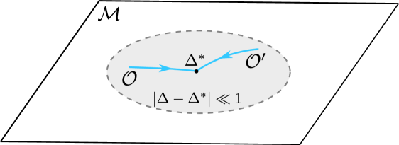
Figure 2.1: Different trajectories, corresponding to distinct marginal operators $\mathcal{O}$ and $\mathcal{O}^{\prime}$, in a neighborhood of the conformal manifold $\mathcal{M}$ leading to the same point with conformal dimension $\Delta^{\ast}$.

The idea behind our criterion to characterize whether a point is at (in)finite distance from a generic point in the interior of $\mathcal{M}$ is then the following: if one is able to obtain $C_{JJ\mathcal{O}}$ as a function of $\Delta_{\ell}$ close to the point under consideration, one can recover the behavior of the conformal dimension as a function of $t$ in that neighborhood using the evolution equation (2.16). As argued above, when the two-point function of $\mathcal{O}$ is chosen in an orthonormal basis, $t$ is then interpreted as the Zamolodchikov distance traveled along the trajectory specified by $\mathcal{O}$ itself. We can then use the behavior of $\Delta_{\ell}(t)$ as it approaches $\Delta_{\ell}^{\ast}$ to learn whether this point is at finite or infinite distance along the given trajectory.

Notice however that one can only obtain non-trivial information about the traveled distance when the conformal dimension varies along the trajectory. We hence need to pick a spin-$\ell$ operator whose conformal dimension is not fixed to a specific value over the whole conformal manifold. For instance, the energy-momentum tensor, conserved flavor currents, and protected BPS operators in supersymmetric theories have this property, and are therefore excluded from this analysis. We will thus assume that the higher-spin operators are conserved only at specific points or loci of the conformal manifold.

To illustrate this idea let us start with the most trivial—but also most generic— example, namely the case where the OPE combination can be considered constant in the neighborhood defined by $\Delta^{\ast}_{\ell}$: $C_{JJ\mathcal{O}}\to C_{JJ\mathcal{O}}^{*}\neq 0$ as $\Delta_{\ell}\to\Delta_{\ell}^{*}$. Defining the change in conformal dimension as $\gamma_{\ell}$, the evolution equation (2.16) reduces to:

$$\frac{d\gamma_{\ell}}{dt}=-\,C_{JJ\mathcal{O}}^{\,*}+\mathcal{O}(\gamma_{\ell})\,,\qquad C_{JJ\mathcal{O}}^{\,*}=\text{const}\,,\qquad\gamma_{\ell}=\Delta_{\ell}-\Delta_{\ell}^{\ast}\,.$$ (2.17)

Therefore, the leading behavior in the change of conformal dimension is given simply as a linear approximation

$$\gamma_{\ell}(t)\simeq\gamma_{\ell}^{0}-C_{JJ\mathcal{O}}^{\,*}\,t\,,$$ (2.18)

where we have fixed the integration constant in terms of the deviation at the point where we put the origin of the trajectory, namely ${\gamma}_{\ell}(t=0)=\gamma_{\ell}^{0}$. Of course, this approximation is only valid when the deviation $\gamma_{\ell}(t)$ is sufficiently small.

We have therefore obtained the solution to equation (2.16) close to ${\gamma}_{\ell}=0$ when $C_{JJ\mathcal{O}}$ takes a non-zero value at this point. Importantly, the solution given in equation (2.18) reaches $\gamma_{\ell}=0$ for finite values of $t$. In other words, this point is at finite distance from the initial point $t=0$ along the trajectory defined by $\mathcal{O}$.

To summarize, we see that if at some point in the conformal manifold we have $C_{JJ\mathcal{O}}^{*}\neq 0$ for a given marginal operator $\mathcal{O}$, then we have found a trajectory reaching this point within finite distance. Furthermore, finding a single trajectory for which this is true is enough to imply that the point under consideration is a finite-distance point in the conformal manifold.

Let us now give an example for which the point is reached at infinite distance. If the OPE coefficients grows linearly with the deviation,

$$C_{JJ\mathcal{O}}({\gamma}_{\ell})\simeq\alpha_{\chi}\,{\gamma}_{\ell}\,,\qquad\gamma_{\ell}=\Delta_{\ell}-\Delta^{\ast}_{\ell}\,,$$ (2.19)

for some constant $\alpha_{\chi}>0$, the evolution equation discussed above is solved by an exponential. The behavior of the deviation as it reaches zero is of the form:

$${\gamma}_{\ell}={\gamma}_{\ell}^{0}\,e^{-\alpha_{\chi}\,t}\,,$$ (2.20)

with the integration constant again fixed by ${\gamma}_{\ell}(t=0)={\gamma}_{\ell}^{0}$. As $t$ is again interpreted as the distance in the conformal manifold, we have the case of a trajectory with the exponential behavior typical of the CFT Distance Conjecture, see equation (1.1). Note that ${\gamma}_{\ell}\to 0$ for $t\to\infty$ regardless of the point where we place $t=0$, which means that this point is at infinite distance along the trajectory defined by the marginal operator $\mathcal{O}$. However, this does not mean that we have an infinite-distance point. Indeed, it could be that $\mathcal{O}$ is associated with a highly-non-geodesic trajectory, but there exists another trajectory for which the point can be reached within a finite distance.

To characterize whether a point where the conformal dimension is given by $\Delta_{\ell}^{\ast}$ is reached at finite distance or not along certain trajectory, let us consider a general case where $C_{JJ\mathcal{O}}$ is parameterized by:

$$C_{JJ\mathcal{O}}({\gamma}_{\ell})\sim{\gamma}_{\ell}^{1+a}\qquad\text{ as }{\gamma}_{\ell}=\Delta_{\ell}-\Delta^{\ast}_{\ell}\to 0\,.$$ (2.21)

Close to the reference point, and up to subleading corrections, the deviation from $\Delta_{\ell}^{*}$ then behaves as:

$$t\sim\,\left\{\,\begin{aligned} \log\,{\gamma}_{\ell}\,,\quad&\text{if }a=0\,,\\ {\gamma}_{\ell}^{-a}\,,\quad&\text{if }a\neq 0\,.\\ \end{aligned}\right.$$ (2.22)

For the same reasons as above, $t$ measures the distance from the distance from an arbitrary point encoded in the integration constant. The case $a<0$ corresponds to a finite distance, while $a\geq 0$ is at infinite distance. For $a=0$ we have not only the critical case between finite and infinite distance, but also the one where the deviation ${\gamma}_{\ell}$ decreases exponentially fast with the distance, that is the one associated with the third part of the CFT Distance Conjecture explained in the introduction. This is depicted in Figure 2.2.

Once again, we stress that if $a\geq 0$, this does not mean that the point at $t=0$ is an infinite-distance point, but could be associated with a non-geodesic trajectory and reach the point in an seemingly infinite-distance fashion. In order to ensure that it is truly an infinite-distance point, we need to show that it is the case for any trajectory. Conversely, a marginal operator inducing a trajectory where a point is at finite distance is sufficient to imply it is a finite-distance point, albeit it is maybe not attained via the shortest path. We have therefore found the following criterion.

CFT Distance Criterion:

In a neighborhood of a point of a conformal manifold $\mathcal{M}$ where higher-spin operators have conformal dimension $\Delta_{\ell}^{\ast}$, the behavior of the OPE combination $C_{JJ\mathcal{O}}$ defined in equation (2.14) as $\gamma_{\ell}=\Delta_{\ell}-\Delta_{\ell}^{\ast}\to 0$ is sufficient to decide whether it is a:

• Finite-distance point:  $\exists\,\mathcal{O}\text{ such that }C_{JJ\mathcal{O}}\sim{\gamma}_{\ell}^{1+a}\text{ with }a<0\,,$

• Infinite-distance point:  $C_{JJ\mathcal{O}}\sim{\gamma}_{\ell}^{1+a}\text{ with }a\geq 0\ \forall\mathcal{O}\,.$

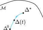
(a) Finite distance

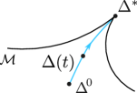
(b) Infinite distance

Figure 2.2: Two different trajectories associated with a marginal operator in the neighborhood of a point with dimension $\Delta^{*}$. If the OPE combination $C_{JJ\mathcal{O}}(t)$ remains approximately constant in the neighbourhood of the point, it is a finite-distance point. On the other hand, if $C_{JJ\mathcal{O}}\sim(\Delta-\Delta^{*})^{1+a}$ with $a\geq 0$, it is at infinite distance from any other point.

Note that this criterion does not depend on the precise nature of the operator $J_{\ell}$, and at no point did we assume a specific value of $\ell$, and should be valid for an conformal primary. To apply it, we only need an operator whose conformal dimension is not constant along the whole trajectory. Therefore, any operator for which this reasoning is applicable should give us the same answer. In particular, there cannot be an operator placing a point at finite distance while another predicts an infinite-distance behavior. This implies non-trivial relations between three-point functions of the form $\langle J_{\ell}J_{\ell}\mathcal{O}\rangle$ and the possible marginal operators for the conformal manifold to make sense as a metric space.

In this section, we have discussed how to differentiate between finite- and infinite-distance points of the conformal manifold, which typically requires understanding the behavior of $C_{JJ\mathcal{O}}$ close to that point for one or potentially even all marginal operators of the theory, an information that may be challenging to access in general. Despite this hurdle, we can draw an interesting observation: any point where $C_{JJ\mathcal{O}}$ is non-vanishing for any marginal operator is a finite-distance point. Conversely, a vanishing OPE combination is a necessary, albeit not sufficient, condition to have an infinite-distance point.

3 Higher-Spin Points are at Infinite Distance

Having a criterion to decide whether a point of the conformal manifold $\mathcal{M}$ is at infinite distance, we now apply the procedure described in the previous section to higher-spin (HS) points. There, (part) of the HS operators become conserved currents and the conformal group enhances to a larger, infinite-dimensional higher-spin symmetry.

In order to apply the CFT Distance Criterion to show that HS points are at infinite distance, we will assume that a given HS operator is never conserved everywhere in the conformal manifold, as this can happen only if it is part of a free subsector that is completely decoupled from the rest of the theory at all points of $\mathcal{M}$. Moreover, following the discussion at the end of the previous section, it is in principle enough to show that HS points are at infinite distance for an operator with e.g. spin $\ell=4$; there is indeed always a spin-four conserved current at any HS point [21, 22, 23, 24, 25]. While we could in principle set $\ell=4$ from now on, we will keep the spin arbitrary and specialize to the spin-four case for illustrative purposes.

3.1 Conservation Laws and Higher-Spin Correlators

At the HS point, the anomalous dimension of the higher-spin operator vanish and its conformal dimension saturates the unitarity bound for spin-$\ell$ operators: $\Delta_{\ell}=d-2+\ell$. As is well known in Conformal Field Theory, when this happens the associated conformal multiplet develops a null state corresponding to a conservation condition:

$$\partial\cdot J_{\ell}=\partial^{\mu}J_{\ell,\,\mu\nu_{1}\dots\mu_{\ell}}\,\xi^{\nu_{2}}\dots\xi^{\nu_{\ell}}=0\,.$$ (3.1)

This identity can be used to constrain correlators involving these conserved currents, as their divergences have to vanish up to contact terms. We will often refer to this as the current-conservation condition, and it will allow us to reduce the number of conformal structures that can appear in a given correlator. Starting with general type-$(\ell_{1},\ell_{2},\ell_{3})$ correlators and taking the divergence with respect to a HS operator, the current conservation conditions will impose constraints on its OPE coefficients. An important observation is that the null states associated with the divergence of conserved currents transform as spin-$(\ell-1)$ conformal primaries, see e.g. reference [99]. The current-conservation condition of a type-$(\ell_{1},\ell_{2},\ell_{3})$ correlator with respect to the first current is therefore equivalent to the vanishing of a type-$(\ell_{1}-1,\ell_{2},\ell_{3})$ three-point function. As was already realized in reference [21], since both the type-$(\ell_{1},\ell_{2},\ell_{3})$ and type-$(\ell_{1}-1,\ell_{2},\ell_{3})$ correlators can be written in terms of the same building blocks, see Section 2.1, we can instead write the divergence as a differential operator acting on the space of these building blocks. This considerably simplifies an otherwise rather cumbersome computation. The precise form of this operator can be found in reference [103], and we use it for cases of interest in Appendix A.

As already mentioned in Section 2.1, we note that parity-even and -odd structures do not mix in the current-conservation condition, as divergences preserve parity. To verify this, one can observe that the spin changes by one when taking the divergence, and that spin-$\ell$ operators acquires a sign $(-1)^{\ell}$ under parity. This—together with the fact that parity-odd structures do not contribute to equation (2.16)—allows us to ignore all allowed parity-odd $(d=3)$-structures for our purposes.

By Noether’s theorem, the HS conserved currents also have associated conserved charges by integrating them over a codimension-one surface $\Sigma$. Note that, contrary to the usual flavor charges, higher-spin charges have spin and we again use polarization vectors to contract the extra-indices. We then obtain a formal one-form that can be used to construct the charge:

$$Q_{\ell}(\xi)=\int_{\Sigma}\check{J}_{\ell}(\xi)\,,\qquad\check{J}_{\ell}(\xi)=J_{\ell,\,\mu\nu_{1}\dots\nu_{\ell-1}}\,\xi^{\nu_{1}}\dots\xi^{\nu_{\ell-1}}dx^{\mu}\,.$$ (3.2)

While the textbook approach to conserved charges involves integrating over the $(d-1)$ space coordinates, the usefulness of more general surfaces and induced topological properties of the charges have long been recognized, and have recently come in full force in the context of higher-form symmetries [104]. Note however that the charges $Q_{\ell}(\Sigma,\xi)$ have spin $\ell-1$ and act on (possibly-spinning) local operators and the currents transform in $\ell$-symmetric-traceless representations of the Lorentz group. While they do generalize the notion of ordinary spin-one flavor charges, they do not correspond to the type of generalized symmetries discussed in reference [104], which act on extended objects and the involved currents transform in anti-symmetric spacetime representations.

The conserved charges can be also used to constrain correlators involving HS conserved currents. Indeed, when inserted in a correlator, we must take into account contact terms—that is, contributions at coincident points:

$$\left<(\partial\cdot J_{\ell})(y,\xi)\Phi_{1}(x_{1})\cdots\Phi_{n}(x_{n})\right>\propto\sum_{k=1}^{n}\delta(y-x_{k})\left<\Phi_{1}(x_{1})\cdots[Q(\xi),\Phi_{k}(x_{k})]\cdots\Phi_{n}(x_{n})\right>\,,$$ (3.3)

up to a constant related to normalization, and the operators $\Phi_{n}$ are possibly spinning. Integrating over a $d$-dimensional submanifold of spacetime containing only a single position $x_{k}$, we can therefore select a given commutator and reduce the number of operators appearing in the correlator. On the other hand, using Stokes’ theorem on the LHS of equation (3.3), we can integrate the current, understood as a formal one-form as in equation (3.2), over the codimension-one surface $\Sigma$ bounding the submanifold. The charges are of course topological and we can deform the surface as long we are not crossing over another point, in which case we must take into account the appropriate commutator. We will refer to this as the integrated Ward identity and it will allow us to relate the OPE coefficients in a given correlator through properties of the HS algebra we review below.

Given the conserved charges, there is a further set of identities that one can impose on correlators to constrain not only their OPE coefficients but also how the charges can act on different operators. These are particularly interesting, since they allow us to impose the coexistence of HS symmetry with other ingredients of the theory like, e.g. the presence of the energy-momentum tensor. In fact, these constraints were crucial for the original derivation of the theorems relating HS points to free theories [21, 22, 23, 24, 25]. Following reference [21], we will call them charge-conservation identities. Given a set of operators, the idea is to consider the correlator of their commutator with $Q_{\ell}$. Since the conserved charge must annihilate the vacuum, this correlator must vanish. This is:

$$0=\left<[Q_{\ell}(\xi),\Phi_{1}(x_{1})\cdots\Phi(x_{n})]\right>=\sum_{k=1}^{n}\left<\Phi_{1}(x_{1})\cdots[Q_{\ell}(\xi),\Phi_{k}(x_{k})]\cdots\Phi_{n}(x_{n})\right>\,.$$ (3.4)

This can also be obtained from equation (3.3) by integrating over the entire of spacetime or any other submanifold that does not have a boundary, and containing all the positions $x_{k}$. Using Stokes’ theorem, the result must vanish.

Using the HS algebra to further expand each commutator in equation (3.4) as a sum over operators appearing in the various HS multiplets, one can infer a set of constraints involving both the parameters controlling the action of $Q_{\ell}$ on the operators and their OPE coefficients. In what follows, we review some of the properties of the HS algebra, give an example of such a charge-conservation identity, and its consequences.

The commutation relations of the charges must close and generate the full higher-spin algebra. In general, the action of the charges on an operator of twist $\tau=\Delta-\ell$ will involve derivatives of the various fields falling inside the same higher-spin multiplet so that the total twist is conserved. Tracking the index structure of such commutation relations can however be cumbersome, and it is instead very convenient to focus on a particular spacetime direction in order to simplify the index structure. Following reference [21], we will work in light-cone coordinates:

$$ds^{2}=dx^{+}dx^{-}+\delta_{ij}dx^{i}dx^{j}\,,\qquad i,j=2,\dots,d-1\,,$$ (3.5)

and use polarization vectors forcing the indices to be in the $(x^{-})$-direction: $\xi^{\mu}=\delta^{\mu}_{-}$. To differentiate HS operators in this regime from those with arbitrary polarizations, written with uppercase letters, e.g. $J_{\ell}(x,\xi)$, we will use lowercase letters to indicate spinning operators whose indices all point in that direction. For instance:

$$j_{\ell}=J_{\ell,-\dots-}\,.$$ (3.6)

The charges are then defined in terms of the currents with the indices in that direction

$$Q_{\ell}=\int_{\Sigma}dx^{-}d^{d-2}x\;\;j_{\ell}(x)\,,$$ (3.7)

where now $\Sigma$ is taken as a “slab” of spacetime in the directions perpendicular to $x^{+}$. For simplicity, we will henceforth drop the dependence on the polarization of the charges whenever the context is clear: $Q_{\ell}(\delta^{\mu}_{-})=Q_{\ell}$.

First, since the charges have twist zero, each term appearing in commutators involving $Q_{\ell}$ and an operator $k_{\ell^{\prime}}$ of twist $\tau$ must also have twist $\tau$. Moreover, these can only involve twist-$\tau$ operators $k_{\ell^{\prime\prime}}$ with all indices in the minus direction as well as $x^{-}$-derivatives, $\partial=\frac{\partial}{\partial x^{-}}$. Due to this index structure, each derivative increases the spin by one but the twist remains unchanged. The most general formula for such a commutator is then:

$$[Q_{\ell},k_{\ell^{\prime}}]=\sum_{\ell^{\prime\prime}=\text{max}(\ell^{\prime}-\ell+1,0)}^{\ell+\ell^{\prime}-1}\eta_{\ell^{\prime\prime}}\,\partial^{\ell+\ell^{\prime}-1-\ell^{\prime\prime}}k_{\ell^{\prime\prime}}\,.\\$$ (3.8)

As discussed above, the coefficients $\eta_{\ell}$ can be constrained—together with correlators—using the charge-conservation identities, and lead to a number of useful relations [21, 22, 23, 24, 25]. The simplest example is obtained by acting with $Q_{\ell}$ on the two-point function $\left<k_{\ell^{\prime}}k_{\ell^{\prime\prime}}\right>$. From this, one can show that if $k_{\ell^{\prime\prime}}$ appears in $[Q_{\ell},k_{\ell^{\prime}}]$ then $k_{\ell^{\prime}}$ must appear in $[Q_{\ell},k_{\ell^{\prime\prime}}]$.

Moreover, since we consider local theories, there is a spin-two conserved current that generates conformal transformations, the energy-momentum tensor $T_{\mu\nu}$. Additional constraints can be obtained by specifically considering charge-conservation identities on correlators involving $t_{2}=T_{--}$, as they enable us to further constrain the appearance of a given operator in commutators given in equation (3.8). For instance, since $t_{2}$ is related to the dilatation operator and charges have conformal dimension $\ell-1$, $j_{\ell}$ must always appear in $[Q_{\ell},t_{2}]$. Then, using this fact and charge-conservation identities, one can further show that not all a priori possible conserved currents appear in $[Q_{\ell},t_{2}]$. When $\ell=4$, one finds that the most general form of the commutator is given by:

$$[Q_{4},t_{2}]=\alpha_{0}\,\partial^{5}j_{0}+\alpha_{1}\,\partial^{4}j_{1}+\alpha_{2}\,\partial^{3}j_{2}+\alpha_{3}\,\partial^{2}j_{3}+\alpha_{4}\,\partial j_{4}\,.$$ (3.9)

By the argument above, $j_{4}$ must appear in the commutator and thus $\alpha_{4}\neq 0$. Notice that we do not need to assume that the energy-momentum tensor $t_{2}$ is the unique spin-two conserved current. This is, $j_{2}$ is a generic spin-two conserved current, that can include contributions from both $t_{2}$, and possibly any additional spin-two conserved current. When $t_{2}$ is the unique spin-two conserved current, not all coefficients $\alpha_{\ell}$ with $\ell=0,\cdots,5$ are non-zero, and it is possible to show that $\alpha_{1}=0=\alpha_{3}$ [21].

Restricting the possible operators appearing the various commutators will prove very powerful. It will allow us to show that some of the three-point functions involving marginal operators must vanish, and consequently will be crucial to prove that HS point are at infinite distance.

3.2 Higher-Spin Conserved Currents and Marginal Operators

Following the CFT Distance Criterion discussed in Section 2.3, a necessary condition for a HS point to be at infinite distance is that the OPE combination must vanish for any marginal operator at this point: $C_{JJ\mathcal{O}}^{\text{HS}}=0$. We will thus now shift our focus to three-point functions $\left<J_{\ell}J_{\ell}\mathcal{O}\right>$. Our goal is therefore to show that these correlators are always trivial, regardless of the chosen marginal operator.

To do so, we will first use the current-conservation condition on this correlator. This will impose constraints on the various OPE coefficients, reducing the number of allowed conformal structure to a single one. By further using an integrated Ward identity, we will then show that the remaining a priori independent parameter must vanish.

Let us start by imposing conservation of the higher-spin currents, see equation (3.1), on this three-point function. Up to contact terms, we have:

$$\partial_{2}\cdot\left<J_{\ell}(x_{1})J_{\ell}(x_{2})\mathcal{O}(x_{3})\right>=\left<J_{\ell}(x_{1})(\partial\cdot J_{\ell})(x_{2})\mathcal{O}(x_{3})\right>=0\,,$$ (3.10)

where $\partial_{i}$ is understood as taking the divergence with respect to the operator located at $x_{i}$. As discussed in Section 3.1, the LHS can be conveniently evaluated using a differential operator in the space of building blocks $H$, $V_{1}$, and $V_{2}$. Its expression, as well as the result for this current-conservation condition, can be found in Appendix A. Here, we will simply give a qualitative description of the procedure needed to show that at the higher-spin point, this three-point function and the related OPE combination vanish.

As we have seen in Section 2.1, for a fixed value of $\ell$ there are $\ell+1$ independent type-$(\ell,\ell,0)$ conformal structures, as defined in equation (2.5). Taking the divergence as in equation (3.10) we then obtain a linear combination of conformal structures of type $(\ell,\ell-1,0)$. Since there are only $\ell$ such structures, demanding that the resulting three-point function vanish leads to a set of $\ell$ linear constraints on the $\ell+1$ OPE coefficients $C_{JJ\mathcal{O}}^{\,n}$. If these $\ell$ constraints are independent, we can express all the OPE coefficients in terms of a single one, and the solution takes the form:

$$C_{JJ\mathcal{O}}^{\,n}=v^{n}\,C_{JJ\mathcal{O}}^{\,\ell}\,,\qquad n=0,\dots,\ell\,,$$ (3.11)

where the components of the vector, denoted as $v^{n}\in\mathbb{R}$, are normalized such that $v^{\ell}=1$. This is found by showing that the current-conservation constraint in equation (3.10) can be viewed as a recursion relation in the space of OPE coefficients $C_{JJ\mathcal{O}}^{\,n}$. In general, solving this for arbitrary values of $\ell$ is difficult, but not particularly illuminating. It is on the other hand straightforward to do it on a case-by-case basis. For instance, when $\ell=4$ the coefficients are given by:

$$v^{n}=\left(\frac{-24}{(d-2)d(d+2)(d+6)}\,,\,\frac{48(d+3)}{(d-2)d(d+2)(d+6)}\,,\,\frac{72}{(d-2)d(d+6)}\,,\,\frac{-8(d+7)}{(d-2)(d+6)}\,,\,1\right)\,.$$ (3.12)

However, the specific values of $v^{n}$ will not be relevant for our analysis, only that the current-conservation constraint reduces the number of allowed structure from $(\ell+1)$ to only one. The details of this computation can be found in Appendix A.

To see the impact of this constraint on the conformal-perturbation-theory equations, let us write the OPE combination at the HS point after imposing the Ward identity (3.10):

$$C^{\text{HS}}_{JJ\mathcal{O}}=C_{JJ\mathcal{O}}^{\ell}\,\sum_{n=0}^{\ell}w_{n}v^{n}\,.$$ (3.13)

While one could hope that $\sum_{n=0}^{\ell}w_{n}v^{n}=0$, directly showing that $C_{JJ\mathcal{O}}^{\text{HS}}=0$, this is unfortunately generically not the case. We have checked this explicitly for $4\leq\ell\leq 10$ in any dimension by using the expression of coefficients $w_{n}$, given in equation (2.15), and those of $v^{n}$, obtained by solving the recursive relation obtained in Appendix A. In fact, it is hard to believe that there is a given spin $\ell$ for which it vanishes for any dimension. The strategy is then to further show that the yet-undetermined OPE coefficient $C_{JJ\mathcal{O}}^{\,\ell}$ has to vanish. Doing so will establish that $C^{\text{HS}}_{JJ\mathcal{O}}=0$—as expected—in a way that does not depend on the precise values of $v^{n}$ and $w_{n}$.

To show that this is the case, we now turn to the integrated Ward identity, which allows us to reduce the correlator to a two-point function. Fixing the coordinates $x_{2}$ and $x_{3}$, we can use a version of the Ward identity (3.3) applied to our case and integrate the current over a submanifold only containing $x_{2}$, and we obtain:

$$\int_{\Sigma}\left\langle\check{J}_{\ell}(x_{1},\xi_{1})J_{\ell}(x_{2},\xi_{2})\mathcal{O}(x_{3})\right\rangle\propto\left\langle\left[Q_{\ell}(\xi_{1}),J_{\ell}(x_{2},\xi_{2})\right]\mathcal{O}(x_{3})\right\rangle\,.$$ (3.14)

The codimension one surface $\Sigma$ is the boundary of the submanifold containing $x_{2}$. The integral is then performed with respect to the first HS conserved current $\check{J}_{\ell}$, where the first index is in direction normal to $\Sigma$, see equation (3.2).

As discussed above, the commutator of an operator with a conserved charge must involve only operators of the same twist, and in this case they must therefore all have $\tau=d-2$. However marginal operators have twist $\tau=d$, and as a consequence there cannot be any operator appearing in the commutator so that the two-point function on the RHS of equation (3.14) does not vanish, and we conclude that:

$$\left\langle\left[Q_{\ell},J_{\ell}(x_{2})\right]\mathcal{O}(x_{3})\right\rangle=0\,.$$ (3.15)

By consistency, the integral on the LHS of equation (3.14) must also vanish. If we choose $\Sigma$ such that it picks the component of $\check{J}$ in the direction of $\xi_{1}$, we can then expand the correlator in terms of the conformal structures, and using equation (3.11), we can factor out the so-far-undetermined coefficient $C_{JJ\mathcal{O}}^{\,\ell}$ to obtain:

$$\int_{\Sigma}\left\langle J_{\ell}(x_{1},\xi_{1})J_{\ell}(x_{2},\xi_{2})\mathcal{O}(x_{3})\right\rangle=C_{JJ\mathcal{O}}^{\,\ell}\int_{\Sigma}\left(\sum_{n=0}^{\ell}v^{n}\,\Theta_{n}(x_{i};\xi_{1},\xi_{2})\right)\overset{!}{=}0\,.$$ (3.16)

If we can find polarization vectors $\xi_{1},\xi_{2}$ so that the integral gives a non-zero result, the constraint coming from the integrated Ward identity can only be satisfied if $C_{JJ\mathcal{O}}^{\,\ell}=0$, as desired. In Appendix B, we show explicitly that the integral indeed does not vanish for a particular choice of polarization vectors. We therefore conclude that at any HS point and for any marginal operator $\mathcal{O}$, the three-point function $\left\langle J_{\ell}J_{\ell}\mathcal{O}\right\rangle$ is trivial, and by extension so is the OPE combination relevant to the CFT Distance Criterion:

$$C^{\text{HS}}_{JJ\mathcal{O}}=0\,.$$ (3.17)

This result is in the end not too surprising. In fact, it is known that when the two spins are different, the OPE coefficients vanish, see e.g. references [98, 105]. For equal spin however, the conservation condition is not enough to come to this conclusion, as one must use the integrated Ward identity.

For a theory of 4d free vectors, which include $\mathcal{N}=4$ super-Yang–Mills in the free-field limit, this result can be obtained from a direct computation by decomposing the field-strength into (anti-)self dual components $F=F_{+}+F_{-}$. The only non-vanishing two-point function of the field-strength is $\langle F_{+}F_{-}\rangle$, and the HS currents and marginal operators can be written as [106]:

$$J_{\ell}\sim F_{+}\partial^{\ell}F_{-}\,,\qquad\mathcal{O}\sim F_{+}F_{+}+F_{-}F_{-}\,,$$ (3.18)

where we have been very cavalier with the index structure. By Wick’s theorem, the relevant three-point functions then directly vanish:

$$\langle(F_{+}\partial^{\ell}F_{-})\,(F_{+}\partial^{\ell}F_{-})\,(F_{+}F_{+})\rangle=0=\langle(F_{+}\partial^{\ell}F_{-})\,(F_{+}\partial^{\ell}F_{-})\,(F_{-}F_{-})\rangle\,.$$ (3.19)

As advertised, we have therefore found that the OPE combination always vanishes at any HS point, $C^{\text{HS}}_{JJ\mathcal{O}}=0$. We stress that this result is not sensible to the actual numerology of the coefficients $w_{n}$ and $v^{n}$, but is rather a consequence of the properties of the higher-spin symmetry.

This result shows that higher-spin points are not in the regular finite-distance class for which $C_{JJ\mathcal{O}}\neq 0$. However, the fact that the OPE combination must vanish is a necessary but not sufficient condition to show that these points are at infinite distance. To complete the proof, we require information about their neighborhood, and what happens when the higher-spin symmetry is weakly broken.

3.3 Weakly-broken Higher-Spin Symmetries

In this section we move slightly away from the higher-spin point. This is, we assume that the higher-spin symmetry is weakly broken by a small parameter $g$ (related, but not to be confused with the marginal coupling $t$ used in conformal perturbation theory). This is, for the divergence of the higher-spin operators we have:

$$\partial\cdot J_{\ell}=g\,K_{\ell-1}\,.$$ (3.20)

Here, we have introduced an operator $K_{\ell-1}$ controlling the higher-spin symmetry breaking. This operator is a primary of twist $d$ and spin $\ell-1$ only at the HS point, i.e., at leading order in $g\to 0$ [97, 107, 108]. In fact, the two multiplets recombine into a larger multiplet with primary $J_{\ell}$—which is no longer conserved due to the anomalous dimension—and $K_{\ell-1}$ is a mere descendant of the would-be current away from the higher-spin point [109]. We take this operator to be in an orthonormal basis, also at leading order in this limit. This in turn fixes the definition of the higher-spin symmetry breaking parameter $g$ via equation (3.20).

Breaking the HS symmetry, the decoupled sector is not free anymore, and $K_{\ell-1}$ can be thought of as specifying the type of interactions that are turned on. However, we will not assume that the CFT data enjoys an expansion in powers of $g$ around the HS point. The reason is that $g$ is not necessarily the coupling constant of those interactions. For instance, it could a priori happen that $\partial\cdot J_{\ell}$ vanishes at tree level, and the breaking occurs only at higher-loop orders. In this case, the CFT data would generically have an expansion in fractional powers of $g$. Here, we will only assume that the CFT data remains finite as the HS point is approached. This is closely related to the normalization of operators such as $J_{\ell}$, $K_{\ell-1}$, and $\mathcal{O}$. Normalizations in which we allow the two-point functions to diverge as $g\to 0$ can lead to similar, unphysical, divergences in the three-point functions. Nevertheless, this cannot happen when operators are properly normalized. In this case the three-point-function coefficients are physical and should remain finite in any bona fide CFT like those associated with HS points of the conformal manifold.

As pioneered in reference [97], let us now take the double divergence of the two-point function of two higher-spin operators, and use the broken Ward identity defined in equation (3.20):

$$\partial_{1}\partial_{2}\cdot\left\langle J_{\ell}(x_{1})J_{\ell}(x_{2})\right\rangle=g^{2}\left\langle K_{\ell-1}(x_{1})K_{\ell-1}(x_{2})\right\rangle\,.$$ (3.21)

The LHS of this expression can be directly computed using the form of the two-point function as an expansion in terms of the conformal structures, see equation (2.2). For small anomalous dimensions, $\gamma_{\ell}=\tau_{\ell}-(d-2)\ll 1$, it is at leading order proportional to a spin-$(\ell-1)$ two-point function [105, 110]. Since $K_{\ell-1}$ is a conformal primary for $g\to 0$, the RHS is also proportional to the two-point function of a spin-$(\ell-1)$ conformal primary in that limit. We then conclude that, at leading order, the anomalous dimension is given by:

$$\gamma_{\ell}\sim g^{2}\,,\qquad\text{as }g\to 0\,,$$ (3.22)

where we are ignoring numerical prefactors whose precise values can be found in references [105, 110]. In this way we see that the first contribution to the anomalous dimension of the higher-spin operators always appears at order $g^{2}$ in the higher-spin symmetry-breaking parameter. This result is sometimes referred to as Anselmi’s trick, who first used the broken Ward identity to simplify the computations of the anomalous dimensions of the Konishi current and other spinning operators for four-dimensional $\mathcal{N}=4$ super-Yang–Mills theory[97].

We can apply similar arguments to the three-point function $\langle J_{\ell}J_{\ell}\mathcal{O}\rangle$. Let us first take the divergence with respect to the second higher-spin operator and use equation (3.20):

$$\partial_{2}\cdot\left\langle J_{\ell}(x_{1})J_{\ell}(x_{2})\mathcal{O}(x_{3})\right\rangle=g\left\langle J_{\ell}(x_{1})K_{\ell-1}(x_{2})\mathcal{O}(x_{3})\right\rangle\,.$$ (3.23)

As for the two-point function, at leading order the divergence of the currents matches with the correlator of spinning primaries. Something similar happens for the three-point function in the RHS, and we see that the leading-order corrections to the current-conservation condition, which led to (3.11), are controlled by the behavior of $\left\langle J_{\ell}K_{\ell-1}\mathcal{O}\right\rangle$ close to the HS point.

Similarly, a weakly-broken version of the integrated Ward identity goes as follows: because of equation (3.20), the charges defined in equation (3.2) are no longer conserved, and as a result their correlators depend on the codimension-one surface $\Sigma$. One can however define the action of quasi-conserved charges on a given operator as the result of the integral when the surface $\Sigma$ enclosing its position shrinks to zero size [108]. This action is constrained by twist conservation as it was the case when the symmetry was exactly preserved. By virtue of Stokes’ theorem, one then gets integrated Ward identities similar to the conserved case, but with an extra contribution from the correlator where $J_{\ell}$ has been replaced by $\partial\cdot J_{\ell}=gK_{\ell-1}$, integrated over the volume enclosed by $\Sigma$. As happens for the current-conservation condition, the leading-order correction to the integrated Ward identity for $\left<J_{\ell}J_{\ell}\mathcal{O}\right>$ is again controlled by the behavior of $\left\langle J_{\ell}K_{\ell-1}\mathcal{O}\right\rangle$ close to the HS point.

Putting these two results together and taking into account equation (3.17), we get that for a weakly-broken HS symmetry we have

$$C_{JJ\mathcal{O}}\sim g\,C_{JK\mathcal{O}}\qquad\text{ as }g\to 0\,,$$ (3.24)

where $C_{JK\mathcal{O}}$ is a certain linear combination of the OPE coefficients appearing in $\left<J_{\ell}K_{\ell-1}\mathcal{O}\right>$ as defined in equation (2.6).

If $C_{JK\mathcal{O}}$ is non-vanishing at the HS point, we see that the OPE combination behaves as $C_{JJ\mathcal{O}}\sim g$ when $g\to 0$. Using equation (3.22), this would mean that at leading order, we would have $C_{JJ\mathcal{O}}\sim\gamma^{1/2}$. Following the CFT Distance Criterion discussed in Section 2.3, this would result in HS points being at finite distance with respect to the trajectory defined by the marginal operator $\mathcal{O}$. For the first part of the CFT Distance conjecture to be true, the OPE combination $C_{JK\mathcal{O}}$ must always be trivial at the HS point. We now show this is indeed the case.

3.3.1 The Correlator $\langle J_{\ell}K_{\ell-1}\mathcal{O}\rangle$ at the HS Point

To show that at the higher-spin point the correlator $\langle J_{\ell}K_{\ell-1}\mathcal{O}\rangle$ vanishes, we will go through a similar procedure to the one we used for the three-point function $\langle J_{\ell}J_{\ell}\mathcal{O}\rangle$, and begin with the current-conservation condition. We now have to take the divergence of a type-$(\ell,\ell-1,0)$ correlator with respect to the first operator, from which we obtain a three-point function of type-$(\ell-1,\ell-1,0)$. Using that $K_{\ell-1}$ is a conformal primary at this point, and as explained in Section 2.1, both correlators involve $\ell$ independent conformal structures. As before, this enable us to find an homogeneous system of $\ell$ linear constraints for $\ell$ variables $C_{JK\mathcal{O}}^{n}$.

If all the equations were independent, one would automatically get that $C_{JK\mathcal{O}}^{n}=0$. Unfortunately, we have checked that the system is not closed for $2\leq\ell\leq 10$ and for any $d$. In general, we therefore expect that this happens for any spin and any number of spacetime dimensions. Despite this, we show in the Appendix A that the constraints can always be used to fix most of the coefficients, and we get a similar result as for $C_{JJ\mathcal{O}}^{n}$:

$$C_{JK\mathcal{O}}^{n}=\tilde{v}^{n}\,C_{JK\mathcal{O}}^{\ell-1}\,,\qquad n=0,\dots,\ell-1\,,$$ (3.25)

where the components of the vector, denoted by $\tilde{v}^{n}\in\mathbb{R}$, are normalized such that $\tilde{v}^{\ell-1}=1$. In appendix A, we argue that, similarly to what we have done for the case of $\left<J_{\ell}J_{\ell}\mathcal{O}\right>$ above, the current-conservation constraint imposes a recursion relation in the space of OPE coefficients $C_{JK\mathcal{O}}^{n}$. We have not found a closed-form expression for the coefficients $\tilde{v}^{n}$, but they can easily be solved for a given spin programmatically. For instance, for $\ell=4$ it is straightforward to check that the solution is given by:

$$\tilde{v}^{n}=\left(\frac{-24}{(d-2)d(d+2)}\,,\,\frac{36}{(d-2)d}\,,\,\frac{-12}{d-2}\,,\,1\right)\,.$$ (3.26)

Once again, the particular values of $\tilde{v}^{n}$ is not important, only that that the current-conservation condition fixes all the coefficients but one.

To show that this remaining coefficient is in fact trivial, we again need to impose the integrated Ward identity. Starting with the analogue of equation (3.3), we integrate the current over a manifold enclosing the point $x_{2}$ with boundary $\Sigma$, and we obtain:

$$\int_{\Sigma}\left\langle\check{J}_{\ell}(x_{1},\xi_{1})K_{\ell-1}(x_{2},\xi_{2})\mathcal{O}(x_{3})\right\rangle\propto\left\langle\left[Q_{\ell}(\xi_{1}),K_{\ell-1}(x_{2},\xi_{2})\right]\mathcal{O}(x_{3})\right\rangle\,,$$ (3.27)

and $\check{J}_{\ell}$ is the current with the first index in the direction normal to the surface. As we did for the three-point function $\left\langle J_{\ell}J_{\ell}\mathcal{O}\right\rangle$, taking $\Sigma$ to pick the $\xi_{1}$-direction, the LHS can be expanded in terms of the conformal structures. Taking into account equation (3.25), we then have:

$$\int_{\Sigma}\left\langle J_{\ell}(x_{1},\xi_{1})K_{\ell-1}(x_{2},\xi_{2})\mathcal{O}(x_{3})\right\rangle=C_{JK\mathcal{O}}^{\ell-1}\int_{\Sigma}\left(\sum_{n=0}^{\ell}\tilde{v}^{n}\widetilde{\Theta}_{n}(x_{i};\xi_{1},\xi_{2})\right)\,.$$ (3.28)

As discussed in Appendix B, the same choice of polarization vector and surface we used for $\left\langle J_{\ell}J_{\ell}\mathcal{O}\right\rangle$ again lead to a non-vanishing integral. However, a crucial difference is that the commutator in equation (3.27) is not trivial in this case. Indeed, due to twist conservation, only twist $\tau=d$ operators can appear in the commutator from the relation given in equation (3.8). Since marginal operators also have twist $d$, it can in principle be contained in the commutator, and we cannot conclude that the three-point function $\left\langle J_{\ell}K_{\ell-1}\mathcal{O}\right\rangle$ vanishes as in the previous subsection.

To do so, we need to invoke an ingredient that we have not used so far, namely the presence of the energy-momentum tensor. Indeed, assuming a local CFT is what makes the CFT distance conjecture part of the holographic Swampland Program, as it implies the presence of dynamical gravity in the bulk. Note that here we do not assume a weakly-coupled gravity dual, and will only use the interplay of the energy-momentum tensor with the higher-spin algebra. As alluded to in Section 3.1, it can be used to constrain the operators appearing in the commutators involving higher-spin charges [21].

In particular, our goal is to show that $\left<J_{\ell}K_{\ell-1}\mathcal{O}\right>\neq 0$ is inconsistent with a charge-conservation identity. We will achieve this by considering the action of $Q_{\ell}$ on the three-point function $\left\langle T_{2}K_{\ell-1}\mathcal{O}\right\rangle$:

$$\left<\left[Q_{\ell},t_{2}k_{\ell-1}\mathcal{O}\right]\right>=\left<\left[Q_{\ell},t_{2}\right]k_{\ell-1}\mathcal{O}\right>+\left<t_{2}\left[Q_{\ell},k_{\ell-1}\right]\mathcal{O}\right>+\left<t_{2}k_{\ell-1}\left[Q_{\ell},\mathcal{O}\right]\right>=0\,,$$ (3.29)

which can be understood as integrating equation (3.3) over all of spacetime. We recall that we use the notation—explained in Section 3.1—where lowercase operators indicate that the indices are all taken in the $x^{-}$-direction, e.g. $t_{2}=T_{--}$ for the energy-momentum tensor, and the HS charges are defined as in equation (3.7).

Let us first discuss the action of one of these charges on the energy-momentum tensor:

$$\left[Q_{\ell},t_{2}\right]=\sum_{s=0}^{\ell}\alpha_{s}\,\partial^{\ell+1-s}j_{s}\,,$$ (3.30)

Recall that $\partial$ denotes the partial derivative with respect to the $x^{-}$-direction. Even though it is allowed by twist and spin conservation, notice that we have not included $j_{\ell+1}$. The reason is that, were it to appear in the commutator then $Q_{\ell}$ would not be translation invariant [21]. Note that we are not assuming uniqueness of the spin two conserved current, in general $j_{2}$ could contain contributions from both the energy-momentum tensor $t_{2}$, and any other spin-two current.

The action of $Q_{\ell}$ on $k_{\ell-1}$ and $\mathcal{O}$ leads to similar expressions, see equation (3.8):

$$\begin{split}\left[Q_{\ell},k_{\ell-1}\right]&=\sum_{s=0}^{2\ell-2}\eta_{s}\,\partial^{2\ell-2-s}k_{s}^{\prime}\,,\\ \left[Q_{\ell},\mathcal{O}\right]&=\sum_{s=0}^{\ell-1}\beta_{s}\,\partial^{\ell-1-s}k_{s}^{\prime}\,.\end{split}$$ (3.31)

The primed operators $k_{s}^{\prime}$ are there to remind us that they might be different from unprimed operators $k_{\ell-1}$ we have considered so far. Furthermore, the twist-$d$ scalar operators $k_{0}^{\prime}$ might be different from the marginal operator $\mathcal{O}$ we started with.

Plugging these commutators into equation (3.29), we then obtain:

$$\sum_{s=0}^{\ell}\alpha_{s}\,\partial^{\ell+1-s}_{1}\left<j_{s}k_{\ell-1}\mathcal{O}\right>+\sum_{s=0}^{2\ell-2}\eta_{s}\,\partial^{2\ell-2-s}_{2}\left<t_{2}k^{\prime}_{s}\mathcal{O}\right>+\sum_{s=0}^{\ell-1}\beta_{s}\,\partial^{\ell-1-s}_{3}\left<t_{2}k_{\ell-1}k_{s}^{\prime}\right>=0\,,$$ (3.32)

where $\partial_{i}$ denotes the partial $x^{-}$-derivative with respect to the position of the $i$-th operator. Notice that the first sum contains a term with $\alpha_{\ell}\neq 0$ and $\left<j_{\ell}k_{\ell-1}\mathcal{O}\right>$, if the charge-conservation identity imposes that this term must vanish, then we obtain the desired result.

Performing this analysis for general spin $\ell$ is quite involved, but it becomes more manageable for $\ell=4$. In this case we have:

$$\sum_{s=0}^{4}\alpha_{s}\,\partial^{5-s}_{1}\left<j_{s}k_{3}\mathcal{O}\right>+\sum_{s=0}^{6}\eta_{s}\,\partial^{6-s}_{2}\left<t_{2}k^{\prime}_{s}\mathcal{O}\right>+\sum_{s=0}^{3}\beta_{s}\,\partial^{3-s}_{3}\left<t_{2}k_{3}k_{s}^{\prime}\right>=0\,.$$ (3.33)

We then have to analyze correlators of type $\left<J_{s}K_{3}\mathcal{O}\right>$, $\left<T_{2}K_{s}\mathcal{O}\right>$ and $\left<T_{2}K_{3}K_{s}\right>$. Using the current-conservation condition and integrated Ward identities, we conclude that:

$$\begin{split}\left<J_{s}K_{3}\mathcal{O}\right>&=0\qquad\text{for }s=2,3\,;\\ \left<T_{2}K_{s}\mathcal{O}\right>&=0\qquad\text{for }s=1,\dots,6\,;\\ \left<T_{2}K_{3}K_{s}\right>&=0\qquad\text{for }s=0\,.\end{split}$$ (3.34)

This can be shown as we did for $\left<J_{\ell}J_{\ell}\mathcal{O}\right>$: the current conservation condition reduces the number of independent OPE coefficients to one, and the integrated Ward identity then imposes that the remaining OPE coefficient must vanish. For the case $\left<T_{2}K_{1}\mathcal{O}\right>$ it is crucial to use that $T_{2}$ is the energy-momentum tensor. Only in this case $Q_{2}$ is the charge generating translations in the minus direction, $Q_{2}=P_{-}$, which guarantees that even though allowed by twist conservation, $K_{1}$ does not appear in $[Q_{2},\mathcal{O}]$. The results for the current-conservation conditions and the integrals for the integrated Ward identities can be found in appendices A and B.

Using this, the charge-conservation condition reduces to

$$\begin{split}0=\,&\alpha_{0}\,\partial^{5}_{1}\left<j_{s}k_{0}\mathcal{O}\right>+\alpha_{1}\,\partial^{4}_{1}\left<j_{1}k_{3}\mathcal{O}\right>+\alpha_{4}\,\partial_{1}\left<j_{4}k_{3}\mathcal{O}\right>+\,\eta_{0}\,\partial^{6}_{2}\left<t_{2}k^{\prime}_{0}\mathcal{O}\right>\\ &+\beta_{1}\,\partial^{2}_{3}\left<t_{2}k_{3}k_{1}^{\prime}\right>+\beta_{2}\,\partial_{3}\left<t_{2}k_{3}k_{2}^{\prime}\right>+\beta_{3}\,\left<t_{2}k_{3}k_{3}^{\prime}\right>\,.\end{split}$$ (3.35)

The last three terms are more complicated to analyze, since the current-conservation condition allows for more than one conformal structure. However, including them in the charge-conservation condition becomes more manageable when coordinates are taken in the light-cone plane, $x_{i}=(x_{i}^{-},x_{i}^{+},\mathbf{0})$, since only one linear combination of the conformal structures of these correlators contributes in this case. Moreover, the spacetime dependence of all the conformal structures simplify drastically. Imposing this charge-conservation condition for any $x_{i}^{-}$ and $x_{i}^{+}$, we find that there is no solution if $\left<j_{4}k_{3}\mathcal{O}\right>\neq 0$, thus arriving to the desired result:

$$\left<J_{4}K_{3}\mathcal{O}\right>=0\,.$$ (3.36)

This concludes the analysis of the correlator $\left<J_{\ell}K_{\ell-1}\mathcal{O}\right>$ at the HS point. At least for the case $\ell=4$, we have been able to show that this correlator must vanish for any marginal operator $\mathcal{O}$. This in turn implies that

$$C_{JK\mathcal{O}}^{\text{HS}}=0\,,$$ (3.37)

as we wanted. Following the same procedure as for $\ell=4$, we expect the same result to hold for $\ell>4$. In fact, this has to be the case for any other HS conserved current coexisting with $J_{4}$ to generate the higher-spin algebra, otherwise the conformal manifold would stop making sense as a metric space. We come back to this point in the next section.

3.4 Infinite Distance and Exponentially Conserved Currents

In this section, we have so far shown that by using various properties of the higher-spin algebra, two of the three-point functions involving marginal operators and a HS current must always be trivial at the HS point:

$$\text{HS point:}\qquad\langle J_{\ell}J_{\ell}\mathcal{O}\rangle=0=\langle J_{\ell}K_{\ell-1}\mathcal{O}\rangle\,.$$ (3.38)

Following the CFT Distance Criterion defined in Section 2.3, the first term is a necessary condition for HS points to be at infinite distance in the conformal manifold. On the other hand, from the discussion around equation (3.23), the fact that second vanishes forbids contributions to the OPE combination $C_{JJ\mathcal{O}}$ at linear order in the parameter $g$ for a weakly-broken HS symmetry.

By the same token, one can reach a similar conclusion for $C_{JK\mathcal{O}}(g)$ away from the HS point. Taking the divergence with respect to $J_{\ell}$ and using equation (3.20) we have

$$\partial_{1}\cdot\left<J_{\ell}(x_{1})K_{\ell-1}(x_{2})\mathcal{O}(x_{3})\right>=g\left<K_{\ell-1}(x_{1})K_{\ell-1}(x_{2})\mathcal{O}(x_{3})\right>\,.$$ (3.39)

The leading order correction to the current-conservation condition for $\left<J_{\ell}K_{\ell-1}\mathcal{O}\right>$ is controlled by $\left<K_{\ell-1}K_{\ell-1}\mathcal{O}\right>$ at the HS point. The same observation can be reached for the leading correction to the integrated Ward identity and the charge-conservation condition [108]. Similarly to what we obtained in the previous section, and taking into account equation (3.37), we now have

$$C_{JK\mathcal{O}}\sim g\,C_{KK\mathcal{O}}\qquad\text{ as }g\to 0\,,$$ (3.40)

where $C_{KK\mathcal{O}}$ is again a certain linear combination of the OPE coefficients appearing in $\left<K_{\ell-1}K_{\ell-1}\mathcal{O}\right>$.

Since both $K_{\ell}$ and $\mathcal{O}$ are assumed to be in an orthonormal basis, the correlator $\left<K_{\ell-1}K_{\ell-1}\mathcal{O}\right>$ cannot blow up as $g\to 0$—see the discussion below equation (3.20). In general, we therefore have

$$\left<K_{\ell-1}K_{\ell-1}\mathcal{O}\right>\sim g^{2a}\qquad\text{ with }a\geq 0\,\text{ as }g\to 0\,.$$ (3.41)

By this equation, we mean that the $\ell$ OPE coefficients of this correlator, $C_{KKO}^{n}$, have this behavior as $g\to 0$. Combining this with equations (3.24) and (3.40), we have

$$C_{JJ\mathcal{O}}\sim g^{2(1+a)}\qquad\text{ with }a\geq 0\,\text{ as }g\to 0\,$$ (3.42)

for the OPE combination controlling the conformal-perturbation-theory equation (2.16). Given the behavior of the anomalous dimension in equation (3.22), we finally reach the conclusion

$$C_{JJ\mathcal{O}}\sim\gamma_{\ell}^{1+a}\qquad\text{ with }a\geq 0\,\text{ as }\gamma_{\ell}\to 0\,.$$ (3.43)

Since we have made no assumption on the marginal operator $\mathcal{O}$, this behavior is independent of the deformation away from the higher-spin point, and is precisely the CFT Distance Criterion for an infinite-distance point in the conformal manifold, as explained in Section 2.3. Furthermore, we have not made any assumptions on the operators $J_{\ell}$ either, apart from the fact that they become conserved at the HS point. This then shows that for local CFTs in any dimension, the first part of the CFT Distance Conjecture is correct:

all higher-spin points are at infinite distance in the conformal manifold.

Strictly speaking, in Section 3.3 we have only proven this for spin-four currents. However, as discussed below the CFT Distance Criterion in Section 2.3, it is enough to show that a single higher-spin current places the HS point at infinite distance in the conformal manifold. The rest of the tower should behave accordingly, and we must also have $\left<J_{\ell}K_{\ell-1}\mathcal{O}\right>=0$ at the HS point for any other current. Furthermore, since there is always a spin-four conserved current generating the higher-spin algebra [21, 22, 23, 24, 25], the case $\ell=4$ suffices to establish that any HS point is at infinite distance.

It is also interesting to elaborate more on the condition for the higher-spin currents to become conserved exponentially with the distance. This would be the case if $a=0$ in equation (3.43). In other words, having an exponentially conserved HS current with the distance as the HS point is approached is linked to having:

$$\left<K_{\ell-1}K_{\ell-1}\mathcal{O}\right>_{\text{HS}}\neq 0\,.$$ (3.44)

In particular, this does not mean that all the OPE coefficients $C_{KK\mathcal{O}}^{n}$ are non-vanishing as the HS point. We only need to require this for the OPE combination $C_{KK\mathcal{O}}$ controlling the order $g^{2}$ correction to $C_{JJ\mathcal{O}}$. It is intriguing that the condition for the exponential behavior precisely involves the last correction to $C_{JJ\mathcal{O}}$ that can be addressed using Anselmi’s trick, i.e. the weakly-broken Ward identity (3.20).

Having $\left<K_{\ell-1}K_{\ell-1}\mathcal{O}\right>\neq 0$ at the infinite distance HS point might seem a bit puzzling. Indeed, one of the corollaries of the CFT Distance Criterion is that having an operator with non-vanishing three point function with $\mathcal{O}$ is generically enough to imply that the point is at finite distance. However, let us recall that $K_{\ell-1}$ is not a conformal primary outside the HS point, while the CFT Distance Criterion assumes this for the operator under consideration, and equation (2.16) therefore does not apply to the descendant $K_{\ell-1}$. The analogous equation, obtainable through conformal perturbation theory applied to this non-primary operator, should be such that the behavior of $C_{KK\mathcal{O}}$ close to the HS point must place it at infinite distance. In fact, in our case this is guaranteed by the fact that, when going away from the HS point, the current and $K_{\ell-1}$ recombine into a larger multiplet, and their behavior as we approach the free point must be related.

If equation (3.44) is satisfied, then the exponential decay rate $\alpha_{\chi}^{(\ell)}$ appearing in equation (1.1) is controlled by the OPE combination $C_{KKO}$ at the HS point. Schematically, we have:

$$\alpha_{\chi}^{(\ell)}\sim\left<K_{\ell-1}K_{\ell-1}\mathcal{O}\right>_{\text{HS}}\,,$$ (3.45)

where the numerical coefficients and the OPE combination, $C_{KK\mathcal{O}}$, can be fixed by the weakly-broken HS symmetry constraints. In fact, this result can be brought into a more suggestive form. Taking an orthonormal basis for the set of marginal operators $\mathcal{O}_{i}$ and generalizing the evolution equation (2.16) we have

$$\frac{\partial_{i}\gamma_{\ell}}{\gamma_{\ell}}\sim\left<K_{\ell-1}K_{\ell-1}\mathcal{O}_{i}\right>_{\text{HS}}\,.$$ (3.46)

An orthonormal basis for the marginal operators corresponds to an orthonormal basis for the tangent bundle of the conformal manifold. Therefore, equation (3.46) gives the components of what is defined as the scalar charge-to-mass ratio vector used for the convex-hull formulation of the Swampland Distance Conjecture [111]. This equation is then telling us that, close to the HS point, this information is encoded in this particular three-point function.

Showing the condition given in equation (3.44) for a single spin, e.g. $\ell=4$, is not enough to show an exponential behavior for all off them. There is a priori nothing wrong with having an infinite-distance point for which the different HS currents become conserved at different rates along a given trajectory in the conformal manifold. The only thing that is required by consistency of the conformal manifold as a metric space is that $\gamma_{\ell}(t)\to 0$ as $t\to\infty$ for all of them.

Despite this, there might be a way of translating the result for a single spin to the rest of the tower. The idea is to exploit a relation that we have not discussed yet. Even though the HS symmetry-breaking parameter $g$ is not the same as the distance $t$ in the conformal manifold, they are related. Indeed, having shown the exponential behavior for the anomalous dimension of a given spin $\ell$, and using equation (3.22) we get the relation:

$$g_{\ell}^{2}\sim e^{-\alpha_{\chi}^{(\ell)}\,t}\qquad\text{ as }t\to\infty\,.$$ (3.47)

Here we have added a subscript $\ell$ to the HS symmetry breaking parameter to make clear that a priori one could expect the parameters to be different for the breaking of the conservation condition of different HS operators. However, coming back to the underlying picture of introducing an interaction with a small coupling, we indeed expect them to be related in a power-like fashion. This is, we expect each of these conservation conditions to be broken at a given loop order. Note however that this could be avoided if the conservation condition for some HS currents is broken only by non-perturbative effects.

Following this reasoning, the exponential behavior for a given spin would carry over to the others, even though the exponential decay rate might still depend on $\ell$. It would be interesting to show that, as it happens for super-Yang–Mills theories, all the HS conservation conditions are broken at the same order, i.e, $g_{\ell}=g$. In fact, it seems plausible that this is imposed by consistency of the HS symmetry breaking, since this symmetry relates the different HS currents. If this is case, one would not only conclude that it is enough to show the exponential behavior for a single spin, but also that the exponential rate $\alpha_{\chi}$ does not depend on $\ell$ and one has a full tower of HS currents becoming exponentially conserved at the same rate.

4 Flavor Enhancements at (In)Finite Distances

In the previous section, we have used properties of the higher-spin algebra to show that HS points are at infinite distance. Although we focused on higher-spin currents, many aspect of this machinery turns out to also be valid for $\ell=1$. In the conformal manifold, this corresponds to regimes where a new conserved flavor current appears in the spectrum. These special points need not automatically be associated with higher-spin points, nor with infinite distances. A classical family of examples is $(\mathcal{N}=1)$-preserving deformations of four-dimensional $\mathcal{N}=4$ super-Yang–Mills [3], where new R-symmetry currents are accompanied with extra supercharges, see e.g. reference [112] for an analysis of the possible multiplet recombination rules. These enhancements are associated with superpotential deformations, and are at finite distance [80].

On the other hand, not all flavor-enhancement point are at finite distance. In $\mathcal{N}=2$ four-dimensional theories, representation-theoretic arguments show that spin-one would-be-conserved current are in the same long multiplet as would-be higher-spin currents. At threshold, the long multiplet then splits into (at least) two short multiplets and both the flavor and HS currents become conserved [113, 114, 112]. The flavor-enhancement points are therefore also higher-spin points, and always at infinite-distance in the conformal manifold from the results of the previous section. This is related to the decomposability conjecture [114], stating that non-trivial $\mathcal{N}=2$ conformal manifolds can only be obtained by performing a conformal gauging of the flavor symmetry of isolated theories. The decoupled sector is then made out of the spectrum of free vector multiplets.

One can then ask whether a similar fate awaits more general cases, where we only assume that there exist a neighborhood of the flavor-enhancement point such that the broken Ward identity is valid:

$$\partial_{\mu}J^{\mu}=g\,K_{0}\,.$$ (4.1)

At the point where $g=0$, $K_{0}$ is a scalar conformal primary with $\Delta=d$, but develops an anomalous dimension elsewhere. The two operators $J_{1}$ and $K_{0}$ recombine into a larger multiplet away from that point, where $K_{0}$ is a conformal descendant [109].

The first step of our argument required us to show that, when $g=0$, the OPE combination vanishes: $C_{JJ\mathcal{O}}=0$. The current-conservation condition applied to the correlator $\langle J_{1}J_{1}\mathcal{O}\rangle$ again fixes the two OPE coefficents to be proportional to one another:

$$C_{JJ\mathcal{O}}^{0}=\frac{1}{d}C_{JJ\mathcal{O}}^{1}\,.$$ (4.2)

But, contrary to cases where $\ell>1$, we cannot use the integrated Ward identity to conclude that the remaining coefficient must vanish. Indeed, as shown in Appendix A for the choice of surface $\Sigma$ discussed in Section 3.2, the integral vanishes and we cannot conclude that $C_{JJ\mathcal{O}}=0$ in this case.

It is nevertheless tempting to assume that the OPE combination should vanish at the flavor-enhancement point. Were it not the case, taking $\gamma^{0}_{\ell=1}=0$ as the reference point in equation (2.18), the anomalous dimension would become negative, $\gamma\simeq-C_{JJ\mathcal{O}}\,t<0$, and violate unitarity bounds. Since it is at least in principle possible to deform away from the flavor-enhancement point in the directions associated with both $\pm\mathcal{O}$, corresponding to the two directions away from the point along the line parameterized by $t$, one of them always lead to a violation of unitarity. A possible escape could be that somehow conformal perturbation theory breaks down in that direction, leaving us with only a semi-infinite critical line.

For now, let us thus assume that the OPE combination indeed vanishes: $C_{JJ\mathcal{O}}=0$. We are then led to consider the correlator $\langle J_{1}K_{0}\mathcal{O}\rangle$ at the point $g=0$. The current-conservation condition is automatically satisfied, and using the integrated Ward identity we obtain:

$$\int_{\Sigma}dx^{\mu}\,\langle J_{1,\mu}(x_{1})K_{0}(x_{2})\mathcal{O}(x_{3})\rangle\propto\langle[Q_{1},K_{0}(x_{2})]\mathcal{O}(x_{3})\rangle\,.$$ (4.3)

The integral on the LHS can be expanded in terms of the single type-$(1,0,0)$ conformal structure, and, as shown in Appendix B, the result is non-vanishing in any dimension.

Whether the OPE combination $C_{JK\mathcal{O}}$ is trivial—and by extension whether the flavor-enhancement point is at infinite distance via the CFT Distance Criterion—is therefore decided by the commutator $[Q_{1},K_{0}]$. If any of the marginal operators belong to the same multiplet as the twist-$d$ operator, $[Q_{1},K_{0}]\sim\mathcal{O}$, then the two-point function on the RHS of equation (4.3) is non-vanishing and $C_{JK\mathcal{O}}\neq 0$. The associated limiting point is then at finite distance. If on the other hand none of the marginal operators share a multiplet with $K_{0}$, the RHS of equation (4.3) is trivial and the flavor-enhancement point is at infinite distance—provided that $C_{JJ\mathcal{O}}=0$ at that point, as discussed above.

Let us note that the charge-conservation identity applied in Section 3.3 for the case of HS symmetry does not help in this case. Precisely for $\ell=1$, $j_{1}$ cannot appear in $[Q_{1},j_{2}]$, since $Q_{1}$ has vanishing conformal dimension. This is the usual statement that the energy-momentum tensor should be invariant under any global symmetry. We thus have to set $\alpha_{1}=0$ in equation (3.32) and the correlator of interest $\left<j_{1}K_{0}\mathcal{O}\right>$ does not appear in the charge-conservation condition.

In addition, the unitarity argument that we presented in favor of $C_{JJ\mathcal{O}}=0$ at the flavor-enhancement point does not work either. If we have $C_{JK\mathcal{O}}\neq 0$, then the behavior of the OPE combination is given by $C_{JJ\mathcal{O}}\sim g\sim\sqrt{\gamma_{1}}$, which leads to $\gamma_{1}\sim t^{2}$ upon using equation (2.16). This is at finite distance, but the anomalous dimension is not linear with the Zamolodchikov distance $t$, as it is the case for $C_{JJ\mathcal{O}}\neq 0$ at the flavor-enhancement point. Therefore, this would not lead to a violation of the unitarity bound in any of the two directions departing from the flavor-enhancement point along the line parametrized by $t$.

The condition we have found for the flavor-enhancement point to be at finite distance is of course very intuitive. It is equivalent to the statement that the marginal operators are charged under the symmetry. We could have alternatively chosen another integration domain so that equation (4.3) is written in terms of the charges acting on $\mathcal{O}$, which would have led us to the condition $[Q_{1},\mathcal{O}]\sim K_{0}$. For a deformation—marginal or not—to preserve a symmetry the associated operator must be in the singlet representation. In the context of R-symmetry, this was used to classify possible supersymmetry-preserving deformations in various dimensions [3, 8, 5]. In the example of $\mathcal{N}=4$ super-Yang Mills described above, the marginal operators are indeed charged under the extra symmetry, and this explains why they are at finite distance.

Conversely, if none of the marginal operators are charged under the flavor symmetry, it cannot be explicitly broken or restored. One would then expect that in the conformal manifold this point can only be reached asymptotically and is therefore at infinite distance. This is consistent with a flavor symmetry emerging as a sector becomes free, namely a higher-spin point. It then begs the question of the possible existence of other flavor-enhancement points at infinite distance. According to the second part of the CFT Distance Conjecture, this cannot be the case, and an emerging flavor symmetry must be accompanied by a free sector. While in 4d $\mathcal{N}=2$ SCFTs this is enforced by the superconformal algebra [113, 114, 112], we are not aware of similar arguments in more general cases. The study of spin-one operators and their behavior in the conformal manifold therefore seem like an avenue to test the rest of the CFT Distance Conjecture.

5 Conclusions

A weakly-broken higher-spin symmetry imposes remarkably strong constraints on the form of the correlators. By studying conformal perturbations close to higher-spin points, we have harnessed it to show that these points must always be at infinite Zamolodchikov distance in the conformal manifold, establishing part of the CFT Distance Conjecture.

In particular, we have combined two different types of perturbations. First, we have used conformal perturbation theory to find a criterion which can be used to decide whether a point is at infinite distance, given in terms of the behavior of certain OPE coefficients near the point of the conformal manifold under consideration. Furthermore, we have also utilized the broken Ward identities appearing close to points where there is a symmetry enhancement. Through Anselmi’s trick, this enabled us to find the leading behavior of the these coefficients without needing to involve the details of a particular microscopic description.

Combining these two techniques have shown to be powerful as they were sufficient to show that the first part of the CFT Distance Conjecture is indeed correct. One can then wonder about the possibility of proving the converse, namely that infinite-distance points can only be accompanied with a higher-spin enhancement, and whether the machinery discussed here can be deployed to prove the rest of the conjecture. One would need to show that the absence of the HS current at such points lead to an inconsistency, perhaps violating the assumptions of local unitary CFTs. We expect that the CFT Distance Criterion could help in this endeavour. We note that efforts have already been spent in that direction, as it was recently shown using inversion formulae that singularities of the curvature of the Zamolodchikov metric can only occur in the presence of higher-spin currents [20], or if the CFT develops a continuum.

Concerning the third part of the conjecture—stating that the anomalous dimension vanishes exponentially fast with the distance at higher-spin points—an analysis connected to our results using conservation identities seems promising. We have indeed shown that this exponential behavior happens along a given trajectory if $C_{KK\mathcal{O}}^{\text{HS}}\neq 0$. Therefore, the third part of the conjecture holds if there is always a marginal operator $\mathcal{O}$ such that this OPE combination is non-vanishing at the HS point. Note that the presence of at least one such operators with this property is enough. The presence of other marginal operators for which $C_{KK\mathcal{O}}\to 0$ as the HS point is approached would correspond to non-geodesic trajectories that avoid an exponential behavior, and that are known to exist in the context of the Swampland Distance Conjecture [45, 111]. It is furthermore remarkable that this condition only requires information about the HS point, and one could hope that this follows from the higher-spin algebra. However, the operators $K_{\ell-1}$ are not as constrained as the related conserved currents $J_{\ell}$. A study of the associated correlators is then more difficult without considering specific models, and we leave such analyses for future works.

We stress again that, while the evidence for the conjecture has originated from limiting behaviors of SCFTs, our arguments have not relied on supersymmetry, and are valid across dimensions. It would however be interesting to investigate if we can uncover new properties of conformal manifolds by imposing this additional structure. Part of our analysis might be simplified, and connect constraints of different spins. There are also examples of conformal manifolds that are compact [10], and all conformal manifolds of three-dimensional CFTs have been conjectured to be so as well [80]. It would be interesting to check ad absurdum if assuming the presence of a broken Ward identity for the higher-spin symmetry in those cases leads to inconsistencies. In the same vein, while we have not assumed the presence of supercharges, we have not tackled the question of non-supersymmetric conformal manifolds, and only required the presence of marginal operators regardless of the mechanism protecting them against quantum corrections. While there have been hints of possible cases [115], their existence is not yet settled.

We have furthermore seen that for spin-one cases, some of the arguments we have used fail, particularly to show that $C_{JJ\mathcal{O}}^{\text{HS}}=0$, a key ingredient of our analysis. Similarly, we could not reach the conclusion $C_{JK\mathcal{O}}^{\text{HS}}=0$. This is not a flaw but a feature, since flavor enhancements are known to happen at both finite and infinite distance in the conformal manifold. Our analysis leads to simple and intuitive conditions diagnosing which case occurs. One can then ask whether the condition for having a flavor-enhancement point at infinite distance would imply that it comes with additional HS conserved currents. This seems to be a promising scenario for making progress towards the second part of the CFT Distance Conjecture.

Our work falls into the broader context of the holographic Swampland Program, and provides a step forward in the understanding of the constraints imposed by quantum gravity through the AdS/CFT correspondence. While we have not discussed the gravity duals of the local CFTs, our results have implications for theories of quantum gravity in AdS backgrounds [79, 80]. A striking feature of our analysis is that it does not assume that the families of CFTs are holographic, but only that they have an energy-momentum tensor. This signals that the Swampland Distance Conjecture could hold beyond weakly-coupled Einstein gravity. On more general grounds, one may wonder what constraints must be imposed to conformal theories to address other Swampland conjectures.

Furthermore, our results lend more validity to the physical intuition that Vasiliev-type gravity—with infinitely many massless HS fields—should be infinitely far away from Einstein gravity, i.e. they should not be connected by small deformations [80]. They are moreover in agreement with the Emergence proposal—see e.g. references [116, 117, 44, 46, 30, 118, 119, 120, 121] for works in this direction—which implies that points for which an infinite number of weakly-coupled fields become massless should always be at infinite distance. It would also be interesting to connect with the results that were obtained in references [88, 89], by further studying how the correlators factorize, particularly when only a subsector of the theory becomes free. In addition, further exploring conformal manifolds of local CFTs (possibly with a weakly-coupled gravity dual) and their possible HS points might shed some light on the fate of the Emergent String Conjecture [39] beyond flat backgrounds, see reference [79] for an analysis of this conjecture applied to examples of AdS/CFT dual pairs in string theory.

Finally, this work is but an example of possible synergies between conformal theories and the Swampland Program. The Distance Conjectures have been developed by studying the constraints on field theories imposed by quantum gravity, but have been applied to conformal manifold independently of this origin. Other Swampland conjectures might therefore serve as a guide for other questions on the field-theory side, and motivate particular answers. On the other hand, conformal techniques have proven to lead to very rigorous results, and could allow one to establish more thoroughly—or disprove—some of the more speculative part of the program, and go beyond the current lamppost.

Acknowledgements

We thank A. Antunes, S. Komatsu, M. Montero, K. Papadodimas, F. Tellander, A. Uranga, I. Valenzuela, T. Weigand and A. Zhiboedov for helpful discussions and comments on early versions of the manuscript, as well as E. Skvortsov for helpful correspondence. J.C. would like to thank the Department of Physics at Harvard University and the Instituto de Física Teórica in Madrid for hospitality during early stages of this work. F.B. is supported by the German Research Foundation through a German-Israeli Project Cooperation (DIP) grant “Holography and the Swampland”, by the Swiss National Science Foundation (SNSF), grant number P400P2_194341, and in part by the Deutsche Forschungsgemeinschaft under Germany’s Excellence Strategy EXC 2121 Quantum Universe 390833306. The work by J.C. is partially supported by the Spanish Agencia Estatal de Investigacion through the grant “IFT Centro de Excelencia Severo Ochoa CEX2020-001007-S, the grants PGC2018-095976-B-C21 and PID2021-123017NB-I00, funded by MCIN/AEI/10.13039/ 501100011033, by ERDF A way of making Europe, and the FPU grant no. FPU17/04181 from the Spanish Ministry of Education.

Appendix A Current-Conservation Conditions

In Section 3, we discuss the various constraints the higher-spin algebra imposes on correlators. In particular, the Ward identity $\partial\cdot J_{\ell}=0$ can be used to relate some of the OPE coefficients of a given three-point function involving $J_{\ell}$. As pointed out in references [21, 103], taking the divergence of the three-point functions can be rephrased in terms of a differential operator acting in the space of the building blocks constituting the conformal structures. For the correlators we are considering, there are only three building blocks for the conformal structures defined in equations (2.5) and (2.7): $H_{12}$, $V_{1}$ and $V_{2}$ (their expressions as function of the coordinates and polarization vectors are shown in equation (B.1)).

In all generality, the expression of the differential operator for type-$(\ell_{1},\ell_{2},\ell_{3})$ correlators depends on all six building blocks, and was given in reference [103], whose conventions we follow. For our purpose, we will always consider three-point functions involving a marginal operator, $\ell_{3}=0$, which simplifies considerably the expressions we will have to deal with. We will successively treat the two cases at hand, namely $\langle J_{\ell}J_{\ell}\mathcal{O}\rangle$ and $\langle J_{\ell}K_{\ell-1}\mathcal{O}\rangle$. For clarity, we reproduce here the conformal structure in both cases, using that $J_{\ell}$ has twist $d-2$, while $K_{\ell-1}$ and $\mathcal{O}$ have twist $d$:

$$\Theta_{n} =\frac{\mathcal{P}_{n}}{|x_{12}|^{d-4}|x_{13}|^{d}|x_{23}|^{d}}\,,\qquad \mathcal{P}_{n} =H_{12}^{\ell-n}(V_{1}V_{2})^{n}\,,$$ (A.1)

$$\widetilde{\Theta}_{n} =\frac{\widetilde{\mathcal{P}}_{n}}{|x_{12}|^{d-2}|x_{13}|^{d-2}|x_{23}|^{d+2}}\,,\qquad \widetilde{\mathcal{P}}_{n} =H_{12}^{\ell-n-1}V_{1}^{n+1}V_{2}^{n}\,.$$

We have denoted the numerators $\mathcal{P}$ and $\tilde{\mathcal{P}}$, as these are the quantities on which the differential operator discussed above is applied.

Current Conservation for $\langle J_{\ell}J_{\ell}\mathcal{O}\rangle$

In this case, the conservation equation leads to the following constraint:

$$\langle J_{\ell}(x_{1},\xi_{1})(\partial\cdot J_{\ell})(x_{2},\xi_{2})\mathcal{O}(x_{3})\rangle=0\quad\Leftrightarrow\quad\mathcal{D}_{2}\,\langle J_{\ell}(x_{1},\xi_{1})J_{\ell}(x_{2},\xi_{2})\mathcal{O}(x_{3})\rangle=0\,.$$ (A.2)

where the differential operator, understood as acting on the second current, reduces from the original expression [103] to:

$$\mathcal{D}_{2}=\frac{\mathcal{D}_{2}^{(3)}}{d-2}+\mathcal{D}_{2}^{(2)}+(d-2)\mathcal{D}_{2}^{(1)}-2\left(\frac{\delta\mathcal{D}_{2}^{(2)}}{d-2}+\delta\mathcal{D}_{2}^{(1)}\right)\,,$$ (A.3)

with

$$\begin{split}\mathcal{D}_{2}^{(1)}&=V_{1}\,\partial_{H_{12}}\,,\\ \mathcal{D}_{2}^{(2)}&=2H_{12}V_{1}\,\partial_{H_{12}}^{2}+V_{1}\,\partial_{V_{1}}\partial_{V_{2}}+\left(H_{12}+2V_{1}V_{2}\right)\,\partial_{V_{2}}\partial_{H_{12}}\,,\\ \mathcal{D}_{2}^{(3)}&=2H_{12}\left(H_{12}+2V_{1}V_{2}\right)\,\partial_{V_{2}}\partial_{H_{12}}^{2}+\left(H_{12}+2V_{1}V_{2}\right)\,\partial_{V_{1}}\partial_{V_{2}}^{2}\,,\\ \delta\mathcal{D}_{2}^{(1)}&=\partial_{V_{2}}-V_{1}\,\partial_{H_{12}}\,,\\ \delta\mathcal{D}_{2}^{(2)}&=V_{2}\,\partial_{V_{2}}^{2}+2H_{12}\,\partial_{V_{2}}\partial_{H_{12}}-2V_{1}H_{12}\,\partial_{H_{12}}^{2}\,.\\ \end{split}$$ (A.4)

Note that we can safely ignore all terms involving building blocks that do not appear in the type-$(\ell,\ell,0)$ conformal structures. Furthermore, in reference [103], the operator is defined as acting on the first operator. To get to the above equation, we have exchanged the indices $1\leftrightarrow 2$.

As explained in Section 3, this operator can then be applied to each of the conformal structures, $\Theta_{n}$. The differential operator is taking care of the contribution from the denominator by design, and we find the following relation for the numerator of a given structure:

$$\begin{split}(d-2)\mathcal{D}_{2}\mathcal{P}_{n}&=n^{2}(n-1)\,\widetilde{\mathcal{P}}_{n-2}\\ &+n\left[d(\ell-2)+2(3+\ell^{2}-2\ell(n+2)+2n^{2}+n)\right]\,\widetilde{\mathcal{P}}_{n-1}\\ &+(\ell-n)(d+2n)(d-4+2\ell-2n)\,\widetilde{\mathcal{P}}_{n}\,.\end{split}$$ (A.5)

As expected, all dependence on the building blocks can be written in terms of the numerator of the type-$(\ell,\ell-1,0)$ conformal structures $\widetilde{\Theta}_{n}$, see equation (A.1). We can then plug in those relations in the numerator of the three-point function $\langle J_{\ell}J_{\ell}\mathcal{O}\rangle$:

$$\mathcal{P}=\sum_{n=0}^{\ell}C_{JJ\mathcal{O}}^{\,n}\mathcal{P}_{n}\,.$$ (A.6)

After shifting the sums and a bit of algebra to simplify the expression, everything can be rewritten as a single sum:

$$\begin{split}(d-2)\mathcal{D}_{2}\mathcal{P}&=\sum_{n=0}^{\ell-1}\bigg{[}(n+2)^{2}(n+1)\,C_{JJ\mathcal{O}}^{n+2}\\ &+(n+1)\left[d(\ell-2)+2(6+\ell^{2}-2\ell(n+3)+2n^{2}+5n)\right]\,C_{JJ\mathcal{O}}^{n+1}\\ &+(\ell-n)(d+2n)(d-4+2\ell-2n)\,C_{JJ\mathcal{O}}^{n}\bigg{]}\,\widetilde{\mathcal{P}}_{n}\,,\end{split}$$ (A.7)

where we have defined $C_{JJ\mathcal{O}}^{\ell+1}=0$. Note that this is a boundary condition, as the OPE coefficient $C_{JJ\mathcal{O}}^{n}$ have a physical meaning only for $0\leq n\leq\ell$. The current conservation condition then imposes that the prefactors in front of each $\widetilde{\mathcal{P}}_{n}$ must all vanish, leading to a system of constraints:

$$A(n)\,C_{JJ\mathcal{O}}^{n+2}+B(n)\,C_{JJ\mathcal{O}}^{n+1}+D(n)\,C_{JJ\mathcal{O}}^{n}=0\,,\quad n=0,\dots,\ell-1\,,$$ (A.8)

where we have defined

$$\begin{split}A(n)&=(n+2)^{2}(n+1)\,,\\ B(n)&=(n+1)\left[d(\ell-2)+2(6+\ell^{2}-2\ell(n+3)+2n^{2}+5n)\right]\,,\\ D(n)&=(\ell-n)(d+2n)(d-4+2\ell-2n)\,,\end{split}$$ (A.9)

and one has to keep in mind the boundary condition:

$$C_{JJ\mathcal{O}}^{\ell+1}=0\,.$$ (A.10)

As discussed in the main text, this is a homogeneous system of $\ell$ equations for $\ell+1$ variables. For given $d>2$ and $\ell\geq 0$, one can check that $D(n)\neq 0$ for $0\leq n\leq\ell-1$, and we can rewrite this as:

$$C_{JJ\mathcal{O}}^{n}=-\frac{1}{D(n)}\left(A(n)\,C_{JJ\mathcal{O}}^{n+2}+B(n)\,C_{JJ\mathcal{O}}^{n+1}\right)\,,\quad n=0,\dots,\ell-1\,.$$ (A.11)

In this form, we clearly see that this is a recursion relation in the space of OPE coefficients $C_{JJ\mathcal{O}}^{n}$. Using $C^{\ell}_{JJ\mathcal{O}}$ and $C_{JJ\mathcal{O}}^{\ell+1}=0$ as initial conditions and starting from $n=\ell-1$, we can find any of the OPE coefficients as being proportional to $C^{\ell}_{JJ\mathcal{O}}$, and we indeed find the result given in equation (3.11).

Notice that since $A(n)\neq 0$ for $0\leq n\leq\ell-1$, we could instead have started with $n=0$ and solved the system in ascending order. However, in this way $C_{JJ\mathcal{O}}^{\ell+1}=0$ cannot be used as an initial condition. This will lead to solutions in terms of $C_{JJ\mathcal{O}}^{0}$ and $C_{JJ\mathcal{O}}^{1}$, plus the constraint imposed by the boundary condition $C_{JJ\mathcal{O}}^{\ell+1}=0$. As it is not guaranteed that the last constraint is non-trivial, we find it more convenient to write the solution in terms of $C_{JJ\mathcal{O}}^{n}$.

As advertised in Section 3, given the current conservation condition for $\langle J_{\ell}J_{\ell}\mathcal{O}\rangle$, we have shown that we can always write all the OPE coefficients $C_{JJ\mathcal{O}}^{n}$ in terms of $C_{JJ\mathcal{O}}^{\ell}$ as in equation (3.11). In other words, this condition reduces the number of allowed conformal structures from $\ell+1$ to only one. For arbitrary dimension and spin, we have not found a closed-form solution of the recursion relation. However, it can be easily solved for fixed values programmatically, see equations (4.2) and (3.12) for $\ell=1,4$.

Current Conservation for $\langle J_{\ell}K_{\ell-1}\mathcal{O}\rangle$

Imposing the divergence of the higher-spin current $J_{\ell}$ in the case of the three-point function $\left<J_{\ell}K_{\ell-1}\mathcal{O}\right>$ proceeds mutatis mutandis from that of $\langle J_{\ell}J_{\ell}\mathcal{O}\rangle$. The divergence is again translated into a differentiation in the space of building blocks:

$$\langle(\partial\cdot J_{\ell})(x_{1},\xi_{1})K_{\ell-1}(x_{2},\xi_{2})\mathcal{O}(x_{3})\rangle=0\quad\Leftrightarrow\quad\mathcal{D}_{1}\,\langle J_{\ell}(x_{1},\xi_{1})K_{\ell-1}(x_{2},\xi_{2})\mathcal{O}(x_{3})\rangle=0$$ (A.12)

The differential operator applied to the first operator is now simpler than in the previous case, and given by [103]:

$$\mathcal{D}_{1}=\frac{\mathcal{D}_{1}^{(3)}}{d-2}+\mathcal{D}_{1}^{(2)}+(d-2)\mathcal{D}_{1}^{(1)}\,,$$ (A.13)

where we have defined each component as:

$$\begin{split}\mathcal{D}_{1}^{(1)}&=V_{2}\,\partial_{H_{12}}\,,\\ \mathcal{D}_{1}^{(2)}&=2H_{12}V_{2}\,\partial_{H_{12}}^{2}+V_{2}\,\partial_{V_{1}}\partial_{V_{2}}+\left(H_{12}+2V_{1}V_{2}\right)\,\partial_{V_{1}}\partial_{H_{12}}\,,\\ \mathcal{D}_{1}^{(3)}&=2H_{12}\left(H_{12}+2V_{1}V_{2}\right)\,\partial_{V_{1}}\partial_{H_{12}}^{2}+\left(H_{12}+2V_{1}V_{2}\right)\,\partial_{V_{1}}^{2}\partial_{V_{2}}\,.\\ \end{split}$$ (A.14)

Once again, following the procedure explained in Section 3, this operator is applied to the numerator of the correlator. The numerators $\widetilde{\mathcal{P}}_{n}$ of the type-$(\ell,\ell-1,0)$ conformal structure $\widetilde{\Theta}_{n}$ then satisfies the following relation:

$$\begin{split}(d-2)\mathcal{D}_{1}\widetilde{\mathcal{P}}_{n}&=(n+1)n^{2}\,\mathcal{P}_{n-1}\\ &+(n+1)\left[(\ell-1)(d+2\ell-6)-(4\ell-6)n+4n^{2}\right]\,\mathcal{P}_{n}\\ &+(\ell-1-n)(d+2n)(d-6+2\ell-2n)\,\mathcal{P}_{n+1}\,.\end{split}$$ (A.15)

As expected, all dependence on the building blocks can be written in terms of the numerator of type-$(\ell-1,\ell-1,0)$ conformal structures $P_{n}$, see equation (A.1). Plugging these relations into the numerator of the full three-point function $\left<J_{\ell}K_{\ell-1}\mathcal{O}\right>$:

$$\widetilde{\mathcal{P}}=\sum_{n=0}^{\ell-1}C_{JK\mathcal{O}}^{n}\widetilde{\mathcal{P}}_{n}\,,$$ (A.16)

we then have

$$\begin{split}(d-2)\mathcal{D}_{1}\widetilde{\mathcal{P}}&=\sum_{n=0}^{\ell-1}(n+1)n^{2}\,C_{JK\mathcal{O}}^{n}\mathcal{P}_{n-1}\\ &+\sum_{n=0}^{\ell-1}(n+1)\left[(\ell-1)(d+2\ell-6)-(4\ell-6)n+4n^{2}\right]\,C_{JK\mathcal{O}}^{n}\mathcal{P}_{n}\\ &+\sum_{n=0}^{\ell-1}(\ell-1-n)(d+2n)(d-6+2\ell-2n)\,C_{JK\mathcal{O}}^{n}\mathcal{P}_{n+1}\,.\end{split}$$ (A.17)

Shifting the sums, we can rewrite the sums in terms of summands containing only $\mathcal{P}_{n}$ if we impose $C_{JK\mathcal{O}}^{-1}=0=C_{JK\mathcal{O}}^{\ell}$. Note that this is not a constraint on the OPE coefficients, as for type-$(\ell,\ell-1,0)$ correlators $C_{JK\mathcal{O}}^{n}$ has a physical meaning only for $0\leq n\leq\ell-1$. After a few algebraic manipulations, we find:

$$\begin{split}(d-2)\mathcal{D}_{1}\widetilde{\mathcal{P}}&=\sum_{n=0}^{\ell-1}\bigg{[}(n+2)(n+1)^{2}\,C_{JK\mathcal{O}}^{n+1}\\ &+(n+1)\left[(\ell-1)(d+2\ell-6)-(4\ell-6)n+4n^{2}\right]\,C_{JK\mathcal{O}}^{n}\\ &+(\ell-n)(d-2+2n)(d-4+2\ell-2n)\,C_{JK\mathcal{O}}^{n-1}\bigg{]}\mathcal{P}_{n}\,.\end{split}$$ (A.18)

The current-conservation condition then imposes that the prefactors of each $\mathcal{P}_{n}$ to vanish, and we once more obtain:

$$\tilde{A}(n)\,C_{JK\mathcal{O}}^{n+1}+\tilde{B}(n)\,C_{JK\mathcal{O}}^{n}+\tilde{D}(n)\,C_{JK\mathcal{O}}^{n-1}=0\,,\quad n=0,\dots,\ell-1\,,$$ (A.19)

where we have defined

$$\begin{split}\tilde{A}(n)&=(n+2)(n+1)^{2}\,,\\ \tilde{B}(n)&=(n+1)\left[(\ell-1)(d+2\ell-6)-(4\ell-6)n+4n^{2}\right]\,,\\ \tilde{D}(n)&=(\ell-n)(d-2+2n)(d-4+2\ell-2n)\,,\end{split}$$ (A.20)

and we impose the following boundary conditions:

$$C_{JK\mathcal{O}}^{-1}=0=C_{JK\mathcal{O}}^{\ell}\,.$$ (A.21)

Taking into account the constraints, this is a homogeneous system of $\ell$ equations for $\ell$ variables. If it is closed, all the OPE coefficients must vanish. However, in practice we find that only $\ell-1$ equations are independent, and the OPE coefficients $C_{JK\mathcal{O}}^{n}$ are all related to each other. Dealing with this system of equations for arbitrary $\ell$ is however tedious because the spin controls the number of equations and variables, but it can easily be solved for fixed values of the dimension and spin through computational means.

Despite this, in what follows we show that in the worst-case scenario, this system of equations always allows us to fix all OPE coefficients in terms of $C_{JK\mathcal{O}}^{\ell-1}$. Conversely, in the best-case scenario the system is closed and we further have $C_{JK\mathcal{O}}^{\ell-1}=0$—we have checked that, unfortunately, this only happens in a few sporadic cases.

Given $d>2$ and $\ell\geq 0$, one can check that $\tilde{D}(n)\neq 0$ for $0\leq n\leq\ell-1$. Therefore, we can write this system of equations as

$$C_{JK\mathcal{O}}^{n-1}=-\frac{1}{\tilde{D}(n)}\left(\tilde{A}(n)\,C_{JK\mathcal{O}}^{n+1}+\tilde{B}(n)\,C_{JK\mathcal{O}}^{n}\right)\,,\quad n=0,\dots,\ell-1\,.$$ (A.22)

In this form, we clearly see that this is a recursion relation in the space of OPE coefficients $C_{JK\mathcal{O}}^{n}$. In particular, we can successively solve it for descending values of $n$. Using $C^{\ell-1}_{JK\mathcal{O}}$ and $C_{JK\mathcal{O}}^{\ell}=0$ as initial conditions, it allows us to write all the OPE coefficients in terms of $C^{\ell-1}_{JK\mathcal{O}}$. In fact, since this is a set of linear equations, the result will take the form of equation (3.25).

Unlike for the case of $\left<J_{\ell}J_{\ell}\mathcal{O}\right>$, this is not the end of the story. Notice that this result is also valid for $C_{JK\mathcal{O}}^{-1}$, which by definition is vanishing. This is, we have an extra constraint

$$C_{JK\mathcal{O}}^{-1}=\tilde{v}^{-1}C_{JK\mathcal{O}}^{\ell-1}=0\,.$$ (A.23)

This has two possible outputs: either $\tilde{v}^{-1}\neq 0$ and this constraint further imposes that $C_{JK\mathcal{O}}^{\ell-1}$ must vanish, or $\tilde{v}^{-1}=0$ and the constraint is trivial. The first option corresponds to the system of linear equations being closed, since we have $\ell$ equations for $\ell$ variables. An easy way of distinguishing these two cases for some fixed $\ell$ is to compute the determinant of the matrix corresponding to the system of equations in (A.22) and check whether it vanishes. As mentioned in the main text, we checked that it indeed does in any dimension for $2\leq\ell\leq 10$. In any case, we either find $C_{JK\mathcal{O}}^{n}=0$, which is one of the ingredient of the proof in Section 3, or we find the result shown in equation (3.25), and need to apply the integrated Ward identity as explained in the same section.

Note that, since $A(n)\neq 0$ for $0\leq n\leq\ell-1$, we could have also solved the recursion relation (A.8) in ascending order, which would give all OPE coefficients in terms of $C_{JK\mathcal{O}}^{0}$. In this case, we would find an extra constraint, $C_{JK\mathcal{O}}^{\ell}=0$. This is in contrast with the case of $\left<J_{\ell}J_{\ell}\mathcal{O}\right>$, where solving the recursion relation in descending order avoided the appearance of an extra constraint.

To summarize, we have shown that the current conservation condition applied to $\left<J_{\ell}K_{\ell-1}\mathcal{O}\right>$, allows us to always write the OPE coefficients $C_{JK\mathcal{O}}^{n}$ in terms of $C_{JK\mathcal{O}}^{\ell-1}$ as described in equation (3.25). In other words, this condition reduces (at least) the $\ell$ allowed conformal structures to only one.

Current Conservation for $\langle J_{\ell}K_{3}\mathcal{O}\rangle$

Another type of correlators that appear in the main text are those of type $(\ell,3,0)$. As we will only need to deal with $\ell=1,2,3$ we will not repeat the whole analysis for arbitrary $\ell$ as we did so far in this appendix, but rather focus on those special cases. The numerators of those correlators then takes the form

$$\widehat{\mathcal{P}}_{\ell}=\sum_{n=0}^{\ell}C^{n}_{JK_{3}\mathcal{O}}H_{12}^{\ell-n}V_{1}^{n}V_{2}^{n-\ell+3}\,,\qquad 0<\ell\leq 3\,.$$ (A.24)

As the differential operator enforcing the conservation condition depends only on the difference in the twist of the two non-conserved operators, we can use the one given in equation (A.13). As we focus on low spins, finding the constraints by expanding the result in terms of the building blocks is straightforward, and we again find that there is a unique independent OPE coefficient:

$$\begin{split}\ell=1&:\qquad C_{JK_{3}\mathcal{O}}^{0}=-\frac{3}{d-2}C_{JK_{3}\mathcal{O}}^{1}\,;\\ \ell=2&:\qquad C_{JK_{3}\mathcal{O}}^{0}=\frac{6}{d(d-2)}C_{JK_{3}\mathcal{O}}^{2}\,,\qquad C_{JK_{3}\mathcal{O}}^{2}=\frac{6}{d-2}C_{JK_{3}\mathcal{O}}^{2}\,;\\ \ell=3&:\qquad C_{JK_{3}\mathcal{O}}^{0}=\frac{-6C_{JK_{3}\mathcal{O}}^{3}}{d(d^{2}-4)}\,,\qquad C_{JK_{3}\mathcal{O}}^{1}=\frac{18C_{JK_{3}\mathcal{O}}^{3}}{d(d-2)}\,,\qquad C_{JK_{3}\mathcal{O}}^{2}=\frac{-9C_{JK_{3}\mathcal{O}}^{3}}{d-2}\,.\end{split}$$ (A.25)

Current Conservation for $\langle J_{2}K_{\ell}\mathcal{O}\rangle$

Correlators of type $(2,\ell,0)$ also appear in the charge-conservation identity discussed in Section 3.3. Here we will focus in the cases $\ell=1,\dots,6$, as needed for the analysis in the main text. The numerators of those correlators then take the form

$$\mathcal{P}^{\prime}_{\ell}=\sum_{n=0}^{\min(\ell,2)}C^{n}_{J_{2}K\mathcal{O}}H_{12}^{n}V_{1}^{2-n}V_{2}^{\ell-n}\,.$$ (A.26)

The differential operator is again the one given in equation (A.13). As we focus on low spins, finding the constraints by expanding the result in terms of the building blocks is straightforward, and we again find that there is a unique independent OPE coefficient:

$$\ell=1,\cdots,6:\qquad C_{J_{2}K\mathcal{O}}^{0}=-\frac{d-2}{2\ell}C_{J_{2}K\mathcal{O}}^{1}\,,\qquad C_{J_{2}K\mathcal{O}}^{2}=-\frac{\ell-1}{2d}C_{J_{2}K\mathcal{O}}^{1}\,.$$ (A.27)

Appendix B Surface Integrals and Ward Identities

The previous appendix dealt with the current conservation condition applied to three-point functions, and the constraints it imposed on the OPE coefficients. We have found that in the two cases of interest, it reduces the number parameters to (at most) one. In Section 3, we further argue that the remaining coefficient must vanish at the higher-spin point using the conserved charges obtained by integrating conserved currents over a codimension-one surface $\Sigma$. This requires a choice of surface and polarization vector so that the integral over the conformal structure is non-trivial. We now show that there is always a choice leading to the desired outcome.

To do so, we will need the expression of the three building blocks in terms of the spacetime coordinates and polarization vectors:

$$H_{12} =\frac{(\xi_{1}\cdot\xi_{2})|x_{12}|^{2}-2(\xi_{1}\cdot x_{12})(\xi_{2}\cdot x_{12})}{|x_{12}|^{4}}\,,$$ (B.1)

$$V_{1} =\frac{(\xi_{1}\cdot x_{13})}{|x_{13}|^{2}}-\frac{(\xi_{1}\cdot x_{12})}{|x_{12}|^{2}}\,,$$

$$V_{2} =\frac{(\xi_{2}\cdot x_{21})}{|x_{21}|^{2}}-\frac{(\xi_{2}\cdot x_{23})}{|x_{23}|^{2}}\,.$$

In both cases of interest, and following reference [122], we consider the theory in Euclidean spacetime and fix the position of the three operators to be at:

$$x_{1}=(0,\mathbf{x})\,,\quad x_{2}=(\frac{1}{2}y,\mathbf{0})\,,\quad x_{3}=(-\frac{1}{2}y,\mathbf{0})\,.$$ (B.2)

This simplifies the expressions of the conformal structures. For instance, we have the relations:

$$|x_{12}|^{2}=\mathbf{x}^{2}+\frac{1}{4}y^{2}\,,\quad|x_{13}|^{2}=\mathbf{x}^{2}+\frac{1}{4}y^{2}\,,\quad|x_{23}|^{2}=y^{2}\,,$$ (B.3)

We then need a codimension-one surface over which we integrate the first higher-spin conserved current $J_{\ell}$. A choice that reveals itself to be very convenient is the surface defined by $x_{1}=(0,\mathbf{x})$. It corresponds to picking the $J_{\ell}^{1\nu_{1}\cdots\nu_{\ell-1}}$ components of the current in the correlator. It is then easier to demand all indices to be in the same direction, and we choose the first polarization vector to be $\xi_{1}=(1,\mathbf{0})$. The second polarization vector remains unfixed, and for our purpose the following choice will lead us to the desired outcome:

$$\xi_{1}=\xi_{2}=(1,\mathbf{0})\,,$$ (B.4)

which in turn allows us to rewrite the building blocks as:

$$H_{12}=\frac{\mathbf{x}^{2}-\frac{1}{4}y^{2}}{(\mathbf{x}^{2}+\frac{1}{4}y^{2})^{2}}\,\quad V_{1}=\frac{y}{\mathbf{x}^{2}+\frac{1}{4}y^{2}}\,,\quad V_{2}=-\frac{\mathbf{x}^{2}-\frac{1}{4}y^{2}}{y(\mathbf{x}^{2}+\frac{1}{4}y^{2})}\,.$$ (B.5)

Interestingly, this choice implies an additional relation between the three buildining blocks that will considerably simplify the form of the conformal structure, and allow us to perform the integrals exactly:

$$V_{1}V_{2}=-H_{12}\,.$$ (B.6)

With the definitions above, we are now ready to consider the surface integral for both relevant three-point functions necessary to use the integrated Ward identity.

Integrals of $\langle J_{\ell}J_{\ell}\mathcal{O}\rangle$ Structures

In the case of surface integrals of the three-point functions $\langle J_{\ell}J_{\ell}\mathcal{O}\rangle$, the conformal structures are given by equation (2.5). For the choice of polarizations given above and the relation (B.6), all the conformal structure take the same form up to a sign:

$$\Theta_{n}=\frac{(-1)^{n}\left(\mathbf{x}^{2}-\frac{1}{4}y^{2}\right)^{\ell}}{y^{d}\left(\mathbf{x}^{2}+\frac{1}{4}y^{2}\right)^{d-2+2\ell}}\,,$$ (B.7)

We are therefore looking for an expression for the integral over the surface $\Sigma$ defined by $x_{1}=(0,\mathbf{x})$ and for the choice of polarization given in equation (B.4):

$$I_{JJ\mathcal{O}}(\ell)=\sum_{n=0}^{\ell}\int_{\Sigma}d^{d-1}\mathbf{x}\,v^{n}\Theta_{n}=\frac{\sum_{n=0}^{\ell}(-1)^{n}v^{n}}{y^{d}}\int_{\mathbb{R}^{d-1}}d^{d-1}\mathbf{x}\,\frac{\left(\mathbf{x}^{2}-\frac{1}{4}y^{2}\right)^{\ell}}{\left(\mathbf{x}^{2}+\frac{1}{4}y^{2}\right)^{d-2+2\ell}}\,,$$ (B.8)

where the coefficients $v^{n}$ are those found by solving the recursion relation (A.11) imposing the current-conservation condition discussed in Section 3.1. As mentioned there, while we do not have a closed expression for the coefficients $v^{n}$ for arbitrary spin, we have checked that the prefactor does not vanish, $\sum_{n=0}^{\ell}(-1)^{n}v^{n}\neq 0$, for $\ell=1,2,\dots,10$.

This integral can be then performed straightforwardly by noting that the integration variable only appear through its norm. A change of variable $\mathbf{x}=y\mathbf{\tilde{x}}$ followed by going to spherical coordinates leads us to:

$$I_{JJ\mathcal{O}}(\ell)=\frac{\sum_{n=0}^{\ell}(-1)^{n}v^{n}}{y^{2d-3+2\ell}}\,S_{d-2}\int_{0}^{\infty}dr\,\,\frac{r^{d-2}\left(r^{2}-\frac{1}{4}\right)^{\ell}}{\left(r^{2}+\frac{1}{4}\right)^{d-2+2\ell}}\,,$$ (B.9)

where $S_{d-2}$ is the volume of the $(d-2)$-sphere. Using the integral representation of hypergeometric functions, we finally have the closed-form expression:

$$\begin{split}\int_{0}^{\infty}dr\,\,\frac{r^{d-2}\left(r^{2}-\frac{1}{4}\right)^{\ell}}{\left(r^{2}+\frac{1}{4}\right)^{d-2+2\ell}}&=(-1)^{\ell}\,2^{d-2+2(\ell-1)}\frac{\Gamma(\frac{d-1}{2})\Gamma(\frac{d-3+4\ell}{2})}{\Gamma(d-2+2\ell)}\,{}_{2}F_{1}\left(\frac{d-1}{2},-\ell,-\frac{d-5+4\ell}{2};-1\right)\end{split}$$ (B.10)

We conclude that for $d>2$ and $\ell>1$, the surface integral $I_{JJ\mathcal{O}}$ does not generically vanish. For instance, in the case of spin-four currents, the surface integrals reduces to:

$$I_{JJ\mathcal{O}}(\ell=4)=S_{d-2}\,\frac{3(d+19)\sqrt{\pi}\,\Gamma\left(\frac{d-1}{2}\right)}{\Gamma\left(\frac{d}{2}+3\right)}\frac{\sum_{n=0}^{4}(-1)^{n}v^{n}}{y^{2d+5}}\,.$$ (B.11)

In Section 3, this enables us to show that three-point function $\left<J_{4}J_{4}\mathcal{O}\right>$ is trivial, an important step in our proof. Note however that for spin-one currents, we cannot arrive at this conclusion with the choice of polarizations we have made, as for any dimension,

$$I_{JJ\mathcal{O}}(\ell=1)=0\,.$$ (B.12)

In fact, this integral always vanishes for the spin-one case. Repeating the above computation for the polarizations $\xi_{1}=(1,\mathbf{0})$ and $\xi_{2}=(0,\bm{\xi})$, we are led to

$$\sum_{n=0}^{\ell}\int_{\Sigma}d^{d-1}\mathbf{x}\,v^{n}\Theta_{n}=\frac{\sum_{n=0}^{\ell}(-1)^{n}v^{n}}{y^{d-1}}\int_{\mathbb{R}^{d-1}}d^{d-1}\mathbf{x}\,\frac{\left(\boldsymbol{\xi}\cdot\mathbf{x}\right)}{\left(\mathbf{x}^{2}+\frac{1}{4}y^{2}\right)^{d}}=0\,,$$ (B.13)

where we have used that as the integrand is odd, for our choice of surface the integral is trivial. As a generic polarization can be written as a combination of the two choices above and the integrals are linear with respect to the polarization, this surface integral vanishes for $\ell=1$ for any choice of $\xi_{2}$.

Integrals of $\langle J_{\ell}K_{\ell-1}\mathcal{O}\rangle$ Structures

We can repeat the procedure used above for the three-point function $\langle J_{\ell}K_{\ell-1}\mathcal{O}\rangle$. Placing the spacetime points as in equation (B.2), the type-$(\ell,\ell-1,0)$ conformal structures (see equation (2.7) for a definition), we obtain:

$$\widetilde{\Theta}_{n}=\frac{(-1)^{n}\left(\mathbf{x}^{2}-\frac{1}{4}y^{2}\right)^{\ell-1}}{y^{d+1}\left(\mathbf{x}^{2}+\frac{1}{4}y^{2}\right)^{d-3+2\ell}}\,,$$ (B.14)

For the choice of surface $\Sigma$ defined by $x_{1}=(0,\mathbf{x})$, and the polarization given in equation (B.4), we want to calculate:

$$I_{JK\mathcal{O}}(\ell)=\sum_{n=0}^{\ell}\int_{\Sigma}d^{d-1}\mathbf{x}\,\tilde{v}^{n}\widetilde{\Theta}_{n}=\frac{\sum_{n=0}^{\ell-1}(-1)^{n}\tilde{v}^{n}}{y^{d+1}}\int d^{d-1}\mathbf{x}\,\frac{\left(\mathbf{x}^{2}-\frac{1}{4}y^{2}\right)^{\ell-1}}{\left(\mathbf{x}^{2}+\frac{1}{4}y^{2}\right)^{d-3+2\ell}}\,.$$ (B.15)

The coefficients $\tilde{v}^{n}$ are given by the recursion relation (A.22) imposed by the current conservation condition. We have have checked that the prefactor is non-zero in any dimension for $\ell=1,2,\dots,10$: $\sum_{n=0}^{\ell-1}(-1)^{n}\tilde{v}^{n}\neq 0$ . Turning to the integral itself, using the same change of variables as above, we obtain:

$$I_{JK\mathcal{O}}(\ell)=\frac{\sum_{n=0}^{\ell-1}(-1)^{n}\tilde{v}^{n}}{y^{d-2+2\ell}}\,S_{d-2}\int_{0}^{\infty}dr\,\,\frac{r^{d-2}\left(r^{2}-\frac{1}{4}\right)^{\ell-1}}{\left(r^{2}+\frac{1}{4}\right)^{d-3+2\ell}}\,.$$ (B.16)

Using the integral representation of hypergeometric functions, we finally find that:

$$\begin{split}\int_{0}^{\infty}dr\,\,\frac{r^{d-2}\left(r^{2}-\frac{1}{4}\right)^{\ell-1}}{\left(r^{2}+\frac{1}{4}\right)^{d-3+2\ell}}&=(-1)^{\ell+1}\,2^{d-2+2(\ell-1)}\frac{\Gamma(\frac{d-1}{2})\Gamma(\frac{d-5+4\ell}{2})}{\Gamma(d-3+2\ell)}\,{}_{2}F_{1}\left(\frac{d-1}{2},-\ell+1,-\frac{d-7+4\ell}{2};-1\right)\end{split}$$ (B.17)

and $I_{JK\mathcal{O}}(\ell)$ never vanishes for any value of the dimension or the spin. For $\ell=1,4$, it takes the simple form:

$$I_{JK\mathcal{O}}(\ell=1) =\frac{1}{y^{2d}}\,S_{d-2}\frac{\sqrt{\pi}\,\Gamma(\frac{d-1}{2})}{\Gamma(\frac{d}{2})}=\frac{1}{y^{2d}}\,S_{d-1}\,,$$ (B.18)

$$I_{JK\mathcal{O}}(\ell=4) =\frac{\sum_{n=0}^{3}(-1)^{n}\tilde{v}^{n}}{y^{2d+6}}\,S_{d-2}(-3)\frac{\sqrt{\pi}(3d+17)\Gamma(\frac{d-1}{2})}{\Gamma(\frac{d+6}{2})}\,.$$ (B.19)

The upshot of the computations performed in this appendix is that, except when $\ell=1$ for $I_{JJ\mathcal{O}}$, for generic dimensions and spins the surface integrals does not vanish. Combined with the results using the current conservation-condition shown in Appendix A, this enables to show that at the higher-spin point the OPE coefficients of these three-point function are trivial in Section 3 .

Integrals of $\langle J_{\ell}K_{3}\mathcal{O}\rangle$ Structures

In Section 3.3, the charge-conservation identites leading to $C_{JK\mathcal{O}}^{\text{HS}}=0$ can be simplified if some of the correlator can be shown to be trivial. We focus now on correlators of the type $\langle J_{\ell}K_{3}\mathcal{O}\rangle$ with $\ell\leq 3$. In that case the conformal structures at the positions given in equation (B.2) are:

$$\widehat{\Theta}_{n}=\frac{\widehat{P}_{n}}{|x_{12}|^{d-2}|x_{13}|^{d-2}|x_{23}|^{d+2}}=\frac{(-1)^{n+3-\ell}(\mathbf{x}^{2}-\frac{1}{4}y^{2})^{3}}{y^{d+5-\ell}(\mathbf{x}^{2}+\frac{1}{4}y^{2})^{d+1+\ell}}\,.$$ (B.20)

The numerator of the conformal structures is given in equation (A.24). In the integrated Ward identity, with the choice of polarization (B.4), the relevant integral over the surface $\Sigma$ given by $\mathbf{x}=0$ is therefore:

$$I_{JK_{3}\mathcal{O}}(\ell)=\sum_{n=0}^{\ell}\int_{\Sigma}d^{d-1}\mathbf{x}\,u^{n}\widehat{\Theta}_{n}=\frac{\sum_{n=0}^{\ell}(-1)^{n+3-\ell}u^{n}}{y^{d+5-\ell}}\int d^{d-1}\mathbf{x}\frac{(\mathbf{x}^{2}-\frac{1}{4}y^{2})^{3}}{(\mathbf{x}^{2}+\frac{1}{4}y^{2})^{d+1+\ell}}\,,$$ (B.21)

where the coefficients $u_{n}$ are those given in equation (A.25). Once again, using spherical coordinates, it can be written in terms of hypergeometric functions that further simplify to:

$$I_{JK_{3}\mathcal{O}}(\ell)=2^{d-4+2\ell}\frac{\sum_{n=0}^{\ell}(-1)^{n+2-\ell}u^{n}}{y^{2d+2+\ell}}S_{d-2}(\ell-1)(\ell^{2}+\ell+3(d-1))\frac{\Gamma(\frac{d-1}{2})\Gamma(\frac{d-3}{2}+\ell)}{\Gamma(d+1+\ell)}\,.$$ (B.22)

This integral therefore never vanishes except when $\ell=1$, and we can then follow the discussion around equation (3.17) to apply the integrated Ward identity. Since the operator $K_{3}$ cannot appear in the commutator $[Q_{\ell},\mathcal{O}]$ when $\ell\leq 3$ according to equation (3.31), the correlator must therefore be trivial when $\ell=2,3$, which leads to a simplification of the charge-conservation identity (3.35) for spin-four currents.

Integrals of $\langle J_{2}K_{\ell}\mathcal{O}\rangle$ Structures

We focus now on correlators of the type $\langle J_{2}K_{\ell}\mathcal{O}\rangle$. In that case the numerator of the conformal structures is given in equation (A.26), and at the positions given in equation (B.2), we obtain:

$$\Theta^{\prime}_{n}=\frac{P^{\prime}_{n}}{|x_{12}|^{d-2}|x_{13}|^{d-2}|x_{23}|^{d+2}}=\frac{(-1)^{n+\ell}(\mathbf{x}^{2}-\frac{1}{4}y^{2})^{\ell}}{y^{d+\ell}(\mathbf{x}^{2}+\frac{1}{4}y^{2})^{d+\ell}}\,.$$ (B.23)

In the integrated Ward identity, with the choice of polarization (B.4), the relevant integral over the surface $\Sigma$ given by $\mathbf{x}=0$ is therefore:

$$I_{J_{2}K\mathcal{O}}(\ell)=\sum_{n=0}^{\min(\ell,2)}\int_{\Sigma}d^{d-1}\mathbf{x}\,u^{n}\Theta^{\prime}_{n}=\frac{\sum_{n=0}^{\min(\ell,2)}(-1)^{n+\ell}u^{n}}{y^{d+\ell}}\int d^{d-1}\mathbf{x}\frac{(\mathbf{x}^{2}-\frac{1}{4}y^{2})^{\ell}}{(\mathbf{x}^{2}+\frac{1}{4}y^{2})^{d+\ell}}\,,$$ (B.24)

where the coefficients $u_{n}$ are those given in equation (A.27). Once again, using spherical coordinates, it can be written in terms of hypergeometric functions that further simplify to:

$$I_{J_{2}K\mathcal{O}}(\ell)=\frac{\sum_{n=0}^{\min(\ell,2)}(-1)^{n+\ell}u^{n}}{y^{d+\ell}}\int d^{d-1}\mathbf{x}\frac{(\mathbf{x}^{2}-\frac{1}{4}y^{2})^{\ell}}{(\mathbf{x}^{2}+\frac{1}{4}y^{2})^{d+\ell}}\,,$$ (B.25)

where the integral can once again be written in terms of a hypergeometric function:

$$\int d^{d-1}\mathbf{x}\frac{(\mathbf{x}^{2}-\frac{1}{4}y^{2})^{\ell}}{(\mathbf{x}^{2}+\frac{1}{4}y^{2})^{d+\ell}}=(-1)^{\ell}\frac{2^{d}}{y^{d+1}}S_{d-2}\frac{\Gamma(\frac{d-1}{2})\Gamma(\frac{d-1}{2}+\ell)}{\Gamma(d-3+2\ell)}\,{}_{2}F_{1}\left(\frac{d-1}{2},-\ell,-\frac{d-7+4\ell}{2};-1\right)$$ (B.26)

We therefore find that the integral never vanishes for $\ell=1,\dots,6$, and we can then follow the discussion around equation (3.17) to apply the integrated Ward identity. Since the operator $K_{s}$ cannot appear in the commutator $[Q_{2},\mathcal{O}]$ when $\ell\geq 1$ and when the spin two current is the energy-momentum tensor, $J_{2}=T_{2}$, the correlator must therefore be trival when $\ell=1,\dots,6$, which leads to a simplification of the charge-conservation identity (3.35) for spin-four currents.

References

- [1] S. J. Gates, M. T. Grisaru, M. Rocek, and W. Siegel, Superspace Or One Thousand and One Lessons in Supersymmetry, vol. 58 of Frontiers in Physics. 1983. arXiv:hep-th/0108200.
- [2] N. Seiberg, “Supersymmetry and Nonperturbative beta Functions,” Phys. Lett. B 206 (1988) 75–80.
- [3] R. G. Leigh and M. J. Strassler, “Exactly marginal operators and duality in four-dimensional N=1 supersymmetric gauge theory,” Nucl. Phys. B 447 (1995) 95–136, arXiv:hep-th/9503121.
- [4] B. Kol, “On conformal deformations,” JHEP 09 (2002) 046, arXiv:hep-th/0205141.
- [5] C. Cordova, T. T. Dumitrescu, and K. Intriligator, “Deformations of Superconformal Theories,” JHEP 11 (2016) 135, arXiv:1602.01217 [hep-th].
- [6] B. Kol, “On Conformal Deformations II,” arXiv:1005.4408 [hep-th].
- [7] C.-M. Chang and X. Yin, “Families of Conformal Fixed Points of N=2 Chern-Simons-Matter Theories,” JHEP 05 (2010) 108, arXiv:1002.0568 [hep-th].
- [8] D. Green, Z. Komargodski, N. Seiberg, Y. Tachikawa, and B. Wecht, “Exactly Marginal Deformations and Global Symmetries,” JHEP 06 (2010) 106, arXiv:1005.3546 [hep-th].
- [9] J. Gomis, P.-S. Hsin, Z. Komargodski, A. Schwimmer, N. Seiberg, and S. Theisen, “Anomalies, Conformal Manifolds, and Spheres,” JHEP 03 (2016) 022, arXiv:1509.08511 [hep-th].
- [10] M. Buican and T. Nishinaka, “Compact Conformal Manifolds,” JHEP 01 (2015) 112, arXiv:1410.3006 [hep-th].
- [11] M. Baggio, N. Bobev, S. M. Chester, E. Lauria, and S. S. Pufu, “Decoding a Three-Dimensional Conformal Manifold,” JHEP 02 (2018) 062, arXiv:1712.02698 [hep-th].
- [12] E. Beratto, N. Mekareeya, and M. Sacchi, “Marginal operators and supersymmetry enhancement in 3d -fold SCFTs,” JHEP 12 (2020) 017, arXiv:2009.10123 [hep-th].
- [13] V. Niarchos and K. Papadodimas, “On the Kähler-Hodge structure of superconformal manifolds,” JHEP 09 (2022) 104, arXiv:2112.11425 [hep-th].
- [14] H. Osborn and A. Stergiou, “Structures on the Conformal Manifold in Six Dimensional Theories,” JHEP 04 (2015) 157, arXiv:1501.01308 [hep-th].
- [15] V. Bashmakov, M. Bertolini, and H. Raj, “Broken current anomalous dimensions, conformal manifolds, and renormalization group flows,” Phys. Rev. D 95 no. 6, (2017) 066011, arXiv:1609.09820 [hep-th].
- [16] V. Bashmakov, M. Bertolini, and H. Raj, “On non-supersymmetric conformal manifolds: field theory and holography,” JHEP 11 (2017) 167, arXiv:1709.01749 [hep-th].
- [17] K. Sen and Y. Tachikawa, “First-order conformal perturbation theory by marginal operators,” arXiv:1711.05947 [hep-th].
- [18] S. Hollands, “Action principle for OPE,” Nucl. Phys. B 926 (2018) 614–638, arXiv:1710.05601 [hep-th].
- [19] C. Behan, “Conformal manifolds: ODEs from OPEs,” JHEP 03 (2018) 127, arXiv:1709.03967 [hep-th].
- [20] B. Balthazar and C. Cordova, “Geometry of Conformal Manifolds and the Inversion Formula,” arXiv:2212.11186 [hep-th].
- [21] J. Maldacena and A. Zhiboedov, “Constraining Conformal Field Theories with A Higher Spin Symmetry,” J. Phys. A 46 (2013) 214011, arXiv:1112.1016 [hep-th].
- [22] Y. S. Stanev, “Constraining conformal field theory with higher spin symmetry in four dimensions,” Nucl. Phys. B 876 (2013) 651–666, arXiv:1307.5209 [hep-th].
- [23] N. Boulanger, D. Ponomarev, E. D. Skvortsov, and M. Taronna, “On the uniqueness of higher-spin symmetries in AdS and CFT,” Int. J. Mod. Phys. A 28 (2013) 1350162, arXiv:1305.5180 [hep-th].
- [24] V. Alba and K. Diab, “Constraining conformal field theories with a higher spin symmetry in d=4,” arXiv:1307.8092 [hep-th].
- [25] V. Alba and K. Diab, “Constraining conformal field theories with a higher spin symmetry in dimensions,” JHEP 03 (2016) 044, arXiv:1510.02535 [hep-th].
- [26] T. Hartman, S. Jain, and S. Kundu, “Causality Constraints in Conformal Field Theory,” JHEP 05 (2016) 099, arXiv:1509.00014 [hep-th].
- [27] D. Li, D. Meltzer, and D. Poland, “Conformal Collider Physics from the Lightcone Bootstrap,” JHEP 02 (2016) 143, arXiv:1511.08025 [hep-th].
- [28] C. Vafa, “The String landscape and the swampland,” arXiv:hep-th/0509212.
- [29] T. D. Brennan, F. Carta, and C. Vafa, “The String Landscape, the Swampland, and the Missing Corner,” PoS TASI2017 (2017) 015, arXiv:1711.00864 [hep-th].
- [30] E. Palti, “The Swampland: Introduction and Review,” Fortsch. Phys. 67 no. 6, (2019) 1900037, arXiv:1903.06239 [hep-th].
- [31] M. van Beest, J. Calderón-Infante, D. Mirfendereski, and I. Valenzuela, “Lectures on the Swampland Program in String Compactifications,” Phys. Rept. 989 (2022) 1–50, arXiv:2102.01111 [hep-th].
- [32] M. Graña and A. Herráez, “The Swampland Conjectures: A Bridge from Quantum Gravity to Particle Physics,” Universe 7 no. 8, (2021) 273, arXiv:2107.00087 [hep-th].
- [33] I. R. Klebanov and A. M. Polyakov, “AdS dual of the critical O(N) vector model,” Phys. Lett. B 550 (2002) 213–219, arXiv:hep-th/0210114.
- [34] S. Giombi, “Higher Spin — CFT Duality,” in Theoretical Advanced Study Institute in Elementary Particle Physics: New Frontiers in Fields and Strings, pp. 137–214. 2017. arXiv:1607.02967 [hep-th].
- [35] M. Bianchi, J. F. Morales, and H. Samtleben, “On stringy AdS(5) x S**5 and higher spin holography,” JHEP 07 (2003) 062, arXiv:hep-th/0305052.
- [36] N. Beisert, M. Bianchi, J. F. Morales, and H. Samtleben, “On the spectrum of AdS / CFT beyond supergravity,” JHEP 02 (2004) 001, arXiv:hep-th/0310292.
- [37] N. Beisert, M. Bianchi, J. F. Morales, and H. Samtleben, “Higher spin symmetry and N=4 SYM,” JHEP 07 (2004) 058, arXiv:hep-th/0405057.
- [38] H. Ooguri and C. Vafa, “On the Geometry of the String Landscape and the Swampland,” Nucl. Phys. B 766 (2007) 21–33, arXiv:hep-th/0605264.
- [39] S.-J. Lee, W. Lerche, and T. Weigand, “Emergent Strings, Duality and Weak Coupling Limits for Two-Form Fields,” arXiv:1904.06344 [hep-th].
- [40] R. Blumenhagen, I. Valenzuela, and F. Wolf, “The Swampland Conjecture and F-term Axion Monodromy Inflation,” JHEP 07 (2017) 145, arXiv:1703.05776 [hep-th].
- [41] T. W. Grimm, E. Palti, and I. Valenzuela, “Infinite Distances in Field Space and Massless Towers of States,” JHEP 08 (2018) 143, arXiv:1802.08264 [hep-th].
- [42] S.-J. Lee, W. Lerche, and T. Weigand, “Tensionless Strings and the Weak Gravity Conjecture,” JHEP 10 (2018) 164, arXiv:1808.05958 [hep-th].
- [43] S.-J. Lee, W. Lerche, and T. Weigand, “A Stringy Test of the Scalar Weak Gravity Conjecture,” Nucl. Phys. B 938 (2019) 321–350, arXiv:1810.05169 [hep-th].
- [44] T. W. Grimm, C. Li, and E. Palti, “Infinite Distance Networks in Field Space and Charge Orbits,” JHEP 03 (2019) 016, arXiv:1811.02571 [hep-th].
- [45] G. Buratti, J. Calderón, and A. M. Uranga, “Transplanckian axion monodromy!?” JHEP 05 (2019) 176, arXiv:1812.05016 [hep-th].
- [46] P. Corvilain, T. W. Grimm, and I. Valenzuela, “The Swampland Distance Conjecture for Kähler moduli,” JHEP 08 (2019) 075, arXiv:1812.07548 [hep-th].
- [47] S.-J. Lee, W. Lerche, and T. Weigand, “Modular Fluxes, Elliptic Genera, and Weak Gravity Conjectures in Four Dimensions,” JHEP 08 (2019) 104, arXiv:1901.08065 [hep-th].
- [48] A. Joshi and A. Klemm, “Swampland Distance Conjecture for One-Parameter Calabi-Yau Threefolds,” JHEP 08 (2019) 086, arXiv:1903.00596 [hep-th].
- [49] F. Marchesano and M. Wiesner, “Instantons and infinite distances,” JHEP 08 (2019) 088, arXiv:1904.04848 [hep-th].
- [50] A. Font, A. Herráez, and L. E. Ibáñez, “The Swampland Distance Conjecture and Towers of Tensionless Branes,” JHEP 08 (2019) 044, arXiv:1904.05379 [hep-th].
- [51] S.-J. Lee, W. Lerche, and T. Weigand, “Emergent strings from infinite distance limits,” JHEP 02 (2022) 190, arXiv:1910.01135 [hep-th].
- [52] F. Baume, F. Marchesano, and M. Wiesner, “Instanton Corrections and Emergent Strings,” JHEP 04 (2020) 174, arXiv:1912.02218 [hep-th].
- [53] S. Cecotti, “Special Geometry and the Swampland,” JHEP 09 (2020) 147, arXiv:2004.06929 [hep-th].
- [54] N. Gendler and I. Valenzuela, “Merging the weak gravity and distance conjectures using BPS extremal black holes,” JHEP 01 (2021) 176, arXiv:2004.10768 [hep-th].
- [55] S.-J. Lee, W. Lerche, G. Lockhart, and T. Weigand, “Quasi-Jacobi forms, elliptic genera and strings in four dimensions,” JHEP 01 (2021) 162, arXiv:2005.10837 [hep-th].
- [56] S. Lanza, F. Marchesano, L. Martucci, and I. Valenzuela, “Swampland Conjectures for Strings and Membranes,” JHEP 02 (2021) 006, arXiv:2006.15154 [hep-th].
- [57] D. Klaewer, S.-J. Lee, T. Weigand, and M. Wiesner, “Quantum corrections in 4d = 1 infinite distance limits and the weak gravity conjecture,” JHEP 03 (2021) 252, arXiv:2011.00024 [hep-th].
- [58] S. Lanza, F. Marchesano, L. Martucci, and I. Valenzuela, “The EFT stringy viewpoint on large distances,” JHEP 09 (2021) 197, arXiv:2104.05726 [hep-th].
- [59] E. Palti, “Stability of BPS states and weak coupling limits,” JHEP 08 (2021) 091, arXiv:2107.01539 [hep-th].
- [60] M. Etheredge, B. Heidenreich, S. Kaya, Y. Qiu, and T. Rudelius, “Sharpening the Distance Conjecture in diverse dimensions,” JHEP 12 (2022) 114, arXiv:2206.04063 [hep-th].
- [61] D. Harlow and H. Ooguri, “Symmetries in quantum field theory and quantum gravity,” arXiv:1810.05338 [hep-th].
- [62] D. Harlow and H. Ooguri, “Constraints on Symmetries from Holography,” Phys. Rev. Lett. 122 no. 19, (2019) 191601, arXiv:1810.05337 [hep-th].
- [63] M. Montero, G. Shiu, and P. Soler, “The Weak Gravity Conjecture in three dimensions,” JHEP 10 (2016) 159, arXiv:1606.08438 [hep-th].
- [64] B. Heidenreich, M. Reece, and T. Rudelius, “Evidence for a sublattice weak gravity conjecture,” JHEP 08 (2017) 025, arXiv:1606.08437 [hep-th].
- [65] A. Urbano, “Towards a proof of the Weak Gravity Conjecture,” arXiv:1810.05621 [hep-th].
- [66] M. Montero, “A Holographic Derivation of the Weak Gravity Conjecture,” JHEP 03 (2019) 157, arXiv:1812.03978 [hep-th].
- [67] O. Aharony and E. Palti, “Convexity of charged operators in CFTs and the weak gravity conjecture,” Phys. Rev. D 104 no. 12, (2021) 126005, arXiv:2108.04594 [hep-th].
- [68] E. Palti and A. Sharon, “Convexity of charged operators in CFTs with multiple Abelian symmetries,” JHEP 09 (2022) 078, arXiv:2206.06703 [hep-th].
- [69] S. Andriolo, M. Michel, and E. Palti, “Self-binding energies in AdS,” JHEP 02 (2023) 078, arXiv:2211.04477 [hep-th].
- [70] A. Sharon and M. Watanabe, “A counterexample to the CFT convexity conjecture,” arXiv:2301.08262 [hep-th].
- [71] D. Orlando and E. Palti, “Goldstone Bosons and Convexity,” arXiv:2303.02178 [hep-th].
- [72] J. P. Conlon and F. Revello, “Moduli Stabilisation and the Holographic Swampland,” arXiv:2006.01021 [hep-th].
- [73] J. P. Conlon, S. Ning, and F. Revello, “Exploring the holographic Swampland,” JHEP 04 (2022) 117, arXiv:2110.06245 [hep-th].
- [74] F. Apers, J. P. Conlon, S. Ning, and F. Revello, “Integer conformal dimensions for type IIa flux vacua,” Phys. Rev. D 105 no. 10, (2022) 106029, arXiv:2202.09330 [hep-th].
- [75] E. Plauschinn, “Mass spectrum of type IIB flux compactifications — comments on AdS vacua and conformal dimensions,” JHEP 02 (2023) 257, arXiv:2210.04528 [hep-th].
- [76] J. Quirant, “Noninteger conformal dimensions for type IIA flux vacua,” Phys. Rev. D 106 no. 6, (2022) 066017, arXiv:2204.00014 [hep-th].
- [77] F. Apers, “Aspects of AdS flux vacua with integer conformal dimensions,” arXiv:2211.04187 [hep-th].
- [78] M. Montero, M. Rocek, and C. Vafa, “Pure supersymmetric AdS and the Swampland,” JHEP 01 (2023) 094, arXiv:2212.01697 [hep-th].
- [79] F. Baume and J. Calderón Infante, “Tackling the SDC in AdS with CFTs,” JHEP 08 (2021) 057, arXiv:2011.03583 [hep-th].
- [80] E. Perlmutter, L. Rastelli, C. Vafa, and I. Valenzuela, “A CFT Distance Conjecture,” arXiv:2011.10040 [hep-th].
- [81] E. Gerchkovitz, J. Gomis, N. Ishtiaque, A. Karasik, Z. Komargodski, and S. S. Pufu, “Correlation Functions of Coulomb Branch Operators,” JHEP 01 (2017) 103, arXiv:1602.05971 [hep-th].
- [82] C. Behan, L. Rastelli, S. Rychkov, and B. Zan, “A scaling theory for the long-range to short-range crossover and an infrared duality,” J. Phys. A 50 no. 35, (2017) 354002, arXiv:1703.05325 [hep-th].
- [83] L. Di Pietro, D. Gaiotto, E. Lauria, and J. Wu, “3d Abelian Gauge Theories at the Boundary,” JHEP 05 (2019) 091, arXiv:1902.09567 [hep-th].
- [84] M. Kontsevich and Y. Soibelman, “Homological mirror symmetry and torus fibrations,” in KIAS Annual International Conference on Symplectic Geometry and Mirror Symmetry, pp. 203–263. 11, 2000. arXiv:math/0011041.
- [85] B. S. Acharya and M. R. Douglas, “A Finite landscape?,” arXiv:hep-th/0606212.
- [86] F. A. Dolan and H. Osborn, “Conformal four point functions and the operator product expansion,” Nucl. Phys. B 599 (2001) 459–496, arXiv:hep-th/0011040.
- [87] F. A. Dolan and H. Osborn, “Conformal partial waves and the operator product expansion,” Nucl. Phys. B 678 (2004) 491–507, arXiv:hep-th/0309180.
- [88] J. Stout, “Infinite Distance Limits and Information Theory,” arXiv:2106.11313 [hep-th].
- [89] J. Stout, “Infinite Distances and Factorization,” arXiv:2208.08444 [hep-th].
- [90] A. B. Zamolodchikov, “Renormalization Group and Perturbation Theory Near Fixed Points in Two-Dimensional Field Theory,” Sov. J. Nucl. Phys. 46 (1987) 1090.
- [91] H. Osborn and A. Stergiou, “Seeking fixed points in multiple coupling scalar theories in the expansion,” JHEP 05 (2018) 051, arXiv:1707.06165 [hep-th].
- [92] S. Rychkov and A. Stergiou, “General Properties of Multiscalar RG Flows in ,” SciPost Phys. 6 no. 1, (2019) 008, arXiv:1810.10541 [hep-th].
- [93] A. Codello, M. Safari, G. P. Vacca, and O. Zanusso, “Critical models with 4 scalars in ,” Phys. Rev. D 102 no. 6, (2020) 065017, arXiv:2008.04077 [hep-th].
- [94] H. Osborn and A. Stergiou, “Heavy handed quest for fixed points in multiple coupling scalar theories in the expansion,” JHEP 04 (2021) 128, arXiv:2010.15915 [hep-th].
- [95] M. Hogervorst and C. Toldo, “Bounds on multiscalar CFTs in the expansion,” JHEP 04 (2021) 068, arXiv:2010.16222 [hep-th].
- [96] A. Antunes and C. Behan, “Coupled Minimal Conformal Field Theory Models Revisited,” Phys. Rev. Lett. 130 no. 7, (2023) 071602, arXiv:2211.16503 [hep-th].
- [97] D. Anselmi, “The N=4 quantum conformal algebra,” Nucl. Phys. B 541 (1999) 369–385, arXiv:hep-th/9809192.
- [98] S. Giombi, S. Prakash, and X. Yin, “A Note on CFT Correlators in Three Dimensions,” JHEP 07 (2013) 105, arXiv:1104.4317 [hep-th].
- [99] M. S. Costa, J. Penedones, D. Poland, and S. Rychkov, “Spinning Conformal Correlators,” JHEP 11 (2011) 071, arXiv:1107.3554 [hep-th].
- [100] Z. Komargodski and D. Simmons-Duffin, “The Random-Bond Ising Model in 2.01 and 3 Dimensions,” J. Phys. A 50 no. 15, (2017) 154001, arXiv:1603.04444 [hep-th].
- [101] D. Berenstein and A. Miller, “Conformal perturbation theory, dimensional regularization, and AdS/CFT correspondence,” Phys. Rev. D 90 no. 8, (2014) 086011, arXiv:1406.4142 [hep-th].
- [102] D. Berenstein and A. Miller, “Logarithmic enhancements in conformal perturbation theory and their real time interpretation,” Int. J. Mod. Phys. A 35 no. 29, (2020) 2050184, arXiv:1607.01922 [hep-th].
- [103] A. Zhiboedov, “A note on three-point functions of conserved currents,” arXiv:1206.6370 [hep-th].
- [104] D. Gaiotto, A. Kapustin, N. Seiberg, and B. Willett, “Generalized Global Symmetries,” JHEP 02 (2015) 172, arXiv:1412.5148 [hep-th].
- [105] E. D. Skvortsov, “On (Un)Broken Higher-Spin Symmetry in Vector Models,” in International Workshop on Higher Spin Gauge Theories, pp. 103–137. 2017. arXiv:1512.05994 [hep-th].
- [106] O. A. Gelfond, E. D. Skvortsov, and M. A. Vasiliev, “Higher spin conformal currents in Minkowski space,” Theor. Math. Phys. 154 (2008) 294–302, arXiv:hep-th/0601106.
- [107] J. Henn, C. Jarczak, and E. Sokatchev, “On twist-two operators in N=4 SYM,” Nucl. Phys. B 730 (2005) 191–209, arXiv:hep-th/0507241.
- [108] J. Maldacena and A. Zhiboedov, “Constraining conformal field theories with a slightly broken higher spin symmetry,” Class. Quant. Grav. 30 (2013) 104003, arXiv:1204.3882 [hep-th].
- [109] S. Rychkov and Z. M. Tan, “The -expansion from conformal field theory,” J. Phys. A 48 no. 29, (2015) 29FT01, arXiv:1505.00963 [hep-th].
- [110] S. Giombi and V. Kirilin, “Anomalous dimensions in CFT with weakly broken higher spin symmetry,” JHEP 11 (2016) 068, arXiv:1601.01310 [hep-th].
- [111] J. Calderón-Infante, A. M. Uranga, and I. Valenzuela, “The Convex Hull Swampland Distance Conjecture and Bounds on Non-geodesics,” JHEP 03 (2021) 299, arXiv:2012.00034 [hep-th].
- [112] C. Cordova, T. T. Dumitrescu, and K. Intriligator, “Multiplets of Superconformal Symmetry in Diverse Dimensions,” arXiv:1612.00809 [hep-th].
- [113] F. A. Dolan and H. Osborn, “On short and semi-short representations for four-dimensional superconformal symmetry,” Annals Phys. 307 (2003) 41–89, arXiv:hep-th/0209056 [hep-th].
- [114] C. Beem, M. Lemos, P. Liendo, L. Rastelli, and B. C. van Rees, “The superconformal bootstrap,” JHEP 03 (2016) 183, arXiv:1412.7541 [hep-th].
- [115] A. Giambrone, A. Guarino, E. Malek, H. Samtleben, C. Sterckx, and M. Trigiante, “Holographic evidence for nonsupersymmetric conformal manifolds,” Phys. Rev. D 105 no. 6, (2022) 066018, arXiv:2112.11966 [hep-th].
- [116] D. Harlow, “Wormholes, Emergent Gauge Fields, and the Weak Gravity Conjecture,” JHEP 01 (2016) 122, arXiv:1510.07911 [hep-th].
- [117] B. Heidenreich, M. Reece, and T. Rudelius, “The Weak Gravity Conjecture and Emergence from an Ultraviolet Cutoff,” Eur. Phys. J. C 78 no. 4, (2018) 337, arXiv:1712.01868 [hep-th].
- [118] B. Heidenreich, M. Reece, and T. Rudelius, “Emergence of Weak Coupling at Large Distance in Quantum Gravity,” Phys. Rev. Lett. 121 no. 5, (2018) 051601, arXiv:1802.08698 [hep-th].
- [119] F. Marchesano and L. Melotti, “EFT strings and emergence,” JHEP 02 (2023) 112, arXiv:2211.01409 [hep-th].
- [120] A. Castellano, A. Herráez, and L. E. Ibáñez, “The Emergence Proposal in Quantum Gravity and the Species Scale,” arXiv:2212.03908 [hep-th].
- [121] A. Castellano, A. Herráez, and L. E. Ibáñez, “Towers and Hierarchies in the Standard Model from Emergence in Quantum Gravity,” arXiv:2302.00017 [hep-th].
- [122] H. Osborn and A. C. Petkou, “Implications of conformal invariance in field theories for general dimensions,” Annals Phys. 231 (1994) 311–362, arXiv:hep-th/9307010.