Performance of the low-latency GstLAL inspiral search towards LIGO, Virgo, and KAGRA’s fourth observing run
Abstract
GstLAL is a stream-based matched-filtering search pipeline aiming at the prompt discovery of gravitational waves from compact binary coalescences such as the mergers of black holes and neutron stars. Over the past three observation runs by the LIGO, Virgo, and KAGRA (LVK) collaboration, the GstLAL search pipeline has participated in several tens of gravitational wave discoveries. The fourth observing run (O4) is set to begin in May 2023 and is expected to see the discovery of many new and interesting gravitational wave signals which will inform our understanding of astrophysics and cosmology. We describe the current configuration of the GstLAL low-latency search and show its readiness for the upcoming observation run by presenting its performance on a mock data challenge. The mock data challenge includes days of LIGO Hanford, LIGO Livingston, and Virgo strain data along with an injection campaign in order to fully characterize the performance of the search. We find an improved performance in terms of detection rate and significance estimation as compared to that observed in the O3 online analysis. The improvements are attributed to several incremental advances in the likelihood ratio ranking statistic computation and the method of background estimation.
I Introduction
Since the first observing run (O1) of the LIGO Scientific, Virgo and KAGRA (LVK) Collaboration, GstLAL, a matched filtering based gravitational wave search pipeline [Messick:2016aqy], has participated in the discovery of groundbreaking gravitational wave events. GstLAL was among the search pipelines that made the first direct detection of gravitational waves from a merging binary black hole (BBH), known as GW150914 [LIGOScientific:2016aoc]. In the second observing run (O2), GstLAL was the first pipeline to observe the binary neutron star (BNS) merger known as GW170817, whose discovery kickstarted the field of multi-messenger astronomy [GCN21505, LIGOScientific:2017vwq]. In the third observing run (O3), GstLAL detected s of gravitational wave signals including the first ever neutron star–black hole binary (NSBH) mergers [LIGOScientific:2021qlt] and the very heavy BBH merger, GW190521, which resulted in a remnant object in the intermediate mass black hole (IMBH) mass region [LIGOScientific:2020iuh].
The GstLAL pipeline can be operated in one of two configurations: a low-latency or “online” mode and an “offline” mode. The online configuration of the GstLAL analysis proceeds in near real time as strain data becomes available from the interferometers (currently, LIGO Hanford (H), LIGO Livingston (L) and Virgo (V)). The online analysis enables the prompt detection of gravitational wave events, allowing for rapid communication to the external community for electromagnetic follow-up. In order to provide the best opportunities for multi-messenger astronomy, it is imperative that the low-latency analyses perform optimally. This includes reliable signal recovery, accuracy of source property estimation, and the ability of the search to keep up with real-time data and provide results as quickly as possible.
In contrast, the offline analysis proceeds on long timescales relative to the low-latency distribution of strain data. The offline analysis can benefit from a fuller understanding of the detector noise and the ability to re-rank the significance of candidates against the full asynchronous background estimate collected over the entire run duration. Since the likelihood ratios and false alarm rates of the candidates are re-computed relative to the full background, it is also possible to make adjustments to the signal model and mass model compared to what is used in the online analysis [Tsukada:2023edh]. All of these factors can contribute to higher sensitivity, as quantified by the sensitive volume-time , in the offline analysis.
In this paper, we will focus on the online configuration and aim to characterize the GstLAL pipeline’s performance toward the fourth observing run (O4). In Section II we will describe the current configuration of the GstLAL online analysis. Additionally, we describe the Gravitational Wave Low-latency Test Suite (gw-lts) software package as a tool for monitoring the performance of gravitational wave search pipelines in low-latency. Then, in Section III we demonstrate the performance of the pipeline by presenting results from a Mock Data Challenge (MDC). We will conclude in Section LABEL:sec:conclusion with a description of on-going development towards O4.
II Software description
II.1 GstLAL
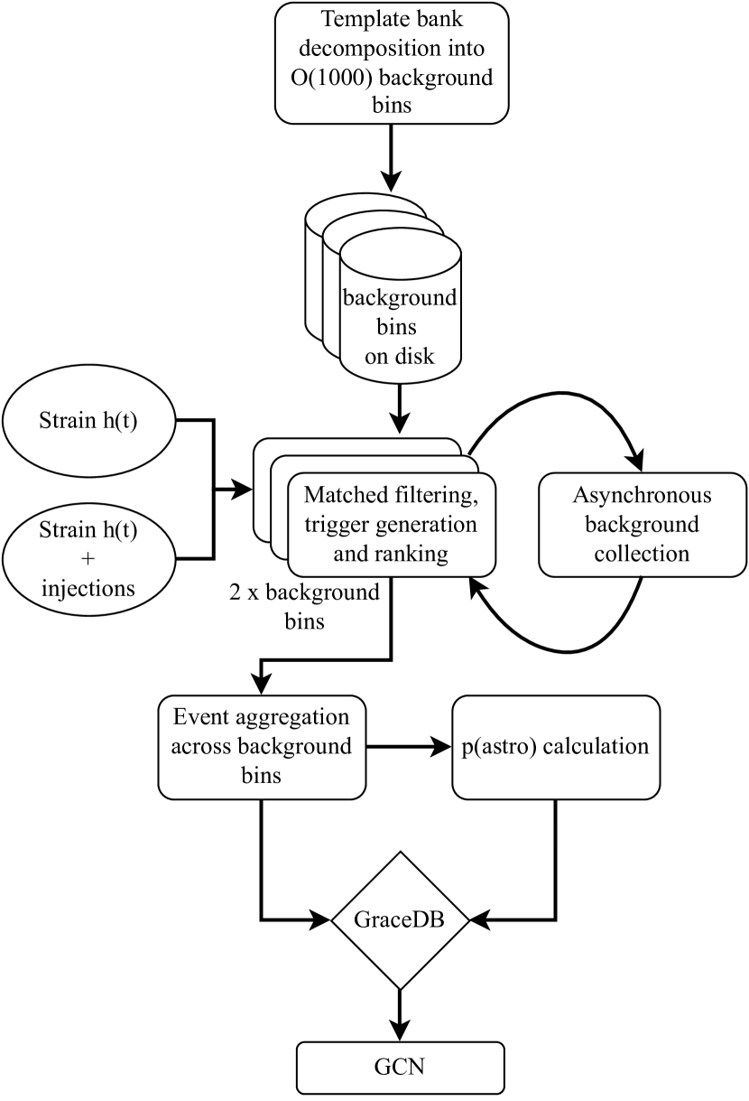
The low-latency GstLAL inspiral workflow consists of two broad stages: a set up stage where pre-computed data products are generated and stored on disk and a persistent analysis stage where strain data is filtered in near real time and candidate events are identified. We will give a brief description of the current workflow and configuration choices to be used in operating the GstLAL analysis during O4. A diagram of the low-latency workflow is shown in Fig. 1. For a more detailed description of the GstLAL analysis methods as of the end of O1 and O2 see [Messick:2016aqy] and [Sachdev:2019vvd], respectively. The GstLAL software package is described in [Cannon:2020qnf].
Before the GstLAL analysis is launched, the template bank is first split into two halves in a process referred to as “checkerboarding”. Each checkerboarded bank is constructed by taking alternating neighboring templates from the full bank. The checkerboarded banks are redundant as they cover the same parameter space while having unique individual templates. The effectualness of the checkerboarded banks is validated in [Sakon:2022ibh]. With this configuration the overall analysis can be split across two independent computing sites which improves the robustness of the analysis to upstream failures. According to the Low-Latency Online Inspiral Detection (LLOID) method, the checkerboarded template banks must then be split into independent bins of waveforms, hereafter referred to as background bins, as shown in Fig. 1. A full derivation and motivation of the LLOID method, including the singular value decomposition (SVD) and template time-slicing, is given by [Cannon:2011vi]. We first sort the template bank by the orthogonal Post-Newtonian (PN) phase terms and . These are linear combinations of the PN coefficients, , , and , defined as follows [Morisaki:2020oqk]:
| (1) |
Using these parameters to sort, we split the template bank into sub-banks each with templates. Each background bin is then constructed by grouping sub-banks together. When computing the decomposition, we require a match between the re-constructed template waveforms and the initial physical waveforms. This value is chosen by balancing the need for computational efficiency with the need for accurately reconstructed waveforms. For the checkerboarded O4 template bank in [Sakon:2022ibh], this produces background bins.
As part of the background bank construction during the set up stage of the analysis, the SVD waveforms are also whitened. For the initial whitening before filtering has begun, we use a reference power spectral density (PSD). As the analysis stage proceeds we will re-whiten the SVD waveforms on a weekly timescale using recent PSDs in order to account for any long term changes to the detector characteristic noise. As the analysis runs, the PSD is continuously tracked using a fast Fourier transform (FFT) length of . Such a short length of FFT in the whitening stage of the pipeline reduces latency at the cost of a less accurate PSD measurement which could potentially bring a loss in sensitivity while filtering.
The low-latency analysis ingests strain data, as well as data quality and interferometer state information from frame files. Each frame includes of data. The frames are distributed from the detectors via Apache Kafka, an open source event streaming platform. After streaming from the detector sites, frames are stored in shared memory partitions, where they are accessed by the GstLAL analysis. The frames are then processed in buffers at a time by each filtering job in the GstLAL pipeline as shown in Fig. 1. In O4, the GstLAL pipeline will also ingest a parallel stream of strain data including simulated compact binary coalescence (CBC) signals injected into the data. These injections will be based on the inferred astrophysical distribution of sources based on the Gravitational Wave Transient Catalog (GWTC-3) [KAGRA:2021duu].
It is known that the LIGO and Virgo data are not “well-behaved” and include non-transient and non-Gaussian noise components known as glitches. These glitches can be mistaken for astrophysical signals, especially high mass BBH templates which are short in duration within the LIGO-Virgo frequency band. To mitigate the negative effects of non-Gaussian data, the GstLAL pipeline gates particularly glitchy whitened strain data using a threshold on the amplitude of the data in units of standard deviations. In gating the strain data, we must be careful to balance the desire to reduce false positives (i.e. mistaking a glitch for an astrophysical signal) with the desire to avoid false negatives (i.e. mistaking an astrophysical signal for a glitch). Since we know that signals from heavy mass CBC systems (for example, IMBH binaries) tend to resemble glitches, we want to be conservative with gating data while filtering templates in this region of the parameter space. For this reason, we choose a mass-dependent gate threshold calculated for each background bin as follows. We first compute a gate ratio defined as:
| (2) |
where we choose the minimum and maximum gate thresholds, and as and , respectively. The chirp mass, , is defined by the following combination of the binary component masses:
| (3) |
The minimum and maximum are taken to be and . Then, the gate threshold is calculated for each background bin as:
| (4) |
Here, is the difference between the maximum in the given background bin and the . This produces gate thresholds ranging from for the smallest mass bins to for the largest mass bins.
In the O4 configuration, we choose a filtering stride of , meaning that the matched filter output is computed in stretches of at a time. The small stride is chosen to reduce latency in the filtering stage. Triggers are defined by peaks in the SNR time-series output by the matched filtering which pass a threshold of . The GstLAL analysis has allowed for single detector candidates since O2 and will continue to do so in O4. However, when calculating the likelihood ratio of single detector candidates we apply a penalty to down rank their significance. This is a tunable parameter and the value to be used in O4 will be discussed in more detail in Sec. III.2. Coincident candidates include triggers from the same template in at least two detectors. We require that the end times of coincident triggers be within of each other after accounting for the light travel time between detectors. Together, the coincidence threshold and the requirement that triggers across detectors ring up the same template provide a strong signal consistency test for candidate events.
The GstLAL pipeline uses the likelihood ratio as a ranking statistic to assign significance to gravitational wave candidates [Cannon:2012zt, Cannon:2015gha]. Recent improvements to the likelihood ratio computation towards O4 are given in [Tsukada:2023edh]. These include an upgraded analytic SNR- signal model and a method for removing signal contamination from the background which is also described in [Joshi:2023ltf]. The background noise in each detector is estimated by collecting ranking statistic data from single-detector triggers observed in coincident time. We exclude triggers from times when only one detector is operating since these triggers may be astrophysical signals. These background estimations are cumulative and “snapshotted” to disk every hours. The filtering jobs which process injection strain data do not collect their own background estimations. This is because the high rate of injected signals in the data would contaminate the background and corrupt the statistics used for the FAR estimation. Instead, these injection filtering jobs use a copy of the background statistics collected by the corresponding non-injection filtering job which processes the same background bin.
While the pipeline is designed to run persistently, there is need to take the analysis down periodically. We remove each of our analyses for a short period of time on a weekly timescale with a staggered schedule so that at least one of the checkerboarded analyses is always observing. When an analysis is re-launched after this weekly downtime, we compress the background ranking statistic data by removing any values in the horizon distance history that differ fractionally from their neighbors by less than . This compression reduces the file size and memory use of the pipeline, which would otherwise grow without bounds over the duration of the observing period.
For FAR estimation, the ranking statistic data is marginalized by adding counts from the SNR- background distributions collected in each background bin. The histograms are marginalized over in a continuous loop, taking several hours to complete each iteration. The marginalization is cumulative in time so that as the run proceeds, we collect more and more background counts. To account for the two redundant checkerboarded analyses, we apply a FAR trials factor of to each trigger.
Gravitational wave events passing a FAR threshold of one per hour will be uploaded to the Gravitational wave Candidate Event Database (GraceDB) [gracedb]. Because the GstLAL pipeline filters the strain data in independent background bins, it is not only possible but highly probable that there will be multiple triggers associated with each physical gravitational wave candidate. The number of triggers per candidate could range from a few for quieter signals to several tens for louder signals. In order to reduce API calls to GraceDB we aggregate these triggers in time across background bins by the maximum SNR and only upload the current best candidate. In this aggregation stage, triggers from different background bins are grouped into candidates using a coincidence window defined by rounding down to the nearest half second and rounding up to the nearest half second. Here, is the end time of the trigger and seconds. The first trigger received by the aggregator for a given candidate is uploaded to GraceDB immediately. Any subsequent triggers for the same candidate which are found with higher SNR are uploaded with a second geometric wait time. That is, after the first upload, the second upload will not be made until seconds later, the third upload until seconds later, and so on. The aggregation stage of the pipeline is illustrated in Fig. 1.
Finally, the GstLAL pipeline calculates a probability of astrophysical origin, or , for each event uploaded to GraceDB. The is a measure of the event’s significance, and as we also compute the probability that the event originates from each CBC source class (BNS, NSBH, or BBH) it gives an indication of the likelihood that an event will have an electromagnetic counterpart. Therefore, the is an important quantity to help astronomers determine when to follow up gravitational wave candidates. More information about the GstLAL pipeline’s computation of can be found in [Ray:2023nhx].
II.2 GW Low-latency Test Suite
The gw-lts software is designed to provide consistency checks and real-time feedback on the reliability of science outputs of gravitational wave search pipelines. By using simulated signals injected in the strain data, we can compare the pipeline performance to what is expected.
The Test Suite requires a source of truth for the signals that are present in the data. For this, we rely on an injection set on disk which defines all of the injections, including all intrinsic and extrinsic parameters, and the Global Positioning System (GPS) times at which they appear in the strain data. Using a live estimate of the PSD and the injected signal’s sky location we can compute the expected SNR. For information about recovered events, GraceDB is taken as the source of truth. The igwn-alert software package is a messaging system built on Apache Kafka which sends notifications of GraceDB state changes to subscribed users. The Test Suite subscribes to notifications from igwn-alert which are sent for any new or updated event on GraceDB. The injections are then matched with recovered alerts in low-latency by finding coincidences within a small which we take to be seconds. This time window was chosen to be very small compared to a typical injection rate to avoid erroneous coincidences.
Once an injected signal is matched with a recovered event, the information is passed to an arbitrary number of independent jobs via Apache Kafka. The jobs compute metrics associated with the injection recovery such as the , accuracy of source classification and sky localization, and accuracy of point estimates of the source intrinsic parameters. The gw-lts capabilities are described in further detail in Section III.
All of the metrics computed by the gw-lts are stored with InfluxDB, which is an open source platform for storing and querying time series data. We use the data visualization tool Grafana to display the data in real time in online dashboards. With this infrastructure, we are able to track changes in the performance of the analysis on the timescale of seconds. Additionally, from the Influx database we are able to keep an archival record of the performance metrics.
III Mock data challenge results
To demonstrate the performance of the GstLAL analysis and our readiness for O4, we participated in a MDC consisting of a forty day stretch of HLV O3 strain data taken from 5 Jan. 2020 15:59:42 to 14 Feb. 2020 15:59:42 UTC and replayed so as to be analyzed in a low-latency configuration. The MDC also provided a set of identical strain channels with injected BNS, NSBH, and BBH signals. Details of the injection distributions used in the MDC can be found in [mdc_analytics]. Injected signals were placed in the strain data at a rate of one per seconds, leading to a total of total injections throughout the MDC duration.
In this section we seek to quantify the performance of the GstLAL pipeline in its latest configuration. We will first show the recovery of known gravitational wave events in the MDC data, as well as highlight any potential retraction level events. We will then detail the results of the MDC injection campaign. Finally we present the stability and performance of the pipeline in terms of its uptime and latency.
III.1 Gravitational wave events
There are gravitational wave events in the duration of the MDC replay data which were previously published as significant candidates in GWTC-3 [LIGOScientific:2021djp]. These are described throughout the remainder of this section and summarized in Table 1, comparing the GstLAL pipeline’s recovery of the signal in O3 to that in the MDC. We recover all of the candidates at the per hour FAR threshold for uploading to GraceDB. Of these, three were found with high significance by GstLAL in the O3 online analysis. Two were found with marginal or sub-threshold significance online but with high significance offline. Four candidates were only found by GstLAL in the offline analysis. The recovery of all previously published candidates shows that the pipeline is performing with at least the same capability as in O3.
| O3 Online | MDC | |||||||
| Name | Inst | SNR | FAR | Inst | SNR | FAR | ||
| () | () | |||||||
| GW | \IfEqCaseGW200112GW200112L1GW200115H1L1GW200128–GW200129H1L1V1GW200202–GW200208q–GW200208am–GW200209–GW200210–[] | \IfEqCaseGW200112GW200112GW200115GW200128–GW200129GW200202–GW200208q–GW200208am–GW200209–GW200210–[] | \IfEqCaseGW200112GW200112GW200115GW200128GW200129GW200202GW200208q–GW200208am–GW200209–GW200210–[] | \IfEqCaseGW200112GW200112GW200115GW200128–GW200129GW200202–GW200208q–GW200208am–GW200209–GW200210–[] | \IfEqCaseGW200112GW200112L1GW200115H1L1GW200128H1L1GW200129H1L1V1GW200202H1L1GW200208qH1L1GW200208amH1L1GW200209H1L1GW200210H1L1[] | \IfEqCaseGW200112GW200112GW200115GW200128GW200129GW200202GW200208qGW200208amGW200209GW200210[] | \IfEqCaseGW200112GW200112GW200115GW200128GW200129GW200202GW200208qGW200208amGW200209GW200210[] | \IfEqCaseGW200112GW200112GW200115GW200128GW200129GW200202GW200208qGW200208amGW200209GW2002100.27[] |
| GW | \IfEqCaseGW200115GW200112L1GW200115H1L1GW200128–GW200129H1L1V1GW200202–GW200208q–GW200208am–GW200209–GW200210–[] | \IfEqCaseGW200115GW200112GW200115GW200128–GW200129GW200202–GW200208q–GW200208am–GW200209–GW200210–[] | \IfEqCaseGW200115GW200112GW200115GW200128GW200129GW200202GW200208q–GW200208am–GW200209–GW200210–[] | \IfEqCaseGW200115GW200112GW200115GW200128–GW200129GW200202–GW200208q–GW200208am–GW200209–GW200210–[] | \IfEqCaseGW200115GW200112L1GW200115H1L1GW200128H1L1GW200129H1L1V1GW200202H1L1GW200208qH1L1GW200208amH1L1GW200209H1L1GW200210H1L1[] | \IfEqCaseGW200115GW200112GW200115GW200128GW200129GW200202GW200208qGW200208amGW200209GW200210[] | \IfEqCaseGW200115GW200112GW200115GW200128GW200129GW200202GW200208qGW200208amGW200209GW200210[] | \IfEqCaseGW200115GW200112GW200115GW200128GW200129GW200202GW200208qGW200208amGW200209GW2002100.27[] |
| GW | \IfEqCaseGW200128GW200112L1GW200115H1L1GW200128–GW200129H1L1V1GW200202–GW200208q–GW200208am–GW200209–GW200210–[] | \IfEqCaseGW200128GW200112GW200115GW200128–GW200129GW200202–GW200208q–GW200208am–GW200209–GW200210–[] | \IfEqCaseGW200128GW200112GW200115GW200128GW200129GW200202GW200208q–GW200208am–GW200209–GW200210–[] | \IfEqCaseGW200128GW200112GW200115GW200128–GW200129GW200202–GW200208q–GW200208am–GW200209–GW200210–[] | \IfEqCaseGW200128GW200112L1GW200115H1L1GW200128H1L1GW200129H1L1V1GW200202H1L1GW200208qH1L1GW200208amH1L1GW200209H1L1GW200210H1L1[] | \IfEqCaseGW200128GW200112GW200115GW200128GW200129GW200202GW200208qGW200208amGW200209GW200210[] | \IfEqCaseGW200128GW200112GW200115GW200128GW200129GW200202GW200208qGW200208amGW200209GW200210[] | \IfEqCaseGW200128GW200112GW200115GW200128GW200129GW200202GW200208qGW200208amGW200209GW2002100.27[] |
| GW | \IfEqCaseGW200129GW200112L1GW200115H1L1GW200128–GW200129H1L1V1GW200202–GW200208q–GW200208am–GW200209–GW200210–[] | \IfEqCaseGW200129GW200112GW200115GW200128–GW200129GW200202–GW200208q–GW200208am–GW200209–GW200210–[] | \IfEqCaseGW200129GW200112GW200115GW200128GW200129GW200202GW200208q–GW200208am–GW200209–GW200210–[] | \IfEqCaseGW200129GW200112GW200115GW200128–GW200129GW200202–GW200208q–GW200208am–GW200209–GW200210–[] | \IfEqCaseGW200129GW200112L1GW200115H1L1GW200128H1L1GW200129H1L1V1GW200202H1L1GW200208qH1L1GW200208amH1L1GW200209H1L1GW200210H1L1[] | \IfEqCaseGW200129GW200112GW200115GW200128GW200129GW200202GW200208qGW200208amGW200209GW200210[] | \IfEqCaseGW200129GW200112GW200115GW200128GW200129GW200202GW200208qGW200208amGW200209GW200210[] | \IfEqCaseGW200129GW200112GW200115GW200128GW200129GW200202GW200208qGW200208amGW200209GW2002100.27[] |
| GW | \IfEqCaseGW200202GW200112L1GW200115H1L1GW200128–GW200129H1L1V1GW200202–GW200208q–GW200208am–GW200209–GW200210–[] | \IfEqCaseGW200202GW200112GW200115GW200128–GW200129GW200202–GW200208q–GW200208am–GW200209–GW200210–[] | \IfEqCaseGW200202GW200112GW200115GW200128GW200129GW200202GW200208q–GW200208am–GW200209–GW200210–[] | \IfEqCaseGW200202GW200112GW200115GW200128–GW200129GW200202–GW200208q–GW200208am–GW200209–GW200210–[] | \IfEqCaseGW200202GW200112L1GW200115H1L1GW200128H1L1GW200129H1L1V1GW200202H1L1GW200208qH1L1GW200208amH1L1GW200209H1L1GW200210H1L1[] | \IfEqCaseGW200202GW200112GW200115GW200128GW200129GW200202GW200208qGW200208amGW200209GW200210[] | \IfEqCaseGW200202GW200112GW200115GW200128GW200129GW200202GW200208qGW200208amGW200209GW200210[] | \IfEqCaseGW200202GW200112GW200115GW200128GW200129GW200202GW200208qGW200208amGW200209GW2002100.27[] |
| GW | \IfEqCaseGW200208qGW200112L1GW200115H1L1GW200128–GW200129H1L1V1GW200202–GW200208q–GW200208am–GW200209–GW200210–[] | \IfEqCaseGW200208qGW200112GW200115GW200128–GW200129GW200202–GW200208q–GW200208am–GW200209–GW200210–[] | \IfEqCaseGW200208qGW200112GW200115GW200128GW200129GW200202GW200208q–GW200208am–GW200209–GW200210–[] | \IfEqCaseGW200208qGW200112GW200115GW200128–GW200129GW200202–GW200208q–GW200208am–GW200209–GW200210–[] | \IfEqCaseGW200208qGW200112L1GW200115H1L1GW200128H1L1GW200129H1L1V1GW200202H1L1GW200208qH1L1GW200208amH1L1GW200209H1L1GW200210H1L1[] | \IfEqCaseGW200208qGW200112GW200115GW200128GW200129GW200202GW200208qGW200208amGW200209GW200210[] | \IfEqCaseGW200208qGW200112GW200115GW200128GW200129GW200202GW200208qGW200208amGW200209GW200210[] | \IfEqCaseGW200208qGW200112GW200115GW200128GW200129GW200202GW200208qGW200208amGW200209GW2002100.27[] |
| GW | \IfEqCaseGW200208amGW200112L1GW200115H1L1GW200128–GW200129H1L1V1GW200202–GW200208q–GW200208am–GW200209–GW200210–[] | \IfEqCaseGW200208amGW200112GW200115GW200128–GW200129GW200202–GW200208q–GW200208am–GW200209–GW200210–[] | \IfEqCaseGW200208amGW200112GW200115GW200128GW200129GW200202GW200208q–GW200208am–GW200209–GW200210–[] | \IfEqCaseGW200208amGW200112GW200115GW200128–GW200129GW200202–GW200208q–GW200208am–GW200209–GW200210–[] | \IfEqCaseGW200208amGW200112L1GW200115H1L1GW200128H1L1GW200129H1L1V1GW200202H1L1GW200208qH1L1GW200208amH1L1GW200209H1L1GW200210H1L1[] | \IfEqCaseGW200208amGW200112GW200115GW200128GW200129GW200202GW200208qGW200208amGW200209GW200210[] | \IfEqCaseGW200208amGW200112GW200115GW200128GW200129GW200202GW200208qGW200208amGW200209GW200210[] | \IfEqCaseGW200208amGW200112GW200115GW200128GW200129GW200202GW200208qGW200208amGW200209GW2002100.27[] |
| GW | \IfEqCaseGW200209GW200112L1GW200115H1L1GW200128–GW200129H1L1V1GW200202–GW200208q–GW200208am–GW200209–GW200210–[] | \IfEqCaseGW200209GW200112GW200115GW200128–GW200129GW200202–GW200208q–GW200208am–GW200209–GW200210–[] | \IfEqCaseGW200209GW200112GW200115GW200128GW200129GW200202GW200208q–GW200208am–GW200209–GW200210–[] | \IfEqCaseGW200209GW200112GW200115GW200128–GW200129GW200202–GW200208q–GW200208am–GW200209–GW200210–[] | \IfEqCaseGW200209GW200112L1GW200115H1L1GW200128H1L1GW200129H1L1V1GW200202H1L1GW200208qH1L1GW200208amH1L1GW200209H1L1GW200210H1L1[] | \IfEqCaseGW200209GW200112GW200115GW200128GW200129GW200202GW200208qGW200208amGW200209GW200210[] | \IfEqCaseGW200209GW200112GW200115GW200128GW200129GW200202GW200208qGW200208amGW200209GW200210[] | \IfEqCaseGW200209GW200112GW200115GW200128GW200129GW200202GW200208qGW200208amGW200209GW2002100.27[] |
| GW | \IfEqCaseGW200210GW200112L1GW200115H1L1GW200128–GW200129H1L1V1GW200202–GW200208q–GW200208am–GW200209–GW200210–[] | \IfEqCaseGW200210GW200112GW200115GW200128–GW200129GW200202–GW200208q–GW200208am–GW200209–GW200210–[] | \IfEqCaseGW200210GW200112GW200115GW200128GW200129GW200202GW200208q–GW200208am–GW200209–GW200210–[] | \IfEqCaseGW200210GW200112GW200115GW200128–GW200129GW200202–GW200208q–GW200208am–GW200209–GW200210–[] | \IfEqCaseGW200210GW200112L1GW200115H1L1GW200128H1L1GW200129H1L1V1GW200202H1L1GW200208qH1L1GW200208amH1L1GW200209H1L1GW200210H1L1[] | \IfEqCaseGW200210GW200112GW200115GW200128GW200129GW200202GW200208qGW200208amGW200209GW200210[] | \IfEqCaseGW200210GW200112GW200115GW200128GW200129GW200202GW200208qGW200208amGW200209GW200210[] | \IfEqCaseGW200210GW200112GW200115GW200128GW200129GW200202GW200208qGW200208amGW200209GW2002100.27[] |
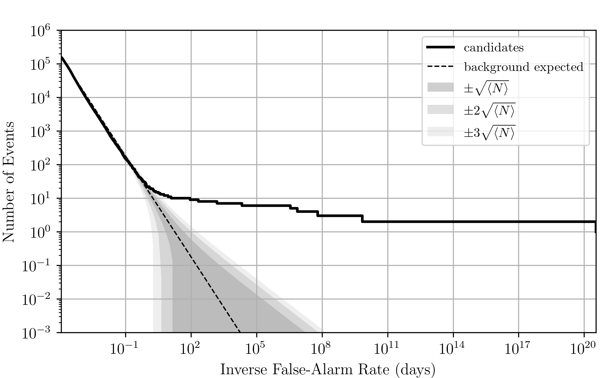
Fig. 2 shows the count of observed candidates versus inverse false alarm rate (IFAR). The expected background counts are calculated using an estimated livetime which is equal to the wall clock time from the first to the last candidate. Additionally, we apply a trials factor of to the FARs since we only include candidates from one of the checkerboarded analyses. Fig. 2 shows the known gravitational wave events recovered in the MDC. The candidate IFAR statistics agree with the expected counts from noise at lower IFAR and diverge due to the presence of signals at higher IFAR.
This event was a BBH candidate observed in LIGO Livingston data as a single detector candidate with chirp mass \IfEqCaseGW200112GW200112GW200115GW200128–GW200129GW200202–GW200208q–GW200208am–GW200209–GW200210–[] in O3 and \IfEqCaseGW200112GW200112GW200115GW200128GW200129GW200202GW200208qGW200208amGW200209GW200210[] in the MDC. In the MDC, we recover the event with a comparable SNR as that observed in O3, however in the MDC the FAR is significantly lower.
was the first confident NSBH detection found in O3. The event was found as a coincident trigger in LIGO Hanford and LIGO Livingston data. The SNR recovery, FAR estimation, and chirp mass estimation are all equivalent in the MDC to what was observed in O3.
was a BBH and the loudest gravitational wave signal in the duration of the MDC with O3 SNR . The event was recovered well below the public alert threshold in both O3 and the MDC.
and are both BBH candidates found by GstLAL in the O3 online analysis with low significance. Both candidates were found with FAR above the O3 public alert threshold of per year, where a trials factor corresponding to the number of operating pipelines has been applied. Later, during the offline analysis they were recovered as significant candidates and included in GWTC-3 [LIGOScientific:2021djp]. In the MDC we recover both candidates with significantly lower FARs, both well below the public alert threshold. Therefore, if similar events occur during O4, we can expect to recover them as significant public alerts.
was not recovered by GstLAL in the O3 online analysis, however it was found in the offline analysis by GstLAL as a marginally significant candidate [LIGOScientific:2021djp]. As recovered in the MDC, this event is a BBH candidate with chirp mass \IfEqCaseGW200208qGW200112GW200115GW200128GW200129GW200202GW200208qGW200208amGW200209GW200210[] and a much lower FAR than what was found in either the O3 online or offline analyses.
was only recovered by GstLAL as a sub-threshold candidate in the O3 offline analysis, and its inclusion as a significant candidate in GWTC-3 was due to its recovery by other CBC pipelines [LIGOScientific:2021djp]. The GstLAL pipeline did not recover this event in O3 online. In the MDC the event was recovered with low significance at SNR and FAR per year.
and were not recovered by GstLAL in the O3 online analysis, however they were found in the offline analysis by GstLAL with high significance and marginal significance, respectively. In the MDC, was recovered as a high significance candidate with FAR per year. This event is a BBH candidate with chirp mass found in LIGO Hanford and LIGO Livingston data. was found as a sub-threshold candidate in the MDC with FAR per year. If astrophysical, the event would be an NSBH candidate with chirp mass .
The improved performance of the GstLAL pipeline in the MDC as compared to the O3 online analysis can be attributed to a number of incremental improvements made to the likelihood ratio ranking statistic and background estimation. [Tsukada:2023edh] describes an improved signal model and [Joshi:2023ltf] introduces a new method for a time-dependent background wherein contamination is reduced by removing signals counts from the background histograms. Each of these changes have introduced a small improvement to the which, when combined, leads to a noticeable increase in sensitivity and corresponding number of detected events.
III.2 Retractions
In O3, there were 23 public gravitational wave candidates which were subsequently determined to be terrestrial in origin and thus retracted. Of these, GstLAL contributed to 15. In O4, we hope to significantly reduce the number of retractions produced by the GstLAL pipeline. Four of the 23 retractions took place during the stretch of data covered by the MDC. These are: S200106au, S200106av, S200108v, and S200116ah [GCN26641, GCN26665, GCN26785].
GstLAL did not upload triggers for S200106au and S200106av during O3. In the MDC, these events would have occurred at a time before the pipeline had collected sufficient background to begin ranking candidates, and thus we did not upload triggers for these events. The retractions S200108v and S200116ah were GstLAL-only candidates in O3, both being found as L single detector candidates. Again, the time corresponding to S200108v would have been early enough in the MDC cycle that the pipeline was not ranking or uploading triggers yet, so we cannot make any comparison to our performance in O3 for this retraction. Finally, we did not produce any trigger below the per hour FAR threshold for uploading to GraceDB corresponding to S200116ah in the MDC, despite the analysis being fully burned in and operating in a stable state. This indicates an improvement in our rate of retractions for O4, however there is not enough data within the MDC to make a strong statement.
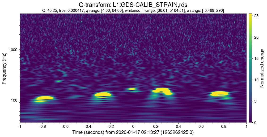
In addition to the retracted candidates uploaded by GstLAL in O3, for the purpose of the MDC we define a “retraction level candidate” as any gravitational wave candidate uploaded with a FAR less than one per year which is not in the list of previously published candidates discussed earlier in this section. Over the duration of the MDC, we find one such retraction level candidate. This was a single-detector candidate found in L with an SNR of . The recovered FAR was low enough to be counted as a significant candidate with FAR . The L data around the event time shows the clear presence of scattering glitches, as shown in Fig. 3. Further evidence of terrestrial origin for this candidate is that no coincident triggers were recovered in H or V despite both of these detectors operating normally at the time. Candidates recovered in only a single detector are more susceptible to uncertainty since they lack the strong signal consistency test of coincidence in multiple detectors. For this reason, there has been a penalty applied to the ranking statistic of single detector candidates which down weights their significance. In the O3 offline analysis and in the MDC we used a singles penalty of in log likelihood ratio, however in order to reduce the number of similar retraction level events in O4, we plan to increase the singles penalty to . With this penalty applied, the retraction event in the MDC would be down weighted and expected to be recovered with a FAR greater than two per year.
III.3 Recovered injections
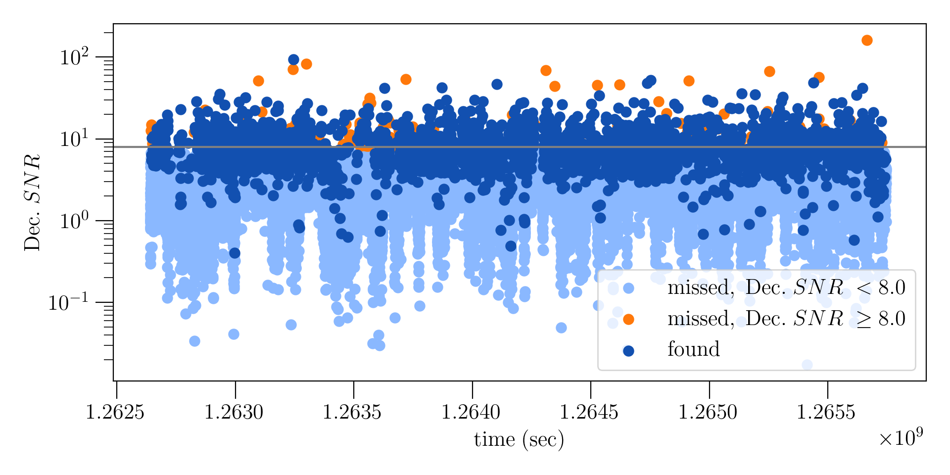
There were simulated signals injected into the five week duration of the MDC strain data. Of these, many had component masses and spins outside the region of parameter space covered by our template bank. In addition to the injection parameters, the expected recovery of each injection is dependent on the set of interferometers producing science quality data at the time of the injection. During times when no interferometers are operating we of course do not expect to recover any injections. We define the decisive SNR as the SNR in the second most sensitive interferometer during times when multiple interferometers were observing, and the only available SNR otherwise. The decisive SNR is a more informative measure of the loudness of an injection than the network SNR since it wraps in information about the set of operating interferometers. While all injections have network SNR , we find that many injections have decisive SNR .
Fig. 4 shows the time-series of decisive SNR for all injections throughout the MDC. For the purpose of this paper, we focus on injections whose parameters fall inside our bank. That is, injections with component masses between and , with total masses, and mass ratios, . For objects with mass the template bank restricts spins perpendicular to the orbital plane to be , and for objects with mass allows spins up to . We use the effective precession spin, , defined in [Schmidt:2014iyl] as:
| (5) |
to quantify the in-plane spin of injections. Here, , , and . And is the mass ratio, taking . Since the template bank does not include any in-plane spins, we focus on injections with . However, we find that all injections with one component mass have spins outside the range of the bank, therefore we relax the spin conditions on these components. The mass and spin restrictions that we use are summarized in Table 2. Finally, to account for the fact that not all interferometers were providing science quality data at all times, we highlight injections with an estimated decisive SNR . These cuts leave a total of injections during the five week MDC. Of these, there are BBH, BNS, and NSBH injections.
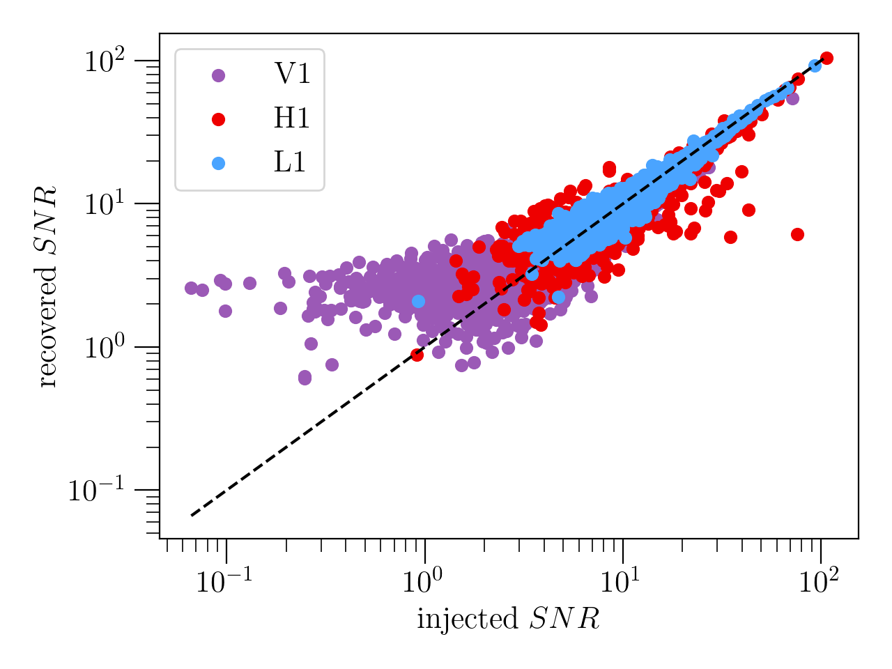
The injected SNRs are not known in advance of the MDC, but we estimate them using gw-lts. We calculate the injected strain time series using the injection end time, sky position, and other source intrinsic parameters assuming an IMRPhenomPv2_NRTidalv2 waveform [Dietrich:2019kaq]. We use a running estimate of the detector PSDs and estimate the SNR with a lower (upper) frequency cut off of () Hz. Fig. 5 shows the recovered and estimated injected SNR for each detector. If the template bank did not have a sufficient minimal match, we may expect to see systematically lower recovered SNRs than the expected values. However, we find that the recovered SNR generally aligns with the expected SNR.
| – | – | – | ||||
| – | – | – | ||||
An injection is considered “found” if it is recovered by the pipeline with a FAR passing some pre-determined threshold, and “missed” otherwise. We will quote most results in the following sections with respect to a per day FAR threshold. At the time of writing, this is the threshold expected to be used in O4 for sending public alerts [user_guide]. However, the FARs of CBC signals will be subject to a trials factor corresponding to the number of operating pipelines, so the effective alert threshold will be lower. We define the injection recovery efficiency as,
| (6) |
At the per day FAR threshold the efficiency was for all injections in the template bank. The recovered injection efficiencies for each source class are shown in Table 3 at four typical FAR thresholds. As is expected, the efficiencies are better at more conservative FAR thresholds. The analysis has the highest efficiency for injections consistent with BNS sources, and the lowest efficiency for NSBH sources.
We would expect the pipeline to recover all injections above some decisive SNR or network SNR threshold. However, Fig. 4 shows that there are several very high SNR missed injections throughout the duration of the MDC. We find that most of the missed injections with decisive SNR are high mass BBH injections and a few are high mass ratio NSBH injections. This results in a decrease of the BBH recovery efficiency as the injections increase in SNR, which is contradictory to our expectations. These injections are missed due to falling outside of the SNR- signal region used in the likelihood ratio calculation. The signal region is an analytic model which depends on the allowed mismatch111The “mismatch” can also mean the fractional loss in SNR due to differences between the template parameters and the true waveform. However, here we refer to the mismatch as defined in [Tsukada:2023edh] which is an unnormalized quantity, therefore retaining a dependence on the SNR. between recovered SNR time-series and the template waveform as part of the autocorrelation test. If the allowed mismatch range is too strict, it will result in a narrow signal model which can exclude real signals. This effect is exaggerated at high SNR where we expect larger mismatches due to the discreteness of the template bank as well as waveform systematics. In the MDC, we used a mismatch range of . The optimal mismatch range in the signal model is an open area of study. See [Tsukada:2023edh] for a more detailed discussion.
| FAR | BNS | NSBH | BBH | ALL |
|---|---|---|---|---|
| \IfEqCaseONEPERHOURONEPERHOURTWOPERDAYONEPERMONTHTWOPERYEAR[] | \IfEqCaseONEPERHOURONEPERHOURTWOPERDAYONEPERMONTHTWOPERYEAR[] | \IfEqCaseONEPERHOURONEPERHOURTWOPERDAYONEPERMONTHTWOPERYEAR[] | \IfEqCaseONEPERHOURONEPERHOURTWOPERDAYONEPERMONTHTWOPERYEAR[] | |
| \IfEqCaseTWOPERDAYONEPERHOURTWOPERDAYONEPERMONTHTWOPERYEAR[] | \IfEqCaseTWOPERDAYONEPERHOURTWOPERDAYONEPERMONTHTWOPERYEAR[] | \IfEqCaseTWOPERDAYONEPERHOURTWOPERDAYONEPERMONTHTWOPERYEAR[] | \IfEqCaseTWOPERDAYONEPERHOURTWOPERDAYONEPERMONTHTWOPERYEAR[] | |
| \IfEqCaseONEPERMONTHONEPERHOURTWOPERDAYONEPERMONTHTWOPERYEAR[] | \IfEqCaseONEPERMONTHONEPERHOURTWOPERDAYONEPERMONTHTWOPERYEAR[] | \IfEqCaseONEPERMONTHONEPERHOURTWOPERDAYONEPERMONTHTWOPERYEAR[] | \IfEqCaseONEPERMONTHONEPERHOURTWOPERDAYONEPERMONTHTWOPERYEAR[] | |
| \IfEqCaseTWOPERYEARONEPERHOURTWOPERDAYONEPERMONTHTWOPERYEAR[] | \IfEqCaseTWOPERYEARONEPERHOURTWOPERDAYONEPERMONTHTWOPERYEAR[] | \IfEqCaseTWOPERYEARONEPERHOURTWOPERDAYONEPERMONTHTWOPERYEAR[] | \IfEqCaseTWOPERYEARONEPERHOURTWOPERDAYONEPERMONTHTWOPERYEAR[] |
III.3.1 Injection parameter recovery
In this section we will quantify the accuracy of point estimates of the source intrinsic parameters made by the GstLAL pipeline. These estimates simply come from the template parameters of the trigger which rang up the maximum SNR across background bins. An understanding of the parameter accuracy obtained by search pipelines can be useful to full parameter estimation efforts. For example, the Bayesian inference library Bilby [Smith:2019ucc, Ashton:2018jfp] relies on the choice of prior probability distributions for intrinsic parameters. When parameters are well determined by the searches, Bilby can use narrow distributions around those values, otherwise more broad prior distributions must be used. We present parameter accuracy results for the chirp mass , effective inspiral spin , mass ratio , and the coalescence end time, . The is a mass-weighted combination of the component spins parallel to the orbital angular momentum , defined as:
| (7) |
where we take to be in the -direction. Both the injected and recovered masses quoted in this paper are in the detector frame. The error on a recovered parameter, is defined as:
| (8) |
for all parameters except for the end time, where we simply take the error as the difference between the recovered and injected end times in milliseconds.
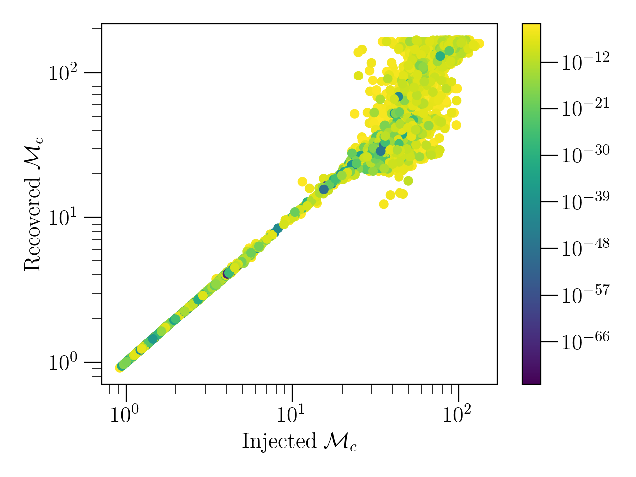
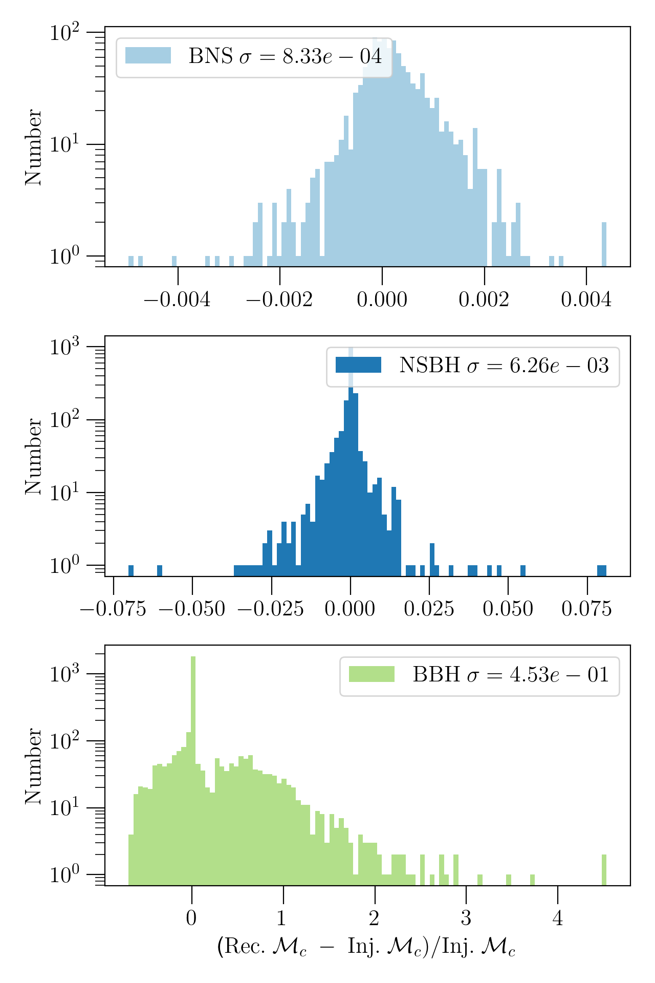
It is well known that the chirp mass, , is one of the best measured parameters in gravitational wave detections, however the recovered accuracy is highly dependent upon the mass of the system. Injections with small are recovered with very accurate , but above this level, the accuracy starts to fall off, as shown in Fig. 6. For BNS injections, we find a mean error with a standard deviation of . Similarly, the in the NSBH region is recovered very well with mean and standard deviation . The BBH region has a higher error over all, and additionally a much larger spread in the error with mean and standard deviation . Histograms of the recovered error for each source class are shown in Fig. 7.
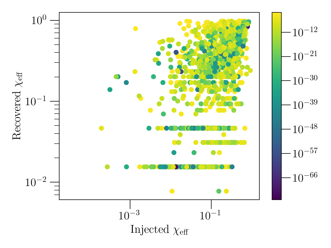
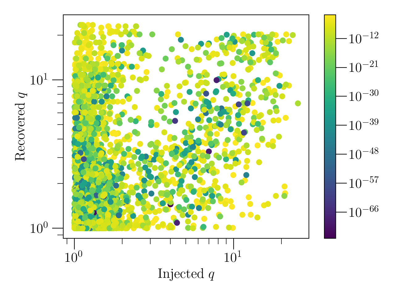
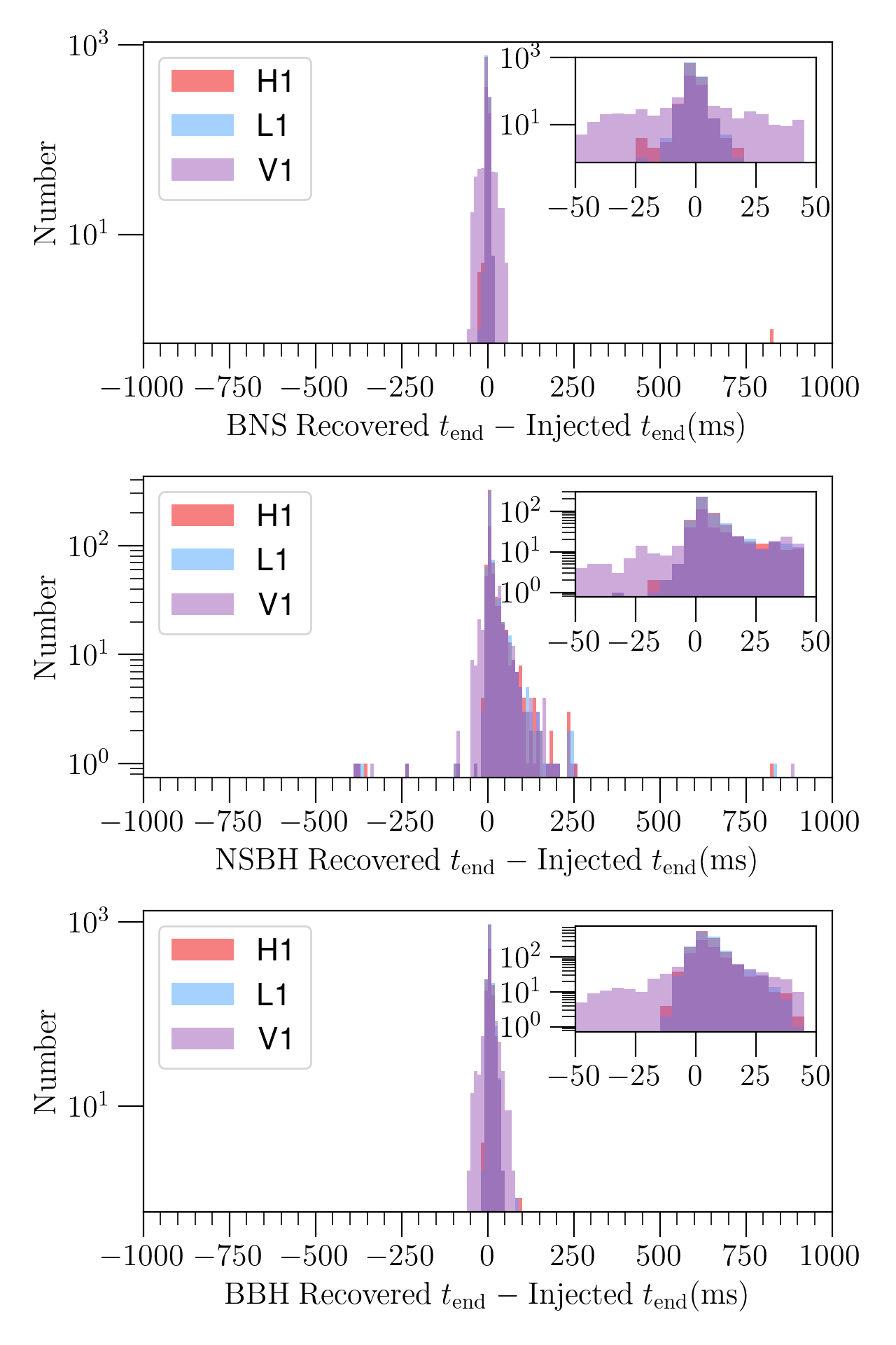
Fig. 8 and Fig. 9 are scatter plots of the injected and recovered and respectively. These plots show that there is very little correlation between the injected and recovered values of these parameters. The mean and standard deviation on the recovered error for these parameters are given in Table LABEL:tab:param-acc.
A histogram of the difference between the injected and recovered injection end times is given in Fig. 10. Table LABEL:tab:param-acc shows the mean difference across all source classes and detectors is \IfEqCaseENDTIMEMASSRATIOMCHIRPSPIN1ZSPIN2ZCHIEFFENDTIME[