Analysis and numerical simulation of a generalized compressible Cahn-Hilliard-Navier-Stokes model with friction effects

Abstract

Motivated by the mathematical modeling of tumor invasion in healthy tissues, we propose a generalized compressible diphasic Navier-Stokes Cahn-Hilliard model that we name G-NSCH. We assume that the two phases of the fluid represent two different populations of cells: cancer cells and healthy tissue. We include in our model possible friction and proliferation effects. The model aims to be as general as possible to study the possible mechanical effects playing a role in invasive growth of a tumor. In the present work, we focus on the analysis and numerical simulation of the G-NSCH model. Our G-NSCH system is derived rigorously and satisfies basic mechanics of fluids and thermodynamics of particles. Under simplifying assumptions, we prove the existence of global weak solutions. We also propose a structure preserving numerical scheme based on the scalar auxiliary variable method to simulate our system and present some numerical simulations validating the properties of the numerical scheme and illustrating the solutions of the G-NSCH model.

2010 Mathematics Subject Classification. 35B40; 35B45; 35G20 ; 35Q35; 35Q92; 65M08
Keywords and phrases. Cahn-Hilliard equation; Navier-Stokes equation; Asymptotic analysis; Mathematical modeling; Numerical simulations; Scalar Auxiliary Variable method.

1 Introduction

We derive, analyze and simulate numerically the generalized compressible Navier-Stokes-Cahn-Hilliard variant (G-NSCH in short)

$$\frac{\partial\rho}{\partial t}+{\rm div}\left(\rho\mathbf{v}\right)=0,$$ (1.1)

$$\frac{\partial(\rho c)}{\partial t}+{\rm div}\left(\rho c\mathbf{v}\right)={\rm div}\left(b(c)\nabla\mu\right)+F_{c},$$ (1.2)

$$\rho\mu=-\gamma\Delta c+\rho\frac{\partial\psi_{0}}{\partial c},$$ (1.3)

$$\frac{\partial(\rho\mathbf{v})}{\partial t}+{\rm div}\left(\rho\mathbf{v}\otimes\mathbf{v}\right)=\begin{multlined}-\left[\nabla p+\gamma{\rm div}\left(\nabla c\otimes\nabla c-\frac{1}{2}\lvert\nabla c\rvert^{2}\mathbf{1}\right)\right]+{\rm div}\left(\nu(c)\left(\nabla\mathbf{v}+\nabla\mathbf{v}^{T}\right)\right)\\ -\frac{2}{3}\nabla\left(\nu(c)\left({\rm div}\left(\mathbf{v}\right)\right)\right)-\kappa(\rho,c)\mathbf{v},\end{multlined}-\left[\nabla p+\gamma{\rm div}\left(\nabla c\otimes\nabla c-\frac{1}{2}\lvert\nabla c\rvert^{2}\mathbf{1}\right)\right]+{\rm div}\left(\nu(c)\left(\nabla\mathbf{v}+\nabla\mathbf{v}^{T}\right)\right)\\ -\frac{2}{3}\nabla\left(\nu(c)\left({\rm div}\left(\mathbf{v}\right)\right)\right)-\kappa(\rho,c)\mathbf{v},$$ (1.6)

stated in $(0,T)\times\Omega$, where $T>0$ is finite time, and $\Omega\subset\mathbb{R}^{d}$ $(d=1,2,3)$ is an open bounded domain with a smooth boundary $\partial\Omega$.

Interested in the modeling of invasive growth of tumors in healthy tissues, we motivate the different terms of the model with this biological application in mind. System (1.1)–(1.6) models the motion of a diphasic fluid composed of two immiscible components,i.e. the cells of the two different types, in a porous matrix and comprises viscosity effects, surface tension, and friction on the rigid fibers constituting the medium. In System (1.1)–(1.6), $\rho$ is the total density of the mixture (i.e. the sum of the two partial densities), $c$ is the relative mass fraction of one component (e.g. the cancer cells), $\mathbf{v}$ is the mass averaged total velocity, $\mu$ is called the chemical potential, $p$ is the pressure. The coefficient $\gamma$ is related to the surface tension and is equal to the square of the width of the diffuse interface existing between the two populations. The friction coefficient $\kappa(\cdot)$ is a monotone increasing function of the density and takes into account the possible difference of friction strength between the two populations. We use this friction term to model possible adhesive effects on the extracellular matrix (ECM in short). The coefficient $\nu(\cdot)$ represents the viscosity of the mixture and again possible differences of viscosities could be considered for the two populations. The function $\psi_{0}$ represents the separation of the two components of the mixture and phenomenologically models the behavior of cells (i.e. cells tend to form aggregates of the same cell type). The function $F_{c}(\cdot)$ accounts for the possible proliferation and death of cells. The non-negative function $b(\cdot)$ models the mobility of cells and is assumed to be doubly degenerated to, again, correspond to the behavior of cells. This latter assumption models the probability for a cell of any of the two populations to find an available neighboring spot to which it can move. More details about the general assumptions and precise forms of the different functions will be given in the next sections.

The motivation of our model stands from the modeling of tumor progression and invasion in healthy tissues. Indeed, our model can be viewed as a representation of a proliferating population of cells (i.e. the tumor cells) in a domain filled with a non-proliferating population (i.e. the healthy cells).

However, we emphasize that this article concerns the analysis and numerical simulation of the general G-NSCH model (1.1)–(1.6). This latter comprises effects that are negligible in biological situations, e.g. inertia effects. Since the general model is of interest to material sciences, physics and fluid mechanics, we focus propose here an analysis of the model and a structure preserving numerical scheme for the G-NSCH model while keeping in mind our initial application, i.e. invasive tumor growth modeling. We also emphasize that the G-NSCH is the basis of a reduced model that takes into account only biologically relevant physical effects that play a role in invasive tumor growth. Therefore, this work has to be seen as the first part. The second will concern numerical simulations, and sensitivity analysis of the reduced model, presented here in Appendix B as Problem 2, that will rely heavily on the present work.

Literature review

The motion of a binary mixture of two immiscible and compressible fluids can be described by the Navier-Stokes equation coupled to the Cahn-Hilliard model.

The well-known incompressible variant of the compressible NSCH model has been denominated model H (see e.g.  [34, 32]). Model H has been proposed to represent viscous fluid flow in an incompressible binary mixture under phase separation. This model assumes matching densities, i.e. $\rho_{1}=\rho_{2}$ and, hence, constant total density $\rho$. To consider non-matching densities, Lowengrub and Truskinovsky [50] proposed the compressible Navier-Stokes Cahn-Hilliard model (NSCH model in short). Expanding the divergence term in the mass balance equation, the authors found a relation denoting the quasi-compressible nature of the fluid. Concomitantly, Anderson, FcFadden, and Wheeler [10] proposed a similar system and we use this latter in the present work. We also remark that a very recent work [59] proposed a unified framework for the incompressible NSCH system and shows that the different NSCH models found in the literature only differ from their general model by specific constitutive hypotheses.

Under some simplifying assumptions compared to the system proposed in [50] but being closer to the system in [10], the analysis of the compressible NSCH model with no-flux boundary conditions has been realized by Abels and Feireisl [4]. Their analysis requires simplifying the model proposed in [50] to avoid zones with zero density which would make this analysis a lot more difficult since the control from certain estimates would be lost. In another article, for the same system, Abels proved the existence of strong solutions for short times [2]. Considering the same assumptions and dynamic boundary conditions, Cherfils et al.  [20] proved the well-posedness of the compressible NSCH model with these special boundary conditions. These latter allow to model the interaction of the fluid components and the walls of the domain.

Results on the analysis of the incompressible variant of the NSCH model, i.e. the model H, are numerous and we here mention only a few of them since a complete review would be out of the scope of the present article. With a non-degenerate mobility coefficient ($b(c)$ in our notation) and a physically relevant choice of potential, the well-posedness and regularity analysis of model H has been performed by Abels [1] using tools both from the analysis of Navier-Stokes model and the Cahn-Hilliard model. It is worth mentioning that the non-degeneracy of the mobility coefficient leads to non-physical effects, i.e. Ostwald ripening effects (see [5]). For this reason, Abels, Depner and Garcke studied model H with a degenerate mobility [3]. Their analysis relies on a regularization of the mobility and singular potential into, respectively, a non-degenerate and non-singular potential. Then, suitable a-priori estimates uniform in the regularization parameter allow to pass to the limit in the regularization and show the existence of weak solutions to the degenerate model H.

We now focus on the Cahn-Hilliard equation alone and its use for the modelling of tumors. The Cahn-Hilliard equation has been initially used to represent the phase separation in binary mixtures and has been applied to the spinodal decomposition of binary alloys under a sudden cooling [17, 16]. The model represents the two phases of the fluids as continua separated by a diffuse interface. This equation has been used later in many different applications and we do not intend here to give an overview of all these. However, we refer the reader interested in the topic to the presentation of the Cahn-Hilliard equation and its applications to the review book [51]. We are interested here in the application of the Cahn-Hilliard framework to tumor modelling (see e.g.  [48, 49]). Latter, different variants of the Cahn-Hilliard model appeared: e.g. , without giving a complete overview again, its coupling to Darcy’s law [27], Brinkman’s law [21], chemotaxis [56]. Recently, a new variant has been used to better represent the growth and organization of tumors. The main change is to consider a single-well logarithmic degenerate potential instead of a double-well potential [18, 7, 55]. This type of potential has been proposed in [9] to represent the action of the cells depending only on their own local density, i.e. attraction at low cell density and repulsion for large cell density representing the tendency of cells to avoid overcrowding.

The numerical simulation of Model H for binary fluids with non-matching densities has been the subject of numerous works (see e.g.  [35] and references therein). However, in part due to its complexity, the numerical simulation of the compressible NSCH system has been less explored. A $C^{0}$ finite element numerical scheme for a variant of the quasi-compressible NSCH model proposed in [50] has been proposed in [29]. Around the same time, Giesselmann and Pryer [8, 28] designed a discontinuous Galerkin finite element scheme to simulate the quasi-incompressible NSCH system which preserves the total mass and the energy dissipation. A numerical method has also been proposed in [33] in the case of constant mobility $b(c)$ and smooth polynomial potential $\psi(c)$. Furthermore, the system simulated in [33] is a simplification of the compressible NSCH system since the pressure does not appear in the definition of the chemical potential $\mu$ in their system.

The previous works we presented for the simulation of the compressible or quasi-compressible NSCH systems deal with constant mobility combined with a smooth polynomial potential. We aim to simulate the compressible NSCH model with choices of mobility and potential relevant for biology (but also relevant for material sciences and fluid mechanics), i.e. degenerate mobility combined with a logarithmic potential. We now review briefly some relevant discretization method for the Cahn-Hilliard equation alone with degenerate mobility and singular potentials. Considering a degenerate mobility and a double-well logarithmic potential, we mention the work of Barrett, Blowey and Garcke [11]. In this article the authors proposed a finite element scheme with a variational inequality to preserve the bounds of the solution. Based on these ideas, Agosti et al.  [7] proposed a similar finite element scheme for the case of single-logarithmic potential. The difficulty in this latter case lies in the fact that the degeneracy and the singularity sets do not coincide and negative considering an order parameter that must remain within the bounds $[0,1)$ negative solutions can appear if a standard discretization method is used. The method proposed in [7] solves this issue but does not preserve the exact mass. In a more recent work, Agosti [6] proposed a discontinuous Galerkin finite element scheme that preserves the bounds $[0,1)$ and preserves the exact mass. However, the main drawback of the previously mentioned methods is that they are computationally expensive and solve a strongly coupled nonlinear system and use iterative algorithms. Since the Cahn-Hilliard equation is a gradient flow (see e.g.  [44]), a structure-preserving linear scheme can be constructed using the Scalar Auxiliary Variable (SAV in short) method [57]. This has been successfully used in [37]. In this latter work, the scheme is structure-preserving from the use of a scalar variable that represents the discrete energy, and an additional equation is solved to ensure dissipation at the discrete level. The bounds of the order parameter are ensured using a transformation that maps $\mathbb{R}$ to the physical relevant interval ($(0,1)$ in the case of a double-well potential). To the best of our knowledge, the SAV method has not been applied to the compressible NSCH system.

Objectives of our work

The first objective of our work is to study the well-posedness of the G-NSCH model under some simplifying assumptions (i.e. smooth potential and positive mobility). The second objective is the design of an efficient and structure-preserving numerical scheme for the G-NSCH model with singular double-well potential and degenerate mobility. The third focus of the present work concerns the rigorous derivation of the G-NSCH model that is presented in the Appendix.

Outline of the paper

Section 2 presents the notation, functional spaces and assumptions we use in our work for the analytical part but also for the numerical part. Section 3 deals with the proof of the existence of weak solutions for the G-NSCH system (1.1)–(1.6) under simplifying assumptions. A structure preserving numerical scheme based on the SAV method is then proposed in Section 4 and some numerical results are presented in Section 5. Our model’s equations come from a thermodynamically consistent derivation of the compressible Navier-Stokes-Cahn-Hilliard model including friction effects and source terms. The derivation is described in Appendix A. From a general model, we propose in Appendix B two reductions: The G-NSCH studied and simulated in the present work and one biologically relevant reduction that will be the focus of a forthcoming work.

2 General assumptions, notations and functional setting

The equations are set in a domain $\Omega_{T}=\Omega\times(0,T)$ with $\Omega$ an open and bounded subset of $\mathbb{R}^{3}$. We assume that the boundary $\partial\Omega$ is sufficiently smooth. We indicate the usual Lebesgue and Sobolev spaces by respectively $L^{p}(\Omega)$, $W^{m,p}(\Omega)$ with ${H^{m}(\Omega):=W^{m,2}(\Omega)}$, where $1\leq p\leq+\infty$ and $m\in\mathbb{N}$. For $q\in[1,+\infty]$, we indicate the Bochner spaces by $L^{q}(0,T;X)$ (where $X$ is a Banach space). Finally, $C$ denotes a generic constant that appears in inequalities and whose value can change from one line to another. This constant can depend on various parameters unless specified otherwise.

2.1 Assumptions on functionals

We divide the assumptions on the different terms appearing in system  (1.1)–(1.6) into two parts: analytical and numerical assumptions. Indeed we are not able to prove the existence of weak solutions in the general setting used in the numerical simulations. For instance, the case of the usual logarithmic double-well potential in the Cahn-Hilliard equation is not treated but can be implemented in our numerical scheme. However, we can analyze our system with a polynomial approximation of the double well. We also consider non-degenerate mobilities to obtain estimates on the chemical potential $\mu$ directly. The case of degenerate mobility, see for instance [23], seems unavailable as we do not have anymore the classical “entropy” estimates of the Cahn-Hilliard equation that provide bound on second-order derivatives of the mass fraction $c$.

Framework for numerical simulations We assume that the viscosity $\nu(c)$ and permeability $\kappa(\rho,c)$ coefficients are smooth non-negative functions of the mass fraction $c$. The mobility is a non-negative function of the order parameter (mass fraction) $c$. Hence, we assume that

$$b\in C^{1}([0,1];\mathbb{R}^{+}), \text{and}\quad b(c)\geq 0\quad\text{for}\quad 0\leq c\leq 1.$$ (2.1)

In agreement with the literature (see e.g [20]), the homogeneous free energy $\psi_{0}(\rho,c)$ is assumed to be of the form

$$\psi_{0}(\rho,c)=\psi_{e}(\rho)+\psi_{\text{mix}}(\rho,c),$$ (2.2)

with $\psi_{\text{mix}}(\rho,c)=H(c)\log\rho+Q(c)$ and $Q(c)$ is a double-well (or single-well) potential. Then, using the constitutive relation for the pressure, we have

$$p(\rho,c)=\rho^{2}\frac{\partial\psi_{0}}{\partial\rho}=p_{e}(\rho)+\rho H(c),$$ (2.3)

where $p_{e}=\rho^{2}\psi^{\prime}_{e}(\rho)$ and is assumed to satisfy

$$p_{1}\rho^{a-1}-p_{2}\leq p^{\prime}_{e}(\rho)\leq p_{3}(1+\rho^{a-1}),\quad\text{for}\quad a>3/2,\quad p_{1},p_{2},p_{3}>0.$$ (2.4)

We assume that the source term $F_{c}$ (that can depend on the mass fraction and the density) is bounded,

$$\left|F_{c}(\rho,c)\right|+\left|\frac{F_{c}(\rho,c)}{\rho}\right|~\leq C,\,\forall(\rho,c)\in\mathbb{R}^{2}.$$ (2.5)

Remark 2.1 (Double-well logarithmic potential).

In the present work, we aim to use a double-well logarithmic potential in the definition of the mixing potential. A relevant example of potential is

$$\psi_{\text{mix}}=\frac{1}{2}\left(\alpha_{1}(1-c)\log(\rho(1-c))+\alpha_{2}c\log(\rho c)\right)-\frac{\theta}{2}(c-\frac{1}{2})^{2}+k.$$ (2.6)

This potential gives

$$H(c)=\alpha_{1}(1-c)+\alpha_{2}c,\quad Q(c)=\frac{1}{2}\left(\alpha_{1}(1-c)\log(1-c)+\alpha_{2}c\log(c)\right)-\frac{\theta}{2}(c-\frac{1}{2})^{2}+k,$$

where $\theta>1$ and $k$ is an arbitrary constant.

Additional assumptions for the existence of weak solutions

Concerning the existence of weak solutions, we need to strengthen our assumptions. The viscosity coefficient $\nu(c)$ is assumed to be bounded from below by a positive constant and the friction coefficient $\kappa(\rho,c)$ is assumed to be nonnegative. Moreover both $\nu(c)$ and $\kappa(\rho,c)$ are two functions bounded in $L^{2}(0,T;L^{2}(\Omega))$ whenever $c$ is bounded in $L^{\infty}(0,T;H^{1}(\Omega))$ and $\rho$ is smooth (for instance $C(0,T;C^{2}(\overline{\Omega}))$. We consider $a>2$ the exponent of the pressure law. In the numerical simulations, we take degenerate mobilities of the form $b(c)=c(1-c)^{\alpha}$. However, in the analysis, we consider a non-degenerate mobility by truncating the previous mobility. For instance, using a small parameter $0<\varepsilon_{b}<<1$, we approximate the mobility $b(\cdot)$ by

$$b_{\varepsilon_{b}}(c)=\begin{cases}b(1-\varepsilon_{b}),\quad\text{if }c\geq 1-\varepsilon_{b},\\ b(\varepsilon_{b}),\quad\text{if }c\leq\varepsilon_{b},\\ b(c),\quad\text{otherwise},\end{cases}$$

and consider the case of a fixed $\varepsilon_{b}$. We obtain that

$$b\in C^{1}(\mathbb{R};\mathbb{R}^{+}), \text{and}\quad b(c)\geq C>0\quad\forall c\in\mathbb{R}.$$ (2.7)

Concerning the functionals appearing in the definition of the free energy $\psi_{0}$ we assume that $H$ and $H^{\prime}$ are bounded and that $Q$ is a polynomial approximation of the double well potential. More precisely we take

$$H_{1}\leq H^{\prime}(c),\,H(c)\leq H_{2},\quad c\in\mathbb{R},\quad H_{1},H_{2}>0,$$ (2.8)

$$Q(c)=\frac{1}{4}c^{2}(1-c)^{2}.$$

The case of the double-well logarithmic potential has not been tackled yet even though this is the main motivation for the decomposition of $\psi_{mix}$ as in the works [4] and [20].

Also, to make the computations simpler, we assume that

• $a>6$ where $a$ is the pressure exponent,

• $\psi_{e}(\rho)=\frac{\rho^{a-1}}{a-1}$ and therefore $p_{e}(\rho)=\rho^{a}.$

These two assumptions are not necessary but simplify the analysis. We refer for instance to [4, 25] for the more general setting. For instance, the condition $a>6$ is used to not introduce another parameter in the approximating scheme which would make the article even longer. Note that the assumptions on $\psi_{0}$ imply in particular the following lemma which is essential to obtain estimates on the energy dissipation:

Lemma 2.2.

There exists a constant $C$ such that

$$\left|\rho\frac{\partial\psi_{0}}{\partial c}\right|\leq C\rho\psi_{0}+C.$$

Its proof uses the assumption on $H$ and the fact that for $c$ large, $Q^{\prime}(c)\approx c^{3}\leq c^{4}+1\approx Q(c)+1$.

3 Existence of weak solutions

We now turn to the proof of the existence of weak solutions for the G-NSCH model (1.1)–(1.6) subjected to boundary conditions

$$\mathbf{v}=\frac{\partial c}{\partial\mathbf{n}}=b(c)\frac{\partial\mu}{\partial\mathbf{n}}=0\quad\text{on $\partial\Omega$},$$ (3.1)

and initial conditions

$$\rho(0,x)=\rho_{0}\geq 0\in L^{a}(\Omega),\quad c(0,x)=c_{0}\in H^{1}(\Omega)\quad\rho_{0}\mathbf{v}(0,x)=\mathbf{m}_{0},\,\text{with }\frac{\lvert\mathbf{m}_{0}\rvert^{2}}{\rho_{0}}\in L^{1}(\Omega).$$ (3.2)

Also, we suppose $\rho_{0}\neq 0$. The proof of the result is quite long and technical. Therefore, when necessary and for the sake of clarity, we omit some proofs and give instead appropriate references.

Outline of the analysis

For readability reasons, we here present the plan we use for the analysis of the G-NSCH model. We first start with the analysis of a "truncated" version of G-NSCH model in the sense that the double-well is truncated for large values of $c$ with a parameter $\varepsilon_{Q}$. Then, for this fixed truncation, we prove the existence of weak solutions using the ideas of [42, 25, 4, 20]. Then, we pass to the limit $\varepsilon_{Q}\to 0$. Namely, recalling that $Q(c)=\frac{1}{4}c^{2}(1-c)^{2}$ we first consider $Q_{\varepsilon_{Q}}(c)$ a smooth truncated approximation of $Q$ which satisfies

$$|Q_{\varepsilon_{Q}}|,|Q^{\prime}_{\varepsilon_{Q}}|,|Q^{\prime\prime}_{\varepsilon_{Q}}|\leq C\left(\frac{1}{\varepsilon_{Q}}\right).$$ (3.3)

In the first subsections, we work with the regularized problem and we drop the $\varepsilon_{Q}$ notation. We will use the $\varepsilon_{Q}$ notation when we pass to the limit, and for the moment we benefit from the properties of the regularization.

3.1 Energy estimates

The G-NSCH system comes with an energy structure which is useful to obtain first a priori estimates.

Proposition 3.1.

Smooth solutions of the system (1.1)–(1.6) satisfy the following energy relation

$$\frac{d}{dt}E+D=\int_{\Omega}\mu F_{c}\mathop{}\!\mathrm{d}x,$$ (3.4)

where $E$ is the energy, and $D$ is the dissipation defined as

$$E =\int_{\Omega}\rho\frac{|\mathbf{v}|^{2}}{2}+\rho\psi_{0}+\frac{\gamma}{2}|\nabla c|^{2}\mathop{}\!\mathrm{d}\mathbf{x},$$ (3.5)

$$D =\int_{\Omega}\frac{\nu(c)}{2}\left|\nabla\mathbf{v}+\nabla\mathbf{v}^{T}-\frac{2}{3}{\rm div}(\mathbf{v})\mathbb{I}\right|^{2}+b(c)|\nabla\mu|^{2}+\kappa(\rho,c)|\mathbf{v}|^{2}\mathop{}\!\mathrm{d}\mathbf{x}.$$ (3.6)

This yields a priori estimates on the solution i.e. there exists a positive constant $C$ such that

$$E(t)+\int_{0}^{t}D(s)\mathop{}\!\mathrm{d}s\leq C+CE(0).$$

Note that the energy is bounded from below since $\rho\log\rho H(c)$ is bounded from below with (2.8). Also, the purpose of the assumptions $\nu(c)$ and $b(c)$ bounded from below by a positive constant become clear, they are crucial to obtain estimates on the $H^{1}(\Omega)$ norm of $\mu$ and $v$.

Proof.

We recall the formula

$$\nabla c\Delta c=\mbox{div}(\nabla c\otimes\nabla c)-\frac{1}{2}\nabla|\nabla c|^{2}.$$ (3.7)

We denote by $\mathbb{T}$ the tensor $\nu(c)(\nabla\mathbf{v}+\nabla\mathbf{v}^{T}-\frac{2}{3}{\rm div}(\mathbf{v})\mathbb{I})$. Then we multiply Equation (1.1) by $\frac{|\mathbf{v}|^{2}}{2}$ and sum it with the scalar product of Equation (1.6) with $\mathbf{v}$. We obtain

$$\frac{\partial}{\partial t}\left(\rho\frac{|\mathbf{v}|^{2}}{2}\right)+{\rm div}\left(\frac{1}{2}\rho|\mathbf{v}|^{2}\mathbf{v}+p(\rho,c)\mathbf{v}-\mathbb{T}\cdot\mathbf{v}\right)+\mathbb{T}:\nabla\mathbf{v}+\kappa(\rho,c)\mathbf{v}^{2}=p(\rho,c){\rm div}(\mathbf{v})\\ +\gamma{\rm div}(\frac{1}{2}|\nabla c|^{2}\mathbb{I}-(\nabla c\otimes\nabla c))\cdot\mathbf{v},$$

which is equivalent to

$$\frac{\partial}{\partial t}\left(\rho\frac{|\mathbf{v}|^{2}}{2}\right)+{\rm div}\left(\frac{1}{2}\rho|\mathbf{v}|^{2}\mathbf{v}+p(\rho,c)\mathbf{v}-\mathbb{T}\cdot\mathbf{v}\right)+\mathbb{T}:\nabla\mathbf{v}+\kappa(\rho,c)\mathbf{v}^{2}=p(\rho,c){\rm div}\mathbf{v}-\gamma\Delta c\nabla c\cdot\mathbf{v}.$$ (3.8)

Then, we multiply Equation (1.2) by $\mu$ and obtain using also (1.1)

$$\rho\mu(\partial_{t}c+\mathbf{v}\cdot\nabla c)={\rm div}(b(c)\nabla\mu)\mu+\mu F_{c}.$$

And, using (1.3) we obtain

$$\rho\frac{\partial\psi_{0}}{\partial c}(\partial_{t}c+\mathbf{v}\cdot\nabla c)={\rm div}(b(c)\nabla\mu)\mu+\gamma\Delta c(\partial_{t}c+\mathbf{v}\cdot\nabla c)+\mu F_{c}.$$

The previous equation can be rewritten using the chain rule as

$$\partial_{t}(\rho\psi_{0})+{\rm div}(\rho\psi_{0}\mathbf{v}) -\psi_{0}(\partial_{t}\rho+{\rm div}(\rho\mathbf{v}))-\rho\frac{\partial\psi_{0}}{\partial\rho}(\partial_{t}\rho+\mathbf{v}\cdot\nabla\rho)$$

$$={\rm div}(b(c)\nabla\mu)\mu+\gamma\Delta c(\partial_{t}c+\mathbf{v}\cdot\nabla c)+\mu F_{c}.$$

We have $\rho\frac{\partial\psi_{0}}{\partial\rho}(\partial_{t}\rho+\mathbf{v}\cdot\nabla\rho)=\rho\frac{\partial\psi_{0}}{\partial\rho}(-\rho{\rm div}(\mathbf{v}))=-p{\rm div}(\mathbf{v})$ (see Equation (2.3) for the definition of the pressure). Moreover, we know that $\Delta c\partial_{t}c={\rm div}(\partial_{t}c\nabla c)-\partial_{t}\left(\frac{|\nabla c|^{2}}{2}\right)$ and, hence,

$$\partial_{t}(\rho\psi_{0})+{\rm div}(\rho\psi_{0}\mathbf{v})+p{\rm div}(\mathbf{v})={\rm div}(b(c)\nabla\mu)\mu+\gamma\left[{\rm div}(\partial_{t}c\nabla c)-\partial_{t}\left(\frac{|\nabla c|^{2}}{2}\right)+\Delta c\mathbf{v}\cdot\nabla c\right]\\ +\mu F_{c}.$$ (3.9)

Summing (3.8) and (3.9) we obtain

$$\frac{\partial}{\partial t}\left(\rho\frac{|\mathbf{v}|^{2}}{2}+\rho\psi_{0}+\frac{\gamma}{2}|\nabla c|^{2}\right)+{\rm div}\left(\rho\psi_{0}\mathbf{v}+\frac{1}{2}\rho|\mathbf{v}|^{2}\mathbf{v}+p(\rho,c)\mathbf{v}-\mathbb{T}:\mathbf{v}-\gamma\partial_{t}c\nabla c\right)-{\rm div}(b(c)\nabla\mu)\mu\\ +\mathbb{T}:\nabla\mathbf{v}+\kappa(\rho,c)|\mathbf{v}|^{2}=\mu F_{c}.$$

Now we use the fact that

$$\mathbb{T}:\nabla\mathbf{v}=\frac{\nu(c)}{2}\left|\nabla\mathbf{v}+\nabla\mathbf{v}^{T}-\frac{2}{3}{\rm div}(\mathbf{v})\mathbb{I}\right|^{2}.$$ (3.10)

Integrating in space and using the boundary conditions (3.1) ends the proof of the first part of the proposition. To prove the second part, we integrate the equation in time and control the right-hand side. Indeed, due to the assumption on the source term (2.5), we have

$$\left|\int_{0}^{t}\int_{\Omega}\mu F_{c}\mathop{}\!\mathrm{d}x\mathop{}\!\mathrm{d}t\right|\leq C\int_{0}^{t}\int_{\Omega}|\mu|.$$

We want to use Lemma 3.6 to control the $L^{1}$ norm of $\mu$. Integrating the equations on $\rho$ to obtain $\int_{\Omega}\rho\mathop{}\!\mathrm{d}x=\int_{\Omega}\rho_{0}\mathop{}\!\mathrm{d}x>M_{0}$ we satisfy the first assumption of the lemma. For the second, we notice that we can consider a variant of this lemma such that instead of asking $\rho$ to be in $L^{1+\varepsilon}$ we have the inequality

$$\left\|\mathbb{u}-\frac{1}{\Omega}\int_{\Omega}\rho\mathbb{u}\right\|_{L^{2}}\leq C\|\nabla\mathbb{u}\|_{L^{2}}+\|\rho\|_{L^{1+\varepsilon}}.$$

Using Young’s inequality, the fact that in the energy $\rho\psi_{0}$ contains a term of the form $\rho^{a+1}$ we obtain for $\widetilde{C}$ small enough

$$\int_{0}^{t}\int_{\Omega}|\mu|\mathop{}\!\mathrm{d}x\leq C+\widetilde{C}\int_{0}^{t}\int_{\Omega}|\mu|^{2}\mathop{}\!\mathrm{d}x\leq C+CE(t)+\frac{\inf_{c}b(c)}{2}\int_{\Omega}|\nabla\mu|^{2}\mathop{}\!\mathrm{d}x+C\left|\int_{\Omega}\rho\mu\mathop{}\!\mathrm{d}x\right|.$$

Since the energy dissipation controls the third term of the right-hand side, it remains to control the last term of the right-hand side. We recall that $\rho\mu=\rho\frac{\partial\psi_{0}}{\partial c}-\gamma\Delta c$. Using the Neumann boundary conditions on $c$, it remains to control $\left|\int_{\Omega}\rho\frac{\partial\psi_{0}}{\partial c}\right|$. Using Lemma 2.2, we obtain

$$\left|\int_{\Omega}\rho\frac{\partial\psi_{0}}{\partial c}\mathop{}\!\mathrm{d}x\right|\leq C+CE(t).$$

We conclude using Gronwall’s lemma. ∎

3.2 Existence of weak solutions for fixed $\varepsilon_{Q}$

The weak solutions of system (1.1)–(1.6) are defined as follows

Definition 3.2.

We say that $(\rho,\mathbf{v},c,\mu)$ is a weak of system (1.1)–(1.6) provided:

• $\rho\geq 0$ and we have the regularity

  $$\rho\in L^{\infty}(0,T;L^{a}(\Omega)),$$

  $$\mathbf{v}\in L^{2}(0,T;H_{0}^{1}(\mathbb{R}^{3})),\quad\sqrt{\rho}\mathbf{v}\in L^{\infty}(0,T;L^{2}(\Omega;\mathbb{R}^{3})),\quad\mathbb{T}:\nabla\mathbf{v}\in L^{1}(0,T;L^{1}(\Omega)),$$

  $$c\in L^{\infty}(0,T;H^{1}(\Omega)),$$

  $$\mu\in L^{2}(0,T;H^{1}(\Omega)).$$

• Equations (1.1)–(1.6) are satisfied in the distributional sense.

• The initial conditions (3.2) are satisfied a.e. in $\Omega$.

• The boundary conditions (3.1) are satisfied.

In order to prove the existence of weak solutions, we use an approximating scheme with a small parameter $\varepsilon>0$ borrowing the idea from [43, 25]. More precisely, let $X_{n}=\operatorname*{span}\{\eta_{i}\}_{i=1,...,n}$ be the set of the first $n$ vectors of a basis of $H_{0}^{1}(\Omega;\mathbb{R}^{3})$ such that $X_{n}\subset C^{2}(\overline{\Omega};\mathbb{R}^{3})$. We consider the following problem for $(\rho,\mathbf{v}_{n},c)$ with $\mathbf{v}_{n}\in X_{n}$ (with coordinates depending on time):

$$\partial_{t}\rho+{\rm div}(\rho\mathbf{v}_{n})=\varepsilon\Delta\rho,$$ (3.11)

and for every $\eta\in X_{n}$,

$$\int_{\Omega}\rho\mathbf{v}_{n}(t)\cdot\eta\mathop{}\!\mathrm{d}x-\int_{\Omega}\mathbb{m}_{0}\cdot\eta\mathop{}\!\mathrm{d}x-\int_{0}^{t}\int_{\Omega}\rho\mathbf{v}_{n}\otimes\mathbf{v}_{n}:\nabla\eta\mathop{}\!\mathrm{d}x\mathop{}\!\mathrm{d}s-\int_{0}^{t}\int_{\Omega}p(\rho,c){\rm div}(\eta)\mathop{}\!\mathrm{d}x\mathop{}\!\mathrm{d}s\\ +\varepsilon\int_{0}^{t}\int_{\Omega}(\nabla\mathbf{v}_{n}\nabla\rho)\cdot\eta\mathop{}\!\mathrm{d}x\mathop{}\!\mathrm{d}s+\int_{0}^{t}\int_{\Omega}\mathbb{T}:\nabla\eta\mathop{}\!\mathrm{d}x\mathop{}\!\mathrm{d}s+\gamma\int_{0}^{t}\int_{\Omega}(\frac{1}{2}|\nabla c|^{2}\mathbb{I}-(\nabla c\otimes\nabla c)):\nabla\eta\mathop{}\!\mathrm{d}x\mathop{}\!\mathrm{d}s\\ +\int_{\Omega}\int_{0}^{t}\kappa(\rho,c)\mathbf{v}_{n}\cdot\eta\mathop{}\!\mathrm{d}x\mathop{}\!\mathrm{d}s=0.$$ (3.12)

And for the equation on the mass fraction

$$\partial_{t}c+\mathbf{v}_{n}\cdot\nabla c=\frac{1}{\rho}{\rm div}(b(c)\nabla\mu)+\frac{F_{c}}{\rho},\quad\mu=\frac{\partial\psi_{0}}{\partial c}-\gamma\frac{\Delta c}{\rho}.$$ (3.13)

We consider Neumann boundary conditions

$$\nabla\rho\cdot\mathbb{n}=b(c)\nabla\mu\cdot\mathbb{n}=\nabla c\cdot\mathbb{n}=0\quad\text{on $\partial\Omega$},$$ (3.14)

and the Dirichlet boundary condition for $\mathbf{v}_{n}$ is included in the definition of $X_{n}$. Finally, we consider the initial conditions

$$\rho(0,\cdot)=\rho_{0,\varepsilon}>0,\quad c(0,\cdot)=c_{0,\varepsilon},\quad\rho\mathbf{v}_{n}(0,\cdot)=\mathbb{m}_{0},$$ (3.15)

where $\rho_{0,\varepsilon}$, $c_{0,\varepsilon}$ satisfy the Neumann boundary conditions and they are smooth approximations of $\rho_{0},c_{0}$ (when $\varepsilon\to 0$).

We now comment on the scheme used above and detail the strategy of the proof. We add the artificial diffusion in (3.11) with the parameter $\varepsilon>0$. Here, $\mathbf{v}_{n}$ is fixed and we can conclude the existence of classical solutions to (3.11) which are positive since the initial condition is positive (and using maximum principle). Using this positivity, we conclude the existence of a strong solution to Equation (3.13) which is in fact a fourth-order parabolic equation. Having obtained $c$, we focus on Equation (3.12) and we prove existence for a small time with Schauder’s fixed point theorem. Note the presence of the additional term $\varepsilon\int(\nabla\mathbf{v}_{n}\nabla\rho)\cdot\eta$ which is useful to cancel energy terms introduced by $\varepsilon\Delta\rho$ in (3.11). Having obtained existence on a short time interval we compute the energy of the system and obtain global existence. Then, we pass to the limit $n\to\infty$. It remains to send $\varepsilon$ and $\varepsilon_{Q}$ to 0 and obtain solutions of system (1.1)–(1.6).

We first turn our attention to Equation (3.11). From [25], we obtain the following proposition, and lemma

Proposition 3.3.

Let $\Omega\subset\mathbb{R}^{3}$ be a bounded domain of class $C^{2+\beta}$ for some $\beta>0$. For a fixed $\mathbf{v}_{n}\in X_{n}$, there exists a unique solution to Equation (3.11) with Neumann boundary conditions (3.14) and initial data conditions (3.15). Furthermore, the mapping $\mathbf{v}_{n}\mapsto\rho[\mathbf{v}_{n}]$, that assigns to any $\mathbf{v}_{n}\in X_{n}$ the unique solution of (3.11), takes bounded sets in the space $C(0,T;C^{2}_{0}(\overline{\Omega},\mathbb{R}^{d}))$ into bounded sets in the space

$$V:=\{\partial_{t}\rho\in C(0,T;C^{\beta}(\overline{\Omega})),\,\rho\in C(0,T;C^{2+\beta}(\overline{\Omega}))\}.$$

Lemma 3.4.

The solutions of (3.11) satisfy

$$(\inf_{x\in\Omega}\rho(0,x))\exp\left(-\int_{0}^{t}\|{\rm div}\,\mathbf{v}_{n}(s)\|_{L^{\infty}(\Omega)}\mathop{}\!\mathrm{d}s\right) \leq\rho(t,x)$$

$$\leq(\sup_{x\in\Omega}\rho(0,x))\exp\left(\int_{0}^{t}\|{\rm div}\,\mathbf{v}_{n}(s)\|_{L^{\infty}(\Omega)}\mathop{}\!\mathrm{d}s\right),$$

for all $t\in[0,T]$ and $x\in\Omega$.

Using the latter lemma, if the velocity field is in $W^{1,\infty}$, the density is bounded from below by a positive constant (provided the initial condition is positive). We now focus on Equation (3.13).

Proposition 3.5.

Let $\rho$ be given such that $\rho\in C(0,T;C^{2}(\overline{\Omega}))$ and $\rho\geq\underline{\rho}>0$. Then Equation (3.13) with Neumann boundary conditions (3.14) admits a strong solution. Moreover, the mapping $\mathbf{v}_{n}\mapsto c[\mathbf{v}_{n}]$ takes bounded sets in the space $C(0,T;C^{2}_{0}(\overline{\Omega},\mathbb{R}^{3}))$ into bounded sets in the space

$$W:=\{c\in L^{\infty}(0,T;H^{1}(\Omega))\cap L^{2}(0,T;H^{3}(\Omega))\}.$$ (3.16)

The existence of a strong solution is based on the remark that the highest order term of this equation is $-\gamma\frac{b(c)}{\rho}\Delta^{2}c$. Using $b(c),\rho\geq C>0$ we obtain a fourth-order parabolic equation with smooth coefficients and with zero Neumann boundary conditions. Therefore, we can admit the existence of a strong solution and we focus on the estimates (3.16). In the proof, we need the following two lemmas

Lemma 3.6 (Lemma 3.2 in [25]).

Let $\Omega\in\mathbb{R}^{3}$ be a bounded Lipschitz domain and let $M_{0}>0$, $K>0$. Assume that $\rho$ is a nonnegative function such that

$$0<M_{0}\leq\int_{\Omega}\rho\mathop{}\!\mathrm{d}x,\int_{\Omega}\rho^{a}\mathop{}\!\mathrm{d}x\leq K,\quad\text{ with $a>1$}.$$

Then, there exists a positive constant $C=C(M_{0},K,a)$ such that the inequality

$$\left\|\mathbb{u}-\frac{1}{|\Omega|}\int_{\Omega}\rho\mathbb{u}\right\|_{L^{2}(\Omega;\mathbb{R}^{3})}\leq C\|\nabla\mathbb{u}\|_{L^{2}(\Omega;\mathbb{R}^{3\times 3})},$$

holds for any $\mathbb{u}\in W^{1,2}(\Omega;\mathbb{R}^{3})$.

Lemma 3.7 (Theorem 10.17 in [26]).

Let $\Omega\subset\mathbb{R}^{3}$ be a bounded Lipschitz domain, and let $1<p<+\infty$, $M_{0}>0$, $K>0$, $a>1$. Then there exists a postive constant $C=C(p,M_{0},K,a)$ such that the inequality

$$\|\mathbb{u}\|_{W^{1,p}(\Omega;\mathbb{R}^{3})}\leq C\left(\|\nabla\mathbb{u}+\nabla^{T}\mathbb{u}-\frac{2}{3}{\rm div}\mathbb{u}\mathbb{I}\|_{L^{p}(\Omega;\mathbb{R}^{3\times 3})}+\int_{\Omega}\rho|\mathbb{u}|\mathop{}\!\mathrm{d}x\right),$$

holds for any $\mathbb{u}\in W^{1,p}(\Omega;\mathbb{R}^{3})$ and any non-negative function $\rho$ such that

$$0<M_{0}\leq\int_{\Omega}\rho\mathop{}\!\mathrm{d}x,\quad\int_{\Omega}\rho^{a}\mathop{}\!\mathrm{d}x\leq K.$$

Proof of Proposition 3.5.

We admit the existence of solutions and focus on a priori estimates. We multiply Equation (3.13) by $-\Delta c$. Using the boundary conditions and integrating in space yields

$$\partial_{t}\int_{\Omega}\frac{|\nabla c|^{2}}{2}\mathop{}\!\mathrm{d}x+\gamma\int_{\Omega}b(c)\left|\nabla\left(\frac{\Delta c}{\rho}\right)\right|^{2}\mathop{}\!\mathrm{d}x\\ =\int_{\Omega}\frac{1}{2}{\rm div}(\mathbf{v}_{n})|\nabla c|^{2}-\nabla\mathbf{v}_{n}:\nabla c\otimes\nabla c\mathop{}\!\mathrm{d}x+\int_{\Omega}b(c)\nabla\left(\frac{\partial\psi_{0}}{\partial c}\right)\cdot\nabla\left(\frac{\Delta c}{\rho}\right)\mathop{}\!\mathrm{d}x-\int_{\Omega}\frac{F_{c}}{\rho}\Delta c.$$

Here, we have also used the formula (3.7). We use the $L^{\infty}$ bounds on $\mathbf{v}_{n}$, ${\rm div}(\mathbf{v}_{n})$, $b(c),\rho$ the fact that $\frac{F_{c}}{\rho}$ is also bounded in $L^{\infty}$, properties on $\partial_{c}\psi_{0}$ (3.3), and obtain

$$\partial_{t}\int_{\Omega}\frac{|\nabla c|^{2}}{2}\mathop{}\!\mathrm{d}x+\gamma\int_{\Omega}b(c)\left|\nabla\left(\frac{\Delta c}{\rho}\right)\right|^{2}\mathop{}\!\mathrm{d}x\\ \leq C\int_{\Omega}|\nabla c|^{2}\mathop{}\!\mathrm{d}x+C\int_{\Omega}\left|\nabla\frac{\Delta c}{\rho}\right|\mathop{}\!\mathrm{d}x+C\int_{\Omega}|\Delta c|.$$

We want to control the last term on the right-hand side. We use Lemma 3.6 with $\mathbb{u}=\frac{\Delta c}{\rho}(1,0,0)^{T}$ and obtain, together with Neumann boundary conditions on $c$,

$$\left\|\frac{\Delta c}{\rho}\right\|_{L^{2}(\Omega)}\leq C\left\|\nabla\left(\frac{\Delta c}{\rho}\right)\right\|_{L^{2}(\Omega;\mathbb{R}^{3})}.$$ (3.17)

Then, writing $\Delta c=\rho\frac{\Delta c}{\rho}$ and using the $L^{\infty}$ bound on $\rho$,

$$\int_{\Omega}|\Delta c|\leq C\left\|\nabla\left(\frac{\Delta c}{\rho}\right)\right\|_{L^{2}(\Omega;\mathbb{R}^{3})}.$$

Finally, using Young’s inequality and Gronwall’s lemma, we obtain

$$\sup_{t\in(0,T)}\int_{\Omega}|\nabla c|^{2}\mathop{}\!\mathrm{d}x+\gamma\int_{0}^{T}\int_{\Omega}b(c)\left|\nabla\left(\frac{\Delta c}{\rho}\right)\right|^{2}\mathop{}\!\mathrm{d}x\\ \leq C.$$ (3.18)

With Lemma 3.6 (and integrating the equation on $\rho c$ using also the boundary conditions) we obtain the bound

$$c\in L^{\infty}(0,T;H^{1}(\Omega))\cap L^{2}(0,T;H^{3}(\Omega)).$$ (3.19)

∎

Having defined $\rho$ and $c$, we now solve Equation (3.12) with a fixed point argument. We define the operator

$$\mathcal{M}[\rho]:X_{n}\to X_{n}^{*},\quad\langle\mathcal{M}[\rho]\mathbf{v},\mathbb{w}\rangle:=\int_{\Omega}\rho\mathbf{v}\cdot\mathbb{w}dx,\quad\mathbf{v},\mathbb{w}\in X_{n}.$$

This operator ( [25]) $\mathcal{M}[\rho]$ is invertible, and

$$\|\mathcal{M}^{-1}[\rho]\|_{\mathcal{L}(X_{n}^{*};X_{n})}\leq\frac{1}{\inf_{\Omega}\rho},\qquad\|\mathcal{M}^{-1}[\rho_{1}]-\mathcal{M}^{-1}[\rho_{2}]\|_{\mathcal{L}(X_{n}^{*};X_{n})}\leq C(n,\underline{\rho})\|\rho_{1}-\rho_{2}\|_{L^{1}(\Omega)},$$ (3.20)

for any $\rho_{1},\rho_{2}\geq\underline{\rho}$. Finally, Equation (3.12) can be reformulated as

$$\mathbf{v}_{n}(t)=\mathcal{M}^{-1}[\rho(t)]\left(\mathbb{m}_{0}^{*}+\int_{0}^{t}\mathcal{N}[\mathbf{v}_{n}(s),\rho(s),c(s)]\mathop{}\!\mathrm{d}s\right),$$ (3.21)

with

$$\langle\mathbb{m}^{*}_{0},\eta\rangle=\int_{\Omega}\mathbb{m}_{0}\cdot\eta\mathop{}\!\mathrm{d}x,$$

and

$$\langle\mathcal{N}[\mathbf{v}_{n},\rho,c],\eta\rangle=\int_{\Omega}\left(\rho\mathbf{v}_{n}\otimes\mathbf{v}_{n}-\mathbb{T}-\frac{\gamma}{2}|\nabla c|^{2}\mathbb{I}+\gamma\nabla c\otimes\nabla c\right):\nabla\eta+p(\rho,c){\rm div}(\eta)\\ -(\varepsilon\nabla\mathbf{v}_{n}\nabla\rho+\kappa(\rho,c)\mathbf{v}_{n})\cdot\eta\mathop{}\!\mathrm{d}x.$$

To prove that Equation (3.21) has a solution, we apply Schauder’s fixed-point theorem in a short time interval $[0,T(n)]$. Then, we need uniform estimates to iterate the procedure.

Lemma 3.8 (Schauder Fixed Point Theorem).

Let $X$ be a Hausdorff topological vector space and $S$ be a closed, bounded, convex, and non-empty subset of $X$. Then, any compact operator $A:S\to S$ has at least one fixed point.

With notation of the lemma 3.8, we call $A$ the operator from Equation (3.21) and $S=B(\mathbb{u}_{0,n})$ the unit ball with center $\mathbb{u}_{0,n}$ in $C([0,T];X_{n})$, $\mathbb{u}_{0,n}$ is defined by

$$\int_{\Omega}\rho_{0}\mathbb{u}_{0,n}\cdot\eta\mathop{}\!\mathrm{d}x=\int_{\Omega}\mathbb{m}_{0}\cdot\eta\mathop{}\!\mathrm{d}x,\quad\forall\eta\in X_{n}.$$

More precisely, we consider

$$A:\, S\to C([0,T];X_{n}),$$

$$\mathbb{u}\mapsto\mathcal{M}^{-1}[\rho(t)]\left(\mathbb{m}_{0}^{*}+\int_{0}^{t}\mathcal{N}[\mathbb{u}(s),\rho(s),c(s)]\mathop{}\!\mathrm{d}s\right).$$

Lemma 3.9.

There exists a time $T=T(n)$ small enough such that the operator $A$ maps $S$ into itself. Moreover, the mapping is continuous.

Proof.

By definition of $A$ and $\mathbb{m}_{0}^{*}$, we need to prove that $\|\mathcal{M}^{-1}[\rho(t)]\int_{0}^{t}\mathcal{N}(s)ds\|_{C(0,T;X_{n})}\leq 1$. With properties (3.20), it is sufficient to prove that there exists a final time $T$ small enough such that

$$\left\|\int_{0}^{t}N(s)\mathop{}\!\mathrm{d}s\right\|_{C(0,T;X_{n}^{*})}\leq\inf_{\Omega_{T}}\rho.$$

Note that the infimum of $\rho$ needs to be taken over the set $\Omega_{T}=(0,T)\times\Omega$ as $\rho$ depends on time. But, since we only consider small times, using Lemma 3.4 we see that this infimum is bounded by below. More precisely, for every $T_{0}$, there exists $C(T_{0})>0$ such that for every $T\leq T_{0}$, $\inf_{\Omega_{T}}\rho\geq C(T_{0})$. We recall that $X_{n}\subset C^{2}(\Omega;\mathbb{R}^{3})$ is finite-dimensional and we estimate

$$\int_{0}^{t}\int_{\Omega}(\rho\mathbb{u}\otimes\mathbb{u}-\mathbb{T}-\frac{\gamma}{2}|\nabla c|^{2}\mathbb{I}+\gamma\nabla c\otimes\nabla c):\nabla\eta+p(\rho,c){\rm div}(\eta)-(\varepsilon\nabla\mathbb{u}\nabla\rho+\kappa(\rho,c)\mathbb{u})\cdot\eta\mathop{}\!\mathrm{d}x\mathop{}\!\mathrm{d}s$$

$$\leq\sqrt{T}(\|\eta\|_{X_{n}}+\|\nabla\eta\|_{X_{n}})(\|\rho\|_{L^{\infty}}\|\mathbb{u}\|_{L^{\infty}}^{2}+C\|\nu(c)\|_{L^{2}}\|\nabla\mathbb{u}\|_{L^{\infty}}+C\|\nabla c\|_{L^{4}}^{2}+\|\rho\|_{L^{\infty}}^{a}+\|\rho\|_{L^{\infty}}\|H(c)\|_{L^{\infty}}$$

$$+\varepsilon\|\mathbb{u}\|_{X_{n}}\|\nabla\rho\|_{L^{\infty}}+\|\mathbb{u}\|_{L^{\infty}}\|\kappa(\rho,c)\|_{L^{2}}).$$

Using assumptions of the subsection 2.1 and Propositions 3.3-3.5, we prove that all the quantities on the right-hand side are bounded, except $\|\nabla c\|_{L^{4}}$ which needs an argument. Note that from (3.16), we deduce $\nabla c$ is bounded in $L^{2}(0,T;H^{2}(\Omega))\cap L^{\infty}(0,T;L^{2}(\Omega))$ (by a constant which depends on $\rho$, and also on $\|\mathbb{u}\|_{L^{\infty}},\|\nabla\mathbb{u}\|_{L^{\infty}}$). By Sobolev embedding with $d=3$, and interpolation, we obtain an $L^{4}(0,T;L^{4}(\Omega))$ bound. With the previous estimates, and for $T$ small enough, we obtain the result. ∎

Lemma 3.10.

The image of $S$ under $A$ is in fact a compact subset of $S$. Therefore, $A$ admits a fixed point.

Proof.

We want to apply the Arzelà-Ascoli theorem to deduce the relative compactness of $A(S)$. From the previous computation, and using the fact that $X_{n}$ is finite-dimensional, we can prove that $A(S)$ is pointwise relatively compact. It remains to prove its equicontinuity. We want to estimate for $t^{\prime}\leq t$ the $X_{n}$ norm of $\mathcal{M}^{-1}[\rho(t)]\left(\mathbb{m}_{0}^{*}+\int_{0}^{t}\mathcal{N}[\mathbb{u}(s),\rho(s),c(s)]\mathop{}\!\mathrm{d}s\right)-\mathcal{M}^{-1}[\rho(t^{\prime})]\left(\mathbb{m}_{0}^{*}+\int_{0}^{t^{\prime}}\mathcal{N}[\mathbb{u}(s),\rho(s),c(s)]\mathop{}\!\mathrm{d}s\right)$. For simplicity, we write $\mathcal{N}(s):=\mathcal{N}[\mathbb{u}(s),\rho(s),c(s)]$, and rewrite the previous difference as

$$\mathcal{M}^{-1}[\rho(t)-\rho(t^{\prime})]\left(m_{0}^{*}+\int_{0}^{t}\mathcal{N}(s)\mathop{}\!\mathrm{d}s\right)+\mathcal{M}^{-1}[\rho(t^{\prime})]\left(m_{0}^{*}+\int_{t^{\prime}}^{t}\mathcal{N}(s)\mathop{}\!\mathrm{d}s\right).$$

For the first term, we use (3.20) and the Hölder continuity of $\rho$ given by Proposition 3.3. For the second term, we repeat the computations in the proof of Lemma 3.9. This ends the result. ∎

We have the existence of a small interval $[0,T(n)]$. To iterate the procedure in order to prove that $T(n)=T$, it remains to find a bound on $\mathbf{v}_{n}$ independent of $T(n)$.

Lemma 3.11.

$\mathbf{v}_{n}$ is bounded in $X_{n}$ independently of $T(n)$.

Proof.

Note that we do not ask for a bound independent of $n$ but only of $T(n)$ since we use in the proof the fact that $X_{n}$ is finite-dimensional. The proof uses the energy structure of the equation. We differentiate Equation (3.12) in time and take $\eta=\mathbf{v}_{n}$ as a test function. This yields

$$\frac{d}{dt}\int_{\Omega}\rho\frac{|\mathbf{v}_{n}|^{2}}{2}\mathop{}\!\mathrm{d}x+\frac{1}{2}\int_{\Omega}\left(\partial_{t}\rho+{\rm div}(\rho\mathbf{v}_{n})\right)|\mathbf{v}_{n}|^{2}\mathop{}\!\mathrm{d}x-\int_{\Omega}p(\rho,c){\rm div}(\mathbf{v}_{n})\mathop{}\!\mathrm{d}x-\frac{\varepsilon}{2}\int_{\Omega}\Delta\rho|\mathbf{v}_{n}|^{2}\mathop{}\!\mathrm{d}x\\ +\int_{\Omega}\mathbb{T}:\nabla\mathbf{v}_{n}\mathop{}\!\mathrm{d}x+\gamma\int_{\Omega}(\frac{1}{2}|\nabla c|^{2}\mathbb{I}-(\nabla c\otimes\nabla c)):\nabla\mathbf{v}_{n}\mathop{}\!\mathrm{d}x+\int_{\Omega}\kappa(\rho,c)|\mathbf{v}_{n}|^{2}\mathop{}\!\mathrm{d}x=0.$$ (3.22)

Here we used

$$\int_{\Omega}\partial_{t}(\rho\mathbf{v}_{n})\cdot\mathbf{v}_{n}=\frac{1}{2}\frac{d}{dt}\int_{\Omega}\rho|\mathbf{v}_{n}|^{2}\mathop{}\!\mathrm{d}x+\frac{1}{2}\int_{\Omega}\partial_{t}\rho|\mathbf{v}_{n}|^{2}\mathop{}\!\mathrm{d}x,$$

$$\int_{\Omega}{\rm div}(\rho\mathbf{v}_{n}\otimes\mathbf{v}_{n})\cdot\mathbf{v}_{n}\mathop{}\!\mathrm{d}x=\frac{1}{2}\int_{\Omega}{\rm div}(\rho\mathbf{v}_{n})|\mathbf{v}_{n}|^{2}\mathop{}\!\mathrm{d}x,$$

$$\varepsilon\int_{\Omega}(\nabla\mathbf{v}_{n}\nabla\rho)\cdot\mathbf{v}_{n}\mathop{}\!\mathrm{d}x=-\frac{\varepsilon}{2}\int_{\Omega}\Delta\rho|\mathbf{v}_{n}|^{2}\mathop{}\!\mathrm{d}x.$$

With (3.11), we see that (3.22) reads

$$\frac{d}{dt}\int_{\Omega}\rho\frac{|\mathbf{v}_{n}|^{2}}{2}\mathop{}\!\mathrm{d}x-\int_{\Omega}p(\rho,c){\rm div}(\mathbf{v}_{n})\mathop{}\!\mathrm{d}x+\int_{\Omega}\mathbb{T}:\nabla\mathbf{v}_{n}\mathop{}\!\mathrm{d}x\\ +\gamma\int_{\Omega}(\frac{1}{2}|\nabla c|^{2}\mathbb{I}-(\nabla c\otimes\nabla c)):\nabla\mathbf{v}_{n}\mathop{}\!\mathrm{d}x+\int_{\Omega}\kappa(\rho,c)|\mathbf{v}_{n}|^{2}\mathop{}\!\mathrm{d}x=0.$$ (3.23)

Now as in (3.9), we obtain with the artificial viscosity

$$\partial_{t}(\rho\psi_{0})+{\rm div}(\rho\psi_{0}\mathbf{v}_{n})+p{\rm div}(\mathbf{v}_{n})-\psi_{0}\varepsilon\Delta\rho-\varepsilon\rho\frac{\partial\psi_{0}}{\partial\rho}\Delta\rho={\rm div}(b(c)\nabla\mu)\mu\\ +{\rm div}(\partial_{t}c\nabla c)-\partial_{t}\left(\frac{|\nabla c|^{2}}{2}\right)+\gamma\Delta c\mathbf{v}_{n}\cdot\nabla c+\mu F_{c}.$$

Integrating this equation in space, and summing with (3.23), we obtain

$$\frac{d}{dt}\int_{\Omega}\rho\left(\frac{|\mathbf{v}_{n}|^{2}}{2}+\psi_{0}\right)+\gamma\frac{|\nabla c|^{2}}{2}\mathop{}\!\mathrm{d}x+\varepsilon\int_{\Omega}\nabla\left(\psi_{0}+\rho\frac{\partial\psi_{0}}{\partial\rho}\right)\cdot\nabla\rho\mathop{}\!\mathrm{d}x\\ +\int_{\Omega}\mathbb{T}:\nabla\mathbf{v}_{n}\mathop{}\!\mathrm{d}x+\int_{\Omega}b(c)|\nabla\mu|^{2}\mathop{}\!\mathrm{d}x+\int_{\Omega}\kappa(\rho,c)|\mathbf{v}_{n}|^{2}\mathop{}\!\mathrm{d}x=\int_{\Omega}\mu F_{c}\mathop{}\!\mathrm{d}x.$$ (3.24)

By definition of $\psi_{0}$, we obtain

$$\varepsilon\int_{\Omega}\nabla\left(\psi_{0}+\rho\frac{\partial\psi_{0}}{\partial\rho}\right)\cdot\nabla\rho\mathop{}\!\mathrm{d}x=\varepsilon\int_{\Omega}\left(((a-1)+(a-1)^{2})\rho^{a-2}+\frac{H(c)}{\rho}\right)|\nabla\rho|^{2}\mathop{}\!\mathrm{d}x\\ +\varepsilon\int_{\Omega}\left(H^{\prime}(c)(\log(\rho)+1)+Q^{\prime}(c)\right)\nabla c\cdot\nabla\rho\mathop{}\!\mathrm{d}x.$$

Therefore, the energy reads

$$\frac{d}{dt}\int_{\Omega}\rho\left(\frac{|\mathbf{v}_{n}|^{2}}{2}+\psi_{0}\right)+\gamma\frac{|\nabla c|^{2}}{2}\mathop{}\!\mathrm{d}x+\varepsilon\int_{\Omega}\left(((a-1)+(a-1)^{2})\rho^{a-2}+\frac{H(c)}{\rho}\right)|\nabla\rho|^{2}\mathop{}\!\mathrm{d}x\\ +\int_{\Omega}\mathbb{T}:\nabla\mathbf{v}_{n}\mathop{}\!\mathrm{d}x+\int_{\Omega}b(c)|\nabla\mu|^{2}\mathop{}\!\mathrm{d}x+\int_{\Omega}\kappa(\rho,c)|\mathbf{v}_{n}|^{2}\mathop{}\!\mathrm{d}x=\int_{\Omega}\mu F_{c}\mathop{}\!\mathrm{d}x\\ -\varepsilon\int_{\Omega}\left(H^{\prime}(c)(\log(\rho)+1)+Q^{\prime}(c)\right)\nabla c\cdot\nabla\rho\mathop{}\!\mathrm{d}x.$$ (3.25)

We need to prove that the right-hand side can be controlled in term of the left-hand side to obtain estimates. For the first term on the right-hand side, we treat it as in the proof of Proposition 3.1. For the second term, we know by assumption on $H$ and $Q$, and the fact that $(\log(\rho)+1)^{2}$ is bounded by a constant times $\frac{1}{\rho}+(a-1)\rho^{a-2}$ that it can be bounded in terms of the left-hand side. Note that we used the hypothesis $|Q^{\prime}(c)|\leq C.$ This is based on the fact that $Q$ is in fact $Q_{\varepsilon_{Q}}$ so that we have $|Q^{\prime}(c)|\leq C(\frac{1}{\varepsilon_{Q}})$ with a constant that blows up when $\varepsilon_{Q}$ is sent to 0. As we intend to send $\varepsilon_{Q}\to 0$ in the next step, it is important to notice that we can still manage to have this energy inequality since in fact the term $\varepsilon\int_{\Omega}Q^{\prime}(c)\nabla c\cdot\nabla\rho\mathop{}\!\mathrm{d}x$ can be estimated by $\frac{\varepsilon}{4}\int_{\Omega}\left(((a-1)+(a-1)^{2})\rho^{a-2}+\frac{H(c)}{\rho}\right)|\nabla\rho|^{2}\mathop{}\!\mathrm{d}x$ and $\int_{\Omega}\varepsilon C(\frac{1}{\varepsilon_{Q}})|\nabla c|^{2}\mathop{}\!\mathrm{d}x$. Since $\varepsilon$ will be sent to $0$ before $\varepsilon_{Q}$, the energy inequality will still hold independently of $\varepsilon_{Q}$ in the limit $\varepsilon\to 0$. With Gronwall’s lemma, and properties of the tensor $\mathbb{T}$, we deduce that $\mathbf{v}_{n}$ is bounded in $L^{2}(0,T(n);H^{1}(\Omega;\mathbb{R}^{3}))$ independently of $T(n)$. Since all the norms are equivalent, it is also bounded in $L^{1}(0,T(n);W^{1,\infty}(\Omega,\mathbb{R}^{3}))$. Therefore, we can apply the maximum principle stated in Lemma 3.4, and obtain that the density $\rho$ is bounded from below by a constant independent of $T(n)$. Then, using once again the energy inequality, we obtain that $\mathbf{v}_{n}$ is bounded uniformly in time in $L^{2}(\Omega;\mathbb{R}^{3})$. This procedure can be repeated for every final time $T$. ∎

Finally, we are left with the following proposition

Proposition 3.12.

For any fixed $n$ and $T$, there exists a solution ($\rho,c,\mathbf{v}_{n}$) defined on $(0,T)$ (with appropriate regularity) to (3.11)-(3.13)-(3.12) subject to boundary conditions (3.14) and initial conditions (3.11). Moreover, this solution satisfies the energy dissipation inequality

$$E(t)+\varepsilon\int_{\Omega_{t}}\left((a+a^{2})\rho^{a-1}+\frac{H(c)}{\rho}\right)|\nabla\rho|^{2}\mathop{}\!\mathrm{d}x\mathop{}\!\mathrm{d}t\\ +\int_{\Omega_{t}}\mathbb{T}:\nabla\mathbf{v}_{n}\mathop{}\!\mathrm{d}x\mathop{}\!\mathrm{d}t+\int_{\Omega_{t}}b(c)|\nabla\mu|^{2}\mathop{}\!\mathrm{d}x\mathop{}\!\mathrm{d}t+\int_{\Omega_{t}}\kappa(\rho,c)|\mathbf{v}_{n}|^{2}\mathop{}\!\mathrm{d}x\mathop{}\!\mathrm{d}t\leq C+CE(0),$$ (3.26)

where

$$E(t)=\int_{\Omega}\rho\left(\frac{|\mathbf{v}_{n}|^{2}}{2}+\psi_{0}\right)+\gamma\frac{|\nabla c|^{2}}{2}\mathop{}\!\mathrm{d}x,$$

and with a constant $C=C\left(1,\frac{\varepsilon}{\varepsilon_{Q}}\right)$.

Now, we need to find estimates, independent of $n$, to pass to the limit $n\to\infty$. Since $\rho$ and $c$ depend on $n$, we write $\rho_{n}$ and $c_{n}$ from now on.

Proposition 3.13.

We have the following estimates uniformly in $n$ and $\varepsilon$:

1. $\{\rho_{n}\psi_{0}\}$ in $L^{\infty}(0,T;L^{1}(\Omega))$,

2. $\{\rho_{n}\}$ in $L^{\infty}(0,T;L^{a}(\Omega))$,

3. $\{\mathbb{T}:\nabla\mathbf{v}_{n}\}$ in $L^{1}(0,T;L^{1}(\Omega))$,

4. $\{\sqrt{\rho_{n}}\mathbf{v}_{n}\}$ in $L^{\infty}(0,T;L^{2}(\Omega;\mathbb{R}^{3}))$,

5. $\{\sqrt{b(c_{n})}\nabla\mu_{n}\}$ in $L^{2}(0,T;L^{2}(\Omega;\mathbb{R}^{3}))$,

6. $\{\mathbf{v}_{n}\}$ in $L^{2}(0,T;H^{1}_{0}(\Omega;\mathbb{R}^{3}))$,

7. $\{\sqrt{\varepsilon}\nabla\rho_{n}\}$ in $L^{2}(0,T;L^{2}(\Omega))$,

8. $\{c_{n}\}$ in $L^{\infty}(0,T;H^{1}(\Omega))$,

9. $\{\rho_{n}\partial_{c}\psi_{0}\}$ in $L^{\infty}(0,T;L^{r}(\Omega))$ for $r<\frac{6a}{6+a}$,

10. $\{\mu_{n}\}$ in $L^{2}(0,T;H^{1}(\Omega))$,

11. $\{\rho_{n}\mu_{n}\}$ in $L^{2}(0,T;L^{6a/(6+a)})$,

12. $\{c_{n}\}$ in $L^{2}(0,T;W^{2,r}(\Omega))\cap L^{2+\nu}(0,T;W^{1,2+\nu})$ for some $\nu>0$,

13. $\{\rho_{n}c_{n}\}$ in $L^{\infty}(0,T;L^{\frac{6a}{6+a}}(\Omega))$,

14. $\{\rho_{n}c_{n}\mathbf{v}_{n}\}$ in $L^{2}(0,T;L^{\frac{6a}{3+4a}}(\Omega))$,

15. $\{p(\rho_{n},c_{n})\}$ in $L^{1+\tilde{\nu}}((0,T)\times\Omega))$ for some $\tilde{\nu}>0.$

Proof.

Estimates (A1)-(A2)-(A3)-(A4)-(A5) follow immediately from the energy equality (3.26). Estimate (A6) is the result of Lemma 3.7 and estimates (A2)-(A3)-(A4). To obtain estimate (A7), we multiply Equation (3.11) by $\rho_{n}$, and using integration by parts, we obtain

$$2\varepsilon\int_{0}^{T}\int_{\Omega}|\nabla\rho_{n}|^{2}\mathop{}\!\mathrm{d}x\mathop{}\!\mathrm{d}t\leq\|\rho_{0}\|_{L^{2}(\Omega)}^{2}+\|\rho_{n}\|_{L^{\infty}(0,T;L^{2}(\Omega))}^{2}+\|\rho_{n}\|_{L^{2}(0,T;L^{4}(\Omega))}^{2}\|\nabla\mathbf{v}_{n}\|_{L^{2}(0,T;L^{2}(\Omega)^{d})}.$$

Using (A2) and (A6), we deduce (A7). To prove Estimate (A8), we first notice that equality (3.26) provides the uniform bound on $\{\nabla c_{n}\}$ in $L^{2}(0,T;L^{2}(\Omega))$. To conclude with Lemma 3.6, we need to bound $\int_{\Omega}\rho_{n}c_{n}$. Combining Equations (3.11)-(3.13), we obtain

$$\partial_{t}(\rho_{n}c_{n})+{\rm div}(\rho_{n}c_{n}\mathbf{v}_{n})=-\varepsilon c\Delta\rho+{\rm div}(b(c)\nabla\mu)+F_{c}.$$

Integrating in space, using the boundary conditions, and Estimate (A7), the $L^{2}$ bound on $\{\nabla c_{n}\}$, assumption 2.5 yields $\{\int_{\Omega}\rho_{n}c_{n}\}$ is in $L^{\infty}(0,T)$. We deduce Estimate (A8). Estimate (A9) follows from the definition of $\psi_{0}$ and Estimate (A1). Estimate (A10) follows from Estimates (A5)-(A9) and Lemma 3.6. Estimate (A11) follows from Estimates (A2)-(A10). Estimate (A12) is a consequence of Equation (1.3), the previous estimates and interpolation. The two next estimates are a consequence of the other estimates and Sobolev embeddings. Finally, the last estimate on the pressure can be adapted from [20, Subsection 2.5]. This estimate is useful when we obtain the convergence a.e. of $\rho_{n}$ and $c_{n}$ so we can obtain strong convergence of $p(\rho_{n},c_{n})$ in $L^{1}$ by Vitali’s convergence theorem. ∎

From [25], we also obtain the following Proposition

Proposition 3.14.

There exists $r>1$ and $p>2$ such that

$$\partial_{t}\rho_{n},\Delta\rho_{n}\quad\text{are bounded in $L^{r}((0,T)\times\Omega)$},$$

$$\nabla\rho_{n}\quad\text{is bounded in $L^{p}(0,T;L^{2}(\Omega,\mathbb{R}^{3}))$},$$

independently of $n$ (but not independently of $\varepsilon$).

With all the previous bound, we can pass to the limit when $n\to\infty$ and obtain the different equation and energy estimates in a weak formulation. Since the passage to the limit $n\to\infty$ is simpler than the next passage $\varepsilon\to 0$, we only detail the latter. Indeed, as $n\to\infty$ we can obtain easily strong convergence of $\rho$ which helps a lot in the different limits. So we assume that we can pass to the limit and that the bounds obtained in Proposition 3.13 still hold independently of $\varepsilon$. It remains now to send $\varepsilon$ to 0.

We recall the equations that we want to pass to the limit into:

$$\partial_{t}\rho_{\varepsilon}+{\rm div}(\rho_{\varepsilon}\mathbf{v}_{\varepsilon})=\varepsilon\Delta\rho_{\varepsilon},$$ (3.27)

$$\partial_{t}(\rho_{\varepsilon}c_{\varepsilon})+{\rm div}(\rho_{\varepsilon}c_{\varepsilon}\mathbf{v}_{\varepsilon})=-\varepsilon c_{\varepsilon}\Delta\rho_{\varepsilon}+{\rm div}(b(c_{\varepsilon})\nabla\mu_{\varepsilon})+F_{c_{\varepsilon}},$$ (3.28)

and for every $\eta$ (sufficiently regular)

$$\int_{\Omega}\rho_{\varepsilon}\mathbf{v}_{\varepsilon}(t)\cdot\eta\mathop{}\!\mathrm{d}x-\int_{\Omega}\mathbb{m}_{0}\cdot\eta\mathop{}\!\mathrm{d}x-\int_{0}^{t}\int_{\Omega}\rho_{\varepsilon}\mathbf{v}_{\varepsilon}\otimes\mathbf{v}_{\varepsilon}:\nabla_{x}\eta\mathop{}\!\mathrm{d}x\mathop{}\!\mathrm{d}s-\int_{0}^{t}\int_{\Omega}p(\rho_{\varepsilon},c_{\varepsilon}){\rm div}(\eta)\mathop{}\!\mathrm{d}x\mathop{}\!\mathrm{d}s\\ +\varepsilon\int_{0}^{t}\int_{\Omega}(\nabla\mathbf{v}_{\varepsilon}\nabla\rho_{\varepsilon})\cdot\eta\mathop{}\!\mathrm{d}x\mathop{}\!\mathrm{d}s+\int_{0}^{t}\int_{\Omega}\mathbb{T_{\varepsilon}}:\nabla\eta\mathop{}\!\mathrm{d}x\mathop{}\!\mathrm{d}s+\gamma\int_{0}^{t}\int_{\Omega}(\frac{1}{2}|\nabla c_{\varepsilon}|^{2}\mathbb{I}-(\nabla c_{\varepsilon}\otimes\nabla c_{\varepsilon})):\nabla\eta\mathop{}\!\mathrm{d}x\mathop{}\!\mathrm{d}s\\ +\int_{\Omega}\int_{0}^{t}\kappa(c_{\varepsilon})\mathbf{v}_{\varepsilon}\cdot\eta\mathop{}\!\mathrm{d}x\mathop{}\!\mathrm{d}s=0.$$ (3.29)

Using Proposition 3.13, which yields uniform estimates in $\varepsilon$, we pass to the limit in the previous equations. The difficult terms are the one involving nonlinear combinations. Indeed, it is not clear that we can obtain strong convergence of $\rho_{\varepsilon}$ as we have no estimates on higher order derivatives. We use the following lemma, see [43].

Lemma 3.15.

Let $g_{n}$, $h_{n}$ converge weakly to $g$, $h$ respectively in $L^{p_{1}}(0,T;L^{p_{2}}(\Omega))$, $L^{q_{1}}(0,T;L^{q_{2}}(\Omega))$ where $1\leq p_{1},p_{2}\leq+\infty$ and

$$\frac{1}{p_{1}}+\frac{1}{q_{1}}=\frac{1}{p_{2}}+\frac{1}{q_{2}}=1.$$

We assume in addition that

$$\frac{\partial g_{n}}{\partial t}\quad\text{is bounded in $L^{1}(0,T;W^{-m,1}(\Omega))$ for some $m\geq 0$ independent of $n$},$$ (3.30)

and

$$\|h_{n}-h_{n}(t,\cdot+\xi)\|_{L^{q_{1}}(0,T;L^{q_{2}}(\Omega))}\to 0\quad\text{as $|\xi|\to 0$, uniformly in $n$}.$$ (3.31)

Then, $g_{n}h_{n}$ converges to $gh$ in the sense of distributions.

Remark 3.16.

This lemma admits many variants, and it is possible to identify the weak limit of the products with lower regularity, we refer for instance to [52].

We want to apply the previous lemma to the terms $\rho_{\varepsilon}\mathbf{v}_{\varepsilon}$, $\rho_{\varepsilon}c_{\varepsilon}$, $\rho_{\varepsilon}\mu_{\varepsilon}$, $\rho_{\varepsilon}c^{2}_{\varepsilon}$, $\rho_{\varepsilon}\mathbf{v}_{\varepsilon}$, $\rho_{\varepsilon}\mathbf{v}_{\varepsilon}\otimes\mathbf{v}_{\varepsilon}$, $\rho_{\varepsilon}\mathbf{v}_{\varepsilon}c_{\varepsilon}$. We admit that $\frac{\partial\rho_{\varepsilon}}{\partial t}$, $\frac{\partial\rho_{\varepsilon}\mathbf{v}_{\varepsilon}}{\partial t}$ and $\frac{\partial\rho_{\varepsilon}c_{\varepsilon}}{\partial t}$ satisfy (3.30) by using Proposition 3.13 and Equations (3.27)-(3.28)-(3.29). The compactness in space required in (3.31) also uses Proposition 3.13. We refer also to [20, Subsection 3.1] for similar results. The terms $\varepsilon c_{\varepsilon}\Delta\rho_{\varepsilon}$ and $\varepsilon\int_{0}^{t}\int_{\Omega}(\nabla\mathbf{v}_{\varepsilon}\nabla\rho)\cdot\eta\mathop{}\!\mathrm{d}x\mathop{}\!\mathrm{d}s$ converge to 0 (the first one in the distributional sense) thanks to estimates (A7)-(A8).

It remains to pass to the limit in (i.e identifying the weak limits)

$$p(\rho_{\varepsilon},c_{\varepsilon}),\quad\frac{1}{2}|\nabla c_{\varepsilon}|^{2},\quad\nabla c_{\varepsilon}\otimes\nabla c_{\varepsilon},$$ (3.32)

$$b(c_{\varepsilon})\nabla\mu_{\varepsilon},\quad F_{c_{\varepsilon}}(\rho_{\varepsilon},c_{\varepsilon}),\quad\rho_{\varepsilon}\partial_{c}\Psi_{0}.$$ (3.33)

The convergence of the last term is used to identify $\rho\mu$. To prove the previous convergences, we need to prove strong compactness in $L^{2}$ of $c_{\varepsilon},\nabla c_{\varepsilon}$ and convergence a.e. of $\rho_{\varepsilon}$ to use Vitali’s convergence theorem. But they follow from the arguments in [4] and [20, Section 3.3 and 3.4]. Altogether, we can pass to the limit in every term of the equations. This concludes the argument.

3.3 Sending $\varepsilon_{Q}\to 0$

The last step in our proof is to let $\varepsilon_{Q}$ vanishes and recover the existence of weak solutions for the double well potential $Q(c)=\frac{1}{4}c^{2}(1-c)^{2}.$ Since we have the energy estimates from before, the work is essentially the same but we have to be careful about two points. The first one is to indeed have an energy estimate independent of $\varepsilon_{Q}$. We discussed this point after Equation (3.25) and, hence, we do not repeat it here. The second point are the estimates obtained in Proposition 3.13. However, the estimates are essentially the same, except for estimate (A9) which becomes

$$\{\rho\partial_{c}\psi_{0}\}\text{ in $L^{\infty}(0,T;L^{\frac{2a}{a+2}}(\Omega))$}.$$ (3.34)

This can be proved knowing that, when $\varepsilon_{Q}\approx 0$, we have that for $c$ large $\rho Q_{\varepsilon_{Q}}^{\prime}(c)\approx\rho c^{3}$, and we use estimates (A2)-(A8). Altogether, the reasoning to pass to the limit is the same and we conclude.

4 Numerical scheme for G-NSCH model

We recall that in the following, we use the assumptions on the functionals provided in Section 2 for the numerical part. These particular choices lead to stability problems and degeneracy of mobility, and friction in certain regions. Indeed, our model comprises a Navier-Stokes part that needs to be stabilized to be simulated and a degenerate Cahn-Hilliard system that is well-known to be difficult to simulate numerically (see our introductory section).

We here propose a numerical scheme that combines recent advances in numerical analysis. We use the numerical scheme for the simplified variant of the compressible NSCH system in [33] and fast structure-preserving scheme for degenerate parabolic equations [36, 37]. Namely, we adapt the relaxation [38] of the Navier-stokes part as used in [33]. The Cahn-Hilliard part is stabilized using the SAV method [58]. More precisely, a variant designed for degenerate parabolic models that preserves the physical bounds of the solution [36, 37].

Indeed, we expect that the volume fraction $c$ remains within the physically (or biologically) relevant bounds $c\in(0,1)$ since we are here using a double-well logarithmic potential. Thus, following [36, 37], we construct the invertible mapping $T:\mathbb{R}\to(0,1)$, with $c=T(v)$ transforming Equations (1.2)–(1.3) into

$$\rho\left(\partial_{t}v+(\mathbf{v}\cdot\nabla)v\right) =\frac{1}{T^{\prime}(v)}\left({\rm div}(b(c)\nabla\mu)+F_{c}\right),$$ (4.1)

$$\rho\mu =-\gamma T^{\prime}(v)\Delta v-\gamma T^{\prime\prime}(v)\lvert\nabla v\rvert^{2}+\rho\frac{\partial\psi_{0}}{\partial c}.$$

Following [36] and [37], we can choose

$$T(v)=\frac{1}{2}\tanh(v)+\frac{1}{2},\text{ or }T(v)=\frac{1}{1+\exp(-v)},$$

thus preserving the bounds $c\in(0,1)$.

The SAV method allows to solve efficiently (and also linearly) the nonlinear Cahn-Hilliard part while preserving the dissipation of a modified energy. In the following, we assume that it exists a positive constant $\underline{C}$ such that the energy associated with the Cahn-Hilliard part, i.e.

$$E[t](\rho,c)=\int_{\Omega}\frac{\gamma}{2}\lvert\nabla c\rvert^{2}+\rho\psi_{0}(\rho,c)=E_{0}[t]+E_{1}[t],$$

with $E_{1}$ the nonlinear part of the energy, and $E_{0}$ the linear part, is bounded from below, i.e. $E_{1}+\underline{C}\geq 1$

We define

$$r(t)={E(t)+C_{0}},\quad\text{with}\quad C_{0}=2\underline{C}+\|E(\rho^{0},c^{0})\|_{L^{\infty}(\Omega)},$$

and apply the SAV method. System (4.1) becomes

$$\rho\left(\partial_{t}v+(\mathbf{v}\cdot\nabla)v\right) =\frac{1}{T^{\prime}(v)}\left({\rm div}(b(c)\nabla\mu)+F_{c}\right),$$ (4.2)

$$\rho\mu =-\gamma T^{\prime}(v)\Delta v-\gamma T^{\prime\prime}(v)\lvert\nabla v\rvert^{2}+\rho\frac{\partial\psi_{0}}{\partial c},$$

$$\frac{\mathop{\kern 0.0pt\mathrm{d}}\!{}r}{\mathop{\kern 0.0pt\mathrm{d}}\!{}t} =-\frac{r(t)}{E[t]+C_{0}}\int_{\Omega}b(c)\lvert\nabla\mu\rvert^{2}-\mu F_{c}\,\mathop{\kern 0.0pt\mathrm{d}}\!{}x,$$

One can easily see that the previous modifications do not change our system at the continuous level.

Remark 4.1.

As stated in [37], the transformation $T(v)=\frac{1}{1+\exp(-v)}$ allows us to write

$$\log(c)-\log(1-c) =v,$$

$$T^{\prime}(v) =(1-c)c,$$

$$\frac{T^{\prime\prime}(v)}{T^{\prime}(v)} =1-2c.$$

4.1 One-dimensional scheme

We consider our problem in a one-dimensional domain $\Omega=(0,L)$. Even though $\mathbf{v}$ is now a scalar, we still denote it in bold font. As mentioned previously, we relax the Navier-Stokes part of our system. Namely, we introduce a relaxation parameter $\eta\geq 0$ and $U=(\rho,\rho\mathbf{v})$. We rewrite Equation (1.6) as (up to rescaling $\nu(c)$ as $\frac{3}{4}\nu(c))$

$$\begin{cases}\partial_{t}U+\partial_{x}V=G(U),\\ \partial_{t}V+A\partial_{x}U=-\frac{1}{\eta}(V-F(U)),\end{cases}$$ (4.3)

in which $G(U)=(0,-\kappa\mathbf{v})$, $F(U)=(\rho\mathbf{v},\rho\mathbf{v}^{2}+p-\nu(c)\partial_{x}\mathbf{v}+\frac{\gamma}{2}\lvert\partial_{x}c\rvert^{2})$ and $A=\text{diag}(a_{1},a_{2})$ satisfying Liu’s subcharacteristic condition

$$A\geq F^{\prime}(U),\quad\forall U.$$

In what follows, and following [33], we use

$$a_{1}=a_{2}=\max\left\{\sup\left(\mathbf{v}+\sqrt{\partial_{\rho}p}\right)^{2},\sup\left(\mathbf{v}-\sqrt{\partial_{\rho}p}\right)^{2}\right\}.$$

We discretize the domain using a set of $N_{x}$ nodes located at the center of control volumes of size $\Delta x$ such that $\Omega=\bigcup_{j=0,\dots,N_{x}}[x_{j-\frac{1}{2}},x_{j+\frac{1}{2}}]$. The time interval $[0,T]$ is also discretized using a uniform time step $\Delta t$.

Our scheme follows the discrete set of equations

$$U^{*}_{j} =U^{n}_{j},$$ (4.4)

$$V^{*}_{j} =V^{n}_{j}-\frac{\Delta t}{\eta}\left(V^{*}_{j}-F(U^{*}_{j})\right),$$ (4.5)

$$U^{n+1}_{j} =U^{*}_{j}-\frac{\Delta t}{\Delta x}\left(V^{*}_{j+\frac{1}{2}}-V^{*}_{j-\frac{1}{2}}\right)+\Delta tG(U^{n+1}_{j}),$$ (4.6)

$$V^{n+1}_{j} =V^{*}_{j}-\frac{\Delta t}{\Delta x}A\left(U^{*}_{j+\frac{1}{2}}-U^{*}_{j-\frac{1}{2}}\right),$$ (4.7)

$$\frac{\overline{v}^{n+1}_{j}-v^{n}_{j}}{\Delta t} +\mathbf{v}^{n+1}_{j}\cdot(\nabla\overline{v}^{n+1})_{j}=g(c^{n},\mu^{n+1},\rho^{n+1})_{j},$$ (4.8)

$$g(c^{n},\mu^{n+1},\rho^{n+1})_{j} =\frac{1}{T^{\prime}(v^{n}_{j})\rho^{n+1}_{j}}\left(\frac{1}{\Delta x}\left((b(c^{n})\nabla\mu^{n+1})_{j+\frac{1}{2}}-(b(c^{n})\nabla\mu^{n+1})_{j-\frac{1}{2}}\right)+F_{c}(\rho^{n}_{j},c^{n}_{j})\right),$$ (4.9)

$$\mu^{n+1}_{j} =\frac{1}{\rho^{n+1}_{j}}\left(-\gamma T^{\prime}(v^{n}_{j})(\Delta\overline{v}^{n+1})_{j}-\gamma T^{\prime\prime}(v^{n}_{j})\lvert(\nabla v^{n})_{j}\rvert^{2}\right)+\left(\frac{\partial\psi_{0}}{\partial c}\right)_{j}^{n},$$ (4.10)

$$\int_{\Omega}\lambda T(\overline{v}^{n+1})\,\mathrm{d}x =\int_{\Omega}c^{n}+{\Delta t}F_{c}\,\mathrm{d}x,$$ (4.11)

$$\overline{c}^{n+1}_{j} =\lambda_{j}T(\overline{v}^{n+1}_{j}),$$ (4.12)

$$\frac{1}{\Delta t}\left(r^{n+1}-r^{n}\right) =-\frac{r^{n+1}}{E(\overline{c}^{n+1})+C_{0}}\Delta x\sum_{j}b(\overline{c}_{j}^{n+1})\lvert(\nabla\mu^{n+1})_{j}\rvert^{2}+$$

$$+\frac{r^{n}}{E(\overline{c}^{n+1})+C_{0}}\Delta x\sum_{j}\mu^{n+1}_{j}F_{c}(\rho_{j}^{n+1},\overline{c}_{j}^{n+1}),$$ (4.13)

$$\xi^{n+1} =\frac{r^{n+1}}{E(\overline{c}^{n+1})+C_{0}},$$ (4.14)

$$c^{n+1}_{j} =\nu^{n+1}\overline{c}^{n+1}_{j},\quad\text{with}\quad\nu^{n+1}=1-(1-\xi^{n+1})^{2},$$ (4.15)

$$v^{n+1}_{j} =\nu^{n+1}\overline{v}^{n+1}_{j}.$$ (4.16)

Remark 4.2.

We emphasize that the scheme (4.4)–(4.16) is linear. Indeed, Equations (4.4) to (4.7) are obviously linear. Then, the coupling between Equation (4.8) and Equation (4.10) is also linear (nonlinear terms are taken at the previous time step to linearize the equations). The solution $\overline{v}^{n+1},\mu^{n+1}$ of these equations, together with the array $\lambda$, is used in Equation (4.13) to find $r^{n+1}$ and, then, in Equation (4.14), $\xi^{n+1}$. At this point, we solve Equation (4.15) and(4.16) from the solution of the previous steps.

Remark 4.3.

To obtain the interface values $U^{*}_{j+\frac{1}{2}},U^{*}_{j-\frac{1}{2}}$ and $V^{*}_{j+\frac{1}{2}},V^{*}_{j-\frac{1}{2}}$, we use the an upwind method. We also mention that similarly to [33], one can implement a MUSCL scheme (see e.g.  [41]) to obtain a higher order reconstruction. The upwind method permits to rewrite Equations (4.6)–(4.7) as

$$U^{n+1}_{j} =U^{*}_{j}-\frac{{\Delta t}}{2\Delta x}(V^{*}_{j+1}-V^{*}_{j-1})+\frac{{\Delta t}}{2\Delta x}\sqrt{a}(\delta^{2}_{x}U^{*}_{j})+\Delta tG(U_{j}^{n+1}),$$ (4.17)

$$V^{n+1}_{j} =V^{*}_{j}-\frac{a{\Delta t}}{2\Delta x}(U^{*}_{j+1}-U^{*}_{j-1})+\frac{{\Delta t}}{2\Delta x}\sqrt{a}(\delta^{2}_{x}V^{*}_{j}),$$ (4.18)

where we used the notation $\delta^{2}_{x}u=u_{j+1}-2u_{j}+u_{j-1}$. In Equations (4.17)–(4.18), we emphasize that $U^{\ast}=U^{n}$ and $V^{\ast}=V^{n}-\frac{{\Delta t}}{{\Delta x}}\left(V^{\ast}-F(U^{n})\right)$.

In the following, we use the notations,

$$\langle U,V\rangle=\Delta x\sum_{j}U_{j}V_{j},\quad\text{and}\quad\|U\|^{2}=\langle U,U\rangle.$$

We also use $\Delta_{0,x}U:=\frac{1}{2}(U_{j+1}-U_{j-1})$.

Our numerical scheme possesses the following important properties:

Proposition 4.4 (Energy stability, bounds and mass preserving).

Assuming the CFL-like condition $\frac{\Delta t}{\Delta x}\sqrt{a_{1}}\leq 1$ and the condition

$${\Delta t}<\frac{E(\overline{c}^{n+1})+C_{0}}{C\int_{\Omega}\lvert\mu^{n+1}\rvert\mathop{}\!\mathrm{d}x},$$ (4.19)

our numerical scheme satisfies the energy dissipation-like inequality

$$\|\sqrt{a}U^{n+1}\|+\|V^{n+1}\|+r^{n+1}\leq\|\sqrt{a}U^{n}\|+\|V^{\star}\|+C^{n+1}r^{n},$$ (4.20)

where

$$C^{n+1}=\frac{1+\frac{\Delta t}{E(\overline{c}^{n+1})+C_{0}}\int_{\Omega}\mu^{n+1}F_{c}(\rho^{n+1},\overline{c}^{n+1})\,\mathop{}\!\mathrm{d}x}{1+\frac{\Delta t}{E(\overline{c}^{n+1})+C_{0}}\int_{\Omega}b(\overline{c}^{n+1})|\nabla\mu^{n+1}|^{2}\,\mathop{}\!\mathrm{d}x}.$$

Furthermore, the numerical scheme preserves the physically relevant bounds of the mass fraction, i.e.

$$0<c^{n+1}<1.$$

Finally, the scheme is mass preserving, i.e.

$$\sum_{x_{j}}\rho^{n+1}_{j}=\sum_{x_{j}}\rho^{n}_{j}.$$

Remark 4.5.

Note that the constant $C^{n+1}$ is smaller than $1$ whenever the nonnegative part of the dissipation of the energy is greater than the increase of energy induced by the source term $F_{c}$. This of course satisfied when we have $F_{c}=0$ for instance. When the source term is dominant, we only know that $C^{n+1}$ behaves like $1+C\Delta t$.

Proof.

We start with Equation (4.17), and using the definition of the function $G(U^{n+1}_{j})$ as well as assuming $\kappa(c)\geq 0$ (for $c\in\mathbb{R}$), after taking the square on both sides, multiplying by ${\Delta x}$ and summing over the nodes $j=0,...,N_{x}$, we have

$$\|U^{n+1}\|^{2}\leq\|U^{n}\|^{2}+\left(\frac{{\Delta t}}{2{\Delta x}}\right)^{2}\|\Delta_{0,x}V^{\star}\|^{2} +\left(\frac{{\Delta t}\sqrt{a}}{2{\Delta x}}\right)^{2}\|\delta_{x}^{2}U^{n}\|^{2}-\frac{{\Delta t}}{{\Delta x}}\langle\Delta_{0,x}V^{*},U^{n}\rangle$$

$$+\frac{{\Delta t}\sqrt{a}}{{\Delta x}}\langle U^{n},\delta^{2}_{x}U^{n}\rangle-\frac{\sqrt{a}{\Delta t}^{2}}{2{\Delta x}^{2}}\langle\Delta_{0,x}V^{\star},\delta^{2}_{x}U^{n}\rangle.$$

Repeating the same computations for Equation (4.18), we have

$$\|U^{n+1}\|^{2}\leq\|U^{n}\|^{2}+\left(\frac{a{\Delta t}}{2{\Delta x}}\right)^{2}\|\Delta_{0,x}U^{n}\|^{2} +\left(\frac{{\Delta t}\sqrt{a}}{2{\Delta x}}\right)^{2}\|\delta_{x}^{2}V^{\star}\|^{2}-\frac{a{\Delta t}}{{\Delta x}}\langle\Delta_{0,x}U^{n},V^{\star}\rangle$$

$$+\frac{{\Delta t}\sqrt{a}}{{\Delta x}}\langle U^{\star},\delta^{2}_{x}V^{\star}\rangle-\frac{a^{\frac{3}{2}}{\Delta t}^{2}}{2{\Delta x}^{2}}\langle\Delta_{0,x}U^{n},\delta^{2}_{x}V^{\star}\rangle.$$

At this point, the proof is similar to the proof of [33, Theorem 4.1] (these steps use the periodic boundary conditions and the summation by parts formula to cancel some terms when summing both of the previous equations together), to obtain for a constant $C>0$,

$$\|\sqrt{a}U^{n+1}\|^{2}+\|V^{n+1}\|^{2}\leq C\left(\|\sqrt{a}U^{n}\|^{2}+\|V^{n}\|^{2}\right).$$

Then, for the Cahn-Hilliard part, we easily obtain from Equation (4.13)

$$r^{n+1}=\frac{r^{n}\left(1+\frac{\Delta t}{E(\overline{c}^{n+1})+C_{0}}\int_{\Omega}\mu^{n+1}F_{c}(\rho^{n+1},\overline{c}^{n+1})\,\mathop{}\!\mathrm{d}x\right)}{1+\frac{{\Delta t}}{E(\overline{c}^{n+1})+C_{0}}\int_{\Omega}b(c^{n})\lvert\nabla\mu^{n+1}\rvert^{2}}.$$

So as long as

$$1+\frac{\Delta t}{E(\overline{c}^{n+1})+C_{0}}\int_{\Omega}\mu^{n+1}F_{c}(\rho^{n+1},\overline{c}^{n+1})\,\mathop{}\!\mathrm{d}x\geq 0,$$

so does $r^{n+1}$. This implies that, assuming $\|F_{c}\|_{L^{\infty}}<C$,

$${\Delta t}<\frac{E(\overline{c}^{n+1})+C_{0}}{C\int_{\Omega}\lvert\mu^{n+1}\rvert\mathop{}\!\mathrm{d}x}.$$

Under the previous condition, if $r^{n}\geq 0$ so does $r^{n+1}$, and (4.20) follows. Then, from the definition of $\xi^{n+1}$ and $C_{0}$, we have

$$0<\xi^{n+1}<\frac{r^{0}}{E(\overline{c}^{n+1})+C_{0}}\leq 2,$$

from the definition of the constant $C_{0}$. ∎

Remark 4.6.

We emphasize that analytically, we can not verify the condition (4.19) as the solution can tend to $0$ or $1$ and consequently the integral of $\lvert\mu\rvert$ can blow up. However, we observe during numerical simulations that the condition (4.19) is obtained for reasonably small ${\Delta t}$. We also note that if we do not consider any source term, i.e. $F_{c}=0$, the scheme satisfies the dissipation relation

$$\|\sqrt{a}U^{n+1}\|+\|V^{n+1}\|+r^{n+1}\leq\|\sqrt{a}U^{n}\|+\|V^{\star}\|+r^{n},$$

with the stability condition

$$\frac{\Delta t}{\Delta x}\sqrt{a}\leq 1.$$

4.2 Two-dimensional scheme

We describe the two-dimensional scheme. This scheme possesses the same properties as the one-dimensional scheme. The proof of this is easily obtained from a very simple adaptation of the proof of Proposition 4.4.

We write the velocity field $\mathbf{v}=(u_{x},u_{y})$. System (1.1)–(1.6) with the transformation proposed at the beginning of this section, reads

$$\partial_{t}\rho+\partial_{x}(\rho u_{x})+\partial_{y}(\rho u_{y})=0,$$ (4.21)

$$\partial_{t}\left(\rho\begin{bmatrix}u_{x}\\ u_{y}\end{bmatrix}\right) +\begin{bmatrix}\partial_{x}(\rho u_{x}^{2}+p)\\ \partial_{y}(\rho u_{y}^{2}+p)\end{bmatrix}+\begin{bmatrix}\partial_{y}(\rho u_{x}u_{y})\\ \partial_{x}(\rho u_{x}u_{y})\end{bmatrix}=2\begin{bmatrix}\partial_{x}\left(\nu(c)\partial_{x}u_{x}\right)\\ \partial_{y}\left(\nu(c)\partial_{y}u_{y}\right)\end{bmatrix}+\begin{bmatrix}\partial_{y}\left(\nu(c)(\partial_{y}u_{x}+\partial_{x}u_{y})\right)\\ \partial_{x}\left(\nu(c)(\partial_{y}u_{x}+\partial_{x}u_{y})\right)\end{bmatrix}$$ (4.22)

$$-\frac{2}{3}\begin{bmatrix}\partial_{x}\left(\nu(c)(\partial_{x}u_{x}+\partial_{y}u_{y})\right)\\ \partial_{y}\left(\nu(c)(\partial_{x}u_{x}+\partial_{y}u_{y})\right)\end{bmatrix}-\frac{\gamma}{2}\begin{bmatrix}\partial_{x}((\partial_{x}c)^{2}-(\partial_{y}c)^{2})\\ \partial_{y}((\partial_{y}c)^{2}-(\partial_{x}c)^{2})\end{bmatrix}-\gamma\begin{bmatrix}\partial_{y}(\partial_{x}c\partial_{y}c)\\ \partial_{x}(\partial_{x}c\partial_{y}c)\end{bmatrix}$$

$$-\kappa(\rho,c)\begin{bmatrix}u_{x}\\ u_{y}\end{bmatrix},$$

$$\rho\left(\partial_{t}v+u_{x}\partial_{x}v+u_{y}\partial_{y}v\right) =\frac{1}{T^{\prime}(v)}\left(\partial_{x}(b(c)\partial_{x}\mu)+\partial_{y}(b(c)\partial_{y}\mu)\right)+\frac{1}{T^{\prime}(v)}F_{c},$$ (4.23)

$$\rho\mu =-\gamma T^{\prime}(v)(\partial_{xx}c+\partial_{yy}c)-\gamma T^{\prime\prime}(v)\left((\partial_{x}v)^{2}+(\partial_{y}v)^{2}\right)+\rho\frac{\partial\psi_{0}}{\partial c},$$ (4.24)

$$\frac{\mathop{\kern 0.0pt\mathrm{d}}\!{}r}{\mathop{\kern 0.0pt\mathrm{d}}\!{}t} =-\frac{r(t)}{E[t]+C_{0}}\int_{\Omega}b(c)\lvert\nabla\mu\rvert^{2}-\mu F_{c}\,\mathop{\kern 0.0pt\mathrm{d}}\!{}x.$$ (4.25)

We introduce the notations $U=(\rho,\rho u_{x},\rho u_{y})$, $G(U)=(0,-\kappa u_{x},-\kappa u_{y})$ and

$$F(U)=\Huge(\rho u_{x},\rho u_{x}^{2}+p-2\nu(c)\partial_{x}u_{x} +\frac{2}{3}\nu(c)(\partial_{x}u_{x}+\partial_{y}u_{y})+\frac{1}{2}\gamma\left((\partial_{x}c)^{2}-(\partial_{y}c)^{2}\right),$$

$$\rho u_{x}u_{y}-\nu(c)\left(\partial_{y}u_{x}+\partial_{x}u_{y}\right)+\gamma\partial_{x}c\partial_{y}c\Huge),$$

$$K(U)=\Huge(\rho u_{y},\rho u_{x}u_{y} -\nu(c)\left(\partial_{y}u_{x}+\partial_{x}u_{y}\right)+\gamma\partial_{x}c\partial_{y}c,$$

$$\rho u_{y}^{2}+p-2\nu(c)\partial_{y}u_{y}+\frac{2}{3}\nu(c)(\partial_{x}u_{x}+\partial_{y}u_{y})+\frac{1}{2}\gamma\left((\partial_{x}c)^{2}-(\partial_{y}c)^{2}\right)\Huge).$$

The stabilization (see [39, 33]) of the Navier-Stokes part of our system reads

$$\begin{cases}\partial_{t}U+\partial_{x}V+\partial_{y}W=G(U),\\ \partial_{t}V+A\partial_{x}U=-\frac{1}{\eta}(V-F(U)),\\ \partial_{t}W+B\partial_{y}U=-\frac{1}{\eta}(W-K(U)),\end{cases}$$ (4.26)

in which $A=\text{diag}(a_{1},a_{2},a_{3})$ and $B=\text{diag}(b_{1},b_{2},b_{3})$. In the following, we choose

$$a_{1}=a_{2}=a_{3}=\max\{\sup\left(u_{x}+\sqrt{\partial_{\rho}p}\right)^{2},\sup u_{x}^{2},\sup\left(u_{x}-\sqrt{\partial_{\rho}p}\right)^{2}\},$$

$$b_{1}=b_{2}=b_{3}=\max\{\sup\left(u_{y}+\sqrt{\partial_{\rho}p}\right)^{2},\sup u_{y}^{2},\sup\left(u_{y}-\sqrt{\partial_{\rho}p}\right)^{2}\}.$$

We assume that our two-dimensional domain is a square $[0,L]\times[0,L]$. We discretize the domain using square control volumes of size $\Delta x\times\Delta y$. The cell centers are located at positions $\left(x_{j},y_{j}\right)$, and we approximate the value of a variable at the cell center by its mean, e.g.

$$\rho_{j,i}=\frac{1}{\Delta x\Delta y}\int_{x_{j-\frac{1}{2}}}^{x_{j+\frac{1}{2}}}\int_{y_{j-\frac{1}{2}}}^{y_{j+\frac{1}{2}}}\rho(\mathbf{x},t)\,\mathop{\kern 0.0pt\mathrm{d}}\!{}\mathbf{x}.$$

Simply employing a first-order time discretization, the numerical scheme becomes

$$U^{*}_{j,i} =U^{n}_{j,i},$$ (4.27)

$$V^{*}_{j,i} =V^{n}_{j,i}-\frac{\Delta t}{\eta}\left(V^{*}_{j,i}-F(U^{*}_{j,i})\right),$$ (4.28)

$$W^{*}_{j,i} =W^{n}_{j,i}-\frac{\Delta t}{\eta}\left(W^{*}_{j,i}-K(U^{*}_{j,i})\right),$$ (4.29)

$$U^{n+1}_{j,i} =U^{*}_{j,i}-\frac{\Delta t}{\Delta x}\left(V^{*}_{j+\frac{1}{2},i}-V^{*}_{j-\frac{1}{2},i}\right)-\frac{\Delta t}{\Delta y}\left(W^{*}_{j,i+\frac{1}{2}}-W^{*}_{j,i-\frac{1}{2}}\right)+\Delta tG(U_{i,j}^{n+1}),$$ (4.30)

$$V^{n+1}_{j,i} =V^{*}_{j,i}-\frac{\Delta t}{\Delta x}A\left(U^{*}_{j+\frac{1}{2},i}-U^{*}_{j-\frac{1}{2},i}\right),$$ (4.31)

$$W^{n+1}_{j,i} =W^{*}_{j,i}-\frac{\Delta t}{\Delta y}B\left(U^{*}_{j,i+\frac{1}{2}}-U^{*}_{j,i-\frac{1}{2}}\right),$$ (4.32)

$$\frac{\overline{v}^{n+1}_{j,i}-v^{n}_{j,i}}{\Delta t} +\mathbf{v}^{n+1}_{j,i}\cdot(\nabla\overline{v}^{n+1})_{j,i}=g(c^{n},\mu^{n+1},\rho^{n+1})_{j,i},$$ (4.33)

$$g(c^{n},\mu^{n+1},\rho^{n+1})_{j,i} =\begin{multlined}\frac{1}{T^{\prime}(v^{n}_{j,i})\rho^{n+1}_{j,i}\Delta x}\left((b(c^{n})\nabla\mu^{n+1})_{j+\frac{1}{2},i}-(b(c^{n})\nabla\mu^{n+1})_{j-\frac{1}{2},i}\right)\\ +\frac{1}{T^{\prime}(v^{n}_{j,i})\rho^{n+1}_{j,i}\Delta y}\left((b(c^{n})\nabla\mu^{n+1})_{j,i+\frac{1}{2}}-(b(c^{n})\nabla\mu^{n+1})_{j,i-\frac{1}{2}}\right)\\ +\frac{F_{c}(\rho^{n}_{j,i},c^{n}_{j,i})}{T^{\prime}(v^{n}_{j,i})\rho^{n+1}_{j,i}},\end{multlined}\frac{1}{T^{\prime}(v^{n}_{j,i})\rho^{n+1}_{j,i}\Delta x}\left((b(c^{n})\nabla\mu^{n+1})_{j+\frac{1}{2},i}-(b(c^{n})\nabla\mu^{n+1})_{j-\frac{1}{2},i}\right)\\ +\frac{1}{T^{\prime}(v^{n}_{j,i})\rho^{n+1}_{j,i}\Delta y}\left((b(c^{n})\nabla\mu^{n+1})_{j,i+\frac{1}{2}}-(b(c^{n})\nabla\mu^{n+1})_{j,i-\frac{1}{2}}\right)\\ +\frac{F_{c}(\rho^{n}_{j,i},c^{n}_{j,i})}{T^{\prime}(v^{n}_{j,i})\rho^{n+1}_{j,i}},$$ (4.37)

$$\mu^{n+1}_{j,i} =\frac{1}{\rho^{n+1}_{j,i}}\left(-\gamma T^{\prime}(v^{n}_{j,i})(\Delta\bar{v}^{n+1})_{j,i}-\gamma T^{\prime\prime}(v^{n}_{j,i})\lvert(\nabla v^{n})_{j,i}\rvert^{2}\right)+\left(\frac{\partial\psi_{0}}{\partial c}\right)_{j,i}^{n},$$ (4.38)

$$\int_{\Omega}\lambda T(\overline{v}^{n+1})\,\mathrm{d}x =\int_{\Omega}c^{n}+{\Delta t}F_{c}\,\mathrm{d}x,$$ (4.39)

$$\overline{c}^{n+1}_{j,i} =\lambda T(\overline{v}^{n+1}_{j,i}),$$ (4.40)

$$\frac{1}{\Delta t}\left(r^{n+1}-r^{n}\right) =-\frac{r^{n+1}}{E(\overline{c}^{n+1})+C_{0}}\int_{\Omega}b(\overline{c}^{n+1})\lvert\nabla\mu^{n+1}\rvert^{2}\,\mathop{\kern 0.0pt\mathrm{d}}\!{}\mathbf{x}+$$

$$+\frac{r^{n}}{E(\overline{c}^{n+1})+C_{0}}\int_{\Omega}\mu^{n+1}F_{c}(\rho^{n+1},\overline{c}^{n+1})\,\mathop{\kern 0.0pt\mathrm{d}}\!{}\mathbf{x},$$ (4.41)

$$\xi^{n+1} =\frac{r^{n+1}}{E(\overline{c}^{n+1})+C_{0}},$$ (4.42)

$$c^{n+1}_{j,i} =\nu^{n+1}\overline{c}^{n+1}_{j,i},\quad\text{with}\quad\nu^{n+1}=1-(1-\xi^{n+1})^{2},$$ (4.43)

$$v^{n+1}_{j,i} =\nu^{n+1}\overline{v}^{n+1}_{j,i}.$$ (4.44)

5 Numerical experiments

In the section, we begin using the one-dimensional scheme (4.4)–(4.16) with no source term and friction, i.e. $\kappa(\rho,c)=0$ and $F_{c}=0$, and we verify that the scheme preserves all the properties stated in Proposition 4.4. Furthermore, we verify the spatial and temporal convergence orders for the scheme.

Remark 5.1 (Implementation details).

All numerical schemes are implemented using Python 3 and the Numpy and Scipy modules. The linear systems present in the schemes are solved using the Generalized Minimal RESidual iteration (GMRES) indirect solver (function available in the scipy.sparse.linalg module).

5.1 One dimensional numerical test case 1: non-matching densities

We start with a one-dimensional test case to show the spatiotemporal evolution of the density, mass fraction, and velocity. We also verify numerically the properties stated in Proposition 4.4.

In this subsection, we use the double-well logarithmic potential

$$\psi_{\text{mix}}=\frac{1}{2}\left(\alpha_{1}(1-c)\log(\rho(1-c))+\alpha_{2}c\log(\rho c)\right)-\frac{\theta}{2}(c-\frac{1}{2})^{2}+k,$$

with $k=100$, $\alpha_{1}=1.2$, $\alpha_{2}=0.5$, and $\theta=4$. This allows us to model a fluid for which the phase denoted by the index $1$ is denser compared to the phase indicated by the index $2$. Indeed, this can been seen on the effect of the values $\alpha_{1}$ and $\alpha_{2}$ on the potential. Taking $\alpha_{2}<\alpha_{1}$ shifts the well corresponding to phase $1$ very close to $1$ compared to the other phase. This models the fact that the fluid $1$ is in fact more compressible and thus aggregates of pure phase $1$ appear denser.

We use the computational domain $\Omega=(0,1)$ discretized in $N_{x}=128$ cells. We take $T=0.3$ (this has been chosen because the system reaches a meta-stable state by that time) and use the initial time step ${\Delta t}=1\times 10^{-6}$ (this time step size is adapted from the CFL-like condition stated in Proposition 4.4, however, the time step will never be larger than ${\Delta t}_{\text{max}}=1\times 10^{-5}$). We choose the width of the diffuse interface to be $\gamma=1/500$, the viscosity to be constant $\nu(c)=1\times 10^{-2}$, the relaxation parameter to be $\eta=1\times 10^{-3}$, and the exponent for the barotropic pressure equals to $a=3$. We choose constant initial conditions for the density and the pressure, i.e.

$$\rho^{0}=0.9,\quad\mathbf{v}^{0}=1.0.$$

The initial mass fraction is assumed to be a constant with a small random noise, i.e.

$$c^{0}=\underline{c}-0.05r,$$

with $\underline{c}=0.5$ and $r$ is a vector of random values between 0 and 1 given by the uniform distribution.

Figure 1 shows snapshots of $(\rho,c,\mathbf{v})$ at different times (starting from the initial condition (i.e. Figure 1(a)) to the stable state depicted in Figure 1(d)). We observe that the numerical scheme catches well the spinodal decomposition of the binary fluid while it is transported to the right. Indeed, after an initial regularization of the initial condition (Fig. 1(b)), the separation of the two phases of the fluid occurs and small aggregates appear (Fig. 1(b)). Then, the coarsening of the small aggregates into larger ones occurs. We arrive at the end of the simulation to the solution depicted in Fig. 1(d). During the last time steps, the evolution of the mass fraction was very slow. This slow evolution is due to the degeneracy of the potential. The solution in the longtime is expected to depict evenly spaced aggregates of equal size. We emphasize that even at the end of the simulation, the fluid continues to move to the right since the velocity $\mathbf{v}$ is positive.

Due to the fact that $\alpha_{1}>\alpha_{2}$, fluid $1$ is denser. This is observed in Fig. 1(d) as the total fluid density $\rho$ and the pressure $p$ are larger in the zones $c\approx 1$ (corresponding to the pure phase of fluid $1$). We also observe that the pressure in pure aggregates of fluid $1$ is larger compared to the other zones.

Figures 2 show that our numerical scheme preserved the properties presented in Proposition 4.4. Indeed, denoting by

$$\frac{\mathop{\kern 0.0pt\mathrm{d}}\!{}E}{\mathop{\kern 0.0pt\mathrm{d}}\!{}t}=\|\sqrt{a}U^{n+1}\|+\|V^{n+1}\|+r^{n+1}-\left[\|\sqrt{a}U^{n}\|+\|V^{n}\|+C^{n+1}r^{n}\right],$$

we observe using Fig. 2(a) that Inequality (4.20) is satisfied by our numerical solution, i.e. the derivative of the discrete energy remains negative indicating monotonic decay of the energy. The total mass $\int_{\Omega}\rho\,\mathop{\kern 0.0pt\mathrm{d}}\!{}x$ is conserved throughout the simulation as observed in Fig 2(b). The scalar variable $\xi$ remains very close to $1$ as depicted in Fig 2(c). Finally, the bounds of the mass fraction are ensured as seen in Fig. 2(d)

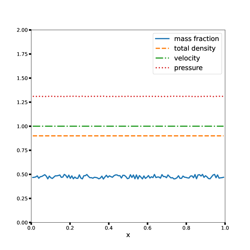
(a) $t=0$

(b) $t=0.001$

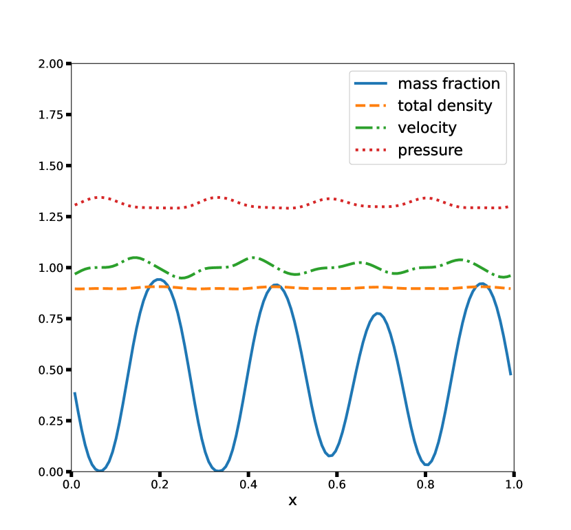
(c) $t=0.03$

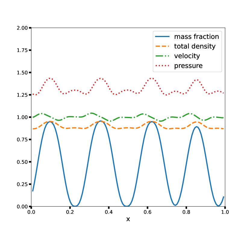
(d) $t=0.3$

Figure 1: Spatio-temporal evolution of density $\rho$, mass fraction $c$, velocity $\mathbf{v}$ and pressure $p$ for test case 1.

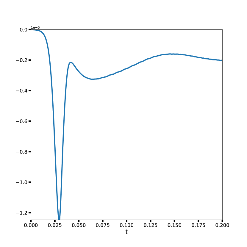
(a) Dissipation $\frac{\mathop{\kern 0.0pt\mathrm{d}}\!{}E}{\mathop{\kern 0.0pt\mathrm{d}}\!{}t}$

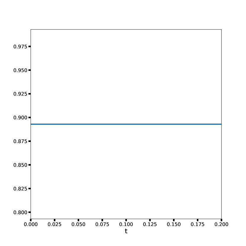
(b) Total mass

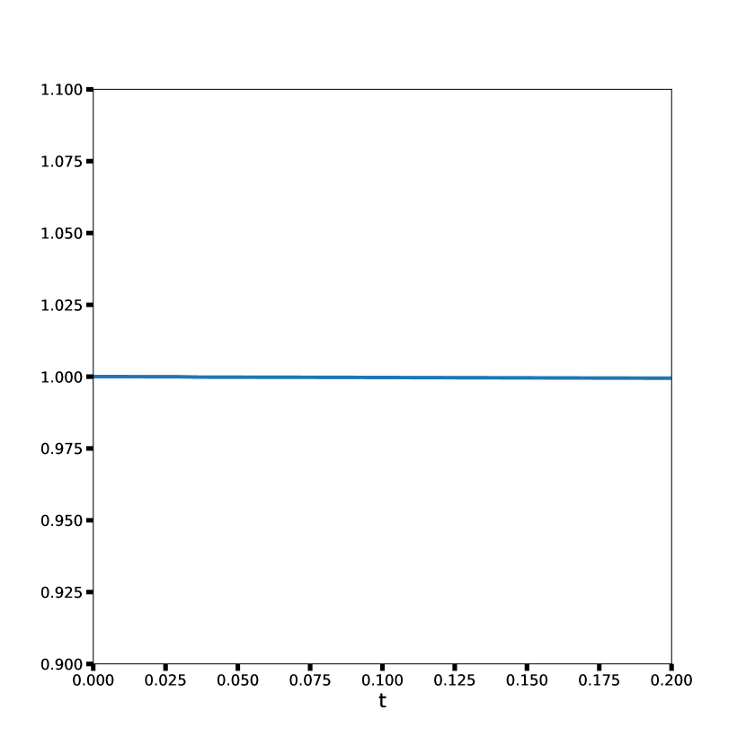
(c) Scalar variable $\xi$

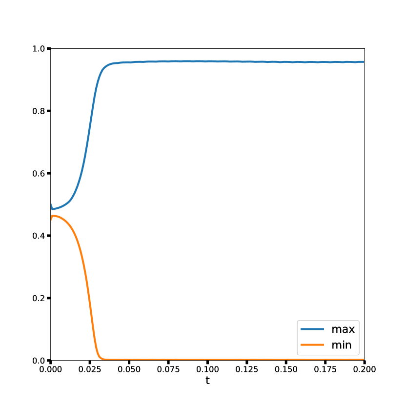
(d) minimum and maximum of $c$

Figure 2: Temporal evolution of the dissipation of the energy $\frac{\mathop{\kern 0.0pt\mathrm{d}}\!{}E}{\mathop{\kern 0.0pt\mathrm{d}}\!{}t}$, of the total mass $\int_{\Omega}\rho\,\mathop{\kern 0.0pt\mathrm{d}}\!{}x$, of the scalar variable $\xi$, and of the minimum and maximal values of the mass fraction $c$ for test case 1.

5.2 Convergence tests

We study the numerical convergence of our one dimensional scheme (4.4)–(4.16) with $\kappa(\rho,c)=0$ and $F_{c}=0$. The computational domain is $\Omega=(0,1)$. The final time is $T=0.1$ and choose $\alpha_{1}=\alpha_{2}=1$. The other parameters $\gamma$, $\beta$, $\eta$, $\nu$ are chosen as for test case 1 (see Subsection 5.1). The initial condition for the mass fraction is given by

$$c^{0}=0.5+0.01\cos(6\pi x).$$

The initial conditions for the velocity and the total density are chosen as in test case 1.

5.2.1 Convergence in space

We start by fixing the time step ${\Delta t}=1\times 10^{-5}$ and we vary the grid size. We vary the number of points $N_{x}=\{64,128,256,512,1024,2048\}$. For each ${\Delta x}$, we compute the error at time $t=T=0.1$ (we chose this value since we observed that the solution reached a stable state at that time) following

$$\text{error}=\|\rho_{\Delta x}-\rho_{{\Delta x}/2}\|+\|c_{\Delta x}-c_{{\Delta x}/2}\|+\|\mathbf{v}_{\Delta x}-\mathbf{v}_{{\Delta x}/2}\|,$$ (5.1)

in which each of the norms is computed following

$$\|\rho_{\Delta x}-\rho_{{\Delta x}/2}\|=\left({\Delta x}\sum_{j=1}^{N_{x}}\left(\rho_{\Delta x}(x_{2(j-1)+1)})-\rho_{{\Delta x}/2}(x_{j})\right)^{2}+\left(\rho_{\Delta x}((x_{2(j-1)+2)})-\rho_{{\Delta x}/2}(x_{j}))\right)^{2})\right)^{1/2},$$

with $N_{x}$ the number of points on the ${\Delta x}/2$ grid, hence, the solution on the coarse grid (i.e. ${\Delta x}/2$) is extended on the fine grid ${\Delta x}$.

We arrive at the results given in Figure 3. As expected by the upwind scheme, the spatial order of convergence is a little less than 1 for the total density $\rho$ (see Figure 3(a)) and the velocity $\mathbf{v}$ (see Figure 3(c)).

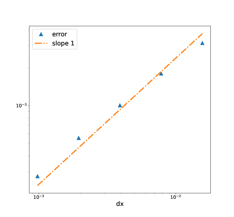
(a) Spatial convergence of density $\rho$.

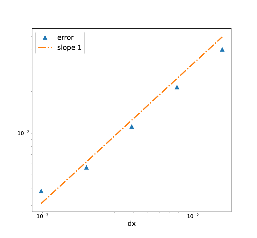
(b) Spatial convergence of mass fraction $c$.

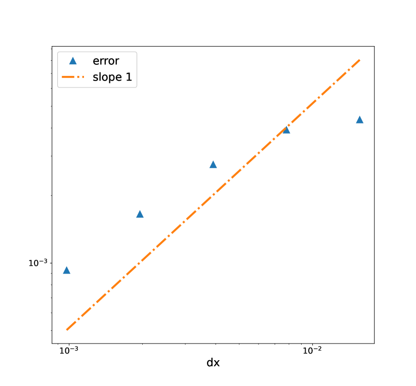
(c) Spatial convergence of velocity $\mathbf{v}$.

Figure 3: Convergence in space for the total density $\rho$, the mass fraction $c$ and the velocity $\mathbf{v}$. The orange dashed line represents the slope 1.

5.2.2 Convergence in time

We here fix the grid size and select $N_{x}=128$ points. We choose ${\Delta t}=1\times 10^{-4}$, and vary the time steps according to ${\Delta t}_{\text{array}}=\{{\Delta t},\frac{{\Delta t}}{2},\frac{{\Delta t}}{4},\frac{{\Delta t}}{8},\frac{{\Delta t}}{16},\frac{{\Delta t}}{32}\}$. The other parameters and initial conditions are chosen as in the spatial convergence test (see Subsection 5.2.1). The error between the reference solution and a computed solution at time $t=T=0.2$ is given by

$$\|\rho_{{\Delta t}}-\rho_{{\Delta t}/2}\|=\left({\Delta x}\sum_{j=1}^{N_{x}}(\rho_{{\Delta t}}(x_{j})-\rho_{{\Delta t}/2}(x_{j}))^{2}\right)^{1/2}.$$

We obtain the results depicted in Figure 4

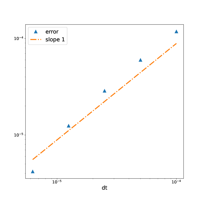
(a) Temporal convergence of density $\rho$.

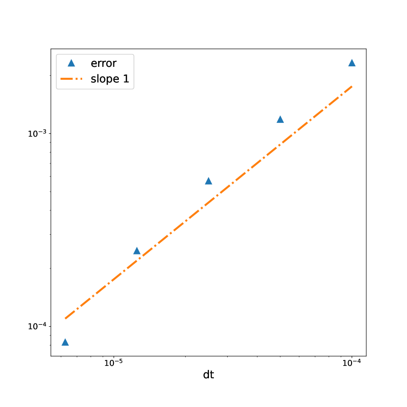
(b) Temporal convergence of mass fraction $c$.

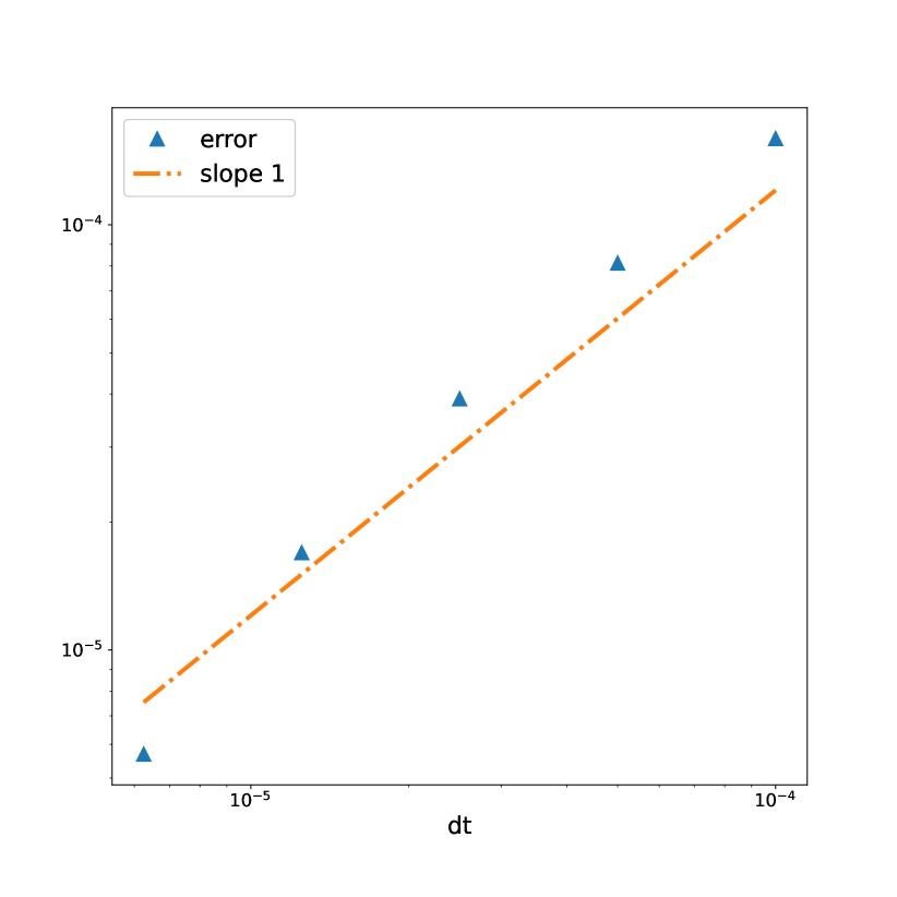
(c) Temporal convergence of velocity $\mathbf{v}$.

Figure 4: Convergence in time for the total density $\rho$, the mass fraction $c$ and the velocity $\mathbf{v}$. The orange dashed line represents the slope 1.

We observe that the order of convergence in time for our scheme is exactly $1$ as expected.

5.3 Conclusion and simulation of a growing tumor in a healthy tissue

To conclude this article, we would like to go back to our initial interest, i.e. the modeling of tumor growth. We now present a simple numerical simulation for this application and introduce a forthcoming work focusing only on the modelling of tumor.

Here, we assume that $F_{c}$ acts as a transfer of mass from the healthy tissue to the cancerous population (this can be viewed as tumor cells using material from the environment such as nutrients to divide and grow). Furthermore, we assume that the two cell populations adhere with different strengths to the ECM. Altogether, we choose

$$F_{c} =20\rho c(1-c/c^{*}),$$

$$c^{*} =0.9,$$

$$\kappa(\rho,c) =\left(\kappa_{1}\rho c+\kappa_{2}\rho(1-c)\right),\gamma=\frac{1}{1000},$$

with $c^{*}$ representing the maximum saturation (decided to be $c^{*}=1$ in the following) and $\kappa_{1}=0$ and $\kappa_{2}=20$.

For this test case, we choose the initial conditions as follows:

$$c_{0} =0.008+0.6\exp\left(-100(x-0.5)^{2}-100(y-0.5)^{2}\right),$$

$$\rho_{0} =\,c+0.5\,(1-c),$$

$$\mathbf{v}_{0} =0,$$

We chose a square domain $\Omega$ of length $1$ and $64\times 64$ cells for the spatial discretization. The other parameters that we did not specify are chosen as in Subsection 5.1.

Figs 5 show the spatio-temporal evolution of the tumor with $\alpha_{1}=\alpha_{2}=1$. We observe that as the tumor grows the shape remains radially symmetrical. We think that, due friction effects, instabilities may appear. The reason we are not able to see them in that case is double. Firstly, the scheme is less than first order in space and small structures may not be captured. Secondly, the regularization given by the double Laplacian from the Cahn-Hilliard equation may be too strong and the finger-like instabilities are not seen.

To verify the latter assertion, we propose another test case with the parameters

$$\alpha_{1}=1.2,\quad\alpha_{2}=0.8,$$

$$\kappa_{2}=100,\quad\gamma=\frac{1}{1500},$$

and

$$c_{0}=0.01+0.9\exp\left(-100(x-0.5)^{2}-100(y-0.5)^{2}\right).$$

The other parameters and the initial conditions are chosen as the previous test case.

Figs 6 show our numerical results for this "tumor growth" test case. We observe that as the tumor grows the shape does not remain perfectly symmetrical. This result emphasize that the behavior of the solution depends strongly on the regularization provided by the bi-laplacian term and the strength of the friction on the rigid fibers of the medium. Furthermore, one possible other explanation of the instabilities could be the difference of densities of between the two fluids. This is controlled by taking $\alpha_{1}\neq\alpha_{2}$ (see Figs 1 to better see one-dimensional numerical results highlighting the effect of non-matching densities). Indeed, from Figs 1 we know that taking $\alpha_{2}>\alpha_{2}$ leads to a heterogeneous pressure field which leads to pressure gradients. Hence, since the initial velocity field is zero in our case, the direction of the velocity is given by $-\nabla p$. Consequently, $\mathbf{v}$ tends to transport the cell densities to regions of less pressure, i.e. away from the tumor cell clusters. This movement in addition to heterogeneous friction effects is known to produce complex patterns (see e.g.  [47]). We argue that, from these numerical simulations, our model seems capable to qualitatively represent patterns of invasive growth of tumors and could unravel the possible mechanical effects playing a role in the emergence of heterogeneous structures observed in tumor invasion of healthy tissue.

However, we emphasize that to achieve these latter goals, we have to be able to capture accurately the possible fine structures emerging during the numerical simulations. Thus, our numerical scheme will be improved to increase the spatial and temporal orders of accuracy by taking advantage of the flexibility of the SAV method. In a forthcoming work, we will develop a high-order finite element scheme for the compressible SAV-NSCH system we proposed in the present work. This numerical scheme will allow efficient simulations of compressible diphasic fluids and will be used to simulate relevant test cases with applications in fluid mechanics such as rising bubbles and Rayleigh-Taylor instabilities.

In the previously mentioned future work, we will study the possible mechanical effects at play during invasive tumor growth. Our strategy will be relatively simple: As presented in Appendix A, we will reduce the G-NSCH system to better represent tumor growth while removing non-necessary effects such as inertia. Our goal will be to present numerical simulations capturing Saffman-Taylor-like instabilities depicted by the protrusions of the tumor in the healthy tissue and commonly observed in the context of, e.g. , skin cancer [18].

On the basis of the present work, numerous other work directions can be envisioned. Indeed, the analytical aspects of this work can be improved. This direction is challenging because as pointed out in the present work, necessary assumptions on the potential and the mobility term to perform the solutions’ existence proof do not allow to take physically or biologically relevant forms. In fact, singular potentials, degenerate mobilities and viscosity functions are not allowed. Working in this direction would require us to use recent results concerning the Cahn-Hilliard equation as well as the compressible Navier-Stokes model and adapting them to the context of the NSCH system. One possible solution that we will investigate is to derive a Bresch-Desjardins entropy estimate [12, 13] for the compressible NSCH as it has been done recently by Vasseur and Yu [60], and Bresch, Vasseur and Yu [14], for the compressible Navier-Stokes model with degenerate viscosities.

We would like to conclude this research article by presenting a possible research perspective the authors will investigate. We believe that the coupling proposed by the G-NSCH model between fluid movement and tumor growth could have an original application to the mathematical representation of tumor-on-chips [46]. Indeed, these microfluidic devices present a growing interest in oncology since they can replicate in a very accurate manner the micro-environment of the tumor. Therefore, they present a lot of advantages for experiments and the G-NSCH model could be used to replicate such experiments in an in-silico manner. We believe this could be useful to optimize the devices and also help to answer questions in oncology.

(a) Initial condition

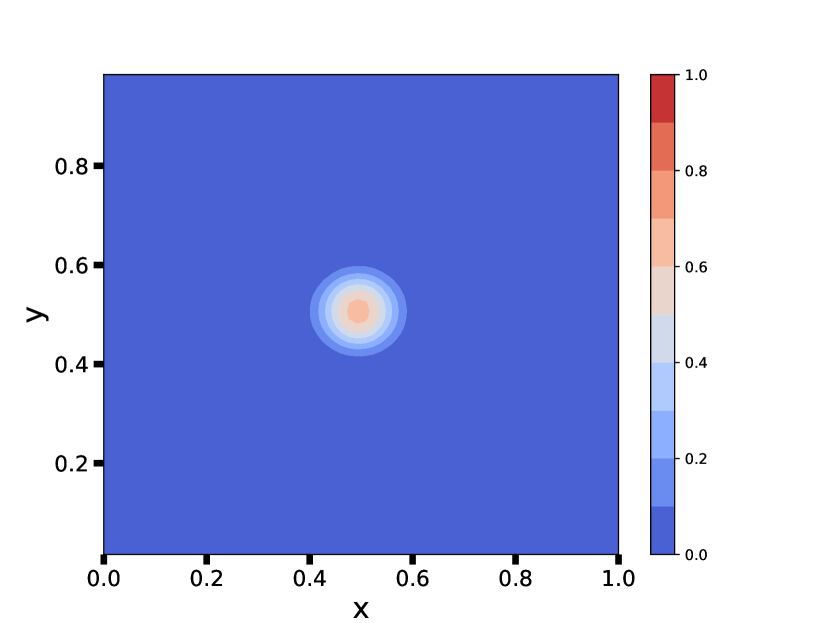
(b) $t=0.1$

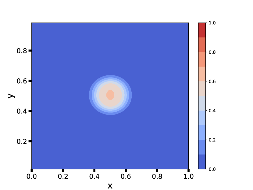
(c) $t=0.25$

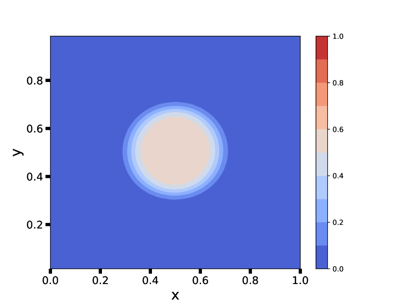
(d) $t=0.5$

Figure 5: Temporal evolution of the tumor density in the case $\alpha_{1}=\alpha_{2}$

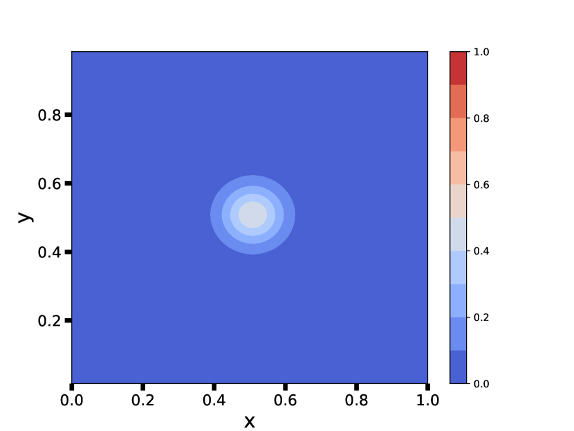
(a) Initial condition

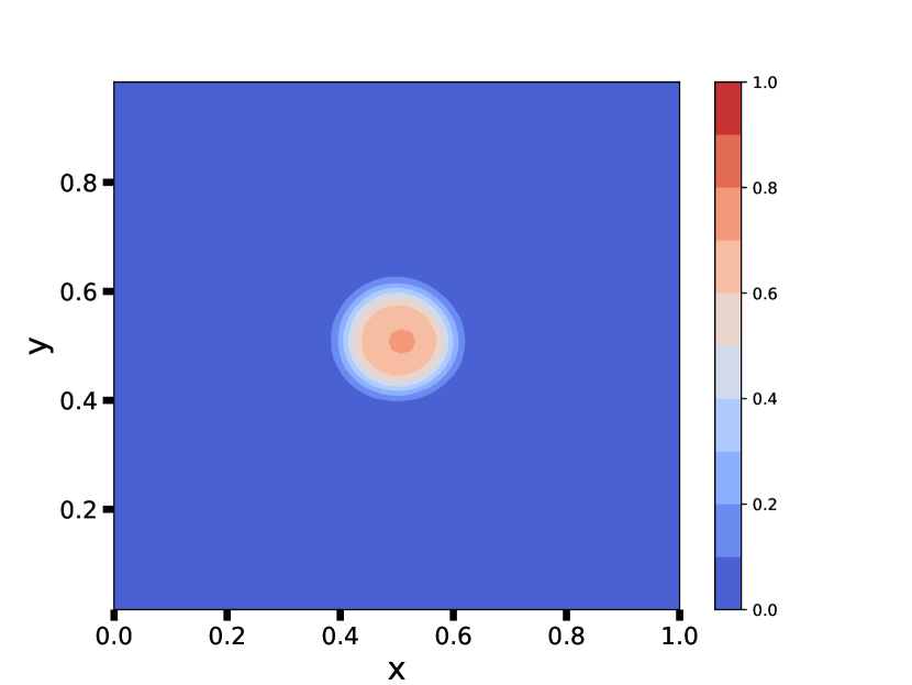
(b) $t=0.02$

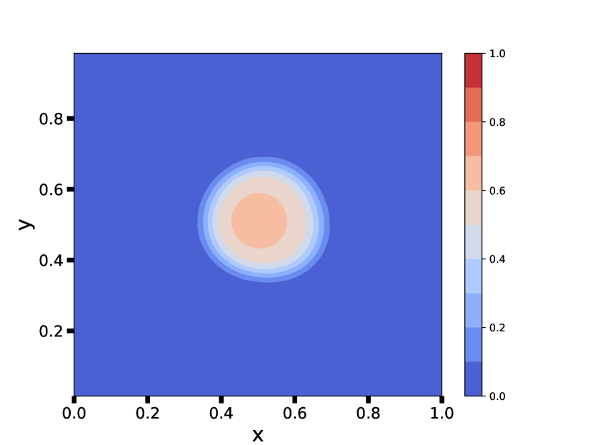
(c) $t=0.1$

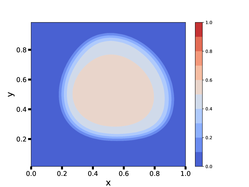
(d) $t=0.3$

Figure 6: Temporal evolution of the tumor density in the case $\alpha_{1}=0.8$ and $\alpha_{2}=1.2$.

Appendix A Derivation of the model

In this Appendix, we present the rigourous derivation of our G-NSCH model.

A.1 Notation and definitions

We formulate our problem in Eulerian coordinates and in a smooth bounded domain $\Omega\subset\mathbb{R}^{d}$ (where $d=\{1,2,3\}$ is the dimension). The balance laws derived in the following sections are in local form.

We have two cell populations in the model where $\rho_{1},\rho_{2}$ are the relative densities of respectively populations $1$ and $2$. Thus, $\rho_{i}$ represents the mass of the population $M_{i}$ per volume occupied by the $i$-th phase $V_{i}$, i.e.

$$\rho_{i}=\frac{M_{i}}{V_{i}}.$$

Then, we define the volume fractions $\varphi_{1},\varphi_{2}$ which are defined by the volume occupied by the $i$-th phase over the total volume of the mixture

$$\varphi_{i}=\frac{V_{i}}{V}.$$

Therefore, the mass density of population $i$ which is the mass of population $i$ in volume $V$ is given by

$$\phi_{i}=\rho_{i}\varphi_{i}.$$

We further assume that the fluid is saturated, i.e.

$$\varphi_{1}+\varphi_{2}=1.$$

The total density of the mixture is then given by

$$\rho=\phi_{1}+\phi_{2}.$$

We also introduce the mass fractions $c_{i}=M_{i}/M$ and we have the relations

$$\rho c_{i}=\phi_{i},\quad\text{and}\quad c_{1}=(1-c_{2}).$$ (A.1)

We denote by $p$ the pressure inside the mixture and $\mathbf{v}_{1},\mathbf{v}_{2}$ are the velocities of the different phases. We use a mass-average mixture velocity

$$\mathbf{v}=\frac{1}{\rho}\left(\phi_{1}\mathbf{v}_{1}+\phi_{2}\mathbf{v}_{2}\right).$$ (A.2)

We define the material derivative for a generic function $g$ (scalar or vector-valued) by

$$\frac{\mathop{\kern 0.0pt\mathrm{D}}\!{}g}{\mathop{\kern 0.0pt\mathrm{D}}\!{}t}=\frac{\partial g}{\partial t}+\mathbf{v}\cdot\nabla g,$$ (A.3)

and indicate the definition of the differential operator

$$\mathbf{v}\cdot\nabla g=\sum_{j=1}^{d}\mathbf{v}_{j}\frac{\partial g}{\partial x_{j}}.$$

In the following, we denote vectors with bold roman letters and we use bold Greek letters to denote second-order tensors.

A.2 Mass balance equations

We assume that each component has its own velocity and the component $1$ is proliferating. The fluid being saturated, i.e. $c_{1}+c_{2}=1$ Therefore, we have the mass balance equations for each component

$$\begin{cases}\frac{\partial\phi_{1}}{\partial t}+{\rm div}\left(\phi_{1}\mathbf{v}_{1}\right)=F_{1}(\rho,c_{1},c_{2}),\\ \frac{\partial\phi_{2}}{\partial t}+{\rm div}\left(\phi_{2}\mathbf{v}_{2}\right)=F_{2}(\rho,c_{1},c_{2}).\end{cases}$$ (A.4)

In the previous system, the functions $F_{i}(\rho,c_{1},c_{2})$ ($i=1,2$) act as source terms of mass.

Summing the two equations, we obtain the continuity equation for the total density of the mixture, and using the mass fractions (denoting $c_{1}=c$) and the relations (A.1), we obtain the balance equation for the density of the mixture

$$\frac{\partial\rho}{\partial t}+{\rm div}\left(\rho\mathbf{v}\right)=F_{1}+F_{2}=:F_{\rho}.$$ (A.5)

To obtain a system analogous to (A.4), we rewrite the first equation of (A.4) using the definition of the mass fraction (A.1) to obtain

$$\frac{\partial\rho c}{\partial t}+{\rm div}\left(\rho c\mathbf{v}_{1}\right)=F_{1}(\rho,c,1-c)=:F_{c}.$$ (A.6)

The mass of the component $1$ is transported by the average velocity $\mathbf{v}$ and the remaining diffusive flux $\mathbf{J}_{1}=\rho c\left(\mathbf{v}-\mathbf{v}_{1}\right)$. Therefore, we can replace the previous equation by

$$\frac{\partial\rho c}{\partial t}+{\rm div}\left(\rho c\mathbf{v}\right)={\rm div}\left(\mathbf{J}_{1}\right)+F_{c}.$$

Then, using the definition of the material derivative (A.3) and the mass balance equation for the total mixture (A.5), the left-hand side of the previous equation reads

$$\frac{\partial\rho c}{\partial t}+{\rm div}\left(\rho c\mathbf{v}\right)=\rho\frac{\mathop{\kern 0.0pt\mathrm{D}}\!{}c}{\mathop{\kern 0.0pt\mathrm{D}}\!{}t}+c\left[\frac{\partial\rho}{\partial t}+{\rm div}\left(\rho\mathbf{v}\right)\right]=\rho\frac{\mathop{\kern 0.0pt\mathrm{D}}\!{}c}{\mathop{\kern 0.0pt\mathrm{D}}\!{}t}+cF_{\rho}.$$

Altogether, we obtain the balance equation for the mass fraction of the component $1$

$$\rho\frac{\mathop{\kern 0.0pt\mathrm{D}}\!{}c}{\mathop{\kern 0.0pt\mathrm{D}}\!{}t}={\rm div}\left(\mathbf{J}_{1}\right)+F_{c}-cF_{\rho}.$$ (A.7)

Since $c_{2}=1-c$, solving the equations (A.5) and (A.7) is equivalent to solving the system (A.4). In the following, we refer to $c$ as the order parameter (terminology often used in the framework of the Cahn-Hilliard model [17, 16]).

A.3 Balance of linear momentum

We write the balance of linear momentum [22], which describes the evolution of the velocity $\mathbf{v}$ due to internal stresses. Indeed, we neglect the effect of any external forces, including gravity. Following continuum mechanics, the Cauchy stress tensor gives the stresses acting inside the mixture due to viscous and non-viscous effects. An additional stress must be taken into account to represent the effect of concentration gradients [24]. Altogether, we assume that the stress tensor is a function of the total density $\rho$, the order parameter $c$ (i.e. the mass fraction of population $1$), its gradient $\nabla c$, and the total velocity of the mixture $\mathbf{v}$ i.e.

$$\boldsymbol{\sigma}=\boldsymbol{\sigma}(\rho,c,\nabla c,\mathbf{v}).$$

The friction around the pores of the medium is modeled by a drag term in the balance equation [54] with a permeability coefficient $\kappa(\rho,c)=\kappa_{1}(\rho,c)+\kappa_{2}(\rho,c)$ (the sum of the two friction coefficients for each component of the mixture). The permeability coefficient relates the properties of the fluid and the porous medium.

For each dimension (for example if $d=3$, then $j=\{x,y,z\}$), the balance of linear momentum reads [22]

$$\frac{\partial\rho\mathbf{v}_{j}}{\partial t}+{\rm div}\left(\rho\mathbf{v}_{j}\mathbf{v}\right)={\rm div}\left(\boldsymbol{\sigma}\right)_{j}-\kappa(\rho,c)\mathbf{v}_{j}+F_{\mathbf{v}_{j}},$$

where $F_{\mathbf{v}_{j}}(\mathbf{v}_{j},\rho)$ represents the gain or loss of velocity in the $j$-th direction from different effects such as external forces. Then, using the continuity equation (A.5), we can rearrange the left-hand side to obtain

$$\frac{\partial\rho\mathbf{v}_{j}}{\partial t}+{\rm div}\left(\rho\mathbf{v}_{j}\mathbf{v}\right)=\rho\frac{\mathop{\kern 0.0pt\mathrm{D}}\!{}\mathbf{v}_{j}}{\mathop{\kern 0.0pt\mathrm{D}}\!{}t}+\mathbf{v}_{j}\left[\frac{\partial\rho}{\partial t}+{\rm div}\left(\rho\mathbf{v}\right)\right]=\rho\frac{\mathop{\kern 0.0pt\mathrm{D}}\!{}\mathbf{v}_{j}}{\mathop{\kern 0.0pt\mathrm{D}}\!{}t}+\mathbf{v}_{j}F_{\rho}+F_{\mathbf{v}_{j}}.$$

Therefore, we have

$$\rho\frac{\mathop{\kern 0.0pt\mathrm{D}}\!{}\mathbf{v}_{j}}{\mathop{\kern 0.0pt\mathrm{D}}\!{}t}={\rm div}(\boldsymbol{\sigma})_{j}-\left(\kappa(\rho,c)+F_{\rho}\right)\mathbf{v}_{j}+F_{\mathbf{v}_{j}}.$$

Then, we can rewrite the balance of linear momentum in a more compact form

$$\rho\frac{\mathop{\kern 0.0pt\mathrm{D}}\!{}\mathbf{v}}{\mathop{\kern 0.0pt\mathrm{D}}\!{}t}={\rm div}(\boldsymbol{\sigma})-\left(\kappa(\rho,c)+F_{\rho}\right)\mathbf{v}+F_{\mathbf{v}},$$ (A.8)

where $F_{\mathbf{v}}(\mathbf{v},\rho)$ is the vector of coordinates $F_{\mathbf{v}_{j}}$.

A.4 Energy balance

The total energy of the mixture is the sum of the kinetic energy $\rho\frac{1}{2}\lvert\mathbf{v}\rvert^{2}$ and of the internal energy $\rho u$, where $u=u(\rho,c,\nabla c)$ is a specific internal energy. Compared to the classical conservation law for the total energy, we have an additional energy flux $\boldsymbol{\tau}\frac{\mathop{\kern 0.0pt\mathrm{D}}\!{}c}{\mathop{\kern 0.0pt\mathrm{D}}\!{}t}$. Indeed, due to the interface region, surface effects must be taken into account. Following this direction, Gurtin [30] proposed to include in the second law of thermodynamics, the effect of an additional force called the microscopic-stress which is related to forces acting at the microscopic scale. We denote this supplementary stress by $\boldsymbol{\tau}$.

Since we assume that the system is maintained in an isothermal state, the balance equation for the energy is given by [22]

$$\frac{\partial}{\partial t}\left(\rho\frac{1}{2}\lvert\mathbf{v}\rvert^{2}+\rho u\right) +{\rm div}\left(\rho\left(\frac{1}{2}\lvert\mathbf{v}\rvert^{2}+u\right)\mathbf{v}\right)$$ (A.9)

$$={\rm div}\left(\boldsymbol{\sigma}^{T}\mathbf{v}\right)+{\rm div}\left(\boldsymbol{\tau}\frac{\mathop{\kern 0.0pt\mathrm{D}}\!{}c}{\mathop{\kern 0.0pt\mathrm{D}}\!{}t}\right)-{\rm div}\left(\mathbf{q}\right)+\rho g+c_{\rho}F_{\rho}+c_{c}F_{c}+c_{\mathbf{v}}F_{\mathbf{v}},$$

where $\mathbf{q}$ is the heat flux and $\rho g$ is the density of heat sources to maintain the temperature constant. The last three terms in Equation (A.9) account for the energy supply coming from the mass and velocity sources (see e.g.  [31, 40]). The prefactors $c_{\rho},c_{c},c_{\mathbf{v}}$ will be determined later to satisfy the free energy imbalance. Then, repeating the same calculations on the left-hand side to use the balance of mass (A.5), we get

$$\frac{\partial}{\partial t}\left(\rho\frac{1}{2}\lvert\mathbf{v}\rvert^{2}+\rho u\right)+{\rm div}\left(\rho\left(\frac{1}{2}\lvert\mathbf{v}\rvert^{2}+u\right)\mathbf{v}\right)=\rho\left[\frac{\mathop{\kern 0.0pt\mathrm{D}}\!{}}{\mathop{\kern 0.0pt\mathrm{D}}\!{}t}\left(\frac{1}{2}\lvert\mathbf{v}\rvert^{2}+u\right)\right]+\left(\frac{1}{2}\lvert\mathbf{v}\rvert^{2}+u\right)F_{\rho}.$$

Applying the chain rule to the kinetic part, we get

$$\rho\frac{\mathop{\kern 0.0pt\mathrm{D}}\!{}}{\mathop{\kern 0.0pt\mathrm{D}}\!{}t}\left(\frac{1}{2}\lvert\mathbf{v}\rvert^{2}\right)=\rho\mathbf{v}\cdot\frac{\mathop{\kern 0.0pt\mathrm{D}}\!{}\mathbf{v}}{\mathop{\kern 0.0pt\mathrm{D}}\!{}t},$$

and using the balance of linear momentum (A.8), we obtain

$$\rho\mathbf{v}\cdot\frac{\mathop{\kern 0.0pt\mathrm{D}}\!{}\mathbf{v}}{\mathop{\kern 0.0pt\mathrm{D}}\!{}t}=\mathbf{v}\cdot{\rm div}(\boldsymbol{\sigma})-\left(\kappa(\rho,c)+F_{\rho}\right)\lvert\mathbf{v}\rvert^{2}+F_{\mathbf{v}}\cdot\mathbf{v}.$$

Using these previous equations inside (A.9), we obtain the balance equation for the internal energy

$$\rho\frac{\mathop{\kern 0.0pt\mathrm{D}}\!{}u}{\mathop{\kern 0.0pt\mathrm{D}}\!{}t}={\rm div}\left(\boldsymbol{\sigma}^{T}\mathbf{v}\right)-\mathbf{v}\cdot{\rm div}\left(\boldsymbol{\sigma}\right) +{\rm div}\left(\boldsymbol{\tau}\frac{\mathop{\kern 0.0pt\mathrm{D}}\!{}c}{\mathop{\kern 0.0pt\mathrm{D}}\!{}t}\right)+\left(\kappa(\rho,c)+F_{\rho}\right)\lvert\mathbf{v}\rvert^{2}-F_{v}\mathbf{v}$$

$$-{\rm div}\left(\mathbf{q}\right)+\rho g-\left(\frac{1}{2}\lvert\mathbf{v}\rvert^{2}+u\right)F_{\rho}+c_{\rho}F_{\rho}+c_{c}F_{c}+c_{\mathbf{v}}F_{\mathbf{v}}.$$

However, since

$$\mathbf{v}\cdot\left({\rm div}\left(\boldsymbol{\sigma}\right)\right)-{\rm div}\left(\boldsymbol{\sigma}^{T}\mathbf{v}\right)=-\boldsymbol{\sigma}\mathbin{\vbox{\hbox{$\ldotp$}\hbox{$\ldotp$}}}\nabla\mathbf{v},$$

where $\nabla\mathbf{v}=\left(\partial_{x_{j}}\mathbf{v}_{i}\right)_{i,j=1,\dots,d}$ is the Jacobi matrix and, we have ${A\mathbin{\vbox{\hbox{$\ldotp$}\hbox{$\ldotp$}}}B=\sum_{i,j}A_{ij}B_{ij}}$, for two matrices $A,B$. Altogether, we have the balance equation for the internal energy

$$\rho\frac{\mathop{\kern 0.0pt\mathrm{D}}\!{}u}{\mathop{\kern 0.0pt\mathrm{D}}\!{}t}=\boldsymbol{\sigma}\mathbin{\vbox{\hbox{$\ldotp$}\hbox{$\ldotp$}}}\nabla\mathbf{v} +{\rm div}\left(\boldsymbol{\tau}\frac{\mathop{\kern 0.0pt\mathrm{D}}\!{}c}{\mathop{\kern 0.0pt\mathrm{D}}\!{}t}\right)+\left(\kappa(\rho,c)+F_{\rho}\right)\lvert\mathbf{v}\rvert^{2}-F_{v}\mathbf{v}$$ (A.10)

$$-{\rm div}\left(\mathbf{q}\right)+\rho g-\left(\frac{1}{2}\lvert\mathbf{v}\rvert^{2}+u\right)F_{\rho}+c_{\rho}F_{\rho}+c_{c}F_{c}+c_{\mathbf{v}}F_{\mathbf{v}}.$$

A.5 Entropy balance and Clausius-Duhem inequality

We aim to apply the second law of thermodynamics. To do so, we define the entropy $s=s(\rho,c,\nabla c)$ and the Helmholtz free energy $\mathcal{F}=\mathcal{F}(\rho,c,\nabla c)$, both related through the equation

$$\mathcal{F}=u-Ts,$$ (A.11)

where $T$ denotes the temperature.

From the mass balance equation (A.5), we have the entropy balance equation

$$\frac{\partial\rho s}{\partial t}+{\rm div}(s\rho\mathbf{v})=\rho\frac{\mathop{\kern 0.0pt\mathrm{D}}\!{}s}{\mathop{\kern 0.0pt\mathrm{D}}\!{}t}+s\left[\frac{\partial\rho}{\partial t}+{\rm div}\left(\rho\mathbf{v}\right)\right]=\rho\frac{\mathop{\kern 0.0pt\mathrm{D}}\!{}s}{\mathop{\kern 0.0pt\mathrm{D}}\!{}t}+sF_{\rho}.$$ (A.12)

Then, using the definition of the Helmholtz free energy (A.11) and the balance of energy (A.10), we obtain

$$\rho\frac{\mathop{\kern 0.0pt\mathrm{D}}\!{}s}{\mathop{\kern 0.0pt\mathrm{D}}\!{}t} =-\frac{\rho}{T}\frac{\mathop{\kern 0.0pt\mathrm{D}}\!{}\mathcal{F}}{\mathop{\kern 0.0pt\mathrm{D}}\!{}t}+\frac{\rho}{T}\frac{\mathop{\kern 0.0pt\mathrm{D}}\!{}u}{\mathop{\kern 0.0pt\mathrm{D}}\!{}t}$$ (A.13)

$$=-\frac{\rho}{T}\frac{\mathop{\kern 0.0pt\mathrm{D}}\!{}\mathcal{F}}{\mathop{\kern 0.0pt\mathrm{D}}\!{}t}+\begin{multlined}\frac{1}{T}\big{[}\boldsymbol{\sigma}\mathbin{\vbox{\hbox{$\ldotp$}\hbox{$\ldotp$}}}\nabla\mathbf{v}+{\rm div}\left(\boldsymbol{\tau}\frac{\mathop{\kern 0.0pt\mathrm{D}}\!{}c}{\mathop{\kern 0.0pt\mathrm{D}}\!{}t}\right)+\left(\kappa(\rho,c)+F_{\rho}\right)\lvert\mathbf{v}\rvert^{2}-F_{v}\mathbf{v}\\ -{\rm div}\left(\mathbf{q}\right)+\rho g-\left(\frac{1}{2}\lvert\mathbf{v}\rvert^{2}+u\right)F_{\rho}+c_{\rho}F_{\rho}+c_{c}F_{c}+c_{\mathbf{v}}F_{\mathbf{v}}\big{]},\end{multlined}\frac{1}{T}\big{[}\boldsymbol{\sigma}\mathbin{\vbox{\hbox{$\ldotp$}\hbox{$\ldotp$}}}\nabla\mathbf{v}+{\rm div}\left(\boldsymbol{\tau}\frac{\mathop{\kern 0.0pt\mathrm{D}}\!{}c}{\mathop{\kern 0.0pt\mathrm{D}}\!{}t}\right)+\left(\kappa(\rho,c)+F_{\rho}\right)\lvert\mathbf{v}\rvert^{2}-F_{v}\mathbf{v}\\ -{\rm div}\left(\mathbf{q}\right)+\rho g-\left(\frac{1}{2}\lvert\mathbf{v}\rvert^{2}+u\right)F_{\rho}+c_{\rho}F_{\rho}+c_{c}F_{c}+c_{\mathbf{v}}F_{\mathbf{v}}\big{]},$$

where we have replaced the material derivative of the internal energy using its balance equation (A.10).

The constitutive relations for the functions constituting the Navier-Stokes-Cahn-Hilliard model are often derived to satisfy the Clausius-Duhem inequality (Coleman-Noll Procedure) [22]. Indeed, this inequality provides a set of restrictions for the dissipative mechanisms occurring in the system. However, in our case, due to the presence of source terms, we can not ensure that this inequality holds without some assumptions on the proliferation and friction of the fluid around the pores. Therefore, we use here a different method: the Lagrange multipliers method. Indeed, the Liu [45] and Müller [53] method is based on using Lagrange multipliers to derive a set of restrictions on the constitutive relations that can be applied even in the presence of source terms.

Following classical Thermodynamics [53], we state the second law as an entropy inequality, i.e., the Clausius-Duhem inequality in the local form [22]

$$\rho\frac{\mathop{\kern 0.0pt\mathrm{D}}\!{}s}{\mathop{\kern 0.0pt\mathrm{D}}\!{}t}\geq-{\rm div}\left(\frac{\mathbb{q}}{T}\right)+\frac{\rho g}{T}+{\rm div}\left(\mathcal{J}\right),$$ (A.14)

where $\mathcal{J}$ is the entropy flux. The inequality (A.14) results from the fact that the entropy of the mixture can only increase. Using the equation (A.13), we obtain

$$\frac{\rho}{T}\frac{D\mathcal{F}}{Dt}-\frac{1}{T}\big{[} \boldsymbol{\sigma}\mathbin{\vbox{\hbox{$\ldotp$}\hbox{$\ldotp$}}}\nabla\mathbf{v}+{\rm div}\left(\boldsymbol{\tau}\frac{\mathop{\kern 0.0pt\mathrm{D}}\!{}c}{\mathop{\kern 0.0pt\mathrm{D}}\!{}t}\right)+\left(\kappa(\rho,c)+F_{\rho}\right)\lvert\mathbf{v}\rvert^{2}$$ (A.15)

$$-F_{v}\mathbf{v}-\left(\frac{1}{2}\lvert\mathbf{v}\rvert^{2}+u\right)F_{\rho}+c_{\rho}F_{\rho}+c_{c}F_{c}+c_{\mathbf{v}}F_{\mathbf{v}}\big{]}+{\rm div}\left(\mathcal{J}\right)\leq 0.$$

Then, using the chain rule

$$\frac{D\mathcal{F}}{Dt}=\frac{D\rho}{Dt}\frac{\partial\mathcal{F}}{\partial\rho}+\frac{Dc}{Dt}\frac{\partial\mathcal{F}}{\partial c}+\frac{D\nabla c}{Dt}\cdot\frac{\partial\mathcal{F}}{\partial\nabla c},$$

and

$$\frac{D\nabla c}{Dt}=\nabla\left[\frac{Dc}{Dt}\right]-\left(\nabla\mathbf{v}\right)^{T}\nabla c,\quad\frac{\mathop{\kern 0.0pt\mathrm{D}}\!{}\rho}{\mathop{\kern 0.0pt\mathrm{D}}\!{}t}=-\rho{\rm div}(\mathbf{v})+F_{\rho},$$

in the entropy inequality (A.15), we obtain

$$\rho \left[\left(-\rho{\rm div}(\mathbf{v})+F_{\rho}\right)\frac{\partial\mathcal{F}}{\partial\rho}+\frac{\mathop{\kern 0.0pt\mathrm{D}}\!{}c}{\mathop{\kern 0.0pt\mathrm{D}}\!{}t}\frac{\partial\mathcal{F}}{\partial c}+\left(\nabla\left[\frac{Dc}{Dt}\right]-\left(\nabla\mathbf{v}\right)^{T}\nabla c\right)\cdot\frac{\partial\mathcal{F}}{\partial\nabla c}\right]-{\rm div}\left(\boldsymbol{\tau}\frac{\mathop{\kern 0.0pt\mathrm{D}}\!{}c}{\mathop{\kern 0.0pt\mathrm{D}}\!{}t}\right)-\sigma:\nabla\mathbf{v}$$ (A.16)

$$-\left[\left(\kappa(\rho,c)+F_{\rho}\right)\lvert\mathbf{v}\rvert^{2}-F_{v}\mathbf{v}-\left(\frac{1}{2}\lvert\mathbf{v}\rvert^{2}+u\right)F_{\rho}+c_{\rho}F_{\rho}+c_{c}F_{c}+c_{\mathbf{v}}F_{\mathbf{v}}\right]+T{\rm div}\left(\mathcal{J}\right)\leq 0.$$

By the chain rule, we have

$${\rm div}\left(\boldsymbol{\tau}\frac{\mathop{\kern 0.0pt\mathrm{D}}\!{}c}{\mathop{\kern 0.0pt\mathrm{D}}\!{}t}\right)=\boldsymbol{\tau}\nabla\left[\frac{Dc}{Dt}\right]+\frac{\mathop{\kern 0.0pt\mathrm{D}}\!{}c}{\mathop{\kern 0.0pt\mathrm{D}}\!{}t}{\rm div}\left(\boldsymbol{\tau}\right).$$

Furthermore, we know that

$$-\rho^{2}{\rm div}\left(\mathbf{v}\right)\frac{\partial\mathcal{F}}{\partial\rho}=-\rho^{2}\frac{\partial\mathcal{F}}{\partial\rho}\mathbf{1}\mathbin{\vbox{\hbox{$\ldotp$}\hbox{$\ldotp$}}}\nabla\mathbf{v},$$

and

$$-\rho\left(\left(\nabla\mathbf{v}\right)^{T}\nabla c\right)\cdot\frac{\partial\mathcal{F}}{\partial\nabla c}=-\rho\left(\nabla c\otimes\frac{\partial\mathcal{F}}{\partial\nabla c}\right)\mathbin{\vbox{\hbox{$\ldotp$}\hbox{$\ldotp$}}}\nabla\mathbf{v}.$$

Gathering the previous three relations and reorganizing the terms of (A.16), we obtain

$$\left(-\rho^{2}\frac{\partial\mathcal{F}}{\partial\rho}\mathbf{1}-\rho\nabla c\otimes\frac{\partial\mathcal{F}}{\partial\nabla c}-\boldsymbol{\sigma}\right)\mathbin{\vbox{\hbox{$\ldotp$}\hbox{$\ldotp$}}}\nabla\mathbf{v}+\left(\rho\frac{\partial\mathcal{F}}{\partial c}-{\rm div}(\boldsymbol{\tau})\right)\frac{\mathop{\kern 0.0pt\mathrm{D}}\!{}c}{\mathop{\kern 0.0pt\mathrm{D}}\!{}t}$$ (A.17)

$$+\left(\rho\frac{\partial\mathcal{F}}{\partial\nabla c}-\boldsymbol{\tau}\right)\nabla\left[\frac{\mathop{\kern 0.0pt\mathrm{D}}\!{}c}{\mathop{\kern 0.0pt\mathrm{D}}\!{}t}\right]+T{\rm div}\left(\mathcal{J}\right)$$

$$-\left[\left(\kappa(\rho,c)+F_{\rho}\right)\lvert\mathbf{v}\rvert^{2}-F_{v}\mathbf{v}-\left(\frac{1}{2}\lvert\mathbf{v}\rvert^{2}+u-\rho\frac{\partial\mathcal{F}}{\partial\rho}\right)F_{\rho}+c_{\rho}F_{\rho}+c_{c}F_{c}+c_{\mathbf{v}}F_{\mathbf{v}}\right]\leq 0.$$

Then, we use Liu’s Lagrange multipliers method [45]. We denote by $L_{c}$ the Lagrange multiplier associated with the mass fraction equation (A.7). The method of Lagrange multipliers consists in setting the following local dissipation inequality that has to hold for arbitrary values of $(\rho,c,\nabla\rho,\nabla c,\mathbf{v},p)$

$$-D_{\text{iss}}:= \left(-\rho^{2}\frac{\partial\mathcal{F}}{\partial\rho}\mathbf{1}-\rho\nabla c\otimes\frac{\partial\mathcal{F}}{\partial\nabla c}-\boldsymbol{\sigma}\right)\mathbin{\vbox{\hbox{$\ldotp$}\hbox{$\ldotp$}}}\nabla\mathbf{v}$$ (A.18)

$$+\left(\rho\frac{\partial\mathcal{F}}{\partial c}-{\rm div}(\boldsymbol{\tau})\right)\frac{\mathop{\kern 0.0pt\mathrm{D}}\!{}c}{\mathop{\kern 0.0pt\mathrm{D}}\!{}t}+\left(\rho\frac{\partial\mathcal{F}}{\partial\nabla c}-\boldsymbol{\tau}\right)\nabla\left[\frac{\mathop{\kern 0.0pt\mathrm{D}}\!{}c}{\mathop{\kern 0.0pt\mathrm{D}}\!{}t}\right]+T{\rm div}\left(\mathcal{J}\right)$$

$$-\left[\left(\kappa(\rho,c)+F_{\rho}\right)\lvert\mathbf{v}\rvert^{2}-F_{v}\mathbf{v}-\left(\frac{1}{2}\lvert\mathbf{v}\rvert^{2}+u-\rho\frac{\partial\mathcal{F}}{\partial\rho}\right)F_{\rho}+c_{\rho}F_{\rho}+c_{c}F_{c}+c_{\mathbf{v}}F_{\mathbf{v}}\right]$$

$$-L_{c}\left(\rho\frac{\mathop{\kern 0.0pt\mathrm{D}}\!{}c}{\mathop{\kern 0.0pt\mathrm{D}}\!{}t}-{\rm div}\left(\mathbf{J}_{1}\right)-F_{c}-cF_{\rho}\right)\leq 0.$$

Since,

$${\rm div}\left(L_{c}\mathbf{J}_{1}\right)=L_{c}{\rm div}\left(\mathbf{J}_{1}\right)+\nabla L_{c}\cdot\mathbf{J}_{1},$$

we reorganize the terms of (A.18) to obtain

$$-D_{\text{iss}}:= \left(-\rho^{2}\frac{\partial\mathcal{F}}{\partial\rho}\mathbf{1}-\rho\nabla c\otimes\frac{\partial\mathcal{F}}{\partial\nabla c}-\boldsymbol{\sigma}\right)\mathbin{\vbox{\hbox{$\ldotp$}\hbox{$\ldotp$}}}\nabla\mathbf{v}$$ (A.19)

$$+\left(\rho\frac{\partial\mathcal{F}}{\partial c}-{\rm div}(\boldsymbol{\tau})-\rho L_{c}\right)\frac{\mathop{\kern 0.0pt\mathrm{D}}\!{}c}{\mathop{\kern 0.0pt\mathrm{D}}\!{}t}+\left(\rho\frac{\partial\mathcal{F}}{\partial\nabla c}-\boldsymbol{\tau}\right)\nabla\left[\frac{\mathop{\kern 0.0pt\mathrm{D}}\!{}c}{\mathop{\kern 0.0pt\mathrm{D}}\!{}t}\right]+{\rm div}\left(T\mathcal{J}+L_{c}\mathbf{J}_{1}\right)$$

$$-\nabla L_{c}\cdot\mathbf{J}_{1}$$

$$\begin{multlined}-\big{[}\left(\kappa(\rho,c)+F_{\rho}\right)\lvert\mathbf{v}\rvert^{2}-F_{v}\mathbf{v}-\left(\frac{1}{2}\lvert\mathbf{v}\rvert^{2}+u-\rho\frac{\partial\mathcal{F}}{\partial\rho}\right)F_{\rho}\\ +c_{\rho}F_{\rho}+c_{c}F_{c}+c_{\mathbf{v}}F_{\mathbf{v}}+L_{c}(F_{c}+cF_{\rho})\big{]}\leq 0.\end{multlined}-\big{[}\left(\kappa(\rho,c)+F_{\rho}\right)\lvert\mathbf{v}\rvert^{2}-F_{v}\mathbf{v}-\left(\frac{1}{2}\lvert\mathbf{v}\rvert^{2}+u-\rho\frac{\partial\mathcal{F}}{\partial\rho}\right)F_{\rho}\\ +c_{\rho}F_{\rho}+c_{c}F_{c}+c_{\mathbf{v}}F_{\mathbf{v}}+L_{c}(F_{c}+cF_{\rho})\big{]}\leq 0.$$

A.6 Constitutive assumptions and model equations

First of all, we assume that the free energy density $\mathcal{F}$ is of Ginzburg-Landau type and has the following form [17, 16]

$$\mathcal{F}(\rho,c,\nabla c)\coloneqq\psi_{0}(\rho,c)+\frac{\gamma}{2}\lvert\nabla c\rvert^{2},$$ (A.20)

where $\psi_{0}$ is the homogeneous free energy accounting for the processes of phase separation and the gradient term $\frac{\gamma}{2}\lvert\nabla c\rvert^{2}$ represents the surface tension between the two phases. This free energy is the basis of the Cahn-Hilliard model which describes the phase separation occurring in binary mixtures. Furthermore, as obtained in Wise et al.  [61], the adhesion energy between different cell species is indeed well represented by such a choice of the free energy functional.

To satisfy the inequality (A.19), we first choose

$$\boldsymbol{\tau}\coloneqq\rho\frac{\partial\mathcal{F}}{\partial\nabla c}=\gamma\rho\nabla c.$$

Then, we define the chemical potential $\mu(\rho,c,\nabla c)$ by

$$\mu\coloneqq\frac{\partial\mathcal{F}}{\partial c}-\frac{1}{\rho}{\rm div}(\boldsymbol{\tau})=\frac{\partial\mathcal{F}}{\partial c}-\frac{1}{\rho}{\rm div}(\rho\frac{\partial\mathcal{F}}{\partial\nabla c})=\frac{\partial\psi_{0}}{\partial c}-\frac{\gamma}{\rho}{\rm div}\left(\rho\nabla c\right),$$

which in turn gives a condition for the Lagrange multiplier

$$L_{c}=\mu.$$ (A.21)

Using these previous constitutive relations, we have already canceled some terms in the entropy inequality

$$\left(\rho\frac{\partial\mathcal{F}}{\partial c}-{\rm div}(\boldsymbol{\tau})-\rho L_{c}\right)\frac{\mathop{\kern 0.0pt\mathrm{D}}\!{}c}{\mathop{\kern 0.0pt\mathrm{D}}\!{}t}+\left(\rho\frac{\partial\mathcal{F}}{\partial\nabla c}-\boldsymbol{\tau}\right)\nabla\left[\frac{\mathop{\kern 0.0pt\mathrm{D}}\!{}c}{\mathop{\kern 0.0pt\mathrm{D}}\!{}t}\right]=0.$$

Then, using classical results on isothermal diffusion [50, 22], we have

$$\mathcal{J}\coloneqq-\frac{\mu\mathbf{J}_{1}}{T},$$ (A.22)

and using a generalized Fick’s law, we have

$$\mathbf{J}_{1}\coloneqq b(c)\nabla\mu,$$ (A.23)

where $b(c)$ is a nonnegative mobility function that we will specify in the following. The two constitutive relations for the diffusive fluxes (A.22) and (A.23) together with (A.21), we obtain

$${\rm div}\left(T\mathcal{J}+L_{c}\mathbf{J}_{1}\right)-\nabla L_{c}\cdot\mathbf{J}_{1}=-b(c)\lvert\nabla\mu\rvert^{2}\leq 0.$$

Following [50, 4], we define the pressure inside the mixture by

$$p\coloneqq\rho^{2}\frac{\partial\psi_{0}}{\partial\rho}.$$ (A.24)

From standard rheology, we assume that the fluid meets Newton’s rheological laws. The stress tensor is composed of two parts for the viscous $\tilde{\mathbf{P}}$ and non-viscous $\mathbf{P}$ contributions of stress

$$\boldsymbol{\sigma}\coloneqq\mathbf{P}+\tilde{\mathbf{P}},$$ (A.25)

and we have by standard continuum mechanics (see e.g.  [10, 22, 4])

$$\begin{cases}\mathbf{P}=-\left(p-\frac{\gamma}{2}\lvert\nabla c\rvert^{2}\right)\mathbf{1}-\gamma\rho\nabla c\otimes\nabla c,\\ \tilde{\mathbf{P}}=\nu(c)\left(\nabla\mathbf{v}+\nabla\mathbf{v}^{T}\right)+\lambda(c)\left({\rm div}\left(\mathbf{v}\right)\right)\mathbf{1}.\end{cases}$$ (A.26)

The second term in the non-viscous part of the stress (namely $-\gamma\left(\rho\nabla c\otimes\nabla c\right)$) is representing capillary stresses that act at the interface of the two populations. Furthermore, we assume that the bulk viscosity is zero and, consequently, we set $\lambda(c)=-\frac{2}{3}\nu(c)$. This form for the stress tensor is also the same used for Navier-Stokes fluids [24].

Using (A.26), we can cancel a new term in (A.19)

$$\left(-\rho^{2}\frac{\partial\mathcal{F}}{\partial\rho}\mathbf{1}-\rho\nabla c\otimes\frac{\partial\mathcal{F}}{\partial\nabla c}-\boldsymbol{\sigma}\right)\mathbin{\vbox{\hbox{$\ldotp$}\hbox{$\ldotp$}}}\nabla\mathbf{v}=0.$$

Therefore, the remaining terms of the entropy inequality are the ones associated with proliferation and friction. The last step to satisfy the entropy inequality is to choose arbitrarily a value for the Lagrange multiplier $c_{\rho}$, such that

$$-\big{[}\left(\kappa(\rho,c)+F_{\rho}\right)\lvert\mathbf{v}\rvert^{2} -F_{v}\mathbf{v}-\left(\frac{1}{2}\lvert\mathbf{v}\rvert^{2}+u-\rho\frac{\partial\mathcal{F}}{\partial\rho}\right)F_{\rho}$$

$$+c_{\rho}F_{\rho}+c_{c}F_{c}+c_{\mathbf{v}}F_{\mathbf{v}}+L_{c}(F_{c}+cF_{\rho})\big{]}\leq 0.$$

Reorganizing the terms we have

$$-\kappa(\rho,c)\lvert\mathbf{v}\rvert^{2}-F_{\rho}\left[c_{\rho}+\lvert\mathbf{v}\rvert^{2}-\left(\frac{1}{2}\lvert\mathbf{v}\rvert^{2}+u-\rho\frac{\partial\mathcal{F}}{\partial\rho}\right)+\mu c\right]-F_{\mathbf{v}}\left[c_{\mathbf{v}}-\mathbf{v}\right]-F_{c}\left[c_{c}+\mu\right]\leq 0.$$

The obvious choices are of course

$$\begin{cases}c_{\rho}=-\lvert\mathbf{v}\rvert^{2}+\left(\frac{1}{2}\lvert\mathbf{v}\rvert^{2}+u-\rho\frac{\partial\mathcal{F}}{\partial\rho}\right)-\mu c,\\ c_{\mathbf{v}}=\mathbf{v},\\ c_{c}=-\mu.\end{cases}$$

From the previous constitutive relations and choices of Lagrange multipliers, we have that the dissipation inequality (A.19) is satisfied.

A.7 Summary of the model’s equations

Using the previous constitutive relations our general model is the following compressible Navier-Stokes-Cahn-Hilliard system

$$\frac{\partial\rho}{\partial t} =-{\rm div}\left(\rho\mathbf{v}\right)+F_{\rho},$$ (A.27)

$$\rho\frac{\mathop{\kern 0.0pt\mathrm{D}}\!{}c}{\mathop{\kern 0.0pt\mathrm{D}}\!{}t} ={\rm div}\left(b(c)\nabla\mu\right)+F_{c}-cF_{\rho},$$

$$\rho\mu =-\gamma{\rm div}\left(\rho\nabla c\right)+\rho\frac{\partial\psi_{0}}{\partial c},$$

$$\rho\frac{\mathop{\kern 0.0pt\mathrm{D}}\!{}\mathbf{v}}{\mathop{\kern 0.0pt\mathrm{D}}\!{}t} =\begin{multlined}-\left[\nabla p+\gamma{\rm div}\left(\rho\nabla c\otimes\nabla c\right)\right]+{\rm div}\left(\nu(c)\left(\nabla\mathbf{v}+\nabla\mathbf{v}^{T}\right)\right)\\ -\frac{2}{3}\nabla\left(\nu(c)\left({\rm div}\left(\mathbf{v}\right)\right)\right)-\left(\kappa(\rho,c)+F_{\rho}\right)\mathbf{v}+F_{\mathbf{v}},\end{multlined}-\left[\nabla p+\gamma{\rm div}\left(\rho\nabla c\otimes\nabla c\right)\right]+{\rm div}\left(\nu(c)\left(\nabla\mathbf{v}+\nabla\mathbf{v}^{T}\right)\right)\\ -\frac{2}{3}\nabla\left(\nu(c)\left({\rm div}\left(\mathbf{v}\right)\right)\right)-\left(\kappa(\rho,c)+F_{\rho}\right)\mathbf{v}+F_{\mathbf{v}},$$

with $p$ defined in (A.24).

Appendix B Model reduction, general assumptions and biologically relevant choices of the model’s functions

B.1 Specific choices of functionals and model reductions

Problem 1: General compressible NSCH with friction term and mass transfer.

Assuming no creation of mass nor transfer of mass from the exterior of the system we have

$$F_{c}=-F_{1-c},$$ (B.1)

leading to mass conservation

$$F_{\rho}=0.$$ (B.2)

Furthermore, we assume no external source of velocity and energy, leading to

$$F_{\mathbf{v}}=0,\text{ and }F_{u}=0.$$ (B.3)

Furthermore, using the same simplifying assumption as in Abels and Feireisl [4] to avoid vacuum zones, our final reduced system of equations is

$$\frac{\partial\rho}{\partial t}+{\rm div}\left(\rho\mathbf{v}\right),$$ (B.4)

$$\frac{\partial\rho c}{\partial t}+{\rm div}\left(\rho c\mathbf{v}\right)={\rm div}\left(b(c)\nabla\mu\right)+F_{c},$$ (B.5)

$$\rho\mu=-\gamma\Delta c+\rho\frac{\partial\psi_{0}}{\partial c},$$ (B.6)

$$\frac{\partial\rho\mathbf{v}}{\partial t}+{\rm div}\left(\rho\mathbf{v}\otimes\mathbf{v}\right)=\begin{multlined}-\left[\nabla p+\gamma{\rm div}\left(\nabla c\otimes\nabla c-\frac{1}{2}\lvert\nabla c\rvert^{2}\mathbf{1}\right)\right]+{\rm div}\left(\nu(c)\left(\nabla\mathbf{v}+\nabla\mathbf{v}^{T}\right)\right)\\ -\frac{2}{3}\nabla\left(\nu(c)\left({\rm div}\left(\mathbf{v}\right)\right)\right)-\kappa(\rho,c)\mathbf{v},\end{multlined}-\left[\nabla p+\gamma{\rm div}\left(\nabla c\otimes\nabla c-\frac{1}{2}\lvert\nabla c\rvert^{2}\mathbf{1}\right)\right]+{\rm div}\left(\nu(c)\left(\nabla\mathbf{v}+\nabla\mathbf{v}^{T}\right)\right)\\ -\frac{2}{3}\nabla\left(\nu(c)\left({\rm div}\left(\mathbf{v}\right)\right)\right)-\kappa(\rho,c)\mathbf{v},$$ (B.9)

Remark B.1.

In this article, we prove the existence of a weak solutions for Problem 1 and propose an efficient structure and bounds-preserving scheme.

Problem 2: Biologically relevant variant of the system.

For this variant of the system, we assume the production of mass and neglect certain effects. Namely, we neglect inertia effects, and the viscosity of the fluid, and assume no external source of velocity. This leads to the momentum equation

$$\nabla p+\kappa(\rho,c)\mathbf{v}=-\gamma{\rm div}\left(\nabla c\otimes\nabla c-\frac{1}{2}\lvert\nabla c\rvert^{2}\mathbf{1}\right)-F_{\rho}\mathbf{v}.$$

Then, we assume one cell population proliferates while the other does not, leading to

$$F_{c}=F_{\rho}=\rho cP_{c}(p),\quad\text{and}\quad F_{1-c}=0,$$

with a pressure-dependent proliferation rate $P_{c}(p)\geq 0$. The growth function $P_{c}(p)$ is used to represent the capacity of cells to divide accordingly to the pressure exerted on them. It is well known that cells are able to divide as long as the pressure is not too large. Once a certain pressure $p_{\text{max}}$ is reached cells enter a quiescent state. Therefore, we assume that

$$P_{c}^{\prime}(p)\leq 0,\quad\text{and}\quad P_{c}(p)=0\quad\text{for}\quad p>p_{\text{max}}.$$ (B.10)

Combining these changes, the model becomes

$$\begin{cases}\frac{\partial\rho}{\partial t}+{\rm div}\left(\rho\mathbf{v}\right)=\rho cP_{c}(p),\\ \frac{\partial\rho c}{\partial t}+{\rm div}\left(\rho c\mathbf{v}\right)={\rm div}\left(b(c)\nabla\mu\right)+\rho cP_{c}(p),\\ \rho\mu=-\gamma\Delta c+\rho\frac{\partial\psi_{0}}{\partial c},\\ \nabla p+\kappa(\rho,c)\mathbf{v}=-\gamma{\rm div}\left(\nabla c\otimes\nabla c-\frac{1}{2}\lvert\nabla c\rvert^{2}\mathbf{1}\right)-\rho cP_{c}(p)\mathbf{v}.\end{cases}$$ (B.11)

B.2 Biologically consistent choices of functions

As said in the derivation of the model, the free energy density $\mathcal{F}$ is the sum of two terms: $\frac{\gamma}{2}\lvert\nabla c\rvert^{2}$ taking into account the surface tension effects existing between the phases of the mixture and the potential $\psi_{0}(\rho,c)$ representing the cell-cell interactions and pressure. Thus, we choose

$$\psi_{0}(\rho,c)=\psi_{e}(\rho)+\psi_{\text{mix}}(\rho,c),$$ (B.12)

with $\psi_{\text{mix}}(\rho,c)=H(c)\log\rho+Q(c)$. Then, using the constitutive relation for the pressure we have

$$p(\rho,c)=\rho^{2}\frac{\partial\psi_{0}}{\partial\rho}=p_{e}(\rho)+\rho H(c).$$ (B.13)

The function $b(\rho)$ is the active mobility of the cells of the growing population.

Let us explain how the choices of functions for the free energy density and mobility are motivated by biological observations.

To satisfy the conditions (2.7), we propose to choose

$$b(c)=C_{b}c(1-c)^{\alpha},\quad\alpha\geq 1,$$ (B.14)

where $C_{b}$ is a positive constant.

Remark B.2.

Note that we cannot prove the existence of solutions for this mobility because it is degenerate. Instead, in the analysis part of this paper, we use an approximate mobility bounded away from zero. The difficulty of the degenerate mobility comes when one tries to identify the chemical potential $\mu$ when the parameters in the approximating schemes are removed. Indeed the estimate of the dissipation of the energy $\int_{\Omega}b(c)|\nabla\mu|^{2}\mathop{}\!\mathrm{d}x$ does not provide estimates on $\nabla\mu$ anymore.

We use for the pressure a power law such that

$$p_{e}(\rho)=\frac{1}{a-1}\rho^{a-1}.$$ (B.15)

For $H(c)$ and $G(c)$, two choices can be considered depending on the behavior of the cells we want to represent. If the two cell populations exert attractive forces when they recognize cells of the same type and repulsion with the other type, the potential has to take a form of a double-well for which the two stable phases are located at the bottom of the two wells (see e.g. Figure 7(a)). This is a situation close to the phase separation in binary fluids. Thermodynamically consistent potentials are of Ginzburg-Landau type with the presence of logarithmic terms. Even though the double-well form of the potential is originally used for applications dealing with materials, it can also be motivated for biological purposes. Indeed, considering an application where the mixture is saturated with two cell types, a double-well potential is biologically relevant and reflects correctly the expected behavior of cells: they are attracted to each other respectively to their cell type at low densities and after a certain density they start to repel each other to avoid the creation of overcrowded zones. A typical example of biologically relevant double-well potential is given by

$$\psi_{\text{mix}}=\frac{1}{2}\left(\alpha_{1}(1-c)\log(\rho(1-c))+\alpha_{2}c\log(\rho c)\right)-\frac{\theta}{2}(c-\frac{1}{2})^{2}+k,$$ (B.16)

thus giving

$$H(c)=\frac{1}{2}\left(\alpha_{1}(1-c)+\alpha_{2}c\right),\quad Q(c)=\frac{1}{2}\left(\alpha_{1}(1-c)\log(1-c)+\alpha_{2}c\log(c)\right)-\frac{\theta}{2}(c-\frac{1}{2})^{2}+k,$$

where $\theta>1$ and $k$ is an arbitrary constant.

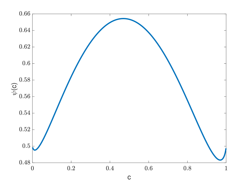
(a) Double-well potential

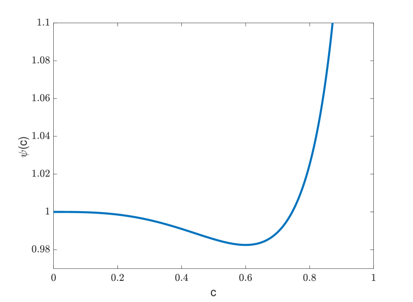
(b) Single-well potential

Figure 7: For both figures $\rho=1$. Double-well logarithmic potential (left) with $\alpha_{1}=1.2$ and $\alpha_{2}=0.8$ and single-well logarithmic potential (right)

To meet the phenomenological observations of the interaction between cells when the mixture is composed of only one cell population (and the other component of the mixture is supposed to be much more compressible), a single-well potential seems more appropriate [15, 19].

Indeed, when the distance between cells falls below a certain value (i.e. if the cell density is large enough), cells are attracted to each other. Then, it exists a threshold value called the mechanical equilibrium for which $\rho H(c_{e})+Q(c_{e})=0$ i.e. there is an equilibrium between attractive and repulsive forces. For larger cell densities, cells are packed too close to each other, they thus experience a repulsive force. When cells are so packed that they fill the whole control volume, then the repulsive force becomes infinite due to the pressure. The representation of such functional is depicted in Figure 7(b). A typical example of single-well potential which has been used for the modeling of living tissue and cancer [19, 7] is

$$\psi_{\text{mix}}(\rho,c)=-(1-c_{e})\log(\rho(1-c))-\frac{c^{3}}{3}-(1-c_{e})\frac{c^{2}}{2}-(1-c_{e})c+k,$$ (B.17)

thus giving

$$H(c)=-(1-c_{e}),\quad Q(c)=-(1-c_{e})\log(1-c)-\frac{c^{3}}{3}-(1-c_{e})\frac{c^{2}}{2}-(1-c_{e})c+k,$$ (B.18)

where $k$ is an arbitrary constant.

References

- [1] H. Abels, On a diffuse interface model for two-phase flows of viscous, incompressible fluids with matched densities, Arch. Ration. Mech. Anal., 194 (2009), pp. 463–506.
- [2] , Strong well-posedness of a diffuse interface model for a viscous, quasi-incompressible two-phase flow, SIAM J. Math. Anal., 44 (2012), pp. 316–340.
- [3] H. Abels, D. Depner, and H. Garcke, On an incompressible Navier-Stokes/Cahn-Hilliard system with degenerate mobility, Ann. Inst. H. Poincaré C Anal. Non Linéaire, 30 (2013), pp. 1175–1190.
- [4] H. Abels and E. Feireisl, On a diffuse interface model for a two-phase flow of compressible viscous fluids, Indiana Univ. Math. J., 57 (2008), pp. 659–698.
- [5] H. Abels, H. Garcke, and G. Grün, Thermodynamically consistent, frame indifferent diffuse interface models for incompressible two-phase flows with different densities, Math. Models Methods Appl. Sci., 22 (2012), pp. 1150013, 40.
- [6] A. Agosti, Discontinuous Galerkin finite element discretization of a degenerate Cahn-Hilliard equation with a single-well potential, Calcolo, 56 (2019), pp. Paper No. 14, 47.
- [7] A. Agosti, P. F. Antonietti, P. Ciarletta, M. Grasselli, and M. Verani, A Cahn-Hilliard-type equation with application to tumor growth dynamics, Math. Methods Appl. Sci., 40 (2017), pp. 7598–7626.
- [8] G. L. Aki, W. Dreyer, J. Giesselmann, and C. Kraus, A quasi-incompressible diffuse interface model with phase transition, Math. Models Methods Appl. Sci., 24 (2014), pp. 827–861.
- [9] D. Ambrosi and L. Preziosi, On the closure of mass balance models for tumor growth, Mathematical Models and Methods in Applied Sciences, 12 (2002), pp. 737–754.
- [10] D. M. Anderson, G. B. McFadden, and A. A. Wheeler, Diffuse-interface methods in fluid mechanics, in Annual review of fluid mechanics, Vol. 30, vol. 30 of Annu. Rev. Fluid Mech., Annual Reviews, Palo Alto, CA, 1998, pp. 139–165.
- [11] J. W. Barrett, J. F. Blowey, and H. Garcke, Finite element approximation of the Cahn-Hilliard equation with degenerate mobility, SIAM J. Numer. Anal., 37 (1999), pp. 286–318.
- [12] D. Bresch and B. Desjardins, Existence of global weak solutions for a 2D viscous shallow water equations and convergence to the quasi-geostrophic model, Comm. Math. Phys., 238 (2003), pp. 211–223.
- [13] , On the construction of approximate solutions for the 2D viscous shallow water model and for compressible Navier-Stokes models, J. Math. Pures Appl. (9), 86 (2006), pp. 362–368.
- [14] D. Bresch, A. F. Vasseur, and C. Yu, Global existence of entropy-weak solutions to the compressible Navier-Stokes equations with non-linear density dependent viscosities, J. Eur. Math. Soc. (JEMS), 24 (2022), pp. 1791–1837.
- [15] H. Byrne and L. Preziosi, Modelling solid tumour growth using the theory of mixtures, Math. Med. Biol., 20 (2003), pp. 341–366.
- [16] J. W. Cahn, On spinodal decomposition, Acta metall., 9 (1961), pp. 795–801.
- [17] J. W. Cahn and J. E. Hilliard, Free Energy of a Nonuniform System. I. Interfacial Free Energy, J. Chem. Phys., 28 (1958), pp. 258–267.
- [18] C. Chatelain, T. Balois, P. Ciarletta, and M. B. Amar, Emergence of microstructural patterns in skin cancer: a phase separation analysis in a binary mixture, New Journal of Physics, 13 (2011), p. 115013.
- [19] C. Chatelain, P. Ciarletta, and M. Ben Amar, Morphological changes in early melanoma development: influence of nutrients, growth inhibitors and cell-adhesion mechanisms, J. Theoret. Biol., 290 (2011), pp. 46–59.
- [20] L. Cherfils, E. Feireisl, M. Michálek, A. Miranville, M. Petcu, and D. Pražák, The compressible Navier-Stokes-Cahn-Hilliard equations with dynamic boundary conditions, Math. Models Methods Appl. Sci., 29 (2019), pp. 2557–2584.
- [21] M. Ebenbeck, H. Garcke, and R. Nürnberg, Cahn–hilliard–brinkman systems for tumour growth, Discrete and Continuous Dynamical Systems - S, 14 (2021), pp. 3989–4033.
- [22] C. Eck, H. Garcke, and P. Knabner, Mathematical modeling, Springer Undergraduate Mathematics Series, Springer, Cham, 2017.
- [23] C. M. Elliott and H. Garcke, On the Cahn-Hilliard equation with degenerate mobility, SIAM J. Math. Anal., 27 (1996), pp. 404–423.
- [24] J. L. Ericksen, Liquid crystals with variable degree of orientation, Arch. Rational Mech. Anal., 113 (1990), pp. 97–120.
- [25] E. Feireisl, Dynamics of viscous compressible fluids, vol. 26 of Oxford Lecture Series in Mathematics and its Applications, Oxford University Press, Oxford, 2004.
- [26] E. Feireisl and A. Novotný, Singular limits in thermodynamics of viscous fluids, Advances in Mathematical Fluid Mechanics, Birkhäuser Verlag, Basel, 2009.
- [27] H. Garcke, K. F. Lam, E. Sitka, and V. Styles, A cahn–hilliard–darcy model for tumour growth with chemotaxis and active transport, Mathematical Models and Methods in Applied Sciences, 26 (2016), pp. 1095–1148.
- [28] J. Giesselmann and T. Pryer, Energy consistent discontinuous Galerkin methods for a quasi-incompressible diffuse two phase flow model, ESAIM Math. Model. Numer. Anal., 49 (2015), pp. 275–301.
- [29] Z. Guo, P. Lin, and J. S. Lowengrub, A numerical method for the quasi-incompressible Cahn-Hilliard-Navier-Stokes equations for variable density flows with a discrete energy law, J. Comput. Phys., 276 (2014), pp. 486–507.
- [30] M. E. Gurtin, On a nonequilibrium thermodynamics of capillarity and phase, Quart. Appl. Math., 47 (1989), pp. 129–145.
- [31] M. E. Gurtin, E. Fried, and L. Anand, The mechanics and thermodynamics of continua, Cambridge University Press, Cambridge, 2010.
- [32] M. E. Gurtin, D. Polignone, and J. Viñals, Two-phase binary fluids and immiscible fluids described by an order parameter, Mathematical Models and Methods in Applied Sciences, 06 (1996), pp. 815–831.
- [33] Q. He and X. Shi, Numerical study of compressible Navier-Stokes-Cahn-Hilliard system, Commun. Math. Sci., 18 (2020), pp. 571–591.
- [34] P. C. Hohenberg and B. I. Halperin, Theory of dynamic critical phenomena, Rev. Mod. Phys., 49 (1977), pp. 435–479.
- [35] B. S. Hosseini, S. Turek, M. Möller, and C. Palmes, Isogeometric analysis of the Navier-Stokes-Cahn-Hilliard equations with application to incompressible two-phase flows, J. Comput. Phys., 348 (2017), pp. 171–194.
- [36] F. Huang and J. Shen, Bound/positivity preserving and energy stable scalar auxiliary variable schemes for dissipative systems: applications to Keller-Segel and Poisson-Nernst-Planck equations, SIAM J. Sci. Comput., 43 (2021), pp. A1832–A1857.
- [37] F. Huang, J. Shen, and K. Wu, Bound/positivity preserving and unconditionally stable schemes for a class of fourth order nonlinear equations, J. Comput. Phys., 460 (2022), pp. Paper No. 111177, 16.
- [38] S. Jin and Z. P. Xin, The relaxation schemes for systems of conservation laws in arbitrary space dimensions, Comm. Pure Appl. Math., 48 (1995), pp. 235–276.
- [39] , The relaxation schemes for systems of conservation laws in arbitrary space dimensions, Comm. Pure Appl. Math., 48 (1995), pp. 235–276.
- [40] K. F. Lam and H. Wu, Thermodynamically consistent Navier-Stokes-Cahn-Hilliard models with mass transfer and chemotaxis, European J. Appl. Math., 29 (2018), pp. 595–644.
- [41] R. J. LeVeque et al., Finite volume methods for hyperbolic problems, vol. 31, Cambridge university press, 2002.
- [42] P.-L. Lions, Mathematical topics in fluid mechanics. Vol. 2, vol. 10 of Oxford Lecture Series in Mathematics and its Applications, The Clarendon Press, Oxford University Press, New York, 1998. Compressible models, Oxford Science Publications.
- [43] , Mathematical topics in fluid mechanics. Vol. 2, vol. 10 of Oxford Lecture Series in Mathematics and its Applications, The Clarendon Press, Oxford University Press, New York, 1998. Compressible models, Oxford Science Publications.
- [44] S. Lisini, D. Matthes, and G. Savaré, Cahn-Hilliard and thin film equations with nonlinear mobility as gradient flows in weighted-Wasserstein metrics, J. Differential Equations, 253 (2012), pp. 814–850.
- [45] I. S. Liu, Method of Lagrange multipliers for exploitation of the entropy principle, Arch. Rational Mech. Anal., 46 (1972), pp. 131–148.
- [46] X. Liu, J. Fang, S. Huang, X. Wu, X. Xie, J. Wang, F. Liu, M. Zhang, Z. Peng, and N. Hu, Tumor-on-a-chip: from bioinspired design to biomedical application, Microsystems & Nanoengineering, 7 (2021), p. 50.
- [47] T. Lorenzi, A. Lorz, and B. Perthame, On interfaces between cell populations with different mobilities, Kinetic and Related Models, 10 (2016), pp. 299–311.
- [48] J. Lowengrub, E. Titi, and K. Zhao, Analysis of a mixture model of tumor growth, European J. Appl. Math., 24 (2013), pp. 691–734.
- [49] , Analysis of a mixture model of tumor growth, European J. Appl. Math., 24 (2013), pp. 691–734.
- [50] J. Lowengrub and L. Truskinovsky, Quasi-incompressible Cahn-Hilliard fluids and topological transitions, R. Soc. Lond. Proc. Ser. A Math. Phys. Eng. Sci., 454 (1998), pp. 2617–2654.
- [51] A. Miranville, The Cahn-Hilliard equation, vol. 95 of CBMS-NSF Regional Conference Series in Applied Mathematics, Society for Industrial and Applied Mathematics (SIAM), Philadelphia, PA, 2019. Recent advances and applications.
- [52] A. Moussa, Some variants of the classical Aubin-Lions lemma, J. Evol. Equ., 16 (2016), pp. 65–93.
- [53] I. Müller, Thermodynamics, Pitman, 1985.
- [54] G. A. Narsilio, O. Buzzi, S. Fityus, T. S. Yun, and D. W. Smith, Upscaling of navier–stokes equations in porous media: Theoretical, numerical and experimental approach, Computers and Geotechnics, 36 (2009), pp. 1200 – 1206.
- [55] B. Perthame and A. Poulain, Relaxation of the Cahn-Hilliard equation with singular single-well potential and degenerate mobility, European J. Appl. Math., 32 (2021), pp. 89–112.
- [56] E. Rocca, G. Schimperna, and A. Signori, On a cahn–hilliard–keller–segel model with generalized logistic source describing tumor growth, Journal of Differential Equations, 343 (2023), pp. 530–578.
- [57] J. Shen, J. Xu, and J. Yang, The scalar auxiliary variable (SAV) approach for gradient flows, J. Comput. Phys., 353 (2018), pp. 407–416.
- [58] , The scalar auxiliary variable (SAV) approach for gradient flows, J. Comput. Phys., 353 (2018), pp. 407–416.
- [59] M. F. P. ten Eikelder, K. G. van der Zee, I. Akkerman, and D. Schillinger, A unified framework for Navier-Stokes Cahn-Hilliard models with non-matching densities, Math. Models Methods Appl. Sci., 33 (2023), pp. 175–221.
- [60] A. F. Vasseur and C. Yu, Existence of global weak solutions for 3D degenerate compressible Navier-Stokes equations, Invent. Math., 206 (2016), pp. 935–974.
- [61] S. M. Wise, J. S. Lowengrub, H. B. Frieboes, and V. Cristini, Three-dimensional multispecies nonlinear tumor growth—I: Model and numerical method, J. Theor. Biol., 253 (2008), pp. 524–543.