Optimal Ball and Horoball Packings Generated by Simply Truncated Coxeter Orthoschemes with Parallel Faces in Hyperbolic $n$-space for $4\leq n\leq 6$

Abstract

After investigating the $3$-dimensional case [35], we continue to address and close the problems of optimal ball and horoball packings in truncated Coxeter orthoschemes with parallel faces that exist in $n$-dimensional hyperbolic space $\overline{\mathbb{H}}^{n}$ up to $n=6$. In this paper, we determine the optimal ball and horoball packing configurations and their densities for the aforementioned tilings in dimensions $4\leq n\leq 6$, where the symmetries of the packings are derived from the considered Coxeter orthoscheme groups. Moreover, for each optimal horoball packing, we determine the parameter related to the corresponding Busemann function, which provides an isometry-invariant description of different optimal horoball packing configurations.

1 Background and preliminaries

According to the known results in $n$-dimensional hyperbolic space $\mathbb{H}^{n}$ ($2\leq n\in\mathbb{N}$), the densest packings of spheres (balls), horospheres (horoballs), and hyperspheres (hyperballs) are achieved through Coxeter simplex tilings. These findings provide a strong motivation for further research on these types of tilings and their associated packings. To begin, let’s review the previous results and background of the topic.

In the realm of discrete geometry, let $X$ represent a space of constant curvature, which can be either the $n$-dimensional sphere $\mathbb{S}^{n}$, Euclidean space $\mathbb{E}^{n}$, or hyperbolic space $\mathbb{H}^{n}$ with $n\geq 2$. One fundamental question in this field is to determine the maximum packing density in $X$ achieved by congruent, non-overlapping balls of a given radius [5], [6]. Defining the packing density in hyperbolic space poses certain challenges, as illustrated by Böröczky’s work [3] and the notable constructions described in references [5] or [29]. To address these challenges, the most widely accepted notion of packing density takes into account the local densities of the balls relative to their Dirichlet-Voronoi cells (see [3] and [12]). In the study of ball and horoball packings in $\overline{\mathbb{H}}^{n}$, we employ an extended concept of such local density.

Let $B$ be a horoball belonging to a packing $\mathcal{B}$, and let $P\in\overline{\mathbb{H}}^{n}$ be an arbitrary point. We define $d(P,B)$ as the shortest distance from point $P$ to the horosphere $S=\partial B$. It should be noted that if $P$ lies within the horoball $B$, then $d(P,B)\leq 0$. The Dirichlet-Voronoi cell $\mathcal{D}(B,\mathcal{B})$ associated with the horoball $B$ can be understood as the convex body or region consisting of all points in $\overline{\mathbb{H}}^{n}$ whose distance to $B$ is smaller than their distance to any other horoball in the packing.

$$\mathcal{D}(B,\mathcal{B})=\{P\in\mathbb{H}^{n}|d(P,B)\leq d(P,B^{\prime}),\leavevmode\nobreak\ \forall B^{\prime}\in\mathcal{B}\}.$$

Both $B$ and $\mathcal{D}$ have infinite volume, therefore the standard notion of local density should be modified. Let $Q\in\partial{\mathbb{H}}^{n}$ denote the ideal center of $B$, and take its boundary $S$ to be the one-point compactification of Euclidean $(n-1)$-space. Let $B_{C}^{n-1}(r)\subset S$ be the Euclidean $(n-1)$-ball with center $C\in S\setminus\{Q\}$. Then $Q$ and $B_{C}^{n-1}(r)$ determine a convex cone $\mathcal{C}^{n}(r)=cone_{Q}\left(B_{C}^{n-1}(r)\right)\in\overline{\mathbb{H}}^{n}$ with apex $Q$ consisting of all hyperbolic geodesics passing through $B_{C}^{n-1}(r)$ with limit point $Q$. The local density $\delta_{n}(B,\mathcal{B})$ of $B$ to $\mathcal{D}$ is defined as

$$\delta_{n}(\mathcal{B},B)=\varlimsup\limits_{r\rightarrow\infty}\frac{\mathrm{vol}(B\cap\mathcal{C}^{n}(r))}{\mathrm{vol}(\mathcal{D}\cap\mathcal{C}^{n}(r))}.$$

This limit is independent of the choice of center $C$ for $B^{n-1}_{C}(r)$.

In the case of periodic ball or horoball packings, this local density defined above extends to the entire hyperbolic space via its symmetry group, and is related to the simplicial density function (defined below) that we generalized in [33] and [34]. In this paper, we shall use such definition of packing density.

A Coxeter simplex is a top dimensional simplex in $X$ with dihedral angles either integral submultiples of $\pi$ or $0$. The group generated by reflections on the sides of a Coxeter simplex is a Coxeter simplex reflection group. Such reflections generate a discrete group of isometries of $X$ with the Coxeter simplex as the fundamental domain; hence the groups give regular tessellations of $X$, if the fundamental simplex is characteristic. The Coxeter groups are finite for $\mathbb{S}^{n}$, and infinite for $\mathbb{E}^{n}$ or $\overline{\mathbb{H}}^{n}$. There are non-compact Coxeter simplices in $\overline{\mathbb{H}}^{n}$ with ideal vertices on $\partial\mathbb{H}^{n}$, however only for dimensions $2\leq n\leq 9$; furthermore, only a finite number exists in dimensions $n\geq 3$. Johnson et al. [11] found the volumes of all Coxeter simplices in hyperbolic $n$-space. Such simplices are the most elementary building blocks of hyperbolic manifolds, the volume of which is an important topological invariant. Of course, if we allow the simplexes to have “outer” vertices, the number of possible simplexes expands and we get nice new tilings (see e.g. [8, 9]). Our work is also related to one of these classes.

In $n$-dimensional space $X$ of constant curvature $(n\geq 2)$, define the simplicial density function $d_{n}(r)$ to be the density of $n+1$ mutually tangent balls of radius $r$ in the simplex spanned by their centers. L. Fejes Tóth and H. S. M. Coxeter conjectured that the packing density of balls of radius $r$ in $X$ cannot exceed $d_{n}(r)$. Rogers [30] proved this conjecture in Euclidean space $\mathbb{E}^{n}$. The $2$-dimensional spherical case was settled by L. Fejes Tóth [7], and Böröczky [3] gave a proof for the extension. In hyperbolic 3-space, the monotonicity of $d_{3}(r)$ was proved by Böröczky and Florian in [4]; in [23] Marshall showed that for sufficiently large $n$, function $d_{n}(r)$ is strictly increasing in variable $r$. Kellerhals [12] showed $d_{n}(r)<d_{n-1}(r)$, and that in cases considered by Marshall the local density of each ball in its Dirichlet–Voronoi cell is bounded above by the simplicial horoball density $d_{n}(\infty)$.

The simplicial ball and horoball packing density upper bound $d_{3}(\infty)=(1+\frac{1}{2^{2}}-\frac{1}{4^{2}}-\frac{1}{5^{2}}+\frac{1}{7^{2}}+\frac{1}{8^{2}}-\frac{1}{10^{2}}-\frac{1}{11^{2}}+\dots)^{-1}=0.85327\dots$ cannot be achieved by packing regular balls, instead, it is realized by horoball packings of $\overline{\mathbb{H}}^{3}$, the regular ideal simplex tiles $\overline{\mathbb{H}}^{3}$. More precisely, the centers of horoballs in $\partial\overline{\mathbb{H}}^{3}$ lie at the vertices of the ideal regular Coxeter simplex tiling with Schläfli symbol $\{3,3,6\}$.

In three dimensions, the Böröczky-type bound for horoball packings are used for volume estimates of cusped hyperbolic manifolds [1, 25], more recently [2, 24]. Lifts of horoball neighborhoods of cusps give horoball packings in the universal cover $\mathbb{H}^{n}$, and for some discrete torsion-free subgroup of isometries $\mathbb{H}^{n}/\Gamma$ is a cusped hyperbolic manifold where the cusps lift to ideal vertices of the fundamental domain. In this setting, a manifold with a single cusp has a well-defined maximal cusp neighborhood, while manifolds with multiple cusps have a range of non-overlapping cusp neighborhoods with boundaries with nonempty tangential intersection, these lift to different horoball types in the universal cover. An important application is Adams’ proof that the Geiseking manifold is the noncompact hyperbolic $3$-manifold of minimal volume [1] (further information [28]). Kellerhals then used the Böröczky-type bounds to estimate volumes of higher dimensional hyperbolic manifolds [13].

In [18], we proved that the classical horoball packing configuration in $\overline{\mathbb{H}}^{3}$ realizing the Böröczky-type upper bound is not unique. We gave several examples of different regular horoball packings using horoballs of different types, that is horoballs that have different relative densities with respect to the fundamental domain, that yield the Böröczky–Florian-type simplicial upper bound [4].

Furthermore, in [33, 34] we found that by allowing horoballs of different types at each vertex of a totally asymptotic simplex and generalizing the simplicial density function to $\overline{\mathbb{H}}^{n}$ for $n\geq 2$, the Böröczky-type density upper bound is not valid for the fully asymptotic simplices for $n\geq 4$. In $\overline{\mathbb{H}}^{4}$, the locally optimal simplicial packing density is $0.77038\dots$, higher than the Böröczky-type density upper bound of $d_{4}(\infty)=0.73046\dots$ using horoballs of a single type. However, these ball packing configurations are only locally optimal and cannot be extended to the entirety of $\overline{\mathbb{H}}^{n}$. Further interesting constructions are described in [31, 32].

In a series of $5$ papers, the optimal horoball packing configurations and their densities of Koszul-type noncompact Coxeter simplex tilings were investigated by R. T. Kozma and the second author where these tilings exist in $\overline{\mathbb{H}}^{n}$ for $2\leq n\leq 9$ (see [18, 19, 20, 21]). In [22], we studied some further new aspects of the topic.

We would highlight only one of them here, in [19], we found seven horoball packings of Coxeter simplex tilings in $\overline{\mathbb{H}}^{4}$ that yield densities of $5\sqrt{2}/\pi^{2}\approx 0.71645$, counterexamples to L. Fejes Tóth’s conjecture for the maximal packing density of $\frac{5-\sqrt{5}}{4}\approx 0.69098$ in his foundational book Regular Figures [7, p. 323]. We note here, that this density is realized also in our case with Schläfli symbol $\{4,4,3,4,\infty\}$ (see Theorem 4.4).

In Table 1, we summarize the Böröczky-type upper bound densities $d_{n}(\infty)$ (see [12]) and the densities of the densest known horoball arrangements which we found in our previous papers.

$n$	Optimal Coxeter simplex packing density	Numerical Value	$d_{n}(\infty)$	$\Delta$
3	$\left(1+\frac{1}{2^{2}}-\frac{1}{4^{2}}-\frac{1}{5^{2}}+\frac{1}{7^{2}}+\frac{1}{8^{2}}-\dots\right)^{-1}$	0.85328…	0.85328…	0
4	$5\sqrt{2}/\pi^{2}$	0.71644…	0.73046…	0.0140…
5	$\displaystyle 5/\left(7\zeta(3)\right)$	0.59421…	0.60695…	0.0127…
6	$81/\left(4\sqrt{2}\pi^{3}\right)$	0.46180…	0.49339…	0.0315…
7	$\displaystyle 28/\left(81\text{L}(4,3)\right)$	0.36773…	0.39441…	0.0266…
8	$\displaystyle 225/\left(8\pi^{4}\right)$	0.288731…	0.31114…	0.0223…
9	$1/\left(4\zeta(5)\right)$	0.24109…	0.24285…	0.0017…

Table 1: Packing density upper and lower bounds for $\overline{\mathbb{H}}^{n}$, where $\zeta(\cdot)$ is the Riemann Zeta function, $\text{L}(\cdot,\cdot)$ is the Dirichlet $L$-Series and $\Delta$ is the gap between the packing density upper bound and our effective lower bounds.

In [35], we considered the ball and horoball packings belonging to $3$-dimensional Coxeter tilings that are derived by simply truncated orthoschemes with parallel faces. We determined the optimal ball and horoball packing arrangements and their densities for all above Coxeter tilings in hyperbolic $3$-space $\mathbb{H}^{3}$. The centers of horoballs are required to lie at ideal vertices of the polyhedral cells constituting the tiling, and we allow horoballs of different types at the various vertices (using Busemann function parametrization of horoballs). We proved that the densest packings are realized by horoballs related to tiling $\{\infty,3,6,\infty\}$ and to its dual $\{\infty,6,3,\infty\}$ with density $\approx 0.8413392$.

In this paper, we continue and close the problem of optimal ball and horoball packings related to truncated Coxeter orthoschemes with parallel faces that exist in $n$-dimensional hyperbolic space $\overline{\mathbb{H}}^{n}$ up to $n=6$, determine the optimal ball and horoball packing configurations and their densities of the above tilings in dimensions $4\leq n\leq 6$. We prove, that the optimal ball and horoball densities coincide with the known density lower bounds (see Table 1) in $4$- and $5$ dimensions and less in $6$-dimension. Particularly in $\overline{\mathbb{H}}^{4}$, it is attained by two horoballs related to $\{4,4,3,4,\infty\}$ tiling with density $\frac{5\sqrt{2}}{\pi^{2}}\approx 0.71645$. In $\overline{\mathbb{H}}^{5}$, $\frac{5}{7\zeta{3}}\approx 0.59421$, realized by horoballs related to $\{4,3,4,3,3,\infty\}$ Coxeter orthoscheme tiling. While in $\overline{\mathbb{H}}^{6}$, we have optimum value $\frac{15\sqrt{2}+18}{4\pi^{3}}\approx 0.31617$, reached by horoball packing related to Coxeter tiling $\{3,4,3,3,3,4,\infty\}$.

Our method for computing densities in the projective Beltrami–Cayley–Klein model is mostly similar to the earlier $3$-dimensional case (see [35, 36]), although the computations are much more complicated and require new methods, especially in volume calculations.

2 Basic Notions

2.1 The projective model of hyperbolic space $\mathbb{H}^{n}$

Let $\mathbb{E}^{1,n}$ denote $\mathbb{R}^{n+1}$ with the Lorentzian inner product $\langle\mathbf{x},\mathbf{y}\rangle=-x^{0}y^{0}+x^{1}y^{1}+\dots+x^{n}y^{n}$ where non-zero real vectors $\mathbf{x,y}\in\mathbb{R}^{n+1}$ represent points in projective space $\mathbb{P}^{n}=\mathbb{P}(\mathbb{E}^{n+1})$, equipped with the quotient topology of the natural projection $\Pi:\mathbb{E}^{n+1}\setminus\{\mathbf{0}\}\rightarrow\mathbb{P}^{n}$. Partitioning $\mathbb{E}^{1,n}$ into $Q_{+}=\{\mathbf{v}\in\mathbb{R}^{n+1}|\langle\mathbf{v},\mathbf{v}\rangle>0\}$, $Q_{0}=\{\mathbf{v}|\langle\mathbf{v},\mathbf{v}\rangle=0\}$, and $Q_{-}=\{\mathbf{v}|\langle\mathbf{v},\mathbf{v}\rangle<0\}$, the proper points of hyperbolic $n$-space are $\mathbb{H}^{n}=\Pi(Q_{-})$, $\partial\mathbb{H}^{n}=\Pi(Q_{0})$ are the boundary or ideal points, we will refer to points in $\Pi(Q_{+})$ as outer points, and $\overline{\mathbb{H}}^{n}=\mathbb{H}^{n}\cup\partial\mathbb{H}^{n}$ as extended hyperbolic space.

Points $[\mathbf{x}],[\mathbf{y}]\in\mathbb{P}^{n}$ are conjugate when $\langle\mathbf{x},\mathbf{y}\rangle=0$. The set of all points conjugate to $[\mathbf{x}]$ form a projective (polar) hyperplane $Pol([\mathbf{x}])=\{[\mathbf{y}]\in\mathbb{P}^{n}|\langle\mathbf{x},\mathbf{y}\rangle=0\}.$ Hence $Q_{0}$ induces a duality $\mathbb{R}^{n+1}\leftrightarrow\mathbb{R}_{n+1}$ between the points and hyperplanes of $\mathbb{P}^{n}$. Point $[\mathbf{x}]$ and hyperplane $[\boldsymbol{a}]$ are incident if the value of the linear form $\boldsymbol{a}$ evaluated on vector $\mathbf{x}$ is zero, i.e. $\mathbf{x}\boldsymbol{a}=0=\langle\mathbf{x},\mathbf{a}\rangle$ where $\mathbf{x}\in\ \mathbb{R}^{n+1}\setminus\{\mathbf{0}\}$, and $\boldsymbol{a}\in\mathbb{R}_{n+1}\setminus\{\mathbf{0}\}$. Similarly, the lines in $\mathbb{P}^{n}$ are given by 2-subspaces of $\mathbb{R}^{n+1}$ or dual $(n-1)$-subspaces of $\mathbb{R}_{n+1}$ [26].

In this paper, we set the sectional curvature of $\mathbb{H}^{n}$, $K=-k^{2}$, to be $k=1$. The distance $d$ between two proper points $[\mathbf{x}]$ and $[\mathbf{y}]$ is given by

$$\cosh{{d}}=\frac{-\langle\mathbf{x},\mathbf{y}\rangle}{\sqrt{\langle\mathbf{x},\mathbf{x}\rangle\langle\mathbf{y},\mathbf{y}\rangle}}.$$ (2.1)

The projection $[\mathbf{y}]$ of point $[\mathbf{x}]$ on plane $[\mathbf{u}]$ is given by

$$\mathbf{y}=\mathbf{x}-\frac{\langle\mathbf{x},\mathbf{u}\rangle}{\langle\boldsymbol{u},\boldsymbol{u}\rangle}\mathbf{u},$$ (2.2)

where $[\mathbf{u}]$ is the pole of the hypeplane $[\boldsymbol{u}]$.

2.2 On Horoballs

A horosphere in $\overline{\mathbb{H}}^{n}$ ($n\geq 2)$ is as hyperbolic $n$-sphere with infinite radius centered at an ideal point $\xi\in\partial\mathbb{H}^{n}$ obtained as a limit of spheres through $x\in\mathbb{H}^{n}$ as its center $c\rightarrow\xi$. Equivalently, a horosphere is an $(n-1)$-surface orthogonal to the set of parallel straight lines passing through $\xi\in\partial\mathbb{H}^{n}$. A horoball is a horosphere together with its interior.

To derive the equation of a horosphere, we fix a projective coordinate system for $\mathbb{P}^{n}$ with standard basis $\mathbb{a}_{i},0\leq i\leq n$ so that the Cayley–Klein ball model of $\overline{\mathbb{H}}^{n}$ is centered at $O=(1,0,0,\dots,0)$, and orient it by setting point $\xi\in\partial\mathbb{H}^{n}$ to lie at $A_{0}=(1,0,\dots,0,1)$. The equation of a horosphere with center $\xi=A_{0}$ passing through interior point $S=(1,0,\dots,0,s)$ is derived from the equation of the the boundary sphere $-x^{0}x^{0}+x^{1}x^{1}+x^{2}x^{2}+\dots+x^{n}x^{n}=0$, and the plane $x^{0}-x^{n}=0$ tangent to the boundary sphere at $\xi=A_{0}$. The general equation of the horosphere is

$$0=\lambda(-x^{0}x^{0}+x^{1}x^{1}+x^{2}x^{2}+\dots+x^{n}x^{n})+\mu{(x^{0}-x^{n})}^{2}.$$ (2.3)

Evaluating at $S$ obtain

$$\lambda(-1+s^{2})+\mu{(-1+s)}^{2}=0\text{\leavevmode\nobreak\ \leavevmode\nobreak\ and\leavevmode\nobreak\ \leavevmode\nobreak\ }\frac{\lambda}{\mu}=\frac{1-s}{1+s}.$$

For $s\neq\pm 1$, the equation of a horosphere in projective coordinates is

$$(s-1)\left(-x^{0}x^{0}+\sum_{i=1}^{n}(x^{i})^{2}\right)-(1+s){(x^{0}-x^{n})}^{2} =0.$$ (2.4)

Remark 2.1

The last form can be considered in the spherical coordinate parameterization (It is powerful to provide a horosphere visualization.)

$$h_{1}=\sqrt{\frac{1-s}{2}}\sin{\theta_{1}}\sin{\theta_{2}}\cdots\sin{\theta_{n-1}}$$

$$h_{2}=\sqrt{\frac{1-s}{2}}\sin{\theta_{1}}\sin{\theta_{2}}\cdots\cos{\theta_{n-1}}$$

$$\vdots\hskip 56.9055pt\vdots$$

$$h_{n-1}=\sqrt{\frac{1-s}{2}}\sin{\theta_{1}}\cos{\theta_{2}}$$

$$h_{n}=\frac{1+s}{2}+\frac{1-s}{2}\cos{\theta_{1}},$$

where $0\leq\theta_{i}\leq\pi,i\in\{1\dots n-2\}$ and $0\leq\theta_{n-1}<2\pi$.

In $\overline{\mathbb{H}}^{n}$, there exists an isometry $g\in\text{Isom}(\mathbb{H}^{n})$ for any two horoballs $B$ and $B^{\prime}$ such that $g.B=B^{\prime}$. However, it is often useful to distinguish between certain horoballs of a packing; we shall use the notion of horoball type with respect to the fundamental domain of a tiling (lattice) as introduced in [34]. In [21], we showed that this coincides with the Busemann function up to scaling, hence is isometry invariant.

Two horoballs of a horoball packing are said to be of the same type or equipacked if and only if their local packing densities with respect to a particular cell (in our case a Coxeter simplex) are equal, otherwise, the two horoballs are of different type. For example, the horoballs centered at $A_{0}$ passing through $S$ with different values for the final coordinate $s\in(-1,1)$ are of different type relative to a given cell and the set of all horoballs centered at vertex $A_{0}$ is a one-parameter family.

Volumes of horoball pieces are given by János Bolyai’s classical formulas. The hyperbolic length $L(x)$ of a horospherical arc corresponded to a chord segment of length $x$ is

$$L(x)=2\sinh{\left(\tfrac{x}{2}\right)}.$$ (2.5)

As the intrinsic geometry of a horosphere is Euclidean, the $(n-1)$-dimensional volume $\mathrm{vol}\mathcal{A}$ of a polyhedron $\mathcal{A}$ on the surface of the horosphere can be calculated as in $\mathbb{E}^{n-1}$. The volume of the horoball piece $\mathcal{H}(\mathcal{A})$ bounded by $\mathcal{A}$, and the set of geodesic segments joining $\mathcal{A}$ to the center of the horoball, is

$$\mathrm{vol}(\mathcal{H}(\mathcal{A}))=\tfrac{1}{n-1}\mathrm{vol}\mathcal{A}.$$ (2.6)

2.3 Coxeter orthoschemes and tilings

In the $\overline{\mathbb{H}}^{n}$ $(2\leq n\in\mathbb{N})$ space, a complete orthoscheme $\mathcal{S}$ of degree $d$ $(0\leq d\leq 2)$ is a polytope bounded with hyperplanes $H^{0},...,H^{n+d}$, for which $H^{i}\perp H^{j}$, if $j\neq i-1,i,i+1$. We denote $A_{i}$ as the vertex opposite to the hyperplane $H^{i}$ where ($0\leq i\leq n$). Equivalently, the orthoscheme can be described by the sequence of the vertices of the orthoschemes $A_{0},...,A_{n}$, where $A_{i-1}A_{i}$ edge is perpendicular to $A_{i}A_{i+1}$ edge for all $i\in\{1,...,n-1\}$. Here, $A_{0}$ and $A_{n}$ are called the principal vertices of the orthoschemes.

Now, consider the reflections on the facets of the simply truncated orthoscheme $H^{1},\cdot,H^{n+1}$, and denote them with $r_{0},...,r_{n+1}$, hence define the group

$$\mathbf{G}=\langle r_{0},...,r_{n+1}|(r_{i}r_{j})^{m_{ij}}=1\rangle,$$

where $\alpha^{ij}=\frac{\pi}{m_{ij}}$, and $m_{ii}=1$. Note that, if $m_{ij}=\infty$ (i.e. $H^{i}$ and $H^{j}$ are parallel), then the $r_{i},r_{j}$ pair belongs to no relation. Here, $2\leq m_{ij}\in\{\mathbb{N}\cup\infty\}$, $i\neq j$. Since the Coxeter group $\mathbf{G}$ acts on hyperbolic space $\overline{\mathbb{H}}^{n}$ properly discontinuously, then the images of the orthoscheme under this action provide a $\mathcal{T}$ tiling of $\overline{\mathbb{H}}^{n}$ i.e. the images of the orthoscheme fills $\overline{\mathbb{H}}^{n}$ without overlap.

Let $S\subset\overline{\mathbb{H}}^{n}$ denote a complete orthoscheme bounded by a finite set of hyperplanes $H^{i}$ with unit normal forms $\mbox{\boldmath$b$}^{i}\in\mbox{\boldmath$V$}\!_{n+1}$ directed outwards the interior of $S$:

$$H^{i}:=\{\mathbf{x}\in\mathbb{H}^{n}|\mathbf{x}\leavevmode\nobreak\ \mbox{\boldmath$b$}^{i}=0\}\ \ \text{with}\ \ \langle\mbox{\boldmath$b$}^{i},\mbox{\boldmath$b$}^{i}\rangle=1.$$ (2.7)

The Grammian matrix $G(\mathcal{S}):=(\langle\mbox{\boldmath$b$}^{i},\mbox{\boldmath$b$}^{j}\rangle)_{i,j}\leavevmode\nobreak\ {i,j\in\{0,1,2\dots n\}}$ is an indecomposable symmetric matrix of signature $(1,n)$ with entries $\langle\mbox{\boldmath$b$}^{i},\mbox{\boldmath$b$}^{i}\rangle=1$ and $\langle\mbox{\boldmath$b$}^{i},\mbox{\boldmath$b$}^{j}\rangle\leq 0$ for $i\neq j$ where

$$\langle\mbox{\boldmath$b$}^{i},\mbox{\boldmath$b$}^{j}\rangle=\left\{\begin{aligned} &0&&\text{if}\leavevmode\nobreak\ H^{i}\perp H^{j},\\ &-\cos{\alpha^{ij}}&&\text{if}\leavevmode\nobreak\ H^{i},H^{j}\leavevmode\nobreak\ \text{intersect \ along an edge of $P$ \ at \ angle}\ \alpha^{ij},\\ &-1&&\text{if}\leavevmode\nobreak\ \ H^{i},H^{j}\leavevmode\nobreak\ \text{are parallel in the hyperbolic sense},\\ &-\cosh{l^{ij}}&&\text{if}\leavevmode\nobreak\ H^{i},H^{j}\leavevmode\nobreak\ \text{admit a common perpendicular of length}\ l^{ij}.\end{aligned}\right.$$

For the complete Coxeter orthoschemes $\mathcal{S}\subset\overline{\mathbb{H}}^{n}$, we adopt the conventions for the Coxeter graph: if the dihedral angle between two hyperplane faces is $\frac{\pi}{m_{ij}}$, then two related nodes are joined by an edge of weight $m_{ij}$. If the two hyperplane faces are orthogonal then the two corresponding nodes are disjoint. In the hyperbolic case if two bounding hyperplanes of $S$ are parallel, then the corresponding nodes are joined by a line marked $\infty$. If they are divergent then their nodes are joined by a dotted line.

In general, the Coxeter orthoschemes were classified by H-C. Im Hof in [8] and [9] where he proved that they exist in dimension $\leq 9$, and gave a full list.

In this paper we consider a class of simply truncated orthoschemes where $d=1$. That means, that one of its principal vertices (e.g. $A_{n-1}$) is the outer point related to the projective model, so they are truncated by its polar hyperplane $Pol(A_{n-1})$. Moreover, we assume that $Pol(A_{n-1})$ and the hyperplane $H_{0}$ are parallel. We obtain the above classification of the Coxeter orthoschemes that such tilings exist only in $3,4,5$ and $6$-dimensional hyperbolic spaces $\overline{\mathbb{H}}^{n}$.

Packing problems related to the three-dimensional case were investigated in papers [35], [36] thus in the following we concentrate on $\overline{\mathbb{H}}^{n}$ with dimensions $n=4,5,6$. We note here that with these analyses, we close the examination of these tiling types and the corresponding packing problems.

We begin by recalling the list of Coxeter graphs that give truncated orthoscheme with parallel faces (see Fig.1–3), and describing their Coxeter graph for $n=4,5,6$.

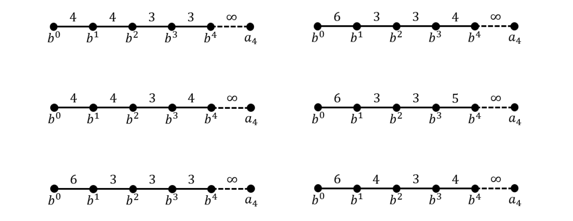
Figure 1: Coxeter graph of simply truncated orthoschemes with parallel faces in $\overline{\mathbb{H}}^{4}$

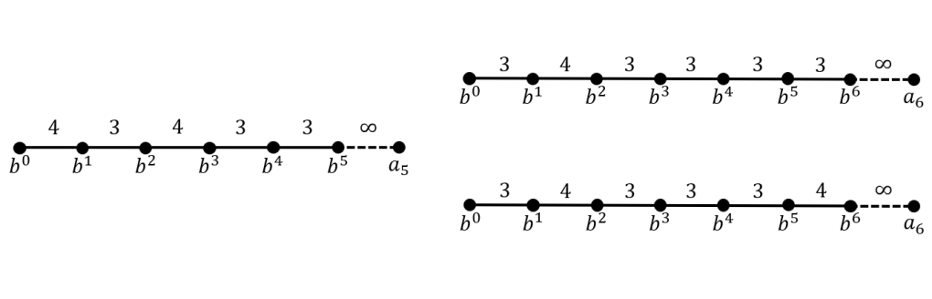
Figure 2: Coxeter graph of simply truncated orthoschemes with parallel faces in $\overline{\mathbb{H}}^{5}$ (left) and in $\overline{\mathbb{H}}^{6}$ (right)

We have obtained $6$ types of Coxeter tilings in $\overline{\mathbb{H}}^{4}$, $1$ type and $2$ types for $\overline{\mathbb{H}}^{5}$ and $\overline{\mathbb{H}}^{6}$ respectively. The structures of truncated orthoschemes (the fundamental domains of the considered tilings) in $\overline{\mathbb{H}}^{4}$ and $\overline{\mathbb{H}}^{5}$ are illustrated in Fig. 4.

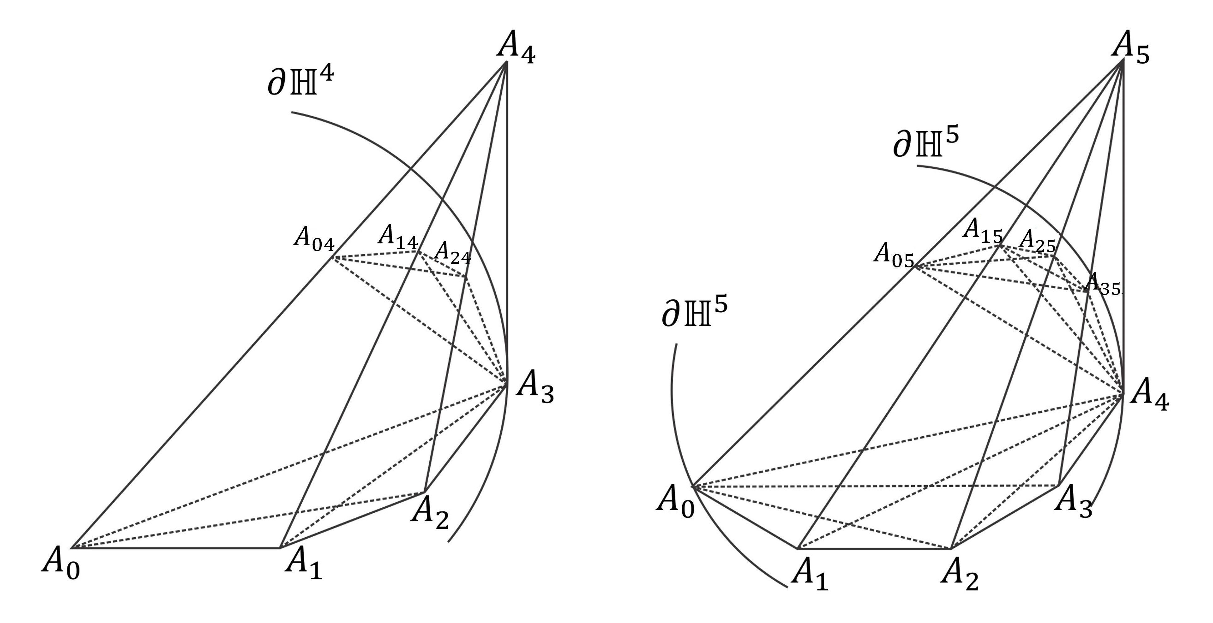
Figure 3: The structure of a truncated orthoscheme in $\overline{\mathbb{H}}^{4}$, the vertex $A_{3}$ is an ideal, $A_{4}$ is ultra-ideal, while $A_{0}$ is either proper or ideal. The polar hyperplane of $A_{4}$ is given by $A_{3}A_{04}A_{14}A_{24}$ (left). The truncated orthoscheme in $\overline{\mathbb{H}}^{5}$, the vertex $A_{4}$ is an ideal, $A_{5}$ is ultra-ideal, while $A_{0}$ is either proper or ideal. The polar hyperplane of $A_{5}$ is represented by points $A_{4}A_{05}A_{15}A_{25}A_{35}$ (right)

Therefore, we shall consider the classical ball and horoball packings related to truncated orthoschemes with these Schläfli symbols. We shall apply the methods used in $3$-dimensional cases ([35, 36] with some important generalizations to higher dimensions.

2.3.1 The volumes of orthoschemes in even dimensions

The area formula for planar orthoschemes, which are right-angled triangles, is widely known as the defect formula. L. Schläfli extended this formula to spherical orthoschemes of even dimensions. Schläfli’s reduction formula expresses the volume of an even-dimensional spherical orthoscheme in terms of the volumes of certain lower-dimensional orthoschemes. This formula can be straightforwardly extended to the hyperbolic case through analytic continuation.

In [14], R. Kellerhals further extended this formula to a specific class of hyperbolic polytopes called (complete) orthoschemes of degree $d$ (where $d\in{0,1,2}$). These polytopes arise in the study of hyperbolic Coxeter groups and are a particular type of fundamental polytope. R. Kellerhals demonstrated that the generalized reduction formula holds for even-dimensional complete orthoschemes and determined their volumes for all possible complete orthoschemes in dimensions $n$, where $n\in{4,6,8}$.

In Table 2, we recall the volumes obtained for the even-dimensional orthoschemes we examined.

[.5]() Dimension	Schläfli symbol	$\mathrm{vol}(\widehat{\mathcal{S}})$.
[.5]() 4	$\{4,4,3,3,\infty\}$	$\frac{\pi^{2}}{288}\approx 0.03427$
[.5]() 4	$\{4,4,3,4,\infty\}$	$\frac{\pi^{2}}{144}\approx 0.06854$
[.5]() 4	$\{6,3,3,3,\infty\}$	$\frac{\pi^{2}}{540}\approx 0.01828$
[.5]() 4	$\{6,3,3,4,\infty\}$	$\frac{\pi^{2}}{288}\approx 0.03427$
[.5]() 4	$\{6,3,3,5,\infty\}$	$\frac{61\pi^{2}}{900}\approx 0.66894$
[.5]() 4	$\{6,3,4,3,\infty\}$	$\frac{5\pi^{2}}{864}\approx 0.05712$
[.5]() 6	$\{3,4,3,3,3,3,\infty\}$	$\frac{11\pi^{3}}{86,400}\approx 0.00395$
[.5]() 6	$\{3,4,3,3,3,4,\infty\}$	$\frac{\pi^{3}}{86,400}\approx 0.00036$

Table 2: Volumes of truncated orthoschemes with parallel faces in $\overline{\mathbb{H}}^{4}$ and $\overline{\mathbb{H}}^{6}$.

2.3.2 Volumes of orthoschemes in $\overline{\mathbb{H}}^{5}$

In contrast to the cases of $\overline{\mathbb{H}}^{4}$ and $\overline{\mathbb{H}}^{6}$, the volumes of simply truncated orthoschemes in $\overline{\mathbb{H}}^{5}$ cannot be expressed by a simple closed formula. To overcome this challenge, we employ a method known as the scissor congruence method, which involves decomposing the orthoscheme into several smaller orthoschemes (see [15]). These smaller orthoschemes must satisfy the condition of being double asymptotic orthoschemes, allowing their volumes to be computed using a formula established by R. Kellerhals in [16, 17]. This formula utilizes the ellipticity and parabolicity conditions of the principal vertices, specifically $A_{0}$ and $A_{5}$, within the orthoscheme $\mathcal{S}$.
Consider an orthoscheme $\mathcal{S}$ with a Coxeter-Schläfli matrix denoted as $(b^{ij})$, and let ${v_{1},v_{2},v_{3},v_{4},v_{5}}$ represent its Schläfli symbol. Within this context, $(b^{ij})_{0}$ and $(b^{ij})_{5}$ refer to the principal submatrices of $(b^{ij})$ obtained by removing the corresponding rows and columns associated with the vertices $A_{0}$ and $A_{5}$ respectively. Geometrically, this removal process corresponds to eliminating the opposite face of the vertex $A_{0}$ or $A_{5}$ from the orthoscheme $\mathcal{S}$, resulting in a simplicial cone structure.

We have the following elliptic/parabolic conditions:

1. If $(b^{ij})_{0}$ and $(b^{ij})_{5}$ are positive definite, then $A_{0}$ and $A_{5}$ are a proper vertices and it said to be elliptic.

2. If $(b^{ij})_{0}$ and $(b^{ij})_{5}$ are positive semi-definite, then $A_{0}$ and $A_{5}$ are ideal vertices and it said to be parabolic.

Through the analysis of the corresponding polynomials associated with these submatrices, the following findings emerge:

1. $(b^{ij})_{0}$, and $(b^{ij})_{5}$ are positive definite,
   $\displaystyle\frac{\cos^{2}{\left(\frac{\pi}{v_{3}}\right)}}{\sin^{2}{\left(\frac{\pi}{v_{2}}\right)}}+\frac{\cos^{2}{\left(\frac{\pi}{v_{4}}\right)}}{\sin^{2}{\left(\frac{\pi}{v_{5}}\right)}}<1$,   $\displaystyle\frac{\cos^{2}{\left(\frac{\pi}{v_{2}}\right)}}{\sin^{2}{\left(\frac{\pi}{v_{1}}\right)}}+\frac{\cos^{2}{\left(\frac{\pi}{v_{3}}\right)}}{\sin^{2}{\left(\frac{\pi}{v_{4}}\right)}}<1$.

2. $(b^{ij})_{0}$ and $(b^{ij})_{5}$ are semi-positive definite,
   $\displaystyle\frac{\cos^{2}{\left(\frac{\pi}{v_{3}}\right)}}{\sin^{2}{\left(\frac{\pi}{v_{2}}\right)}}+\frac{\cos^{2}{\left(\frac{\pi}{v_{4}}\right)}}{\sin^{2}{\left(\frac{\pi}{v_{5}}\right)}}=1$,   $\displaystyle\frac{\cos^{2}{\left(\frac{\pi}{v_{2}}\right)}}{\sin^{2}{\left(\frac{\pi}{v_{1}}\right)}}+\frac{\cos^{2}{\left(\frac{\pi}{v_{3}}\right)}}{\sin^{2}{\left(\frac{\pi}{v_{4}}\right)}}=1$.

By employing the scissor congruence method, we can decompose the simply truncated $\widehat{\mathcal{S}}$ orthoscheme with the Schläfli symbol $\{4,3,4,3,3,\infty\}$ into several smaller orthoschemes.
The polar hyperplane $Pol(A_{5})$ of the ultra-ideal vertex $A_{5}$ encompasses the ideal vertex $A_{4}$ of $\mathcal{S}$. The intersections of $Pol(A_{5})$ with the edges $A_{i}A_{5}$ (where $i\in\{0,1,2,3\}$) are denoted as $A_{i5}$. For a visual representation, please refer to Figure 3. The truncated orthoscheme $\widehat{\mathcal{S}}$ can be dissected into some “smaller” doubly asymptotic orthoschemes $R_{j}$, $(j\in\{1,\dots 4\})$ where each of them is the convex hull of vertices:

$$R_{1}:=conv(A_{0},A_{05},A_{15},A_{25},A_{35},A_{4})\leavevmode\nobreak\ \leavevmode\nobreak\ \leavevmode\nobreak\ R_{2}:=conv(A_{0},A_{1},A_{15},A_{25},A_{35},A_{4})$$

$$R_{3}:=conv(A_{0},A_{1},A_{2},A_{25},A_{35},A_{4})\leavevmode\nobreak\ \leavevmode\nobreak\ \leavevmode\nobreak\ \leavevmode\nobreak\ R_{4}:=conv(A_{0},A_{1},A_{2},A_{3},A_{35},A_{4}).$$

Therefore, the volume of $\widehat{\mathcal{S}}$ can be computed as

$$\mathrm{vol}(\widehat{\mathcal{S}})=\sum_{i=1}^{4}\mathrm{vol}(R_{i}).$$

By following the method described by Kellerhals in [15], the dihedral angles of orthoschemes $R_{1},R_{2},R_{3}$, and $R_{4}$ can be computed by the following method using their Coxeter graphs, (see Fig. 4).

Based on the structure of $\widehat{\mathcal{S}}$, we can derive the following two equations directly:

$$\frac{\pi}{p_{1}}+\frac{\pi}{p_{2}}=\frac{\pi}{2},\leavevmode\nobreak\ \leavevmode\nobreak\ \frac{\pi}{s_{1}}+\frac{\pi}{s_{2}}=\frac{\pi}{2}.$$

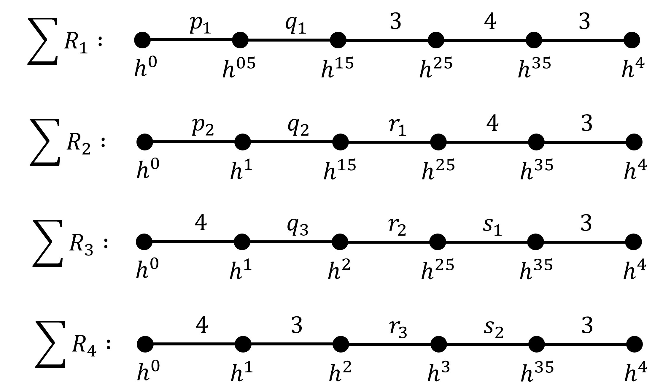
Figure 4: Coxeter graph of dissected doubly asymptotic orthoschemes $R_{j}$, $(j\in\{1,2,3,4\})$. Here, $h^{k}$ denotes the opposite face of vertex $A_{k}$ in each corresponding $R_{j}$

The first equation arises from the consideration of the angles $\frac{\pi}{p_{1}}$ and $\frac{\pi}{p_{2}}$ associated with the vertices $A_{15},A_{25},A_{35},A_{4}$ in 3-space. These angles are present in the shared portion of the hyperplane faces $A_{05}A_{15}A_{25}A_{35}A_{4}$, $A_{0}A_{15}A_{25}A_{35}A_{4}$, and $A_{1}A_{15}A_{25}A_{35}A_{4}$. The second equation results from the presence of the angles $\frac{\pi}{s_{1}}$ and $\frac{\pi}{s_{2}}$ on the edge $A_{2}A_{4}$, which lies in the 3-spaces determined by the vertices $A_{2},A_{3},A_{35},A_{4}$ and $A_{2}A_{25}A_{35}A_{4}$. By incorporating the parabolicity conditions and the above equations related to the parameters $p_{1},p_{2},s_{1},s_{2}$, we can determine all the parameters in the Schläfli symbols depicted in Fig. 4.

$$p_{1}=p_{2}=s_{1}=s_{2}=4,\leavevmode\nobreak\ \leavevmode\nobreak\ \leavevmode\nobreak\ \leavevmode\nobreak\ \leavevmode\nobreak\ \leavevmode\nobreak\ q_{1}=q_{2}=q_{3}=r_{1}=r_{2}=r_{3}=3.$$

Finally, we determine that the Schläfli symbols for all the doubly asymptotic orthoschemes $R_{j}$ are ${4,3,3,4,3}$, and their volumes can be computed using the following formulas provided by R. Kellerhals.

Proposition 2.2 ([16, 17])

Denote by $R\subset\overline{\mathbb{H}^{5}}$ a doubly asymptotic $5$-orthoscheme represented by dihedral angles $\alpha_{1}$, $\alpha_{2}$, $\alpha_{3}$, $\alpha_{4}$, $\alpha_{5}$ with $\lambda=\tan{\theta}=\frac{\sqrt{|\mathrm{det}{(b^{ij})}|}}{\cos{\alpha_{1}}\cos{\alpha_{3}}\cos{\alpha_{5}}}$, $0\leq\theta\leq\frac{\pi}{2}$. Let $0\leq\alpha_{0}\leq\frac{\pi}{2}$ such that $\tan{\alpha_{0}}=\cot{\theta}\tan{\alpha_{3}}$. Then,

$$\mathrm{vol}_{5}(R) =-\frac{1}{8}\{I(\lambda^{-1},0;\alpha_{1})+\frac{1}{2}I(\lambda,0;\alpha_{2})-I(\lambda^{-1},0;\alpha_{0}^{\prime})+\frac{1}{2}I(\lambda,0;\alpha_{4})+$$

$$+I(\lambda^{-1},0;\alpha_{5})\}+\frac{1}{32}\{I_{alt}(\lambda,\alpha_{1};\alpha_{2})+I_{alt}(\lambda,\alpha_{5};\alpha_{2})\}$$

where $I(a,b;x)$ is the trilogarithmic function, i.e

$$I(a,b;x)=\int_{\pi/2}^{x}\frac{1}{2}\mathrm{Im}\left(\mathrm{Li}_{2}(e^{2iy})\right)d\left(a\leavevmode\nobreak\ \tan^{-1}(b+y)\right)$$

with

$$\mathrm{Li}_{2}(z)=-\int_{0}^{z}\frac{\mathrm{ln}(1-t)}{t}dt.$$

and

$$I_{alt}(a,b;x) =I_{\delta}(a,b;x)+I_{\delta}(a,-b;x)$$

$$I_{\delta}(a,b;x) =I(a,-(\frac{\pi}{2}+b);\frac{\pi}{2}+b+x)-I(a,-(\frac{\pi}{2}+b);\frac{\pi}{2}+b+\frac{\pi}{2})$$

$$\alpha^{\prime} =\frac{\pi}{2}-\alpha.$$

In the present cases, each doubly asymptotic orthoscheme $R_{j}$ possesses the Schläfli symbol $\{4,3,3,4,3\}$, which implies $\lambda=1$ and $\cos^{2}{\alpha_{1}}+\cos^{2}{\alpha_{2}}+\cos^{2}{\alpha_{3}}=1$. Therefore, we can apply the specific version of the proposition as follows

Proposition 2.3 ([16, 17])

Let $R$ denote a doubly asymptotic 5-orthoscheme with $\lambda=\tan{\theta}=1$ that is

$$\{\alpha_{1},\alpha_{2},\alpha_{3},\alpha_{4},\alpha_{5}\},\leavevmode\nobreak\ \text{with}\leavevmode\nobreak\ \cos^{2}{\alpha_{1}}+\cos^{2}{\alpha_{2}}+\cos^{2}{\alpha_{3}}=1$$

Then,

$$\mathrm{vol}(R) =\frac{1}{4}\biggl{\{}\mathtt{J}_{3}(\alpha_{1})+\mathtt{J}_{3}(\alpha_{2})-\frac{1}{2}\mathtt{J}_{3}\left(\frac{\pi}{2}-\alpha_{3}\right)\biggr{\}}$$

$$-\frac{1}{16}\biggl{\{}\mathtt{J}_{3}\left(\frac{\pi}{2}+\alpha_{1}+\alpha_{2}\right)+\mathtt{J}_{3}\left(\frac{\pi}{2}-\alpha_{1}+\alpha_{2}\right)\biggr{\}}+\frac{3}{64}\zeta{(3)},$$

$$\text{where},$$

$$\mathtt{J}_{3}(\alpha)=\frac{1}{4}\mathrm{Re}\left(\mathrm{Li}_{3}\left(e^{2i\alpha}\right)\right),\leavevmode\nobreak\ \text{(the Lobachevsky function of order 3)}$$

$$\text{with},\mathrm{Li}_{k}(z)=\int_{0}^{z}\frac{\mathrm{Li}_{k-1}(t)}{t}dt\leavevmode\nobreak\ \leavevmode\nobreak\ \text{and}\leavevmode\nobreak\ \leavevmode\nobreak\ \mathrm{Li}_{1}(z)=-\mathrm{log}(1-z),$$

$$\text{and}\leavevmode\nobreak\ \zeta\leavevmode\nobreak\ \text{is Riemann Zeta function}.$$

The volume of each doubly asymptotic orthoscheme $R_{j}$, where $j\in{1,\dots,4}$, can be computed using the formula provided in Proposition 2.3. It is known that this volume is equal to $\frac{7\zeta(3)}{4608}$, as stated in [16]. Therefore, the volume of $\widehat{\mathcal{S}}$ can be evaluated directly as follows:

$$\mathrm{vol}(\widehat{\mathcal{S}}) =\sum_{i=1}^{4}\mathrm{vol}(R_{i})=4\cdot\frac{7\zeta{(3)}}{4608}=\frac{7\zeta{(3)}}{1152}.$$

3 Packing with classical balls in $\overline{\mathbb{H}}^{n}$

To construct and determine the inballs and their radii, as well as the optimal ball packing density related to the investigated Coxeter tilings, we can directly apply the method described in [10, 35], along with the formulas (3.1), (3.2), and (3.3). When determining the inradius of truncated orthoschemes, we need to consider two distinct types. The first type involves situations where the inscribed ball of a complete orthoscheme is the same as the inscribed ball of the truncated orthoscheme. The second type pertains to situations where this equality does not hold.

1. Type 1

   M. Jacquemet determined the inradii of truncated simplices in $n$-dimensional hyperbolic spaces when their inballs do not have common inner points with the corresponding truncating hyperplanes (see [10]). Now, let us recall some important statements from this remarkable paper. We will use the denotations introduced in the previous section. Let $\mathcal{S}$ be a complete orthoscheme and $\widehat{\mathcal{S}}$ be the truncated orthoscheme under consideration. The corresponding Coxeter-Schläfli matrix is denoted as $(B^{ij})$, with its principal submatrix denoted as $(b^{ij})$, which is the Coxeter-Schläfli matrix of $S$. The following lemma provides a sufficient condition for the existence of an inball in a truncated simplex.

   Lemma 3.1 ([10])

   A truncated hyperbolic simplex $\widehat{\mathcal{S}}$ with Coxeter-Schläfli principal submatrix $(b^{ij})$ has inball, (embedded ball of maximal finite radius) in $\mathbb{H}^{n}$ if and only if $\sum_{i,j=1}^{n+1}\mathrm{cof}_{ij}({b^{ij}})>0$.

   It can be reformulated using the matrix $(a_{ij})=(b^{ij})^{-1}$ by the following

   $$\sum_{i,j=1}^{n+1}\mathrm{det}(b^{ij})(a_{ij})>0.$$ (3.1)

   Moreover, the following lemma states the formula of inradius in a complete orthoscheme.

   Lemma 3.2 ([10])

   Let $(b^{ij})$ be the Coxeter–Schläfli matrix of complete orthoscheme ${\mathcal{S}}$ with inball ${\mathcal{B}}\subset\overline{\mathbb{H}}^{n}$. Then, the inradius $\mathtt{r}=\mathtt{r}({\mathcal{B}})$ is given by

   $$\mathtt{r}=\sinh^{-1}{\sqrt{-\frac{1}{\sum_{i,j=1}^{n+1}a_{ij}}}}.$$ (3.2)

   In our investigation, the orthoscheme contains one ultra-ideal vertex located outside the Beltrami-Cayley-Klein model. Consequently, the orthoscheme is truncated by a polar hyperplane associated with its ultra-ideal vertex. Thus, it is important to examine whether the inradius of the original orthoscheme and the inradius of the truncated orthoscheme are equal. Lemma 3.3 provides the necessary and sufficient conditions for the coincidence of the inradius between the truncated simplex (orthoscheme) and the complete simplex (orthoscheme).

   Lemma 3.3 ([10])

   Let ${\mathcal{S}}$ be an $n$-dimensional simplex with $k\leq n$ vertices are ultra ideal, with Coxeter-Schläfli matrix $(b^{ij})$, such that ${\mathcal{S}}$ has an inball $\mathcal{B}\subset\mathbb{H}^{n}$ of radius $\mathtt{r}$. Denote by $\widehat{\mathcal{S}}\subset\overline{\mathbb{H}^{n}}$ its associated hyperbolic $k$-truncated simplex with respect to the ultra-ideal vertices $v_{1},\cdots,v_{k}$, $1\leq k$. Let $\widehat{\mathtt{r}}$ be the inradius of inball of $\widehat{\mathcal{S}}$. Then, $\mathtt{r}=\widehat{\mathtt{r}}$ if and only if

   $$\frac{\sum_{j=1}^{n+1}\mathrm{cof}_{ij}{(b^{ij})}}{\mathrm{det}({b^{ij}})\mathrm{cof}_{ii}{(b^{ij})}}\geq 1\leavevmode\nobreak\ \leavevmode\nobreak\ \leavevmode\nobreak\ \mathrm{for\leavevmode\nobreak\ all}\leavevmode\nobreak\ i=1,\cdots,k.$$ (3.3)

2. Type 2

   We consider the case where the inradius of the complete orthoschemes and the truncated orthoschemes is not the same, i.e., when Lemma 3.3 does not hold. In these cases, the constructed inball intersects the truncation hyperplane:

   $$\mathtt{r}=d(\mathbf{c},H^{0})=\cdots=d(\mathbf{c},H^{n1})>d(\mathbf{c},H^{n+1}),$$

   where $\mathbf{c}$ is the insphere center of the complete orthoscheme $\mathcal{S}$. We applied the classical way to determine the incenter and the radius in the mentioned cases. In general, to find the center and the radius $\widehat{\mathtt{r}}$ of optimal inball we determine the hyperplane bisectors of faces of truncated orthoscheme. The inball of the maximal radius has to touch at least four faces of $\widehat{\mathcal{S}}$ and one of them must be the face determined by form $[\boldsymbol{b}^{n}]$. Therefore, we have $n+1$ analogs cases that provide the candidates for the optimal incenter. We have to determine these centers and select the center with the maximum radius. This optimal ball is denoted by $\mathcal{B}$.

We introduce the local density function $\delta_{opt}(\widehat{\mathcal{S}})$ related to orthoscheme $\widehat{\mathcal{S}}$ generated tiling:

Definition 3.4

The local density function $\delta_{opt}(\widehat{\mathcal{S}})$ related to orthoscheme tilings generated by truncated orthoscheme $\widehat{\mathcal{S}}$:

$$\delta_{opt}(\widehat{\mathcal{S}}):=\frac{\mathrm{vol}(\mathcal{B})}{\mathrm{vol}(\widehat{\mathcal{S}})}.$$

We obtain the volumes of the $\mathrm{vol}(\mathcal{B})$ balls by the classical formula

$$\mathrm{vol}(\mathcal{B})=k^{n}\int_{\Phi}\sinh^{n-1}\phi^{1}\sin^{n-2}\phi^{2}\dots\sin\phi^{n-1}\mathrm{d}\phi^{1}\wedge\dots\mathrm{d}\phi^{n},$$

where at present $k=1$ and

$$\Phi:0\leq\phi^{1}\leq\frac{\mathtt{r}}{k},0\leq\phi^{2}<\pi,\dots,0\leq\phi^{n}<2\pi.$$

The volumes of truncated simplices $\widehat{\mathcal{S}}$ can be calculated by the results of subsections 2.3.1-2. With the help of the procedure described above, we determined the densest ball packing configurations and their densities belonging to the investigated Coxeter tilings (the calculations are not detailed here, see [35, 36] and [10]). The results are summarized in the following tables:

[.5]() Schläfli symbol	Inradius $\widehat{\mathtt{r}}$	$\mathrm{vol}(\mathcal{B})$	$\mathrm{vol}(\widehat{\mathcal{S}})$	$\delta_{opt}(\widehat{\mathcal{S}})$
[.5]() $\{4,4,3,3,\infty\}$	$\approx 0.14440$	$\approx 0.00216$	$\frac{\pi^{2}}{288}\approx 0.03427$	$\approx\mathbb{0.06304}$
[.5]() $\{4,4,3,4,\infty\}$	$\approx 0.15986$	$\approx 0.00325$	$\frac{\pi^{2}}{288}\approx 0.06854$	$\approx 0.04742$
[.5]() $\{6,3,3,3,\infty\}$	$\approx 0.11182$	$\approx 0.00077$	$\frac{\pi^{2}}{540}\approx 0.01828$	$\approx 0.04239$
[.5]() $\{6,3,3,4,\infty\}$	$\approx 0.12751$	$\approx 0.00131$	$\frac{\pi^{2}}{288}\approx 0.03427$	$\approx 0.03828$
[.5]() $\{6,3,3,5,\infty\}$	$\approx 0.14200$	$\approx 0.00202$	$\frac{61\pi^{2}}{900}\approx 0.66894$	$\approx 0.00302$
[.5]() $\{6,3,4,3,\infty\}$	$\approx 0.16208$	$\approx 0.00344$	$\frac{5\pi^{2}}{864}\approx 0.05712$	$\approx 0.06014$

Table 3: Optimal ball packings and their densities in $\overline{\mathbb{H}}^{4}$

Theorem 3.5

In hyperbolic space $\overline{\mathbb{H}}^{4}$, between congruent ball packings of classical balls, generated by simply truncated Coxeter orthoschemes with parallel faces, the $\mathcal{B}_{\{4,4,3,3\}}$ ball configuration provides the densest packing with density $\approx 0.06304$.

[.5]() Schläfli symbol	Inradius $\widehat{\mathtt{r}}$	$\mathrm{vol}(\mathcal{B})$	$\mathrm{vol}(\widehat{\mathcal{S}})$	$\delta_{opt}(\widehat{\mathcal{S}})$
[.5]() $\{4,3,4,3,3,\infty\}$	$\approx 0.11414$	$\approx 0.00010$	$\frac{5}{7\zeta{(3)}}$	$\approx\mathbb{0.0140}$

Table 4: Optimal ball packings and their densities in $\overline{\mathbb{H}}^{5}$

Theorem 3.6

In hyperbolic space $\overline{\mathbb{H}}^{5}$, between congruent ball packings of classical balls, generated by simply truncated Coxeter orthoschemes with parallel faces, the $\mathcal{B}_{\{4,3,4,3,3\}}$ ball configuration provides the densest packing with density $\approx 0.0140$.

[.5]() Schläfli symbol	Inradius $\widehat{\mathtt{r}}$	$\mathrm{vol}(\mathcal{B})$	$\mathrm{vol}(\widehat{\mathcal{S}})$	$\delta_{opt}(\widehat{\mathcal{S}})$
[.5]() $\{3,4,3,3,3,3,\infty\}$	$\approx 0.06102$	$\approx 2.67258\times 10^{-7}$	$\frac{11\pi^{3}}{86,400}\approx 0.00395$	$\approx 6.77032\times 10^{-5}$
[.5]() $\{3,4,3,3,3,4,\infty\}$	$\approx 0.06102$	$\approx 2.67258\times 10^{-7}$	$\frac{\pi^{3}}{86,400}\approx 0.00036$	$\approx\mathbb{7.44867}\times\mathbb{10^{-4}}$

Table 5: Optimal ball packings and their densities in $\overline{\mathbb{H}}^{6}$

Theorem 3.7

In hyperbolic space $\overline{\mathbb{H}}^{6}$, between congruent ball packings of classical balls, generated by simply truncated Coxeter orthoschemes with parallel faces, the $\mathcal{B}_{\{3,4,3,3,3,4,\infty\}}$ ball configuration provides the densest packing with density $\approx 7.44867\times 10^{-4}$.

4 Horoball packings in $\overline{\mathbb{H}}^{n}$, $n=4,5,6$

4.1 Horoball packing density and important lemmas

In this subsection, we define packing density and collect three Lemmas used in the next section to find the optimal packing densities for the examined orthoscheme tilings.

Let $\mathcal{T}$ be a Coxeter orthoscheme tiling of $\overline{\mathbb{H}}^{n}$ given by Schläfli symbols in Fig. 1-2. The symmetry group of a Coxeter tiling $\Gamma_{\mathcal{T}}$ contains its Coxeter group and isometric mapping between two cells in $\mathcal{T}$ preserves the tiling. Any simplex cell of $\mathcal{T}$ acts as a fundamental domain $\mathcal{F}_{\mathcal{T}}$ of $\Gamma_{\mathcal{T}}$, and the Coxeter group is generated by reflections on the $(n-1)$-dimensional facets of $\mathcal{F}_{\mathcal{T}}$. In this paper, we consider only noncompact simply truncated Coxeter orthoscemes (and the corresponding tilings) with parallel faces with one or more ideal vertex, then the orbifold $\overline{\mathbb{H}}^{n}/\Gamma_{\mathcal{T}}$ has at least one cusp (see Fig. 1-2) for $4\leq n\leq 6$.

Define the density of a regular horoball packing $\mathcal{B}_{\mathcal{T}}$ of Coxeter orthoscheme tiling $\mathcal{T}$ as

$$\delta(\mathcal{B}_{\mathcal{T}})=\frac{\sum_{i=1}^{m}\mathrm{vol}(B_{i}\cap\mathcal{F}_{\mathcal{T}})}{\mathrm{vol}(\mathcal{F}_{\mathcal{T}})}.$$ (4.1)

$\mathcal{F}_{\mathcal{T}}$ denotes the fundamental domain of tiling $\mathcal{T}$, $m$ the number of ideal vertices of $\mathcal{F}_{\mathcal{T}}$, and $B_{i}$ the horoball centered at the $i$-th ideal vertex. We allow horoballs of different types at each asymptotic vertex of the tiling. A particular set of horoballs $\{B_{i}\}_{i=1}^{m}$ with different horoball types is allowed if it gives a packing: no two horoballs may have a common interior point, and we require that no horoball extend beyond the facet opposite to the vertex where it is centered. The second condition ensures that the packing remains invariant under the actions of $\Gamma_{\mathcal{T}}$ with $\mathcal{F}_{\mathcal{T}}$. With these conditions satisfied, the packing density in $\mathcal{F}_{\mathcal{T}}$ extends to the entire $\overline{\mathbb{H}}^{n}$ by actions of $\Gamma_{\tau}$. In the case of Coxeter truncated orthoscheme tilings, Dirichlet–Voronoi cells coincide with the fundamental domains (truncated orthoschemes). We denote the optimal horoball packing density as

$$\delta_{opt}(\mathcal{T}_{\Gamma})=\sup\limits_{\mathcal{B}_{\mathcal{T}}\text{\leavevmode\nobreak\ packing}}\delta(\mathcal{B}_{\tau}).$$ (4.2)

Let $\{A_{i}\}_{i=0}^{n}\in\mathbb{P}^{n}$ denote the vertices of the starting orthoschemes of the considered Coxeter tiling $\mathcal{T}_{\Gamma}$ where $A_{n}$ is an outer point (see Fig. 3) and the other vertices are proper or ideal points in the model. We obtain from this consideration the fundamental domain $\mathcal{F}_{\Gamma}$ of $\mathcal{T}_{\Gamma}$ by truncating the orthoscheme with the polar hyperplane $Pol(A_{n})$ of $A_{n}$. In these considered cases (see Fig. 1-2), $\mathcal{F}_{\Gamma}$ is an $n$-polytope with vertices $A_{0}A_{1}A_{2}\dots A_{n-1}A_{0n}A_{1n}\dots A_{(n-2)n}$ where $A_{n-1}$ lies on the boundary $\partial\mathbb{H}^{n}$, $A_{0}$ is either proper or ideal vertex and the other vertices are proper points of $\mathbb{H}^{n}$ (see Fig. 3). In the case of the vertices lying at infinity, we particularly have two cases for the hyperball packings related to tilings.

1. One horoball types Here we describe a procedure for finding the optimal horoball packing density in the fundamental domain $\mathcal{F}_{\Gamma}$ with a single ideal vertex $A_{n-1}$. Packing density is maximized by the largest horoball type admissible in cell $\mathcal{F}_{\Gamma}$ centered at $A_{n-1}$.

   We transform $\mathcal{F}_{\Gamma}$ using hyperbolic isometry that takes the vertex $A_{n-1}$ to the point $(1,0,\dots,0,1)$. The coordinates of the other vertices of $\mathcal{F}_{\Gamma}$ are determined by the dihedral angles of $\mathcal{F}_{\Gamma}$ indicated in the Coxeter diagrams in Fig. 1-2.

   Let $\mathcal{B}_{n-1}(s)$ denote the 1-parameter family of horoballs centered at $A_{n-1}$ where $s$-parameter related to the Busemann function measures the “radius” of the horoball, the minimal Euclidean signed distance between the horoball and the center of the model $O$, it is taken to be negative if the horoball contains the model center.

   The maximal horoball $\mathcal{B}_{n-1}(s)$ has to be tangent to at least one of the hyperplanes of the fundamental domain $\mathcal{F}_{\Gamma}$ that does not contain the vertex $A_{n-1}$, so that it does not intersect another such hyperplane.

   The possible tangent points $[\mathbf{f}_{i}]$ of $\mathcal{B}_{n-1}(s)$ and the corresponding hyperplanes are determined by the projection of vertex $A_{n-1}$ on the possible hyperplanes given by forms $\boldsymbol{u}_{i}$ (see Fig. 4),

   $$\mathbf{f}_{i}^{n-1}=\mathbf{a}_{n-1}-\frac{\langle\mathbf{a}_{n-1},\mathbf{u}_{i}\rangle}{\langle\boldsymbol{u}_{i},\boldsymbol{u}_{i}\rangle}\mathbf{u}_{i}.$$ (4.3)

   

   

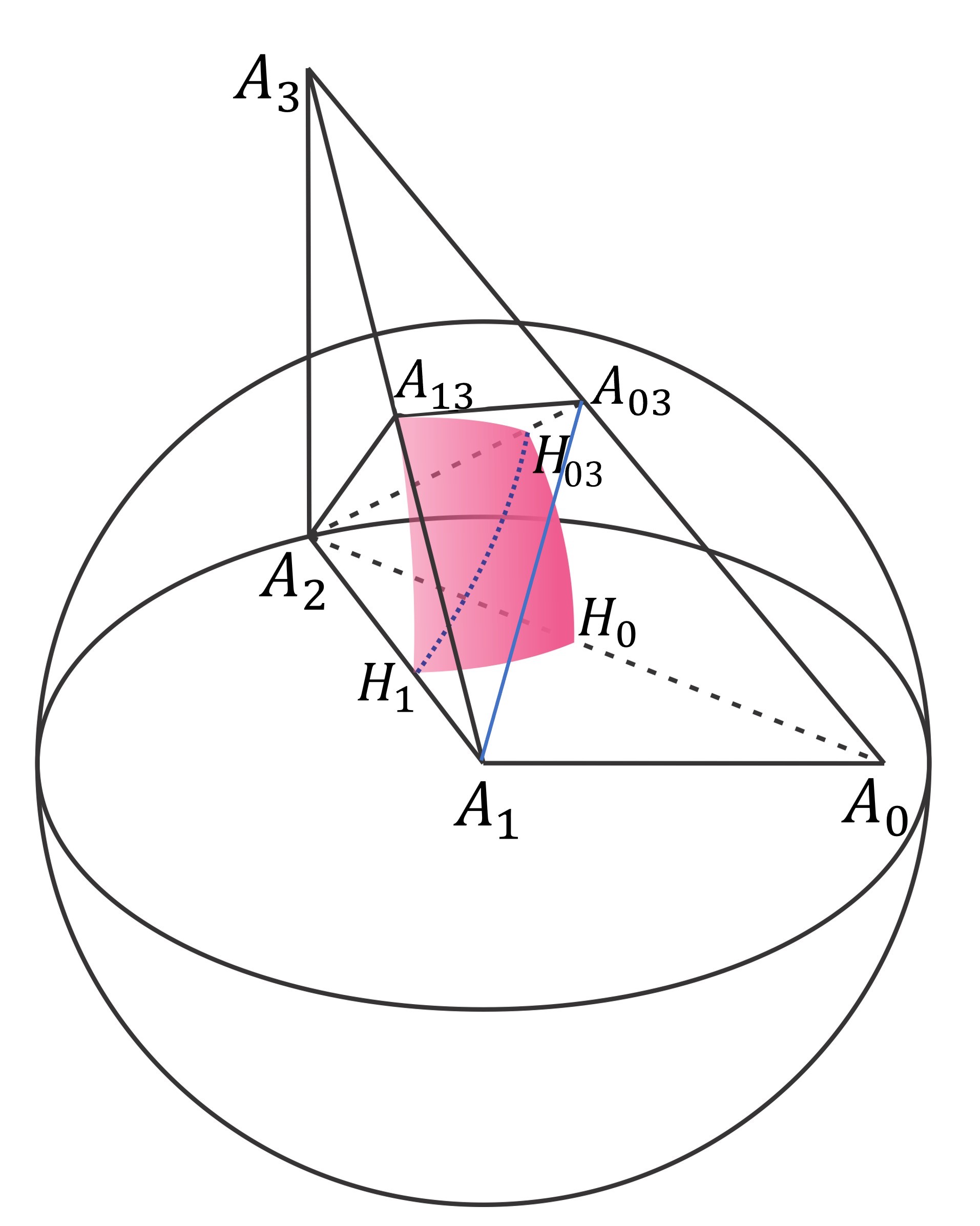
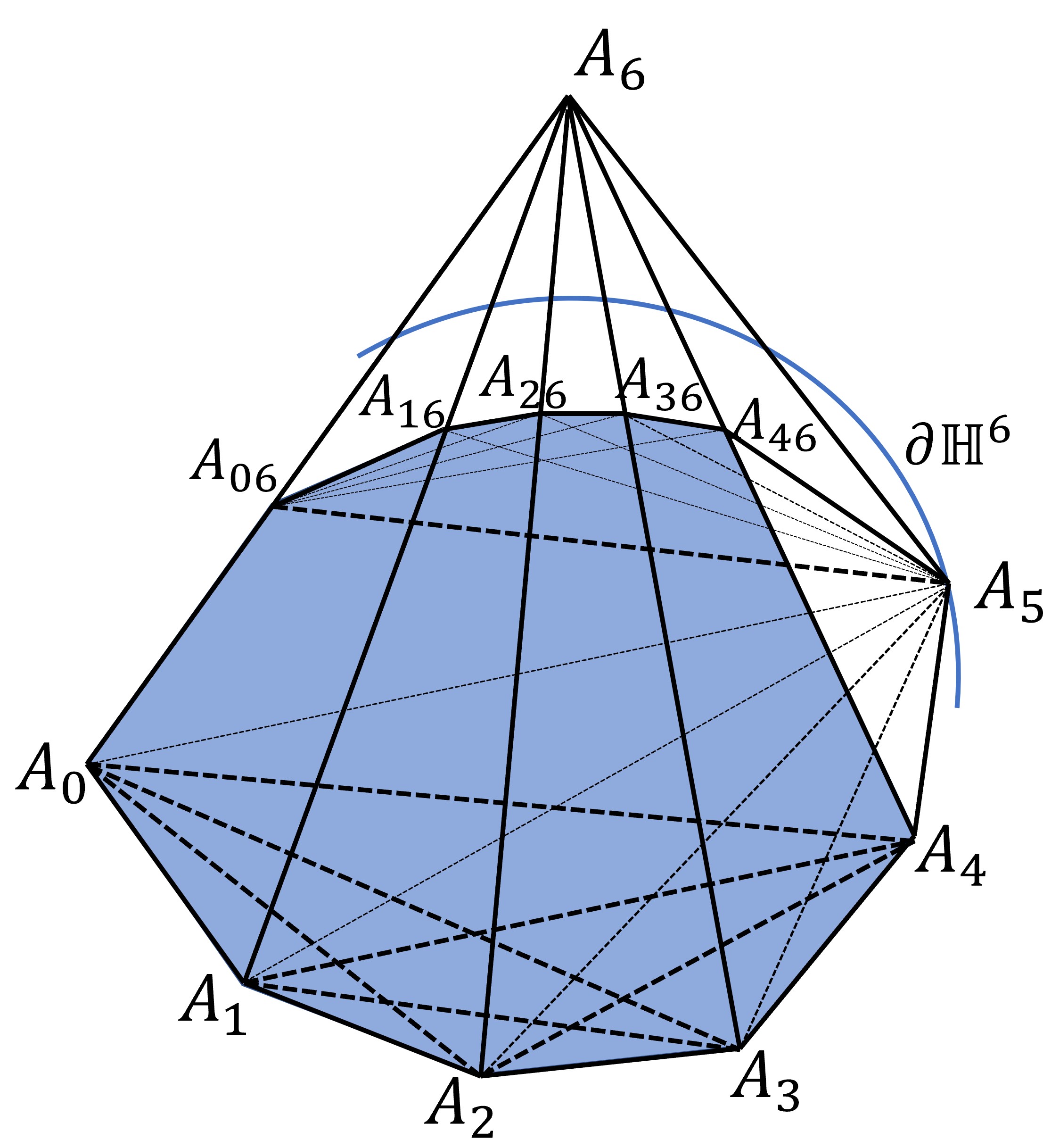
   Figure 5: The horosphere $\mathcal{B}_{2}$ touch its opposite face and the obtained horospherical polyhedron ${A}_{13}{H}_{0}{H}_{1}{H}_{03}$ is dissected into two simplices ${H}_{0}{H}_{1}{H}_{03}$ and ${A}_{13}{H}_{1}{H}_{03}$ through hyperplane ${A}_{2}{A}_{1}{A}_{03}$ in the $3$-dimensional hyperbolic space $\overline{\mathbb{H}}^{3}$ (left). The “Opposite” faces of $A_{5}$ (in the shaded region), indicated by vertices $A_{0}$, $A_{1}$, $A_{2}$, $A_{3}$, $A_{4}$ $A_{06}$, $A_{16}$, $A_{26}$, $A_{36}$, $A_{46}$ in a truncated orthoscheme of $\overline{\mathbb{H}}^{6}$ (right).

   The optimal value of the $s$-parameter for the maximal horoball can be determined from the above equations of the horosphere through $A_{n-1}$ and footpoints $\mathbf{f}_{i}^{n-1}$.

   The intersections $[\mathbf{h}_{i}]$ of horosphere $\partial\mathcal{B}_{n-1}$ and the edges of the polytope $\mathcal{F}_{\Gamma}$ are found by parameterizing the edges $\mathbf{h}_{i}(\lambda)=\lambda\mathbf{a}_{n-1}+\mathbf{a}_{i}$ $(i\in\{0,\cdots,n-2,0n,\cdots,(n-2)n\})$ then finding their intersections with $\partial\mathcal{B}_{n-1}$. The volume of the horospherical $(n-1)$-simplex determines the volume of the horoball piece by equation (2.6). The data for the horospherical $(n-1)$-polytope is obtained by finding hyperbolic distances $l_{ij}$ via equation (2.1), $l_{ij}=d(H_{i},H_{j})$ where $d(\mathbf{h}_{i},\mathbf{h}_{j})=\arccos\left(\frac{-\langle\mathbf{h}_{i},\mathbf{h}_{j}\rangle}{\sqrt{\langle\mathbf{h}_{i},\mathbf{h}_{i}\rangle\langle\mathbf{h}_{j},\mathbf{h}_{j}\rangle}}\right)$. Moreover, the horospherical distances $L_{ij}$ are found by formula (2.5).

   We obtain a horospherical $(n-1)$-polytope $\mathcal{P}$ whose edges are known. The intrinsic geometry of a horosphere is Euclidean, so the obtained polytope’s volume is computed in Euclidean sense. The computation of the volume of the above $n$-dimensional polytope is determined using its decomposition into $n$-dimensional simplexes. In $\overline{\mathbb{H}}^{n}$, the opposite faces of ideal vertex $A_{n-1}$ is determined by polytope $\mathcal{P}$ that is formed as a convex hull of $A_{0},\cdots,A_{n-1},A_{0n},\cdots,A_{(n-2)n}$, see shaded region in Fig. 5. This polytope $\mathcal{P}$ can be dissected into $n-1$ simplices as follows:

   $$E_{k}:=conv(A_{0n},\cdots A_{kn},A_{k},\cdots,A_{n-2}),\leavevmode\nobreak\ \leavevmode\nobreak\ \leavevmode\nobreak\ \text{for }k=0,\cdots,n-2$$

   Note that,

   $${int}(E_{k_{1}})\cap{int}(E_{k_{2}}) =\emptyset,\text{for}\leavevmode\nobreak\ k_{1}\neq k_{2},\leavevmode\nobreak\ \text{where}\leavevmode\nobreak\ int(E_{k})\leavevmode\nobreak\ \text{denote the interior of}E_{k}$$

   $$\text{and}\bigcup_{k=0}^{n-2}E_{k} =\mathcal{P}.$$

   For instance, in $\overline{\mathbb{H}}^{6}$, the polytope $\mathcal{P}$ and its dissected simplices are sketched in Fig. 5.left and 6 respectively.

   

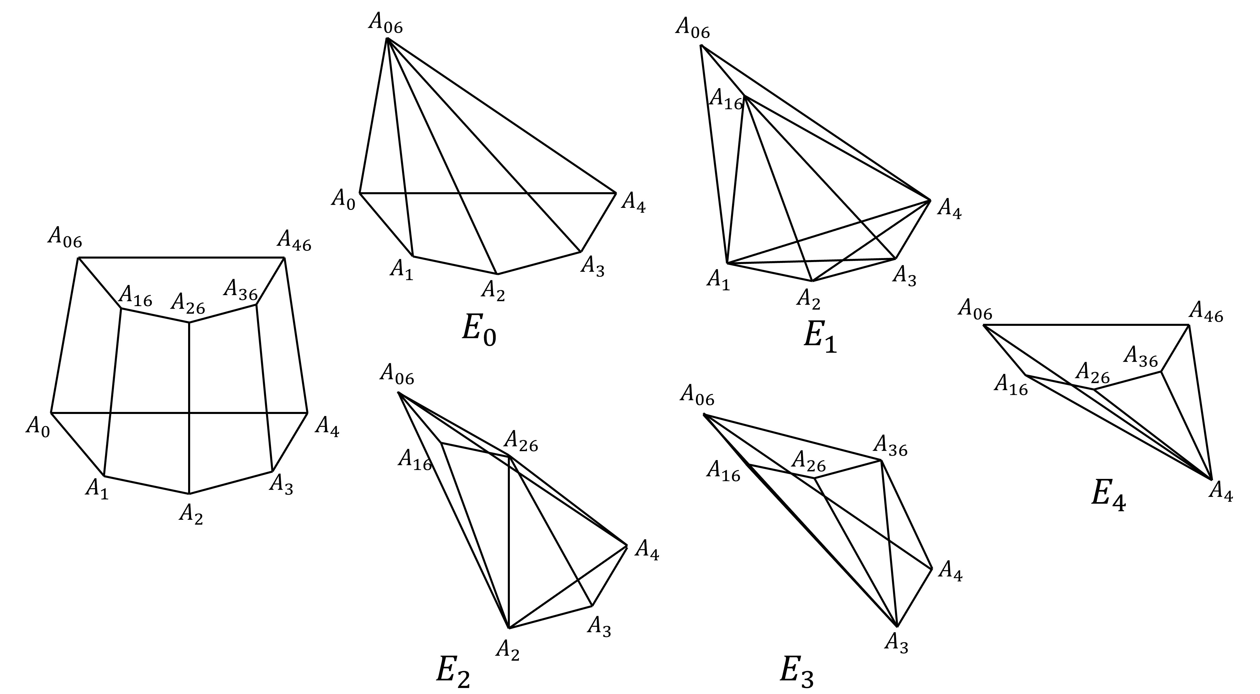
   Figure 6: Sketch of the dissection of $5$-dimensional hyperbolical polytope $\mathcal{P}$ into $5$-dimensional simplices $E_{k}$, $k=0,\cdots 4$.

   Furthermore, we take the point projection of each simplex $E_{k}$ onto the horosphere $\partial\mathcal{B}_{n-1}$ by taking the intersection of $\partial\mathcal{B}_{n-1}$ and the geodesic emanating from the ideal vertex $A_{n-1}$ to all vertices of $\mathcal{P}$. We denote the projection of $E_{k}$ by $D_{k}$, respectively. To calculate the volumes of simplexes $D_{0}\dots D_{n-2}$, we use the Cayley-Menger determinant that gives the volume of a horospherical $(n-1)$-simplex $\mathrm{vol}(\mathcal{A})$ with edges length $L_{i,j}$ ($i=1\dots(n-1),j=2\dots n,i<j$).

   $$\mathrm{vol}(\mathcal{A})^{2}=\frac{1}{(n!)^{2}2^{n}}\begin{vmatrix}0&1&1&1&\dots&1\\ 1&0&L_{1,2}^{2}&L_{1,3}^{2}&\dots&L_{1,n}^{2}\\ 1&L_{1,2}^{2}&0&L_{2,3}^{2}&\dots&L_{2,n}^{2}\\ \vdots&\vdots&\vdots&\ddots&\dots&\vdots\\ 1&L_{1,n}^{2}&L_{2,n}^{2}&\dots&L_{n-1,n}^{2}&0\end{vmatrix}.$$ (4.4)

   The volume of the horoball piece contained in the fundamental simplex is

   $$\mathrm{vol}(\mathcal{B}_{n-1}\cap\mathcal{F}_{\Gamma})=\frac{1}{n-1}\mathrm{vol}(\mathcal{Q}),\leavevmode\nobreak\ \leavevmode\nobreak\ \text{where}\leavevmode\nobreak\ \mathcal{Q}:=\bigcup_{k=0\cdots n-2}D_{k}$$ (4.5)

   The locally optimal horoball packing density of Coxeter Simplex $\mathcal{F}_{\Gamma}$ can be determined by formula $\delta_{opt}(\mathcal{F}_{\Gamma})=\frac{\mathrm{vol}(\mathcal{B}_{n-1}\cap\mathcal{F}_{\Gamma})}{\mathrm{vol}(\mathcal{F}_{\Gamma})}$.

   The above local construction is preserved by the isometric actions of $g\in\Gamma$. The Coxeter group $\Gamma$ extends the optimal local horoball packing density from the fundamental domain $\mathcal{F}_{\Gamma}$ to the entire tiling $\mathcal{T}_{\Gamma}$ of $\overline{\mathbb{H}}^{n}$ therefore we obtain the horoball packing density of the considered tiling by formulas (4.1) and (4.2)).

   Remark 4.1

   In some cases, there may be an additional ideal vertex $A_{0}$, allowing us to consider a horosphere centered at this vertex. The process of determining the density of the optimal horoball packing in these cases is similar to the previously described case. Furthermore, the $(n-1)$-dimensional horospherical polytope $\mathcal{Q}$ is a simplex in these cases, and its volume $\mathrm{vol}(\mathcal{Q})$ can be calculated directly using the Cayley-Menger determinant.

2. Two horoball types The computational method for determining the optimal horoball sectors and their volumes is similar to the ”one horoball type” method described above. However, in the investigated cases, the two horoballs cannot have a common interior point. At most, they can be tangent to each other. The volumes of the two tangent horoball pieces, centered at two distinct ideal vertices of the fundamental domain, as the horoball type is continuously varied, are related in Lemma 4.2.

   In $\overline{\mathbb{H}}^{n}$ with $n\geq 2$ let $\tau_{1}$ and $\tau_{2}$ be two congruent $n$-dimensional convex cones with vertices at $C_{1},C_{2}\in\partial\overline{\mathbb{H}}^{n}$ that share a common geodesic edge $\overline{C_{1}C_{2}}$. Let $B_{1}(x)$ and $B_{2}(x)$ denote two horoballs centered at $C_{1}$ and $C_{2}$ respectively, mutually tangent at $I(x)\in{\overline{C_{1}C_{2}}}$. Define $I(0)$ as the point with $V(0)=2\mathrm{vol}(B_{1}(0)\cap\tau_{1})=2\mathrm{vol}(B_{2}(0)\cap\tau_{2})$ for the volumes of the horoball sectors.

   Lemma 4.2 ([33])

   Let $x$ be the hyperbolic distance between $I(0)$ and $I(x)$, then

   $$\begin{split}V(x)=&\mathrm{vol}(B_{1}(x)\cap\tau_{1})+\mathrm{vol}(B_{2}(x)\cap\tau_{2})\\ =&V(0)\frac{e^{(n-1)x}+e^{-(n-1)x}}{2}=V(0)\cosh\left((n-1)x\right)\end{split}$$ (4.6)

   is strictly convex and strictly increasing as $x\rightarrow\pm\infty$.

   See our paper [33] for a proof.

   The methods described above can be used to determine the optimal horoball packings and their densities.

4.2 Results related to horoball packings

4.2.1 Horoball packings in $\overline{\mathbb{H}}^{4}$

1. Packings with one horoball

   In the given scenario, we consider a horosphere centered at $A_{3}$. As mentioned, the horosphere packing reaches its optimal density when the horosphere is tangent to the opposite faces, which are determined by the vertices $A_{0},A_{1},A_{2},A_{04},A_{14},A_{24}$. This optimal packing configuration is realized in all possible tilings, as indicated by the Schläfli symbols in Fig. 1.

   In the case of the Schläfli symbol ${4,4,3,4,\infty}$, there are two ideal vertices, namely $A_{0}$ and $A_{3}$. Therefore, we can construct another horosphere centered at vertex $A_{0}$. This horosphere packing will be optimal when it is tangent to the opposite face of $A_{0}$, which is determined by the vertices $A_{1},A_{2},A_{3},A_{4}$.

   By applying the previously described method, as well as formulas (4.3), (4.4), and (4.5), and utilizing the volume values described in Table 2, we have summarized the results in Table 6.

   [.5]() Schläfli symbol	$\mathrm{vol}(\mathcal{B}_{i}\cap\widehat{\mathcal{S}})$	$\mathrm{vol}(\widehat{\mathcal{S}})$	$\delta_{opt}(\mathcal{B}_{\Gamma})$.
   [.5]() $\{4,4,3,3,\infty\},\leavevmode\nobreak\ i=3$	$\frac{1}{48}$	$\frac{\pi^{2}}{288}$	$\frac{6}{\pi^{2}}\approx 0.60793$
   [.5]() $\{4,4,3,4,\infty),\leavevmode\nobreak\ i=3$	$\frac{\sqrt{2}}{48}$	$\frac{\pi^{2}}{144}$	$\frac{3}{8\pi^{2}}\approx 0.42987$
   [.5]() $\{4,4,3,4,\infty\},\leavevmode\nobreak\ i=0$	$\frac{\sqrt{2}}{72}$	$\frac{\pi^{2}}{144}$	$\frac{2\sqrt{2}}{\pi^{2}}\approx{0.28658}$
   [.5]() $(6,3,3,3,\infty\},\leavevmode\nobreak\ i=3$	$\frac{\sqrt{3}}{144}$	$\frac{\pi^{2}}{540}$	$\frac{15\sqrt{3}}{4\pi^{2}}\approx\textbf{0.65810}$
   [.5]() $\{6,3,3,4,\infty\},\leavevmode\nobreak\ i=3$	$\frac{\sqrt{6}}{144}$	$\frac{\pi^{2}}{288}$	$\frac{2\sqrt{6}}{\pi^{2}}\approx 0.49637$
   [.5]() $\{6,3,3,5,\infty\},\leavevmode\nobreak\ i=3$	$\frac{1}{48}\sqrt{\frac{3+\sqrt{5}}{6}}$	$\frac{61\pi^{2}}{900}$	$\frac{25(\sqrt{3}+\sqrt{15})}{244\pi^{2}}\approx 0.02909$
   [.5]() $\{6,3,4,3,\infty\},\leavevmode\nobreak\ i=3$	$\frac{\sqrt{3}}{72}$	$\frac{5\pi^{2}}{864}$	$\frac{12\sqrt{3}}{5\pi^{2}}\approx 0.42119$

   Table 6: Horoball Packing densities in $\overline{\mathbb{H}}^{4}$, with one horosphere

2. Packings with two horoballs

   Theorem 4.3

   The optimal horoball packing density of Coxeter simplex tilings $\mathcal{T}_{\Gamma}$ where $\Gamma$ is determined by Schläfli symbol $\{4,4,3,4,\infty\}$ is

   $$\delta_{opt}(\mathcal{T}_{\Gamma})=\frac{\mathrm{vol}(\mathcal{B}_{0}^{opt}\cap\widehat{\mathcal{S}})+\mathrm{vol}(\mathcal{B}_{3}^{opt}\cap\widehat{\mathcal{S}}))}{\frac{\pi^{2}}{144}}\approx 0.71645.$$ (4.7)

   Proof
   We consider the case of Schläfli symbol $\{4,4,3,4,\infty\}$ whose the Coxeter-Schläfli matrix is the following Gram matrix

   $$(b^{ij})=(\langle\boldsymbol{b}^{i},\boldsymbol{b}^{j}\rangle)=\left[\begin{matrix}1&-\frac{\sqrt{2}}{2}&0&0&0\\ -\frac{\sqrt{2}}{2}&1&-\frac{\sqrt{2}}{2}&0&0\\ 0&-\frac{\sqrt{2}}{2}&1&-\frac{1}{2}&0\\ 0&0&-\frac{1}{2}&1&-\frac{\sqrt{2}}{2}\\ 0&0&0&-\frac{\sqrt{2}}{2}&1\end{matrix}\right],$$ (4.8)

   where $0\leq i,j\leq 4$. Moreover, the corresponding inverse matrix $(a_{ij})$

   $$(a_{ij})=(\langle\boldsymbol{b}^{i},\boldsymbol{b}^{j}\rangle)^{-1}=\left[\begin{matrix}0&-\sqrt{2}&-2&-2&-\sqrt{2}\\ -\sqrt{2}&-2&-2\sqrt{2}&-2\sqrt{2}&-2\\ -2&-2\sqrt{2}&-2&-2&-\sqrt{2}\\ -2&-2\sqrt{2}&-2&0&0\\ -\sqrt{2}&-2&-\sqrt{2}&0&1\end{matrix}\right]$$ (4.9)

   shows that the truncated orthoscheme has two ideal vertices $A_{0}[\mathbb{a}_{0}]$, and $A_{3}[\mathbb{a}_{3}]$ since $a_{00}=0$, and $a_{33}=0$. We have an ultra ideal vertices $A_{4}[\mathbb{a}_{4}]$, since $a_{44}=1>0$.
   First, we choose the set unit normal forms of the orthoscheme hyperplane faces $\boldsymbol{b}^{0}=(0,0,1,0,0)^{T}$, $\boldsymbol{b}^{1}=(-\frac{\sqrt{2}}{2},,-\frac{\sqrt{2}}{2},-\frac{\sqrt{2}}{2},-\frac{\sqrt{2}}{2},0)^{T}$, $\boldsymbol{b}^{2}=(0,0,0,1,0)^{T}$, $\boldsymbol{b}^{3}=(0,\frac{1}{2},0,-\frac{1}{2},-\frac{\sqrt{2}}{2})^{T}$, $\boldsymbol{b}^{4}=(0,0,0,0,1)^{T}$ admitted the Gram matrix (Coxeter Schläfli Matrix) (4.8).
   Those unit normal vectors $\{\boldsymbol{b}^{0},\boldsymbol{b}^{1},\boldsymbol{b}^{2},\boldsymbol{b}^{3},\boldsymbol{b}^{4}\}$ and $(a_{ij})$ determine the orthoscheme vertices whose coordinates: $\mathbb{a}_{0}=(1,0,1,0,0)$, $\mathbb{a}_{1}=(1,0,0,0,0)$, $\mathbb{a}_{2}=(1,\frac{1}{2},0,\frac{1}{2},0)$, $\mathbb{a}_{3}=(1,1,0,0,0)$, $\mathbb{a}_{4}=(1,1,0,0,\frac{\sqrt{2}}{2})$. We consider two horoballs $\mathcal{B}_{0}$ and $\mathcal{B}_{3}$ centred at $A_{0}$ and $A_{3}$ which hold the packing conditions, so they may touch each other at a point on edge $A_{0}A_{3}$. To investigate this possibility, we consider a linear parametrization of moving point $P[\mathbf{p}]$ points on $A_{0}A_{3}$

   $$\mathbb{p}(t)=(1-t)\mathbb{a}_{3}+t\mathbb{a}_{0},\qquad t\in[0,1],$$ (4.10)

   where clearly $\mathbb{p}(0)=\mathbb{a}_{3}$ and $\mathbb{p}(1)=\mathbb{a}_{0}$. Based on the method described in subsection 4.1 we can determine possible maximal horospheres centred at $A_{0}$ and $A_{3}$ and its parameters $s_{i},i\in\{0,3\}$ using the projection formula (4.3) and the equation of horospheres given in (2.4).

   $$\mathbf{f}_{3}=\mathbf{a}_{3}-\frac{\langle\mathbf{a}_{3},\mathbf{b}^{3}\rangle}{\langle\boldsymbol{b}^{3},\boldsymbol{b}^{3}\rangle}\mathbf{b}^{3}=\left(1,\frac{3}{4},0,\frac{1}{4},\frac{\sqrt{2}}{4}\right)$$

   An isometry could take $A_{3}$ to the point $(1,0,0,0,1)$, and $\mathbb{f}_{3}$ to $\hat{\mathbb{f}}_{3}=(1,\frac{\sqrt{2}}{4},\frac{1}{4},0,\frac{3}{4})$ by substituting $\hat{\mathbb{f}}_{3}$ to the horosphere equation given in (2.4), we have

   $$\frac{\left(\frac{1}{2}-s\right)^{2}}{\left(1-s\right)^{2}}+\frac{\frac{3}{8}}{1-s}=1$$

   by solving the last equation for $s$, then it is concluded that $s_{3}=\frac{3}{5}$, furthermore the corresponding $t$ in (4.10) is $t_{3}=\frac{1}{3}$, i.e., $\mathbb{p}(\frac{1}{3})$ is the intersection of $\mathcal{B}_{3}$ and the edge $A_{3}A_{0}$.
   On the other hand, We consider the horoball $\mathcal{B}_{0}$ centred at $A_{0}$ such that it tangent either the opposite face, $H_{0}$ determined by vertices $A_{1},A_{2},A_{3},A_{4}$ or the truncation face $H_{5}$ given by vertices $A_{04},A_{14},A_{24},A_{3}$. We consider the following projections:

   $$\mathbf{f}_{0}=\mathbf{a}_{0}-\frac{\langle\mathbf{a}_{0},\mathbf{b}^{0}\rangle}{\langle\boldsymbol{b}^{0},\boldsymbol{b}^{0}\rangle}\mathbf{b}^{0}=(1,0,0,0,0)=\mathbf{a}_{1}$$

   There is an isometry that takes $\mathbf{a}_{0}$ to $(1,0,0,0,1)$, where $\mathbb{f}_{0}=\mathbf{a}_{1}$ is the fix point. By substituting $\mathbb{f}_{0}$ into the equation (2.4), and solving the equation for $s$ we obtain $s_{0}=0$. This parameter $s_{0}=0$ determine the horosphere $\mathcal{B}_{0}^{opt}$.
   Consider

   $$\mathbb{q}(t)=(1-t)\mathbb{a}_{0}+t\mathbb{a}_{3},\leavevmode\nobreak\ \leavevmode\nobreak\ t\in[0,1]$$

   this is obviously the opposite of $\mathbb{p}$, i.e., $\mathbb{q}(t)=\mathbb{p}(1-t)$. By careful analysis, the intersection of $\mathcal{B}_{0}(s_{0})$ and the edge $A_{0}A_{3}$ is the point $\mathbb{q}(\frac{2}{3})$. As a result,

   $$\mathbb{q}\left(\frac{2}{3}\right)=\mathbb{p}\left(1-\frac{2}{3}\right)=\mathbb{p}\left(\frac{1}{3}\right)$$

   that means the horoballs $\mathcal{B}_{0}^{opt}$ and $\mathcal{B}_{3}^{opt}$ touch each other at a point on edge $A_{0}A_{3}$.

   The optimum density of horoball packing with two horospheres can be directly computed by (4.4) and (4.5)

   $$\begin{gathered}\delta_{opt}(\mathcal{T}_{\Gamma})=\frac{\mathrm{vol}(\mathcal{B}_{0}^{opt}\cap\widehat{\mathcal{S}})+\mathrm{vol}(\mathcal{B}_{3}^{opt}\cap\widehat{\mathcal{S}}))}{\frac{\pi^{2}}{144}}\\ =\frac{\mathrm{vol}(\mathcal{B}_{0}(0)\cap\widehat{\mathcal{S}})+\mathrm{vol}(\mathcal{B}_{3}(\frac{3}{5})\cap\widehat{\mathcal{S}}))}{\frac{\pi^{2}}{144}}=\frac{\frac{\sqrt{2}}{48}+\frac{\sqrt{2}}{72}}{\frac{\pi^{2}}{144}}=\frac{5\sqrt{2}}{\pi^{2}}\approx 0.71645\leavevmode\nobreak\ \leavevmode\nobreak\ \leavevmode\nobreak\ \square\end{gathered}$$

   Finally, we summarize our results in the following theorem

   Theorem 4.4

   In hyperbolic space $\overline{\mathbb{H}}^{4}$, between the congruent ball and horoball packings of at most two horoball types, generated by simply truncated Coxeter orthoschemes with parallel faces, the above determined $\mathcal{B}_{\{4,4,3,4,\infty\}}$ horoball configuration provides the densest packing with density $\frac{5\sqrt{2}}{\pi^{2}}\approx 0.71645$.

   Remark 4.5

   This density $\delta_{opt}(\mathcal{T}_{\Gamma})\approx 0.71645$ is the known densest horoball packing density in $\overline{\mathbb{H}}^{4}$. We note here, that this density is realized in seven asymptotic Coxeter simplex tilings $\Gamma\in\{\overline{S}_{4},\overline{P}_{4},\widehat{FR}_{4},\overline{N}_{4},\overline{M}_{4},\overline{BP}_{4},$ $\overline{DP}_{4}\}$, if horoballs of different types are allowed at each asymptotic vertex of the tiling (see [19]).

4.2.2 Horoball packings in $\overline{\mathbb{H}}^{5}$

The Coxeter Schläfli matrix of orthoscheme whose Schläfli symbol $\{4,3,4,3,3,\infty\}$ is $(b^{ij})$. Choosing the unit normal forms of hyperplane faces of the orthoscheme admitted the matrix $(b^{ij})$, i.e.,

$$\begin{gathered}\boldsymbol{b}^{0}=(0,0,1,0,0,0)^{T},\boldsymbol{b}^{1}=\left(-\frac{\sqrt{15}}{3}-\sqrt{3},-\frac{3\sqrt{2}}{2}-\frac{\sqrt{10}}{2},-\frac{\sqrt{2}}{2},-\frac{1}{2},0,0\right)^{T},\\ \boldsymbol{b}^{2}=(0,0,0,1,0,0)^{T},\boldsymbol{b}^{3}=\left(\frac{\sqrt{30}}{6},1,0,-\frac{\sqrt{2}}{2},-\frac{\sqrt{3}}{3},0\right)^{T},\\ \boldsymbol{b}^{4}=\left(0,0,0,0,\frac{\sqrt{3}}{2},-\frac{1}{2}\right)^{T},\boldsymbol{b}^{5}=(0,0,0,0,0,1)^{T}.\end{gathered}$$ (4.11)

The corresponding vertices are given by $A_{0}[\boldsymbol{a}_{0}]$, $A_{1}[\boldsymbol{a}_{1}],$ $A_{2}[\boldsymbol{a}_{2}]$, $A_{3}[\boldsymbol{a}_{3}],A_{4}[\boldsymbol{a}_{4}],$ $A_{5}[\boldsymbol{a}_{5}]$, where

$$\begin{gathered}\mathbf{a}_{0}=\left(1,\frac{\sqrt{30}}{6},\frac{\sqrt{6}}{6},0,0,0\right),\mathbf{a}_{1}=\left(1,\frac{\sqrt{30}}{6},0,0,0,0\right),\\ \mathbf{a}_{2}=\left(1,\frac{2\sqrt{6}+5\sqrt{30}}{33},0,\frac{4\sqrt{3}-\sqrt{15}}{33},0,0\right),\mathbf{a}_{3}=\left(1,\frac{\sqrt{6}+\sqrt{30}}{8},0,0,0,0\right)\\ \mathbf{a}_{4}=\left(1,\frac{\sqrt{6}+\sqrt{30}}{8},0,0,\frac{3\sqrt{2}-\sqrt{10}}{8},0\right),\\ \mathbf{a}_{5}=\left(1,\frac{\sqrt{6}+\sqrt{30}}{8},0,0,\frac{3\sqrt{2}-\sqrt{10}}{8},\frac{3\sqrt{6}-\sqrt{30}}{8}\right).\end{gathered}$$ (4.12)

1. Packings with one horoball

   Figure 2 illustrates that in the $5$-dimensional hyperbolic space $\overline{\mathbb{H}}^{5}$, there is only one Coxeter tiling $\mathcal{T}_{\Gamma}$ generated by a simply truncated orthoscheme with parallel faces of Schläfli symbol ${4,3,4,3,3,\infty}$. By observing the corresponding $(a{ij})=(b^{ij})^{-1}$ matrix, we note that its fundamental domain $\mathcal{F}_{\Gamma}$ has two ideal vertices, $A_{0}$ and $A_{4}$. Hence, we can construct horoballs centered at either of these ideal vertices. In the case of the horosphere centered at $A_{0}$, the opposite face is $A_{1}A_{2}A_{3}A_{4}A_{5}$, and the truncation face is $A_{4}A{05}A_{15}A_{25}A_{35}$. However, the optimal packing configuration can only be realized when the horosphere touches the face $A_{1}A_{2}A_{3}A_{4}A_{5}$. Similar to the $4$-dimensional case described above, by applying formulas (4.3), (4.4), (4.5), and the volume value determined in subsection 2.3.2, we can determine the densest horoball packings with one horoball type. The results are summarized in Table 7.

   [.5]() Schläfli symbol	$\mathrm{vol}(\mathcal{B}_{i}\cap\widehat{\mathcal{S}})$	$\mathrm{vol}(\widehat{\mathcal{S}})$	$\delta_{opt}(\mathcal{B}_{\Gamma})$.
   [.5]() $\{4,3,4,3,3,\infty\},\leavevmode\nobreak\ i=4$	$\frac{1}{384}$	$\frac{7\zeta{(3)}}{1152}$	$\frac{3}{7\zeta{(3)}}\approx\mathbb{0.35653}$
   [.5]() $\{4,3,4,3,3,\infty\},\leavevmode\nobreak\ i=0$	$\frac{1}{576}$	$\frac{7\zeta{(3)}}{1152}$	$\frac{2}{7\zeta{(3)}}\approx 0.23769$

   Table 7: Packing densities in $\overline{\mathbb{H}}^{5}$, with one horoball

2. Packings with two horoballs

   Here we consider two horospheres centered at $A_{0}$ and $A_{4}$ together and compute their optimal arrangements and density. It is analogous to the previous construction in $4$-dimensional hyperbolic space (see 4.2.1 subsection). We define the following linear parametrization

   $$\mathbb{p}(t)=(1-t)\mathbb{a}_{4}+t\mathbb{a}_{0},\ \ t\in[0,1],$$ (4.13)

   that describes points along edge $A_{0}A_{4}$. By careful investigation, we find that if $t=\frac{27-6\sqrt{5}}{61}$, then the horosphere centred at $A_{4}$ osculates the opposite face. Furthermore, this exact value of $t$ provides the conditions of the other horosphere centred at $A_{0}$ osculate the opposite face $A_{1}A_{2}A_{3}A_{4}A_{5}$. Therefore, these two horospheres tangent each other if and only if they osculate their centres opposite faces. We summarize the computation result in Table 8.

   [.5]() Schläfli symbol	$\mathrm{vol}((\mathcal{B}_{0}\cup\mathcal{B}_{4})\cap\widehat{\mathcal{S}})$	$\mathrm{vol}(\widehat{\mathcal{S}})$	$\delta_{opt}(\mathcal{B}_{\Gamma}))$.
   [.5]() $(4,3,4,3,3,\infty),\leavevmode\nobreak\ i=0,4$	$\frac{5}{1152}$	$\frac{7\zeta{(3)}}{1152}$	$\frac{5}{7\zeta{(3)}}\approx\mathbb{0.59421}$

   Table 8: Packing densities in $\overline{\mathbb{H}}^{5}$, with two horoballs

   We summarize our investigation in 5-dimensional case with the following theorem.

   Theorem 4.6

   In hyperbolic space $\overline{\mathbb{H}}^{5}$, between the congruent ball and horoball packings of at most two horoball types, generated by simply truncated Coxeter orthoschemes with parallel faces, the above determined $\mathcal{B}_{\{4,3,4,3,3,\infty\}}$ horoball configuration provides the densest packing with density $\frac{5}{7\zeta{(3)}}\approx 0.59421$.

Remark 4.7

In [20] we proved that the above optimal density is realized in ten commensurable asymptotic Coxeter simplex tilings

$$\Gamma\in\left\{\overline{U}_{5},\overline{S}_{5},\overline{Q}_{5},\overline{X}_{5},\overline{R}_{5},\overline{N}_{5},\overline{O}_{5},\overline{M}_{5},\overline{L}_{5},\widehat{UR}_{5}\right\},$$

when horoballs of different types are allowed at each asymptotic vertex of the tiling.

4.2.3 Horoball packings in $\overline{\mathbb{H}}^{6}$

1. Packings with one horoball

   Tha Fig. 2 shows that in the $6$-dimensional hyperbolic space $\overline{\mathbb{H}}^{6}$ there are two Coxeter tiling $\mathcal{T}_{\Gamma_{i}},\leavevmode\nobreak\ i\in\{1,2\}$ generated by simply truncated orthoschemes with parallel faces of Schäfli symbols $\{3,4,3,3,3,3,\infty\}$ and $\{3,4,3,3,3,4,$ $\infty\}$. Using the corresponding $(a_{ij})=(b^{ij})^{-1}$ matrices it is clear, that in the first case the fundamental domain $\mathcal{F}_{\Gamma_{1}}$ has only one ideal vertex $A_{5}$ and in the second case the fundamental domain $\mathcal{F}_{\Gamma_{1}}$ has has two ideal vertices, $A_{0}$ and $A_{5}$. Hence, we can construct horoballs centred at either ideal vertices. The horosphere should be created, centred at ideal vertex $A_{5}$, as mentioned in the previous subsections. Furthermore, in configuration of Schläfli symbol $\{3,4,3,3,3,4,\infty\}$, we have another horosphere centred at $A_{0}$. The horoball sector centred at $A_{0}$ will reach maximum volume, if it osculates the opposite face of $A_{0}$, i.e., the face $A_{1}A_{2}A_{3}A_{4}A_{5}A_{6}$. On the other hand, the hull of vertices $A_{1}A_{2}A_{3}A_{4}A_{5}A_{6}$ is an 5-simplex in $\overline{\mathbb{H}}^{6}$. We can take the central projection of this simplex on the horosphere, and compute the volume of its horoball sector. Similarly to the above $4$- and $5$-dimensional case applying the formulas (4.3), (4.4), (4.5), and the volume values in Table 2. We can determine the densest horoball packings with one horoball type. We summarized the results in Table 9.

   [.5]() Schläfli symbol	$\mathrm{vol}(\mathcal{B}_{i}\cap\hat{\mathcal{S}})$	$\mathrm{vol}(\hat{\mathcal{S}})$	$\delta_{opt}(\mathcal{B}_{\Gamma}))$.
   [.5]() $(3,4,3,3,3,3,\infty),\leavevmode\nobreak\ i=5$	$\frac{1}{23040}$	$\frac{11\pi^{3}}{86400}$	$\approx 0.01010$
   [.5]() $(3,4,3,3,3,4,\infty),\leavevmode\nobreak\ i=5$	$\frac{\sqrt{2}}{23040}$	$\frac{\pi^{3}}{86400}$	$\approx\mathbb{0.17114}$
   [.5]() $(3,4,3,3,3,4,\infty),\leavevmode\nobreak\ i=0$	$\frac{1}{19200}$	$\frac{\pi^{3}}{86400}$	$\approx 0.14513$

   Table 9: Packing densities in $\overline{\mathbb{H}}^{6}$, with one horoballs

2. Packings with two horoballs

   In case of the tiling $\mathcal{T}_{\Gamma_{2}}$ given by Schläfli symbol $\{3,4,3,3,3,4,\infty\}$, we have two ideal vertices $A_{0}$ and $A_{5}$. These two horospheres might tangent each other. The point of tangency lies on the edge $A_{0}A_{5}$ if it exists. We can determine the maximum possible horoballs in the fundamental domain (truncated orthoscheme) $\mathcal{F}_{\Gamma_{2}}$ belonging to the ideal vertices, we find that they have no common point, they are disjoint. Therefore the optimal horoball arrangement is derived from this horoball configuration. The optimum density of horoball packings with two horoballs can be directly computed by

   $$\begin{gathered}\delta_{opt}(\mathcal{T}_{\Gamma_{2}})=\frac{\mathrm{vol}(\mathcal{B}_{0}^{opt}\cap\widehat{\mathcal{S}})+\mathrm{vol}(\mathcal{B}_{5}^{opt}\cap\widehat{\mathcal{S}}))}{\frac{\pi^{3}}{86,400}}=\\ =\frac{\mathrm{vol}(\mathcal{B}_{0}(0)\cap\widehat{\mathcal{S}})+\mathrm{vol}(\mathcal{B}_{5}(\frac{7}{9})\cap\widehat{\mathcal{S}}))}{\frac{\pi^{3}}{86,400}}=\\ =\frac{\frac{\sqrt{2}}{23040}+\frac{1}{19200}}{\frac{\pi^{3}}{86,400}}=\frac{15\sqrt{2}}{4\pi^{3}}+\frac{9}{2\pi^{3}}\approx 0.31617\leavevmode\nobreak\ \leavevmode\nobreak\ \leavevmode\nobreak\ \square\end{gathered}$$

   We summarize our results in the following table and theorem.

   [.5]() Schläfli symbol	$\mathrm{vol}((\mathcal{B}_{0}\cup\mathcal{B}_{5})\cap\hat{\mathcal{S}})$	$\mathrm{vol}(\hat{\mathcal{S}})$	$\delta_{opt}(\mathcal{B}_{\Gamma}))$.
   [.5]() $\{3,4,3,3,3,4,\infty\}$	$\frac{5+3\sqrt{2}}{57600\sqrt{2}}$	$\frac{\pi^{3}}{86400}$	$\approx\mathbb{0.31617}$

   Table 10: Packing densities in $\overline{\mathbb{H}}^{6}$, with two horospheres

   Theorem 4.8

   In hyperbolic space $\overline{\mathbb{H}}^{6}$, between the congruent ball and horoball packings of at most two horoball types, generated by simply truncated Coxeter orthoschemes with parallel faces, the above determined $\mathcal{B}_{\{3,4,3,3,3,4,\infty\}}$ horoball configuration provides the densest packing with density $\frac{15\sqrt{2}+18}{4\pi^{3}}\approx 0.31617$.

The ball, horoball, hyperball packings, and coverings in Thurston geometries as well as in higher dimensional hyperbolic spaces still contain many open questions, which we plan to investigate further, which may lead to further interesting results.

References

- [1] Adams, C.: The Noncompact Hyperbolic 3-Manifold of Minimal Volume. Proceedings of the American Mathematical Society, 100(4) (1987), 601–606.
- [2] Agol, I., Culler, M., Shalen, P. B.: Dehn surgery, homology and hyperbolic volume. Algebraic & Geometric Topology, 6(5) (2006), 2297-2312.
- [3] Böröczky, K.: Packing of spheres in spaces of constant curvature, Acta Math. Acad. Sci. Hungar., 32 (1978), 243–261.
- [4] Böröczky, K., Florian, A.: Über die dichteste Kugelpackung im hyperbolischen Raum, Acta Math. Acad. Sci. Hungar., 15 (1964), 237–245.
- [5] Fejes Tóth, G., Kuperberg, W.: Packing and Covering with Convex Sets, Handbook of Convex Geometry Volume B, eds. Gruber, P.M., Willis J.M., North-Holland, (1983), 799–860.
- [6] Fejes Tóth, G., Fejes Tóth, L., Kuperberg, W.: Ball Packings in Hyperbolic Space, In: Lagerungen. Grundlehren der mathematischen Wissenschaften, Springer, Cham, 360 (2023), 263–270, https://doi.org/10.1007/978-3-031-21800-2-11.
- [7] Fejes Tóth, L.: Regular Figures, Macmillian (New York), 1964.
- [8] Im Hof, H.-C.: A class of hyperbolic Coxeter groups, Expo. Math., 3 (1985), 179–186.
- [9] Im Hof, H.-C.: Napier cycles and hyperbolic Coxeter groups, Bull. Soc. Math. Belgique, 42 (1990), 523–545.
- [10] Jacquemet, M.: The inradius of a hyperbolic truncated n-simplex, Discrete Comput.Geom., 51 (2014), 997–1016.
- [11] Johnson, N.W., Kellerhals, R., Ratcliffe, J.G., Tschants, S.T.: The Size of a Hyperbolic Coxeter Simplex, Transformation Groups, 4/4 (1999), 329–353.
- [12] Kellerhals, R.: Ball packings in spaces of constant curvature and the simplicial density function, Journal für reine und angewandte Mathematik, 494 (1998), 189–203.
- [13] Kellerhals, R.: Volumes of cusped hyperbolic manifolds, Topology, 37/4 (1998), 719–734.
- [14] Kellerhals, R.: On Schläfli’s Reduction Formula, Math.Z, 206 (1991), 193–210
- [15] Kellerhals, R.: Scissors Congruence, the Golden Ratio and Volumes in Hyperbolic 5-Space, Discrete Comput. Geom., 47 (2012), 629–658
- [16] Kellerhals, R.: On the volumes of hyperbolic 5-orthoschemes and the trilogarithm, Commentarii Mathematici Helvetici, 67(1) (1992), 648–663
- [17] Kellerhals, R.: Volumes in hyperbolic 5-space, Geometric and functional analysis, 5 (1995), 640–667
- [18] Kozma, R.T., Szirmai, J.: Optimally dense packings for fully asymptotic Coxeter tilings by horoballs of different types, Monatshefte für Mathematik, 168/1 (2012), 27–47.
- [19] Kozma, R.T., Szirmai, J.: New Lower Bound for the Optimal Ball Packing Density of Hyperbolic 4-space, Discrete Comput. Geom., 53/1 (2015), 182-198.
- [20] Kozma, R.T., Szirmai, J.: New Horoball Packing Density Lower Bound in Hyperbolic 5-space, Geometriae Dedicata, 206/1 (2020), 1–25.
- [21] Kozma, R.T., Szirmai, J.: Horoball Packing Density Lower Bounds in Higher Dimensional Hyperbolic -space for , Geometriae Dedicata, (2023) (to appear).
- [22] Kozma, R.T., Szirmai, J.: Optimal Horoball Packing Densities for Koszul-type tilings in Hyperbolic -space, arXiv:2205.03945. Submitted manuscript, (2023), arXiv:2205.03945.
- [23] Marshall, T. H.: Asymptotic Volume Formulae and Hyperbolic Ball Packing, Annales Academic Scientiarum Fennica: Mathematica, 24 (1999), 31–43.
- [24] Marshall, T.H., Martin, G.J.: Cylinder and horoball packing in hyperbolic space. Annales Academiae Scientiarum Fennicae: Mathematica, 30/1 (2005), 3–48.
- [25] Meyerhoff, R.: Sphere-packing and volume in hyperbolic 3-space. Commentarii Mathematici Helvetici, 61 (1986), 271–278.
- [26] Molnár, E.: The projective interpretation of the eight 3-dimensional homogeneous geometries, Beitr. Algebra Geom., 38(1997), 261–288.
- [27] Molnár, E., Szirmai, J.: Symmetries in the 8 homogeneous 3-geometries, Symmetry Cult. Sci., 21/1-3 (2010), 87–117.
- [28] Molnár, E., Prok, I., Szirmai, J.: Surgeries of the Gieseking hyperbolic ideal simplex manifold, Publ. Math. Debrecen, 99/1-2 (2021), 185–200, DOI: 10.5486/PMD.2021.8995.
- [29] Radin, C.: The symmetry of optimally dense packings, Non-Eucledian Geometries, eds. A. Prékopa, E. Molnár, Springer Verlag, (2006), 197–207, .
- [30] Rogers, C.A.: Packing and Covering, Cambridge Tracts in Mathematics and Mathematical Physics 54, Cambridge University Press, (1964).
- [31] Szirmai, J.: The optimal ball and horoball packings of the Coxeter tilings in the hyperbolic 3-space Beitr. Algebra Geom., 46/2 (2005), 545–558.
- [32] Szirmai, J.: The optimal ball and horoball packings to the Coxeter honeycombs in the hyperbolic d-space Beitr. Algebra Geom., 48/1 (2007), 35–47.
- [33] Szirmai, J.: Horoball packings to the totally asymptotic regular simplex in the hyperbolic n-space, Aequationes mathematicae, 85 (2013), 471–482.
- [34] Szirmai, J.: Horoball packings and their densities by generalized simplicial density function in the hyperbolic space, Acta Math. Hung., 136/1-2 (2012), 39–55.
- [35] Szirmai, J., Yahya, A.: Optimal ball and horoball packings generated by 3-dimensional simply truncated Coxeter orthoschemes with parallel faces, Quaestiones Mathematicae, (2022), 1–21.
- [36] Yahya, A., Szirmai, J.: Visualization of Sphere and Horosphere Packings Related to Coxeter Tilings by Simply Truncated Orthoschemes with Parallel Faces, KoG, 25 (2021), 64–71.