StrAE: Autoencoding for Pre-Trained Embeddings using Explicit Structure

Abstract

This work presents StrAE: a Structured Autoencoder framework that through strict adherence to explicit structure, and use of a novel contrastive objective over tree-structured representations, enables effective learning of multi-level representations. Through comparison over different forms of structure, we verify that our results are directly attributable to the informativeness of the structure provided as input, and show that this is not the case for existing tree models. We then further extend StrAE to allow the model to define its own compositions using a simple localised-merge algorithm. This variant, called Self-StrAE, outperforms baselines that don’t involve explicit hierarchical compositions, and is comparable to models given informative structure (e.g. constituency parses). Our experiments are conducted in a data-constrained ($\approx$10M tokens) setting to help tease apart the contribution of the inductive bias to effective learning. However, we find that this framework can be robust to scale, and when extended to a much larger dataset ($\approx$100M tokens), our 430 parameter model performs comparably to a 6-layer RoBERTa many orders of magnitude larger in size. Our findings support the utility of incorporating explicit composition as an inductive bias for effective representation learning.

1 Introduction

Human understanding of natural language is generally attributed to the understanding of composition. The theory is that smaller constituents (words, tokens) recursively combine into larger constituents (phrases, sentences) in a hierarchically structured manner, and that it is our knowledge of said structure that drives understanding Chomsky (1956); Crain and Nakayama (1987); Pallier et al. (2011); de Marneffe et al. (2006). Compositionality can help drive efficient and effective learning of semantics as it presumes knowledge only of the immediate constituents of a phrase and the process of their composition. However, the models that have come to dominate NLP in recent years generally do not explicitly take this property into account.

Transformers Vaswani et al. (2017) have the capacity to model hierarchical compositions through the self-attention mechanism, whereby tokens can come to represent varying degrees of the surrounding context. However, should such behaviour occur, it is incidental to the training process, as there is no strict requirement for tokens to represent higher-order objects, and tokens are never explicitly merged and compressed with one another. Whether Transformers are able to acquire knowledge of syntax, as understood from the linguistics perspective, remains unclear Kim et al. (2020). However, there is evidence that these models do become increasingly tree-like with sufficient scale and training steps Murty et al. (2022); Jawahar et al. (2019). This raises an interesting question. To what extent is this drive towards tree-likeness responsible for their representation-learning capability? Furthermore, evidence from  Lake et al. (2017) suggests that incorporating appropriate inductive biases towards composition can help bridge the stark disparity between the quantity of data required for learning between ML models and humans, and allow computational models to generalise better. If it is indeed an inductive bias towards hierarchical composition that enables humans to acquire multi-level semantics efficiently, and NLP architectures generally aren’t explicitly tasked with modelling such structure, what happens when they are?

To investigate this, we develop StrAE, a Structured AutoEncoder framework. It takes as input a tree structure that represents a hierarchical composition process, and uses it to directly specify the flow of information from leaves to root (encoder) and back from root to leaves (decoder). To disentangle the effect of structure from other confounding factors, we constrain StrAE to only have access to the information immediately provided to it by the input tree. This means that for a given node the model can only use information from the nodes immediately connected to it (constituents): a property we refer to as faithfulness. Following this, we investigate which training objectives are best suited to enable structured multi-level representation learning, and present a novel application of the contrastive loss to hierarchical tree-like structure.

To investigate the utility of compositional structure for representation learning, we employ a data-constrained setting ($\approx$10 million tokens), and evaluate on a series of tasks that measure semantics at both the sentence and word level. We compare the representations learned by StrAE to a series of baselines consisting of other tree-models which do not enforce faithfulness as rigidly as StrAE  and a series of baselines that do not use explicit structure at all. We also verify that our performance is attributable to the form of composition expressed by the tree structures by comparing results across a range of different input structures.

Finally, to investigate how useful a simple bias towards hierarchical composition is, we extend StrAE to allow it to define its own compositional hierarchy. This variant, called Self-StrAE, utilises the learned representations and the encoder to define its own “merge” sequence, which is then employed as the tree structure for the decoder.

Our results indicate that knowledge of structure is indeed beneficial, and that surprisingly even a simple bias for hierarchical composition leads to promising results. In light of these findings, we then extended our experiments to the 100 million token range and analyse how well Self-StrAE performs in a significantly larger setting. Even more surprisingly, despite solely having 430 non-embedding parameters, Self-StrAE is able to achieve comparable performance to a 6 layer RoBERTa Liu et al. (2019) model with 3.95 million parameters.

2 Model

Figure 1: StrAE operation to encode and decode a sentence. Shared colours indicate shared parameters.

We develop a framework (StrAE) that processes a given sentence to generate multi-level embeddings by faithfully conforming to the given structure. Intuitively, it involves embedding the tokens of a sentence onto the leaves of the structure, composing these embeddings while traversing up the structure to generate the full-sentence embedding, and then traversing back down the structure while decomposing embeddings from parent to children, to finally recover the sentence itself—effectively a structured autoencoder. While this generates embeddings for multiple levels of the sentence as dictated by the structure, it also generates embeddings for a node in two directions—composing upwards and decomposing downwards. The composition embeddings represent the local context for a node, while the decomposition embeddings represent its full context given the sequence.

Denoting embeddings $e_{i}\in\operatorname{{}\mathbb{R}}^{N\times N}$, we distinguish embeddings formed traversing upwards and downwards as $\bar{e}_{i}$ and $\underaccent{\bar}{e}_{i}$ respectively. Encodings for the tokens are denoted as the vertices $w_{i}\in\Delta^{V}$, in a $V$-simplex for vocabulary size $V$. Note that while the token encodings $w_{i}$ are effectively one-hot, reconstructions $\hat{w}_{i}$ can be any point on the simplex—interpreted as a distribution over vertices, and thus the vocabulary, with an argmax retrieving the appropriate token. We define the four core components of StrAE as

$$\Omega_{\Psi} :\Delta^{V}\mapsto\operatorname{{}\mathbb{R}}^{N\times N}$$ (embedding)

$$C_{\Phi} :\operatorname{{}\mathbb{R}}^{N\times N}\times\operatorname{{}\mathbb{R}}^{N\times N}\mapsto\operatorname{{}\mathbb{R}}^{N\times N}$$ (composition)

$$D_{\Theta} :\operatorname{{}\mathbb{R}}^{N\times N}\mapsto\operatorname{{}\mathbb{R}}^{N\times N}\times\operatorname{{}\mathbb{R}}^{N\times N}$$ (decomposition)

$$\Lambda_{\Psi^{\!\intercal}} :\operatorname{{}\mathbb{R}}^{N\times N}\mapsto\Delta^{V}$$ (indexing)

where the subscripts on the functions denote learnable parameters. Table 1 shows the model components and their associated parameters. We assume square embeddings during composition and decomposition, to allow for independent channels to capture different aspects of meaning. Figure 1 shows how the model operates over a given sentence.

Table 1: Definitions of model components following § 2. Functions $\mathrm{square}$ and $\mathrm{flatten}$ transform between column vectors and square matrices. Functions $\mathrm{hcat}$ and $\mathrm{hsplit}$ perform horizontal concatenation and (middle) splitting respectively. $\sigma(\cdot)$ denotes the softmax function. $\phi$ and $\theta$ denote additive biases.

$\Omega_{\Psi}(w_{i})$ $=$	$\mathrm{square}(w_{i}^{\!\intercal}\Psi)$	$\Psi\in\operatorname{{}\mathbb{R}}^{V\times N^{2}}$
$C_{\Phi}(\bar{e}_{c_{1}},\bar{e}_{c_{2}})$ $=$	$\mathrm{hcat}(\bar{e}_{c_{1}},\bar{e}_{c_{2}})\Phi+\phi$	$\Phi\in\mathbb{R}^{2N\times N},\phi\in\mathbb{R}^{N}$
$D_{\Theta}(\underaccent{\bar}{e}_{p})$ $=$	$\mathrm{hsplit}(\underaccent{\bar}{e}_{p}\Theta+\theta)$	$\Theta\in\mathbb{R}^{N\times 2N},\theta\in\mathbb{R}^{2N}$
$\Lambda_{\Psi^{\!\intercal}}(\underaccent{\bar}{e}_{i})$ $=$	$\sigma(\mathrm{flatten}(\underaccent{\bar}{e}_{i})^{\!\intercal}\Psi^{\!\intercal})$	$\Psi\in\mathbb{R}^{V\times\text{N}^{2}}$

Figure 2: Contrastive objective over structure: corresponding node (green) is pulled closer, and other nodes (red) are pushed away.

2.1 Objectives

Given this autoencoding framework, a natural objective to employ is the cross entropy (CE), which simply measures at each leaf node how likely the target token $w_{i}$ is given the reconstructed distribution $\hat{w}_{i}$ over the vocabulary. Given sentence $s_{j}=\langle w_{i}\rangle_{i=1}^{T_{j}}$, this objective is formulated as

$$\mathcal{L}_{\text{CE}}=-\frac{1}{T_{j}}\sum_{i=1}^{T_{j}}w_{i}\cdot\log\hat{w}_{i}.$$ (1)

However, the CE objective places fairly minimal constraints on the embeddings themselves; it only requires the leaf embeddings to be ‘close enough’ for retrieval to be successful. The upward and downward intermediate embeddings are wholly unconstrained, and these can end up being quite different. Given we are learning embeddings for the whole tree, we would like to define an objective over all levels, not just the leaves.

For this purpose, we turn to contrastive loss Chen et al. (2020); Shi et al. (2020); Radford et al. (2021). Contrastive loss involves optimising the embeddings of target pairs so that they are similar to each other and dissimilar to all negative examples. To adapt its use for structured embeddings, we apply the objective so as to task the model with maximising the similarity between corresponding upwards and downwards embeddings $(\bar{e}_{i},\underaccent{\bar}{e}_{i})$ while simultaneously minimising the similarity between all other embeddings. This has the additional attractive characteristic that it forces amortisation of the upwards embeddings $\bar{e}_{i}$—incorporating context from the sentences the word or phrase-segment might have occurred in, as the corresponding downward embedding $\underaccent{\bar}{e}_{i}$ has full-sentence information in it. Figure 2 illustrates an example of this objective.

For a given batch of sentences $s_{j}$, we denote the total number of nodes (internal + leaves) in the associated structure as $M$. We construct a pairwise similarity matrix $A\in\operatorname{{}\mathbb{R}}^{M\times M}$ between normalised upward embeddings $\langle\bar{e}_{i}\rangle_{i=1}^{M}$ and normalised downward embeddings $\langle\underaccent{\bar}{e}_{i}\rangle_{i=1}^{M}$, using the cosine similarity metric (with appropriate flattening of embeddings). Denoting $A_{i\bullet},A_{\bullet{}j},A_{ij}$ the $i\textsuperscript{th}$ row, $j\textsuperscript{th}$ column, and $(i,j)\textsuperscript{th}$ entry of a matrix respectively, we define

$$\mathcal{L}_{\text{cont}}=\frac{-1}{2M}\!\!\left[\!\sum_{i=1}^{M}\log\sigma_{\!\tau}(A_{i\bullet})\!+\!\sum_{j=1}^{M}\log\sigma_{\!\tau}(A_{\bullet{}j})\!\right]\!$$ (2)

where $\sigma_{\!\tau}(\cdot)$ is the tempered softmax (temperature $\tau$), normalising over the unspecified (_∙) dimension. Note that $\mathcal{L}_{\text{cont}}$ extends to the batch setting.

Finally, we initialise our embedding matrix from a uniform distribution with the hyper-parameter r denoting range—corresponding to the finding that contrastive loss seeks to promote uniformity and alignment as established by Wang and Isola (2020).

3 Experimental Setup

We divide our experiments into two separate sections, but both share the same overall setup for pre-training data and evaluation. For pre-training data we take a 500k sentence ($\approx$10M tokens) subset of English Wikipedia and 40k sentence development set. We restrict our pre-training data to this scale in order to measure our efficiency hypothesis presented in the introduction. For evaluation, we assess on three categories of tasks: word level semantics, sentence level semantics, and sentence pair classification, with each aiming to capture separate areas of semantic understanding. On the word level we use Simlex Hill et al. (2015), Wordsim S and Wordsim R Agirre et al. (2009). On the sentence level, we use three tasks from the STS suite Cer et al. (2017); Agirre et al. (2012, 2016), the SICK relatedness dataset Marelli et al. (2014), and for sentence pair classification tasks we use RTE and MRPC taken from the GLUE Benchmark Wang et al. (2019a). Table 2 provides an overview. Note that a subset of the tasks distinguish between similarity and relatedness. Briefly, the former measures semantic similarity, as between “running” and “dancing”, as both words act as verbs. Relatedness measures semantic relationships such as between “running” and “Nike” where the words often co-occur together, but belong to different grammatical categories. Finally, we note that Simlex only measures similarity at the exclusion of relatedness.

All tasks apart from the final two classification tasks are measured using the Spearman correlation of the cosine similarity of model embeddings for each pair and human judgements; classification tasks are measured using accuracy. To emphasise the impact of the pre-training with structure, we do not fine-tune any models for the evaluation tasks, instead keeping them frozen. Where a classifier is required, we fine-tune only a task-specific classification head consisting of a FFN with a 512 dimensional hidden layer and an intermediate Tanh activation function. We choose this setup to match the GLUE Benchmark. For all experiments, we pre-train the models across 5 random seeds and present the averaged performance. Downstream classifiers are themselves also trained across 5 random seeds and the average reported. Additionally, for all experiments we set the embedding dimension to 100. Finally, for all models trained on the word level we filter the vocabulary to exclude words occurring fewer than two times in the data.

Table 2: Overview of Evaluation Tasks

Name	Level	Task	Requires Classifier?
SimLex	Word Level	Semantic Similarity	No
WordSim S	Word Level	Semantic Similarity	No
WordSim R	Word Level	Semantic Relatedness	No
STS 12	Sentence Level	Semantic Similarity	No
STS 16	Sentence Level	Semantic Similarity	No
STS B	Sentence Level	Semantic Similarity	No
SICK R	Sentence Level	Semantic Relatedness	No
MRPC	Sentence Level	Paraphrase Detection	Yes
RTE	Sentence Level	Textual entailment	Yes

Table 3: Comparison of StrAE, IORNN and Tree-LSTM embedding performance on our evaluation suite. Higher is better. All tasks that use Spearman’s $\rho$ have the result * 100 and are marked with a †. Score represents the average across all tasks. All models were trained over five random seeds using constituency parses as input. The pre-training objective is indicated by C or CE, representing contrastive loss or cross entropy respectively. Only results where there is no standard deviation overlap between model performance are bolded.

Model	Simlex †	Wordsim S †	Wordsim R †	STS 12 †	STS 16 †	STS B †	SICK R †	MRPC	RTE	Score
StrAE C	15.54 $\pm$ 0.25	56.1 $\pm$ 0.47	43.77 $\pm$ 1.01	34.59 $\pm$ 2.58	50.4 $\pm$ 0.97	41.83 $\pm$ 2.23	50.3 $\pm$ 0.88	67.24 $\pm$ 0.39	56.16 $\pm$ 1.59	46.21
StrAE CE	17.57 $\pm$ 1.08	50.72 $\pm$ 2.97	36.73 $\pm$ 6.19	5.02 $\pm$ 1.1	25.86 $\pm$ 1.03	7.76 $\pm$ 0.95	39.06 $\pm$ 1.51	67.48 $\pm$ 0.3	53.6 $\pm$ 0.46	33.76
IORNN C	1.9 $\pm$ 0.25	27.29 $\pm$ 0.57	11.29 $\pm$ 0.5	-4.2 $\pm$ 0.97	17.47 $\pm$ 1.14	1.87 $\pm$0.55	30.48 $\pm$ 0.55	67.08 $\pm$ 0.16	55 $\pm$ 1.44	23.13
IORNN CE	24.36 $\pm$ 0.6	57.53 $\pm$ 1.59	36.55 $\pm$ 1.78	-0.17 $\pm$ 0.92	22.68 $\pm$ 0.98	5.04 $\pm$ 0.55	38.41 $\pm$ 0.63	67.24 $\pm$ 0.63	54.28 $\pm$ 0.55	33.99
Tree-LSTM C	6.45 $\pm$ 0.4	37.39 $\pm$ 1.2	20.6 $\pm$ 1.49	-1.34 $\pm$ 1.33	23.95 $\pm$ 0.45	4.25 $\pm$ 1.11	32.9 $\pm$ 0.55	68.16 $\pm$ 0.32	52.76 $\pm$ 1.09	27.24
Tree-LSTM CE	14.23 $\pm$ 2.01	48.7 $\pm$ 3.22	33.24 $\pm$ 3.02	-1.66 $\pm$ 1.29	19.38 $\pm$ 1.21	6.7 $\pm$ 1.04	34.55 $\pm$ 1.15	68 $\pm$ 0.0	52.5 $\pm$ 1.98	30.59

4 Comparing Tree Models

Here, we compare StrAE with two existing tree-architectures. These are the IORNN Le and Zuidema (2014); Drozdov et al. (2019, 2020) and the Tree-LSTM Tai et al. (2015). Both architectures take structure as input and are able to traverse through the tree to learn representations. However, they differ in the constraints they impose on information flow. We conduct our experiments along two different axes: how well do the representations perform, and to what extent do the models discriminate between input structures?

To achieve these evaluations, we parse our pre-training set into three kinds of structure. The first are constituency trees extracted from CoreNLP Manning et al. (2014) and binarised using NLTK Bird et al. (2009). The two other kinds are purely right-branching and balanced binary trees, which we extract using standard algorithms. The resulting structures are then converted to DGL graphs Wang et al. (2020). Hyper-parameter descriptions for each model can be found in Appendix A.

Baselines

The Inside-Outside Recursive Neural Network (IORNN) processes data hierarchically, working from the “inside” to the “outside”. At each node in the tree, an IORNN maintains two vectors: The inside vector $\bar{e}$, which represents the local meaning of a given node, obtained by composing up the tree. The outside vector $\underaccent{\bar}{e}$, represents the context for the given node obtained by decomposing down the tree. While superficially similar to StrAE, the models differ in an important aspect. For given parent $p$ and children $c1$, $c2$ the outside representation:

StrAE:

$\underaccent{\bar}{e}_{c1},\underaccent{\bar}{e}_{c2}=\mathrm{hsplit}(\underaccent{\bar}{e}_{p}\Theta))$, with $\Theta\in\mathbb{R}^{N\times 2N}$

IORNN:

$\underaccent{\bar}{e}_{c1}=\tanh([\underaccent{\bar}{e}_{p};\bar{e}_{c2}]\Theta)$, with $\Theta\in\mathbb{R}^{2N\times N}$

$\underaccent{\bar}{e}_{c2}=\tanh([\underaccent{\bar}{e}_{p};\bar{e}_{c1}]\Theta)$

where $[\cdot;\cdot]$ denotes concatenation. In StrAE the outside representation solely depends on the parent and therefore enforces a compression bottleneck at the root of the structure. No other information may be shared from the composition process, and all $\underaccent{\bar}{e}$ embeddings are created recursively based on the root. The outside vector for IORNN is derived from both the parent and the inside vector of a given child’s sibling node. As the root has no siblings or parent nodes, the outside vector consists of a global bias parameter, intended to represent the context of the whole pre-training corpus. Consequently, IORNN does not enforce a compression bottleneck and information flows between both the local compositional (bottom up) and the global decompositional (top down) contexts.

Our second baseline, the Tree-LSTM, is a recursive variant of the LSTM Hochreiter and Schmidhuber (1997). The main difference is that inputs are processed recursively rather than recurrently. At each node, the inputs for the cell are the children’s hidden and cell states. Here the flow of information differs to StrAE because while StrAE has to compress embeddings according to the order dictated by the input structure, the Tree-LSTM is able to selectively retain information from lower down in the tree according to the cell state. Tree-LSTMs can be applied both bottom up Tai et al. (2015); Choi et al. (2017); Maillard et al. (2017) as encoders, and top down as decoders Xiao et al. (2022); Dong and Lapata (2016). Consequently, they can be pre-trained in the same way as StrAE. Parameter counts for all models can be found in Table 5.

Performance on Constituency Parses

We first evaluate model performance purely on the constituency parse structure, as in theory this should be the most informative. Results can be found in Table 3. We train all models using both objectives for the sake of parity with StrAE. Our results demonstrate that while all models are able to capture word level semantics to some degree, it is only StrAE coupled with the contrastive objective that is able to extend this to sentence level semantics, though StrAE with the cross entropy objective still performs better than the other architectures in this regard. These results indicate that enforcing faithfulness is beneficial in learning multilevel representations. It also follows that the contrastive objective is beneficial for StrAE as it is directly applied to all nodes, and therefore directly optimises the root’s relations to other sentences. In the classification tasks, there appears to be little difference between architectures.

It is clear that the contrastive objective is only useful when the model imposes constraints on information flow, as both baselines do not benefit from it. The objective asks the model to reconstruct each node embedding such that it is distinctive from all other embeddings in the batch. If the LSTM is retaining information in its cell state, it makes this distinction difficult to enforce. IORNN faces difficulties in two regards: the outside representation of the root is a global parameter which makes distinction significantly more difficult, and the sharing of information between sibling nodes. We tested the effects of removing the sharing of information and still found little improvement, possibly because the degree of information sharing between inside and outside representations is so high that it renders the requirement for meaningful compression void.

Evidence of IORNN’s reliance on the information sharing from inside sibling nodes can be seen in its Simlex performance with the cross entropy objective. Simlex actively penalises capturing semantic relatedness, which in the case of IORNN is information that would be provided by the outside vector. Its poor performance indicates that IORNN is not using the parent outside representation as significantly when reconstructing embeddings, which may explain the difficulties on the sentence level tasks as the model can simply try to predict a word given its immediate left or right neighbour.

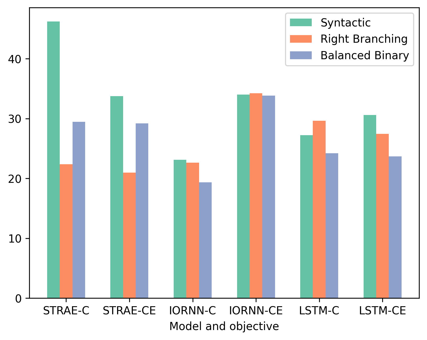
(a) Overall Score

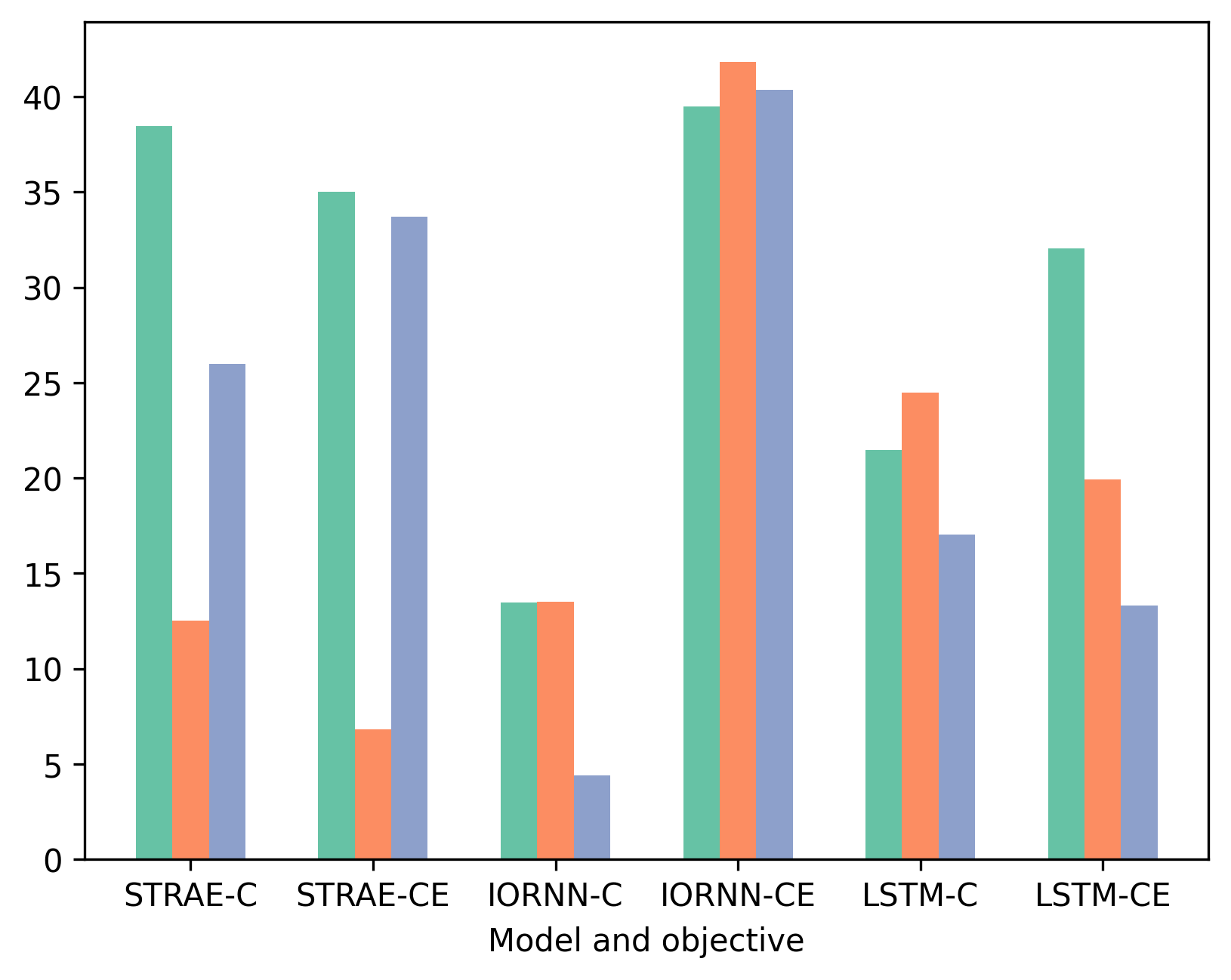
(b) Lexical Semantics

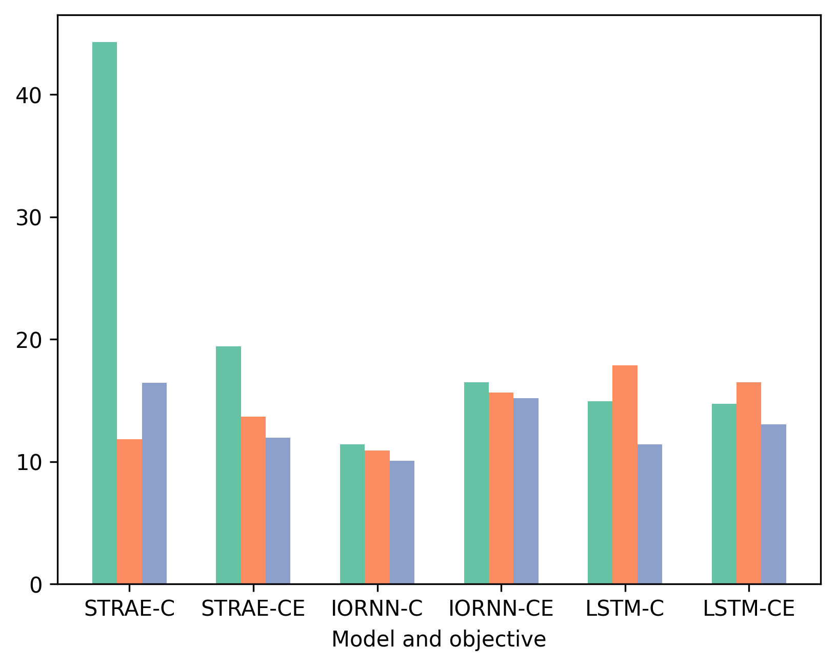
(c) Sentence Level Semantics

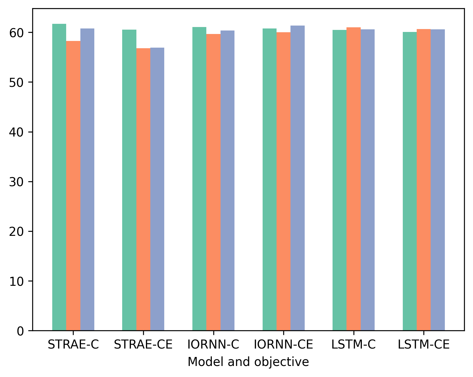
(d) Classification

Figure 3: Average performance for models on different task areas by structure type, higher is better.

Performance Across Input Structures

We also evaluate how dependent the performance of each model is on input structure. We compare the performance of each model between constituency parses, right-branching and balanced binary trees as input. Plots of these results are in Fig. 3, and the full tables can be seen in Appendix D. StrAE is dependent on input structure for performance, particularly when using the contrastive objective, though this still holds true across all task areas even for cross entropy. On the other hand, the baseline models are not, though this varies in degree. IORNN trained with cross entropy actually performs best with right-branching structure, though this is skewed by word level performance. Conversely, the LSTM appears to discriminate, but this is solely due to word level results and does not extend to other areas of evaluation.

Summary

StrAE is tasked with taking a sequence and compressing it into a single representation through ordered merges as dictated by the input tree. Each non-leaf node acts as a compression bottleneck. As a result, the contribution of each input token to the final root representation is directly dependent on the merge order. This makes StrAE structure sensitive. When coupled with contrastive loss, StrAE must learn embeddings such that similarity is dependent on how sequences compose. This is because the objective is now over all nodes, and all non-leaf node embeddings are defined by merge order. Secondly, it requires that the merge order have some degree of consistency to enable reconstruction, something which purely right-branching and balanced binary trees do not provide. It is the combination of strict compositional bottlenecking and the contrastive objective that enables StrAE to learn effective multi-level representations and serve as a probe for the utility of structure, unlike the tree structured baselines.

5 Comparison to Unstructured Baselines

Here, we compare StrAE to a series of baselines that are not provided any form of parse tree as input. The aim is to evaluate the usefulness of explicit structure against other inductive biases. We also introduce a variant of StrAE called Self-StrAE that is not provided structure as input but must learn its own mode of composition. It serves as a measure of the utility of an explicit compositional bottleneck.

Figure 4: Self-StrAE composition. Red dotted arrows indicate cosine similarity between nodes.

Self-StrAE

Self-StrAE (Self-Structuring AutoEncoder) modifies the encoder so it uses greedy agglomerative clustering in order to decide which tokens to compose. Unlike StrAE where the order of compositions is defined by the input structure, in Self-StrAE this is dictated by the embeddings. Self-StrAE orders compositions according to cosine similarity between adjacent node embeddings in the frontier, merging the argmax at each step. Figure Fig. 4 shows this process. In the figure, the similarity between ‘ate’ and ‘doughnuts’ is greater than that of ‘ate’ to ‘Homer’, so the model first merges ‘ate doughnuts’ into a single embedding using the composition function. At the next step, the model merges ‘Homer’ and ‘ate doughnuts’ into a single embedding and arrives at the root. The algorithm is provided in Appendix B.

We save the merge history in an adjacency matrix so that by the time the encoder reaches the root node, the adjacency matrix represents the whole tree over the input sequence. We then convert the adjacency matrix into a DGL graph, and pass that as input to the decoder. The decoder operates exactly the same as in vanilla StrAE, only that in this case the input graph is defined by the encoder’s merge history as opposed to, e.g., a syntactic parser.

Table 4: Comparison to unstructured baselines. Higher is better. All tasks that use Spearman’s $\rho$ have the result * 100 and are marked with a †. Score represents the average across all tasks. All models were trained over five random seeds. Only results where there is no standard deviation overlap between model performance are bolded.

Model	Simlex †	Wordsim S †	Wordsim R †	STS 12 †	STS 16 †	STS B †	SICK R †	MRPC	RTE	Score
StrAE Syntactic	15.54 $\pm$ 0.25	56.1 $\pm$ 0.47	43.77 $\pm$ 1.01	34.59 $\pm$ 2.58	50.4 $\pm$ 0.97	41.83 $\pm$ 2.23	50.3 $\pm$ 0.88	67.24 $\pm$ 0.39	56.16 $\pm$ 1.59	46.21
Self-StrAE BPE	13.04 $\pm$ 0.07	48.19 $\pm$ 1.03	45.47 $\pm$ 0.83	34.42 $\pm$ 0.73	49.93 $\pm$ 0.38	36.68 $\pm$ 0.64	51 $\pm$ 0.3	68.91 $\pm$ 0.2	54.42 $\pm$ 0.49	44.67
Self-StrAE Word	18.21 $\pm$ 0.12	53.52 $\pm$ 0.39	48.76 $\pm$ 0.86	33.22 $\pm$ 0.38	49.91 $\pm$ 0.35	27.97 $\pm$ 0.2	52 $\pm$ 0.52	68.13 $\pm$ 0.1	54.53 $\pm$ 0.53	45.14
Fasttext	25.8 $\pm$ 0.16	50.8 $\pm$ 0.24	29.18 $\pm$ 0.22	4.35 $\pm$ 0.6	32.43 $\pm$ 0.1	16.93 $\pm$ 0.09	41.58 $\pm$ 0.05	69.1 $\pm$ 0.12	54.4 $\pm$ 0.67	36.06
Bi-LSTM Word	23.74 $\pm$ 1.17	61.94 $\pm$ 2.44	41.46 $\pm$ 1.73	11.18 $\pm$ 1.1	34.86 $\pm$ 0.86	13.46 $\pm$ 1.11	42.36 $\pm$ 0.19	68.95 $\pm$ 0.38	54.09 $\pm$ 0.95	39.12
Bi-LSTM BPE	12.88 $\pm$ 0.77	39.46 $\pm$ 2.17	32.22 $\pm$ 3.07	9.22 $\pm$ 0.87	33.78 $\pm$ 1.66	14.06 $\pm$ 2.01	40.36 $\pm$ 0.27	68.21 $\pm$ 0.41	53.9 $\pm$ 0.96	33.79
RoBERTa	9.92 $\pm$ 2.7	26.6 $\pm$ 6.71	6.2 $\pm$ 3.81	29.48 $\pm$ 3.28	50.88 $\pm$ 1.11	38.36 $\pm$ 1.9	49.58 $\pm$ 0.91	69.19 $\pm$ 0.27	54.86 $\pm$ 0.49	37.23

Baselines

We selected Fasttext Bojanowski et al. (2016), a Bi-LSTM Hochreiter and Schmidhuber (1997) and RoBERTa Liu et al. (2019) as baselines. Fasttext leverages distributional semantics and subword information to learn word embeddings, but only operates over a fixed window size. The Bi-LSTM allows us to measure the utility of sequential vs hierarchical information processing. Finally, RoBERTa serves as a suitable Transformer baseline, because it only utilises the MLM objective, rather using NSP as with BERT Devlin et al. (2019), and this has been shown to be more robust. Furthermore, it does not require additional data labelling, such as identifying which sentences follow each other, which provides greater parity with Self-StrAE and Fasttext as both models do not have such additional labels as input. For both models, we set the embedding dimensionality to 100 to match StrAE and set the number of attention heads in RoBERTa to 10 in order to match StrAE’s channels. We set the number of layers in RoBERTa to 6 as, in a data constrained setting there was no additional benefit observed with a greater number, and the parameter disparity between StrAE and RoBERTa is already substantial (see Table 5 for parameter counts for both the tree and unstructured baselines). The other hyperparameter details for all baselines can be found in Appendix A. To produce sentence embeddings we take the mean of the word embeddings with Fasttext and the mean of the final layer token representations for RoBERTa. To produce word embeddings for RoBERTa we follow the lessons from Vulic et al. (2020); Jawahar et al. (2019), which state that lexical information is contained in the lower layers. For cases where a word is broken into multiple subwords, we take the average of the embeddings from layers 0-2. Where a word is present in the vocabulary, we simply use its embedding, as there is no context to provide it with. In the case of the Bi-LSTM we produce sentence embeddings by passing the concatenated final hidden states for both directions through a learned linear layer in order to produce a single 100-dimensional embedding. We found this to lead to improved performance compared to simply using the concatenation. The same strategy is used to produce word embeddings in the case where it is broken into multiple subwords. We contrast these models with StrAE trained on constituency parses with contrastive loss, Self-StrAE trained on the word level using the same vocabulary as before, and finally Self-StrAE starting from the subword level. We take the vocabulary from the same BPE Sennrich et al. (2016) tokeniser used by RoBERTa (minus the special tokens) with a total size of 25000. We train Self-StrAE with the contrastive objective because this proved significantly more effective.

Table 5: Number of parameters for our models and baselines. Following convention we exclude the embedding matrix (and LM head if applicable) from the count.

Model	(Self-)StrAE	IORNN	Tree-LSTM	Bi-LSTM	RoBERTa
Params	430	40,400	260,600	181,800	3,950,232

10 Million Tokens

As shown in Table 4, while StrAE performs best overall, Self-StrAE is able to achieve comparable performance across both the word and sentence level. Fasttext performs best on Simlex, but this is likely to be for the same reasons as IORNN i.e., capturing similarity at the expense of relatedness. This is also indicated by its comparative lower Wordsim R performance. On both other lexical semantics tasks StrAE and Self-StrAE both outperform it. Fasttext also struggles on the sentence level. Similarly, the Bi-LSTM performs well on lexical semantics, but struggles at capturing higher levels. This is evidenced both by the STS results and lower lexical performance of the BPE Bi-LSTM compared with Self-StrAE. RoBERTa performs comparably to StrAE on STS, but struggles on the word level. This might simply be because Transformers aren’t designed to learn static lexical embeddings, but could also be the result of our data-constrained pre-training setting, as there was significant variability between seeds. Consequently, we conducted a final experiment using a significantly larger pre-training set to assess the impact of scale.

Table 6: WikiText-103 Results. Higher is better. All tasks that use Spearman’s $\rho$ have the result * 100 and are marked with a †. Score represents the average across all tasks. All models were trained over five random seeds. Only results where there is no standard deviation overlap between model performance are bolded.

Model	Simlex †	Wordsim S †	Wordsim R †	STS 12 †	STS 16 †	STS B †	SICK R †	MRPC	RTE	Score
RoBERTa	19.28 $\pm$ 1.02	46.38 $\pm$ 3.18	26.12 $\pm$ 3.09	35.38 $\pm$ 1.47	52.64 $\pm$ 1.11	39.74 $\pm$ 1.04	50.68 $\pm$ 0.43	69.74 $\pm$ 0.42	53.71 $\pm$ 0.5	43.76
Self-StrAE	13.41 $\pm$ 0.66	47.06 $\pm$ 0.61	42.53 $\pm$ 1.71	46.64 $\pm$ 0.23	52.08 $\pm$ 0.37	40.59 $\pm$ 0.83	51.94 $\pm$ 0.4	68.35 $\pm$ 0.46	55.87 $\pm$ 0.3	46.39

100 Million tokens

For this experiment, we turned to the WikiText-103 benchmark dataset Merity et al. (2016). WikiText-103 consists of 103 million tokens, with an average sequence length of 118. Each input sequence corresponds to an article rather than a sentence, as in our original dataset. We set the maximum sequence length to 512 and train a subword tokeniser on the training set with a maximum vocabulary of 25000. This vocabulary is used for both RoBERTa and Self-StrAE. As shown in Table 6, under this setting, RoBERTa improves significantly on the word level. RoBERTa also shows improvement on the sentence level, though these are less pronounced as the model was already performing well on these tasks. Surprisingly, Self-StrAE is able to achieve comparable (and in some cases better) performance than the RoBERTa model, despite having orders of magnitude fewer parameters. We can only attribute Self-StrAE’s performance to the inductive bias behind it: that the model must perform hierarchical compositions of its input sequence. Which we believe speaks strongly to its merits.

Summary

Comparison with the unstructured baselines shows that explicitly incorporating hierarchical compositions to be beneficial for multi-level representation learning. With Self-StrAE we show that these benefits do necessitate an external parser for preprocessing, and can largely be achieved through an inductive bias for explicit merging.

6 Related Work

Recursive Neural Networks: StrAE belongs to the class of recursive neural networks (RvNNs). First popularised by Socher et al. (2011, 2013), who employed RvNNs to perform fine-grained sentiment analysis, utilising tree structure to overcome the deficits of bag of words models. These early successes inspired the creation of successor frameworks like the IORNN Le and Zuidema (2014) and Tree-LSTM Tai et al. (2015) we used as baselines.
Learning Tree Structure: The induction of structure has long been a goal of NLP. Early pivotal work on corpus based induction was performed by Klein and Manning (2004); Petrov et al. (2006), and enabled the development of work on tree-structured models that followed. A recent prominent approach is the C-PCFG Kim et al. (2019).
Induction Through Representation Learning: DIORA and subsequently S-DIORA Drozdov et al. (2019, 2020) are models which induce structure using the IORNN. Instead of providing a fixed tree as input, they train by using dynamic programming over the set of all possible trees based on how well IORNN is able to reconstruct the input sequence. At test time, they use CKY to extract the highest scoring tree as the parse, which achieved SOTA on unsupervised consituency parsing. While these do learn representations, they solely utilise it to enable unsupervised parsing.
Learning Task Specific Tree Structures: Inspired by Socher et al. (2011) prior work has sought to learn trees for supervised tasks Yogatama et al. (2017); Maillard et al. (2017); Choi et al. (2017), under the assumption that a particular task requires its own form of composition. They achieved success, but all use the Tree-LSTM, which was shown to be largely structure agnostic in the supervised setting Shi et al. (2018); a finding we confirm in this work.
The Utility of Structure: Prior work has also sought to augment the Transformer architecture with tree structure. Wang et al. (2019b) modify self-attention so that it may only operate within constituents. Zanzotto et al. (2020) provide a module that represents the parse tree for an input and allows the Transformer to attend to it. Sartran et al. (2022) perform pre-training using linearised trees. In all cases, it was found that structure aided with language modelling perplexity and generalisation.
Structure and Representation Learning: This area, the focus of our paper, remains largely underexplored. Prior work has solely examined the word level, using dependency parses to define the context neighbourhood for a given word. The first work to do this was Levy and Goldberg (2014) and achieved promising results, however, they faced issues with vocabulary size becoming intractable. Vashishth et al. (2019) alleviated this issue through the use of GCNs Kipf and Welling (2016).

7 Discussion and Future Work

We establish two findings. Firstly, defining representation similarity through composition is useful, and secondly, asking a model to arrange its own composition is a powerful inductive bias. Neither of these findings are limited in their application to the architecture presented in this paper. The requirements are: an explicit merge operation and an objective that optimises representations across all levels. As long as these conditions are met, the findings are in theory applicable to any number of architectures. For future development, the natural next step is to examine what happens when we allow for a significantly more flexible models to dictate their own compositions. Transformers can be naturally adapted to incorporate such a bias, and we believe this holds considerable promise for future work, especially in light of recent findings that incorporating compression bottlenecks in Transformers is beneficial Nawrot et al. (2021, 2023). Extensions need not be limited to the Transformer architecture, either. Recurrent and recursive neural networks share many similar features, and given the recent resurgence of RNNs Orvieto et al. (2023); Peng et al. (2023) there may also be promise in extending research in this direction.

Limitations

The particular Self-StrAE presented in this paper is a considerably limited model. It is minimally parameterised (see Table 5), locally greedy and makes uncontextualised decisions about which nodes to merge. The mode of composition it learns is certain to be suboptimal as a result of this, and it speaks to the strength of the inductive bias that it is able to perform at all. The structure it learns certainly doesn’t resemble syntax as we understand it (example trees can be found in Appendix C), and neither did we expect it to. A significantly more flexible model would likely be required in this regard. Even then, it is possible that the form of composition a model learns with respect to its training objective may deviate substantially from our expectations of how compositional structure should look. Secondly, the aim of this paper is to conduct basic research into the benefits of composition and not to outperform the state of the art. We believe there is promise in pursuing further research that may eventually lead to improvements over SOTA, but we leave this to future work.

Ethics Statement

The aim of this paper is to examine whether explicitly incorporating hierarchical compositions can be beneficial. The eventual intended goal is to make machine learning models less resource- and data-intensive. We believe this can provide considerable benefits in making research more accessible.

Appendix A Training Data and Hyper-parameters

We trained each StrAE (and the tree baselines) model for 15 epochs (sufficient for convergence) using the Adam optimizer with a learning rate of 1e-3 for cross entropy and 1e-4 for contrastive loss, using a batch size of 128. We applied dropout of 0.2 on the embeddings and 0.1 on the composition and decomposition functions. The temperature hyper-parameter for the contrastive objective was set to 0.2 and the r value 0.1. These settings were obtained by a grid search over the values r= 1.0, 0.1, 0.01, batch size = 128, 256, 512, 768, $\tau$ = 0.2, 0.4, 0.6, 0.8 and learning rate 1e-3, 5e-4, and 1e-4. The Fasttext baseline was trained for 15 epochs with a learning rate of 1e-3, and a window size of 10. Self-StrAE was trained using the same hyperparameters as StrAE, except on Wikitext-103 where we lowered the learning rate to 5e-5 and increased $\tau$ to 0.6, and decreased r to 0.0001. RoBERTa was trained for 100 epochs, with a 10% of steps used for warmup, a learning rate of 5e-5 and a linear schedule. We used relative key-query positional embeddings. The Bi-LSTM was trained for 15 epochs with learning rate 1e-3, batch size 128 and dropout of 0.2 applied to the embeddings and output layer.

Appendix B Self-StrAE Algorithm

Algorithm 1 Self-StrAE Agglomerative Compose

0:  Node frontier $\{e_{n}\}_{n=1}^{N}$, composition ($\circ$)pairwise node similarity cSim$(e,e^{\prime})$

1:  $\mathcal{A}\leftarrow\{e_{n}\}_{n=1}^{N}$                 $\triangleright$ initialise frontier

2:  $\mathcal{T}\leftarrow\varnothing$                   $\triangleright$ initialise tree merges

3:  while $\lvert\mathcal{A}\rvert>1$ do

4:     $\displaystyle e_{i}^{\star},e_{i+1}^{\star}\leftarrow\operatorname*{arg\,max}_{e_{i},e_{i+1}\in\mathcal{A}}\textsc{cSim}(e_{i},e_{i+1})$            $\triangleright$ choose closest adjacent pair in $\mathcal{A}$

5:     $\mathcal{A}\leftarrow\mathcal{A}\setminus\{e_{i}^{\star},e_{i+1}^{\star}\}$    $\triangleright$ remove from frontier

6:     $e_{p}^{\star}=\circ(e_{i}^{\star},e_{i+1}^{\star})$      $\triangleright$ compute composition

7:     $\mathcal{A}\leftarrow\mathcal{A}\cup_{i}\{e_{p}^{\star}\}$        $\triangleright$ insert into frontier at $i$

8:     $\mathcal{T}\leftarrow\mathcal{T}\cup\{(i,i+1)\}$    $\triangleright$ record merge location

9:  return  Merge order $\mathcal{T}$

Appendix C Tree Statistics and Examples

Self-StrAE learns trees which are not purely right-branching, balanced binary, or purely random. We parse our development split using Self-StrAE BPE models pre-trained on the 10M corpus. The split itself consists of 40k sentences with an average length of 23.58. The trees from Self-StrAE have an average depth of 9, compared with 23 (rounding up for simplicity) for right-branching trees, and 5 for balanced binary trees. Self-StrAE trees exhibit a slight preference for right-branching, with each non-leaf node on average having fewer left than right successors 60% of the time.

However, the best way to get a sense for the kind of structures the model learns is by looking at examples shown on the following pages. Looking at the examples in Fig. 5 and Fig. 6 the model has learned some sensible pattens. For example, it has learned to segment sentences with embedded clauses or conjunctions into their constituent parts (e.g. Fig. 5a,e,g and Fig. 6a). However, the trees frequently exhibit attachment errors that we hypothesize are the result of structure being determined by co-occurrence frequency. For example, in Fig. 6a the model merges [will be] as its own constituent rather than the correct parse of [will [be cancelled]]. Which is likely because “will” and “be” co-occur much more frequently than any instance of “be” + passive form of a given verb. Similar behaviour can be found all throughout the examples in Fig. 5 and Fig. 6. Given the simplicity of the model it is unsurprising that Self-StrAE is unable to learn deeper rules, however, it would be interesting to determine to what extent this is also a function of the data it is trained on. Recent work has shown that transcribed child directed speech leads transformer models to learn grammar more efficiently Huebner et al. (2021); Mueller and Linzen (2023). Transcribed CDS is far less regular than Wikipedia and may cause the model to avoid simpler heuristics like bigram frequency.

Finally, there are cases where the model seems to be learning totally implausible structures. We are yet to determine the root cause of this, but include examples in Fig. 7 for the sake of transparency.

(a) Self-StrAE

(b) CoreNLP

(c) Self-StrAE

(d) CoreNLP

(e) Self-StrAE

(f) CoreNLP

(g) Self-StrAE

(h) CoreNLP

Figure 5: Comparison of trees: Self-StrAE vs. CoreNLP

(a) Self-StrAE

(b) CoreNLP

(c) Self-StrAE

(d) CoreNLP

(e) Self-StrAE

(f) CoreNLP

(g) Self-StrAE

(h) CoreNLP

Figure 6: Comparison of trees: Self-StrAE vs. CoreNLP

Figure 7: Incomprehensible Cases

Appendix D Performance by Structure Type

We show in Table 7 a comparison of performance for different structure types and objectives used in this work. As discussed earlier, the objectives used here are contrastive (C) and standard cross-entropy (CE), and the structure types explored are the syntactic, purely right branching (RB) and the balanced binary (BB) trees.

Table 7: Comparison Across Structure Type

Model	Simlex	Wordsim S	Wordsim R	STS 12	STS 16	STS B	SICK R	MRPC	RTE
StrAE Syntactic C	15.54 $\pm$ 0.25	56.1 $\pm$ 0.47	43.77 $\pm$ 1.01	34.59 $\pm$ 2.58	50.4 $\pm$ 0.97	41.83 $\pm$ 2.23	50.3 $\pm$ 0.88	67.24 $\pm$ 0.39	56.16 $\pm$ 1.59
StrAE Syntactic CE	17.57 $\pm$ 1.08	50.72 $\pm$ 2.97	36.73 $\pm$ 6.19	5.02 $\pm$ 1.1	25.86 $\pm$ 1.03	7.76 $\pm$ 0.95	39.06 $\pm$ 1.51	67.48 $\pm$ 0.3	53.6 $\pm$ 0.46
IORNN Syntactic C	1.9 $\pm$ 0.25	27.29 $\pm$ 0.57	11.29 $\pm$ 0.5	-4.2 $\pm$ 0.97	17.47 $\pm$ 1.14	1.87 $\pm$ 0.55	30.48 $\pm$ 0.55	67.08 $\pm$ 0.16	55 $\pm$ 1.44
IORNN Syntactic CE	24.36 $\pm$ 0.6	57.53 $\pm$ 1.59	36.55 $\pm$ 1.78	-0.17 $\pm$ 0.92	22.68 $\pm$ 0.98	5.04 $\pm$ 0.55	38.41 $\pm$ 0.63	67.24 $\pm$ 0.63	54.28 $\pm$ 0.55
LSTM Syntactic C	6.45 $\pm$ 0.4	37.39 $\pm$ 1.2	20.6 $\pm$ 1.49	-1.34 $\pm$ 1.33	23.95 $\pm$ 0.45	4.25 $\pm$ 1.11	32.9 $\pm$ 0.55	68.16 $\pm$ 0.32	52.76 $\pm$ 1.09
LSTM Syntactic CE	14.23 $\pm$ 2.01	48.7 $\pm$ 3.22	33.24 $\pm$ 3.02	-1.66 $\pm$ 1.29	19.38 $\pm$ 1.21	6.7 $\pm$ 1.04	34.55 $\pm$ 1.15	68 $\pm$ 0.0	52.2 $\pm$ 1.98
StrAE RB C	4.6 $\pm$ 2.5	19.6 $\pm$ 9.0	13.4 $\pm$ 9.2	3.7 $\pm$ 4.0	17.9 $\pm$ 10.9	3.11 $\pm$ 5.36	22.65 $\pm$ 2.88	66.32 $\pm$ 0.44	50.2 $\pm$ 1.77
StrAE RB CE	7.76 $\pm$ 2.23	9.79 $\pm$ 4.3	2.85 $\pm$ 7.76	9.94 $\pm$ 1.86	14.17 $\pm$ 1.95	3.87 $\pm$ 2.47	26.77 $\pm$ 1.41	62.24 $\pm$ 9.71	51.4 $\pm$ 1.48
IORNN RB C	3.66 $\pm$ 0.21	28.24 $\pm$ 0.75	8.7$\pm$ 3.73	2.92 $\pm$ 1.31	18.5 $\pm$ 0.95	-2.47 $\pm$ 1.23	24.6 $\pm$ 1.67	67.15 $\pm$ 0.26	52.2 $\pm$ 0.88
IORNN RB CE	23.27 $\pm$ 0.416	61.79 $\pm$1.72	40.42 $\pm$ 3.02	8.85 $\pm$0.75	24.79 $\pm$ 0.2	3.38 $\pm$0.49	25.53 $\pm$ 0.79	67 $\pm$ 0.17	53 $\pm$ 0.54
LSTM RB C	9.58 $\pm$ 0.76	40.97 $\pm$ 0.94	22.87 $\pm$ 0.4	6.96 $\pm$ 0.77	32.17 $\pm$ 0.43	2.76 $\pm$ 0.31	29.65 $\pm$ 0.31	68.36 $\pm$ 0.39	53.6 $\pm$ 0.75
LSTM RB CE	8.69 $\pm$ 2.21	31.62 $\pm$ 3.79	19.43 $\pm$ 5.84	12.67 $\pm$ 2.85	18.65 $\pm$ 3.06	5.87 $\pm$ 3.51	28.67 $\pm$ 0.53	68.16 $\pm$ 0.32	53.12 $\pm$ 1.31
StrAE BB C	1.0 $\pm$ 4.9	43.4 $\pm$ 16.9	33.6 $\pm$ 12.6	16.6 $\pm$ 3.0	16 $\pm$ 4.6	9 $\pm$ 3.0	24.18 $\pm$ 0.32	68 $\pm$ 0.0	53.5 $\pm$ 0.0
StrAE BB CE	13.59 $\pm$ 2.15	52.4 $\pm$ 1.7	35.08 $\pm$ 2.42	3.46 $\pm$ 1.86	19.66 $\pm$ 1.34	-0.37 $\pm$ 1.75	24.99 $\pm$ 0.43	61.28 $\pm$ 0.57	52.56 $\pm$ 0.84
IORNN BB C	2.2 $\pm$ 0.85	8.39 $\pm$2.85	2.64$\pm$ 1.86	0.77 $\pm$ 0.55	10.9 $\pm$ 0.09	7.67 $\pm$ 0.57	20.88 $\pm$ 0.37	67.48 $\pm$ 0.35	53.24 $\pm$ 0.43
IORNN BB CE	19.02 $\pm$ 0.48	57.14 $\pm$ 0.91	44.92 $\pm$ 0.98	9.46 $\pm$ 0.58	18.11$\pm$ 0.81	8.86 $\pm$0.91	24.3 $\pm$ 0.93	67.4$\pm$ 0.36	55.36 $\pm$ 1.06
LSTM BB C	4.28 $\pm$ 0.65	28.17 $\pm$ 1.32	18.72 $\pm$ 1.91	10.51 $\pm$ 0.54	10.75 $\pm$ 0.44	1.05 $\pm$ 0.18	23.32 $\pm$ 0.33	68.0 $\pm$ 0.00	53.00$\pm$ 0.70
LSTM BB CE	4.67 $\pm$ 2.78	21.21 $\pm$ 6.27	14.04 $\pm$ 4.78	8.13 $\pm$ 2.18	12.99 $\pm$ 1.77	9.90 $\pm$ 9.90	21.15$\pm$ 1.43	68.0 $\pm$ 0.00	53.20 $\pm$ 0.81

References

- Agirre et al. (2009) Eneko Agirre, Enrique Alfonseca, Keith Hall, Jana Kravalova, Marius Paşca, and Aitor Soroa. 2009. A study on similarity and relatedness using distributional and WordNet-based approaches. In North American Chapter of the Association for Computational Linguistics (NAACL), pages 19–27.
- Agirre et al. (2016) Eneko Agirre, Carmen Banea, Daniel Cer, Mona Diab, Aitor Gonzalez-Agirre, Rada Mihalcea, German Rigau, and Janyce Wiebe. 2016. SemEval-2016 task 1: Semantic textual similarity, monolingual and cross-lingual evaluation. In Proceedings of the 10th International Workshop on Semantic Evaluation (SemEval-2016), pages 497–511, San Diego, California. Association for Computational Linguistics.
- Agirre et al. (2012) Eneko Agirre, Mona Diab, Daniel Cer, and Aitor Gonzalez-Agirre. 2012. Semeval-2012 task 6: A pilot on semantic textual similarity. In Proceedings of the First Joint Conference on Lexical and Computational Semantics - Volume 1: Proceedings of the Main Conference and the Shared Task, and Volume 2: Proceedings of the Sixth International Workshop on Semantic Evaluation, SemEval ’12, page 385–393, USA. Association for Computational Linguistics.
- Bird et al. (2009) Steven Bird, Ewan Klein, and Edward Loper. 2009. Natural language processing with Python: analyzing text with the natural language toolkit.
- Bojanowski et al. (2016) Piotr Bojanowski, Edouard Grave, Armand Joulin, and Tomás Mikolov. 2016. Enriching word vectors with subword information. CoRR, abs/1607.04606.
- Cer et al. (2017) Daniel Cer, Mona Diab, Eneko Agirre, Iñigo Lopez-Gazpio, and Lucia Specia. 2017. SemEval-2017 task 1: Semantic textual similarity multilingual and crosslingual focused evaluation. In Workshop on Semantic Evaluation (SemEval), pages 1–14.
- Chen et al. (2020) Ting Chen, Simon Kornblith, Mohammad Norouzi, and Geoffrey E. Hinton. 2020. A simple framework for contrastive learning of visual representations. In International Conference on Learning Representations (ICLR), volume 119, pages 1597–1607.
- Choi et al. (2017) Jihun Choi, Kang Min Yoo, and Sang-goo Lee. 2017. Learning to compose task-specific tree structures.
- Chomsky (1956) N. Chomsky. 1956. Three models for the description of language. IRE Transactions on Information Theory, 2(3):113–124.
- Crain and Nakayama (1987) Stephen Crain and Mineharu Nakayama. 1987. Structure dependence in grammar formation. Language, 63(3):522–543.
- de Marneffe et al. (2006) Marie-Catherine de Marneffe, Bill MacCartney, and Christopher D. Manning. 2006. Generating typed dependency parses from phrase structure parses. In Proceedings of the Fifth International Conference on Language Resources and Evaluation (LREC’06), Genoa, Italy. European Language Resources Association (ELRA).
- Devlin et al. (2019) Jacob Devlin, Ming-Wei Chang, Kenton Lee, and Kristina Toutanova. 2019. BERT: Pre-training of deep bidirectional transformers for language understanding. In North American Chapter of the Association for Computational Linguistics (NAACL), pages 4171–4186.
- Dong and Lapata (2016) Li Dong and Mirella Lapata. 2016. Language to logical form with neural attention. CoRR, abs/1601.01280.
- Drozdov et al. (2020) Andrew Drozdov, Subendhu Rongali, Yi-Pei Chen, Tim O’Gorman, Mohit Iyyer, and Andrew McCallum. 2020. Unsupervised parsing with S-DIORA: Single tree encoding for deep inside-outside recursive autoencoders. In Proceedings of the 2020 Conference on Empirical Methods in Natural Language Processing (EMNLP), pages 4832–4845, Online. Association for Computational Linguistics.
- Drozdov et al. (2019) Andrew Drozdov, Patrick Verga, Mohit Yadav, Mohit Iyyer, and Andrew McCallum. 2019. Unsupervised latent tree induction with deep inside-outside recursive autoencoders. CoRR, abs/1904.02142.
- Hill et al. (2015) Felix Hill, Roi Reichart, and Anna Korhonen. 2015. SimLex-999: Evaluating semantic models with (genuine) similarity estimation. Computational Linguistics, 41(4):665–695.
- Hochreiter and Schmidhuber (1997) Sepp Hochreiter and Jürgen Schmidhuber. 1997. Long short-term memory. Neural computation, 9:1735–80.
- Huebner et al. (2021) Philip A. Huebner, Elior Sulem, Fisher Cynthia, and Dan Roth. 2021. BabyBERTa: Learning more grammar with small-scale child-directed language. In Proceedings of the 25th Conference on Computational Natural Language Learning, pages 624–646, Online. Association for Computational Linguistics.
- Jawahar et al. (2019) Ganesh Jawahar, Benoît Sagot, and Djamé Seddah. 2019. What does BERT learn about the structure of language? In Association for Computational Linguistics (ACL), pages 3651–3657.
- Kim et al. (2020) Taeuk Kim, Jihun Choi, Daniel Edmiston, and Sang-goo Lee. 2020. Are pre-trained language models aware of phrases? simple but strong baselines for grammar induction. In International Conference on Learning Representations (ICLR).
- Kim et al. (2019) Yoon Kim, Chris Dyer, and Alexander Rush. 2019. Compound probabilistic context-free grammars for grammar induction. In Proceedings of the 57th Annual Meeting of the Association for Computational Linguistics, pages 2369–2385, Florence, Italy. Association for Computational Linguistics.
- Kipf and Welling (2016) Thomas N. Kipf and Max Welling. 2016. Semi-supervised classification with graph convolutional networks. CoRR, abs/1609.02907.
- Klein and Manning (2004) Dan Klein and Christopher Manning. 2004. Corpus-based induction of syntactic structure: Models of dependency and constituency. In Proceedings of the 42nd Annual Meeting of the Association for Computational Linguistics (ACL-04), pages 478–485, Barcelona, Spain.
- Lake et al. (2017) Brenden M. Lake, Tomer D. Ullman, Joshua B. Tenenbaum, and Samuel J. Gershman. 2017. Building machines that learn and think like people. Behavioral and Brain Sciences, 40:e253.
- Le and Zuidema (2014) Phong Le and Willem Zuidema. 2014. Inside-outside semantics: A framework for neural models of semantic composition. In NIPS 2014 Workshop on Deep Learning and Representation Learning.
- Levy and Goldberg (2014) Omer Levy and Yoav Goldberg. 2014. Dependency-based word embeddings. In Association for Computational Linguistics (ACL)(Volume 2: Short Papers), pages 302–308.
- Liu et al. (2019) Yinhan Liu, Myle Ott, Naman Goyal, Jingfei Du, Mandar Joshi, Danqi Chen, Omer Levy, Mike Lewis, Luke Zettlemoyer, and Veselin Stoyanov. 2019. Roberta: A robustly optimized BERT pretraining approach. CoRR, abs/1907.11692.
- Maillard et al. (2017) Jean Maillard, Stephen Clark, and Dani Yogatama. 2017. Jointly learning sentence embeddings and syntax with unsupervised tree-lstms. CoRR, abs/1705.09189.
- Manning et al. (2014) Christopher Manning, Mihai Surdeanu, John Bauer, Jenny Finkel, Steven Bethard, and David McClosky. 2014. The Stanford CoreNLP natural language processing toolkit. In Association for Computational Linguistics (ACL): System Demonstrations, pages 55–60.
- Marelli et al. (2014) Marco Marelli, Stefano Menini, Marco Baroni, Luisa Bentivogli, Raffaella Bernardi, and Roberto Zamparelli. 2014. A SICK cure for the evaluation of compositional distributional semantic models. In Proceedings of the Ninth International Conference on Language Resources and Evaluation (LREC’14), pages 216–223, Reykjavik, Iceland. European Language Resources Association (ELRA).
- Merity et al. (2016) Stephen Merity, Caiming Xiong, James Bradbury, and Richard Socher. 2016. Pointer sentinel mixture models. CoRR, abs/1609.07843.
- Mueller and Linzen (2023) Aaron Mueller and Tal Linzen. 2023. How to plant trees in language models: Data and architectural effects on the emergence of syntactic inductive biases. ArXiv, abs/2305.19905.
- Murty et al. (2022) Shikhar Murty, Pratyusha Sharma, Jacob Andreas, and Christopher D. Manning. 2022. Characterizing intrinsic compositionality in transformers with tree projections.
- Nawrot et al. (2023) Piotr Nawrot, Jan Chorowski, Adrian Łańcucki, and Edoardo M. Ponti. 2023. Efficient transformers with dynamic token pooling.
- Nawrot et al. (2021) Piotr Nawrot, Szymon Tworkowski, Michal Tyrolski, Lukasz Kaiser, Yuhuai Wu, Christian Szegedy, and Henryk Michalewski. 2021. Hierarchical transformers are more efficient language models. CoRR, abs/2110.13711.
- Orvieto et al. (2023) Antonio Orvieto, Samuel L Smith, Albert Gu, Anushan Fernando, Caglar Gulcehre, Razvan Pascanu, and Soham De. 2023. Resurrecting recurrent neural networks for long sequences.
- Pallier et al. (2011) Christophe Pallier, Anne-Dominique Devauchelle, and Stanislas Dehaene. 2011. Cortical representation of the constituent structure of sentences. Proceedings of the National Academy of Sciences, 108(6):2522–2527.
- Peng et al. (2023) Bo Peng, Eric Alcaide, Quentin Anthony, Alon Albalak, Samuel Arcadinho, Huanqi Cao, Xin Cheng, Michael Chung, Matteo Grella, Kranthi Kiran GV, Xuzheng He, Haowen Hou, Przemyslaw Kazienko, Jan Kocon, Jiaming Kong, Bartlomiej Koptyra, Hayden Lau, Krishna Sri Ipsit Mantri, Ferdinand Mom, Atsushi Saito, Xiangru Tang, Bolun Wang, Johan S. Wind, Stansilaw Wozniak, Ruichong Zhang, Zhenyuan Zhang, Qihang Zhao, Peng Zhou, Jian Zhu, and Rui-Jie Zhu. 2023. Rwkv: Reinventing rnns for the transformer era.
- Petrov et al. (2006) Slav Petrov, Leon Barrett, Romain Thibaux, and Dan Klein. 2006. Learning accurate, compact, and interpretable tree annotation. In Proceedings of the 21st International Conference on Computational Linguistics and 44th Annual Meeting of the Association for Computational Linguistics, pages 433–440, Sydney, Australia. Association for Computational Linguistics.
- Radford et al. (2021) Alec Radford, Jong Wook Kim, Chris Hallacy, Aditya Ramesh, Gabriel Goh, Sandhini Agarwal, Girish Sastry, Amanda Askell, Pamela Mishkin, Jack Clark, et al. 2021. Learning transferable visual models from natural language supervision. In International Conference on Machine Learning (ICML), pages 8748–8763. PMLR.
- Sartran et al. (2022) Laurent Sartran, Samuel Barrett, Adhiguna Kuncoro, Miloš Stanojević, Phil Blunsom, and Chris Dyer. 2022. Transformer grammars: Augmenting transformer language models with syntactic inductive biases at scale. arXiv preprint arXiv:2203.00633.
- Sennrich et al. (2016) Rico Sennrich, Barry Haddow, and Alexandra Birch. 2016. Neural machine translation of rare words with subword units. In Association for Computational Linguistics (ACL), pages 1715–1725.
- Shi et al. (2018) Haoyue Shi, Hao Zhou, Jiaze Chen, and Lei Li. 2018. On tree-based neural sentence modeling. In Empirical Methods in Natural Language Processing (EMNLP), pages 4631–4641.
- Shi et al. (2020) Yuge Shi, Brooks Paige, Philip Torr, and N. Siddharth. 2020. Relating by contrasting: A data-efficient framework for multimodal generative models. In International Conference on Learning Representations (ICLR).
- Socher et al. (2011) Richard Socher, Jeffrey Pennington, Eric H. Huang, Andrew Y. Ng, and Christopher D. Manning. 2011. Semi-supervised recursive autoencoders for predicting sentiment distributions. In Empirical Methods in Natural Language Processing (EMNLP), pages 151–161.
- Socher et al. (2013) Richard Socher, Alex Perelygin, Jean Wu, Jason Chuang, Christopher D. Manning, Andrew Ng, and Christopher Potts. 2013. Recursive deep models for semantic compositionality over a sentiment treebank. In Empirical Methods in Natural Language Processing (EMNLP), pages 1631–1642.
- Tai et al. (2015) Kai Sheng Tai, Richard Socher, and Christopher D. Manning. 2015. Improved semantic representations from tree-structured long short-term memory networks. In Association for Computational Linguistics (ACL), pages 1556–1566.
- Vashishth et al. (2019) Shikhar Vashishth, Manik Bhandari, Prateek Yadav, Piyush Rai, Chiranjib Bhattacharyya, and Partha Talukdar. 2019. Incorporating syntactic and semantic information in word embeddings using graph convolutional networks. In Association for Computational Linguistics (ACL), pages 3308–3318.
- Vaswani et al. (2017) Ashish Vaswani, Noam Shazeer, Niki Parmar, Jakob Uszkoreit, Llion Jones, Aidan N. Gomez, Lukasz Kaiser, and Illia Polosukhin. 2017. Attention is all you need. In Advances in Neural Information Processing Systems (NeuRIPS), pages 5998–6008.
- Vulic et al. (2020) Ivan Vulic, Edoardo Maria Ponti, Robert Litschko, Goran Glavas, and Anna Korhonen. 2020. Probing pretrained language models for lexical semantics. CoRR, abs/2010.05731.
- Wang et al. (2019a) Alex Wang, Amanpreet Singh, Julian Michael, Felix Hill, Omer Levy, and Samuel R. Bowman. 2019a. GLUE: A multi-task benchmark and analysis platform for natural language understanding. In International Conference on Learning Representations (ICLR).
- Wang et al. (2020) Minjie Wang, Da Zheng, Zihao Ye, Quan Gan, Mufei Li, Xiang Song, Jinjing Zhou, Chao Ma, Lingfan Yu, Yu Gai, Tianjun Xiao, Tong He, George Karypis, Jinyang Li, and Zheng Zhang. 2020. Deep graph library: A graph-centric, highly-performant package for graph neural networks.
- Wang and Isola (2020) Tongzhou Wang and Phillip Isola. 2020. Understanding contrastive representation learning through alignment and uniformity on the hypersphere. CoRR, abs/2005.10242.
- Wang et al. (2019b) Yaushian Wang, Hung-Yi Lee, and Yun-Nung Chen. 2019b. Tree transformer: Integrating tree structures into self-attention. In Empirical Methods in Natural Language Processing and International Joint Conference on Natural Language Processing (EMNLP-IJCNLP), pages 1061–1070.
- Xiao et al. (2022) Dongling Xiao, Linzheng Chai, Qian-Wen Zhang, Zhao Yan, Zhoujun Li, and Yunbo Cao. 2022. Cqr-sql: Conversational question reformulation enhanced context-dependent text-to-sql parsers.
- Yogatama et al. (2017) Dani Yogatama, Phil Blunsom, Chris Dyer, Edward Grefenstette, and Wang Ling. 2017. Learning to compose words into sentences with reinforcement learning. In International Conference on Learning Representations (ICLR).
- Zanzotto et al. (2020) Fabio Massimo Zanzotto, Andrea Santilli, Leonardo Ranaldi, Dario Onorati, Pierfrancesco Tommasino, and Francesca Fallucchi. 2020. KERMIT: Complementing transformer architectures with encoders of explicit syntactic interpretations. In Empirical Methods in Natural Language Processing (EMNLP), pages 256–267.