Improving Implicit Feedback-Based Recommendation
through Multi-Behavior Alignment

Abstract.

Recommender systems that learn from implicit feedback often use large volumes of a single type of implicit user feedback, such as clicks, to enhance the prediction of sparse target behavior such as purchases. Using multiple types of implicit user feedback for such target behavior prediction purposes is still an open question. Existing studies that attempted to learn from multiple types of user behavior often fail to: (i) learn universal and accurate user preferences from different behavioral data distributions, and (ii) overcome the noise and bias in observed implicit user feedback.

To address the above problems, we propose multi-behavior alignment (MBA), a novel recommendation framework that learns from implicit feedback by using multiple types of behavioral data. We conjecture that multiple types of behavior from the same user (e.g., clicks and purchases) should reflect similar preferences of that user. To this end, we regard the underlying universal user preferences as a latent variable. The variable is inferred by maximizing the likelihood of multiple observed behavioral data distributions and, at the same time, minimizing the Kullback–Leibler divergence (KL-divergence) between user models learned from auxiliary behavior (such as clicks or views) and the target behavior separately. MBA infers universal user preferences from multi-behavior data and performs data denoising to enable effective knowledge transfer. We conduct experiments on three datasets, including a dataset collected from an operational e-commerce platform. Empirical results demonstrate the effectiveness of our proposed method in utilizing multiple types of behavioral data to enhance the prediction of the target behavior.

1. Introduction

Recommender systems aim to infer user preferences from observed user-item interactions and recommend items that match those preferences. Many operational recommender systems are trained from implicit user feedback (Gu et al., 2020; Huang et al., 2019). Recommender systems that learn from implicit user feedback are typically trained on a single type of implicit user behavior, such as clicks. However, in real-world scenarios, multiple types of user behavior are logged when a user interacts with a recommender system. For example, users may click, add to a cart, and purchase items on an e-commerce platform (Tsagkias et al., 2020). Simply learning recommenders from a single type of behavioral data such as clicks can lead to a misunderstanding of a user’s real user preferences since the click data is noisy and can easily be corrupted due to bias (Chen et al., 2020a), and thus lead to suboptimal target behavior (e.g., purchases) predictions. Meanwhile, only considering purchase data tends to lead to severe cold-start problems (Pan et al., 2019; Xie et al., 2020; Zhu et al., 2021) and data sparsity problems (Pan et al., 2010; Ma et al., 2022b).

Using multiple types of behavioral data. How can we use multiple types of auxiliary behavioral data (such as clicks) to enhance the prediction of sparse target user behavior (such as purchases) and thereby improve recommendation performance? Some prior work (Gao et al., 2019; Chen et al., 2020b) has used multi-task learning to train recommender systems on both target behavior and multiple types of auxiliary behavior. Building on recent advances in graph neural networks, Jin et al. (2020) encode target behavior and multiple types of auxiliary behavior into a heterogeneous graph and perform convolution operations on the constructed graph for recommendation. In addition, recent research tries to integrate the micro-behavior of user-item interactions into representation learning in the sequential and session-based recommendation (Zhou et al., 2018; Meng et al., 2020; Yuan et al., 2022). These publications focus on mining user preferences from user-item interactions, which is different from our task of predicting target behavior from multiple types of user behavior.

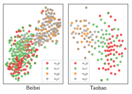
Figure 1. Distributions of items interacted with by two users in the Beibei and Taobao datasets (described in §4.2). Item representations are obtained by a matrix factorization model trained on the purchase behavior data. $u_{i}c$ ($u_{i}p$) represents the distribution of items clicked (purchased) by user $u_{i}$.

Limitations of current approaches. Prior work on using multiple types of behavioral data to improve the prediction of the target behavior in a recommendation setting has two main limitations.

The first limitation concerns the gap between data distributions of different types of behavior. This gap impacts the learning of universal and effective user preferences. For example, users may have clicked on but not purchased items, resulting in different positive and negative instance distributions across auxiliary and target behaviors. Existing work typically learns separate user preferences for different types of behavior and then combines those preferences to obtain an aggregate user representation. We argue that: (i) user preferences learned separately based on different types of behavior may not consistently lead to the true user preferences, and (ii) multiple types of user behavior should reflect similar user preferences; in other words, there should be an underlying universal set of user preferences under different types of behavior of the same user.

The second limitation concerns the presence of noise and bias in auxiliary behavioral data, which impacts knowledge extraction and transfer. A basic assumption of recommendations based on implicit feedback is that observed interactions between users and items reflect positive user preferences, while unobserved interactions are considered negative training instances. However, this assumption seldom holds in reality. A click may be triggered by popularity bias (Chen et al., 2020a), which does not reflect a positive preference. And an unobserved interaction may be attributed to a lack of exposure (Chen et al., 2021b). Hence, simply incorporating noisy or biased behavioral data may lead to sub-optimal recommendation performance.

Motivation. Our assumption is that multiple types of behavior from the same user (e.g., clicks and purchases) should reflect similar preferences of that user. To illustrate this assumption, consider Figure 1, which shows distributions of items that two users ($u_{1}$ and $u_{2}$) interacted with (clicks $c$ and purchases $p$), in the Beibei and Taobao datasets (described in Section 4.2 below). For both users, the items they clicked or purchased are relatively close. These observations motivate our hypothesis that multiple types of user behavior reflect similar user preferences, which is vital to improve the recommendation performance further.

Proposed method. To address the problem of learning from multiple types of auxiliary behavioral data and improve the prediction of the target behavior (and hence recommendation performance), we propose a training framework called multi-behavior alignment (MBA). MBA aligns user preferences learned from different types of behavior. The key assumption behind MBA is that multiple types of behavior from the same user reflect similar underlying user preferences.

To address the data distribution limitation mentioned above, we utilize KL-divergence to measure the discrepancy between user models learned from multiple types of auxiliary behavior and target behavior, and then conduct knowledge transfer by minimizing this discrepancy to improve the recommendation performance.

For the second limitation mentioned above (concerning noise and bias in behavioral data), MBA regards the underlying universal user preferences as a latent variable. The variable is then inferred by maximizing the likelihood of multiple types of observed behavioral data while minimizing the discrepancy between models trained on different types of behavioral data. In this manner, MBA denoises multiple types of behavioral data and enables more effective knowledge transfer across multiple types of user behavior.

To demonstrate the effectiveness of the proposed method, we conduct extensive experiments on two open benchmark datasets and one dataset collected from an operational e-commerce platform. Experimental results show that the proposed MBA framework outperforms related state-of-the-art baselines.

Main contributions. Our main contributions are as follows:

• We argue that multiple types of auxiliary and target behavior should reflect similar user preferences, and we propose to infer the true user preferences from multiple types of behavioral data.

• We propose a learning framework MBA to jointly perform data denoising and knowledge transfer across multiple types of behavioral data to enhance target behavior prediction and hence improve the recommendation performance.

• We conduct experiments on three datasets to demonstrate the effectiveness of the MBA method. One of these datasets is collected from an operational e-commerce platform, and includes clicks and purchase behavior data. Experimental results show state-of-the-art recommendation performance of the proposed MBA method.

2. Related work

We review prior work on multi-behavior recommendation and on denoising methods for recommendation from implicit feedback.

2.1. Multi-behavior recommendation

Unlike conventional implicit feedback recommendation models (Koren et al., 2009; He et al., 2020), which train a recommender on a single type of user behavior (e.g., clicks), multi-behavior recommendation models use multiple types of auxiliary behavior data to enhance the recommendation performance on target behavior (Gao et al., 2019; Wei et al., 2022; Xia et al., 2021; Cheng et al., 2023; Wang et al., 2020; Jin et al., 2020; Chen et al., 2021a). Recent studies use multi-task learning to perform joint optimization on learning auxiliary behavior and target behavior. For example, Gao et al. (2019) propose a multi-task learning framework to learn user preferences from multi-behavior data based on a pre-defined relationship between different behavior. Since different behavioral interactions between users and items can form a heterogeneous graph, recent studies also focus on using graph neural network (GNN) to mine the correlations among different types of behavior. For example, Wang et al. (2020) uses the auxiliary behavior data to build global item-to-item relations and further improve the recommendation performance of target behavior. Jin et al. (2020) propose a graph convolutional network (GCN) based model on capturing the diverse influence of different types of behavior and the various semantics of different types of behavior. Xia et al. (2021) incorporate multi-behavior signals through graph-based meta-learning. Chen et al. (2021a) regard the multi-behavior recommendation task as a multi-relationship prediction task and train the recommender with an efficient non-sampling method. Additionally, some studies apply contrastive learning or a variational autoencoder (VAE) to improve the multi-behavior recommender. Xuan et al. (2023) propose a knowledge graph enhanced contrastive learning framework to capture multi-behavioral dependencies better and solve the data sparsity problem of the target behavior, and Ma et al. (2022a) propose a VAE-based model to conduct multi-behavior recommendation.

Another related research field is based on micro-behaviors (Zhou et al., 2018; Meng et al., 2020; Yuan et al., 2022), which utilize the micro-operation sequence in the process of user-item interactions to capture user preferences and predict the next item. For example, Yuan et al. (2022) focus on “sequential patterns” and “dyadic relational patterns” in micro-behaviors, and then use an extended self-attention network to mine the relationship between micro-behavior and user preferences. This work focuses on mining user preferences from the micro-operation sequence.

However, existing studies still neglect the different data distributions across multiple types of user behavior, and thus fail to learn accurate and universal user preferences. Besides, prior work does not consider the noisy signals of user implicit feedback data, resulting in ineffective knowledge extraction and transfers.

2.2. Recommendation denoising

Existing recommender systems are usually trained with implicit feedback since it is much easier to collect than explicit ratings (Rendle et al., 2009). Recently, some research (Jagerman et al., 2019; Wang et al., 2021a, b) has pointed out that implicit feedback can easily be corrupted by different factors, such as various kinds of bias (Chen et al., 2020a) or users’ mistaken clicks. Therefore, there have been efforts aimed at alleviating the noisy problem of implicit recommendation. These efforts include sample selection methods (Ding et al., 2018, 2019a, 2019b; Gantner et al., 2012; Yu and Qin, 2020; Wang et al., 2021b), re-weighting methods (Wang et al., 2021a; Shen and Sanghavi, 2019; Wang et al., 2021a, 2022; Chen et al., 2022), methods using additional information (Kim et al., 2014; Lu et al., 2019; Zhao et al., 2016), and methods designing specific denoising architectures (Chen et al., 2021c; Wu et al., 2021; Xie et al., 2021; Gao et al., 2022).

Sample selection methods aim to design more effective samplers for model training. For example, Gantner et al. (2012) consider popular but un-interacted items as items that are highly likely to be negative ones, while Ding et al. (2018) consider clicked but not purchased items as likely to be negative samples. Re-weighting methods typically identify noisy samples as instances with higher loss values and then assign lower weights to them. For example, Wang et al. (2021a) discard the large-loss samples with a dynamic threshold in each iteration. Wang et al. (2022) utilize the differences between model predictions as the denoising signals. Additional information such as dwell time (Kim et al., 2014), gaze pattern (Zhao et al., 2016) and auxiliary item features (Lu et al., 2019) can also be used to denoise implicit feedback. Methods designing specific denoising architectures improve the robustness of recommender systems by designing special modules. Wu et al. (2021) use self-supervised learning on user-item interaction graphs to improve the robustness of graph-based recommendation models. Gao et al. (2022) utilize the self-labeled memorized data as denoising signals to improve the robustness of recommendation models.

Unlike the work listed above, which does not consider multiple types of user behavior, in this work, we focus on extracting underlying user preferences from (potentially) corrupted multi-behavior data and then conducting knowledge transfer to improve the recommendation performance.

3. Method

In this section, we detail our proposed MBA framework for multi-behavior recommendation. We first introduce notations and the problem formulation in Section 3.1. After that, we describe how to perform multi-behavior alignment on noisy implicit feedback in Section 3.2. Finally, training details are given in Section 3.3.

3.1. Notation and problem formulation

We write $u\in\mathcal{U}$ and $i\in\mathcal{I}$ for a user and an item, where $\mathcal{U}$ and $\mathcal{I}$ indicate the user set and the item set, respectively. Without loss of generality, we regard click behavior as the auxiliary behavior and purchase behavior as the target behavior. We write $\mathbf{R}_{f}\in\mathbb{R}^{|\mathcal{U}|\times|\mathcal{I}|}$ for the observed purchase behavior data. Specifically, each item $r^{f}_{u,i}\in\mathbf{R}_{f}$ is set to 1 if there is a purchase behavior between user $u$ and item $i$; otherwise $r^{f}_{u,i}$ is set as 0. Similarly, we denote $\mathbf{R}_{g}\in\mathbb{R}^{|\mathcal{U}|\times|\mathcal{I}|}$ as the observed click behavior data, where each $r^{g}_{u,i}\in\mathbf{R}_{g}$ is set as $1$ if there is a click behavior between user $u$ and item $i$; otherwise $r^{g}_{u,i}=0$. We use $P(\mathbf{R}_{f})$ and $P(\mathbf{R}_{g})$ to denote the user preference distribution learned from $\mathbf{R}_{f}$ and $\mathbf{R}_{g}$, respectively.

We assume that there is an underlying latent true user preference matrix $\mathbf{R}_{t}$ with $r^{t}_{u,i}\in\mathbf{R}_{t}$ as the true preference of user $u$ over item $i$. The probabilistic distribution of $\mathbf{R}_{t}$ is denoted as $P(\mathbf{R}_{t})$. Both the data observation of $\mathbf{R}_{f}$ and $\mathbf{R}_{g}$ is motivated by the latent universal true user preference distribution $P(\mathbf{R}_{t})$ plus different kinds of noises or biases. Formally, we assume that $P(\mathbf{R}_{t})$ follows a Bernoulli distribution and can be approximated by a target recommender model $t_{\theta}$ with $\theta$ as the parameters:

(1) $$r^{t}_{u,i}\sim\operatorname{Bernoulli}(t_{\theta}(u,i)).$$

Since the true user preferences $r^{t}_{u,i}$ are intractable, we need to introduce the learning signals from the observed $r^{f}_{u,i}$ and $r^{g}_{u,i}$ to infer $r^{t}_{u,i}$. As a result, we introduce the following models to depict the correlations between the observed user implicit feedback (i.e., $r^{f}_{u,i}$ and $r^{g}_{u,i}$ ) and the latent true user preferences $r^{t}_{u,i}$:

(2) $$\begin{split}&r^{f}_{u,i}\mid r^{t}_{u,i}=0\sim\operatorname{Bernoulli}(h^{f}_{\phi}(u,i))\\ &r^{f}_{u,i}\mid r^{t}_{u,i}=1\sim\operatorname{Bernoulli}(h^{f}_{\varphi}(u,i))\\ &r^{g}_{u,i}\mid r^{t}_{u,i}=0\sim\operatorname{Bernoulli}(h^{g}_{\phi^{\prime}}(u,i))\\ &r^{g}_{u,i}\mid r^{t}_{u,i}=1\sim\operatorname{Bernoulli}(h^{g}_{\varphi^{\prime}}(u,i)),\end{split}$$

where $h^{f}_{\phi}(u,i)$ and $h^{f}_{\varphi}(u,i)$ are parameterized by $\phi$ and $\varphi$ in the observed purchase behavior data, respectively, while $h^{g}_{\phi^{\prime}}(u,i)$ and $h^{g}_{\varphi^{\prime}}(u,i)$ are parameterized by $\phi^{\prime}$ and $\varphi^{\prime}$ in the observed click behavior data respectively.

The target of our task is formulated as follows: given the observed multi-behavior user implicit feedback, i.e., $\mathbf{R}_{f}$ and $\mathbf{R}_{g}$, we aim to train the latent true user preference model $t_{\theta}$, and then use $t_{\theta}$ to improve the prediction performance on target behavior. More precisely, during model inference, we introduce both $P(\mathbf{R_{f}})$ and $P(\mathbf{R_{t}})$ to perform the target behavior recommendation and use a hyperparameter $\beta$ to balance the $P(\mathbf{R_{t}})$ and $P(\mathbf{R_{f}})$, which is formulated as:

(3) $$\operatorname{score}=\beta P(\mathbf{R}_{t})+(1-\beta)P(\mathbf{R}_{f}).$$

We select items with the highest score as the target behavior recommendation results.

3.2. Multi-behavior alignment on noisy data

The key motivation for MBA is that multiple types of user behavior should reflect similar user preferences. Hence, Eq. 4 is expected to be achieved with the convergence of the training models:

(4) $$P(\mathbf{R}_{f})\approx P(\mathbf{R}_{g})\approx P(\mathbf{R}_{t}).$$

Therefore, $P(\mathbf{R}_{f})$ and $P(\mathbf{R}_{t})$ should have a relatively small KL-divergence, which is formulated as follows:

(5) $$KL[P(\mathbf{R}_{f})\|P(\mathbf{R}_{t})]=E_{P(\mathbf{R}_{f})}[\log P(\mathbf{R}_{f})-\log P(\mathbf{R}_{t})].$$

Similarly, we also have the KL-divergence between $P(\mathbf{R}_{g})$ and $P(\mathbf{R}_{t})$:

(6) $$KL[P(\mathbf{R}_{g})\|P(\mathbf{R}_{t})]=E_{P(\mathbf{R}_{g})}[\log P(\mathbf{R}_{g})-\log P(\mathbf{R}_{t})].$$

However, naively minimizing the above KL-divergence is not feasible since it overlooks the data distribution gaps and correlations between multiple types of behavior. To address this issue, we use Bayes’ theorem to rewrite $P(\mathbf{R}_{t})$ as follows:

(7) $$P(\mathbf{R}_{t})=\frac{P(\mathbf{R}_{f})P(\mathbf{R}_{t}\mid\mathbf{R}_{f})}{P(\mathbf{R}_{f}\mid\mathbf{R}_{t})}=\frac{P(\mathbf{R}_{g})P(\mathbf{R}_{t}\mid\mathbf{R}_{g})}{P(\mathbf{R}_{g}\mid\mathbf{R}_{t})}.$$

By substituting the right part of Eq. 7 into Eq. 5 and rearranging erms, we obtain the following equation:

(8) $$E_{P(\mathbf{R}_{f})}[\log P (\mathbf{R}_{g}\mid\mathbf{R}_{t})]-KL[P(\mathbf{R}_{f})\|P(\mathbf{R}_{t})]$$

$$=\log P(\mathbf{R}_{g})-KL[P(\mathbf{R}_{f})\|P(\mathbf{R}_{t}\mid\mathbf{R}_{g})].$$

Since $KL[P(\mathbf{R}_{f})\|P(\mathbf{R}_{t}\mid\mathbf{R}_{g})]\geq 0$, the left side of Eq. 8 is an approximate lower bound of the logarithm $\log P(\mathbf{R}_{g})$. The bound is satisfied if, and only if, $P(\mathbf{R}_{f})$ perfectly recovers $P(\mathbf{R}_{t}\mid\mathbf{R}_{g})$, which means $P(\mathbf{R}_{f})$ trained on the observed target behavior can perfectly approximates the true user preference distribution captured from the auxiliary behavior data. The above condition is in line with the main motivation of the MBA, i.e., different behavior data should reflect similar user preferences.

We see that the left side of Eq. 8 is based on the expectation over $P(\mathbf{R}_{f})$, which means that we are trying to train $P(\mathbf{R}_{f})$ with the given corrupted auxiliary behavior data $\mathbf{R}_{g}$ (i.e., the term $E_{P(\mathbf{R}_{f})}[\log P(\mathbf{R}_{g}\mid\mathbf{R}_{t})]$) and then to transmit the information from $P(\mathbf{R}_{f})$ to $P(\mathbf{R}_{t})$ via the term $KL[P(\mathbf{R}_{f})\|P(\mathbf{R}_{t})]$. Such a learning process is ineffective for learning the true user preference distribution $P(\mathbf{R}_{t})$ and the target recommender model $t_{\theta}$. To overcome the above issue, according to Eq. 4, when the training process has converged, the preference distributions $P(\mathbf{R}_{f})$ and $P(\mathbf{R}_{t})$ would be close to each other. As a result, we can change the expectation over $P(\mathbf{R}_{f})$ to the expectation over $P(\mathbf{R}_{t})$ to learn $P(\mathbf{R}_{t})$ more effectively. So we modify the left side of Eq. 8 as

(9) $$\begin{split}E_{P(\mathbf{R}_{t})}[\log P(&\mathbf{R}_{g}\mid\mathbf{R}_{t})]-KL[P(\mathbf{R}_{f})\|P(\mathbf{R}_{t})]\\ &\approx\log P(\mathbf{R}_{g})-KL[P(\mathbf{R}_{f})\|P(\mathbf{R}_{t}\mid\mathbf{R}_{g})].\end{split}$$

Similarly, if we substitute the middle part of Eq. 7 into Eq. 6 and perform similar derivations, we can obtain:

(10) $$E_{P(\mathbf{R}_{t})}[\log P( \mathbf{R}_{f}\mid\mathbf{R}_{t})]-KL[P(\mathbf{R}_{g})\|P(\mathbf{R}_{t})]$$

$$\approx\log P(\mathbf{R}_{f})-KL[P(\mathbf{R}_{g})\|P(\mathbf{R}_{t}\mid\mathbf{R}_{f})].$$

The left side of Eq. 10 is an approximate lower bound of $\log P(\mathbf{R}_{f})$. The bound is satisfied only if $P(\mathbf{R}_{g})$ perfectly recovers $P(\mathbf{R}_{t}\mid\mathbf{R}_{f})$, which means $P(\mathbf{R}_{g})$ trained on the observed auxiliary behaviors can perfectly approximate the true user preference distribution captured from the target behavior data. Such condition further verifies the soundness of MBA, i.e., multiple types of user behavior are motivated by similar underlying user preferences.

Combining the left side of both Eq. 9 and Eq. 10 we obtain the loss function as:

(11) $$L= -E_{P(\mathbf{R}_{t})}[\log P(\mathbf{R}_{g}\mid\mathbf{R}_{t})]+KL[P(\mathbf{R}_{f})\|P(\mathbf{R}_{t})]$$

$$-E_{P(\mathbf{R}_{t})}[\log P(\mathbf{R}_{f}\mid\mathbf{R}_{t})]+KL[P(\mathbf{R}_{g})\|P(\mathbf{R}_{t})].$$

We can see that the loss function aims to maximize the likelihood of data observation (i.e., $P(\mathbf{R}_{g}\mid\mathbf{R}_{t})$ and $P(\mathbf{R}_{f}\mid\mathbf{R}_{t})$) and minimize the KL-divergence between distributions learned from different user behavior data. The learning process of MBA serves as a filter to simultaneously denoise multiple types of user behavior and conduct beneficial knowledge transfers to infer the true user preferences to enhance the prediction of the target behavior.

3.3. Training details

As described in Section 3.1, we learn the user preference distributions $P(\mathbf{R}_{f})$ and $P(\mathbf{R}_{g})$ from $\mathbf{R}_{f}$ and $\mathbf{R}_{g}$, respectively. In order to enhance the learning stability, we pre-train $P(\mathbf{R}_{f})$ and $P(\mathbf{R}_{g})$ in $\mathbf{R}_{f}$ and $\mathbf{R}_{g}$, respectively. We use the same model structures of our target recommender $t_{\theta}$ as the pre-training model.

As the training converges, the KL-divergence will gradually approach 0. In order to enhance the role of the KL-divergence in conveying information, we set a hyperparameter $\alpha$ to enhance the effectiveness of the KL-divergence. Then we obtain the following training loss function:

(12) $$L_{MBA} =-E_{P(\mathbf{R}_{t})}[\log P(\mathbf{R}_{g}\mid\mathbf{R}_{t})]+\alpha KL[P(\mathbf{R}_{f})\|P(\mathbf{R}_{t})]$$

$$-E_{P(\mathbf{R}_{t})}[\log P(\mathbf{R}_{f}\mid\mathbf{R}_{t})]+\alpha KL[P(\mathbf{R}_{g})\|P(\mathbf{R}_{t})].$$

3.3.1. Expectation derivation

As described in Section 3.1, both $\mathbf{R}_{f}$ and $\mathbf{R}_{g}$ contain various kinds of noise and bias. In order to infer the latent true user preferences from the corrupted multi-behavior data, we use $h^{f}_{\phi}(u,i)$ and $h^{f}_{\varphi}(u,i)$ to capture the correlations between the true user preferences and the observed purchase data. Similarly, $h^{g}_{\phi^{\prime}}(u,i)$ and $h^{g}_{\varphi^{\prime}}(u,i)$ are used to capture the correlations between the true user preferences and the observed click data, as shown in Eq. 2. Specifically, we expand $E_{P(\mathbf{R}_{t})}[\log P(\mathbf{R}_{g}\mid\mathbf{R}_{t})]$ as:

(13) $$E_{P(\mathbf{R}_{t})}[\log P(\mathbf{R}_{g}\mid\mathbf{R}_{t})]=\sum_{(u,i)}E_{r^{t}_{u,i}\sim P(\mathbf{R}_{t})}[\log P(r^{g}_{u,i}\mid r^{t}_{u,i})]$$

$$=\sum_{(u,i)|r^{g}_{u,i}=1}\left[\log h^{g}_{\varphi^{\prime}}(u,i)t_{\theta}(u,i)+{}\right.$$

$$\hskip 49.79231pt\left.\log h^{g}_{\phi^{\prime}}(u,i)(1-t_{\theta}(u,i))\right]+{}$$

$$\phantom{=}\sum_{(u,i)|r^{g}_{u,i}=0}\left[\log(1\!-\!h^{g}_{\varphi^{\prime}}(u,i))t_{\theta}(u,i)+{}\right.$$

$$\hskip 45.52458pt\left.\log(1\!-\!h^{g}_{\phi^{\prime}}(u,i))(1\!-\!t_{\theta}(u,i))\right].$$

Similarly, the term $E_{P(\mathbf{R}_{t})}[\log P(\mathbf{R}_{f}\mid\mathbf{R}_{t})]$ can be expanded as:

(14) $$E_{P(\mathbf{R}_{t})}[\log P(\mathbf{R}_{f}\mid\mathbf{R}_{t})]=\sum_{(u,i)}E_{r^{t}_{u,i}\sim P(\mathbf{R}_{t})}[\log P(r^{f}_{u,i}\mid r^{t}_{u,i})]$$

$$=\sum_{(u,i)|r^{f}_{u,i}=1}\left[\log h^{f}_{\varphi}(u,i)t_{\theta}(u,i)\right.+{}$$

$$\hskip 51.21504pt\left.\log h^{f}_{\phi}(u,i)(1-t_{\theta}(u,i))\right]+{}$$

$$\mbox{}\hskip 8.5359pt\sum_{(u,i)|r^{f}_{u,i}=0}\left[\log(1\!-\!h^{f}_{\varphi}(u,i))t_{\theta}(u,i)\!\right.+{}$$

$$\mbox{}\hskip 51.21504pt\left.\log(1\!-\!h^{f}_{\phi}(u,i))(1-t_{\theta}(u,i))\right].$$

By aligning and denoising the observed target behavior and auxiliary behavior data simultaneously, the target recommender $t_{\theta}$ is trained to learn the universal true user preference distribution.

3.3.2. Alternative model training

In the learning stage, we find that directly training $t_{\theta}$ with Eq. 12–Eq. 14 does not yield satisfactory results, which is caused by the simultaneous update of five models (i.e., $h^{g}_{\phi^{\prime}}$, $h^{g}_{\varphi^{\prime}}$, $h^{f}_{\phi}$, $h^{f}_{\varphi}$ and $t_{\theta}$) in such an optimization process. These five models may interfere with each other and prevent $t_{\theta}$ from learning well. To address this problem, we set two alternative training steps to train the involved models iteratively.

In the first training step, we assume that a user tends to not click or purchase items that the user dislikes. That is to say, given $r^{t}_{u,i}=0$ we have $r^{f}_{u,i}\approx 0$ and $r^{g}_{u,i}\approx 0$, so we have $h^{f}_{\phi}\approx 0$ and $h^{g}_{\phi^{\prime}}\approx 0$ according to Eq. 2. Thus in this step, only the models $h^{f}_{\varphi}$, $h^{g}_{\varphi^{\prime}}$ and $t_{\theta}$ are trained. Then Eq. 13 can be reformulated as:

(15) $$E_{P(\mathbf{R}_{t})}[\log P(\mathbf{R}_{g}\mid\mathbf{R}_{t})]=L_{CN}+L_{CP},$$

where

$$L_{CN} =\sum_{(u,i)\mid r^{g}_{u,i}=0}\log(1-h^{g}_{\varphi^{\prime}}(u,i))\cdot t_{\theta}(u,i),$$

$$L_{CP} =\sum_{(u,i)\mid r^{g}_{u,i}=1}\log h^{g}_{\varphi^{\prime}}(u,i)\cdot t_{\theta}(u,i)-C_{1}\cdot(1-t_{\theta}(u,i)).$$

Meanwhile, Eq. 14 can be reformulated as:

(16) $$E_{P(\mathbf{R}_{t})}[\log P(\mathbf{R}_{f}\mid\mathbf{R}_{t})]=L_{PN}+L_{PP},$$

where

$$L_{PN}=\sum_{(u,i)\mid r^{f}_{u,i}=0}\log(1-h^{f}_{\varphi}(u,i))\cdot t_{\theta}(u,i),$$

$$L_{PP}=\sum_{(u,i)\mid r^{f}_{u,i}=1}\log h^{f}_{\varphi}(u,i)\cdot t_{\theta}(u,i)-C_{1}\cdot(1-t_{\theta}(u,i)).$$

Here, we denote $C_{1}$ as a large positive hyperparameter to replace $-\log h^{g}_{\phi^{\prime}}(u,i)$ and $-\log h^{f}_{\phi}(u,i)$.

In the second training step, we assume that a user tends to click and purchase the items that the user likes. That is to say, given $r^{t}_{u,i}=1$ we have $r^{f}_{u,i}\approx 1$ and $r^{g}_{u,i}\approx 1$, so we have $h^{f}_{\varphi}\approx 1$ and $h^{g}_{\varphi^{\prime}}\approx 1$ according to Eq. 2. Thus in this step, only the models $h^{f}_{\phi}$, $h^{g}_{\phi^{\prime}}$ and $t_{\theta}$ will be updated. Then Eq. 13 can be reformulated as:

(17) $$E_{P(\mathbf{R}_{t})}[\log P(\mathbf{R}_{g}\mid\mathbf{R}_{t})]=L^{\prime}_{CP}+L^{\prime}_{CN},$$

where

$$L^{\prime}_{CP} =\sum_{(u,i)\mid r^{g}_{u,i}=1}\log h^{g}_{\phi^{\prime}}(u,i)(1-t_{\theta}(u,i)),$$

$$L^{\prime}_{CN} =\sum_{(u,i)\mid r^{g}_{u,i}=0}C_{2}t_{\theta}(u,i)+\log(1-h^{g}_{\phi^{\prime}}(u,i))(1-t_{\theta}(u,i)).$$

Eq. 14 can be reformulated as:

(18) $$E_{P(\mathbf{R}_{t})}[\log P(\mathbf{R}_{f}\mid\mathbf{R}_{t})]=L^{\prime}_{PP}+L^{\prime}_{PN}$$

where

$$L^{\prime}_{PP} =\sum_{(u,i)\mid r^{f}_{u,i}=1}\log h^{f}_{\phi}(u,i)(1-t_{\theta}(u,i)),$$

$$L^{\prime}_{PN} =\sum_{(u,i)\mid r^{f}_{u,i}=0}C_{2}t_{\theta}(u,i)+\log(1-h^{f}_{\phi}(u,i))(1-t_{\theta}(u,i)).$$

$C_{2}$ is a large positive hyperparameter to replace $-\log(1-h^{g}_{\varphi^{\prime}}(u,i))$ and $-\log(1-h^{f}_{\varphi}(u,i))$.

3.3.3. Training procedure

In order to facilitate the description of sampling and training process, we divide $E_{P(\mathbf{R}_{t})}[\log P(\mathbf{R}_{g}\mid\mathbf{R}_{t})]$ and $E_{P(\mathbf{R}_{t})}[\log P(\mathbf{R}_{f}\mid\mathbf{R}_{t})]$ into four parts (see Eq. 15 to Eq. 18), namely click positive loss ($L_{CP}$ and $L^{\prime}_{CP}$), click negative loss ($L_{CN}$ and $L^{\prime}_{CN}$), purchase positive loss ($L_{PP}$ and $L^{\prime}_{PP}$), and purchase negative loss ($L_{PN}$ and $L^{\prime}_{PN}$). Each sample in the training set can be categorized into one of three situations: (i) clicked and purchased, (ii) clicked but not purchased, and (iii) not clicked and not purchased. The three situations involve different terms in $E_{P(\mathbf{R}_{t})}[\log P(\mathbf{R}_{g}\mid\mathbf{R}_{t})]$ and $E_{P(\mathbf{R}_{t})}[\log P(\mathbf{R}_{f}\mid\mathbf{R}_{t})]$. In situation (i), each sample involves the $L_{CP}$ and $L_{PP}$ (or $L^{\prime}_{CP}$ and $L^{\prime}_{PP}$ in the alternative training step). In situation (ii), each sample involves the $L_{CP}$ and $L_{PN}$ (or $L^{\prime}_{CP}$ and $L^{\prime}_{PN}$ in the alternative training step). In situation (iii), each sample involves the $L_{CN}$ and $L_{PN}$ (or $L^{\prime}_{CN}$ and $L^{\prime}_{PN}$ in the alternative training step). We then train MBA according to the observed multiple types of user behavior data in situations (i) and (ii), and use the samples in situation (iii) as our negative samples. Details of the training process for MBA are provided in Algorithm 1.

Input: The observed multi-behavior data $\mathcal{D}$, hyperparameter settings;

Output: All model parameters $\varphi$, $\varphi^{\prime}$, $\phi$,$\phi^{\prime}$,$\theta$;

1 while not coverage do

2       Sample ($u$, $i$) from $\mathcal{D}$ ;

3       flag = 0 ;

4       $L_{KL}=\alpha KL[P(\mathbf{R}_{f})\|P(\mathbf{R}_{t})]+\alpha KL[P(\mathbf{R}_{g})\|P(\mathbf{R}_{t})]$ ;

5       if flag=0 then

6             if $r^{f}_{u,i}=1$ and $r^{g}_{u,i}=1$ then

7                   Compute $L_{MBA}=L_{KL}-(L_{CP}+L_{PP})$ ;

8                  

9             else if $r^{f}_{u,i}=0$ and $r^{g}_{u,i}=1$ then

10                   Compute $L_{MBA}=L_{KL}-(L_{CP}+L_{PN})$ ;

11                  

12             else if $r^{f}_{u,i}=0$ and $r^{g}_{u,i}=0$ then

13                   Compute $L_{MBA}=L_{KL}-(L_{CN}+L_{PN})$ ;

14                  

15             end if

16            Update $\varphi$, $\varphi^{\prime}$, and $\theta$ through $L_{MBA}$ ;

17             flag = 1 ;

18            

19       else

20             Compute $L_{MBA}$ similar to line 6–line 12 using $L_{KL},L^{\prime}_{PP},L^{\prime}_{CP},L^{\prime}_{PN},L^{\prime}_{CN}$;

21             Update $\phi$, $\phi^{\prime}$, and $\theta$ through $L_{MBA}$ ;

22             flag = 0 ;

23            

24       end if

25      

26 end while

Algorithm 1 Training Process of MBA

4. Experimental settings

4.1. Experimental questions

Our experiments are conducted to answer the following research questions: (RQ1) How do the proposed methods perform compared with state-of-the-art recommendation baselines on different datasets? (RQ2) How do the proposed methods perform compared with other denoising frameworks? (RQ3) Can MBA help to learn universal user preferences from users’ multiple types of behavior? (RQ4) How do the components and the hyperparameter settings affect the recommendation performance of MBA?

4.2. Datasets

To evaluate the effectiveness of our method, we conduct a series of experiments on three real-world benchmark datasets, including Beibei  (Gao et al., 2019), Taobao (Zhu et al., 2018), and MBD (multi-behavior dataset), a dataset we collected from an operational e-commerce platform. The details are as follows: (i) The Beibei dataset is an open dataset collected from Beibei, the largest infant product e-commerce platform in China, which includes three types of behavior, click, add-to-cart and purchase. This work uses two kinds of behavioral data, clicks and purchases. (ii) The Taobao dataset is an open dataset collected from Taobao, the largest e-commerce platform in China, which includes three types of behavior, click, add to cart and purchase. In this work, we use clicks and purchases of this dataset. (iii) The MBD dataset is collected from an operational e-commerce platform, and includes two types of behavior, click and purchase. For each dataset, we ensure that users have interactions on both types of behavior, and we set click data as auxiliary behavior data and purchase data as target behavior data. Table 1 shows the statistics of our datasets.

Table 1. Statistics of the datasets.

Dataset	Users	Items	Purchases	Clicks
Beibei	21,716	7,977	243,661	1,930,069
Taobao	48,658	39,395	208,905	1,238,659
MBD	102,556	20,237	230,958	659,914

4.3. Evaluation protocols

We divide the datasets into training and test sets with a ratio of 4:1. We adopt two widely used metrics Recall@$k$ and NDCG@$k$. Recall@$k$ represents the coverage of true positive items that appear in the final top-$k$ ranked list. NDCG@$k$ measures the ranking quality of the final recommended items. In our experiments, we use the setting of $k=10,20$. For our method and the baselines, the reported results are the average values over all users. For every result, we conduct the experiments three times and report the average values.

4.4. Baselines

To demonstrate the effectiveness of our method, we compare MBA with several state-of-the-art methods. The methods used for comparison include single-behavior models, multi-behavior models, and recommendation denoising methods.

The single-behavior models that we consider are: (i) MF-BPR(Rendle et al., 2009), which uses bayesian personalized ranking (BPR) loss to optimize matrix factorization. (ii) NGCF(Wang et al., 2019), which encodes collaborative signals into the embedding process through multiple graph convolutional layers and models higher-order connectivity in user-item graphs. (iii) LightGCN(He et al., 2020), which simplifies graph convolution by removing the matrix transformation and non-linear activation. We use the BPR loss to optimize LightGCN.

The multi-behavior models that we consider are: (i) MB-GCN(Jin et al., 2020), which constructs a multi-behavior heterogeneous graph and uses GCN to perform behavior-aware embedding propagation. (ii) MB- GMN(Xia et al., 2021), which incorporates multi-behavior pattern modeling with the meta-learning paradigm. (iii) CML(Wei et al., 2022), which uses a new multi-behavior contrastive learning paradigm to capture the transferable user-item relationships from multi-behavior data.

To verify that the proposed method improves performance by denoising implicit feedback, we also introduce the following denoising frameworks: (i) WBPR(Gantner et al., 2012), which is a re-sampling-based method which considers popular, but un-interacted items are highly likely to be negative. (ii) T-CE(Wang et al., 2021a), which is a re-weighting based method which discards the large-loss samples with a dynamic threshold in each iteration. (iii) DeCA(Wang et al., 2022), which is a newly proposed denoising method that utilizes the agreement predictions on clean examples across different models and minimizes the KL-divergence between the real user preference parameterized by two recommendation models. (iv) SGDL(Gao et al., 2022), which is a new denoising paradigm that utilizes self-labeled memorized data as denoising signals to improve the robustness of recommendation models.

Table 2. Overall performance comparison of purchase predictions on Beibei, Taobao and MBD with single-behavior methods and multi-behavior methods. R denotes Recall, and N denotes NDCG. Underscore indicates the best result among the baseline methods. Boldface means best results. A significant improvement over the best baseline is marked with * ($p<0.05$).

Datasets	Beibei				Taobao				MBD
Method	R@10	R@20	N@10	N@20	R@10	R@20	N@10	N@20	R@10	R@20	N@10	N@20
MF	0.0901	0.1438	0.0668	0.0855	0.0303	0.0420	0.0190	0.0224	0.3816	0.4597	0.2490	0.2697
NGCF	0.0987	0.1561	0.0742	0.0939	0.0350	0.0518	0.0219	0.0267	0.4030	0.4892	0.2623	0.2852
LightGCN	0.0988	0.1541	0.0733	0.0925	0.0460	0.0640	0.0290	0.0342	0.3460	0.4365	0.2205	0.2443
MBGCN	0.1054	0.1642	0.0784	0.0986	0.0418	0.0621	0.0250	0.0308	0.4625	0.5615	0.2949	0.3213
MBGMN	0.1046	0.1632	0.0779	0.0981	0.0542	0.0808	0.0330	0.0406	0.3660	0.4810	0.2323	0.2624
CML	0.0861	0.1382	0.0618	0.0796	0.0318	0.0524	0.0176	0.0234	0.3839	0.4928	0.2200	0.2487
MBA	0.1127	0.1742*	0.0834	0.1046*	0.0579*	0.0812	0.0369*	0.0435*	0.4644	0.5677*	0.3012*	0.3285*

Table 3. Overall performance comparison of purchase predictions on Beibei, Taobao and MBD with other denoising frameworks. Normal denotes the normal training. R denotes Recall, and N denotes NDCG. Underscore indicates the best result among the baseline methods. Boldface indicates best results. A significant improvement over the best baseline is marked with * ($p<0.05$).

Dataset		Beibei				Taobao				MBD
Base model	Method	R@10	R@20	N@10	N@20	R@10	R@20	N@10	N@20	R@10	R@20	N@10	N@20
MF	Normal	0.0901	0.1438	0.0668	0.0855	0.0303	0.0420	0.0190	0.0224	0.3816	0.4597	0.2490	0.2697
	WBPR	0.0770	0.1189	0.0586	0.0731	0.0307	0.0440	0.0195	0.0233	0.3554	0.4216	0.2375	0.2551
	T-CE	0.0795	0.1262	0.0562	0.0724	0.0261	0.0350	0.0148	0.0174	0.1868	0.2320	0.1195	0.1314
	DeCA	0.0898	0.1378	0.0664	0.0831	0.0282	0.0405	0.0183	0.0218	0.3055	0.3654	0.1983	0.2143
	SGDL	0.0768	0.1240	0.0561	0.0725	0.0090	0.0137	0.0056	0.0069	0.1833	0.2300	0.1183	0.1307
	MBA	0.1127*	0.1742*	0.0834*	0.1046*	0.0579*	0.0812*	0.0369*	0.0435*	0.4644*	0.5677*	0.3012*	0.3285*
LightGCN	Normal	0.0988	0.1541	0.0733	0.0925	0.0460	0.0640	0.0290	0.0342	0.4145	0.4974	0.2719	0.2939
	WBPR	0.0879	0.1310	0.0682	0.0832	0.0486	0.0694	0.0307	0.0367	0.3989	0.4772	0.2647	0.2855
	T-CE	0.0779	0.1254	0.0526	0.0691	0.0292	0.0416	0.0188	0.0224	0.2761	0.3465	0.1756	0.1941
	DeCA	0.0770	0.1230	0.0528	0.0687	0.0412	0.0587	0.0255	0.0305	0.2382	0.3031	0.1544	0.1714
	SGDL	0.0944	0.1462	0.0695	0.0874	0.0452	0.0641	0.0281	0.0335	0.3894	0.4707	0.2470	0.2686
	MBA	0.1078*	0.1698*	0.0786*	0.1002*	0.0538*	0.0780*	0.0327*	0.0396*	0.4750*	0.5926*	0.3026*	0.3337*

4.5. Implementation details

We implement our method with PyTorch. Without special mention, we set MF as our base model $t_{\theta}$ since MF is still one of the best models for capturing user preferences for recommendations (Rendle et al., 2020). The model is optimized by Adam (Kingma and Ba, 2015) optimizer with a learning rate of 0.001, where the batch size is set as 2048. The embedding size is set to 32. The hyperparameters $\alpha$, $C_{1}$ and $C_{2}$ are search from { 1, 10, 100, 1000 }. $\beta$ is search from { 0.7, 0.8, 1 }. To avoid over-fitting, $L_{2}$ normalization is searched in { $10^{-6}$, $10^{-5}$, …, 1 }. Each training step is formed by one interacted example, and one randomly sampled negative example for efficient computation. We use Recall@20 on the test set for early stopping if the value does not increase after 20 epochs.

For the hyperparameters of all recommendation baselines, we use the values suggested by the original papers with carefully fine-tuning on the three datasets. For all graph-based methods, the number of graph-based message propagation layers is fixed at 3.

5. Experimental Results

5.1. Performance comparison (RQ1)

To answer $\rm RQ1$, we conduct experiments on the Beibei, Taobao and MBD datasets. The performance comparisons are reported in Table 2. From the table, we have the following observations.

First, the proposed MBA method achieves the best performance and consistently outperforms all baselines across all datasets. For instance, the average improvement of MBA over the strongest baseline is approximately 6.3% on the Beibei dataset, 6.6% on the Taobao dataset and 1.5% on the MBD dataset. These improvements demonstrate the effectiveness of MBA. We contribute the significant performance improvement to the following two reasons: (i) we align the user preferences based on two types of two behavior, transferring useful information from the auxiliary behavior data to enhance the performance of the target behavior predictions; (ii) noisy interactions are reduced through preference alignment, which helps to improve the learning of the latent universal true user preferences.

Second, except CML the multi-behavior models outperform the single-behavior models by a large margin. This reflects the fact that adding auxiliary behavior information can improve the recommendation performance of the target behavior. We conjecture that CML cannot achieve satisfactory performance because it incorporates the knowledge contained in auxiliary behavior through contrastive meta-learning, which introduces more noisy signals. Furthermore, we compare MBA with the best single-behavior model (NGCF on the Beibei and MBD datasets, LightGCN on the Taobao dataset), and see that MBA achieves an average improvement of 12.4% on the Beibei dataset, 26.8% on the Taobao dataset and 15.3% on the MBD dataset.

To conclude, the proposed MBA approach consistently and significantly outperforms related single-behavior and multi-behavior recommendation baselines on the purchase prediction task.

5.2. Denoising (RQ2)

Table 3 reports on a performance comparison with existing denoising frameworks on the Beibei, Taobao and MBD datasets. The results demonstrate that MBA can provide more robust recommendations and improve overall performance than competing approaches. Most of the denoising baselines do not obtain satisfactory results, even after carefully tuning their hyperparameters. Only WBPR can outperform normal training in some cases. However, MBA consistently outperforms normal training and other denoising frameworks. We think the reasons for this are as follows: (i) In MBA, we use the alignment between multi-behavior data as the denoising signal and then transmit information from the multi-behavior distribution to the latent universal true user preference distribution. This learning process facilitates knowledge transfer across multiple types of user behavior and filters out noisy signals. (ii) In the original papers of the compared denoising baselines, testing is conducted based on explicit user-item ratings. However, our method does not use any explicit information like ratings, only implicit interaction data is considered.

To further explore the generalization capability of MBA, we also adopt LightGCN as our base model (i.e., using LightGCN as $t_{\theta}$). The results are also shown in Table 3. We see that MBA is still more effective than the baseline methods. We find that LightGCN-based MBA does not perform as well as MF-based MBA on the Beibei and Taobao datasets. We think the possible reasons are as follows: (i) LightGCN is more complex than MF, making MBA more difficult to train; (ii) LightGCN may be more sensitive to noisy signals due to the aggregation of neighbourhoods, resulting in a decline in the MBA performance compared to using MF as the base model.

To conclude, the proposed MBA can generate more accurate recommendation compared with existing denoising frameworks.

5.3. User preferences visualization (RQ3)

To answer RQ3, we visualize the distribution of users’ interacted items. We select two users in the Beibei, Taobao and MBD datasets and draw their behavior distributions using the parameters obtained from an MF model trained on the purchase behavior data and the parameters obtained from MBA, respectively. Figure 2 visualizes the results. From the figure, we observe that for one user, the clicked items and purchased items distributions of MBA stay much closer than that of MF. The observation indicates that MBA can successfully align multiple types of user behavior and infer universal and accurate user preferences.

Besides, we see that different users in MBA have more obvious separations than users in MF, which implies that MBA provides more personalized user-specific recommendation than MF.

5.4. Model investigation (RQ4)

Table 4. The performance of MBA after removing KL-divergence and pre-trained models. R denotes Recall, and N denotes NDCG. Boldface indicates best results. A significant improvement over the best baseline is marked with * ($p<0.05$)

Datasets	Beibei				Taobao				MBD
Method	R@10	R@20	N@10	N@20	R@10	R@20	N@10	N@20	R@10	R@20	N@10	N@20
MBA-KL	0.0897	0.1412	0.0651	0.0831	0.0261	0.0380	0.0151	0.0185	0.3250	0.4185	0.1779	0.2027
MBA-PT	0.0687	0.1136	0.0487	0.0642	0.0087	0.0152	0.0054	0.0072	0.3226	0.4138	0.1775	0.2017
MBA	0.1127*	0.1742*	0.0834*	0.1046*	0.0579*	0.0812*	0.0369*	0.0435*	0.4644*	0.5677*	0.3012*	0.3285*

5.4.1. Ablation study.

Regarding RQ4, we conduct an ablation study (see Table 4) on the following two settings: (i) MBA-KL: we remove KL-divergence when training MBA; and (ii) MBA-PT: we co-train the $P(\mathbf{R}_{f})$ and $P(\mathbf{R}_{g})$ in MBA instead of pre-training.

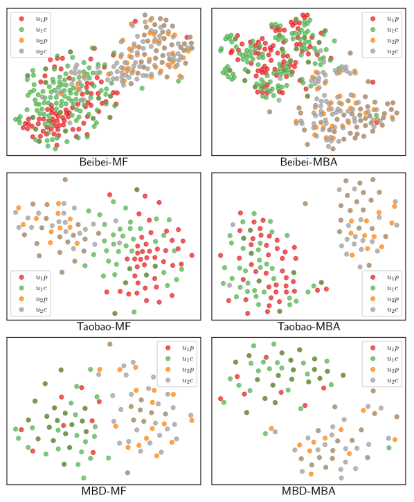
Figure 2. Distributions of items interacted with by two users in the Beibei, Taobao and MBD datasets. Item representations in the graphs on the left are obtained by a matrix factorization model trained on the purchase behavior data, while item representations in the right column graphs are obtained by MBA. $u_{i}c$ ($u_{i}p$) represents the distribution of items clicked (purchased) by user $u_{i}$.

The results show that both parts (KL-divergence and pre-trained models) are essential to MBA because removing either will lead to a performance decrease. Without KL-divergence, we see the performance drops substantially in terms of all metrics. Hence, the KL-divergence helps align the user preferences learned from different behaviors, thus improving the recommendation performance. Without pre-trained models, the results drop dramatically, especially in the Taobao dataset, which indicates that it is hard to co-train $P(\mathbf{R}_{f})$ and $P(\mathbf{R}_{g})$ with MBA. Using a pre-trained model can reduce MBA’s complexity and provide prior knowledge so that it can more effectively extract the user’s real preferences from the different types of behavior distributions.

5.4.2. Hyperparameter study

Next, we conduct experiments to examine the effect of different parameter settings on MBA. Figure 3 shows the effect of $\alpha$, which is used to control the weight of the KL-divergence in conveying information. On the Beibei dataset, the performance of MBA is affected when the $\alpha$ is greater than or equal to 100. Thus, when dominated by KL-divergence, MBA’s performance will be close to that of the pre-trained models. On the Taobao and MBD datasets, when $\alpha$ is greater than or equal to 100, MBA will gradually converge, with a relatively balanced state between the KL-divergence and the expectation term. Under this setting, MBA achieves the best performance.

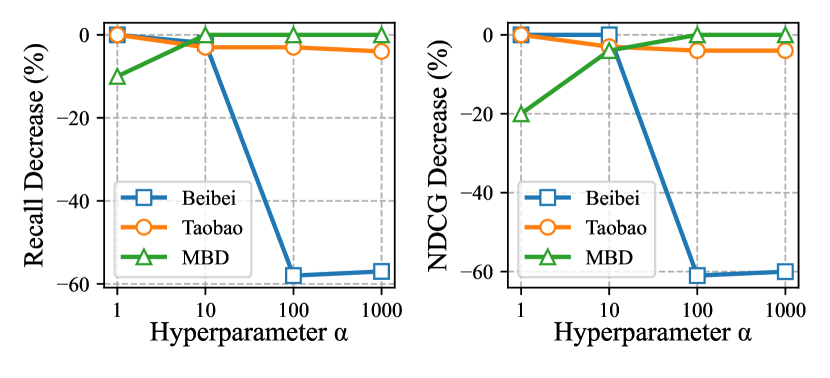
Figure 3. Impact of the hyperparameter $\alpha$.

6. Conclusion

In this work, we have focused on the task of multi-behavior recommendation. We conjectured that multiple types of behavior from the same user reflect similar underlying user preferences. To tackle the challenges of the gap between data distributions of different types of behavior and the challenge of behavioral data being noisy and biased, we proposed a learning framework, namely multi-behavior alignment (MBA), which can infer universal user preferences from multiple types of observed behavioral data, while performing data denoising to achieve beneficial knowledge transfer. Extensive experiments conducted on three real-world datasets showed the effectiveness of the proposed method.

Our method proves the value of mining the universal user preferences from multi-behavior data for the implicit feedback-based recommendation. However, a limitation of MBA is that it can only align between two types of behavioral data. As to our future work, we aim to perform alignment on more types of user behavior. In addition, we plan to develop ways of conducting more effective and efficient model training.

- (1)
- Chen et al. (2021a) Chong Chen, Weizhi Ma, Min Zhang, Zhaowei Wang, Xiuqiang He, Chenyang Wang, Yiqun Liu, and Shaoping Ma. 2021a. Graph Heterogeneous Multi-relational Recommendation. In Proceedings of AAAI.
- Chen et al. (2020b) Chong Chen, Min Zhang, Yongfeng Zhang, Weizhi Ma, Yiqun Liu, and Shaoping Ma. 2020b. Efficient Heterogeneous Collaborative Filtering without Negative Sampling for Recommendation. In Proceedings of AAAI.
- Chen et al. (2022) Huiyuan Chen, Yusan Lin, Menghai Pan, Lan Wang, Chin-Chia Michael Yeh, Xiaoting Li, Yan Zheng, Fei Wang, and Hao Yang. 2022. Denoising Self-attentive Sequential Recommendation. In Proceedings of RecSys.
- Chen et al. (2021c) Huiyuan Chen, Lan Wang, Yusan Lin, Chin-Chia Michael Yeh, Fei Wang, and Hao Yang. 2021c. Structured Graph Convolutional Networks with Stochastic Masks for Recommender Systems. In Proceedings of SIGIR.
- Chen et al. (2020a) Jiawei Chen, Hande Dong, Xiang Wang, Fuli Feng, Meng Wang, and Xiangnan He. 2020a. Bias and Debias in Recommender System: A Survey and Future Directions. CoRR (2020).
- Chen et al. (2021b) Jiawei Chen, Xiang Wang, Fuli Feng, and Xiangnan He. 2021b. Bias Issues and Solutions in Recommender System. In Proceedings of RecSys.
- Cheng et al. (2023) Zhiyong Cheng, Sai Han, Fan Liu, Lei Zhu, Zan Gao, and Yuxin Peng. 2023. Multi-Behavior Recommendation with Cascading Graph Convolution Networks. In Proceedings of WWW.
- Ding et al. (2018) Jingtao Ding, Fuli Feng, Xiangnan He, Guanghui Yu, Yong Li, and Depeng Jin. 2018. An Improved Sampler for Bayesian Personalized Ranking by Leveraging View Data. In Proceedings of WWW.
- Ding et al. (2019a) Jingtao Ding, Yuhan Quan, Xiangnan He, Yong Li, and Depeng Jin. 2019a. Reinforced Negative Sampling for Recommendation with Exposure Data.. In Proceedings of IJCAI.
- Ding et al. (2019b) Jingtao Ding, Guanghui Yu, Xiangnan He, Fuli Feng, Yong Li, and Depeng Jin. 2019b. Sampler Design for Bayesian Personalized Ranking by Leveraging View Data. TKDE (2019).
- Gantner et al. (2012) Zeno Gantner, Lucas Drumond, Christoph Freudenthaler, and Lars Schmidt-Thieme. 2012. Personalized Ranking for Non-uniformly Sampled Items. In Proceedings of KDD.
- Gao et al. (2019) Chen Gao, Xiangnan He, Dahua Gan, Xiangning Chen, Fuli Feng, Yong Li, Tat-Seng Chua, and Depeng Jin. 2019. Neural Multi-task Recommendation from Multi-behavior Data. In Proceedings of ICDE.
- Gao et al. (2022) Yunjun Gao, Yuntao Du, Yujia Hu, Lu Chen, Xinjun Zhu, Ziquan Fang, and Baihua Zheng. 2022. Self-guided Learning to Denoise for Robust Recommendation. In Proceedings of SIGIR.
- Gu et al. (2020) Yulong Gu, Zhuoye Ding, Shuaiqiang Wang, and Dawei Yin. 2020. Hierarchical User Profiling for E-commerce Recommender Systems. In Proceedings of WSDM.
- He et al. (2020) Xiangnan He, Kuan Deng, Xiang Wang, Yan Li, Yongdong Zhang, and Meng Wang. 2020. LightGCN: Simplifying and Powering Graph Convolution Network for Recommendation. In Proceedings of SIGIR.
- Huang et al. (2019) Chao Huang, Xian Wu, Xuchao Zhang, Chuxu Zhang, Jiashu Zhao, Dawei Yin, and Nitesh V Chawla. 2019. Online Purchase Prediction via Multi-scale Modeling of Behavior Dynamics. In Proceedings of KDD.
- Jagerman et al. (2019) Rolf Jagerman, Harrie Oosterhuis, and Maarten de Rijke. 2019. To Model or To Intervene: A Comparison of Counterfactual and Online Learning to Rank from User Interactions. In Proceedings of SIGIR.
- Jin et al. (2020) Bowen Jin, Chen Gao, Xiangnan He, Depeng Jin, and Yong Li. 2020. Multi-behavior Recommendation with Graph Convolutional Networks. In Proceedings of SIGIR.
- Kim et al. (2014) Youngho Kim, Ahmed Hassan, Ryen W White, and Imed Zitouni. 2014. Modeling Dwell Time to Predict Click-level Satisfaction. In Proceedings of WSDM.
- Kingma and Ba (2015) Diederik P Kingma and Jimmy Ba. 2015. Adam: A Method for Stochastic Optimization. In Proceedings of ICLR.
- Koren et al. (2009) Yehuda Koren, Robert Bell, and Chris Volinsky. 2009. Matrix Factorization Techniques for Recommender Systems. Computer (2009).
- Lu et al. (2019) Hongyu Lu, Min Zhang, Weizhi Ma, Ce Wang, Feng Xia, Yiqun Liu, Leyu Lin, and Shaoping Ma. 2019. Effects of User Negative Experience in Mobile News Streaming. In Proceedings of SIGIR.
- Ma et al. (2022b) Muyang Ma, Pengjie Ren, Zhumin Chen, Zhaochun Ren, Lifan Zhao, Peiyu Liu, Jun Ma, and Maarten de Rijke. 2022b. Mixed Information Flow for Cross-domain Sequential Recommendations. TKDD (2022).
- Ma et al. (2022a) Wanqi Ma, Xiancong Chen, Weike Pan, and Zhong Ming. 2022a. VAE++ Variational AutoEncoder for Heterogeneous One-Class Collaborative Filtering. In Proceedings of WSDM.
- Meng et al. (2020) Wenjing Meng, Deqing Yang, and Yanghua Xiao. 2020. Incorporating User Micro-behaviors and Item Knowledge into Multi-task Learning for Session-based Recommendation. In Proceedings of SIGIR.
- Pan et al. (2019) Feiyang Pan, Shuokai Li, Xiang Ao, Pingzhong Tang, and Qing He. 2019. Warm up Cold-start Advertisements: Improving CTR Predictions via Learning to Learn ID Embeddings. In Proceedings of SIGIR.
- Pan et al. (2010) Weike Pan, Evan Xiang, Nathan Liu, and Qiang Yang. 2010. Transfer Learning in Collaborative Filtering for Sparsity Reduction. In Proceedings of AAAI.
- Rendle et al. (2009) Steffen Rendle, Christoph Freudenthaler, Zeno Gantner, and Lars Schmidt-Thieme. 2009. BPR: Bayesian Personalized Ranking From Implicit Feedback. In Proceedings of UAI.
- Rendle et al. (2020) Steffen Rendle, Walid Krichene, Li Zhang, and John Anderson. 2020. Neural Collaborative Filtering vs. Matrix Factorization Revisited. In Proceedings of RecSys.
- Shen and Sanghavi (2019) Yanyao Shen and Sujay Sanghavi. 2019. Learning With Bad Training Data via Iterative Trimmed Loss Minimization. In Proceedings of ICML.
- Tsagkias et al. (2020) Manos Tsagkias, Tracy Holloway King, Surya Kallumadi, Vanessa Murdock, and Maarten de Rijke. 2020. Challenges and Research Opportunities in Ecommerce Search and Recommendations. SIGIR Forum (2020).
- Wang et al. (2021a) Wenjie Wang, Fuli Feng, Xiangnan He, Liqiang Nie, and Tat-Seng Chua. 2021a. Denoising Implicit Feedback for Recommendation. In Proceedings of WSDM.
- Wang et al. (2020) Wen Wang, Wei Zhang, Shukai Liu, Qi Liu, Bo Zhang, Leyu Lin, and Hongyuan Zha. 2020. Beyond clicks: Modeling Multi-relational Item Graph for Session-based Target Behavior Prediction. In Proceedings of WWW.
- Wang et al. (2019) Xiang Wang, Xiangnan He, Meng Wang, Fuli Feng, and Tat-Seng Chua. 2019. Neural Graph Collaborative Filtering. In Proceedings of SIGIR.
- Wang et al. (2022) Yu Wang, Xin Xin, Zaiqiao Meng, Joemon M Jose, Fuli Feng, and Xiangnan He. 2022. Learning Robust Recommenders through Cross-Model Agreement. In Proceedings of WWW.
- Wang et al. (2021b) Zitai Wang, Qianqian Xu, Zhiyong Yang, Xiaochun Cao, and Qingming Huang. 2021b. Implicit Feedbacks are Not Always Favorable: Iterative Relabeled One-Class Collaborative Filtering against Noisy Interactions. In Proceedings of ACMMM.
- Wei et al. (2022) Wei Wei, Chao Huang, Lianghao Xia, Yong Xu, Jiashu Zhao, and Dawei Yin. 2022. Contrastive Meta Learning with Behavior Multiplicity for Recommendation. In Proceedings of WSDM.
- Wu et al. (2021) Jiancan Wu, Xiang Wang, Fuli Feng, Xiangnan He, Liang Chen, Jianxun Lian, and Xing Xie. 2021. Self-supervised Graph Learning for Recommendation. In Proceedings of SIGIR.
- Xia et al. (2021) Lianghao Xia, Yong Xu, Chao Huang, Peng Dai, and Liefeng Bo. 2021. Graph Meta Network for Multi-behavior Recommendation. In Proceedings of SIGIR.
- Xie et al. (2021) Ruobing Xie, Cheng Ling, Yalong Wang, Rui Wang, Feng Xia, and Leyu Lin. 2021. Deep Feedback Network for Recommendation. In Proceedings of IJCAI.
- Xie et al. (2020) Ruobing Xie, Zhijie Qiu, Jun Rao, Yi Liu, Bo Zhang, and Leyu Lin. 2020. Internal and Contextual Attention Network for Cold-start Multi-channel Matching in Recommendation.. In Proceedings of IJCAI.
- Xuan et al. (2023) Hongrui Xuan, Yi Liu, Bohan Li, and Hongzhi Yin. 2023. Knowledge Enhancement for Multi-Behavior Contrastive Recommendation. In Proceedings of WSDM.
- Yu and Qin (2020) Wenhui Yu and Zheng Qin. 2020. Sampler Design for Implicit Feedback Data by Noisy-label Robust Learning. In Proceedings of SIGIR.
- Yuan et al. (2022) Jiahao Yuan, Wendi Ji, Dell Zhang, Jinwei Pan, and Xiaoling Wang. 2022. Micro-Behavior Encoding for Session-based Recommendation. In Proceedings of ICDE.
- Zhao et al. (2016) Qian Zhao, Shuo Chang, F Maxwell Harper, and Joseph A Konstan. 2016. Gaze Prediction for Recommender Systems. In Proceedings of RecSys.
- Zhou et al. (2018) Meizi Zhou, Zhuoye Ding, Jiliang Tang, and Dawei Yin. 2018. Micro Behaviors: A New Perspective in E-commerce Recommender Systems. In Proceedings of WSDM.
- Zhu et al. (2018) Han Zhu, Xiang Li, Pengye Zhang, Guozheng Li, Jie He, Han Li, and Kun Gai. 2018. Learning Tree-based Deep Model for Recommender Systems. In Proceedings of KDD.
- Zhu et al. (2021) Yongchun Zhu, Kaikai Ge, Fuzhen Zhuang, Ruobing Xie, Dongbo Xi, Xu Zhang, Leyu Lin, and Qing He. 2021. Transfer-meta Framework for Cross-domain Recommendation to Cold-start Users. In Proceedings of SIGIR.