Electricity Load and Peak Forecasting: Feature Engineering, Probabilistic LightGBM and Temporal Hierarchies

Abstract

We describe our experience in developing a predictive model that placed high position in the BigDeal Challenge 2022, an energy competition of load and peak forecasting. We present a novel procedure for feature engineering and feature selection, based on cluster permutation of temperatures and calendar variables. We adopted gradient boosting of trees and we enhance its capabilities with trend modelling and distributional forecasts. We also include an approach to forecast combination known as temporal hierarchies, which further improves the accuracy.

Keywords Load Forecasting Feature engineering Gradient Boosting Hierarchical Forecasting Temporal reconciliation BigDEAL Challenge 2022

Introduction

Load forecasting is the problem of predicting the future profile of power demand, while peak forecasting is the problem of predicting the maximum (e.g. daily) value of demand and the time of its occurrence. Peak forecasting is important because often decision making is based on the forecast of the peak rather then on the forecast of the entire load profile.

In this work we present an approach that successfully competed in the BIGDeal Challenge 2022 [21], which was about energy load and peak forecasting. The competition was held in October-December 2022; 121 contestants took part, divided in 78 teams. The forecasts were assessed using different indicators and the competition was split into a qualifying match and a final match. We achieved the $3^{rd}$ position in the qualifying match, gaining access to the final match, where we ended $6^{th}$ [22].

For the qualifying match we used Gradient Boosting (GB) of trees, coupled with an original method of feature engineering and feature selection. For the final match, we developed a more sophisticated approach. In particular, we adopted a recent probabilistic version of LightGBM [38]; we used the DART algorithm [45] for regularization, and we also used temporal hierarchies [3] in order to improve the forecasts by combining predictions at different temporal scales. Even though the competition only scored the point forecasts, our approach is probabilistic, and thus quantifies the uncertainty of the forecasts. This is indeed needed to support decision making.

The paper is organized as follows. Next an outlook of long-term load forecasting and our motivations are given. We introduce Gradient Boosting (GB) of trees and probabilistic extensions in Sec. Gradient Boosting and Distributional forecasts. We present our approach for feature engineering for load forecasting in Sec. Feature Engineering, and feature selection in Sec. Feature Selection. Temporal hierarchies are presented in Sec. Temporal hierarchies. In Sec. Experiments we detailed review our pipeline with technical insights, and competition results. We end this work with a critical Conclusion.

Methodology

Long-term Load Forecasting

Load forecasting is the problem of predicting the electricity demand of the next $H$ time steps, denoted by $[y_{T+1},\,\ldots\,,y_{T+H}]$. When the order of magnitude of $H$ is a few hundreds or more, we talk about long-term forecasting. For instance, forecasting a year-ahead at hourly scale implies producing 24 $\times$ 365 = 8760 forecasts. Classical forecasting strategies [4] condition the forecast on the last observations of the time series. However, this is not viable for long-term forecasting, since in this case $y_{T+H}$ is independent from $y_{T}$. Long-term forecasting is better addressed as a regression problem, adopting a rich set of explanatory variables (features) [27, 15, 8, 46] regarding calendar effect (the day of the week, hour of the day, etc), holidays, temperature, etc. This approach allows adopting regression methods such as Gradient Boosting (GB) of trees [16], which is indeed successful in long-term energy forecasting [44].

Gradient Boosting and Distributional forecasts

In fact, GB achieved top positions in the Global Energy Forecasting Competitions (GEFCom) of 2012, 2014, 2017 [24, 25, 26], in the M5 forecasting competition [35, 29] and in competitions on tabular data [7, 42]. The most popular implementations are XGBoost [9], LightGBM [30] and CatBoost [12]. They have comparable accuracy, but LightGBM is generally faster and scales better on large data sets.

GB can be trained with different loss function besides the traditional least squares. For instance, GB trained to perform quantile regression won the GEFCom2014 probabilistic competition [17]. Yet, even quantile regression only returns a point forecasts without a predictive distribution. It is possible to train different GB models, one for each desired quantile; but if the predicted quantiles cross, the predictive distribution is invalid [39, 41]. The recent versions of probabilistic GB of trees constitute a sounder approach [13, 37, 38] to probabilistic forecasting. In this paper we adopt the model of März et al. [38], which returns a multivariate output containing the moments of the predictive distribution.

A successful implementation of GB requires anyway paying attention to some possible issues. For instance, GB is is generally unable to model a long-term trend. If the time series is trendy, it is recommended to detrend it, fit the GB model, and then add the predicted trend to the GB forecast [50, 33, 47]. Another pre-processing step which is sometimes helpful is a logarithmic transformation which stabilizes the variance of the target time series [43]. Moreover, GB is subject to overfitting. The DART algorithm [45] solves the problem introducing Dropout regularization, analogously to Neural Networks.

Feature Engineering

The exogenous variables that are frequently used in load forecasting are related to calendar and temperatures.

Calendar-based features

Calendar variables allow to capture the seasonal patterns. They are commonly modeled by categorical variables, using one category for each value of the feature. For example, the day of the week is represented by a categorical variable with seven levels. Holidays are represented by a binary variable with two levels: 1 for holiday and 0 for non-holiday.

Lagged and rolling temperatures

Temperature impacts on energy consumption, by driving the use of heating, ventilation, and air conditioning (HVAC) systems. However, there is generally a delay between the change in temperature and the change in energy consumption. We thus consider the lagged hourly temperatures:

$$T(t-h),\qquad h=1,2,\,\dots\,,L$$ (1)

where $L$ is the maximum lag, and moving/rolling temperature’s statistics:

$$T_{f}^{w}(t)=f(T(t-1),\,\dots\,,T(t-w))$$ (2)

where $f(\cdot)$ is some statistical function and $w$ indicates the width of the window of past values of hourly temperatures considered. For example, the moving average of the last 24 hours of temperature values is $T_{avg}^{24}(t)=\frac{1}{24}\sum_{h=1}^{24}{T(t-h)}$.

Aggregated indicators of temperature

Aggregated features can capture longer-term effect of temperature on energy load, smoothing out noise in the data. They can be expressed as $\tilde{T}_{f}^{g}(t)$ where $g$ is the aggregation period and $f(\cdot)$ is the aggregation function. This features includes, for example, the daily maximum and minimum values of the temperature or the monthly standard deviation of the temperature.

In this paper we propose additional aggregation functions (Tab. 1) borrowed from signal processing [14, 49], which to the best of our knowledge have been not yet used in energy forecasting. The signal processing features should be computed on the time series of temperature, rescaled to have zero mean in the selected aggregation period. They provide insights about the variability and shape of the temperature profile within the aggregation period. For example, the crest factor measures the peak-to-average ratio of a signal. A high daily crest factor corresponds to large variations of temperature during the day, which generally increase energy demand. On the other hand, a low daily crest factor corresponds to stable temperatures during the day, which generally decreases energy demand.

Table 1: Signal Processing features for load forecasting.

RMS	$x_{RMS}=\sqrt{\frac{1}{N}\sum_{i=1}^{N}x_{i}^{2}}$
Peak value	$x_{p}=\max(\left|x_{i}\right|)$
Crest factor	$x_{crest}=\frac{x_{p}}{x_{RMS}}$
Impulse factor	$x_{if}=\frac{x_{p}}{\frac{1}{N}\sum_{i=1}^{N}{\left|x_{i}\right|}}$
Margin factor	$x_{mf}=\frac{x_{p}}{\left(\sum_{i=1}^{N}\left|x_{i}\right|^{1/2}\right)^{2}}$
Shape factor	$x_{sf}=\frac{x_{RMS}}{\frac{1}{N}\sum_{i=1}^{N}{\left|x_{i}\right|}}$
Peak to peak value	$x_{pp}=\max(x_{i})-\min(x_{i})$

Feature Selection

Feature engineering generally generates a large set of features, many of which are eventually redundant. Hence, feature selection is needed to: shorten the training times [32], reduce overfitting [6], improve the model interpretability [28].

We perform feature selection based on hierarchical clustering and pairwise correlation of the features. The core block of our approach is Permutation Feature Importance (PFI), which measures the drop in performance when a feature is randomly shuffled. It has foundations in [5, 40]. The size of the drop of performance shows how much the model relies on that feature for predictions. PFI is appealing since:

• it can be applied to any model;

• it is easy to implement (Algorithm 1);

• it can measure feature importance on the metric of the competition;

• it can be computed out-of-sample.

Algorithm 1 Permutation Feature Importance

A trained model and recorded score $s$ on an evaluation dataset.

for feature $x_{j},j=1,\dots,d$ do

     for each repetition $k,k=1,\dots,K$ do

         Randomly shuffle column $j$ of the original evaluation set.

         Compute new score $s_{k,j}$ of the model on the perturbed set.

     end for

     Compute importance of feature $x_{j}$ as:

$$I_{j}=s-\frac{1}{K}\sum_{k=1}^{K}{s_{k,j}}$$

end for

However, shuffling a single features can produce unrealistic samples if features are dependent. Furthermore, correlated features share importance, therefore their relevance may be underestimated (substitution effect) [20, 40].

Clustered Permutation Feature Importance

To overcome such issues we propose a novel approach, which we call Clustered Permutation Feature Importance (CPFI). The method works as follows. At first, groups of highly correlated features are identified by applying hierarchical clustering on the correlation matrix of the features. To form the correlation matrix, a measure of dependence between each feature pair is computed using a correlation index, Pearson’s or Spearman’s for instance. Then, we jointly shuffle all the variables of the same cluster and we compute the subsequent performance drop. The more orthogonal is the information contained in different clusters, the more reliable is the estimate of importance.

Finally, we drop non-informative feature clusters from the model. On the contrary, we keep in the model the features of the relevant clusters. Also, only one or few features can be selected from each group based on some measure of explanatory with respect to the target, or some expert advice. We propose a criterion to discriminate informative from non-informative cluster of features in Sec. Experiments. Similar approaches have already been proposed in finance [11] and biochemistry [36].

Temporal hierarchies

As a further tool to improve the forecasting accuracy, we consider temporal hierarchies [3]. For instance, assume that we want to generate forecasts at the hourly scale (referred to as the bottom level). A temporal hierarchy creates forecasts also at coarser temporal scales (e.g., 2-hourly and 4-hourly) and then combines information from the forecasts generated at the different temporal scales. This process generally improves the forecasting accuracy at all levels [3, 31]. A temporal hierarchy works as follows. First, forecasts are independently created at the different temporal scales (base forecasts). For instance, Fig. 1 shows a temporal hierarchy aimed at forecasting 4-hours ahead. It contains 4 forecasts computed at hourly frequency ($\hat{h}_{1},...,\hat{h}_{4}$, bottom level); two forecasts computed at 2-hour frequency ($\hat{h}_{12},...,\hat{h}_{34}$, intermediate level); one forecast computed at 4-hour frequency ($\hat{h}_{1234}$, top level).

Generally the base forecasts do not sum up correctly and they are referred to as incoherent. For instance: $\hat{h}_{12}\neq\hat{h}_{1}+\hat{h}_{2}$, $\hat{h}_{34}\neq\hat{h}_{3}+\hat{h}_{4}$, etc. Reconciliation [48] is the process of adjusting the base forecast so that they become coherent, i.e., they sum up correctly. The reconciled forecasts are denoted with a tilde and thus in the example of Fig. 1 after reconciliation we have: $\tilde{h}_{12}=\tilde{h}_{1}+\tilde{h}_{2}$, $\tilde{h}_{34}=\tilde{h}_{3}+\tilde{h}_{4}$, $\tilde{h}_{1234}=\tilde{h}_{12}+\tilde{h}_{34}$.

Figure 1: Temporal hierarchy for forecasting 4-hours ahead, using hourly forecasts (bottom level), 2-hourly forecasts and 4-hourly forecasts.

Temporal hierarchies require the mean and the variance of the base forecasts. The original algorithm [3] provides only the reconciled point forecast, while the approach of [10] yields also a reconciled predictive distribution.

Experiments

The BigDEAL Challenge 2022 was divided in a qualifying match and a final match.

The qualifying match provided hourly load and hourly temperature statistics (mean, median, min, max) of four weather stations for the period 2002-2006; see Fig. 2 for an example. It required to forecast year 2007 given the actual temperatures. This is referred to as a ex-post setting [27].

The final match provided three years (2015-2017) of hourly load of three U.S. local distribution companies (LDC), and hourly temperatures from six weather station. The forecasted (ex-ante setting [27]) 1-day ahead temperatures for 2018 were released on a rolling basis, two months at a time. The forecasts for these periods were to be delivered, in a total of six consecutive rounds.

Both matches required forecasts at hourly scale for the 24h, the values of the peak for each day, and its time of occurrence (i.e. a discrete number between 1 and 24).

The organizers ran two baseline methods. The first is Tao’s Vanilla Benchmark [24], namely a multiple linear regression whose features are trend, calendar effects, and only a single feature related to the temperature. The second is the Recency Benchmark [46], which extends the previous model by including many features related to temperatures, among which lagged values and moving averages.

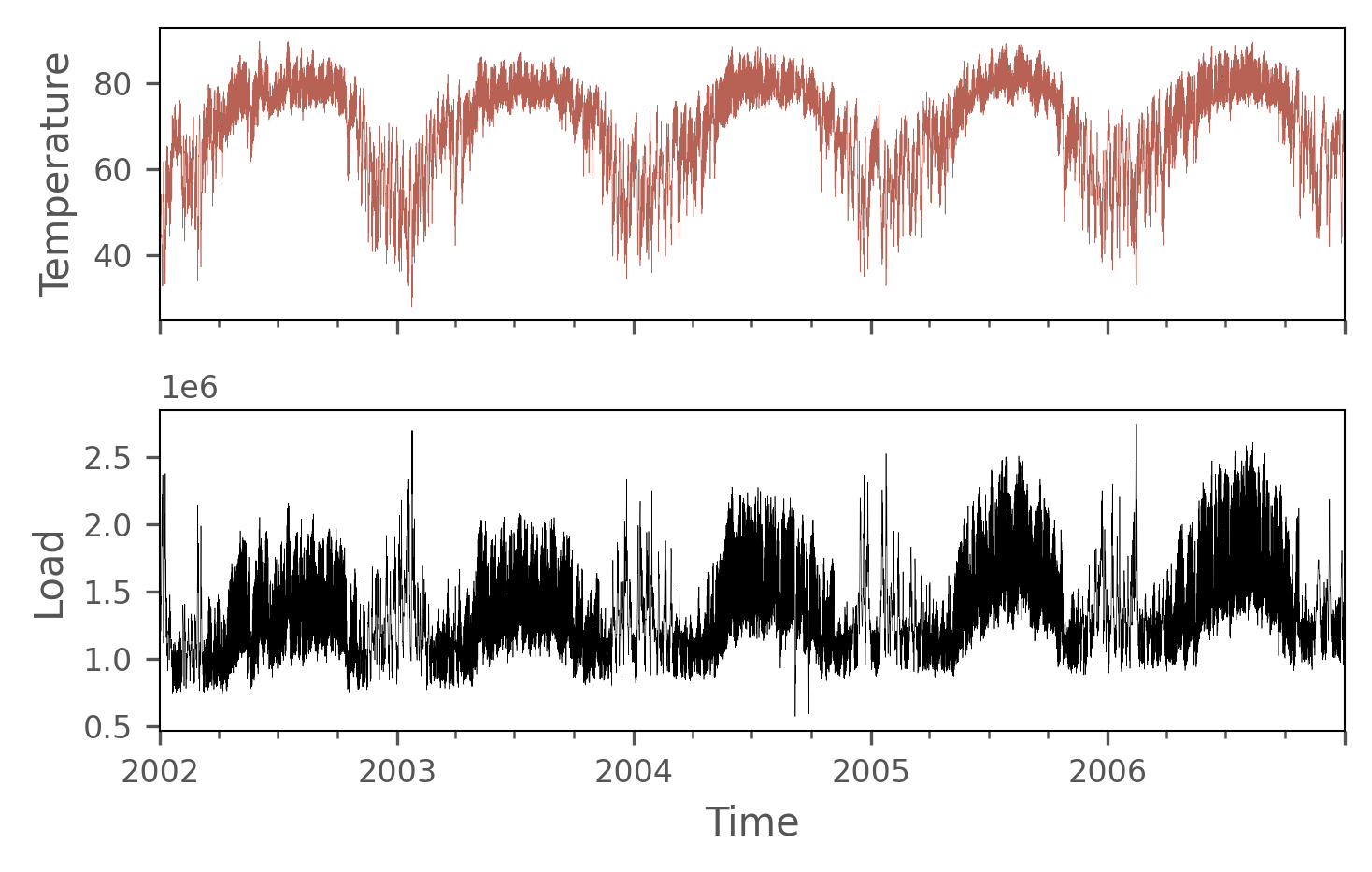
Figure 2: Load (MW) and temperature $\text{T}_{avg}$ (°F) of the qualifying match of the BigDEAL challenge. For readability, we show data aggregated over 12 hours.

Performance measures

The organizers evaluated the forecasts of each match with three different tracks.

In the qualifying match the hourly forecasts ($24\times 365=8760$) were scored using the Mean Absolute Percentage Error (MAPE):

$$\text{MAPE}=\frac{1}{H}\sum_{t=T+1}^{T+H}{\frac{|y_{t}-\hat{y}_{t}|}{|y_{t}|}\times 100},$$ (3)

where $y_{t}$ and $\hat{y}_{t}$ denote the actual and the forecasted value for time $t$. The second metrics was the Magnitude (M); it is the MAPE between the actual and forecasted daily peak values (i.e., it refers to 365 forecasts with one year horizon). However, we recall that MAPE has been criticized in the forecasting literature: it penalizes over-estimation errors more than under-estimation ones [2] and moreover it is numerically unstable when dealing with values close to 0.

To score the prediction of peak hours the organizers used a third metric, called Timing (T), which computes the Mean Absolute Error. For example, if actual peak is at 6pm, and forecasted peak time is at 8pm, the error for that day is $|6-8|=2$.

The final match scored the forecasts using Magnitude (M) and Timing (T), plus an additional metric called Shape (S). However, the definition of Timing was modified introducing a non-uniform cost for the error. Let us denote by $\mathcal{T}_{d}$ and $\hat{\mathcal{T}}_{d}$ the actual and the forecasted peak hour for a day $d$. Timing was then defined as:

$$\text{T}=\frac{1}{\left|days\right|}\sum_{d\,\text{in}\,days}w(\mathcal{T}_{d},\hat{\mathcal{T}}_{d}),\text{with}$$ (4)

$$w(\mathcal{T}_{d},\hat{\mathcal{T}}_{d})=\begin{cases}|\mathcal{T}_{d}-\hat{\mathcal{T}}_{d}|,&\text{if }|\mathcal{T}_{d}-\hat{\mathcal{T}}_{d}|=1,\\ 2|\mathcal{T}_{d}-\hat{\mathcal{T}}_{d}|,&\text{if }2\leq|\mathcal{T}_{d}-\hat{\mathcal{T}}_{d}|\leq 4,\\ 10,&\text{if }|\mathcal{T}_{d}-\hat{\mathcal{T}}_{d}|\geq 5\end{cases}$$

Shape (S) scored the shape of the forecast around the peak. To compute it, the 24h load forecasts of a day is normalized by the peak forecast of that day, and the same is done for the actual load. Then the sum of absolute errors during the 5-hour peak period (actual peak hour $\pm$ 2 hours) of every day is calculated. We denote by $\bar{y}_{d}$ and $\bar{\hat{y}}_{d}$ the normalized actual and forecasted load for a day $d$; $\bar{y}_{d}=\frac{y_{d}}{\max{y_{d}}}$, $\bar{\hat{y}}_{d}=\frac{\hat{y}_{d}}{\max{\hat{y}_{d}}}$. Shape is defined as:

$$\text{S}=\frac{1}{\left|days\right|}\sum_{d\,\text{in}\,days}\sum_{t\,\text{in}\,\{\mathcal{T}_{d},\mathcal{T}_{d}\pm 1,\mathcal{T}_{d}\pm 2\}}|\bar{y}_{d}(t)-\bar{\hat{y}}_{d}(t)|$$ (5)

Scoring the Predictive Distribution

While the competition only assessed the point forecasts, we also scored the distributional forecasts obtained from our probabilistic models. In particular, we compared the probabilistic forecast of our GB model (based on [38]) with those obtained after the application of the temporal hierarchy.

We scored the predictive distributions of the model using the Continuous Ranked Probability Score (CRPS) [19]. Let us denote by $\mathbf{\hat{F}}$ the predictive cumulative distribution function and by $y$ the actual value:

$$\text{CRPS}(\mathbf{\hat{F}},y)=\int_{-\infty}^{\infty}(\mathbf{\hat{F}}(x)-\mathbbm{1}(x\geq y))^{2}\,dx$$ (6)

With Gaussian $\mathbf{\hat{F}}$, the integral can be computed in closed form [19].

We then scored the prediction intervals using the Interval Score (IS) [18]. Let us denote by $1-\alpha$ the nominal coverage of the interval (assumed 0.9 in this paper), by $\mathbf{l}$ and $\mathbf{u}$ its lower and upper bound. We thus computed with the models, for each hour, a $90\%$ prediction interval and the score:

$$\text{IS}(\mathbf{l},\mathbf{u},y)=(\mathbf{u}-\mathbf{l})+\frac{2}{\alpha}(\mathbf{l}-y)\mathbbm{1}(y<\mathbf{l})+\frac{2}{\alpha}(y-\mathbf{u})\mathbbm{1}(y>\mathbf{u})\,.$$ (7)

We also report the proportion of cases in which the interval ($\mathbf{l},\mathbf{u}$) contains $y$.

Skill score

Let $m_{origin}$ and $m_{new}$ two comparable metrics. We denote the positive or negative percentage improvement by the Skill score defined as:

$$\text{Skill}_{\%}(m_{origin},m_{new})=\frac{m_{origin}-m_{new}}{(m_{origin}+m_{new})/2}\times 100$$ (8)

Qualifying Match

Below we present the building blocks of our implementation.

Cross-validation strategy

Given the sequential nature of the data, time series cross-validation was used to evaluate the performance of each model, hyper-parameter tuning and feature selection. This method involves partitioning the data into an in-sample data set comprising earlier observations, and an out-of-sample data set containing the most recent observations. The model is trained on the in-sample part and evaluated on the out-of-sample part. To obtain multiple evaluations, the out-of-sample set is iteratively shifted forward by a time window, and the model is retrained on the updated in-sample set. This procedure is repeated for all the out-of-sample sets, ensuring that the model is tested on unseen sequences of observations during evaluation, which results in a more realistic assessment.

The size of the time window is typically chosen equal to the size of the test set on which the final prediction is to be made. Hence, for the qualifying phase, years 2004, 2005 and 2006 were used as out-of-sample folds.

Baseline model

We started by modelling basic calendar features (Year, Month, Week, Day, Weekday, Hour) and temperatures at the current time ($\text{T}_{avg}$, $\text{T}_{med}$, $\text{T}_{min}$, $\text{T}_{max}$). Calendar variables were encoded with label encoding. We tested more sophisticated encoding (target encoding, cyclical encoding with sine/cosine transformation and cyclical encoding with radial basis functions) but without notable improvement.

We applied a logarithmic transformation to the target variable to stabilize its variance. Moreover, since the target variable has a long-term increasing trend, we performed detrending. During each round of cross-validation, we fitted a Linear Regression (LR) model ($y_{i}=\beta_{0}+\beta_{1}x_{i}$, where $x_{i}$ are progressive time indices with $i=1,\ldots,T$) to the in-sample data. We subtracted the linear trend from the training data before fitting the LightGBM model. At the prediction stage, we added the predicted linear trend to the out-of-sample predictions, followed by an exponential transformation, to obtain the final forecast. The effect of detrending is shown in Fig. 3. With detrending the residuals of the models have mean 0 as expected; otherwise, they are severely biased. By detrending we reduced the MAPE (H) of the baseline model from 6.18 to 4.81.

Loss function

We trained the LightGBM models using the L2 loss function.

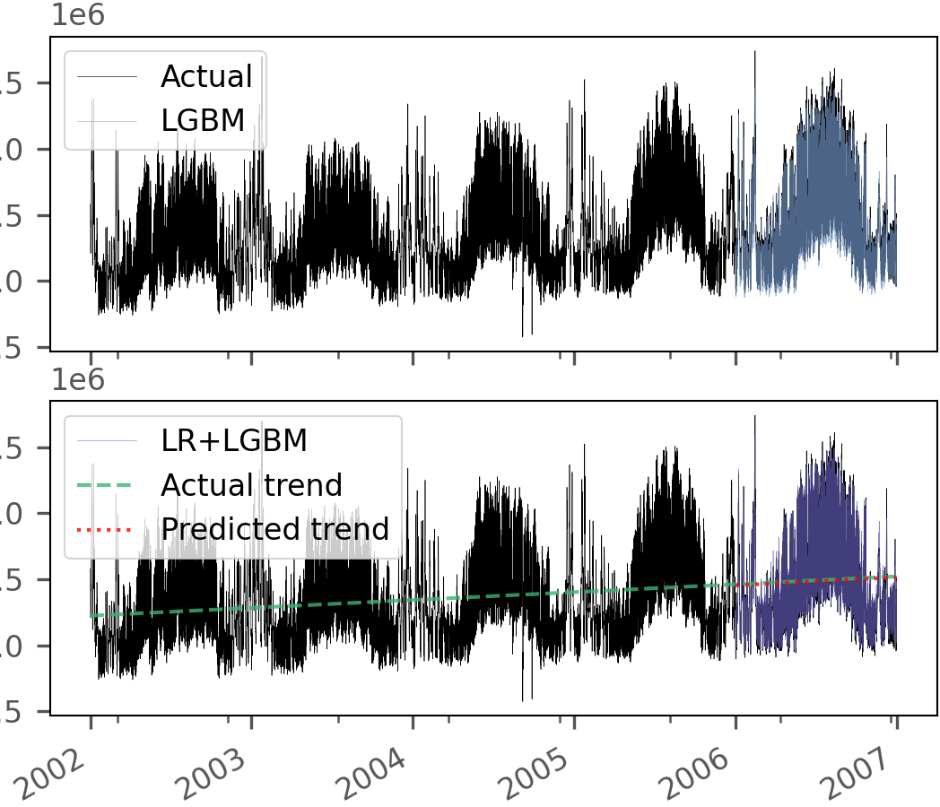
(a) Forecasts

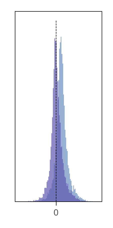
(b) Residuals

Figure 3: The effect of detrending. The LR model ($\beta_{1}=7.05$) corrects the underestimation. The plot of the residuals (on the right) shows how the distribution of the residuals is correctly centered in 0 after detrending.

Outliers

To prevent the models to be biased by outliers, we assigned zero weight to time steps containing these values. We detected them from the left side of the target distribution, which we believe correspond to periods of severe weather conditions.

Feature engineering

Feature engineering was performed incrementally by adding related feature blocks one step at a time. This enabled a systematic evaluation of the impact of each block on the model’s performance while ensuring that every new set of related features provided additional information. We found the following features to be predictive for this competition:

• Additional calendar features: Holiday, Holiday name, Weekend, Week of month, Season, Day of year, Days since last / until next holiday.

• Lagged hourly temperatures: for each temperature variable ($\text{T}_{avg}$, $\text{T}_{med}$, $\text{T}_{min}$, $\text{T}_{max}$) lagged hourly temperatures were incorporated into the model, ranging from a minimum lag of 1 hour to a maximum lag of 48 hours, for a total of 192 new features.

• Temperature-based rolling statistics: for each temperature variable, and for 4 different values of window widths (3 hours, 1 day, 1 week, 1 month), 5 statistical functions (mean, max, min, median, std) were computed, for a total of 80 new features.

• Aggregated temperature statistics: for each temperature variable, for 2 different aggregation time period (Year-Month-Day, Month-Hour), 11 aggregation functions (mean, max, min, median, and centered RMS, crest factor, peak value, impulse factor, margin factor, shape factor, peak to peak value) coupled with the differences between the actual temperature values and the aggregated values were computed for a total of $88\times 2=176$ new features. For clarity, we indicate as an example the daily maximum with the notation $\tilde{T}_{max}^{Year,Month,Day}(t)$, where Year-Month-Day indicates the aggregation to be read from left levels to right.

Feature selection

To evaluate our feature selection strategy, we carried out multiple experiments. First, we assessed the model performance without any feature selection (experiment a). Then, we applied the feature selection strategy described in Sec. Feature Selection after completing all feature engineering, on the entire set of features added to the baseline model (experiment b). Finally, we performed step-by-step feature selection whenever we added a new block of features to the model, i.e. after adding lagged variables, after adding rolling variables, and so on (experiment c). To enhance reliability, cluster permutations were executed 100 times, and mean values and standard deviations of performance drops were calculated against all out-of-sample folds. We consider a cluster of features informative if the importance values fall within three standard deviations of the mean above 0.

Results are presented in Tab. 2. Specifically, the columns for MAPE, Magnitude, and Timing present the results based on the respective competition metrics, whereas columns a, b, and c correspond to the 3 experimental strategies employed.

It is important to note that, unlike experiment a, where the results were obtained in a single training run, the results for experiment b and c were derived from three different training runs, each one maximizing the metric of interest.

Table 2: Out-of-fold qualification results with feature selection methods.

	MAPE (H)			Magnitude			Timing
	a	b	c	a	b	c	a	b	c
Baseline	4.81	-	-	4.43	-	-	1.42	-	-
Calendar	4.83	-	4.78	4.48	-	4.46	1.39	-	1.39
Lags	3.33	-	3.24	3.29	-	3.20	0.94	-	0.92
Roll lags	3.28	-	3.16	3.22	-	3.20	1.06	-	0.94
Agg stats	3.24	3.16	3.09	3.21	3.10	3.08	0.91	0.95	0.91

For illustration purposes, in Fig. 4, we present the feature selection results obtained after incorporating lagged hourly temperatures into the model. Fig. 4a presents the dendrogram obtained from hierarchical clustering computed on the Spearman correlation matrix shown in Fig. 4b. By selecting a threshold value of 0.1, we identified 36 clusters. The cluster rankings that maximize, respectively, the performance of MAPE, Magnitude, and Timing are visible in Fig. 4c. For all the metrics, cluster 8 proved to be the most significant, followed by clusters 31, 7, 2 and 12. This suggests that most informative lags are at t-$\{1,2,3,4,5,6\}$, t-$\{11,12\}$ and t-$\{25,26\}$. Tab. 3 shows the clusters associated feature set.

Table 3: Clustered Permutation Feature Importance: Top-5 clusters of lagged temperatures that maximize performance indicators.

Cluster ID	Feature Set
8	$\text{T}_{avg,med,min}(t-1)$, $\text{T}_{avg,med,min}(t-2)$
31	$\text{T}_{avg,med,min}(t-11)$, $\text{T}_{avg,med,min}(t-12)$
7	$\text{T}_{avg,med,min}(t-3)$, $\text{T}_{avg}(t-4)$
2	$\text{T}_{avg,med,min}(t-5)$, $\text{T}_{avg,med}(t-6)$
12	$\text{T}_{max}(t-1)$, $\text{T}_{max}(t-2)$, $\text{T}_{max}(t-25)$, $\text{T}_{max}(t-26)$

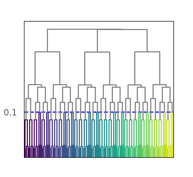
(a) Dendrogram

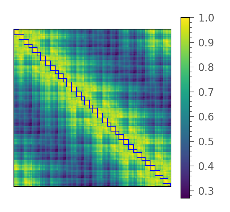
(b) Correlation matrix

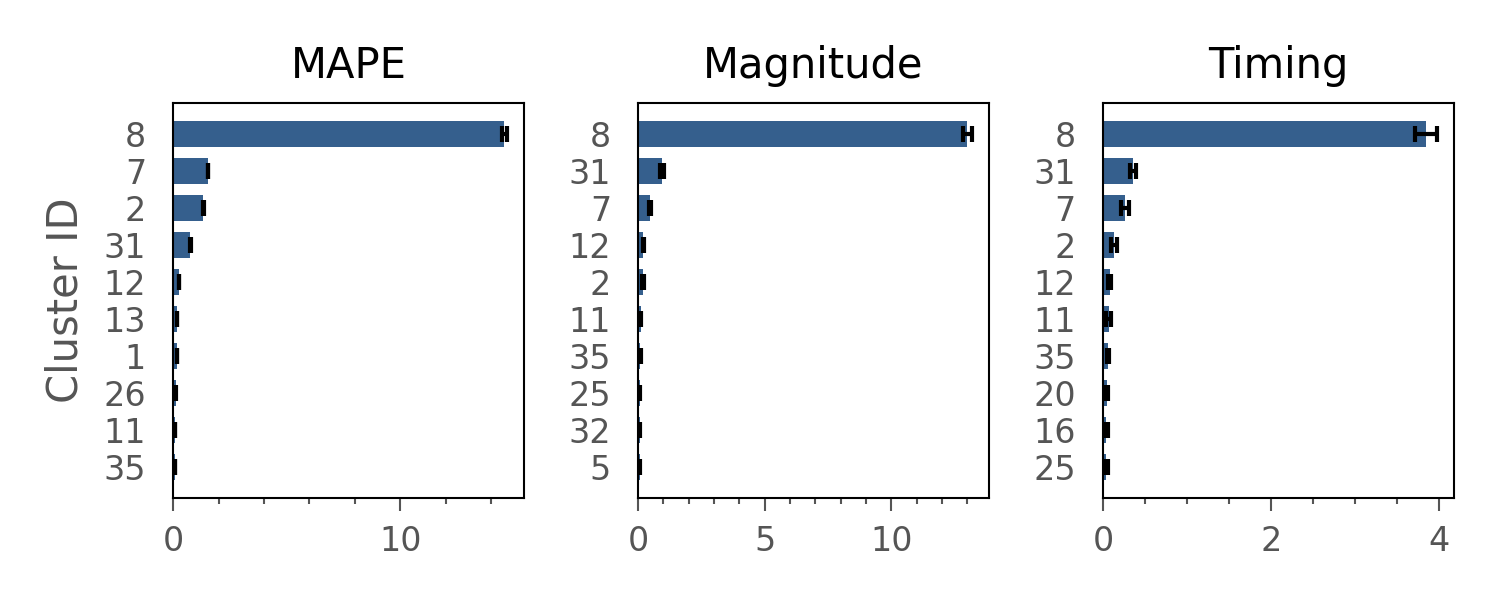
(c) CPFIs

Figure 4: Hierarchical clustering (0.1 threshold) (a) and Spearman’s correlation matrix (b). The blue squares highlight the 36 clusters. In (c) Clustered Permutation Feature Importance (CPFI) values are reported for each track. See Tab. 3 for the Top-5 feature sets.

Hyper-parameter optimization

We used Optuna [1] to tune the learning parameters of LightGBM. It implements time-budget optimization which was useful given the short deadlines of the competition. Another strength of Optuna is that it allows to optimize the parameters with respect to the metric of the competition.

Results

Our team was named “swissknife”; as reported in Tab. 4, we ranked $8^{th}$ on the hourly forecast (H), $3^{rd}$ on the Magnitude (M), $3^{rd}$ on the Timing (T).

Table 4: Leaderboard of Qualifying Match [23].

Team	Rank H.	Team	Rank M.	Team	Rank T.
X-Mines	1	Amperon	1	RandomForecast	1
Amperon	2	Team SGEM KIT	2	Amperon	2
Yike Li	3	swissknife	3	swissknife	3
peaky-finders	4	peaky-finders	4	freshlobster	4
KIT-IAI	5	KIT-IAI	5	peaky-finders	5
Overfitters	6	EnergyHACker	6	Recency Benchmark
BelindaTrotta	7	BelindaTrotta	7	X-Mines	6
swissknife	8	Overfitters	8	BrisDF	7
Recency Benchmark		VinayakSharma	9	BelindaTrotta	8
RandomForecast	9	SheenJavan	10	KIT-IAI	9
Team SGEM KIT	10	…		SheenJavan	10
…		Recency Benchmark	13	…
Tao’s Vanilla Benchmark	27	Tao’s Vanilla Benchmark	25	Tao’s Vanilla Benchmark	30

Final Match

For the final match, we followed the same pipeline tuned in the qualification phase, with the exception of target transformation, which was not required as the target variable was already stationary. Additionally, three LDC loads were to be forecasted (LDC1, LDC2, LDC3) instead of one, and the temperature variables come directly from six weather stations (T1, T2, T3, T4, T5, T6), without aggregate statistics, and moreover without geographical references.

To further enhance performance, we incorporated several techniques, including DART, probabilistic LightGBM and temporal hierarchies.

Feature selection

The most important lagged temperatures were found at time t-$\{1,2,3,4,5\}$, and t-$\{10,11,12\}$ and the most important rolling lag temperatures were found with $w=\{3\,hours,\,1\,day\}$. Fig. 5 shows that within that six weather station, temperatures {T1, T2, T5} better explain LDC1. Hence, our framework nicely handles dataset with multiple weather station.

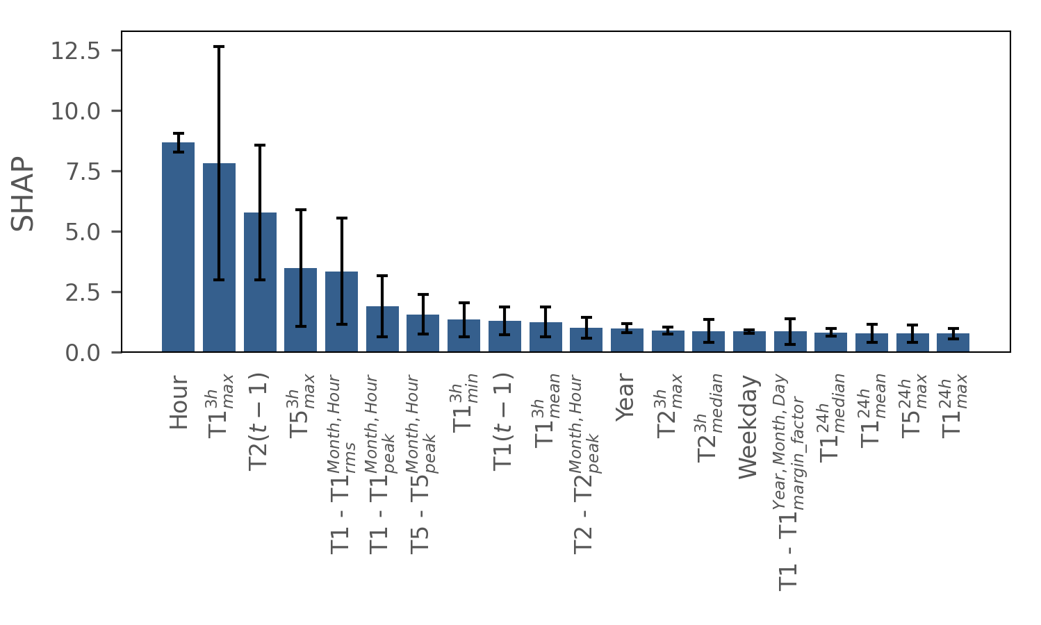
Figure 5: Out-of-fold Top-20 Features Importance obtained after the last incremental step of feature engineering (aggregated features) and feature selection, for LDC1 at Round 1. On the y-axis we reported SHAP (SHapley Additive exPlanations) [34] values of the LightGBM model.

Regularization

The use of DART booster reduce the overfitting that affects LightGBM with standard booster by means of Dropout. However, training becomes slower since it requires more boosting iterations. Additionally, early stopping cannot be used because the algorithm updates previous learned tree during the training. Despite these issues, with DART we reduced the prediction error. Also we find out that the loss decreases steadily and converges asymptotically, even with a large number of boosting iterations. We tested DART on the qualification data only when it was finished. With 30’000 iterations, the MAPE (H) went from 3.24 to 2.83, and Magnitude from 3.21 to 3.09. Therefore, we included DART in the final match model.

Temporal hierarchies

We build a temporal hierarchy by summing the time series of the hourly load and related temperatures at the following scales: 2-hours, 4-hours, 6-hours, 12-hours. We train an independent probabilistic LightGBM-LSS [38] model at each time scale, with DART booster for $30^{\prime}000$ boosting steps. LightGBM-LSS minimizes the Negative Log-Likelihood loss function. Gaussian distributional forecasts were obtained at each temporal scale for the same forecasting horizon $H$. The reconciliation step made base forecasts coherent.

In Tab. 5 (load profile) and Tab. 6 (peak) we compare base and reconciled forecasts, using skill scores ($S_{\%}$); in Fig. 6 we show some forecasts. Temporal hierarchies improve only slightly the point forecasts, but more importantly the predictive distribution, with a skill score of about 5% on CRPS and of about 10% on IS.

We also tested 1-day aggregation without further improvement for the bottom time series. As can be seen from previous feature importance analyses, past values close to the conditioning time are the most important variables for prediction. We come to the explanation that too much aggregation (empirically greater then 1-day) makes these variables vanishing, and temporal hierarchy no longer effective. Instead, small hierarchies also improve peaks, as shown in Tab. 6 and Fig. 6.

Given the availability, the metrics we present for the final match refer to actual competition values of Round 1-5 (Jan-Oct 2018), instead of out-of-fold sets.

Table 5: Reconciliation metrics for the load profiles; base ($\hat{y}$) and reconciled ($\tilde{y}$) forecasts, with skill scores ($S_{\%}$). Temporal hierarchy for forecasting using hourly (bottom level), 2-hourly, 4-hourly, 6-hourly and 12-hourly aggregations.

	MAPE			CRPS			$\text{IS}_{90\%}$			$\text{IC}_{90\%}\,(\%)$
	$\hat{y}$	$\tilde{y}$	$\mathbf{S}_{\%}$	$\hat{y}$	$\tilde{y}$	$\mathbf{S}_{\%}$	$\hat{y}$	$\tilde{y}$	$\mathbf{S}_{\%}$	$\hat{y}$	$\tilde{y}$
LDC1	4.87	4.84	0.75	6.35	6.03	5.16	61.62	55.01	11.34	99.24	98.81
LDC2	5.02	4.99	0.52	10.92	10.44	4.49	101.35	90.39	11.43	99.07	98.49
LDC3	4.51	4.5	0.05	45.99	43.84	4.78	446.49	398.37	11.39	98.85	98.14

Table 6: Reconciliation metrics for the peaks; base ($\hat{y}$) and reconciled ($\tilde{y}$) forecasts, with skill scores ($S_{\%}$). Temporal hierarchy for forecasting using hourly (bottom level), 2-hourly, 4-hourly, 6-hourly and 12-hourly aggregations.

	Magnitude			Timing			Shape			$\text{CRPS}_{\text{peak}}$
	$\hat{y}$	$\tilde{y}$	$\mathbf{S}_{\%}$	$\hat{y}$	$\tilde{y}$	$\mathbf{S}_{\%}$	$\hat{y}$	$\tilde{y}$	$\mathbf{S}_{\%}$	$\hat{y}$	$\tilde{y}$	$\mathbf{S}_{\%}$
LDC1	4.97	4.90	1.34	1.22	1.13	7.93	0.088	0.086	2.16	8.33	7.89	5.46
LDC2	5.51	5.48	0.52	1.26	1.23	1.87	0.102	0.101	1.11	15.73	15.13	3.85
LDC3	4.83	4.79	0.95	1.19	1.09	8.80	0.079	0.078	1.56	60.83	57.97	4.82

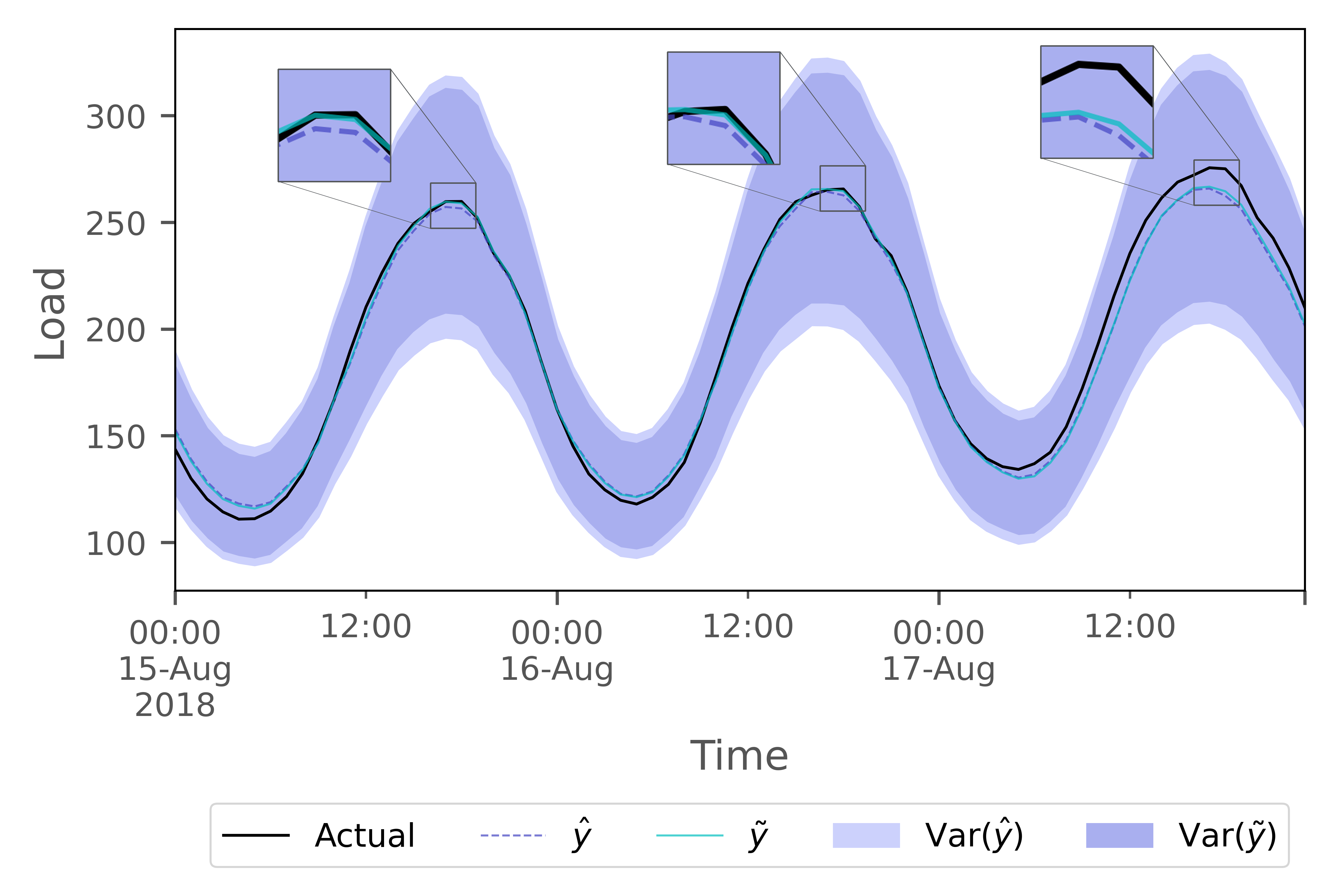
Figure 6: Comparison of probabilistic forecasts, before and after the application of the temporal hierarchy. The temporal hierarchy slightly improves the point forecasts. It also shortens the prediction intervals without compromising their reliability. The sample refers to three days (15-17 Aug 2018) for LDC1.

Results

We placed $6^{th}$ (M), $6^{th}$ (T), $7^{th}$ (S), see Tab. 7.

Table 7: Leaderboard of Final Match [22].

Team	Rank M.	Team	Rank T.	Team	Rank S.
Amperon	1	KIT-IAI	1	KIT-IAI	1
Overfitters	2	Amperon	2	Amperon	2
peaky-finders	3	BelindaTrotta	3	Overfitters	3
Team SGEM KIT	4	Overfitters	4	X-mines	4
KIT-IAI	5	X-mines	5	SheenJavan	5
swissknife	6	swissknife	6	Rajnish Deo	6
Recency Benchmark	7	peaky-finders	7	swissknife	7
Energy HACker	8	Rajnish Deo	8	Recency Benchmark	8
Rajnish Deo	9	Team SGEM KIT	9	RandomForecast	8.5
X-mines	10	SheenJavan	10	Yike Li	8.5
…		…		peaky-finders	10
Tao’s Vanilla Benchmark	17.5	Recency Benchmark	14	…
		Tao’s Vanilla Benchmark	18	Tao’s Vanilla Benchmark	16

Team	Final Rank
Amperon	1
KIT-IAI	2
Overfitters	3
peaky-finders	4
X-mines	5
swissknife	6
Rajnish Deo	7
Team SGEM KIT	9
Recency Benchmark	10
…
Tao’s Vanilla Benchmark	14

Conclusion

In this work we shared our experience which allowed us to obtain excellent results in an international energy forecasting competition. Our major contribution is the definition of large set of explanatory variables, some borrowed from the literature of signal processing, and a novel strategy for feature selection we called Clustering Permutation Features Importance (CPFI). The art of feature engineering was made necessary by the choice of using regression models based on GB. In the recent past, especially the implementations of XGboost and LightGBM have proven to be valid and somehow superior to competing Neural Networks. Then we consolidated the potential of LightGBM as a regressor for load forecasting, in a traditional tabular application. We point out the improvement that DART booster allowed us to achieve over the traditional Gradient Boosting (GB) of trees. The second major contribution of this paper is the implementation of the recent probabilistic extension of LightGBM which returns the moments of a predictive distribution, instead of the point forecast solely. This has a great impact because the decision maker can also rely on the uncertainty inherent in the forecast. The popularity of these models is still limited, even in energy forecasting. With distributional forecasts we were able to apply temporal hierarchies and further improve the results. The competition did not assessed prediction uncertainty, but our probabilistic approach also proved to be calibrated in the intervals.

Availability of data and materials

The competition dataset is not publicly available at the date of the submission. The organizers plan to release it eventually.

Competing interests

The authors declare that they have no known competing financial interests or personal relationships that could have appeared to influence the work reported in this paper.

References

- [1] T. Akiba, S. Sano, T. Yanase, T. Ohta, and M. Koyama. Optuna: A next-generation hyperparameter optimization framework. In Proceedings of the 25th ACM SIGKDD international conference on knowledge discovery & data mining, pages 2623–2631, 2019.
- [2] J. S. Armstrong and F. Collopy. Error measures for generalizing about forecasting methods: Empirical comparisons. International journal of forecasting, 8(1):69–80, 1992.
- [3] G. Athanasopoulos, R. J. Hyndman, N. Kourentzes, and F. Petropoulos. Forecasting with temporal hierarchies. European Journal of Operational Research, 262(1):60–74, 2017.
- [4] G. Bontempi, S. Ben Taieb, and Y.-A. Le Borgne. Machine learning strategies for time series forecasting. Business Intelligence: Second European Summer School, eBISS 2012, Brussels, Belgium, July 15-21, 2012, Tutorial Lectures, pages 62–77, 2013.
- [5] L. Breiman. Random forests. Machine learning, 45:5–32, 2001.
- [6] B. Butcher and B. J. Smith. Feature engineering and selection: A practical approach for predictive models, 2020.
- [7] H. Carlens. State of competitive machine learning in 2022. mlcontests.com/state-of-competitive-machine-learning-2022/, 2022. Accessed: 2023-04-01.
- [8] N. Charlton and C. Singleton. A refined parametric model for short term load forecasting. International Journal of Forecasting, 30(2):364–368, 2014.
- [9] T. Chen and C. Guestrin. Xgboost: A scalable tree boosting system. In Proceedings of the 22nd acm sigkdd international conference on knowledge discovery and data mining, pages 785–794, 2016.
- [10] G. Corani, D. Azzimonti, J. P. Augusto, and M. Zaffalon. Probabilistic reconciliation of hierarchical forecast via bayes’ rule. In Machine Learning and Knowledge Discovery in Databases: European Conference, ECML PKDD 2020, Ghent, Belgium, September 14–18, 2020, Proceedings, Part III, pages 211–226. Springer, 2021.
- [11] M. L. De Prado. Advances in financial machine learning, 2018.
- [12] A. V. Dorogush, V. Ershov, and A. Gulin. Catboost: gradient boosting with categorical features support. arXiv preprint arXiv:1810.11363, 2018.
- [13] T. Duan, A. Anand, D. Y. Ding, K. K. Thai, S. Basu, A. Ng, and A. Schuler. Ngboost: Natural gradient boosting for probabilistic prediction. In International Conference on Machine Learning, pages 2690–2700. PMLR, 2020.
- [14] H. Erişti, A. Uçar, and Y. Demir. Wavelet-based feature extraction and selection for classification of power system disturbances using support vector machines. Electric power systems research, 80(7):743–752, 2010.
- [15] S. Fan and R. J. Hyndman. Short-term load forecasting based on a semi-parametric additive model. IEEE transactions on power systems, 27(1):134–141, 2011.
- [16] J. H. Friedman. Stochastic gradient boosting. Computational statistics & data analysis, 38(4):367–378, 2002.
- [17] P. Gaillard, Y. Goude, and R. Nedellec. Additive models and robust aggregation for gefcom2014 probabilistic electric load and electricity price forecasting. International Journal of forecasting, 32(3):1038–1050, 2016.
- [18] T. Gneiting. Quantiles as optimal point forecasts. International Journal of forecasting, 27(2):197–207, 2011.
- [19] T. Gneiting, A. E. Raftery, A. H. Westveld, and T. Goldman. Calibrated probabilistic forecasting using ensemble model output statistics and minimum crps estimation. Monthly Weather Review, 133(5):1098–1118, 2005.
- [20] B. Gregorutti, B. Michel, and P. Saint-Pierre. Correlation and variable importance in random forests. Statistics and Computing, 27:659–678, 2017.
- [21] T. Hong. BigDeal Challenge 2022. blog.drhongtao.com/2022/10/bigdeal-challenge-2022.html. Accessed: 2023-04-09.
- [22] T. Hong. BigDeal Challenge 2022, Final Match. blog.drhongtao.com/2022/12/bigdeal-challenge-2022-final-leaderboard.html. Accessed: 2023-04-09.
- [23] T. Hong. BigDeal Challenge 2022, Qualifying Match. blog.drhongtao.com/2022/11/bigdeal-challenge-2022-qualifying-match.html. Accessed: 2023-04-09.
- [24] T. Hong, P. Pinson, and S. Fan. Global energy forecasting competition 2012, 2014.
- [25] T. Hong, P. Pinson, S. Fan, H. Zareipour, A. Troccoli, and R. J. Hyndman. Probabilistic energy forecasting: Global energy forecasting competition 2014 and beyond, 2016.
- [26] T. Hong, J. Xie, and J. Black. Global energy forecasting competition 2017: Hierarchical probabilistic load forecasting. International Journal of Forecasting, 35(4):1389–1399, 2019.
- [27] R. J. Hyndman and S. Fan. Density forecasting for long-term peak electricity demand. IEEE Transactions on Power Systems, 25(2):1142–1153, 2009.
- [28] G. James, D. Witten, T. Hastie, and R. Tibshirani. An introduction to statistical learning, 2013.
- [29] T. Januschowski, Y. Wang, K. Torkkola, T. Erkkilä, H. Hasson, and J. Gasthaus. Forecasting with trees. International Journal of Forecasting, 38(4):1473–1481, 2022.
- [30] G. Ke, Q. Meng, T. Finley, T. Wang, W. Chen, W. Ma, Q. Ye, and T.-Y. Liu. Lightgbm: A highly efficient gradient boosting decision tree. Advances in neural information processing systems, 30, 2017.
- [31] N. Kourentzes and G. Athanasopoulos. Elucidate structure in intermittent demand series. European Journal of Operational Research, 288(1):141–152, 2021.
- [32] J. Li, K. Cheng, S. Wang, F. Morstatter, R. P. Trevino, J. Tang, and H. Liu. Feature selection: A data perspective. ACM computing surveys (CSUR), 50(6):1–45, 2017.
- [33] H. Lu, F. Cheng, X. Ma, and G. Hu. Short-term prediction of building energy consumption employing an improved extreme gradient boosting model: A case study of an intake tower. Energy, 203:117756, 2020.
- [34] S. M. Lundberg and S.-I. Lee. A unified approach to interpreting model predictions. Advances in neural information processing systems, 30, 2017.
- [35] S. Makridakis, E. Spiliotis, and V. Assimakopoulos. M5 accuracy competition: Results, findings, and conclusions. International Journal of Forecasting, 38(4):1346–1364, 2022.
- [36] G. Maroni, L. Pallante, G. Di Benedetto, M. A. Deriu, D. Piga, and G. Grasso. Informed classification of sweeteners/bitterants compounds via explainable machine learning. Current Research in Food Science, 5:2270–2280, 2022.
- [37] A. März. Xgboostlss–an extension of xgboost to probabilistic forecasting. arXiv preprint arXiv:1907.03178, 2019.
- [38] A. März and T. Kneib. Distributional gradient boosting machines. arXiv preprint arXiv:2204.00778, 2022.
- [39] N. Meinshausen and G. Ridgeway. Quantile regression forests. Journal of machine learning research, 7(6), 2006.
- [40] C. Molnar. Interpretable Machine Learning. 2 edition, 2022.
- [41] L. Nespoli and V. Medici. Multivariate boosted trees and applications to forecasting and control. Journal of Machine Learning Research, 23(246):1–47, 2022.
- [42] R. Shwartz-Ziv and A. Armon. Tabular data: Deep learning is not all you need. Information Fusion, 81:84–90, 2022.
- [43] S. Smyl and N. G. Hua. Machine learning methods for gefcom2017 probabilistic load forecasting. International Journal of Forecasting, 35(4):1424–1431, 2019.
- [44] S. B. Taieb and R. J. Hyndman. A gradient boosting approach to the kaggle load forecasting competition. International journal of forecasting, 30(2):382–394, 2014.
- [45] R. K. Vinayak and R. Gilad-Bachrach. Dart: Dropouts meet multiple additive regression trees. In Artificial Intelligence and Statistics, pages 489–497. PMLR, 2015.
- [46] P. Wang, B. Liu, and T. Hong. Electric load forecasting with recency effect: A big data approach. International Journal of Forecasting, 32(3):585–597, 2016.
- [47] Y. Wang, S. Sun, X. Chen, X. Zeng, Y. Kong, J. Chen, Y. Guo, and T. Wang. Short-term load forecasting of industrial customers based on svmd and xgboost. International Journal of Electrical Power & Energy Systems, 129:106830, 2021.
- [48] S. L. Wickramasuriya, G. Athanasopoulos, and R. J. Hyndman. Optimal forecast reconciliation for hierarchical and grouped time series through trace minimization. Journal of the American Statistical Association, 114(526):804–819, 2019.
- [49] J. Yu. Bearing performance degradation assessment using locality preserving projections and gaussian mixture models. Mechanical Systems and Signal Processing, 25(7):2573–2588, 2011.
- [50] F. Ziel. Quantile regression for the qualifying match of gefcom2017 probabilistic load forecasting. International Journal of Forecasting, 35(4):1400–1408, 2019.