Hydrodynamics of Quantum Vortices on a Closed Surface
Abstract
We develop a neutral vortex fluid theory on closed surfaces with zero genus. The theory describes collective dynamics of many well-separated quantum vortices in a superfluid confined on a closed surface. Comparing to the case on a plane, the covariant vortex fluid equation on a curved surface contains an additional term proportional to Gaussian curvature multiplying the circulation quantum. This term describes the coupling between topological defects and curvature in the macroscopic level. For a sphere, the simplest nontrivial stationary vortex flow is obtained analytically and this flow is analogous to the celebrated zonal Rossby-Haurwitz wave in classical fluids on a nonrotating sphere. For this flow the difference between the coarse-grained vortex velocity field and the fluid velocity field generated by vortices is solely driven by curvature and vanishes in the corresponding vortex flow on a plane when the radius of the sphere goes to infinity.
I Introduction
Fluids on curved surfaces exhibit rich phenomena which are absent on a plane. The interplay between geometry, topology and fluid dynamics has been explored extensively in diverse platforms, including quantum Hall liquids Son (2013); Wiegmann (2013a); Cho et al. (2014); Gromov and Abanov (2014); Gromov et al. (2015); Can et al. (2015), active matter Mickelin et al. (2018); Shankar et al. (2017); Rank and Voigt (2021), classical fluids Bogomolov (1977); Reuther and Voigt (2015, 2018); Samavaki and Tuomela (2020), and soft materials Sigurdsson and Atzberger (2016); Levine et al. (2004); Rower et al. (2022).
The coupling between geometric potentials induced by curvature and quantum vortices plays an essential role in determining properties of superfluids on a curved surface Vitelli and Turner (2004); Turner et al. (2010). For a superfluid film, a curved surface is realized by the underlying substrate Turner et al. (2010). Recent experimental advances in Bose-Einstein condensates (BECs) in International Space Station Aveline et al. (2020) now allow ultracold atomic bubbles Carollo et al. (2022), providing a promising possibility to investigate a bubble trapped superfluid experimentally. Motivated by the experimental progress, research interests on few body vortex dynamics on curved surfaces have been renewed Bereta et al. (2021); Caracanhas et al. (2022); Padavić et al. (2020), adding different perspectives on a more mathematical treatment of point vortex dynamics on curved surfaces Hally (1980); Kimura (1999); Dritschel and Boatto (2015). However, the effects of curvature and topology on collective dynamics of quantum vortices remain unexplored, motivating us to consider vortex fluids on curved surfaces. Furthermore, static vortex distributions influenced by curvature remains a challenge Turner et al. (2010), especially when the vortex number is large. Examining stationary solutions of such vortex fluid equations would provide a feasible way to tackle this problem.
A vortex fluid is a coarse-grained model for a system consisting of a large number of point vortices and its dynamical equations describe collective dynamics of well-separated quantum vortices at large scales Wiegmann and Abanov (2014a); Yu and Bradley (2017). The theory reveals several emergent properties. For instance, a binary vortex fluid is compressible Yu and Bradley (2017) while a chiral vortex fluid is incompressible Wiegmann and Abanov (2014a); there exists an odd viscous tensor and the circulation quantum plays the role of the nondissipative odd viscosity coefficient. The theory also predicts a universal long-time dynamics of the vorticity distribution in a dissipative superfluid and this prediction has been verified in experiments Stockdale et al. (2020). However, on a finite region with boundaries, boundary conditions are difficult to incorporate in general, hence a closed surface is a better venue for vortex fluids. Vortex fluids are also closely related to quantum Hall liquids Wiegmann (2013b) and fractons Doshi and Gromov (2021); Grosvenor et al. (2021).
In this paper we develop a vortex fluid theory on orientable closed surfaces with zero genus. For a closed surface, the total voticity must vanish and hence we consider binary vortex fluids containing equal number of vortices and anti-vortices. On a plane, the momentum flux tensor of the vortex fluid contains an emergent odd viscous tensor and a quantum pressure like stress tensor Yu and Bradley (2017), preventing applying the minimal coupling principle directly to derive the covariant vortex fluid equation on a curved surface. We overcome this difficulty by introducing an auxiliary tensor which is mathematically equivalent to the original momentum flux tensor, however, is more readily amenable for applying the minimal coupling substitution. After the minimal coupling substitution and rewriting the equation in terms of the original momentum flux tensor, we obtain the vortex fluid equation on a closed surface in isothermal coordinates. The emergent curvature term plays the role of a source term in the vortex fluid equation and hence might be referred to as curvature anomaly. The generalized relation between the superfluid velocity field generated by the vortices and the coarse-grained vortex velocity field induces the equation of motion (EOM) of point vortices on closed surfaces, verifying the minimal coupling approach. A connection between the odd viscous tensor and Euler characteristic of the closed surface is obtained. For a sphere, an exact stationary vortex flow solution determined by Gaussian curvature is found, whose vorticity exhibits the profile of a vortex-dipole in spherical coordinates and its velocity distribution has the profile of a Kaufmann vortex in stereographic coordinates. It should be noted that the obtained vortex fluid equation holds also for infinitely large curved surfaces, where the vortex system does not have to be neutral.
II Quantum vortices and vortex fluids on a plane
In a superfluid, the circulation of a vortex is quantized in units of circulation quantum Pitaevskii and Stringari (2016), and the vorticity has a singularity at the vortex core : with sign for singly charged vortices. Here is the atomic mass and is the fluid velocity generated by the vortex at . This quantization arises from the single-valuedness of the macroscopic superfluid wave function. It ensures that the vorticity of a quantum vortex concentrates around the core region in the dynamics, which is not the general case for classical fluids Eyink and Sreenivasan (2006). Hence when the mean separation between quantum vortices is much larger than the vortex core size , the point vortex model governs the dynamics of quantum vortices Onsager (1949); Eyink and Sreenivasan (2006); Novikov (1975); Aref et al. (1999), provided vortex annihilation can be neglected. In this regime, a superfluid at low temperatures is nearly incompressible.
Let us introduce complex coordinates , and complex velocity . For a system containing singly-charged quantum vortices and anti-vortices, the superfluid velocity generated by these vortices and the vortex velocity read
| (1) |
where , the stream function , and is the total number of vortices. The vorticity is . The above fluid velocity appears to be a singular solution of incompressible two-dimensional (2D) Euler or Hemlholtz equation G.R.Kirchhoff (1876) : , which describes 2D nonviscous incompressible classical fluids .
In the point vortex regime, the slow motion of vortices is nearly decoupled from fast degree of freedom–acoustic modes. In this regime, a large number of well-separated quantum vortices are almost isolated and can be treated as a fluid Wiegmann and Abanov (2014b); Yu and Bradley (2017). On a plane, the corresponding hydrodynamical equation is Yu and Bradley (2017)
| (2) |
where is vortex number density, is vortex charge density, is vortex velocity field defined as , is the fluid pressure, is the momentum flux tensor, and
| (3) |
is the emergent Cauchy stress tensor with . This emergent tensor is absent in the Euler equation and describes emergent macroscopic effects of discrete quantum vortices. In particular,
| (4) |
is the nondissipative odd viscous tensor and is identified as the odd viscosity coefficient. Here , and . The presence of in Eq. (3) is due to that in a vortex system the parity symmetry is broken, namely under the parity transformation . The odd viscosity effects in 2D fluids are very rich Avron (1998); Fruchart et al. (2023) and have been investigated in quantum Hall systems Avron et al. (1995); Hoyos and Son (2012); Bradlyn et al. (2012); Abanov (2013), chiral active matter Souslov et al. (2019); Banerjee et al. (2017); Lou et al. (2022), chiral superfluids Hoyos et al. (2014), 2D vortex matter Wiegmann and Abanov (2014b); Yu and Bradley (2017); Bogatskiy and Wiegmann (2019); Bogatskiy (2019); Moroz et al. (2018) and classical fluids Ganeshan and Abanov (2017); Monteiro and Ganeshan (2021).
The vortex fluid theory describes emergent collective dynamics of well-separated quantum votices at large scales and is valid whenever the point vortex model (PVM) Eq. (1) is applicable. Vortex annihilations due to collisions, dissipative vortex dipole decay and boundary loss would modify the PVM. For a low temperature BEC containing many vortices, annihilations due to collisions limit dominantly the PVM approach. However, the collision rate depends on the vortex distribution Yu and Bradley (2017) and for largely vorticity-polarized states, including the vortex shear flow Yu and Bradley (2017), Onsager clustered states Onsager (1949); Reeves et al. (2014); Yu et al. (2016); Gauthier et al. (2019); Billam et al. (2014); Skaugen and Angheluta (2016), and the enstrophy cascade Reeves et al. (2017), vortex number losses are negligible.
III Vortex fluids on closed surfaces
The wisdom on deriving laws of physics in curved spacetime from those in flat spacetime is the so-called minimal coupling (MC) principle. For our situation, it means the following substitution:
| (5) |
where the metric on the surface, and is Levi-Civita covariant derivative. When acting a vector field ,
| (6) |
where
| (7) |
is the connection coefficient–Christoffel symbol. The second covariant derivatives do not commute, namely
| (8) |
where is Riemann curvature tensor.
Unless specified, in the following we use isothermal coordinates
| (9) |
namely, and , where is a positive function and exists locally for 2D surfaces Chern (1955). In isothermal coordinates, calculations are considerably simplified. For instance, and .
We define the vortex number density and vortex charge density on a curved surface as
| (10) | |||
| (11) |
The assumption of absence of vortex annihilation ensures the the following continuity equations:
| (12) |
where
| (13) | |||||
| (14) |
are the currents for charge and number, respectively.
We use Eq. (5) to obtain the relation between and on a curved surface from it on a plane Yu and Bradley (2017) :
| (15) | |||
| (16) |
Consequently, , where and . The vortex fluid is compressible and foo . Note that here and is the Levi-Civita tensor and is the Levi-Civita symbol. In isothermal co- ordinates, the tensor used here takes the same value as what is introduced previously [below Eq. (4)]. For a scalar , , in complex coordinates, Eqs. (15) (16) become
| (17) | |||
| (18) |
The above relations reveal that the velocity of a vortex at position is the fluid velocity excluding the flow generated by the vortex itself at . The superfluid velocity field is irregular at a vortex core and subtracting the pole at the vortex core leads to a regular vortex velocity field .
There is no solid reason why the MC principle must lead to correct results Reall (2013). Hence justification is needed. To verify Eqs. (17)(18), let us apply the relation (17), which is for coarse-grained variables, to discrete point vortices. The fluid velocity generated by these point vortices on a closed surface is with the stream function
| (19) |
where is the Green’s function satisfying Dritschel and Boatto (2015)
| (20) |
, is the area of the surface and
| (21) |
The fluid velocity at is
| (22) |
where the last part is the contribution from the vortex at itself and contains a pole. To analyze the last term in Eq. (22), it is useful to isolate the logarithmic singularity of the Green’s function Gustafsson (2022):
| (23) |
where is a regular function. Expanding in a power series in around , we obtain
and
Here and . Let us now analyze the singular term in . Noting that and re-arranging derivatives , we obtain
| (26) |
where we have used . Hence the singular terms in Eq. (22) and Eq. (26) cancel and the remaining finite part in Eq. (17) gives rise precisely, by recognizing and , the EOM of point vortices on closed surfaces with zero genus Dritschel and Boatto (2015):
| (27) |
where is the celebrated Robin function Gustafsson (2022).
Note that Eq. (27) holds for infinitely large curved surfaces as well Hally (1980), and hence so do Eqs. (17)(18). For an infinitely large surface, . In contrast to the scenario on a plane, on a curved surface the self-energy of a vortex is position dependent and a single vortex may move driven by the geometrical potential (Robin function) Turner et al. (2010). It was not an easy task to obtain the EOM of point vortices on closed surfaces Dritschel and Boatto (2015). From the vortex fluid point of view, it is somewhat striking that relation (17) naturally generalized from it on a plane could lead to Eq. (27).
IV Dynamical equations of vortex fluids on closed surfaces
The Euler equation on a curved surface can be obtained from its form on a plane applying the MC principle Reuther and Voigt (2015); Mickelin et al. (2018):
| (28) |
where the momentum flux tensor (hereafter we set the fluid (mass) density ). Unlike the case of Euler equation, we can not apply the MC principle to Eq. (2) directly. The reason is that there are terms containing second derivatives of vectors in Eq. (2). On a plane, the order of derivatives of these terms are interchangeable, namely: and . However on a curved surface, , and . At this stage, there is no preferred order for which the MC substitution should be applied.
Our strategy is to search for another tensor such that
To do so, it is convenient to use complex coordinates, in which, Eq. (2) becomes
| (29) |
where
| (30) | |||||
| (31) | |||||
In the last step we have used and Yu and Bradley (2017).
Let us now define
| (32) | |||||
| (33) |
Clearly condition 1) is satisfied. Since and , it is easy to verify that which is the complex form of condition 2). Hence defined in Eqs. (32) (33) is the tensor we search for.
It is now ready to apply the MC principle to obtain the vortex fluid equation on a closed surface :
| (34) |
where
| (35) |
and the pressure is determined by .
It is crucial that the momentum flux tensor includes the odd viscous tensor . For this purpose, we need to write the dynamical equation in terms of :
| (36) |
where
| (37) |
is Gaussian curvature. Here we have used and Eq. (15).
Comparing to Eq. (2), the conspicuous feature of Eq. (36) is that the combination of Gaussian curvature and the circulation quantum/odd viscosity plays the role of the coefficient of a source term. The presence of this additional term might be referred to as curvature anomaly. The momentum flux tensor is not symmetric for binary vortex fluids and it can not be symmetrized in the usual way due to that its anti-symmetric part
| (38) |
is not a total divergence. The hydrodynamics equation (36) is invariant under the following scaling transformation , , , , , . The vortex core size plays the role of the ultraviolet cut-off of the hydrodynamics theory.
Since the odd viscous tensor is of fundamental impotence and appears in a large class of fluids Fruchart et al. (2023) , it is worthwhile exploring its properties on a curved surface. From the definition of , one obtains
| (39) |
For a closed orientable surface, due to Gauss-Bonnet theorem, we have
| (40) |
where is Euler characteristic, and is the genus of the surface. It should be noted that Eq. (40) holds for any value of . Connecting Eq. (40) to physical observable deserves future investigations. The hydrodynamic equation (36) can be verified by substituting Eqs. (15) (16) into Eq. (28).
V Vortex flow on a sphere
We consider vortex fluids on a sphere embedded in . We introduce the Cartesian coordinates
| (41) |
where is the radius, is the polar angle and is the azimuthal angle. On a sphere, stereographic coordinates are isothermal coordinates and are related to the spherical coordinates by (projection from the south pole). In terms of , the Riemannian metric reads
| (42) |
and in spherical coordinates
| (43) |
V.1 Conserved quantities
It is known that for point vortices on a sphere, the quantities
| (44) | |||||
| (45) | |||||
| (46) |
are conserved Kimura (1999). In terms of collective variables,
| (47) | |||||
| (48) | |||||
| (49) |
These conserved quantities are directly related to the corresponding fluid angular momentum which is associated with the symmetry. In stereographic coordinates, they become
| (50) | |||||
| (51) |
Then it is easy to notice that, as ,
| (52) | |||||
| (53) |
where and are components of canonical momentum of vortices on a plane. Also, as ,
| (54) |
which is the canonical angular momentum of the point-vortex system on a plane. Hence there is a one-to-one correspondence between conserved quantities on a plane and on a sphere.
It is worthwhile to mention that the enstrophy
| (55) |
is conserved in any closed surface with zero genus, as
| (56) |
However the symmetry associated with this conservation law is not obvious Marjieh et al. (2022).
V.2 Stationary vortex flows
For constant vortex density on a surface with constant Gaussian curvature , the vortex fluid becomes incompressible and Eq.(36) becomes
| (57) |
For a sphere, , and we find a stationary solution of Eq. (57)
| (58) | |||||
| (59) |
Note that . For this flow , and . The modulus of the vortex velocity field is
| (60) |
having the profile of a Kaufmann vortex. For , , while for . The maximum value of is reached at . The anomalous correction to the fluid velocity is
| (61) |
and its modulus is . The vorticity of the vortex velocity field also has an anomalous correction that is proportional to
| (62) |
When , , for ( keeps a constant as ), and this corresponds to rigid body rotation of a chiral vortex flow on a plane. The oppositely charged vortices accumulate at . It is important to note that the anomalous corrections, i.e., the differences between and (or and ), are proportional to curvature and vanish as .
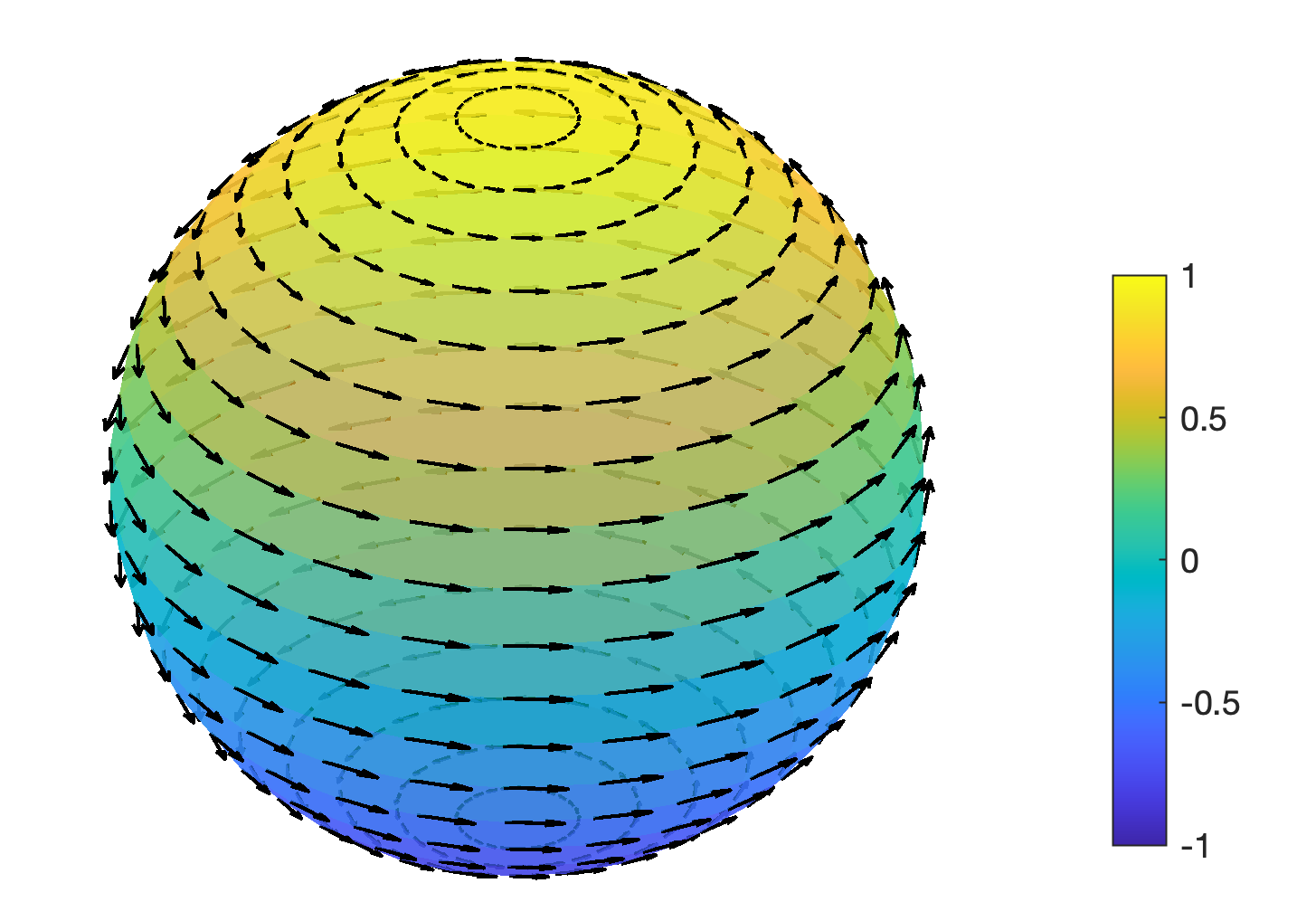
It is helpful to express this stationary flow using spherical coordinates, for which and
| (63) |
The modulus of the vortex velocity field is
| (64) |
which vanishes at the poles and reaches the maximum at the equator (see Fig. 1). Since and , we have . The vorticity of the vortex fluid reads
| (65) |
and the correction is . Due to compactness of the sphere, , the vorticity of this vortex flow has the profile of a vortex-dipole. It is worthwhile mentioning that the vortex flows we found here are analogous to zonal Rossby–Haurwitz flows in Euler fluids on a sphere Tritton (2012); Nualart (2023), which play an important role in analyzing dynamics of atmosphere of Earth Rossby (1939); Platzman (1968); Haurwitz (1940).
VI Conclusion
We generalize the vortex fluid theory on a plane to closed surfaces with zero genus. The dynamical equation is derived using the minimal coupling principle from it on a flat surface. An additional curvature term emerges and describes the interaction between topological defects and curvature in the hydrodynamical level. Since the vortex fluid equation contains second derivatives of vectors, there is an ambiguity for applying the minimal coupling principle directly. Our method does get over this difficulty and provides a feasible recipe to investigate other complex fluids on curved surfaces. For a sphere, a nontrivial stationary vortex flow is found analytically. It poses a challenge to find analytic solutions for surfaces with non-constant Gaussian curvature. For surfaces with Gaussian curvature weakly depending on positions [ with ], it might be possible to treat as perturbations and investigate the effects of non-constant Gaussian curvature. These are interesting topics which are worthwhile exploring in the feature.
The theory developed in this work leads to a broad understanding of the interaction between topological defects and curvature, and provides a theoretical framework for investigating rich phenomena involving a large number of quantum vortices Tononi et al. (2022); Kanai and Guo (2021); Li and Efimkin (2023); Saito and Hayashi (2023) in bubble trapped Bose-Einstein condensates Tononi et al. (2020); Tononi and Salasnich (2019).
Acknowledgment
We acknowledge J. Frauendiener, B. Feng, A. M. Mateo, L. A. Williamson, P. B. Blakie and A. S. Bradley for useful discussions. X.Y. acknowledges support from the National Natural Science Foundation of China (Grant No. 12175215), the National Key Research and Development Program of China (Grant No. 2022YFA 1405300) and NSAF (Grant No. U2330401).
References
- Son (2013) Dam Thanh Son, “Newton-cartan geometry and the quantum hall effect,” (2013), arXiv:1306.0638 [cond-mat.mes-hall] .
- Wiegmann (2013a) P. B. Wiegmann, “Hydrodynamics of euler incompressible fluid and the fractional quantum hall effect,” Phys. Rev. B 88, 241305 (2013a).
- Cho et al. (2014) Gil Young Cho, Yizhi You, and Eduardo Fradkin, “Geometry of fractional quantum hall fluids,” Phys. Rev. B 90, 115139 (2014).
- Gromov and Abanov (2014) Andrey Gromov and Alexander G. Abanov, “Density-curvature response and gravitational anomaly,” Phys. Rev. Lett. 113, 266802 (2014).
- Gromov et al. (2015) Andrey Gromov, Gil Young Cho, Yizhi You, Alexander G. Abanov, and Eduardo Fradkin, “Framing anomaly in the effective theory of the fractional quantum hall effect,” Phys. Rev. Lett. 114, 016805 (2015).
- Can et al. (2015) Tankut Can, Michael Laskin, and Paul B. Wiegmann, “Geometry of quantum hall states: Gravitational anomaly and transport coefficients,” Annals of Physics 362, 752–794 (2015).
- Mickelin et al. (2018) Oscar Mickelin, Jonasz Słomka, Keaton J. Burns, Daniel Lecoanet, Geoffrey M. Vasil, Luiz M. Faria, and Jörn Dunkel, “Anomalous chained turbulence in actively driven flows on spheres,” Phys. Rev. Lett. 120, 164503 (2018).
- Shankar et al. (2017) Suraj Shankar, Mark J. Bowick, and M. Cristina Marchetti, “Topological sound and flocking on curved surfaces,” Phys. Rev. X 7, 031039 (2017).
- Rank and Voigt (2021) M. Rank and A. Voigt, “Active flows on curved surfaces,” Physics of Fluids 33 (2021), 10.1063/5.0056099, 072110.
- Bogomolov (1977) VA Bogomolov, “Dynamics of vorticity at a sphere,” Fluid Dynamics 12, 863–870 (1977).
- Reuther and Voigt (2015) S. Reuther and A. Voigt, “The interplay of curvature and vortices in flow on curved surfaces,” Multiscale Modeling & Simulation 13, 632–643 (2015).
- Reuther and Voigt (2018) Sebastian Reuther and Axel Voigt, “Solving the incompressible surface Navier-Stokes equation by surface finite elements,” Physics of Fluids 30 (2018), 10.1063/1.5005142, 012107.
- Samavaki and Tuomela (2020) Maryam Samavaki and Jukka Tuomela, “Navier–stokes equations on riemannian manifolds,” Journal of Geometry and Physics 148, 103543 (2020).
- Sigurdsson and Atzberger (2016) Jon Karl Sigurdsson and Paul J. Atzberger, “Hydrodynamic coupling of particle inclusions embedded in curved lipid bilayer membranes,” Soft Matter 12, 6685–6707 (2016).
- Levine et al. (2004) Alex J. Levine, T. B. Liverpool, and F. C. MacKintosh, “Mobility of extended bodies in viscous films and membranes,” Phys. Rev. E 69, 021503 (2004).
- Rower et al. (2022) David A. Rower, Misha Padidar, and Paul J. Atzberger, “Surface fluctuating hydrodynamics methods for the drift-diffusion dynamics of particles and microstructures within curved fluid interfaces,” Journal of Computational Physics 455, 110994 (2022).
- Vitelli and Turner (2004) Vincenzo Vitelli and Ari M. Turner, “Anomalous coupling between topological defects and curvature,” Phys. Rev. Lett. 93, 215301 (2004).
- Turner et al. (2010) Ari M. Turner, Vincenzo Vitelli, and David R. Nelson, “Vortices on curved surfaces,” Rev. Mod. Phys. 82, 1301–1348 (2010).
- Aveline et al. (2020) David C Aveline, Jason R Williams, Ethan R Elliott, Chelsea Dutenhoffer, James R Kellogg, James M Kohel, Norman E Lay, Kamal Oudrhiri, Robert F Shotwell, Nan Yu, et al., “Observation of bose–einstein condensates in an earth-orbiting research lab,” Nature 582, 193–197 (2020).
- Carollo et al. (2022) Ryan A Carollo, David C Aveline, Brendan Rhyno, Smitha Vishveshwara, Courtney Lannert, Joseph D Murphree, Ethan R Elliott, Jason R Williams, Robert J Thompson, and Nathan Lundblad, “Observation of ultracold atomic bubbles in orbital microgravity,” Nature 606, 281–286 (2022).
- Bereta et al. (2021) Sálvio J. Bereta, Mônica A. Caracanhas, and Alexander L. Fetter, “Superfluid vortex dynamics on a spherical film,” Phys. Rev. A 103, 053306 (2021).
- Caracanhas et al. (2022) Mônica A. Caracanhas, Pietro Massignan, and Alexander L. Fetter, “Superfluid vortex dynamics on an ellipsoid and other surfaces of revolution,” Phys. Rev. A 105, 023307 (2022).
- Padavić et al. (2020) Karmela Padavić, Kuei Sun, Courtney Lannert, and Smitha Vishveshwara, “Vortex-antivortex physics in shell-shaped bose-einstein condensates,” Phys. Rev. A 102, 043305 (2020).
- Hally (1980) David Hally, “Stability of streets of vortices on surfaces of revolution with a reflection symmetry,” Journal of Mathematical Physics 21, 211–217 (1980).
- Kimura (1999) Y. Kimura, “Vortex motion on surfaces with constant curvature,” Proceedings of the Royal Society A: Mathematical, Physical and Engineering Sciences 455 (1999).
- Dritschel and Boatto (2015) David Gerard Dritschel and Stefanella Boatto, “The motion of point vortices on closed surfaces,” Proceedings of the Royal Society A: Mathematical, Physical and Engineering Sciences 471, 20140890 (2015).
- Wiegmann and Abanov (2014a) Paul Wiegmann and Alexander G. Abanov, “Anomalous hydrodynamics of two-dimensional vortex fluids,” Phys. Rev. Lett. 113, 034501 (2014a).
- Yu and Bradley (2017) Xiaoquan Yu and Ashton S. Bradley, “Emergent Non-Eulerian Hydrodynamics of Quantum Vortices in Two Dimensions,” Phys. Rev. Lett. 119, 185301 (2017).
- Stockdale et al. (2020) Oliver R. Stockdale, Matthew T. Reeves, Xiaoquan Yu, Guillaume Gauthier, Kwan Goddard-Lee, Warwick P. Bowen, Tyler W. Neely, and Matthew J. Davis, “Universal dynamics in the expansion of vortex clusters in a dissipative two-dimensional superfluid,” Phys. Rev. Res. 2, 033138 (2020).
- Wiegmann (2013b) P. B. Wiegmann, “Hydrodynamics of euler incompressible fluid and the fractional quantum hall effect,” Phys. Rev. B 88, 241305 (2013b).
- Doshi and Gromov (2021) Darshil Doshi and Andrey Gromov, “Vortices as fractons,” Communications Physics 4, 44 (2021).
- Grosvenor et al. (2021) Kevin T. Grosvenor, Carlos Hoyos, Francisco Peña Benitez, and Piotr Surówka, “Hydrodynamics of ideal fracton fluids,” Phys. Rev. Res. 3, 043186 (2021).
- Pitaevskii and Stringari (2016) Lev Pitaevskii and Sandro Stringari, Bose-Einstein Condensation and Superfluidity, Vol. 164 (Oxford University Press, 2016).
- Eyink and Sreenivasan (2006) Gregory L. Eyink and Katepalli R. Sreenivasan, “Onsager and the theory of hydrodynamic turbulence,” Rev. Mod. Phys. 78, 87–135 (2006).
- Onsager (1949) L. Onsager, “Statistical hydrodynamics,” Il Nuovo Cimento (1943-1954) 6, 279–287 (1949).
- Novikov (1975) EA Novikov, “Dynamics and statistics of a system of vortices,” Zhurnal Eksperimentalnoi i Teoreticheskoi Fiziki 68, 1868–1882 (1975).
- Aref et al. (1999) H Aref, PL Boyland, MA Stremler, and DL Vainchtein, “Turbulent statistical dynamics of a system of point vortices,” in Fundamental Problematic Issues in Turbulence (Springer, 1999) pp. 151–161.
- G.R.Kirchhoff (1876) G.R.Kirchhoff, in Vorlesungen über mathematische Physik (Teubner, Leipzig, 1876).
- Wiegmann and Abanov (2014b) Paul Wiegmann and Alexander G. Abanov, “Anomalous hydrodynamics of two-dimensional vortex fluids,” Phys. Rev. Lett. 113, 034501 (2014b).
- Avron (1998) JE Avron, “Odd viscosity,” Journal of statistical physics 92, 543–557 (1998).
- Fruchart et al. (2023) Michel Fruchart, Colin Scheibner, and Vincenzo Vitelli, “Odd viscosity and odd elasticity,” Annual Review of Condensed Matter Physics 14, 471–510 (2023).
- Avron et al. (1995) J. E. Avron, R. Seiler, and P. G. Zograf, “Viscosity of quantum hall fluids,” Phys. Rev. Lett. 75, 697–700 (1995).
- Hoyos and Son (2012) Carlos Hoyos and Dam Thanh Son, “Hall viscosity and electromagnetic response,” Phys. Rev. Lett. 108, 066805 (2012).
- Bradlyn et al. (2012) Barry Bradlyn, Moshe Goldstein, and N. Read, “Kubo formulas for viscosity: Hall viscosity, ward identities, and the relation with conductivity,” Phys. Rev. B 86, 245309 (2012).
- Abanov (2013) Alexander G Abanov, “On the effective hydrodynamics of the fractional quantum hall effect,” Journal of Physics A: Mathematical and Theoretical 46, 292001 (2013).
- Souslov et al. (2019) Anton Souslov, Kinjal Dasbiswas, Michel Fruchart, Suriyanarayanan Vaikuntanathan, and Vincenzo Vitelli, “Topological waves in fluids with odd viscosity,” Phys. Rev. Lett. 122, 128001 (2019).
- Banerjee et al. (2017) Debarghya Banerjee, Anton Souslov, Alexander G Abanov, and Vincenzo Vitelli, “Odd viscosity in chiral active fluids,” Nature communications 8, 1573 (2017).
- Lou et al. (2022) Xin Lou, Qing Yang, Yu Ding, Peng Liu, Ke Chen, Xin Zhou, Fangfu Ye, Rudolf Podgornik, and Mingcheng Yang, “Odd viscosity-induced hall-like transport of an active chiral fluid,” Proceedings of the National Academy of Sciences 119, e2201279119 (2022).
- Hoyos et al. (2014) Carlos Hoyos, Sergej Moroz, and Dam Thanh Son, “Effective theory of chiral two-dimensional superfluids,” Phys. Rev. B 89, 174507 (2014).
- Bogatskiy and Wiegmann (2019) A. Bogatskiy and P. Wiegmann, “Edge wave and boundary layer of vortex matter,” Phys. Rev. Lett. 122, 214505 (2019).
- Bogatskiy (2019) A Bogatskiy, “Vortex flows on closed surfaces,” Journal of Physics A: Mathematical and Theoretical 52, 475501 (2019).
- Moroz et al. (2018) Sergej Moroz, Carlos Hoyos, Claudio Benzoni, and Dam Thanh Son, “Effective field theory of a vortex lattice in a bosonic superfluid,” SciPost Phys. 5, 039 (2018).
- Ganeshan and Abanov (2017) Sriram Ganeshan and Alexander G. Abanov, “Odd viscosity in two-dimensional incompressible fluids,” Phys. Rev. Fluids 2, 094101 (2017).
- Monteiro and Ganeshan (2021) Gustavo M. Monteiro and Sriram Ganeshan, “Nonlinear shallow water dynamics with odd viscosity,” Phys. Rev. Fluids 6, L092401 (2021).
- Reeves et al. (2017) Matthew T. Reeves, Thomas P. Billam, Xiaoquan Yu, and Ashton S. Bradley, “Enstrophy cascade in decaying two-dimensional quantum turbulence,” Phys. Rev. Lett. 119, 184502 (2017).
- Reeves et al. (2014) Matthew T. Reeves, Thomas P. Billam, Brian P. Anderson, and Ashton S. Bradley, “Signatures of coherent vortex structures in a disordered two-dimensional quantum fluid,” Phys. Rev. A 89, 053631 (2014).
- Yu et al. (2016) Xiaoquan Yu, Thomas P. Billam, Jun Nian, Matthew T. Reeves, and Ashton S. Bradley, “Theory of the vortex-clustering transition in a confined two-dimensional quantum fluid,” Phys. Rev. A 94, 023602 (2016).
- Gauthier et al. (2019) Guillaume Gauthier, Matthew T. Reeves, Xiaoquan Yu, Ashton S. Bradley, Mark A. Baker, Thomas A. Bell, Halina Rubinsztein-Dunlop, Matthew J. Davis, and Tyler W. Neely, “Giant vortex clusters in a two-dimensional quantum fluid,” Science 364, 1264–1267 (2019).
- Billam et al. (2014) T. P. Billam, M. T. Reeves, B. P. Anderson, and A. S. Bradley, “Onsager-kraichnan condensation in decaying two-dimensional quantum turbulence,” Phys. Rev. Lett. 112, 145301 (2014).
- Skaugen and Angheluta (2016) Audun Skaugen and Luiza Angheluta, “Vortex clustering and universal scaling laws in two-dimensional quantum turbulence,” Phys. Rev. E 93, 032106 (2016).
- Chern (1955) Shing-Shen Chern, “An elementary proof of the existence of isothermal parameters on a surface,” Proceedings of the American Mathematical Society 6, 771–782 (1955).
- (62) Note that its integral over a closed surface vanishes, namely .
- Reall (2013) Harvey Reall, “Part 3 general relativity,” University of Cambridge 65 (2013).
- Gustafsson (2022) Björn Gustafsson, “Vortex pairs and dipoles on closed surfaces,” Journal of Nonlinear Science 32, 62 (2022).
- Marjieh et al. (2022) Raja Marjieh, Natalia Pinzani-Fokeeva, and Amos Yarom, “Enstrophy from symmetry,” SciPost Phys. 12, 085 (2022).
- Tritton (2012) David J Tritton, Physical fluid dynamics (Springer Science & Business Media, 2012).
- Nualart (2023) Marc Nualart, “On zonal steady solutions to the 2d euler equations on the rotating unit sphere,” (2023), arXiv:2201.05522 [math.AP] .
- Rossby (1939) Carl-Gustaf Rossby, “Relation between variations in the intensity of the zonal circulation of the atmosphere and the displacements of the semi-permanent centers of action,” J. mar. Res. 2, 38–55 (1939).
- Platzman (1968) George W Platzman, “The rossby wave,” Quarterly Journal of the Royal Meteorological Society 94, 225–248 (1968).
- Haurwitz (1940) Bernhard Haurwitz, “The motion of atmospheric disturbances on the spherical earth,” Journal of Marine Research 3, (3). (1940).
- Tononi et al. (2022) Andrea Tononi, Axel Pelster, and Luca Salasnich, “Topological superfluid transition in bubble-trapped condensates,” Phys. Rev. Research 4, 013122 (2022).
- Kanai and Guo (2021) Toshiaki Kanai and Wei Guo, “True mechanism of spontaneous order from turbulence in two-dimensional superfluid manifolds,” Phys. Rev. Lett. 127, 095301 (2021).
- Li and Efimkin (2023) Guangyao Li and Dmitry K. Efimkin, “Equatorial waves in rotating bubble-trapped superfluids,” Phys. Rev. A 107, 023319 (2023).
- Saito and Hayashi (2023) Hiroki Saito and Masazumi Hayashi, “Rossby–haurwitz wave in a rotating bubble-shaped bose–einstein condensate,” Journal of the Physical Society of Japan 92, 044003 (2023).
- Tononi et al. (2020) A. Tononi, F. Cinti, and L. Salasnich, “Quantum bubbles in microgravity,” Phys. Rev. Lett. 125, 010402 (2020).
- Tononi and Salasnich (2019) A. Tononi and L. Salasnich, “Bose-einstein condensation on the surface of a sphere,” Phys. Rev. Lett. 123, 160403 (2019).