Point and probabilistic forecast reconciliation for general linearly constrained multiple time series

Abstract

Forecast reconciliation is the post-forecasting process aimed to revise a set of incoherent base forecasts into coherent forecasts in line with given data structures. Most of the point and probabilistic regression-based forecast reconciliation results ground on the so called “structural representation” and on the related unconstrained generalized least squares reconciliation formula. However, the structural representation naturally applies to genuine hierarchical/grouped time series, where the top- and bottom-level variables are uniquely identified. When a general linearly constrained multiple time series is considered, the forecast reconciliation is naturally expressed according to a projection approach. While it is well known that the classic structural reconciliation formula is equivalent to its projection approach counterpart, so far it is not completely understood if and how a structural-like reconciliation formula may be derived for a general linearly constrained multiple time series. Such an expression would permit to extend reconciliation definitions, theorems and results in a straightforward manner. In this paper, we show that for general linearly constrained multiple time series it is possible to express the reconciliation formula according to a “structural-like” approach that keeps distinct free and constrained, instead of bottom and upper (aggregated), variables, establish the probabilistic forecast reconciliation framework, and apply these findings to obtain fully reconciled point and probabilistic forecasts for the aggregates of the Australian $GDP$ from income and expenditure sides, and for the European Area $GDP$ disaggregated by income, expenditure and output sides and by 19 countries.

• Linearly constrained multiple time series, Hierarchical/grouped time series,
  Point and probabilistic forecast reconciliation, Quarterly National Accounts, $GDP$

1 Introduction

Starting from Hyndman et al. (2011), regression-based forecast reconciliation has become an hot topic in the forecasting literature (van Erven & Cugliari, 2015; Wickramasuriya et al., 2019; Wickramasuriya, 2021; Panagiotelis et al., 2021; Jeon et al., 2019; Ben Taieb & Koo, 2019; Ben Taieb et al., 2021; Panagiotelis et al., 2023; Wickramasuriya, 2023). By forecast reconciliation, we mean a post-forecasting procedure (Di Fonzo & Girolimetto, 2023) in which previously (and however) generated incoherent predictions (called base forecasts) for all the components of a multiple time series are adjusted in order to fulfill some externally given linear constraints. These reconciled forecasts are said to be coherent. In many real world applications, forecasts of a large collection of time series have a natural organization according to a hierarchical structure. More precisely, a system is classified as hierarchical when series are created by aggregating others in a tree shape. When the system is formed by a unique tree, then the collection is called “hierarchical time series” (Hyndman et al., 2011). On the other side, when various hierarchies share the same series at both the most aggregated and disaggregated levels (top and bottom level, respectively), we face a “grouped time series” (Hyndman et al., 2016).

In the field of forecast reconciliation, the bottom-up and top-down approaches are among the earliest and best known ones. Bottom-up forecasting (Dunn et al., 1976) uses only forecasts at the bottom level to obtain all the reconciled forecasts. In contrast, top-down forecasting (Gross & Sohl, 1990) uses only the forecasts at the highest aggregated level. Having observed that neither forecasting approach uses all the available information, Hyndman et al. (2011) developed a regression-based reconciliation approach consisting in (i) forecasting all the series with no regard for the constraints, and (ii) using then a regression model to optimally combining these (base) forecasts in order to produce coherent forecasts. This approach has witnessed a continuous growth of the related literature (Hyndman et al., 2016; Athanasopoulos et al., 2020; Wickramasuriya, 2021; Panagiotelis et al., 2023), that in most cases grounds on the so-called structural representation of a hierarchical/grouped time series (Athanasopoulos et al., 2009), in which the variables are classified either bottom if they belong to the most disaggregated level, or upper if they are obtained by summing the lower levels’ variables. In mathematical terms, upper and bottom variables are linked by an aggregation matrix, which describes how the upper series are obtained from the bottom ones (Hyndman et al., 2011). This representation is directly related to the hierarchical structure, where the series are naturally classifiable and an aggregation matrix may be obtained with little effort. Theoretical aspects for point and probabilistic forecast reconciliation have been developed using a structural representation by Panagiotelis et al. (2021) and Panagiotelis et al. (2023), respectively (see also Wickramasuriya, 2021, 2023).

However, it can be shown (van Erven & Cugliari, 2015; Wickramasuriya et al., 2019; Bisaglia et al., 2020; Di Fonzo & Girolimetto, 2023) that reconciled forecasts may be obtained as the solution to a linearly constrained quadratic optimization problem, that does not require any “upper and bottom” classification of the involved variables. This approach grounds on a zero-constrained representation of the linearly constrained multiple time series (Di Fonzo & Girolimetto, 2023) describing the relationships linking all the individual series in the system. For a genuine hierarchical/grouped time series, where the top and bottom level variables are uniquely identified, it is easy to express the relationship between structural and zero-constrained representations. Wickramasuriya et al. (2019) show that the structural and the corresponding projection reconciliation approaches produce the same final reconciled forecasts. Unfortunately, given a zero-constrained representation of a linearly constrained multiple time series, finding the corresponding structural representation is not trivial (Di Fonzo & Girolimetto, 2023), and one of the objective of the present paper is to fill this gap.

Most of the forecast reconciliation approaches proposed in the literature refer to genuine hierarchical/grouped time series, that do not take into account the full spectrum of possible cases encountered in real-life situations. As pointed out by Panagiotelis et al. (2021), “concepts such as coherence and reconciliation (…) require the data to have only two important characteristics: the first is that they are multivariate, and the second is that they adhere to linear constraints”. Using a novel geometric interpretation, Panagiotelis et al. (2021) develop definitions and a formulation for linearly constrained multiple time series within a general framework and not just for simple summation hierarchical relationships. However, their results still ground on the structural representation valid only for genuine hierarchical/grouped time series, and this also holds for the probabilistic forecast reconciliation approach developed by Panagiotelis et al. (2023). Nevertheless, the point we wish to stress here is that when working with general linear constraints and many variables, the interchangeability between structural and zero-constrained representations, easy to recover for a genuine hierarchical/grouped time series, is no more always straightforward.

In this paper we address a number of open issues in point and probabilistic cross-sectional forecast reconciliation for general linearly constrained multiple time series. First, we introduce a general linearly constrained multiple time series by exploiting its analogies with an homogeneous linear system. Second, we show that the classical hierarchical representation for a multiple time series is a simple special case of the general representation. Third, we show that if it is possible to express a general linearly constrained multiple time series according to a “structural-like” representation, we can easily achieve the formulation for point and probabilistic regression-based reconciled forecasts using a linear combination matrix, with elements in $\mathbb{R}$, that is the natural extension of the aggregation matrix used in the structural reconciliation approach, with elements only in $\{0,1\}$. When the distinction between bottom and upper variables is no longer meaningful, we adopt a classification involving free and constrained variables, respectively, and show how to obtain a structural-like representation, possibly using well known linear algebra techniques, such as the Reduced Row Echelon Form and the QR decomposition (Golub & Van Loan, 1996, Meyer, 2000).

The remainder of the paper is structured as follows. In Section 2, we present the notation and the main results about the point forecast reconciliation for a genuine hierarchical/grouped time series and in the general case. We define the structural-like representation for a general linearly constrained multiple time series by distinguishing between free and constrained variables, instead of bottom and upper, and use this result in the probabilistic forecast reconciliation framework set out by Panagiotelis et al. (2023). In Section 3, we show how to obtain the linear combination matrix for the structural-like representation in a computationally efficient way. Two empirical applications are presented in Section 4. First, we extend the forecast reconciliation experiment for the Australian $GDP$ originally developed by Athanasopoulos et al. (2020) and Bisaglia et al. (2020), to obtain both point and probabilistic $GDP$ forecasts simultaneously coherent with their disaggregate counterpart forecasts from income and expenditure sides. Second, point and probabilistic forecasts are obtained for the European Area $GDP$ from income, expenditure and output sides, geographically disaggregated by 19 component countries, where the large number of series and constraints makes a full row rank zero-constraints matrix difficult to build. Section 5 contains conclusions.

2 Cross-sectional forecast reconciliation of a linearly constrained multiple time series

Let $\bm{x}_{t}$ be a $n$-dimensional linearly constrained multiple time series such that all the values for $t=1,...$ (either observed or not) lie in the coherent linear subspace $\mathcal{S}\in\mathbb{R}^{n}$, $\bm{x}_{t}\in\mathcal{S}\;\forall t>0$ (Panagiotelis et al., 2021), which means that all linear constraints are satisfied at time $t$. These constraints can be represented through linear equations and grouped as a (rectangular) linear system. Following Meyer (2000) and Leon (2015), let $x_{1,t},\dots,x_{n,t}$ be the observations of $n$ individual time series at a given time $t=1,...,T$. An homogeneous linear system of $p$ equations in the $n$ variables present in $\bm{x}_{t}$ can be written as

$$\left\{\begin{array}[]{ccccccccc}\gamma_{1,1}\;x_{1,t}&+&\gamma_{1,2}\;x_{2,t}&+&\dots&+&\gamma_{1,n}\;x_{n,t}&=&0\\ \vdots&\vdots&\vdots&\vdots&&\vdots&\vdots&\vdots&\vdots\\ \gamma_{p,1}\;x_{1,t}&+&\gamma_{p,2}\;x_{2,t}&+&\dots&+&\gamma_{p,n}\;x_{n,t}&=&0\\ \end{array}\right.,$$

where the $\gamma_{ij}$’s are real-valued coefficients. This system can be expressed in matrix form as

$$\bm{\Gamma}\bm{x}_{t}=\bm{0}_{(p\times 1)},$$ (1)

where $\bm{\Gamma}\in\mathbb{R}^{(p\times n)}$ is the coefficient matrix

$$\bm{\Gamma}=\begin{bmatrix}\gamma_{1,1}&\gamma_{1,2}&\dots&\gamma_{1,n}\\ \vdots&\vdots&\ddots&\vdots\\ \gamma_{p,1}&\gamma_{p,2}&\dots&\gamma_{p,n}\\ \end{bmatrix}.$$

Expression (1) is called “zero-constrained representation” of a linearly constrained multiple time series (Di Fonzo & Girolimetto, 2023).

2.1 Forecast reconciliation of a genuine hierarchical time series

Figure 1: A simple three-level hierarchical structure for a linearly constrained multiple time series

In Figure 1 it is shown a simple, genuine hierarchical time series (Athanasopoulos et al., 2009; Hyndman et al., 2011; Athanasopoulos et al., 2020; Hyndman & Athanasopoulos, 2021), that can be seen as a particular case of a linearly constrained multiple time series. This hierarchical structure is defined only by simple summation constraints,

$$\begin{array}[]{lcl}a_{1}&=&b_{1}+b_{2}+b_{3}+b_{4}+b_{5}\\ a_{2}&=&b_{1}+b_{2}\\ a_{3}&=&b_{3}+b_{4}+b_{5}\\ \end{array},$$ (2)

that can be easily transformed into a zero-constrained representation $\bm{\Gamma}\bm{x}=\bm{0}_{(8\times 1)}$, with $\bm{x}=\left[a_{1}\;a_{2}\;a_{3}\;b_{1}\;b_{2}\;b_{3}\;b_{4}\;b_{5}\;\right]^{\prime}=\left[\bm{a}^{\prime}\quad\bm{b}^{\prime}\right]^{\prime}$, and

$$\bm{\Gamma}=\left[\begin{array}[]{cccccccc}1&0&0&-1&-1&-1&-1&-1\\ 0&1&0&-1&-1&0&0&0\\ 0&0&1&0&0&-1&-1&-1\\ \end{array}\right]=\left[\bm{I}_{3}\quad-\bm{A}\right],$$

such as the $\gamma_{i,j}$’s coefficients are only -1, 0 and 1, and $\bm{a}=\bm{A}\bm{b}$.

In general, let $\bm{b}_{t}=\begin{bmatrix}b_{1,t}&\dots&b_{n_{b},t}\end{bmatrix}^{\prime}\in\mathbb{R}^{(n_{b}\times 1)}$ and $\bm{a}_{t}=\begin{bmatrix}a_{1,t}&\dots&a_{n_{a},t}\end{bmatrix}^{\prime}\in\mathbb{R}^{(n_{a}\times 1)}$, $t=1,...,T$, with $n=n_{a}+n_{b}$, be the $T$ vectors containing the bottom and the aggregated series, respectively, of a hierarchy. All series can be collected in the $T$ vectors

$$\bm{y}_{t}=\bm{P}\bm{x}_{t}=\begin{bmatrix}\bm{a}_{t}\\ \bm{b}_{t}\end{bmatrix}\in\mathbb{R}^{(n\times 1)},$$

where $\bm{P}\in\{0,1\}^{(n\times n)}$ is a permutation matrix used to appropriately re-order the original vector $\bm{x}_{t}$. If the classification as upper or bottom of the single time series in $\bm{x}_{t}$ is known in advance, we assume $\bm{x}_{t}=\bm{y}_{t}=\left[\bm{a}_{t}^{\prime}\quad\bm{b}_{t}^{\prime}\right]^{\prime}$, i.e. $\bm{P}=\bm{I}_{n}$ (no permutation of the original vector is needed). Moreover, also the linear combination (aggregation) matrix $\bm{A}\in\{0,1\}^{(n_{a}\times n_{b})}$ describing the summation constraints linking the upper time series to the bottom ones, $\bm{a}_{t}=\bm{A}\bm{b}_{t}$, is assumed known in advance. Thus the “structural representation” is simply given by (Athanasopoulos et al., 2009)

$$\bm{y}_{t}=\bm{S}\bm{b}_{t}\qquad\mbox{with}\qquad\bm{S}=\begin{bmatrix}\bm{A}\\ \bm{I}_{n_{b}}\end{bmatrix},$$ (3)

where $\bm{S}\in\{0,1\}^{(n\times n_{a})}$ is the structural (summation) matrix.

Suppose now we have the vector $\widehat{\bm{y}}_{h}=\begin{bmatrix}\widehat{\bm{a}}_{h}^{\prime}&\widehat{\bm{b}}_{h}^{\prime}\end{bmatrix}^{\prime}\in\mathbb{R}^{(n\times 1)}$ of unbiased and incoherent (i.e., $\widehat{\bm{y}}_{h}\neq\bm{S}\widehat{\bm{b}}_{h}$) base forecasts for the $n$ variables of the linearly constrained series $\bm{y}_{t}$ for the forecast horizon $h$. Hyndman et al. (2011) use the structural representation (3) to obtain the reconciled forecasts $\widetilde{\bm{y}}_{h}$ as

$$\widetilde{\bm{y}}_{h}=\bm{S}\bm{G}\widehat{\bm{y}}_{h},\quad\bm{G}=\left(\bm{S}^{\prime}\bm{W}^{-1}\bm{S}\right)^{-1}\bm{S}^{\prime}\bm{W}^{-1},$$ (4)

where $\bm{W}$ is a $(n\times n)$ p.d. matrix assumed known and $\widehat{\bm{y}}_{h}$ ($\widetilde{\bm{y}}_{h}$) is the vector containing the base (reconciled) forecasts at forecast horizon $h$. Some alternative matrices $\bm{W}$ have been proposed in the literature for the cross-sectional forecast reconciliation case:

• identity (ols): $\widehat{\bm{W}}_{\mathrm{ols}}=\bm{I}_{n}$ (Hyndman et al., 2011),

• series variance (wls): $\widehat{\bm{W}}_{\mathrm{wls}}=\bm{I}_{n}\odot\widehat{\bm{W}}_{\mathrm{sam}}$ (Hyndman et al., 2016),

• MinT-shr (shr): $\widehat{\bm{W}}_{\mathrm{shr}}=\widehat{\lambda}\widehat{\bm{W}}_{\mathrm{wls}}+(1-$ $\widehat{\lambda})\widehat{\bm{W}}_{\mathrm{sam}}$ (Wickramasuriya et al., 2019),

• MinT-sam (sam): $\widehat{\bm{W}}_{\mathrm{sam}}=\frac{1}{T}\sum_{t=1}^{T}\widehat{\bm{e}}_{t}\widehat{\bm{e}}_{t}^{\prime}$ is the covariance matrix of the one-step ahead in-sample forecast errors $\widehat{\mathbf{e}}_{t}$ (Wickramasuriya et al., 2019),

where the symbol $\odot$ denotes the Hadamard product, and $\widehat{\lambda}$ is an estimated shrinkage coefficient (Ledoit & Wolf, 2004).

The structural representation (3) may be transformed into the equivalent zero-constrained representation $\bm{a}_{t}-\bm{A}\bm{b}_{t}=\bm{0}_{(n_{a}\times 1)}$, that is (Wickramasuriya et al., 2019)

$$\bm{C}\bm{y}_{t}=\bm{0}_{(n_{a}\times 1)}\qquad\text{with}\qquad\bm{C}=\begin{bmatrix}\bm{I}_{n_{a}}&-\bm{A}\end{bmatrix}.$$ (5)

$\bm{C}\in\{-1,0,1\}^{(n_{a}\times n)}$ is a full row-rank zero constraints matrix used to obtain the point reconciled forecasts according to the projection approach (van Erven & Cugliari, 2015; Wickramasuriya et al., 2019; Di Fonzo & Girolimetto, 2023):

$$\widetilde{\bm{y}}_{h}=\bm{M}\widehat{\bm{y}}_{h},\quad\bm{M}=\bm{I}_{n}-\bm{W}\bm{C}^{\prime}\left(\bm{C}\bm{W}\bm{C}^{\prime}\right)^{-1}\bm{C}.$$ (6)

Structural and zero-constrained representations can be interchangeable depending on which of the two is more convenient to use, allowing for greater flexibility in the calculation of the reconciled forecasts. For, the zero-constrained representation appears to be less computational intensive: in equation (4) two matrices must be inverted, one of size ($n\times n$) and the other ($n_{b}\times n_{b}$), whereas only the inversion of an ($n_{a}\times n_{a}$) matrix is required in formula (6).

2.2 The general case: zero-constrained and structural-like representations

In the hierarchical/grouped cross-sectional forecast reconciliation there is a natural distinction between upper and bottom time series that leads to the construction of the matrix $\bm{C}$ as in (5), where the first $n_{a}$ columns refer to the upper and the remaining $n_{b}$ ($=n-n_{a}$) to the bottom variables, respectively. The time series in these two sets are categorized logically: all those related to the last level belong to the second group, the rest to the first. Most of the forecast reconciliation approaches proposed in the literature refer to genuine hierarchical/grouped time series and its structural representation. However, these do not take into account the full spectrum of possible cases encountered in real life situations. For a general linearly constrained multiple time series $\left(\bm{x}_{t},\;t=1,\ldots,T\right)$, the classification between upper and bottom variables might not be meaningful, prompting us rather to look for two new sets: the constrained variables, denoted as $\bm{c}_{t}\in\mathbb{R}^{(n_{c}\times 1)}$, and the free (unconstrained) variables, denoted as $\bm{u}_{t}\in\mathbb{R}^{(n_{u}\times 1)}$, with $n=n_{c}+n_{u}$, such that $\bm{y}_{t}=\bm{P}\bm{x}_{t}=\left[\bm{c}_{t}^{\prime}\quad\bm{u}_{t}^{\prime}\right]^{\prime}$, and

$$\bm{c}_{t}=\bm{A}\bm{u}_{t}.$$ (7)

In this general framework, $\bm{A}\in\mathbb{R}^{(n_{c}\times n_{u})}$ is the linear combination matrix associated to the linearly constrained multiple time series $\bm{x}_{t}=\bm{P}^{\prime}\bm{y}_{t}$, that can be thus expressed via the “structural-like representation”

$$\bm{y}_{t}=\bm{P}\bm{x}_{t}=\begin{bmatrix}\bm{c}_{t}\\ \bm{u}_{t}\end{bmatrix}=\bm{S}\bm{u}_{t}\quad\mathrm{with}\quad\bm{S}=\begin{bmatrix}\bm{A}\\ \bm{I}_{n_{u}}\end{bmatrix},$$ (8)

where $\bm{S}\in\mathbb{R}^{(n_{c}\times n_{u})}$ is the structural-like matrix. It is worth noting that a full-rank zero-constraints matrix $\bm{C}\in\mathbb{R}^{(n_{c}\times n)}$ like in expression (5) may be easily obtained by expression (8) and used for the full-rank zero constrained representation $\bm{C}\bm{y}_{t}=\bm{C}\bm{P}\bm{x}_{t}=\bm{0}_{(n_{c}\times 1)}$. Therefore, even for a general, possibly not genuine hierarchical/grouped, linearly constrained multiple time series, either the structural (4) or the projection (6) approaches may be used to perform the point forecast reconciliation of incoherent base forecasts.

$\;\;\bigcup\;$ $\qquad\longrightarrow\qquad$

Figure 2: A general linearly constrained structure: two hierarchies sharing only the same top-level series.

A simple example of a linearly constrained multiple time series that cannot be expressed as a genuine hierarchical/grouped structure is shown in Figure 2. In this case the variable X is at the top of two distinct hierarchies, that do not share the same bottom-level variables. The aggregation relationships between the upper variables X and A, and the bottom ones A1, A2, B, C, and D are given by:

$$\begin{aligned} X&=A1+A2+B\\ X&=C+D\\ A&=A1+A2\end{aligned}.$$ (9)

In this case, both the zero-constrained and the structural-like representations are found in a rather straightforward manner. We consider $\left\{A2,B,C,D\right\}$ as free variables, such that $\bm{y}_{t}=\bm{x}_{t}$ (i.e., $\bm{P}=\bm{I}_{4}$), with $\bm{c}_{t}=\begin{bmatrix}x_{{X},t}&x_{{A},t}&x_{{A1},t}\end{bmatrix}^{\prime}$ and $\bm{u}_{t}=\begin{bmatrix}x_{{A2},t}&x_{{B},t}&x_{{C},t}&x_{{D},t}\end{bmatrix}^{\prime}$. Thus, the coefficient matrix of the zero-constrained representation (1) is

$$\bm{\Gamma}=\begin{bmatrix}1&0&-1&-1&-1&0&0\\ 1&0&0&0&0&-1&-1\\ 0&1&-1&-1&0&0&0\\ \end{bmatrix}.$$

It is immediate to check that the system of linear constraints (9) may be re-written as

$$X =C+D$$

$$A =-B+C+D$$

$$A1 =-A2-B+C+D$$

that is $\bm{C}\bm{x}_{t}=\bm{0}_{(3\times 1)}$, where

$$\bm{C}=\begin{bmatrix}\bm{I}_{3}&-\bm{A}\end{bmatrix}=\begin{bmatrix}1&0&0&0&0&-1&-1\\ 0&1&0&0&1&-1&-1\\ 0&0&1&1&1&-1&-1\\ \end{bmatrix}\quad\mathrm{and}\quad\bm{A}=\begin{bmatrix}0&0&1&1\\ 0&-1&1&1\\ -1&-1&1&1\\ \end{bmatrix}.$$

The structural-like representation of the general linearly constrained multiple time series in Figure 2 is then $\bm{y}_{t}=\bm{S}\bm{u}_{t}$, with $\bm{S}=\left[\bm{A}^{\prime}\quad\bm{I}_{3}\right]^{\prime}$.

It should be mentioned, however, that for medium/large systems (with many constraints and/or variables), manually operating on the constraints could be time-consuming and challenging. In Section 3 we will show a general technique to derive the linear combination matrix $\bm{A}$ from a general zero-constraints matrix $\bm{\Gamma}$.

2.3 Probabilistic forecast reconciliation for general linearly constrained multiple time series

So far we have dealt with only point forecasting, but if one wishes to account for forecast uncertainty, probabilistic forecasts should be considered, as they - in the form of probability distributions over future quantities or events - measure the uncertainty in forecasts and are an important component of optimal decision making (Gneiting & Katzfuss, 2014).

Representation (8) states that $\bm{y}_{t}$ lies in an $n$-dimensional subspace of $\mathbb{R}^{n}$ spanned by the columns of $\bm{S}$, called “coherent subspace” and denoted by $\mathcal{S}$ (Panagiotelis et al., 2023). Now, let $\mathscr{F}_{\mathbb{R}^{n_{u}}}$ be the Borel $\sigma$-algebra on $\mathbb{R}^{n_{u}}$, $\left(\mathbb{R}^{n_{u}},\mathscr{F}_{\mathbb{R}^{n_{u}}},\nu\right)$ a probability space for the free variables, and ${s}:\mathbb{R}^{n_{u}}\rightarrow\mathbb{R}^{n}$ a continuous mapping matrix. Then a $\sigma$-algebra $\mathscr{F}_{\mathcal{S}}$ can be constructed from the collection of sets ${s}(\mathcal{B})$ for all $\mathcal{B}\in\mathscr{F}_{\mathbb{R}^{n}}$.

Definition 2.1 (Coherent probabilistic forecast for a linearly constrained multiple time series).

Given the triple $\left(\mathbb{R}^{n_{u}},\mathscr{F}_{\mathbb{R}^{n_{u}}},\nu\right)$, we define a coherent probability triple $\left(\mathcal{S},\mathscr{F}_{\mathcal{S}},\breve{\nu}\right)$ such that $\breve{\nu}({s}(\mathcal{B}))=\nu(\mathcal{B})$, $\forall\mathcal{B}\in\mathscr{F}_{\mathbb{R}^{n_{u}}}$.

In order to extend forecast reconciliation to the probabilistic setting, let $\left(\mathbb{R}^{n},\mathscr{F}_{\mathbb{R}^{n}},\widehat{\nu}\right)$ be a probability triple characterizing base (incoherent) probabilistic forecasts for all $n$ series, and let $\psi:\mathbb{R}^{n_{u}}\rightarrow\mathbb{R}^{n}$ be a continuous mapping function defined by Panagiotelis et al. (2023) as the composition of two transformations, ${s}\circ{g}$, where ${g}:\mathbb{R}^{n}\rightarrow\mathbb{R}^{n_{u}}$ is a continuous function corresponding to matrix ${\bm{G}}$ in equation (4).

Definition 2.2 (Probabilistic forecast reconciliation for a linearly constrained multiple time series).

The reconciled probability measure of $\widehat{\nu}$ with respect to $\psi$ is a probability measure $\widetilde{\nu}$ on $\mathcal{S}$ with $\sigma$-algebra $\mathscr{F}_{\mathcal{S}}$ such that

$$\widetilde{\nu}(\mathcal{A})=\widehat{\nu}\left(\psi^{-1}(\mathcal{A})\right),\quad\forall\mathcal{A}\in\mathscr{F}_{\mathcal{S}},$$ (10)

where $\psi^{-1}(\mathcal{A})=\left\{\bm{x}\in\mathbb{R}^{n}:\psi(\bm{x})\in\mathcal{A}\right\}$ is the pre-image of $\mathcal{A}$.

We consider two alternative approaches to deal with probabilistic forecast reconciliation according to the above definitions: a parametric framework, where probabilistic forecasts are produced under the assumption that the density function of the forecast errors is known, and a non-parametric framework, where no distributional assumption is made.

2.3.1 Parametric framework: Gaussian reconciliation

A reconciled probabilistic forecast may be obtained analytically for some parametric distributions, such as the multivariate normal (Yagli et al., 2020; Corani et al., 2021; Eckert et al., 2021; Panagiotelis et al., 2023; Wickramasuriya, 2023). In particular, if the base forecasts distribution is $\mathcal{N}(\widehat{\bm{y}}_{h},\bm{W}_{h})$, then the reconciled forecasts distribution is $\mathcal{N}(\widetilde{\bm{y}}_{h},\widetilde{\bm{W}}_{h})$, with

$$\widetilde{\bm{y}}_{h}={\bm{S}}\,{\bm{G}}\widehat{\bm{y}}_{h}\quad\mbox{and}\quad\widetilde{\bm{W}}_{h}={\bm{S}}\,{\bm{G}}\bm{W}_{h}{\bm{G}}^{\prime}\,{\bm{S}}^{\prime}.$$

The covariance matrix $\widetilde{\bm{W}}_{h}$ deserves special attention. In the simple case assumed by Wickramasuriya et al. (2019), $\bm{W}_{h}=k_{h}\bm{W}$, where $k_{h}$ is a proportionality constant, and the reconciled covariance matrix reduces to (see Appendix A):

$$\widetilde{\bm{W}}_{h}=k_{h}{\bm{S}}\,{\bm{G}}\bm{W}.$$ (11)

However, the proportionality assumption along the forecast horizons $h$ may be too restrictive, and computing $k_{h}$ cannot be an easy task. Thus, three alternative formulations of ${\bm{W}}_{h}$, already shown in Section 2.1, have been proposed in the forecast reconciliation literature:

• diagonal covariance matrix: $\bm{W}_{h}=\widehat{\bm{W}}_{\mathrm{wls}}$ (Corani et al., 2021; Panagiotelis et al., 2023);

• sample covariance matrix: $\bm{W}_{h}=\widehat{\bm{W}}_{\mathrm{sam}}$ (Panagiotelis et al., 2023);

• shrinkage covariance matrix: $\bm{W}_{h}=\widehat{\bm{W}}_{\mathrm{shr}}$ (Athanasopoulos et al., 2020).

2.3.2 Non-parametric framework: joint bootstrap-based reconciliation

When an analytical expression of the forecast distribution is either unavailable, or relies on unrealistic parametric assumptions, the empirical evaluation of the results may be grounded on reconciled samples (Jeon et al., 2019; Yang, 2020; Panagiotelis et al., 2023). At this end, we extend theorem 4.5 in Panagiotelis et al. (2023), originally formulated for genuine hierarchical/grouped time series, to the case of a general linearly constrained multiple time series. This theorem states that, if $\left(\widehat{\bm{y}}^{[1]},\ldots,\widehat{\bm{y}}^{[L]}\right)$ is a sample drawn from an incoherent probability measure $\widehat{\nu}$, then $\left(\widetilde{\bm{y}}^{[1]},\ldots,\widetilde{\bm{y}}^{[L]}\right)$, where $\widetilde{\bm{y}}^{[\ell]}:=\psi\left(\widehat{\bm{y}}^{[\ell]}\right)$ for $\ell=$ $1,\ldots,L\;$, is a sample drawn from the reconciled probability measure $\widetilde{\nu}$ as defined in (10). According to this result, reconciling each member of a sample obtained from an incoherent distribution yields a sample from the reconciled distribution. As a consequence, coherent probabilistic forecasts may be developed through a post-forecasting mechanism analogous to the point forecast reconciliation setting. For this purpose, the bootstrap procedure by Athanasopoulos et al. (2020) is applied:

1. appropriate univariate models $M_{i}$ for each series in the system are fitted based on the training data $\{y_{i,t}\}_{t=1}^{T}$, $i=1,\dots,n$, and the one-step-ahead in-sample forecast errors are stacked in an $(n\times T)$ matrix, $\widehat{\bm{E}}=\left\{\widehat{e}_{i,t}\right\}$;

2. $\widehat{\bm{y}}^{[l]}_{i,h}=f_{i}\left(M_{i},\widehat{e}_{i,h}^{[l]}\right)$ is computed for $h=1,\dots,H$ and $l=1,\dots,L$, where $f(\cdot)$ is a function of the fitted univariate model and its associated error, $\widehat{\bm{y}}^{[l]}_{i,h}$ is a sample path simulated for the $i-$th series, and $\widehat{e}_{i,h}^{[l]}$ is the $(i,h)-$th element of an $(n\times H)$ block bootstrap matrix containing $H$ consecutive columns randomly drawn from $\widehat{\bm{E}}$;

3. the optimal reconciliation formula, either according to the structural approach (4) or the projection approach (6), is applied to each $\widehat{\bm{y}}^{[l]}_{h}$.

3 Building the linear combination matrix $\mathbf{A}$

In the previous section, we limited ourselves to introduce the linear combination matrix $\bm{A}$ in expression (7), in line with the novel classification distinguishing between free (unconstrained) and constrained variables. In this section we propose two ways of building such a matrix in practice.

First, consider the simple case where there are no redundant constraints ($n_{c}=p$) and the first $n_{c}$ columns of $\bm{\Gamma}$ are linearly independent, so that $\bm{y}_{t}=\bm{x}_{t}=\Big{[}\bm{c}_{t}^{\prime}\quad\bm{u}_{t}^{\prime}\Big{]}^{\prime}$ and $\bm{\Gamma}\bm{y}_{t}=\bm{0}_{(n_{c}\times 1)}$. This homogeneous linear system can be written as

$$\bm{\Gamma}\bm{y}_{t}=\bm{0}_{(n_{c}\times 1)}\quad\Longleftrightarrow\quad\begin{bmatrix}\bm{\Gamma}_{c}&\bm{\Gamma}_{u}\end{bmatrix}\begin{bmatrix}\bm{c}_{t}\\ \bm{u}_{t}\end{bmatrix}=\bm{0}_{(n_{c}\times 1)},$$

where $\bm{\Gamma}_{c}\in\mathbb{R}^{(n_{c}\times n_{c})}$ contains the coefficients for the constrained variables, and $\bm{\Gamma}_{u}\in\mathbb{R}^{(n_{c}\times n_{u})}$ those for the free ones. Thanks to its non-singularity, $\bm{\Gamma}_{c}$ can be used to derive the equivalent zero-constrained representation:

$$\begin{bmatrix}\bm{I}_{n_{c}}&\left(\bm{\Gamma}_{c}\right)^{-1}\bm{\Gamma}_{u}\end{bmatrix}\begin{bmatrix}\bm{c}_{t}\\ \bm{u}_{t}\end{bmatrix}=\bm{C}\bm{y}_{t}=\bm{0}_{(n_{c}\times 1)},$$ (12)

where

$$\bm{C}=\begin{bmatrix}\bm{I}_{n_{c}}&-\bm{A}\end{bmatrix}\qquad\mathrm{and}\qquad\bm{A}=-\left(\bm{\Gamma}_{c}\right)^{-1}\bm{\Gamma}_{u}.$$ (13)

In practical situations, mostly if many variables and/or constraints are involved, categorizing variables as either constrained or free may be a challenging task: the goal is to identify a valid set of free variables with invertible coefficient matrix $\bm{\Gamma}_{c}$.

3.1 General (redundant) linear constraints framework

When $n$ is large, it is not always immediate to find a set of non-redundant constraints, so the method shown in expression (12) may be hardly applied in several real-life situations. We propose to overcome these issues by employing standard linear algebra tools, like the Reduced Row Echelon Form or the QR decomposition (Golub & Van Loan, 1996, Meyer, 2000), that are able to deal with redundant constraints and do not request any a priori classification of the single variables entering the multiple time series.

Reduced Row Echelon Form (rref)

A matrix is said to be in rref (Meyer, 2000) if and only if the following three conditions hold:

• it is in row echelon form;

• the pivot in each row is 1;

• all entries above each pivot are 0.

The idea is then very simple: classify as constrained the variables corresponding to the pivot positions of the rref representation coefficient matrix, while the remaining columns form the linear combination matrix $\bm{A}$. Usually a rref form is obtained through a Gauss-Jordan elimination (more details in Meyer, 2000). So, let $\bm{Z}\in\mathbb{R}^{(n_{c}\times n)}$ be the rref of $\bm{\Gamma}$ deprived of any possible null rows, then a permutation matrix $\bm{P}$ can be obtained starting from the pivot columns of $\bm{Z}$, such that

$$\bm{y}_{t}=\bm{P}\bm{x}_{t}=\begin{bmatrix}x_{\pi_{c}(1),t}&\dots&x_{\pi_{c}(n_{c}),t}&x_{\pi_{u}(1),t}&\dots&x_{\pi_{u}(n_{u}),t}\end{bmatrix},$$

where $\pi_{c}(i)$, $i=1,...,n_{c}$, is the position of the $i$-th pivot column (i.e., one of the columuns that identify the constrained variables) and $\pi_{u}(j)$, $j=1,...,n_{u}$, is the position of the $j$-th no-pivot column (i.e., one of the columns associated to the free variables). Then, the linear combination matrix $\bm{A}$ can be extracted from the expression

$$\bm{C}=\bm{Z}\bm{P}^{\prime}=\begin{bmatrix}\bm{I}_{n_{c}}&-\bm{A}\end{bmatrix}.$$

Additional examples can be found in the online appendix.

QR decomposition

Given the $(p\times n)$ coefficient matrix $\bm{\Gamma}$ of the zero-constrained representation (1), $\bm{\Gamma}=\bm{Q}\bm{R}\bm{P}$ is a QR decomposition with column pivoting (Lyche, 2020), where $\bm{Q}\in\mathbb{R}^{(p\times p)}$ is a square and orthonormal matrix ($\bm{Q}^{\prime}\bm{Q}=\bm{Q}\bm{Q}^{\prime}=\bm{I}_{p}$), $\bm{P}\in\{0,1\}^{(n\times n)}$ is a permutation matrix, and $\bm{R}\in\mathbb{R}^{(p\times n)}$ is an upper trapezoidal matrix (Anderson et al., 1992, 1999) such that

$$\bm{R}=\begin{cases}\big{[}\bm{R}_{c}\quad\bm{R}_{u}\big{]}&\mbox{if}\;\bm{\Gamma}\;\mbox{is full-rank}\\[2.84544pt] \begin{bmatrix}\bm{R}_{c}&\bm{R}_{u}\\ \bm{0}_{[(p-n_{c})\times n_{c}]}&\bm{0}_{[(p-n_{c})\times n_{u}]}\end{bmatrix}&\mbox{if}\;\bm{\Gamma}\;\mbox{is not full-rank}\end{cases},$$

where $\bm{R}_{c}\in\mathbb{R}^{(n_{c}\times n_{c})}$ is upper triangular, and $\bm{R}_{u}\in\mathbb{R}^{(n_{c}\times n_{u})}$ is nonsingular (Golub & Van Loan, 1996). Applying this decomposition to the homogenous system (1), we obtain

$$\bm{\Gamma}\bm{x}_{t}=\bm{Q}\bm{R}\bm{P}\bm{x}_{t}=\bm{Q}\bm{R}\bm{y}_{t}=\bm{0}_{(p\times 1)},$$

that is equivalent to (Meyer, 2000)

$$\begin{cases}\bm{Q}\bm{z}=\bm{0}_{(p\times 1)}\\ \bm{R}\bm{y}_{t}=\bm{z}=\bm{0}_{(p\times 1)}\end{cases}.$$

Due to the non-singularity of $\bm{Q}$, $\bm{z}=\bm{0}_{(p\times 1)}$ is the unique solution to the homogenous system $\bm{Q}\bm{x}=\bm{0}_{(p\times 1)}$ (Lyche, 2020). Then, the homogeneous system (1) representing a general linearly constrained time series may be re-written as $\big{[}\bm{R}_{c}\quad\bm{R}_{u}\big{]}\bm{y}_{t}=\bm{0}_{(n_{c}\times 1)}$. Finally, from (12) we obtain

$$\bm{C}=\big{[}\bm{I}_{n_{c}}\quad-\bm{A}\big{]}\qquad\mathrm{and}\qquad\bm{A}=-\bm{R}_{c}^{-1}\bm{R}_{u},$$

where $\bm{R}_{c}$ is invertible by construction (Golub & Van Loan, 1996). It is worth noting that the Pivoted QR decomposition generates a permutation matrix $\bm{P}$ that “moves” the free variables in $\bm{x}_{t}$ to the bottom part of the re-ordered vector $\bm{y}_{t}$, that is $\bm{P}\bm{x}_{t}=\bm{y}_{t}=\big{[}\bm{c}_{t}^{\prime}\quad\bm{u}_{t}^{\prime}\big{]}^{\prime}$.

It should be noted that in both cases (QR and rref), $\bm{P}=\bm{I}_{n}$ if the first $n_{c}$ columns of $\bm{\Gamma}$ are linearly independent. This means that both algorithms start by assuming as constrained and free the variables as they appear in $\bm{x}$, whose ordering is then changed only if it is not feasible for the constraints operating on the multivariate time series in equation (1).

4 Empirical applications

In this section we present two macroeconomics applications involving general linearly constrained multiple time series which do not have a genuine hierarchical/grouped structure. In the first case, in the wake of Athanasopoulos et al. (2020), we forecast the Australian $GDP$ from income and expenditure sides, for which Bisaglia et al. (2020) already provided a full row-rank $\bm{C}$ matrix. The second application concerns the European $GDP$ disaggregated by three sides (income, expenditure and output) and 19 member countries. In this case, building a full row-rank zero constraints matrix is not an easy task, so we use a QR decomposition (Section 3.1). Detailed informations on the variables in either dataset are reported in the online appendix.

4.1 Reconciled probabilistic forecasts of the Australian $GDP$ from income and expenditure sides

Athanasopoulos et al. (2020) first considered the reconciliation of point and probabilistic forecasts of the 95 Australian Quarterly National Accounts (QNA) variables that describe the Gross Domestic Product ($GDP$) at current prices from the income and expenditure sides, interpreted as two distinct hierarchies. In the former case (income), $GDP$ is the top level aggregate of a hierarchy of 15 lower level aggregates with $n_{a}^{I}=6$ and $n_{b}^{I}=10$, whereas in the latter (expenditure), $GDP$ is the top level aggregate of a hierarchy of 79 time series, with $n_{a}^{E}=27$ and $n_{b}^{E}=53$ (for details, Athanasopoulos et al., 2020; Bisaglia et al., 2020; Di Fonzo & Girolimetto, 2022, 2023).

Considering these two hierarchies as distinct yields different $GDP$ forecasts depending on the considered disaggregation (either by income or expenditure). The fact that the two hierarchical structures describing the National Accounts share only the same top-level series ($GDP$), prevents the adoption for the whole set of $n=95$ distinct variables of the original structural reconciliation approach proposed by Hyndman et al. (2011). However, it is possible to use the results shown so far for a general linearly constrained multiple time series. The homogeneous constraints valid for the variables are described by the following $(33\times 95)$ matrix $\bm{\Gamma}$ (Bisaglia et al., 2020):

$$\bm{\Gamma}=\begin{bmatrix}1&\bm{0}_{5}^{\prime}&-{\bf 1}_{10}^{\prime}&\bm{0}_{26}^{\prime}&\bm{0}_{53}^{\prime}\\ 1&\bm{0}_{5}^{\prime}&\bm{0}_{10}^{\prime}&\bm{0}_{26}^{\prime}&-{\bf 1}_{53}^{\prime}\\ \bm{0}_{5}&{\bf I}_{5}&-\bm{A}^{I}&\bm{0}_{5\times 26}&\bm{0}_{5\times 53}\\ \bm{0}_{26}&\bm{0}_{26\times 5}&\bm{0}_{26\times 10}&{\bf I}_{26}&-\bm{A}^{E}\end{bmatrix},$$ (14)

where $\bm{A}^{I}\in\{0,1\}^{(5\times 10)}$ and $\bm{A}^{E}\in\{0,1\}^{(26\times 53)}$ are the aggregation matrices for the income and the expenditure sides, respectively, and $\bm{\Gamma}$ has already full row-rank. A structural-like representation of the multiple time series that incorporates both sides’ accounting constraints may be obtained by transforming $\bm{\Gamma}$ through, for example, the QR technique described in Section 3.1. This operation results in a $(33\times 95)$ matrix $\bm{C}=\left[\bm{I}_{33}\;-\bm{A}\right]$, where $\bm{A}$ is the $(33\times 62)$ linear combination matrix shown in Figure 3, and $\bm{S}=\left[\bm{A}^{\prime}\quad\bm{I}_{62}\right]^{\prime}$ is the structural-like matrix (see Section 2.2).

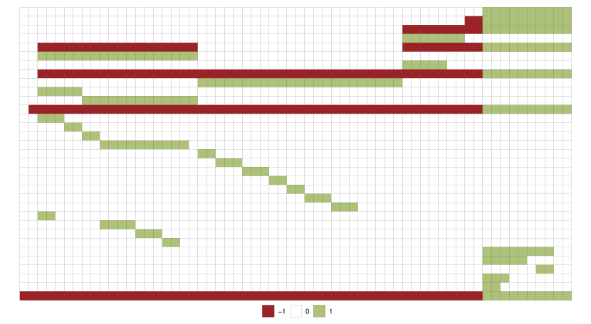
Figure 3: Linear combination matrix $\bm{A}$ for the Australian $GDP$ from income and expenditure sides.

We perform a forecasting experiment as the one designed by Athanasopoulos et al. (2020). Base forecasts from $h=1$ quarter ahead up to $h=4$ quarters ahead for all the 95 separate time series have been obtained through simple univariate ARIMA models selected using the auto.arima function of the R-package forecast (Hyndman & Khandakar, 2008). The first training sample is set from 1984:Q4 to 1994:Q3, and a recursive training sample with expanding window length is used, for a total of 94 forecast origins. Finally the reconciled forecasts are obtained using three reconciliation approaches (ols, wls and shr, see Section 2.1) through the R package Foreco (Girolimetto & Di Fonzo, 2023).

In Athanasopoulos et al. (2020) the probabilistic forecasts of the Australian quarterly $GDP$ aggregates are separately reconciled from income $\big{(}\widetilde{X}_{GDP}^{I}\big{)}$ and expenditure $\big{(}\widetilde{X}_{GDP}^{E}\big{)}$ sides. This means that the empirical forecast distributions $\widetilde{X}_{GDP}^{I}$ and $\widetilde{X}_{GDP}^{E}$ are each coherent (see Section 2.3) within its own pertaining side with the other empirical forecast distributions, but in general $\widetilde{X}_{GDP}^{I}\neq\widetilde{X}_{GDP}^{E}$ at any forecast horizon. This circumstance could confuse the user, mostly when the difference between the empirical forecast distributions is not negligible, as shown in Figure 4, where the $GDP$ empirical forecast distributions from income and expenditure sides for 2018:Q1 are presented along with their fully reconciled counterparts through the shr joint bootstrap-based reconciliation approach (see subsubsection 2.3.2).

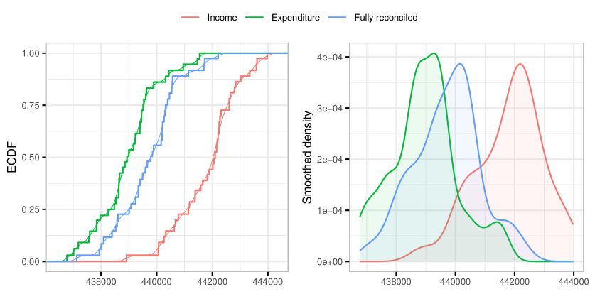
Figure 4: Australian $GDP$ empirical one-step-ahead forecast distributions for 2018:Q1, shr joint bootstrap-based reconciliation approach. Empirical Cumulative Distribution Function (left), and Smoothed density (right).

Point and probabilistic forecasting accuracy

To evaluate the accuracy of the point forecasts we use the Mean Square Error (MSE):

$$MSE_{j,h}=\frac{1}{nT_{h}}\sum_{i=1}^{n}\sum_{t=1}^{T_{h}}\tilde{e}_{i,j,t+h}^{\;2},$$

where $\tilde{e}_{i,j,t+h}=\left(\tilde{y}_{i,j,t+h}-{y}_{i,j,t+h}\right)$ is the the $h$-step-ahead forecast error using the approach $j$ to forecast the $i$-th series, $j=0$ denotes the base forecast (i.e., $\tilde{y}_{i,0,t+h}=\widehat{y}_{i,t+h}$), and $t$ is the forecast origin. To assess any improvement in the reconciled forecasts compared to the base ones, we use the $MSE$-skill score:

$$\left(1-\frac{MSE_{j,h}}{MSE_{0,h}}\right)\times 100.$$

The accuracy of the probabilistic forecasts is evaluated using the Cumulative Rank Probability Score (CRPS, Gneiting & Katzfuss, 2014):

$$\operatorname{CRPS}(\hat{P}_{i},z_{i})=\frac{1}{L}\sum_{l=1}^{L}\left|x_{i,l}-z_{i}\right|-\frac{1}{2L^{2}}\sum_{l=1}^{L}\sum_{j=1}^{L}\left|x_{i,l}-x_{i,j}\right|,\quad i=1,\dots,n,$$

where $\hat{P}_{i}(\omega)=\displaystyle\frac{1}{L}\displaystyle\sum_{l=1}^{L}\mathbf{1}\left(x_{i,l}\leq\omega\right)$, $\bm{x}_{1},\bm{x}_{2},\ldots,\bm{x}_{L}\in\mathbb{R}^{n}$ is a collection of $L$ random draws taken from the predictive distribution and $\bm{z}\in\mathbb{R}^{n}$ is the observation vector. In addition, to evaluate the forecasting accuracy for the whole system, we employ the Energy Score (ES), that is the CRPS extension to the multivariate case:

$$\operatorname{ES}(\hat{P},\bm{z})=\frac{1}{L}\sum_{l=1}^{L}\left\|\bm{x}_{l}-\bm{z}\right\|_{2}-\frac{1}{2(L-1)}\sum_{i=1}^{L-1}\left\|\bm{x}_{l}-\bm{x}_{l+1}\right\|_{2}.$$

Results

Table 1: MSE and CRPS-skill scores (relative to base forecasts) for the point and probabilistic Australian $GDP$ forecasts from alternative reconciliation approaches. Negative values are highlighted in red, the best for each row is marked in bold.

	Point forecasts			Probabilistic forecasts - CRPS(%)
	MSE (%)			Bootstrap			Gaussian
$h$	ols	wls	shr	ols	wls	shr	ols	wls	shr
Income
1	1.63	1.07	5.41	0.57	-1.26	0.52	0.13	-1.87	-0.45
2	2.54	5.68	6.10	1.46	0.68	-0.50	1.11	1.26	-0.34
3	2.28	7.81	4.56	0.18	-0.64	-1.93	0.14	-0.24	-1.69
4	1.98	9.33	7.04	-0.08	-1.12	-1.35	-0.23	-1.00	-1.39
Expenditure
1	4.53	0.07	2.48	1.10	0.78	0.08	0.64	-0.83	-0.70
2	5.09	3.90	1.72	2.34	1.25	-1.07	1.68	0.58	-1.95
3	6.96	9.18	6.24	2.42	1.50	-0.38	1.69	1.00	-1.02
4	8.01	11.76	8.34	3.73	2.73	0.72	3.18	2.49	0.20
Fully reconciled
1	4.59	1.14	4.77	1.13	-0.75	-0.20	-0.59	-3.46	-2.85
2	5.76	6.24	4.76	2.81	1.07	-1.27	1.30	-0.33	-3.02
3	7.31	10.94	8.21	1.99	0.26	-1.46	0.91	-0.62	-2.80
4	7.90	13.24	10.81	2.83	0.75	-0.63	1.86	-0.43	-2.05

Table 1 shows the MSE and CRPS-skill scores for the $GDP$ point and probabilistic reconciled forecasts. Table 2 presents the MSE and ES-skill scores for all 95 Australian QNA variables from both income and expenditure sides. The ‘Income’ and ‘Expenditure’ panels, respectively, reproduce the results found by Athanasopoulos et al. (2020). The ‘Fully reconciled’ panels show the skill scores for the simultaneously reconciled forecasts. For the point forecasts, all the reconciliation approaches improve forecast accuracy compared to the base forecasts. In detail, shr is almost always the best approach for the one-step-ahead forecasts, whereas wls is competitive for $h\geq 2$. Looking at the probabilistic reconciliation results in Table 1, it is worth noting that for $GDP$ ols outperforms both wls and shr, whatever side and framework (parametric or not) is considered. However, when all 95 variables are considered (Table 2), shr and wls approaches almost always show the best performance. In the Gaussian framework, these results are confirmed for the income side, whereas shr performs poorly when we look at the expenditure side (either fully reconciled or not).

Table 2: MSE and ES-skill scores (relative to base forecasts) for the point and probabilistic forecasts from alternative reconciliation approaches (all Australian QNA variables). Negative values are highlighted in red, the best for each row is marked in bold.

	Point forecasts			Probabilistic forecasts - ES(%)
	MSE (%)			Bootstrap			Gaussian
$h$	ols	wls	shr	ols	wls	shr	ols	wls	shr
Income
1	3.16	6.32	10.55	2.30	4.24	6.15	1.87	3.47	5.15
2	2.58	6.07	8.18	2.14	4.08	4.08	1.62	3.41	3.08
3	2.18	5.81	4.09	1.78	3.29	3.19	1.28	2.67	2.35
4	2.18	6.78	5.51	1.86	3.73	4.42	1.42	3.10	3.67
Income - Fully reconciled
1	3.78	7.57	8.85	2.77	4.58	4.87	1.30	1.94	2.25
2	2.91	6.12	6.92	2.59	3.95	3.40	1.20	1.59	0.87
3	2.67	6.23	5.57	2.24	3.70	3.17	0.92	1.60	0.79
4	2.87	7.21	6.07	2.65	4.40	3.95	1.44	2.34	1.59
Expenditure
1	6.50	6.75	8.78	3.71	4.54	4.94	2.20	1.92	2.58
2	4.90	5.50	5.52	2.88	3.04	2.68	1.28	0.67	0.32
3	4.27	6.08	5.65	2.57	2.94	2.29	0.88	0.71	0.09
4	4.01	6.69	5.20	2.43	2.65	1.63	0.77	0.44	-0.65
Expenditure - Fully reconciled
1	6.51	6.82	9.08	3.76	4.57	4.99	2.19	1.79	2.44
2	5.09	6.24	6.54	3.03	3.48	3.14	1.18	0.82	0.57
3	4.38	6.75	5.94	2.58	3.11	2.29	0.81	0.69	-0.12
4	3.98	7.33	5.82	2.36	2.82	1.81	0.60	0.32	-0.70

In Figure 5 are shown the results obtained by the non-parametric Friedman test and the post hoc “Multiple Comparison with the Best” (MCB) Nemenyi test (Koning et al., 2005; Kourentzes & Athanasopoulos, 2019; Makridakis et al., 2022) to determine if the forecasting performances of the different techniques are significantly different from one another. In general, wls always falls in the set of the best performing approaches. For the bootstrap-based probabilistic reconciled forecasts of the expenditure side variables, wls and shr significantly improves in terms of MSE and CRPS compared to the base forecasts. This result is confirmed in the remaining cases as well.

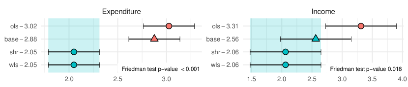
(a) Point forecasts (MSE)

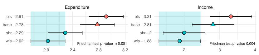
(b) Non parametric joint bootstrap probabilistic forecasts (CRPS)

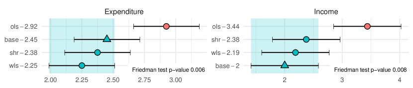
(c) Gaussian probabilistic forecasts (CRPS)

Figure 5: MCB Nemenyi test for the fully reconciled forecasts of the Australian QNA variables at any forecast horizon. In each panel, the Friedman test $p$-value is reported in the lower right corner. The mean rank of each approach is shown to the right of its name. Statistical differences in performance are indicated if the intervals of two forecast reconciliation approaches do not overlap. Thus, approaches that do not overlap with the blue interval are considered significantly worse than the best, and vice-versa.

In conclusion, when income and expenditure sides are simultaneously considered for both point and probabilistic forecasts, forecast reconciliation succeeds in improving the base forecasts of $GDP$ and its component aggregates, while preserving the full coherence with the National Accounts constraints.

4.2 Reconciled probabilistic forecasts of the European Area $GDP$ from output, income and expenditure sides

In this section, we consider the system of European QNA for the $GDP$ at current prices (in euro), with time series spanning the period 2000:Q1–2019:Q4. This system has many variables linked by several, possibly redundant, accounting constraints, such that it is difficult to manually build a system of non-redundant constraints.

The National Accounts are a coherent and consistent set of macroeconomic indicators that are used mostly for economic research and forecasting, policy design, and coordination mechanisms. In this dataset, $GDP$ is a key macroeconomic quantity that is measured using three main approaches, namely output (or production), income and expenditure. These parallel systems internally present a well-defined hierarchical structure of variables with relevant economic significance, such as Final consumption, on the expenditure side, Gross operating surplus and mixed income on the income side, and Total gross value added on the output side. In the EU countries, the data is processed on the basis of the ESA 2010 classification and are released by Eurostat. We consider the 19 Euro Area member countries (Austria, Belgium, Finland, France, Germany, Ireland, Italy, Luxembourg, Netherlands, Portugal, Spain, Greece, Slovenia, Cyprus, Malta, Slovakia, Estonia, Latvia, and Lithuania) that have been using the euro since 2015. In Figure 6 we have represented the aggregation matrices describing output, income, and expenditure constraints, respectively: in panel (a), matrix $\bm{A}_{\mathrm{O}}$ for the output side, in panel (b) matrix $\bm{A}_{\mathrm{I}}$ for the income side, and in panel (c) matrix $\bm{A}_{\mathrm{E}}$ for the expenditure side. The zero-constraints coefficient matrix describing the QNA variables for a single country can thus be written as

$$\bm{\Gamma}_{\mathrm{GDP}}=\begin{bmatrix}\bm{K}_{\mathrm{E}}&-\bm{A}_{\mathrm{E}}&\bm{0}_{(13\times 6)}&\bm{0}_{(13\times 3)}\\ \bm{K}_{\mathrm{I}}&\bm{0}_{(3\times 12)}&-\bm{A}_{\mathrm{I}}&\bm{0}_{(3\times 3)}\\ \bm{K}_{\mathrm{O}}&\bm{0}_{(1\times 12)}&\bm{0}_{(1\times 6)}&-\bm{A}_{\mathrm{O}}\\ \end{bmatrix},$$

where $\bm{K}_{\mathrm{E}}$, $\bm{K}_{\mathrm{I}}$ and $\bm{K}_{\mathrm{O}}$, respectively, are the following $(13\times 15)$, $(3\times 15)$ and $(1\times 15)$ matrices:

$$\bm{K}_{\mathrm{E}}=\begin{bmatrix}1&\bm{0}_{(1\times 12)}^{\prime}&\bm{0}_{(1\times 2)}^{\prime}\\ \bm{0}_{(12\times 1)}&\bm{I}_{12}&\bm{0}_{(12\times 2)}\\ \end{bmatrix},\;\bm{K}_{\mathrm{I}}=\begin{bmatrix}1&\bm{0}_{(1\times 12)}^{\prime}&\bm{0}_{(1\times 2)}^{\prime}\\ \bm{0}_{(2\times 1)}&\bm{0}_{(2\times 12)}&\bm{I}_{2}\\ \end{bmatrix},\;\bm{K}_{\mathrm{O}}=\begin{bmatrix}1&\bm{0}_{(1\times 14)}^{\prime}\end{bmatrix}.$$

This disaggregation is common for almost all European countries, the only differences being related to the presence/absence of an aggregate measuring the statistical discrepancy in each accounting side. The $(361\times 720)$ matrix describing the accounting relationships for the whole EA19 QNA by countries and accounting sides can be written as follows:

$$\bm{\Gamma}=\begin{bmatrix}\bm{\Gamma}_{\mathrm{GDP}}&\bm{0}_{(17\times 684)}\\ \left[\bm{0}_{(21\times 15)}\quad\bm{I}_{21}\right]&-\mathbf{1}_{19}^{\prime}\otimes\left[\bm{0}_{(21\times 15)}\quad\bm{I}_{21}\right]\\ \bm{0}_{(323\times 36)}&\bm{I}_{19}\otimes\bm{\Gamma}_{\mathrm{GDP}}\\ \end{bmatrix},$$

where $\otimes$ is the Kronecker product, and the top-left portion of $\bm{\Gamma}$ refers to the European Area aggregates as a whole. In order to proceed with the calculations, it is necessary to eliminate the columns related to null variables (e.g., the statistical discrepancy aggregate for the countries/sides where it is not contemplated, see footnote 11). Then, to eliminate possible remaining redundant constraints, we apply the QR decomposition (Section 3.1). Finally, we obtain the linear combination matrix $\bm{A}$, which refers to 311 free and 358 constrained time series, and the full rank zero-constraints matrix $\bm{C}=\begin{bmatrix}\bm{I}_{358}&-\bm{A}\end{bmatrix}$.

Figure 6: Linear combination matrices $\bm{A}$ for the European Area $GDP$: output side in panel (a), income side in panel (b), expenditure side in panel (c).

A rolling forecast experiment with expanding window is performed using ARIMA models to produce the individual series’ base forecasts. The first training set is set from 2000:Q1 to 2009:Q4, which gives 40 one-step-ahead, 39 two-step-ahead, 38 three-step-ahead and 37 four-step-ahead ARIMA forecasts, respectively. The used reconciliation approaches are ols, wls and shr, and the forecast accuracy is evaluated through MSE, CRPS and ES indices, as described in Section 4.1.

Table 3: MSE and ES-skill scores (relative to base forecasts) for the point and probabilistic forecasts from alternative reconciliation approaches (European Area QNA). Negative values are highlighted in red, the best for each row is marked in bold.

	Point forecasts			Probabilistic forecasts - ES(%)
	MSE (%)			Bootstrap			Gaussian
	ols	wls	shr	ols	wls	shr	ols	wls	shr
GDP	14.0	41.1	21.6	9.7	25.8	15.7	3.4	20.8	3.7
Sides
Expenditure	15.8	31.0	28.3	9.1	20.2	16.3	6.8	15.7	8.7
Income	-2.2	27.3	9.2	-0.3	15.3	5.6	-2.7	11.6	-3.2
Output	0.3	35.0	15.0	1.2	21.6	12.9	-1.5	17.1	1.3
Countries
EA19	17.6	37.1	31.6	10.1	23.5	18.1	7.8	19.3	10.0
Austria	$<$-30	18.5	21.5	-26.8	12.1	10.0	-21.6	9.1	5.4
Belgium	-5.9	13.5	21.0	-2.7	10.7	10.8	-3.1	8.3	5.9
Cyprus	$<$-30	11.7	8.6	$<$-30	7.1	1.7	$<$-30	3.6	-2.8
Estonia	$<$-30	20.9	26.8	$<$-30	12.7	11.2	$<$-30	9.7	6.7
Finland	$<$-30	24.8	14.7	$<$-30	15.3	9.5	$<$-30	13.2	3.4
France	4.4	19.1	-0.1	3.2	11.7	3.8	0.3	7.9	-6.8
Germany	15.0	20.6	25.0	13.5	21.6	18.6	7.5	11.1	6.8
Greece	$<$-30	1.5	$<$-30	-12.9	3.9	-7.1	-15.1	0.8	-14.1
Ireland	4.1	6.6	3.7	2.1	5.9	3.0	0.5	2.9	-0.7
Italy	9.8	12.6	24.0	8.4	10.8	17.1	4.4	4.9	7.8
Latvia	$<$-30	26.2	18.3	$<$-30	13.0	8.7	$<$-30	13.7	5.6
Lithuania	$<$-30	27.3	28.5	$<$-30	15.0	12.8	$<$-30	12.1	8.4
Luxembourg	$<$-30	6.6	-10.3	$<$-30	6.1	-3.0	$<$-30	2.0	-10.0
Malta	$<$-30	5.4	-9.9	$<$-30	4.9	-7.4	$<$-30	0.8	-12.0
Netherlands	7.4	16.9	11.9	6.1	14.1	7.3	3.5	11.7	4.4
Portugal	$<$-30	11.4	-8.1	$<$-30	7.4	-3.4	$<$-30	4.1	-10.1
Slovakia	$<$-30	21.5	16.4	$<$-30	10.0	6.9	$<$-30	9.2	2.0
Slovenia	$<$-30	24.1	15.5	$<$-30	13.5	8.3	$<$-30	11.1	1.8
Spain	6.5	17.7	0.9	5.3	9.2	1.4	1.7	6.4	-7.3

Results

Table 3 shows the MSE indices for point forecasts, and the ES indices for probabilistic nonparametric (bootstrap) and parametric (Gaussian) forecasts, respectively. The rows of the table are divided into three parts: the first row shows the results for $GDP$, the second to fourth rows the National Accounts’ divisions (income, expenditure, or output sides), while the remaining rows correspond to the 19 countries and EA19. All forecast horizons are considered.

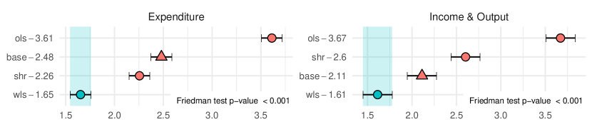
(a) Point forecasts

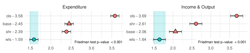
(b) Non parametric joint bootstrap probabilistic forecasts

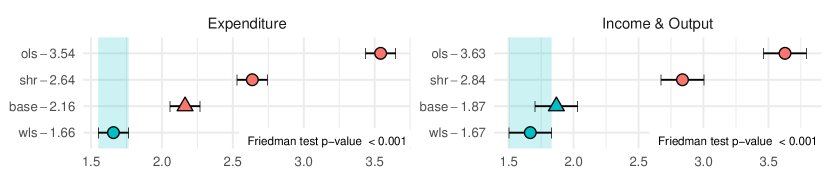
(c) Gaussian probabilistic forecasts

Figure 7: MCB Nemenyi test for the fully reconciled forecasts of the European Area QNA variables at any forecast horizon. In each panel, the Friedman test p-value is reported in the lower right corner. The mean rank of each approach is shown to the right of its name. Statistical differences in performance are indicated if the intervals of two forecast reconciliation approaches do not overlap. Thus, approaches that do not overlap with the blue interval are considered significantly worse than the best, and vice-versa.

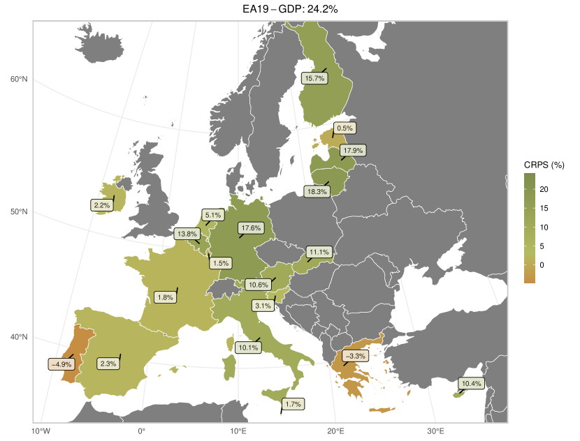
Figure 8: CRPS-skill scores of the one-step-ahead $GDP$ non-parametric joint bootstrap probabilistic reconciled (wls) forecasts for the 19 Euro Area countries.

When only $GDP$ is considered, any reconciliation approach consistently outperforms the base forecasts, both in the point and probabilistic cases. The wls approach confirms a good performance when we look at the income, expenditure, and output sides, while ols shows the worst performance. When the parametric framework is considered, shr is worse than the base forecast for the income side. At country level, ols is the approach that overall shows the worst performance, with many relative losses in the accuracy indices higher than 30%. It is worth noting that all reconciliation approaches always perform well for the whole Euro Area (EA19). Overall, in this forecasting experiment wls appears to be the most performing reconciliation approach, showing no negative skill score, and improvements higher than 20% and 10% for nonparametric and parametric probabilistic frameworks, respectively.

Figure 7 shows the MCB Nemenyi test at any forecast horizon, distinct by expenditure side and income and output sides, respectively. The results just seen are further confirmed by this alternative forecast assessment tool: it clearly appears that the wls approach almost always significantly improves compared to the base forecast, in terms of both point and probabilistic forecasts.

Finally, a visual evaluation of the accuracy improvement obtained through wls forecast reconciliation, although limited to a single forecast horizon, is offered by Figure 8, showing the European map with the CRPS skill scores for the one-step-ahead $GDP$ non-parametric probabilistic reconciled forecasts. It is worth noting that only for two countries (Greece and Portugal) a decrease is registered ($-3.3$% and $-4.9$%, respectively). In all other cases, improvements in the forecasting accuracy are obtained, with Germany and Lithuania leading the way with about 18%. Furthermore, the improvement in the forecasting accuracy for the $EA19-GDP$ is 24.2%, the highest throughout the whole Euro Area.

5 Conclusions

Producing and using coherent information, disaggregated by different characteristics useful for different decision levels, is an important task for any practitioner and quantitative-based decision process. At this end, in this article we aimed to generalize the results valid for the forecast reconciliation of a genuine hierarchical/grouped time series to the case of a general linearly constrained time series, where the distinction between upper and bottom variables, which is typical in the hierarchical setting, is no longer meaningful.

Two motivating examples have been considered, both coming from the National Accounts field, namely the forecast reconciliation of quarterly $GDP$ of (i) Australia, disaggregated by income and expenditure variables, and (ii) Euro Area 19, disaggregated by the income, output and expenditure side variables of 19 component countries. In both cases, the structure of the time series involved cannot be represented according to a genuinely hierarchical/grouped scheme, so the standard forecast reconciliation techniques fail in producing a “unique” $GDP$ forecast, either point or probabilistic, making it necessary to solve this annoying issue.

We have shown that using well known linear algebra tools, it is always possible to establish a formal connection between the unconstrained GLS structural approach originally developed by Hyndman et al. (2011), and the projection approach to reconciliation dating back to the work by Stone et al. (1942), and then applied to solve different reconciliation problems (Di Fonzo & Marini, 2011, van Erven & Cugliari, 2015, Wickramasuriya et al., 2019, Di Fonzo & Girolimetto, 2023). We propose a new classification of the variables forming the multiple time series as free and constrained, respectively, that can be seen as a generalization of the standard bottom/upper variables classification used in the hierarchical setting. Furthermore, we show techniques for deriving a linear combination matrix describing the relationships between these variables, starting from the coefficient matrix summarizing the (possible redundant) constraints linking the series.

The application of these findings to both point and probabilistic reconciliation techniques proved to be easy to implement and powerful, resulting in significant improvements in the forecasting accuracy of $GDP$ and its components in both forecasting experiments.

Appendix A Derivation of equation (11)

Denote $\bm{W}_{h}=k_{h}\bm{W}$, where $k_{h}$ is a proportionality constant and $\bm{W}$ is the p.d. covariance matrix used in the point forecast reconciliation formula (4). Then:

$$\widetilde{\bm{W}}_{h} =\bm{S}\bm{G}\bm{W}_{h}\bm{G}^{\prime}\bm{S}^{\prime}=k_{h}\bm{S}\bm{G}\bm{W}\bm{G}^{\prime}\bm{S}^{\prime}$$

$$=k_{h}\bm{S}\left(\bm{S}^{\prime}\bm{W}^{-1}\bm{S}\right)^{-1}\underbrace{\bm{S}^{\prime}\bm{W}^{-1}\bm{W}\bm{W}^{-1}\bm{S}\left(\bm{S}^{\prime}\bm{W}^{-1}\bm{S}\right)^{-1}}_{\bm{I}_{n}}\bm{S}^{\prime}$$

$$=k_{h}\bm{S}\left(\bm{S}^{\prime}\bm{W}^{-1}\bm{S}\right)^{-1}\bm{S}^{\prime}=k_{h}\bm{S}\underbrace{\left(\bm{S}^{\prime}\bm{W}^{-1}\bm{S}\right)^{-1}\bm{S}^{\prime}\bm{W}^{-1}}_{\bm{G}}\bm{W}=k_{h}\bm{S}\bm{G}\bm{W}.$$

References

- (1)
- Anderson et al. (1999) Anderson, E., Bai, Z., Bischof, C., Blackford, S., Demmel, J., Dongarra, J., Du Croz, J., Greenbaum, A., Hammerling, S., McKenney, A. & Others (1999), LAPACK Users’ Guide: Third Edition, Software, Environments, and Tools, Society for Industrial and Applied Mathematics.
- Anderson et al. (1992) Anderson, E., Bai, Z. & Dongarra, J. (1992), ‘Generalized QR factorization and its applications’, Linear Algebra and its Applications 162–164, 243–271.