Ergodicity breaking in rapidly rotating C60 fullerenes
Ergodicity, the central tenet of statistical mechanics, requires that an isolated system will explore all of its available phase space permitted by energetic and symmetry constraints. Mechanisms for violating ergodicity are of great interest for probing non-equilibrium matter and for protecting quantum coherence in complex systems. For decades, polyatomic molecules have served as an intriguing and challenging platform for probing ergodicity breaking in vibrational energy transport, particularly in the context of controlling chemical reactions. Here, we report the observation of rotational ergodicity breaking in an unprecedentedly large and symmetric molecule, 12C60. This is facilitated by the first ever observation of icosahedral ro-vibrational fine structure in any physical system, first predicted for 12C60 in 1986 (?). The ergodicity breaking exhibits several surprising features: first, there are multiple transitions between ergodic and non-ergodic regimes as the total angular momentum is increased, and second, they occur well below the traditional vibrational ergodicity threshold (?). These peculiar dynamics result from the molecules’ unique combination of symmetry, size, and rigidity, highlighting the potential of fullerenes to uncover emergent phenomena in mesoscopic quantum systems.
One Sentence Summary:
High-sensitivity infrared spectroscopy of the 1185 cm-1 spectral region in C60 reveals peculiar rotational dynamics of a large symmetric molecule.
Main Text:
Introduction. Isolated systems which break ergodicity have been explored in a variety of experimental settings, including spin glasses (?), ultracold neutral atoms (?, ?) and ions (?), and photonic crystals (?). These systems exhibit ergodicity breaking of spin configurations and momentum or spatial distributions. By contrast, gas phase polyatomic molecules provide opportunities to probe the ergodicity breaking of collective (rotational and vibrational) excitations in a finite quantum system. In this context, a topic of major interest has been the transport of energy deposited into molecular vibrations by optical pumping or collisions. Efficient intra-molecular vibrational redistribution (IVR) sets in once the vibrational energy exceeds a critical threshold defined by a combination of ro-vibrational coupling strengths and the density of states. (?, ?, ?, ?, ?). This vibrational ergodicity transition has been studied vigorously in the context of understanding and controlling unimolecular reaction dynamics (?).
Among polyatomic molecules, buckminsterfullerene (12C60) is notable for its structural rigidity and high degree of symmetry, which suppress IVR and allow for spectroscopic resolution (?) and optical pumping (?) of individual ro-vibrational states – an unusual and fortuitous situation for a molecule with 174 vibrational modes. Its small rotational constant and stiff cage-like structure ensure that hundreds of rotational states are populated even when vibrational excitations are largely frozen out, achievable with modest buffer gas cooling to K. Thus, a thermal ensemble of 12C60 can reveal extensive, state-resolved rotational perturbations spanning hundreds of rotational quanta by eliminating vibrational “hot bands”.
First observed and understood in atomic nuclei (?, ?, ?, ?, ?, ?, ?, ?), rotational perturbations can arise from spherical symmetry breaking in the frame fixed to a rotating self-bound deformable body (?), which lifts the degeneracy of different body-fixed projections of the total angular momentum vector J. Such perturbations, also called “tensor interactions” due to their anisotropic nature, manifest in fine-structure splitting of the total angular momentum () multiplets in rovibrational spectra and encode rich dynamics such as rotational bifurcations (?, ?), as previously observed in tetrahedral SnH4, CD4, CF4, SiH4, and SiF4 and octahedral SF6 molecules (?, ?, ?, ?, ?, ?, ?, ?, ?). Despite this, observing icosahedral tensor interactions, first predicted for 12C60 over three decades ago (?), has remained an elusive goal, since there are far fewer examples of icosahedral molecules, non-spherical interactions occur only at higher orders of interactions, and icosahedral molecules are necessarily larger than lower-symmetry spherical top molecules, implying a smaller rotational constant.
In this work, we observe these icosahedral tensor interaction splittings for the first time, revealing rotational ergodicity transitions in 12C60 at energies well below its IVR threshold (?). Specifically, as the molecule “spins up” to higher J, the dynamics of the angular momentum vector J in the molecule fixed frame switches between ergodic and non-ergodic regimes. In the non-ergodic regime, distinct J trajectories exist in the same energy range, but remain separated by energy barriers. In the limit of high , the tunnelling between these trajectories is too weak to restore ergodicity, leaving a characteristic signature in the fine-structure level statistics. This phenomenon differs from IVR in three key respects: (i) it involves the “transport” of the molecule frame orientation of J instead of vibrational energy, (ii) it can occur well below the IVR threshold, and (iii) it switches back and forth multiple times between ergodic (described by a 6th rank tensor interaction) and non-ergodic (described by a 10th rank tensor interaction) regimes as the angular momentum is varied. As we will show, this peculiar dynamical behaviour arises from multiple avoided crossings with other vibrational states, which induce non-monotonic variations in the molecule’s anisotropic character as is varied.
We describe the ro-vibrational structure of C60 with a general field-free molecular Hamiltonian
| (1) |
The scalar Hamiltonian contains only those combinations of J and vibrational angular momentum that preserve their spherical degeneracy (?),
| (2) |
where is the vibrational band origin, is the rotational constant, is the scalar centrifugal distortion constant, and is the Coriolis coupling constant.
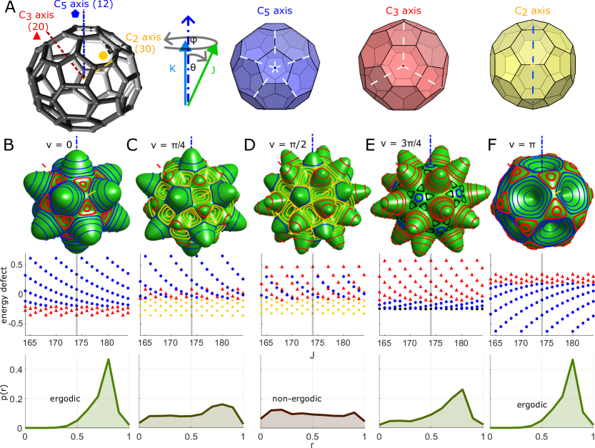
Ro-vibrational fine structure is encoded in the tensor Hamiltonian . For simplicity we consider a pure rotational tensor Hamiltonian consisting of the two lowest-order “icosahedral invariants”. These are linear combinations of spherical tensors of the same rank that transform according to the totally symmetric irreducible representation in the icosahedral point group (Ih) (?). They can be expressed (?) in the basis of spherical harmonics of degree and order , which depend explicitly on the molecular frame’s polar and azimuthal angles (Figure 1A). The first two nontrivial (anisotropic) icosahedral invariants, with ranks 6 and 10, are given by:
| (3) | ||||
| (4) |
from which we construct a truncated tensor Hamiltonian
| (5) |
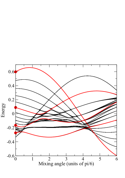
This Hamiltonian is parametrized by an overall scaling factor and mixing angle such that and correspond to pure and pure , respectively.
All operators that are incompatible with icosahedral point group symmetry, including any spherical harmonics of rank 1-5, 7-9, 11, 13, 14, … (?) vanish from the Hamiltonian. The use of full ro-vibrational tensor operators is unlikely to change the picture qualitatively, particularly when (approximately 100-300) is much greater than the vibrational angular momentum quantum number (?). These polyhedral invariants are similar to those used to describe the crystal field splitting of electronic orbitals due to an external lattice environment (?) or the ligand field splitting in transition metal complexes (?).
The energetic correction, or energy defect, associated with orienting J in different directions in the molecule frame, can be visualized by the altitude of a semi-classical “rotational energy surface” (RES), defined at a fixed . Various possible icosahedral RES’s, defined by their radii , corresponding to different mixing angles , are plotted for in the top panels of Figures 1B-F. Stationary points always lie on C2, C3, or C5 rotational symmetry axes. However, as varies, they change in character between minima, maxima, and saddle points. The RES dictates the dynamics of J in the molecule frame (?, ?, ?, ?, ?), analogous to how an adiabatic potential energy surface steers the relative motions of nuclei (?). During free evolution, the trajectory of J follows an equipotential contour of the RES.
In a full quantum mechanical treatment, the perturbation leads only to discrete energy defects given by the eigenvalues of in a fully symmetrized fixed- subspace. These orbits trace out the closed contours on the RES in Figure 1. The orbits may also be obtained directly from the RES: they are the trajectories which both (i) satisfy a Bohr quantization condition (?, ?), and (ii) transform according to the totally symmetric irreducible representation of the icosahedral point group (?). The latter condition accounts for the quantum indistinguishability of each bosonic nucleus in the 12C60 isotopologue (?, ?), and is analogous to the selection of odd or even rotational states in ortho- or para-hydrogen molecules, respectively. The energy defects are plotted for a range of in the center panels of Figures 1B-F and may be expected to appear in the ro-vibrational fine structure of 12C60.
In the preceding discussions, we have focused solely on the geometric effects of icosahedral symmetry. In general, however, the measured tensor defect spectra may exhibit additional -dependent scaling and offsets, which depend on intra-molecular couplings specific to 12C60. To extract all of these features, we now turn to the experimental measurements.
Methods-Experimental. To resolve ro-vibrational perturbations in 12C60, in this work we explored the P-branch region of the 1185 cm-1 T band, first identified as a region of potential interest in Ref. (?). Using cavity-enhanced continuous-wave (cw) spectroscopy with a quantum cascade laser (QCL) source, we achieved a minimum absorption sensitivity , or 1,000-fold better detection sensitivity per spectral element than in Ref (?) ( per comb mode). 600 MHz-wide absorption spectra were acquired by simultaneously scanning the QCL frequency and free spectral range of the enhancement cavity across molecular absorption lines, and recording the frequency-dependent absorption. These spectra were stitched together by a combination of direct calibration of the QCL frequency with a Fourier transform spectrometer, and comparison to matching spectral features in the broadband, low signal-to-noise (SNR) frequency comb spectrum of Ref (?). We obtain an absolute frequency accuracy of MHz throughout the entire measured frequency range, limited by the resolution of the reference frequency comb spectrum. Finally, to ensure consistency of the absorption signal over multiple days of data-taking, we have periodically re-measured the molecular absorption feature at R() at cm-1 and normalized all data taken around the same time to its line strength and measured cavity finesse.
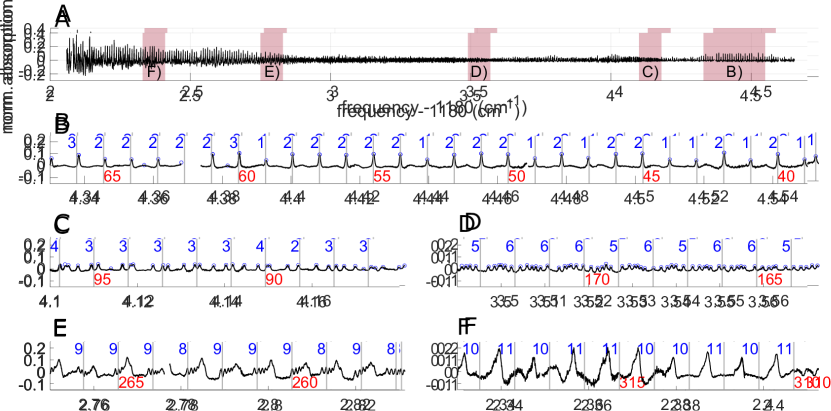
Methods - Analysis. The culmination of these efforts is the infrared spectrum in Figure 2, spanning the spectral region from 1182.0-1184.7 cm-1. At , there is a regular progression of rotational lines, similar to those in the R-branch (?). They rapidly split into intricate patterns before merging at and beyond . Zooming into the region labelled B), the rotational line centers can be fit to the scalar part of Equation 1, as was done in Ref (?).
| (6) |
where here refers to the ground-state total angular momentum. The scalar centrifugal distortion term is not significant at our spectral precision and range of . The fit yields = 0.0028 cm-1 for the ground state rotational constant, cm-1 for the excited state rotational constant, for the Coriolis coupling constant, and cm-1. Equation 6 yields a progression of rotational lines with a spacing of approximately , where . Note that the spectroscopic constants are under-determined and only serve to facilitate -assignment of the peaks in a manner consistent with the R-branch assignments of Ref (?). The extrapolated P-branch spectral line positions based on this scalar fit are plotted as gray vertical lines in Figure 2 B-F, with every fifth value labelled in red. The agreement with the measured line positions is excellent in the region where the spectrum appears unperturbed (Figure 2B).
To confirm our assignment, we compare the peak absorption cross sections to the nuclear spin weights of the ground state rotational levels and find that they match extremely well. Finally, we apply a frequency-dependent scaling factor to the raw absorption spectrum . This removes the effects of lab frame angular momentum degeneracy and the thermal ensemble, emphasizing the dynamics in the molecule fixed frame.
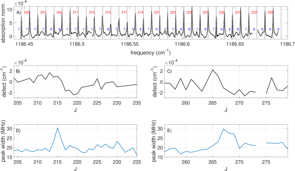
The peaks are identified manually and circled in blue. Figure 2C) and D) show two representative regions, at and , respectively, where peaks can still be individually resolved. The local peak density again matches the predicted nuclear spin weights (in blue), confirming that the ro-vibrational fine structure splitting originates from icosahedral tensor interactions of Equation 5 that lift -degeneracy. In Figures 2E) and F), we plot two regions where the peaks have begun to merge, and individual peaks can no longer be easily identified ().
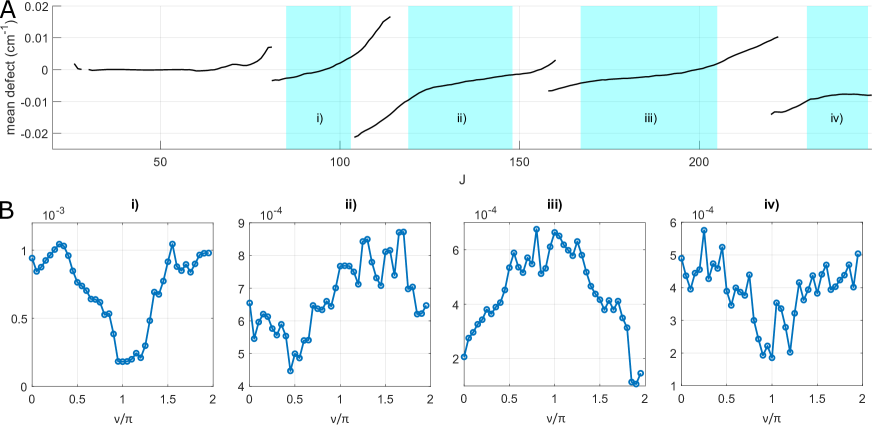
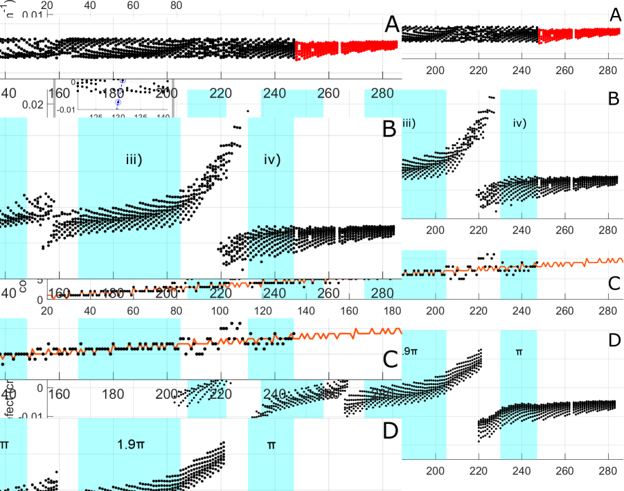
Interpreting the tensor splittings requires assigning each absorption peak to a particular . We begin by assigning each peak to its nearest value according to the scalar fit of Equation 6. Subtracting the scalar contribution (Equation 6) from the central frequency of each peak generates a single “period” of a Loomis-Wood-like defect plot in Figure 3A). There remains some ambiguity in the defect assignments, as illustrated in the inset of Figure 3A: each defect is constrained to the line with slope which passes through its current position.
By carefully rearranging individual defects according to these discrete allowed “moves”, we unwrap five distinct regions exhibiting continuous-looking patterns (Figure 3B). Because of the discontinuities at 80, 110, 160, and 220, there was still some ambiguity in the overall shift of the four perturbed sections labelled i)-iv). To remove this ambiguity, we recognized each section’s dominant pure-rank tensor character as follows: i) ; ii) ; iii) ; iv) . Eigenvalue spectra in Figures 1B), D), and F) show that the extremal eigenvalues associated with rotational symmetry axes occur when is an integer multiple of . The -assignment depicted in Figure 3B is one that satisfies this condition for all sections simultaneously. This final -assignment is confirmed by the excellent agreement between -resolved peak counts and calculated nuclear spin weight far from the discontinuities Figure 3C).
Results and Discussion. Having obtained a satisfactory -assignment of measured defects from the raw absorption spectrum, we now turn to its interpretation. We parametrize each of the four perturbed regions i)-iv) in Figure 3B) in terms of a mixed tensor (Equation 5), -dependent scaling , and -dependent scalar offset :
| (7) |
where are the -dependent tensor splittings as plotted in the lower panels of Figures 1B-F.
First, is obtained from the observed mean defect of each section. Next, by performing a point-cloud registration (?, ?, ?) to the theoretical eigenvalue spectra and the measured defect plot, we assign a best-fit mixing angle to each section: i) ; ii) 0.45; iii) 1.9, and iv) (?). Finally, is obtained from a least-squares fit to a polynomial in (?). The resulting reconstructed defect plot for regions i)-iv) is plotted in Figure 3D.
The abrupt changes in mixing angles are associated with transitions between ergodic and non-ergodic rotational dynamics as the molecule “spins up” to higher . We find that these dynamics transition from ergodic for region i), to non-ergodic for region ii), and back again for regions iv) and v).
The origin of this ergodicity breaking can be understood semi-classically using the RES’s in Figure 1 B), D), and F). The dynamics of are ergodic when time evolution explores the full space of symmetry-allowed states at the same energy. For region iii), the dominant tensor character is . Naively, the existence of 12 disconnected trajectories encircling the C5 axes breaks ergodicity. However, these trajectories cannot be distinguished in 12C60: due to the indistinguishability of the 12C nuclei, all 12 semi-classical trajectories correspond to a single quantum state given by their fully symmetric superposition. As such, the dynamics do explore the full range of states at a given energy, and hence is ergodic. The same argument applies for regions i) and iv), which differ from iii) only in the sign of energy defects (Figure 1F).
In contrast, for region ii) the dominant tensor character is . The C5 and C3 axes both correspond to peaks on the RES, and host trajectories over the same range of energies (Figure 3D). Trajectories encircling the C5 and C3 axes are distinguishable, and hence correspond to distinct quantum states. The quantum tunnelling between these trajectories is unable to restore the ergodicity: the tunnelling integral between C5 and C3 is exponentially small in (?, ?), whereas the level spacing only scales as . The scaling of the tunnelling integral follows from standard WKB results (?), while the level spacing can be seen from comparing the relatively fixed bandwidth of energy defects (Figure 3B) with the nuclear spin weight . Consequently, for our measured (well within the large- limit), tunnelling corrections are typically only perturbative.
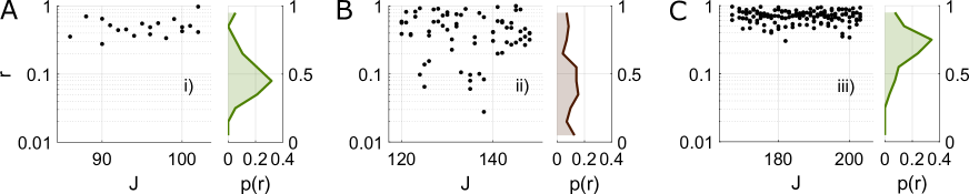
Level statistics provide a simple probe of this ergodicity breaking in molecular spectra (?, ?). Ergodic and non-ergodic dynamics are respectively associated with level repulsion and its absence (?). A useful diagnostic tool is the distribution , where is the ratio of consecutive level spacings (?, ?):
| (8) | ||||
| (9) |
In the limit of , level repulsion in an ergodic system causes , while for a non-ergodic system . Similar energy level statistics have been used to analyze systems as diverse as nuclear spectra (?) and ultra-cold atomic scattering (?), and many-body localization (?).
Figure 4A)-C) show the energy gap ratios computed from sections i)-iii), respectively, of the experimental defect plot (Figure 3B). Here, sections i) and iii) exhibit significant level repulsion characteristic of ergodicity, whereas section ii) does not, indicating non-ergodicity. We aggregate the energy gap ratios over each one of sections i)-iii) and their respective distributions in Figure 4D)-F). These distributions confirm the presence of level repulsion in sections i) and iii), and its absence in section ii).
We now turn from the dynamical interpretation of ro-vibrational defects to discuss their physical origin. Further analysis of Figure 3B reveals the defects arise from ro-vibrational coupling between the bright P-type excited T state and a background of perturbing dark states. Specifically, both the discontinuities and excess observed peaks at specific values are characteristic of avoided crossings with perturbing zero-order dark vibrational combination states. As they cross T from below, ro-vibrational coupling lifts the degeneracy of multiplets in the T state, imparting tensor character that depends on the identity of the perturbing vibrational state. The tensor character of the T state (specifically the fitted values) is stable in between avoided crossings, suggesting each of these sections is dominantly affected by just one perturbing state at a time. At the avoided crossings, this is expected to break down, as made particularly evident by the rapid change in mixing angle just before and after the avoided crossing at of Figure 3B. We note there is no apparent structure to the changes in mixing angle and coupling strength induced by the different avoided crossings, suggesting that the perturbing dark states are distinct, and not part of the same Coriolis manifold. Finally, using the observed density of perturbing states cm-1 and average measured vibrational coupling strength (bandwidth of the avoided crossings) of cm-1 (?), we arrive at an IVR threshold parameter (?) . Our 12C60 rotational ergodicity transitions are observed well below the IVR threshold, a conclusion supported by the spectroscopically well-resolved band.
Conclusion. For the first time, we have measured and characterized icosahedral tensor ro-vibrational coupling in 12C60. Analysis of the spectrum of ro-vibrational defects reveals that as the molecule is spun up to higher , there is a series of transitions in the dynamical behaviour of J in the fixed body frame. Specifically, J switches between ergodic and non-ergodic behaviour at particular values, leaving a characteristic imprint on the defect level statistics. These ergodicity transitions arise from dark vibrational combination states which cross the T state at particular values, transferring their anisotropic character onto the T state via ro-vibrational coupling.
Our measurements open the door to a rich hierarchy of emergent behaviour in C60 isotopologues, accessible at ever higher spectral resolution. The small nuclear spin-rotation interaction, for example in 13C substituted isotopologues of C60, can have a magnified effect due to the small superfine splittings near RES extrema. Such “hyperfine” coupling can lead to spontaneous symmetry breaking in a finite system (?, ?). These insights could prove useful for exploiting the exotic orientation state space of C60 for quantum information processing (?) and for investigating the quantum to classical transition of information spreading (?). Ultimately, spectroscopy of C60 isotopologues at ever higher spectral resolution promises to uncover deeper insights into the emergent dynamics of mesoscopic quantum many body systems.
References
- 1. W. G. Harter, D. E. Weeks, Chemical Physics Letters 132, 387 (1986).
- 2. D. E. Logan, P. G. Wolynes, The Journal of Chemical Physics 93, 4994 (1990).
- 3. K. Binder, A. P. Young, Reviews of Modern Physics 58, 801 (1986).
- 4. T. Kinoshita, T. Wenger, D. S. Weiss, Nature 440, 900 (2006).
- 5. M. Schreiber, et al., Science 349, 842 (2015).
- 6. J. Smith, et al., Nature Physics 12, 907 (2016).
- 7. M. Segev, Y. Silberberg, D. N. Christodoulides, Nature Photonics 7, 197 (2013).
- 8. G. M. Nathanson, G. M. Mcclelland, Journal of Chemical Physics 81, 629 (1984).
- 9. G. M. McClelland, G. M. Nathanson, J. H. Frederick, F. W. Farley, Intramolecular Vibration – Rotation Energy Transfer and the Orientational Dynamics of Molecules, vol. 7 (ACADEMIC PRESS, INC., 1988).
- 10. K. Sture, J. Nordholm, S. A. Rice, The Journal of Chemical Physics 61, 203 (1974).
- 11. D. M. Leitner, Entropy 20, 673 (2018).
- 12. D. J. Nesbitt, R. W. Field, Journal of Physical Chemistry 100, 12735 (1996).
- 13. P. B. Changala, M. L. Weichman, K. F. Lee, M. E. Fermann, J. Ye, Science 363, 49 (2019).
- 14. L. R. Liu, et al., PRX Quantum 3, 030332 (2022).
- 15. I. M. Pavlichenkov, Sov. Phys. JETP 55, 5 (1982).
- 16. I. M. Pavlichenkov, B. I. Zhilinskii, Annals of physics 184, 1 (1988).
- 17. Y. R. Shimizu, J. D. Garrett, R. A. Broglia, M. Gallardo, E. Vigezzi, Reviews of modern physics 61, 131 (1989).
- 18. I. M. Pavlichenkov, Physics Reports 226, 173 (1993).
- 19. S. Frauendorf, reviews of modern physics 73, 463 (2001).
- 20. H. Hübel, Progress in Particle and Nuclear Physics 54, 1 (2005).
- 21. J. Kvasil, R. G. Nazmitdinov, Physical Review C - Nuclear Physics 73, 014312 (2006).
- 22. J. Kvasil, R. G. Nazmitdinov, A. S. Sitdikov, P. Veselý, Physics of Atomic Nuclei 70, 1386 (2007).
- 23. K. Fox, H. W. Galbraith, B. J. Krohn, J. D. Louck, Physical Review A 15, 1363 (1977).
- 24. G. Pierre, D. A. Sadovskii, B. I. Zhilinskii, EUROPHYSICS LETTERS Europhys. Lett 10, 409 (1989).
- 25. R. S. Mcdowell, et al., Journal of Molecular Spectroscopy 83, 440 (1980).
- 26. C. W. Patterson’, A. S. Pine, Journal of Molecular Spectroscopy 96, 404 (1982).
- 27. J. P. Aldridge, et al., journal of molecular spectroscopy 58, 165 (1975).
- 28. K. C. Kim, W. B. Person, D. Seitz, B. J. Krohn, JOURNAL OF MOLECULAR SPECTROSCOPY 76, 322 (1979).
- 29. W. G. Harter, Journal of Statistical Physics 36, 749 (1984).
- 30. W. G. Harter, C. W. Patterson, Journal of Mathematical Physics 20, 1453 (1978).
- 31. W. G. Harter, H. P. Layer, F. R. Petersen, optics letters 4, 90 (1979).
- 32. R. S. Mcdowell, H. W. Galbraith, B. J. Krohn, C. D. Cantrell, Optics Communications 17, 178 (1976).
- 33. J. Bordé, C. J. Bordé, Chemical Physics 71, 417 (1982).
- 34. K. T. Hecht, Journal of Molecular Spectroscopy 5, 355 (1961).
- 35. Supplementary Information.
- 36. Y. Zheng, P. C. Doerschuk, Acta Crystallographica 52, 221 (1996).
- 37. P. R. Bunker, P. Jensen, Molecular Physics 97, 255 (1999).
- 38. K. R. Lea, M. J. Leask, W. P. Wolf, Journal of Physics and Chemistry of Solids 23, 1381 (1962).
- 39. B. J. S. Griffith, L. E. Orgel, Quarterly Reviews, Chemical Society 11, 381 (1957).
- 40. W. G. Harter, Physical Review A 24, 192 (1981).
- 41. W. G. Harter, C. W. Patterson, The Journal of Chemical Physics 80, 4241 (1984).
- 42. W. G. Harter, Computer Physics Reports 8, 319 (1988).
- 43. D. A. Sadovskii, B. I. Zhilinskii, J. P. Champion, G. Pierre, The Journal of Chemical Physics 92, 1523 (1990).
- 44. M. Khauss, Annual Review of Physical Chemistry 21, 39 (1970).
- 45. W. G. Harter, D. E. Weeks, The Journal of Chemical Physics 90, 4727 (1989).
- 46. R. D. Johnson, G. Meijer, D. S. Bethune, Journal of the American Chemical Society 112, 8983 (1990).
- 47. C. Yang, G. Medioni, Image and Vision Computing 10, 145 (1992).
- 48. P. J. Besl, N. D. Mckay, IEEE transactions on pattern analysis and machine intelligence 14, 239 (1992).
- 49. A. V. Segal, D. Haehnel, S. Thrun, Robotics: Science and Systems 5, 435 (2010).
- 50. A. Auerbach, Interacting electrons and Quantum magnetism (Springer Science+Business Media, 1994).
- 51. J. L. van Hemmen, A. Suto, Europhys. Lett 1, 481 (1986).
- 52. L. Landau, E. Lifshitz, Quantum Mechanics (Non-Relativistic Theory), vol. 3 (Pergamon Press, 1958).
- 53. R. L. Sundberg, E. Abramson, J. L. Kinsey, R. W. Field, The Journal of Chemical Physics 83, 466 (1985).
- 54. T. Zimmermann, H. Koppel, L. S. Cederbaum, G. Persch, W. Demtroder, Physical review letters 61, 3 (1988).
- 55. E. P. Wigner, SIAM review 9 (1967).
- 56. V. Oganesyan, D. A. Huse, Physical Review B - Condensed Matter and Materials Physics 75, 155111 (2007).
- 57. Y. Y. Atas, E. Bogomolny, O. Giraud, G. Roux, Physical Review Letters 110, 1 (2013).
- 58. A. Frisch, et al., Nature 507, 475 (2014).
- 59. D. A. Abanin, E. Altman, I. Bloch, M. Serbyn, Reviews of Modern Physics 91 (2019).
- 60. J. Bordé, et al., Physical Review Letters 45, 14 (1980).
- 61. V. V. Albert, J. P. Covey, J. Preskill, Physical Review X 10, 031050 (2020).
- 62. C. Zhang, P. G. Wolynes, M. Gruebele, Physical Review A 105, 1 (2022).
- 63. R. N. Zare, Angular momentum (Wiley-Interscience, 1988).
Acknowledgments:
This research was supported by AFOSR grant no. FA9550-19-1-0148; the National Science Foundation Quantum Leap Challenge Institutes (grant QLCI OMA-2016244); the National Science Foundation (grant Phys-1734006); the U.S. Department of Energy, Office of Science, National Quantum Information Science Research Centers, Quantum Systems Accelerator (QSA); and the National Institute of Standards and Technology. D.R. acknowledges support from the Israeli council for higher education quantum science fellowship, and is an awardee of the Weizmann Institute of Science – Israel National Postdoctoral Award Program for Advancing Women in Science. P.J.D.C. and N.Y.Y. acknowledge support from the AFOSR MURI program (FA9550-21-1-0069). T.T. acknowledges support from the NSF EPSCoR RII Track-4 Fellowship No. 1929190. We gratefully acknowledge comments on the manuscript from Aaron W. Young and Ya-Chu Chan.
Author Contributions: L.R.L, D. R., and J.Y. designed, discussed, and performed the experiment and analyzed the data. All authors participated in theory discussions and calculations, and writing of the paper.
Competing interests: The authors declare no competing interests.
Data Materials and Availability: All data are available in the main text, in the supplementary information, or through Harvard Dataverse. All materials requests and correspondence should be directed to Lee R. Liu or Jun Ye.
Supplementary Information
Materials and Methods
Supplementary Text
Tables S1 to S3
Figs. S1 to S4
References (28-50)
Materials and Methods.
Icosahedral invariant tensor operators
The full tensor part of the molecular Hamiltonian, including rotational and vibrational degrees of freedom, is given by
| (S1) |
where is the rank of the vibrational angular momentum operator, is the rank of the total angular momentum operator, and . The correlation between SO(3) and restricts the sum to (the terms with appear in the scalar part of the Hamiltonian). This is related to the allowed rotational states For simplicity, we will consider a pure rotational tensor Hamiltonian, i.e, which does not depend on vibrational angular momentum.
| (S2) |
Equation 7 provides some justification for why we have considered only pure rotational tensors; since we expect similar patterns of icosahedral splittings to appear in pure rotational or ro-vibrational manifolds (?), and the vibrational quantum number is constant throughout the excited state T manifold, we can absorb any vibrational dependence into the -dependent scaling factor (discussed more below).
Eigenvalues of and “A”-symmetry selection.
Here, we describe the procedure of calculating the eigenvalues of the mixed 6-th and 10-th rank tensor Hamiltonian (Equation 5) (?), where the 6-th and 10-th order icosahedral tensors are given by
| (S3) | ||||
| (S4) |
We obtain the matrix elements of these tensors by diagonalizing in the basis of symmetric top eigenstates where are the body-fixed and space-fixed projections of , respectively ( will be omitted in the following for notational simplicity). According to the Wigner-Eckart theorem, the matrix elements of can be factorized into a reduced matrix element which carries the dynamical content of the tensor operator and a component which only depends on geometry, expressed here in terms of Wigner 3-j symbols (?):
| (S7) | ||||
| (S12) |
for the rank tensor interaction and
| (S15) | ||||
| (S20) | ||||
| (S25) |
for the rank tensor interaction (note that the reduced matrix element used by Harter and Weeks (?) have been scaled by the factor to bring it into agreement with the convention of Ref. ?). Diagonalization yields possible eigenvalues, corresponding to the white contours on the RES of Figures 1B-F. To account for the quantum permutation statistics of the bosonic 12C nuclei comprising 12C60, we select only the eigenvalues belonging to totally symmetric eigenstates in Ih (?, ?). This reduces the number of fine-structure components, or the “nuclear spin weight”, to approximately .
In the following, we will set both of the reduced matrix elements to 1 to expose the mixing effects, as done by Harter and Weeks (?). It is important to keep in mind, however, that these matrix elements may scale differently with as , so the 10-th rank tensor contribution will become dominant at high .
To select the A symmetry species for the 6-th rank tensor spectrum of 12C60, we implemented the sequencing wheel in Fig. 3 of Harter and Weeks (?). To this end, we first calculate and locate the highest-energy symmetry species on the outside of the wheel. For instance, for the highest-energy species is A. We then follow the direction indicated by the arrow and count the different symmetry species including their degeneracies until we encounter A again. The degeneracies of the relevant icosahedral symmetry species are 3 for T1 and T3, 4 for G, and 5 for H. Repeating this procedure until the last eigenvalue gives the indices of the 6-rank tensor eigenvalues of A symmetry. For , we have 4 A-symmetry eigenvalues shown by the red dots in Fig. 1. For this procedure gives either 0 or 1 in agreement with Ref. ?.
An important problem now arises of identifying the A symmetry eigenvalues of the mixed (6 + 10)-th rank tensor. Because the order of the species changes as the 10-th rank tensor is admixed, one can no longer use the sequencing wheel designed specifically for the 6-th order tensor interaction (?). No similar wheels are available in the literature for mixed 6-th and 10-rank tensors.
We suggest the following solution to this problem. Because we can identify the A species among the eigenvalues of the 6-rank tensor Hamiltonian using the sequencing wheel (?), the corresponding eigenfunctions have the proper A symmetry with respect to the icosahedral group operations. Thus, we can use these eigenfunctions as a new basis to construct the matrix of the (6 + 10)-th rank tensor interaction. Because the full Hamiltonian is block-diagonal in the symmetry-adapted basis, diagonalization of this matrix will give the rigorous A-symmetry eigenvalues of the mixed (6 + 10)-th rank tensor Hamiltonian. A more conventional approach would be to use the properly symmetrized basis functions to construct the Hamiltonian matrix. Constructing such icosahedral harmonics is a non-trivial task, but efficient algorithms are known for generating A-symmetry harmonics (?).
To implement our approach, we first select the 6-th rank A symmetry species at shown by the dots in Figure S1 using the sequencing wheel approach (?). We then transform the Hamiltonian matrix to the A-symmetry basis
| (S26) |
where is a rectangular matrix whose columns are the preselected eigenvectors of A-symmetry. The resulting matrix is a small matrix ( for ) containing only the A symmetry species. Note that is diagonal for and close to diagonal for small .
Figure S1 shows the eigenvalues of the full mixed-rank tensor Hamiltonian for as a function of the mixing angle . We observe complex crossing and anti-crossing patterns consistent with Fig. 6 of Harter and Weeks (?). The 6-th rank A-symmetry level pattern is preserved at low but changes substantially at , where the second and third levels experience an avoided crossing. At the mixed tensor interaction is dominated by the 10-th rank contribution, and the upper two A levels become nearly degenerate. At larger the 6-th rank interaction starts to contribute again, and the levels separate, eventually forming an inverted spectrum at as expected.
Mixing angle fitting
To fit the mixing angle we perform a point cloud registration between measured defect plot and calculated eigenvalue spectra. Unlike standard least-squares fitting, this algorithm is robust to missing or added peaks. The following procedure should also be robust to gradual scaling of the ro-vibrational fine structure as a function of . We repeat the following for sections i)-iii) of the defect plot.
-
1.
Obtain the mean defect, referred to as in main text, from the measured defect plot. Apply a -point moving average (Figure S2A).
-
2.
Scale the calculated tensor eigenvalue spectrum by 0.007 cm-1 and offset it by adding from the previous step to make it resemble the measured defect plot as closely as possible; this step is heuristic.
-
3.
Run the point cloud registration algorithm between the measured defect point cloud and processed calculated spectrum point cloud. Point cloud registration only shifts the energy of a point, without changing its value (in other words, the “displacement field” vectors point along the vertical eigenvalue axis). This is valid because of the good agreement between measured peak counts and calculated nuclear spin weights. The displacement field vectors indicate how far and in which direction each measured defect must move to match the processed calculated spectrum.
-
4.
Generate a two-dimensional surface from the signed component of the displacement field vectors along the eigenvalue axis. Fit this surface to a polynomial that is second order in both and in the eigenvalue direction.
-
5.
Obtain the rms error of this fit. The best-fit mixing angle is the one that produces minimal error. Optimization curves for the three sections are shown in Figure S2B.
Note that by writing Equation 7 we have assumed a -independent mixing angle. Formally, this requires that and scale identically with . However, our data cannot conclusively establish relative -scalings due to the relatively short continuous -intervals and closeness of the mixing angle to “pure” values . There is also evidence of mixing in both sections ii) and iii) near , which is not accounted for in the parametrization.
b(J) fitting
First, we fix the mixing angle to the optimal value determined in the previous section. Fitting uses a standard least squares minimization, but is additionally robust to missing or added defect points. We again use the point cloud registration algorithm between the theoretical and measured defect spectrum to automatically identify corresponding points between the two spectra. The algorithm returns a displacement field and the overall rms error between the registered theoretical eigenvalue spectra and the measured defect. The squared “Euclidean distance” between the theoretical eigenvalue spectra and the measured defects can therefore be obtained as
| (S27) |
where is the number of defect points involved in the fit, is the overall rms error after registration, and is the vertical component (along “eigenvalue” axis) of the th displacement vector in the displacement field. Equation S27 is the expression that we would like to minimize.
To find the form of we separately assume a constant, linear, and quadratic dependence on . The rms fitting error for each of these three cases is given in Table S1 for fitting of sections i)-iv). The data are consistent with a constant for each section, except for , where the defect spectrum is no longer resolved. For each in this region, defects were obtained by fitting the raw spectrum to a cluster of Voigt profiles with constant amplitude and width. The number of Voigt profiles in each -multiplet was determined from the calculated nuclear spin weight. We find that exhibits quadratic, not constant, dependence in this region.
Dark state landscape
Two avoided crossings were previously identified in the R-branch spectrum at and 267 (?). We re-measure them at high SNR with the QCL and plot the results in Figure S3. Panels B) and C) exhibit coupling strengths (bandwidth of the avoided crossings) of approximately cm-1. Combined with the avoided crossings observed in the P-branch in the main text, we obtain an average coupling strength of cm-1. Additionally, in a 4 cm-1 frequency window we observe six avoided crossings. Combined with the triply degenerate (3) manifold, this implies an effective density of states cm-1.
| Section | |||
|---|---|---|---|
| i) | 6.41 | 7.77 | 7.93 |
| -1.40 | -1.72 | ||
| 1.50 | |||
| 2.14 | 2.20 | 2.20 | |
| ii) | 7.13 | 7.46 | 7.73 |
| -1.22 | -0.341 | ||
| 0.382 | |||
| 6.46 | 6.92 | 6.52 | |
| iii) | 7.15 | 8.61 | 9.42 |
| -0.755 | -1.17 | ||
| -0.212 | |||
| 2.58 | 2.73 | 2.83 | |
| iv) | 10.0 | 10.0 | 10.0 |
| -0.0025 | -0.0031 | ||
| -0.0007 | |||
| 6.96 | 6.96 | 6.96 | |
| 4.3 | 8.6 | 8.3 | |
| -1.6 | 4.9 | ||
| -24 | |||
| 2.78 | 2.48 | 1.53 | |