Clémentin Boittiaux, Ifremer Centre Méditerranée, Zone Portuaire de Brégaillon, 83500 La Seyne-sur-Mer, France
Eiffel Tower: A Deep-Sea Underwater Dataset for Long-Term Visual Localization
Abstract
Visual localization plays an important role in the positioning and navigation of robotics systems within previously visited environments. When visits occur over long periods of time, changes in the environment related to seasons or day-night cycles present a major challenge. Under water, the sources of variability are due to other factors such as water conditions or growth of marine organisms. Yet it remains a major obstacle and a much less studied one, partly due to the lack of data. This paper presents a new deep-sea dataset to benchmark underwater long-term visual localization. The dataset is composed of images from four visits to the same hydrothermal vent edifice over the course of five years. Camera poses and a common geometry of the scene were estimated using navigation data and Structure-from-Motion. This serves as a reference when evaluating visual localization techniques. An analysis of the data provides insights about the major changes observed throughout the years. Furthermore, several well-established visual localization methods are evaluated on the dataset, showing there is still room for improvement in underwater long-term visual localization. The data is made publicly available at seanoe.org/data/00810/92226/.
keywords:
Underwater dataset, long-term visual localization, deep sea, visual localization benchmark, Eiffel Tower vent edifice1 Introduction
With the advent of Autonomous Underwater Vehicles (AUVs) and Remotely Operated Vehicles (ROVs), there is a need to enable these vehicles to localize themselves accurately in an underwater environment. This paper addresses the problem of visual localization which consists in estimating the 6 degrees-of-freedom (6DOF) pose of a camera given its image and previous observations made in the area. It has received a lot of attention over the last decade with the rise of self-driving cars. This task becomes more difficult when the environment is subject to important changes, as it is the case for images acquired during successive visits in deep ocean. Long-term localization methods aim to deal with major changes in the environment, e.g., snow during winter (Sattler et al., 2018).

Most of the databases used to evaluate these methods are made up of terrestrial data. They cover a wide range of environmental changes such as day-night, seasons and weather conditions (Griffith et al., 2017; Sattler et al., 2018; Burnett et al., 2023).
Because underwater images have different sources of technical and environmental variability, existing datasets are not suitable for evaluating long-term localization performance in such scenarios. Indeed, the characteristics of the underwater medium cause many visual perturbations related to light and color absorption, turbidity and back-scattering. Furthermore, in deep-sea scenarios, underwater vehicles must be equipped with artificial lighting systems in order to illuminate the absolute darkness of the environment. While this allows the use of cameras to record what lies on the seafloor, it also creates strong differences in illumination depending on the distance between the robot and the scene. In addition to these short-term perturbations, long-term changes occur in these environments, e.g., changes in the distribution of microbial and animal communities or topographical changes.
Some localization methods rely on deep retrieval and feature matching networks to be robust to large sources of variability. However, these networks, e.g., NetVLAD (Arandjelovic et al., 2016), have only been pre-trained on terrestrial data. Applications of these models in underwater environments may not be straightforward due to the domain shift associated to the specificity of underwater imaging.
Previously published underwater datasets targeting online localization (Ferrera et al., 2019; Mallios et al., 2017) span over very short temporal ranges, i.e., data were acquired during the same day. Thus, they do not cover the long-term changes that can appear in these environments, leaving a gap in methods and datasets available to treat multiannual deep-sea image sequences.
This paper presents a new dataset for long-term visual localization in a deep-sea environment. It is composed of four different visits of the same hydrothermal edifice over five years (Girard et al., 2020) (Figure 1). More specifically, it provides the following data:
-
•
Images of the vent for all four visits.
-
•
Navigation data in the form of latitude, longitude and altitude information.
-
•
3D models of the scene estimated using Structure-from-Motion (SfM) for each visit year.
-
•
A global 3D model including all images in a common reference frame.
The data presents changes over time related to all the aforementioned underwater imaging factors. It also presents some peculiar characteristics, like the occurrence of black and white smokers that emit hot hydrothermal fluid. Moreover, due to the numerous sources of variation present in this dataset, it may also be used for detecting long-term changes that take place in deep-sea environments. This paper makes the following contributions: i) it provides a new publicly available dataset for long-term visual localization in a deep-sea environment; ii) it presents an analysis of environmental and topographic changes between the different visits; iii) it benchmarks several visual localization methods on the given dataset.
2 Related work
Datasets used for benchmarking visual localization algorithms are mostly terrestrial, including Aachen Day-Night, RobotCar Seasons and CMU Seasons introduced by Sattler et al. (2018) as well as Cambridge (Kendall et al., 2015), 7-Scenes (Shotton et al., 2013) and 12-Scenes (Valentin et al., 2016). 7-Scenes and 12-Scenes are collected in an indoor setting, while the others are composed of outdoor environments. Sattler et al. (2018) datasets exhibit some difficult localization scenarios, like day-night observations. Similar datasets to benchmark the visual localization task under water are rare due to the cost of data collection.
Existing underwater datasets (Mallios et al., 2017; Ferrera et al., 2019) focus on providing data for the development of underwater SLAM algorithms. AQUALOC dataset (Ferrera et al., 2019) provides underwater monochromatic images synchronized with inertial and depth data for three different sites off Corsica. One of the sites is a harbor lying at a depth of 3 to 4 m and the other two are archaeological sites that lie at depths of 270 m and 380 m. While sequences follow different trajectories, all different visits occurred during the same day, not covering all the possible changes that can happen in this environment, e.g., salinity variation that can alter the pinhole model, increased turbidity, sedimentation or marine population changes. Nielsen et al. (2019) evaluated PoseNet (Kendall et al., 2015), an end-to-end visual localization neural network, on an underwater dataset acquired in a pool where camera poses were obtained with an underwater motion capture system. Other underwater datasets that focus on different tasks, e.g., dehazing (Akkaynak and Treibitz, 2019; Li et al., 2019; Berman et al., 2021), do not provide images of the same site over long periods of time.
Campos et al. (2015) already published image data of the 2015 visit of the Eiffel Tower vent. The authors presented a novel method for surface reconstruction of underwater structures. To benchmark their algorithm, they used a point cloud resulting from a SfM on the images of the 2015 dive. The current work also exploits SfM to produce the reference poses and scene geometry on this collection, and completes it with similar data from three other dives of the same site in different years, capturing long-term changes.


Visual localization benchmarking datasets require reference camera poses for each image, which can be constructed in different ways. Most common methods to access such information as well as the scene’s geometry rely on SfM or depth-based SLAM (Brachmann et al., 2021). In most deep-sea missions, the use of motion capture is discarded due to the difficulties in deploying such a system. Standard RGB-D sensors cannot directly be used underwater because of the absorption of infrared light in water, making depth-based SLAM harder to set up. Thereby, SfM offers a practical solution for estimating camera poses and scene geometry in the underwater environment. Nevertheless, Brachmann et al. (2021) showed that the performance of a localization method on a given dataset is greatly affected by the method used to build the “ground truth” of this dataset. Indeed, methods that minimize the same error as the algorithm used for estimating the ground truth poses have the advantage of leading to the same local minima. For this reason, methods that favor SfM-based ground truths may perform better on our dataset.
3 Data collection
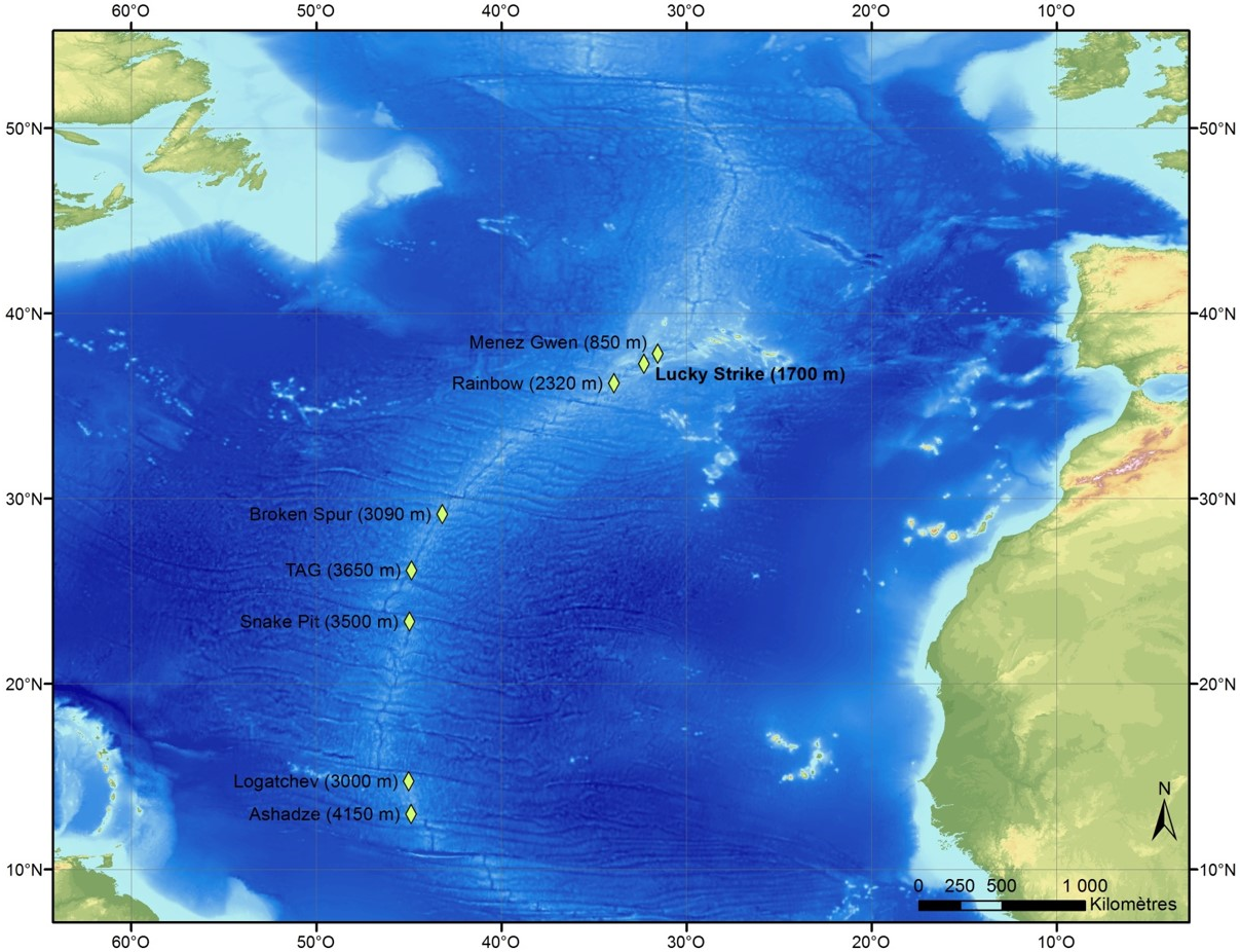
The EMSO-Azores deep-sea observatory on the Mid-Atlantic Ridge supports the long-term monitoring of the Lucky Strike hydrothermal vent field (Figure 2) since 2010. During the annual maintenance cruises (Cannat and Sarradin, 2010), a ROV operated by the French National Institute for Ocean Science (Ifremer) has been used to study the evolution of the hydrothermal circulation and the associated fauna communities over several years (Matabos et al., 2022). Within this field, the hydrothermal vent edifice Eiffel Tower, located at 1700 m beneath the surface, has been extensively studied since its discovery in 1992 (Langmuir et al., 1993). Four dives, in 2015, 2016, 2018 and 2020, were dedicated to the 3D reconstruction of the structure enabling quantitative monitoring of vent community distribution and dynamics (Girard et al., 2020).
| Year | Resolution | Frame rate |
|---|---|---|
| 2015 | 1920x1080 px | 25 fps |
| 2016 | 1920x1080 px | 25 fps |
| 2018 | 1920x1080 px | 25 fps |
| 2020 | 3840x2160 px | 30 fps |
| Model | Nb. of images | Nb. of 3D points | Mean track length | Mean obs. per image | Mean reproj. error |
|---|---|---|---|---|---|
| 2015 | 4,914 | 525,522 | 8.48 | 906.4 | 1.35 px |
| 2016 | 3,699 | 520,320 | 5.85 | 823.5 | 1.32 px |
| 2018 | 5,493 | 618,421 | 7.09 | 798.1 | 1.31 px |
| 2020 | 3,976 | 464,331 | 8.35 | 975.5 | 1.33 px |
| Global | 18,082 | 1,971,726 | 8.24 | 898.7 | 1.39 px |
During the different dives, synchronized videos and navigation data were acquired using the ROV sensors. Videos were captured using two different cameras, whose characteristics are presented in Table 1. Images were acquired through a specifically designed dome port with corrective lenses to account for underwater refraction. As these lenses largely compensate the distortion induced by the air-glass-water mediums, a second order radial distortion model with k1 and k2 distortion coefficient was used to calibrate the cameras underwater. The ROV incorporated an artificial lighting system consisting of 12 LED panels delivering 20,000 lumens each. It also embedded an Ultra-Short Baseline acoustic positioning system (USBL), an Inertial Navigation System (INS), a Doppler Velocity Log (DVL) and a depth sensor that were fused similarly to Guerrero-Font et al. (2016) to compute the navigation data which provide an estimate of the position of the vehicle. This position is composed of the latitude, longitude and altitude of the ROV as well as its yaw, pitch and roll angles. However, navigation data are only consistent within each visit due to the uncertainty of the USBL, which can exhibit offsets of several meters between the frames of the different visits.
4 Camera poses and scene geometry
This visual localization dataset offers images and their 6DOF poses expressed in a common frame of reference. COLMAP SfM (Schönberger and Frahm, 2016) was used to obtain camera poses and intrinsic parameters, as well as 3D scene geometry.
From the videos captured each year, one image was extracted every 3 seconds to create the input data of the dataset. Some images were polluted on their border with small navigation overlays that were removed using an inpainting technique (Telea, 2004). In addition, images were inspected manually to discard irrelevant ones, e.g., images only capturing the water column.
Several issues were encountered when attempting to use COLMAP directly on images from all years. Firstly, to create image pairs, COLMAP relies on image retrieval methods like vocabulary tree (Schönberger et al., 2016) or NetVLAD (Arandjelovic et al., 2016). While these methods successfully match images of the same year, they show poor performance at pairing images across different years. Secondly, to perform feature matching between image pairs, COLMAP uses SIFT descriptors. However, as shown on Figure 3, hand-crafted descriptors fail to produce satisfactory matches between images of different years.
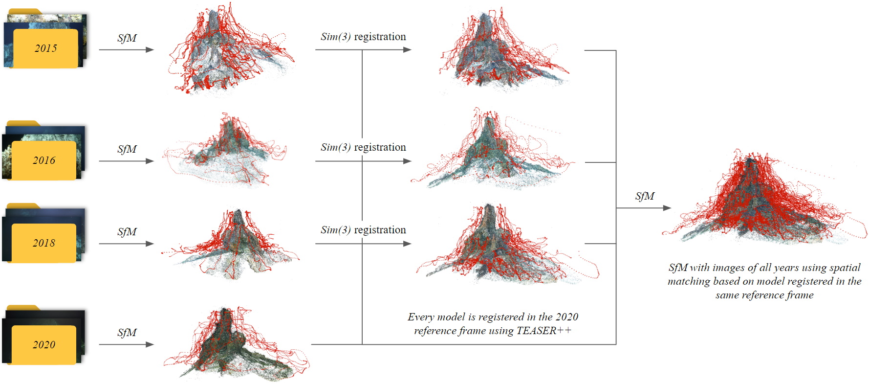
To overcome these issues, we adopted the SfM pipeline described on Figure 4111The code used to compute the different steps of the presented SfM pipeline is available at github.com/clementinboittiaux/sfm-pipeline.. We first built a model for each year independently. For each individual model, image retrieval was performed using navigation data. However, navigation data are missing for 3,178 images of the 2015 dive. In this case, image retrieval was achieved using NetVLAD (Arandjelovic et al., 2016). Within the same visit, NetVLAD proved to be efficient to retrieve similar images. Instead of hand-crafted descriptors, we used SuperPoint (DeTone et al., 2018) and SuperGlue (Sarlin et al., 2020) for feature matching. We then registered the resulting 3D point clouds of each individual model to the 2020 point cloud using TEASER++ (Yang et al., 2021) and refined the result with ICP (Zhou et al., 2018). This way, we obtained a coarse estimation of the camera intrinsics and poses of each year in the same reference frame. We then paired cross-year images using these poses and matched these images with SuperPoint and SuperGlue. Finally, we used COLMAP to obtain a global model embedding all images.
The scale of each model was retrieved by aligning camera poses in with available navigation data using Umeyama’s algorithm (Umeyama, 1991). For the global model that includes all observations, the alignment was performed using only 2020 navigation data. At this point, we have the 6DOF pose of each viewpoint as well as a 3D point cloud of the full vent in the same reference frame at real scale for every year.
| Observation year | 2015 | 2016 | 2018 | 2020 |
|---|---|---|---|---|
| 2015 | 65.9% | 10.7% | 15.2% | 8.12% |
| 2016 | 20.3% | 50.9% | 16.2% | 12.6% |
| 2018 | 16.1% | 9.05% | 63.1% | 11.8% |
| 2020 | 9.79% | 8.00% | 13.5% | 68.8% |
Table 2 reports statistics about the reconstructions obtained with COLMAP as a way to illustrate the certainty level of the proposed ground truth. Table 3 reports the percentage of 3D points matched between each year in the resulting SfM. While the majority of 3D points observations are contained within the same year, a significant proportion of them were matched across different years. This ensures that the scene geometry and camera poses are consistent between the different visits.
5 Dataset format
The Eiffel Tower dataset is composed of images of the dives and a global COLMAP model embedding all visits. For reproducibility purposes, we also provide individual COLMAP models for each visit and interpolated navigation data for each image when available. The dataset architecture is detailed in Figure 5.
Each image is named after the date at which it was acquired in the format YYYYmmddTHHMMSS.fffZ, where YYYY is the four digit year, mm is the month, dd is the day, HH is the hour in the 24 hours format, MM are the minutes, SS the seconds and fff the milliseconds.
A COLMAP model embeds scene geometry, camera intrinsics and poses. It is composed of 3 files: cameras.txt contains the camera intrinsics; images.txt provides camera poses as well as lists of 2D keypoints associated to their 3D observations for each image; points3D.txt consists of the positions and colors of the 3D points. The specificities of COLMAP output format can be found in the documentation222colmap.github.io/format.html. Moreover, COLMAP provides scripts to easily read models in C++, Python and MATLAB333github.com/colmap/colmap/blob/dev/scripts.
Navigation data are provided in the following text format:
image001.png
lat1
lon1
alt1
image002.png
lat2
lon2
alt2
…
where lat, lon and alt are the latitude, longitude and altitude of the vehicle.
.1 EiffelTower. .2 global. .3 sfm. .4 cameras.txt. .4 images.txt. .4 points3D.txt. .2 2015. .3 images. .3 sfm. .3 navigation.txt. .2 2016. .2 2018. .2 2020.
6 Characterizing changes across years
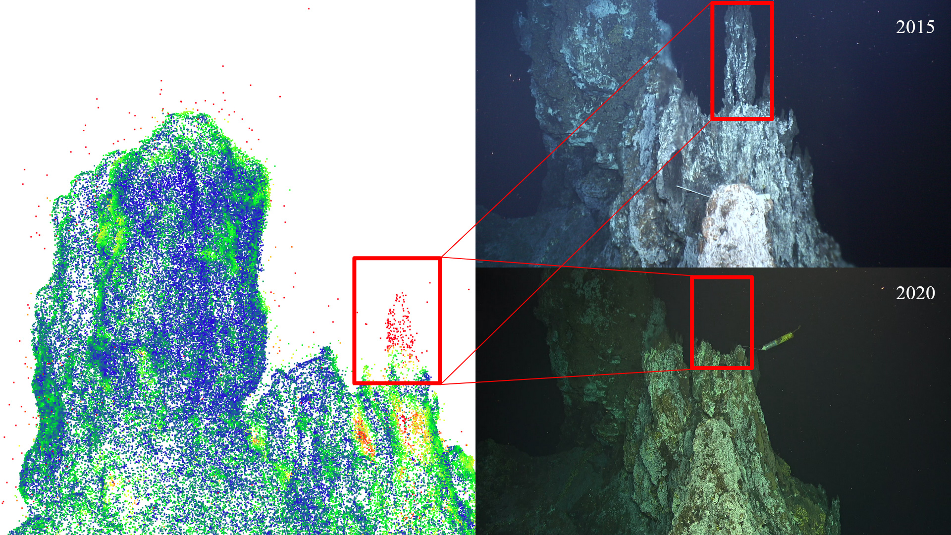
This dataset contains numerous appearance changes across visits that present important challenges for the visual-based localization task. These alterations are of different nature, i.e., topographic, environmental or modifications in the ROV’s equipment. A number of changes observed and measured over the period reflect a modification of the edifice’s local geomorphology over the years (Van Audenhaege et al., 2023). Chimney collapse, outcrop/boulder detachment or slide resulted in a loss of material, while vent active areas grew through mineral accretion creating new outcrops, flanges and spires. Material build-up was twice as important as the loss, suggesting that the volume of the edifice is increasing over time. While these changes can be locally drastic and affect the registration of 3D models over the years, they represent only 5% of the total surface and are localized in areas of active venting. Local changes in hydrothermal activity also result in distinct mineralization processes, hence deposits, the color of which will vary depending on the temperature and chemical composition of the fluid. Figure 6 reveals a modification in the topography of the scene. A chimney visible in 2015 is missing in 2020, and a temperature sensor, absent in 2015, was deployed in the vicinity in 2020.
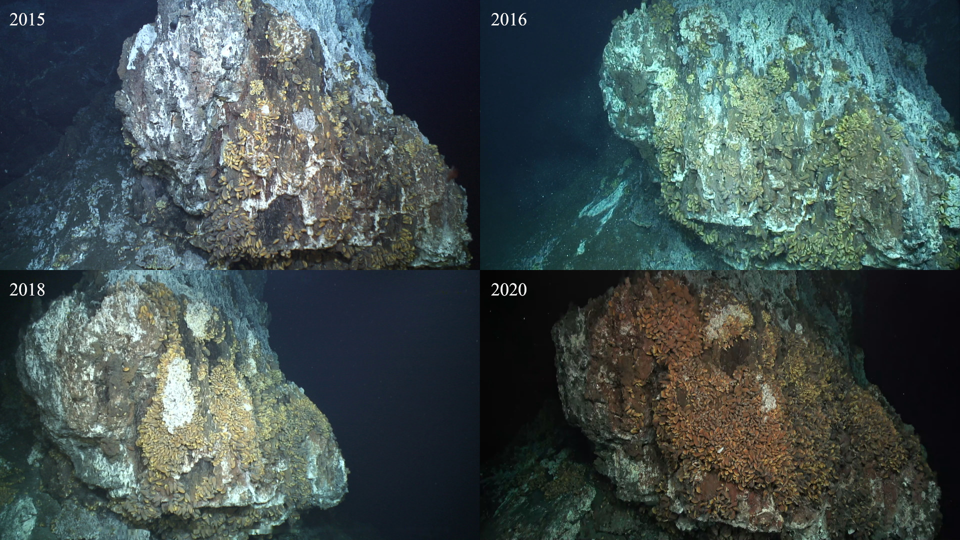
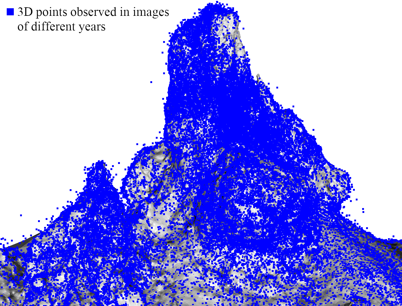
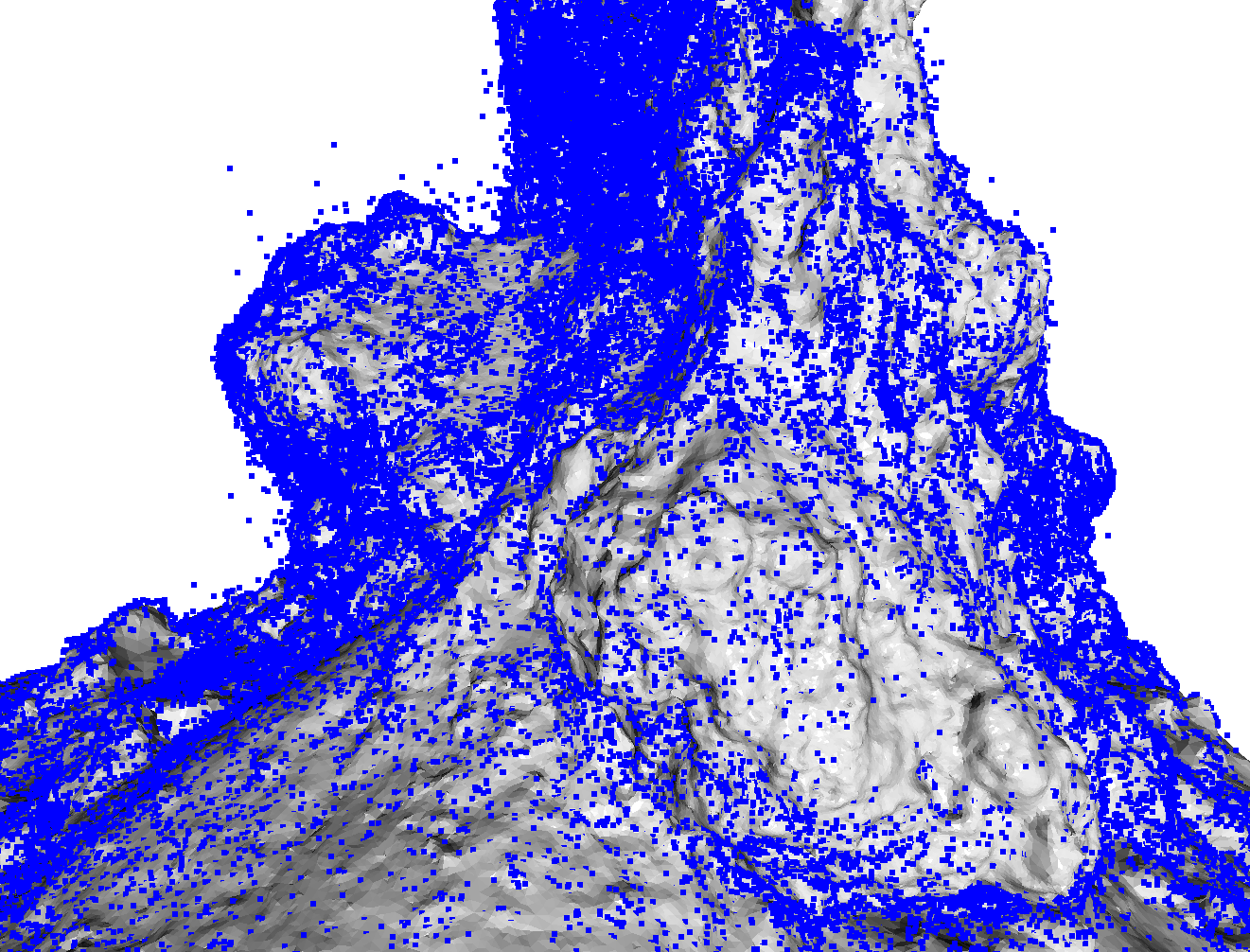
Biological changes were more important and mainly localized in areas of topographic changes. They result from mussel populations that grow and migrate to colonize newly created habitats (143.97 m2 from 2015 to 2020) (Van Audenhaege et al., 2022). Moreover, mussels are dynamically reoriented on a daily basis. Furthermore, the period from 2015 to 2020 showed an overall disappearance of white microbial mats over the whole edifice (-72.85 m2). Although these changes do not affect the general topography of the structure, they strongly modify the color and texture of the model. Figure 7 illustrates how the mussels’ population evolution over the years can alter both the topography of the scene and the colors of the vent. Also, because of these organic modifications, there are no real matching 3D points between different years on most of the chimney. This makes it difficult to match specific 2D points. Figure 8 shows how these biological changes affect the global 3D reconstruction of the edifice. While the vent is overall well matched across different years, some specific areas like the south-east façade suffer from this source of variability and the model mostly relies on matches between images of the same year.
| Method | Median errors | 1 cm, 1° | 2 cm, 2° | 3 cm, 3° | 5 cm, 5° | 25 cm, 2° | 50 cm, 5° | 500 cm, 10° |
|---|---|---|---|---|---|---|---|---|
| PoseNet | 1.98 m, 10.73° | 0.00% | 0.00% | 0.00% | 0.02% | 0.24% | 3.58% | 45.75% |
| Homoscedastic | 1.32 m, 6.27° | 0.00% | 0.00% | 0.00% | 0.00% | 0.79% | 10.20% | 62.03% |
| Homography | 1.23 m, 8.30° | 0.00% | 0.00% | 0.00% | 0.02% | 0.53% | 8.47% | 57.83% |
| hLoc | 0.09 m, 1.11° | 15.04% | 28.37% | 36.04% | 43.49% | 53.87% | 57.94% | 60.07% |
| PixLoc | 6.55 m, 41.00° | 0.41% | 1.75% | 3.50% | 6.49% | 13.76% | 15.16% | 18.46% |
| hLoc+PixLoc | 0.08 m, 1.10° | 13.41% | 28.18% | 35.80% | 44.08% | 53.95% | 57.94% | 60.07% |
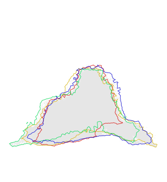
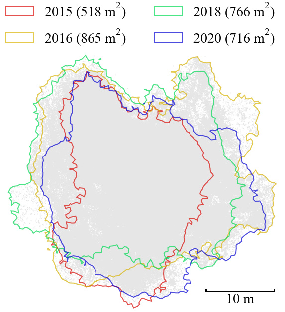
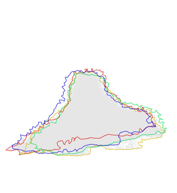
Figure 9 displays the area covered by the ROV each year. We notice that the vehicle covered uneven regions over the different years. The 2015 dive covered the least amount of ground compared to all other years.
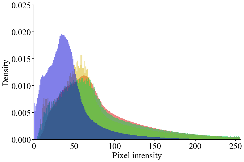
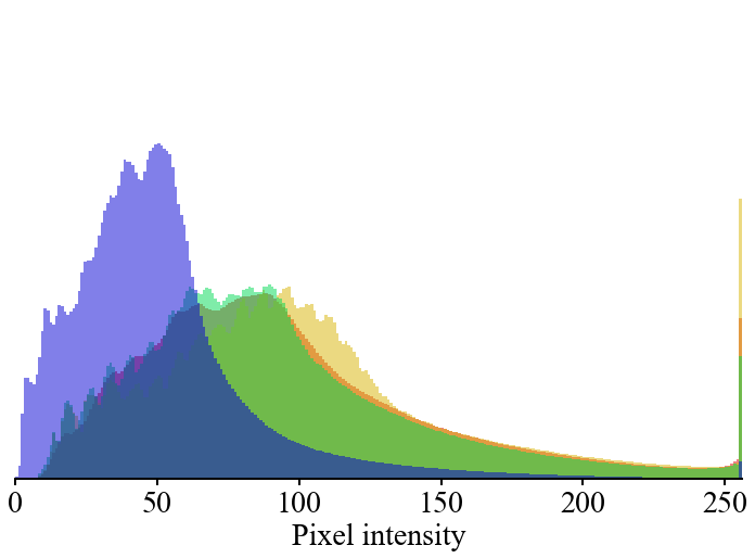
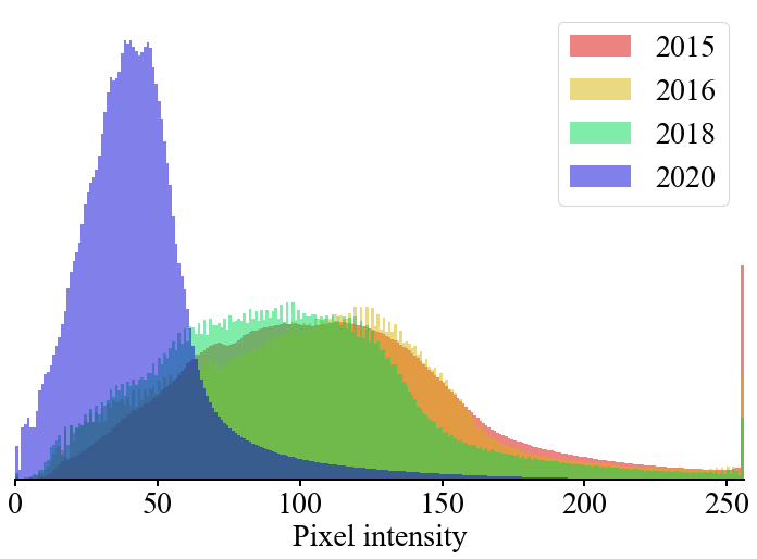
Figure 10 compares the histograms of pixel intensities in all images of each year. First, we observe that the red channel has an overall lower pixel intensity when compared to the green and blue channels. This is easily explained by the attenuation difference of the wavelengths due to the underwater environment (Akkaynak and Treibitz, 2019; Berman et al., 2021). We also notice a shift in pixel intensity for the 2020 dive, which is likely due to the change of camera.
7 Visual localization benchmark
Train and test sets were separated based on the area covered by the ROV each year. As seen on Figure 9, the total area covered in 2016, 2018 and 2020 contains almost all the area covered in 2015. As a result, we chose 2016, 2018 and 2020 as the train set and 2015 as the test set.
Using the aforementioned train/test split, we benchmarked the Eiffel Tower dataset on renowned visual localization methods: PoseNet with different losses (Kendall et al., 2015; Kendall and Cipolla, 2017; Boittiaux et al., 2022), hLoc (Sarlin et al., 2019) and PixLoc (Sarlin et al., 2021). PoseNet trains a different neural network for each scene, while hLoc and PixLoc rely on deep-learning based features trained on terrestrial datasets. We detail below the parameters used for each of the methods.
PoseNet
444An implementation of PoseNet with all three pose regression losses is available at github.com/clementinboittiaux/homography-loss-function.: The network as described in (Kendall et al., 2015) is re-implemented, except for replacing the GoogLeNet backbone with a more modern MobileNetV2 (Sandler et al., 2018). For PoseNet loss, we used as suggested in (Kendall et al., 2015) for the outdoor Cambridge dataset. We initialized the Homoscedastic loss as suggested in (Kendall and Cipolla, 2017), i.e., and . For the Homography loss, we selected local and as the and percentile, as presented in (Boittiaux et al., 2022).
hLoc
: We use the pipeline presented in (Sarlin et al., 2019), i.e., NetVLAD for image retrieval and SuperPoint alongside SuperGlue pre-trained on outdoor scenes for local matching.
PixLoc
: We used weights of the network pre-trained on the MegaDepth dataset (Li and Snavely, 2018).
hLoc+PixLoc
: The pose of the camera is first retrieved using hLoc and then refined with PixLoc. This pipeline is presented by Sarlin et al. (2021).
Results on the dataset for all aforementioned methods are reported in Table 4 and can be used as a baseline for the comparison of other long-term visual localization methods. Unlike hLoc and Pixloc, PoseNet based methods are end-to-end networks. Consistent with the results presented by Sattler et al. (2019), end-to-end networks obtain the least accurate pose estimates. Moreover, since the ground truth was constructed using SfM, methods that replicate this mode of operation, e.g. hLoc, have an advantage because they optimize the same metric (Brachmann et al., 2021).
hLoc and PixLoc are based on networks trained on terrestrial data, and we can expect better results by training these networks on aquatic data. However, this remains a challenge because the amount of data needed exceeds what is readily available for the underwater environment. For example, NetVLAD is trained on Google Street View Time Machine. Another approach would be to minimize the changes due to physical phenomena induced by the underwater environment to get closer to terrestrial images, using for example algorithms like Sea-thru (Akkaynak and Treibitz, 2019) or SUCRe (Boittiaux et al., 2023).
8 Conclusion
This paper presented a novel dataset to evaluate visual localization methods in deep-sea environments. Unlike pre-existing datasets, Eiffel Tower presents long-term changes in underwater scenarios, e.g., topography, population and species distribution, backscatter and color attenuation. We analyzed these changes and evaluated several localization pipelines on the proposed dataset. The obtained results can be used as a baseline for future work on underwater visual localization systems. Besides its use for visual localization, this dataset can also be employed to detect changes in the scene’s geometry in deep-sea environments. More generally, it may also be useful to study the effects of water on various computer vision algorithms.
All data acquisitions were conducted by Ifremer. The authors would like to thank the crews of the research vessels, Pourquoi Pas? and L’Atalante, the pilots of the ROV Victor6000, as well as all the personnel who helped in acquiring these data. MM and LVA were supported by the European Union’s Horizon 2020 research and innovation project iAtlantic under Grant Agreement No. 818123.
References
- Akkaynak and Treibitz (2019) Akkaynak D and Treibitz T (2019) Sea-Thru: A method for removing water from underwater images. In: Proceedings of the IEEE Conference on Computer Vision and Pattern Recognition (CVPR). pp. 1682–1691.
- Arandjelovic et al. (2016) Arandjelovic R, Gronat P, Torii A, Pajdla T and Sivic J (2016) NetVLAD: CNN architecture for weakly supervised place recognition. In: Proceedings of the IEEE Conference on Computer Vision and Pattern Recognition (CVPR). Las Vegas, United States, pp. 5297–5307.
- Berman et al. (2021) Berman D, Levy D, Avidan S and Treibitz T (2021) Underwater single image color restoration using haze-lines and a new quantitative dataset. Proceedings of the IEEE Transactions on Pattern Analysis and Machine Intelligence 43(8): 2822–2837.
- Boittiaux et al. (2023) Boittiaux C, Marxer R, Dune C, Arnaubec A, Ferrera M and Hugel V (2023) SUCRe: Leveraging scene structure for underwater color restoration. Under review.
- Boittiaux et al. (2022) Boittiaux C, Marxer R, Dune C, Arnaubec A and Hugel V (2022) Homography-based loss function for camera pose regression. IEEE Robotics and Automation Letters 7(3): 6242–6249.
- Brachmann et al. (2021) Brachmann E, Humenberger M, Rother C and Sattler T (2021) On the limits of pseudo ground truth in visual camera re-localisation. In: Proceedings of the IEEE International Conference on Computer Vision (ICCV). pp. 6198–6208.
- Burnett et al. (2023) Burnett K, Yoon DJ, Wu Y, Li AZ, Zhang H, Lu S, Qian J, Tseng WK, Lambert A, Leung KY, Schoellig AP and Barfoot TD (2023) Boreas: A multi-season autonomous driving dataset. The International Journal of Robotics Research 42(1-2): 33–42.
- Campos et al. (2015) Campos R, Garcia R, Alliez P and Yvinec M (2015) A surface reconstruction method for in-detail underwater 3D optical mapping. The International Journal of Robotics Research 34(1): 64–89.
- Cannat and Sarradin (2010) Cannat M and Sarradin PM (2010) MOMARSAT : Monitoring the Mid Atlantic Ridge. 10.18142/130.
- Cernea (2020) Cernea D (2020) OpenMVS: Multi-view stereo reconstruction library.
- DeTone et al. (2018) DeTone D, Malisiewicz T and Rabinovich A (2018) SuperPoint: Self-supervised interest point detection and description. In: Proceedings of the IEEE Conference on Computer Vision and Pattern Recognition (CVPR) Workshops. pp. 337–33712.
- Ferrera et al. (2019) Ferrera M, Creuze V, Moras J and Trouvé-Peloux P (2019) AQUALOC: An underwater dataset for visual–inertial–pressure localization. The International Journal of Robotics Research 38(14): 1549–1559.
- Girard et al. (2020) Girard F, Sarrazin J, Arnaubec A, Cannat M, Sarradin PM, Wheeler B and Matabos M (2020) Currents and topography drive assemblage distribution on an active hydrothermal edifice. Progress in Oceanography 187: 102397.
- Griffith et al. (2017) Griffith S, Chahine G and Pradalier C (2017) Symphony lake dataset. The International Journal of Robotics Research 36(11): 1151–1158.
- Guerrero-Font et al. (2016) Guerrero-Font E, Massot-Campos M, Negre PL, Bonin-Font F and Codina GO (2016) An USBL-aided multisensor navigation system for field AUVs. In: IEEE International Conference on Multisensor Fusion and Integration for Intelligent Systems (MFI). pp. 430–435.
- Kendall and Cipolla (2017) Kendall A and Cipolla R (2017) Geometric loss functions for camera pose regression with deep learning. In: Proceedings of the IEEE Conference on Computer Vision and Pattern Recognition (CVPR). pp. 5974–5983.
- Kendall et al. (2015) Kendall A, Grimes M and Cipolla R (2015) PoseNet: A convolutional network for real-time 6-dof camera relocalization. In: Proceedings of the IEEE International Conference on Computer Vision (ICCV). pp. 2938–2946.
- Langmuir et al. (1993) Langmuir C, Charlou JL, Colodner D, Costa I, Desbruyeres D, Desonie D, Emerson T, Fornari D, Fouquet Y, Humphris S, Fiala-Medioni A, Saldanha L, Sours-Page R, Thatcher M, Tivey M, Dover C, Damm K, Wiese K and Wilson C (1993) Lucky Strike - A newly discovered hydrothermal site on the Azores platform. Ridge Events 4(2): 3–5.
- Li et al. (2019) Li C, Guo C, Ren W, Cong R, Hou J, Kwong S and Tao D (2019) An underwater image enhancement benchmark dataset and beyond. IEEE Transactions on Image Processing 29: 4376–4389.
- Li and Snavely (2018) Li Z and Snavely N (2018) MegaDepth: Learning single-view depth prediction from internet photos. In: Proceedings of the IEEE Conference on Computer Vision and Pattern Recognition (CVPR). pp. 2041–2050.
- Mallios et al. (2017) Mallios A, Vidal E, Campos R and Carreras M (2017) Underwater caves sonar data set. The International Journal of Robotics Research 36(12): 1247–1251.
- Matabos et al. (2022) Matabos M, Barreyre T, Juniper SK, Cannat M, Kelley D, Alfaro-Lucas JM, Chavagnac V, Colaço A, Escartin J, Escobar E, Fornari D, Hasenclever J, Huber JA, Laës-Huon A, Lantéri N, Levin LA, Mihaly S, Mittelstaedt E, Pradillon F, Sarradin PM, Sarrazin J, Tomasi B, Venkatesan R and Vic C (2022) Integrating Multidisciplinary Observations in Vent Environments (IMOVE): Decadal Progress in Deep-Sea Observatories at Hydrothermal Vents. Frontiers in Marine Science 9.
- Nielsen et al. (2019) Nielsen MC, Leonhardsen MH and Schjølberg I (2019) Evaluation of PoseNet for 6-dof underwater pose estimation. In: OCEANS 2019 MTS/IEEE. pp. 1–6.
- Sandler et al. (2018) Sandler M, Howard A, Zhu M, Zhmoginov A and Chen LC (2018) MobileNetV2: Inverted residuals and linear bottlenecks. In: Proceedings of the IEEE Conference on Computer Vision and Pattern Recognition (CVPR). pp. 4510–4520.
- Sarlin et al. (2019) Sarlin PE, Cadena C, Siegwart R and Dymczyk M (2019) From coarse to fine: Robust hierarchical localization at large scale. In: Proceedings of the IEEE Conference on Computer Vision and Pattern Recognition (CVPR). pp. 12716–12725.
- Sarlin et al. (2020) Sarlin PE, DeTone D, Malisiewicz T and Rabinovich A (2020) SuperGlue: Learning feature matching with graph neural networks. In: Proceedings of the IEEE Conference on Computer Vision and Pattern Recognition (CVPR). pp. 4938–4947.
- Sarlin et al. (2021) Sarlin PE, Unagar A, Larsson M, Germain H, Toft C, Larsson V, Pollefeys M, Lepetit V, Hammarstrand L, Kahl F et al. (2021) Back to the feature: Learning robust camera localization from pixels to pose. In: Proceedings of the IEEE Conference on Computer Vision and Pattern Recognition (CVPR). pp. 3247–3257.
- Sattler et al. (2018) Sattler T, Maddern W, Toft C, Torii A, Hammarstrand L, Stenborg E, Safari D, Okutomi M, Pollefeys M, Sivic J et al. (2018) Benchmarking 6DOF outdoor visual localization in changing conditions. In: Proceedings of the IEEE Conference on Computer Vision and Pattern Recognition (CVPR). pp. 8601–8610.
- Sattler et al. (2019) Sattler T, Zhou Q, Pollefeys M and Leal-Taixe L (2019) Understanding the limitations of CNN-based absolute camera pose regression. In: Proceedings of the IEEE Conference on Computer Vision and Pattern Recognition (CVPR). pp. 3302–3312.
- Schönberger and Frahm (2016) Schönberger JL and Frahm JM (2016) Structure-from-Motion revisited. In: Proceedings of the IEEE Conference on Computer Vision and Pattern Recognition (CVPR). pp. 4104–4113.
- Schönberger et al. (2016) Schönberger JL, Price T, Sattler T, Frahm JM and Pollefeys M (2016) A vote-and-verify strategy for fast spatial verification in image retrieval. In: Asian Conference on Computer Vision. Springer, pp. 321–337.
- Shotton et al. (2013) Shotton J, Glocker B, Zach C, Izadi S, Criminisi A and Fitzgibbon A (2013) Scene coordinate regression forests for camera relocalization in RGB-D images. In: Proceedings of the IEEE Conference on Computer Vision and Pattern Recognition (CVPR). pp. 2930–2937.
- Telea (2004) Telea A (2004) An image inpainting technique based on the fast marching method. Journal of Graphics Tools 9(1): 23–34.
- Umeyama (1991) Umeyama S (1991) Least-squares estimation of transformation parameters between two point patterns. Proceedings of the IEEE Transactions on Pattern Analysis and Machine Intelligence 13(4): 376–380.
- Valentin et al. (2016) Valentin J, Dai A, Niessner M, Kohli P, Torr P, Izadi S and Keskin C (2016) Learning to navigate the energy landscape. In: 2016 Fourth International Conference on 3D Vision (3DV). pp. 323–332.
- Van Audenhaege et al. (2022) Van Audenhaege L, Matabos M, Brind’Amour A, Drugmand J, Laës-Huon A, Sarradin PM and Sarrazin J (2022) Long-term monitoring reveals unprecedented stability of a vent mussel assemblage on the Mid-Atlantic Ridge. Progress in Oceanography 204: 102791.
- Van Audenhaege et al. (2023) Van Audenhaege L, Sarrazin J, Legendre P, Perrois G, Cannat M and Matabos M (2023) Monitoring ecological dynamics on complex hydrothermal structures: a novel photogrammetry approach reveals fine scales of faunal assemblage variability. Under review.
- Yang et al. (2021) Yang H, Shi J and Carlone L (2021) TEASER: Fast and certifiable point cloud registration. IEEE Transactions on Robotics 37(2): 314–333.
- Zhou et al. (2018) Zhou QY, Park J and Koltun V (2018) Open3D: A modern library for 3D data processing. arXiv:1801.09847 .
