Causal Discovery with Unobserved Variables:
A Proxy Variable Approach

Abstract

Discovering causal relations from observational data is important. The existence of unobserved variables, such as latent confounders or mediators, can mislead the causal identification. To address this issue, proximal causal discovery methods proposed to adjust for the bias with the proxy of the unobserved variable. However, these methods presumed the data is discrete, which limits their real-world application. In this paper, we propose a proximal causal discovery method that can well handle the continuous variables. Our observation is that discretizing continuous variables can can lead to serious errors and comprise the power of the proxy. Therefore, to use proxy variables in the continuous case, the critical point is to control the discretization error. To this end, we identify mild regularity conditions on the conditional distributions, enabling us to control the discretization error to an infinitesimal level, as long as the proxy is discretized with sufficiently fine, finite bins. Based on this, we design a proxy-based hypothesis test for identifying causal relationships when unobserved variables are present. Our test is consistent, meaning it has ideal power when large samples are available. We demonstrate the effectiveness of our method using synthetic and real-world data.

1 Introduction

Causal discovery has received increasing attention due to its wide application in machine learning, medicine, and psychology. While the golden standard for causal discovery remains randomized experimentation (RCT), it can be too expensive, unethical, or even impossible to conduct in the real world. For this reason, identifying causal relations from pure observation data is desirable.

A well-known issue of inferring causation from observation is the existence of unobserved variables, such as latent confounders [1] and mediators [2]. These variables describe intrinsic characteristics that are widely present but difficult to quantify (e.g. health status, gene), and hence induce strong bias for the causal identification.

To address this problem, recent studies have proposed using a proxy variable to correct for the bias caused by the unobserved variable. Here, the proxy variable can be a noisy measurement or an observed child of the unobserved variable, from which useful information about the latent bias can be inferred. For example, [3] developed a matrix adjustment method based on prior knowledge of the proxy generation mechanism; [4] showed that the generation mechanism could be automatically identified, thus avoiding the need for external information. Based on this, [5, 6] proposed a proxy-based hypothesis test to distinguish causation from latent confounding, and [7] treated the proxy as a negative control outcome and employed control outcome calibration [8] for identification.

Despite the progress that has been made, these works rely heavily on an assumption that all variables in the system are discrete, in order to conduct matrix operations and valid independence tests. However, this critical assumption does not apply in many real-life scenarios where variables, such as the dosage of medicines and readings of vital signs, are inherently continuous. For such cases, applying these discrete methods directly can result in severe misidentification [9, 10]. This problem, together with the practical usage of the proxy variable, is illustrated by the following example.

Example 1.1.

Prescription opioids (e.g., morphine, oxycodone) have been traditionally used as pain relievers in patients with severe disease [11]. Despite their wide usage, critics often question their safety, citing a higher mortality rate associated with opioid use [12]. Indeed, this association can be a confounding bias induced by the hidden health status, according to recent RCTs [13, 14], in the sense that patients with poorer health often require more opioids to ease the pain, and meanwhile are more likely to die. To remove the bias, we can use the patient’s vital sign, e.g., blood pressure, as the proxy variable. However, as shown in Fig. 1 (b), naively applying the discrete method leaves the bias remaining. This is because the discretization error can break key independence in the proximal model (Fig. 1 (c)) and therefore compromise the power of the proxy variable.

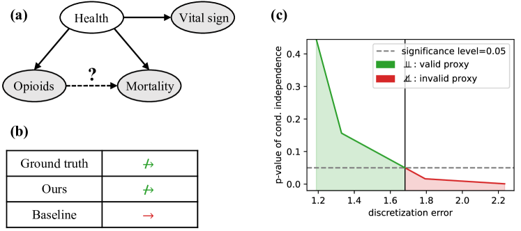
Figure 1: Illustration of Exam. 1.1. (a) The underlying causal graph with observed variables marked gray. (b) Identification results with our method and naive baseline [5]. (c) Large discretization errors break key conditional independence that the proxy variable relies on.

In this paper, we propose a hypothesis-test-based method that can use a single continuous proxy to achieve causal identification. To this end, we first propose to identify the source of the discretization error. We further show that this error can be effectively controlled if the conditional distribution of the proxy given the unobserved variable changes smoothly with the latter. Pleasingly, this smoothness condition we identify is mild and requires nothing but continuity and differentiability of the structural equation. Based on this analysis, we propose a hypothesis test to identify the causal relation with the proxy variable. We show that our test is consistent, given large samples and sufficiently fine, finite partitions of the continuous variables.

Back to the opioids example, Fig. 1 (b) shows that our test can identify the causal relation that well aligns with the RCT findings, while compared baselines fail to do so.

Our contributions are summarized as follows:

1. We identify mild conditions under which the discretization error can be controlled.

2. We propose a proximal causal discovery method that can well handle continuous variables.

3. We achieve more accurate causal identification than others on synthetic and real data.

2 Related works

Proximal causal discovery. The use of proxy to adjust for latent bias can be traced back to the seminal work of [3], who developed a matrix adjustment method that required external knowledge about the proxy generation mechanism. To ease this requirement, [4] showed that for surrogate-rich setting, i.e., cases with multiple proxies, one could identify the error mechanism and thus the causal relation without external information. Following this work, the surrogate-rich setting has been extensively studied in [15, 16, 17, 18, 19]. On the other side, identification with a single proxy, though of higher practical value, has been hard to come by. For example, the method in [7] could not achieve complete identification. [5, 6], the works most similar to ours, only applied to discrete variables satisfying particular level constraints. In contrast, we propose a general framework that can achieve complete identification with a single continuous proxy.

Conditional independence (CI) test with discretization. Causal discovery is closely related to the test of CI, since the correlation between two variables is believed to be causation only if it does not disappear conditioning on a third variable [20]. Since testing CI is much easier in the discrete case, many attempts have been made to test continuous CI via discretization [10, 21]. Nonetheless, general theoretical guarantees for such discretization were not carefully studied until the recent work of [22]. In [22], the authors imposed smoothness assumptions on the conditional distributions, so that if one binned the conditioning variable with sufficient refined partitions, the problem of testing continuous CI could be converted (with tractable cost) to that of testing discrete CI in each partition. Such an idea is further exploited under weaker assumptions in [23]. However, these methods required the conditioning variable to be observable. As a contrast, we consider cases where the conditioning variable is unobservable and hence can not be directly discretized.

3 Preliminary

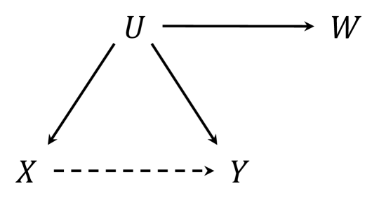
(a)

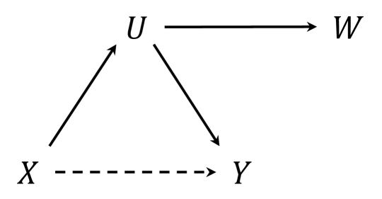
(b)

Figure 2: Proximal causal discovery. $X\dashrightarrow Y$ is the causal edge of interest. $U$ is the unobserved variable, which can be a (a) confounder or (b) mediator. $W$ is the proxy variable of $U$.

Problem setup. We consider the problem of identifying the causal relationship between a pair of variables, $X$ and $Y$. The system also includes an unobserved variable $U$, which can be either a sufficient confounder or mediator between $X$ and $Y$. For this case, causal identification is generally not feasible due to the confounding [1] or mediation bias [2]. To adjust for the bias, we assume the availability of a proxy variable $W$. In practice, the proxy variable can be a noisy measurement or an observed child of the unobserved variable $U$. We illustrate the relations between $X,Y,U,W$ with models (2)-(2) in Fig. 2.

Notations. We use $\mathcal{P}_{X},\mathcal{P}_{X,Y},\mathcal{P}_{X|Y}$ to (resp.) denote the marginal, joint, and conditional distributions. We use $pr(X=x)$ ($pr(x)$ for short) and $pr(X\in A)$ to (resp.) denote the probabilities of “$X$ takes the value $x$” and “$X$ takes values in the set $A$”. For discrete variables $U,W$ with (resp.) $J,K$ levels, we use $P(W|u):=\left\{pr(w_{1}|u),...,pr(w_{K}|u)\right\}^{T}$ and $P(w|U):=\left\{pr(w|u_{1}),...,pr(w|u_{J})\right\}$ to denote the column and row vectors consist of transition probabilities. The transition matrix from $U$ to $W$ is defined as $P(W|U):=\left\{P(W|u_{1}),...,P(W|u_{J})\right\}$.

Identification in the discrete case. When the system is composed of discrete variables, [5] proposed to identify the causal relation by testing the null causal hypothesis $\mathbb{H}_{0}:X\perp\!\!\!\!\perp Y|U$. The $\mathbb{H}_{0}$ means there is no (direct) causal influence between $X$ and $Y$, and a rejection of $\mathbb{H}_{0}$ is, therefore, evidence in favor of causation.

The null hypothesis holds if and only if $\mathcal{P}_{Y|U,X}=\mathcal{P}_{Y|U}$. Hence, to test $\mathbb{H}_{0}$, [5] proposed to measure the divergence $pr(y|u,x)-pr(y|u)$ based on the proxy variable $W$. Specifically, suppose that $X,U,W$ are discrete variables with (resp.) $I,J,K$ levels such that $I>J=K$. Models (2)-(2) indicate $W\perp\!\!\!\!\perp X|U$ and hence:

$$P(W|x)=P(W|U)P(U|x),\,\,\,pr(y|x)=P(y|U,x)P(U|x).$$

Suppose the matrix $P(W|U)$ is invertible, the two equations together imply:

$$pr(y|x)=P(y|U)P(W|U)^{-1}P(W|x)+\{P(y|U,x)-P(y|U)\}P(W|U)^{-1}P(W|x).$$ (1)

For fixed $y$, as $x$ varies, (1) reveals two separate sources of variability in $pr(y|x)$: $P(W|x)$ and $P(y|U,x)$. If $\mathbb{H}_{0}$ holds, the divergence term $P(y|U,x)-P(y|U)$ will be zero, and $P(W|x)$ will be the only source of variability. Based on this, [5] proposed to test $\mathbb{H}_{0}$ by checking whether $P(W|x)$ explains away the variability of $pr(y|x)$. In detail, denote $q_{y}:=P(y|X)$ and $Q:=P(W|X)$. Suppose that there are estimators $(\hat{q}_{y},\hat{Q})$ that satisfy:

$$n^{\frac{1}{2}}(\hat{q}_{y}-q_{y}) \to N(0,\Sigma_{y})\,\,\text{in distribution},$$ (2)

$$\hat{Q}\to Q\,\,\text{and}\,\,\hat{\Sigma}_{y}\to\Sigma_{y}\,\, \text{in probability},\,\,\text{with $\hat{\Sigma}_{y},\Sigma_{y}$ positive-definite}.$$ (3)

If $P(W|x)$ explains away the variability in $pr(y|x)$, there should be a linear relation between $q_{y}$ and $Q$ and the least square residual of regressing $\hat{q}_{y}$ on $\hat{Q}$ should be small.

Formally, denote $I_{n}$ the identity matrix. let $\xi_{y}:=\{I_{n}-\hat{\Sigma}_{y}^{-\frac{1}{2}}\hat{Q}^{T}(\hat{Q}\hat{\Sigma}_{y}^{-1}\hat{Q}^{T})^{-1}\hat{Q}\hat{\Sigma}_{y}^{-\frac{1}{2}}\}\hat{\Sigma}_{y}^{-\frac{1}{2}}\hat{q}_{y}$ be the least square residual of regressing $\hat{\Sigma}_{y}^{-\frac{1}{2}}\hat{q}_{y}$ on $\hat{\Sigma}_{y}^{-\frac{1}{2}}\hat{Q}$. Let $T_{y}:=n\xi_{y}^{T}\xi_{y}$ be the test statistic. When the matrix $Q$ has full row rank, [5] showed that:

Theorem 3.1 ([5], Thm. 2).

If $\mathbb{H}_{0}$ is correct, then $T_{y}\to\chi^{2}_{r}$ in distribution, with $r:=I-K$.

With Thm. 3.1, for a given significance level $\alpha$, one can reject $\mathbb{H}_{0}$ as long as $T_{y}$ exceeds the $(1-\alpha)$-th quantile of $\chi^{2}_{r}$, which guarantees a type-I error no larger than $\alpha$ asymptotically.

However, a major weakness of Thm. 3.1 is that it only applies to discrete variables with strict level constraints ($I>J=K$). In the following section, we will fix this problem and extend Thm. 3.1 to the continuous case.

4 Methodology

In this section, we introduce our method to test the null causal hypothesis with continuous variables. The idea is to discretize the continuous $X,Y,W$ into their discrete copies $\tilde{X},\tilde{Y},\tilde{W}$, and hence covert the problem of testing $X\perp\!\!\!\!\perp Y|U$ to the problem of testing whether $X\perp\!\!\!\!\perp Y|U\in some\,\,bin$. Indeed, there can be a large discrepancy between the two problems due to discretization errors [9].

To overcome the gap, we propose to impose smoothness assumptions on the conditional distribution $\mathcal{P}_{Y|U,X}$, such that one may treat observations from the same bin as if they come from the same distribution, up to some small and controllable errors. These smoothness conditions, as we will show later, are satisfied by a wide range of structural causal models.

The rest of the section is organized as follows. First, in Sec. 4.1, we overview the testing procedure and identify where the discretization errors may occur. Then, in Sec. 4.2, we discuss how to control these errors with smoothness regularities. Finally, in Sec. 4.3, we show that the proper control of the discretization errors leads to an asymptotically valid hypothesis test.

4.1 Identifying sources of the discretization error

In this section, we provide an overview of our testing procedure and identify steps where discretization errors may occur. Here, our strategy is to bin the continuous variables $X,Y,W$ into their discrete copies $\tilde{X},\tilde{Y},\tilde{W}$ and apply the test to the latter ones.

To be specific, for continuous variables $X,U,W$ with bounded supports, let $\{A_{i}\}_{i=1}^{I},\{B_{j}\}_{j=1}^{J},$ $\{C_{k}\}_{k=1}^{K}$ be (resp.) the measurable partitions of $supp(X),supp(U),supp(W)$, and denote the partitioned discrete variables (resp.) as $\tilde{X},\tilde{U},\tilde{W}$. By the law of total probability, we have:

$$pr(W\in C_{k}|x) =\sum\nolimits_{j}pr(W\in C_{k}|U\in B_{j},x)\,\,pr(U\in B_{j}|x),$$

$$pr(y|x) =\sum\nolimits_{j}pr(y|U\in B_{j},x)\,\,pr(U\in B_{j}|x).$$

In the form of transition matrices, these mean:

$${P}(\tilde{W}|x)={P}(\tilde{W}|\tilde{U},x){P}(\tilde{U}|x),\,\,\,pr(y|x)={P}(y|\tilde{U},x){P}(\tilde{U}|x).$$

Now, suppose that

Assumption 4.1.

The matrix ${P}(\tilde{W}|\tilde{U},x)$ is invertible for all $x\in supp(X)$.

Under Asm. 4.1, we can combine the two equations together by inversing the $P(\tilde{W}|\tilde{U},x)$ and have:

$$pr(y|x)={P}(y|\tilde{U},x)\mathbb{P}(\tilde{W}|\tilde{U},x)^{-1}{P}(\tilde{W}|x).$$

Heuristically, we want the following approximations: $P(y|\tilde{U},x)\approx P(y|\tilde{U})$ under $\mathbb{H}_{0}\!:\!X\perp\!\!\!\!\perp Y|U$, and $P(\tilde{W}|\tilde{U},x)\approx P(\tilde{W}|\tilde{U})$ under the proximal models (2)-(2) with $X\perp\!\!\!\!\perp W|U$. If the above approximations are true, we will have:

$$pr(y|x)\approx{P}(y|\tilde{U}){P}(\tilde{W}|\tilde{U})^{-1}{P}(\tilde{W}|x),$$ (4)

which means $pr(y|x)$ varies linearly with $P(\tilde{W}|x)$ under $\mathbb{H}_{0}$. In this regard, the linearity-based test in Thm. 3.1 can be transferred seamlessly to the continuous case.

Indeed, the above analysis relies on two important premises, i.e., $X\perp\!\!\!\!\perp Y|U\Rightarrow P(y|\tilde{U},x)\approx P(y|\tilde{U})$ and $X\perp\!\!\!\!\perp W|U\Rightarrow P(\tilde{W}|\tilde{U},x)\approx P(\tilde{W}|\tilde{U})$. In other words, it requires that the continuous conditional independence (CI) test can be (tractably) converted to the discrete CI test in each bin, and that the proxy variable $W$ retains its power after discretization.

Unfortunately, for the general case, these requirements are not feasible due to discretization errors [9]. Nonetheless, as we show in the next section, there are mild conditions under which the discretization errors can be controlled.

4.2 Controlling the discretization error

In this section, we introduce our strategy to control the discretization errors. Before preceding any technical detail, we first summarize our idea below. Specifically, the objective of interest is to have:

$$\left|pr(y|U\in B_{j},x)-pr(y|U\in B_{j})\right|\leq\epsilon,\,\,\text{given}\,\,X\perp\!\!\!\!\perp Y|U.$$

In this regard, applying to all $B_{j}\!\in\!supp(U)$, we have $|P(y|\tilde{U},x)-P(y|\tilde{U})|\leq[\epsilon]_{1\times J}$ and (replacing $Y$ with $W$) $|P(\tilde{W}|\tilde{U},x)-P(\tilde{W}|\tilde{U})|\leq[\epsilon]_{K\times J}$, and therefore meet the requirements in Sec. 4.1.

For this purpose, we require the mapping $u\mapsto\mathcal{P}_{Y|U=u,X}$ to change smoothly with $u$, such that for different $u_{1},u_{2}$ from the same small bin $B_{j}$, the distributions $\mathcal{P}_{Y|U=u_{1},X}$ and $\mathcal{P}_{Y|U=u_{2},X}$ are approximately the same.

In details, suppose that the function $u\mapsto\mathcal{P}_{Y|U=u,X}$ is $L_{Y}$-Lipschitz continuous with respect to $L_{1}$-distance, then, for the bin $B_{j}$ with diameter less than $\epsilon/L_{Y}$ and any $u_{1},u_{2}\in B_{j}$, we have:

$$||\mathcal{P}_{Y|U=u_{1},X},\mathcal{P}_{Y|U=u_{2},X}||_{1}\leq L_{Y}|u_{1}-u_{2}|\leq\epsilon,$$

which (with some calculus) will give:

$$||\mathcal{P}_{Y|U=u_{1},X},\mathcal{P}_{Y|U\in B_{j},X}||_{1}\leq\epsilon,$$

and therefore:

$$|pr(y|U=u_{1},x)-pr(y|U\in B_{j},x)|\leq\epsilon.$$ (5)

Similarly, we also require the mapping $u\mapsto\mathcal{P}_{Y|U=u}$ to be smooth with $u$, which will give:

$$|pr(y|U=u_{1})-pr(y|U\in B_{j})|\leq\epsilon.$$ (6)

Given $X\perp\!\!\!\!\perp Y|U$, we have $pr(y|U=u_{1},x)=pr(y|U=u_{1})$. Therefore, (5) and (6) together imply (by the triangle inequity):

$$\left|pr(y|U\in B_{j},x)-pr(y|U\in B_{j})\right|\leq 2\epsilon,$$

which means our objective of controlling the discretization error is achieved.

We summarize the above analysis to the following theorem (with a minor adjustment to the epsilon management):

Theorem 4.2 (Controlling the discretization error).

Suppose that $u\mapsto\mathcal{P}_{Y|X,U=u}$ and $u\mapsto\mathcal{P}_{Y|U=u}$ are (resp.) $L_{Y|X}$-Lipschitz and $L_{Y}$-Lipschitz with respect to $L_{1}$-distance. Suppose that $\{B_{j}\}_{j=1}^{J}$ is a measurable partition of $supp(U)$, and that for every bin $B_{j}$,

$$diam(B_{j})\leq\frac{1}{2}\min\{\epsilon/L_{Y},\epsilon/L_{Y|X}\}.$$

Suppose that $X\perp\!\!\!\!\perp Y|U$, then, we have:

$$\left|pr(y|U\in B_{j},x)-pr(y|U\in B_{j})\right|\leq\epsilon.$$

Discussion 4.3.

Thm. 4.2 can be extended to accommodate weaker smoothness conditions such as the Hölder continuity. It can also be extended to cases where $U$ takes an unbounded support, by requiring the conditional probabilities given $U$ to quickly go to zeros when $|u|\to\infty$. Please refer to the appendix for details.

As shown below, the smoothness conditions in Thm. 4.2 can be satisfied by a wide range of causal Addictive Noise Models (ANM):

Example 4.4 (ANM satisfying Lipschitz continuity).

Suppose that $X\leftarrow U\to Y$ (similarly for $X\to U\to Y$) is an addictive noise model, that is, $X=h(U)+N$ and $Y=g(U)+E$, where $N,E$ are exogenous noises. Denote the probability density function of $E$ as $f_{E}$. Then, the functions $u\mapsto\mathcal{P}_{Y|U=u,X}$ and $u\mapsto\mathcal{P}_{Y|U=u}$ are Lipschitz continuous with respect to $L_{1}$-distance if:

1. $g$ and $f_{E}$ are continuous and differentiable, and

2. $f_{E}^{\prime}$ is absolute integral, i.e. $\int|f_{E}^{\prime}(e)|de$ exists.

The second condition can be satisfied by, for example, the exponential family $E\sim exp$.

Remark 4.5.

On the other hand, if we consider a non-addictive noise model, it is less clear whether there is a clean relationship between the Lipschitz property and the functional form of the causal relations among $X,Y,$ and $U$.

In the following section, we will show how the discretization guarantee obtained above leads to a valid test of the null causal hypothesis.

4.3 Hypothesis test with asymptotic validity

In this section, we use the error control results in Thm. 4.2 to build a hypothesis test on $\mathbb{H}_{0}\!:\!X\perp\!\!\!\!\perp Y|U$ with nice asymptotic properties. Our test can effectively exploit the discretized proxy $\tilde{W}$, therefore does not need to discretize or condition on the latent variable $U$.

Specifically, suppose that the causal edges $U\to W$ and $U\to Y$ satisfy the following smoothness assumption:

Assumption 4.6.

The functions $u\mapsto\mathcal{P}_{W|U=u,X}$, $u\mapsto\mathcal{P}_{W|U=u}$, $u\mapsto\mathcal{P}_{Y|U=u,X}$, and $u\mapsto\mathcal{P}_{Y|U=u}$ are (resp.) $L_{W|X}$, $L_{W}$, $L_{Y|X}$, and $L_{Y}$-Lipschitz continuous with respect to the $L_{1}$-distance.

In this regard, under $\mathbb{H}_{0}$, we have the approximations $P(y|\tilde{U},x)\approx P(y|\tilde{U}),P(\tilde{W}|\tilde{U},x)\approx P(\tilde{W}|\tilde{U})$, and therefore the linear relation $pr(y|x)\sim P(\tilde{W}|x)$ in (4) as long as the bin diameter is small.

To test the linearity, we (with slight overuse of the notation) let $q_{y}:=P(y|\tilde{X}),Q:=P(\tilde{W}|\tilde{X})$ and $(\hat{q}_{y},\hat{Q})$ be the corresponded estimators in (2)-(3). Denote the least square residual of regressing $\hat{\Sigma}_{y}^{-\frac{1}{2}}\hat{q}_{y}$ on $\hat{\Sigma}_{y}^{-\frac{1}{2}}\hat{Q}$ as $\xi_{y}:=\{I_{n}-\hat{\Sigma}_{y}^{-\frac{1}{2}}\hat{Q}^{T}(\hat{Q}\hat{\Sigma}_{y}^{-1}\hat{Q}^{T})^{-1}\hat{Q}\hat{\Sigma}_{y}^{-\frac{1}{2}}\}\hat{\Sigma}_{y}^{-\frac{1}{2}}\hat{q}_{y}$. To ensure the uniqueness of the least square solution, we further assume:

Assumption 4.7.

The matrix $Q$ has full row rank.

Then, we can use the square residual statistic $T_{y}:=n^{-\frac{1}{2}}\xi_{y}^{T}\xi_{y}$ to test the departure from the linear relationship and hence the null hypothesis. Specifically, in the following theorem, we show that $T_{y}$ has an asymptotic chi-square distribution under $\mathbb{H}_{0}$, hence any evidence against the chi-square distribution is evidence against $\mathbb{H}_{0}$.

Theorem 4.8 (Asymptotic validity).

Assume models (2)-(2), Asm. 4.1, and Asms. 4.6-4.7. Discretize $X,W$ to $I,K(I\!>\!K)$ levels with sufficient fine bins. Denote the level difference as $r:=I-K$, the maximal bin diameter as $m$, and the sample size as $n$. If  $\mathbb{H}_{0}\!:\!X\perp\!\!\!\!\perp Y|U$ is correct, then $T_{y}\!\to\chi^{2}_{r}$ in distribution when $m\to 0,n\to\infty$.

According to Thm. 2, $T_{y}$ asymptotically follows a chi-square distribution with freedom $r$. Given a significance level $\alpha$, one can reject $\mathbb{H}_{0}$ as long as $T_{y}$ exceeds the $(1-\alpha)$-th quantile of $\chi^{2}_{r}$, which guarantees a type-I error no larger than $\alpha$ asymptotically.

Thm. 2 can be generalized to account for all levels of $Y$. Specifically, suppose that $\tilde{Y}$ has $L$ levels and let $q^{T}:=\left\{q_{1}^{T},...,q_{L-1}^{T}\right\}$. Then, under $\mathbb{H}_{0}$, we have:

$$q\approx\{pr(y_{1}|\tilde{U}){P}(\tilde{W}|\tilde{U})^{-1},...,pr(y_{L-1}|\tilde{U}){P}(\tilde{W}|\tilde{U})^{-1}\}\begin{bmatrix}Q&0&0\\ \vdots&\ddots&\vdots\\ 0&0&Q\end{bmatrix}.$$

Denote the diagonal matrix on the right-hand side as $Q_{0}$. $Q_{0}$ is a $I(L-1)\times I(L-1)$ matrix with full row rank. We can construct a new test statistic $T$ that aggregates all levels of $\tilde{Y}$ by replacing $(\hat{q}_{y},\hat{Q})$ with $(\hat{q},\hat{Q}_{0})$ wherever they appear in the construction of $\xi_{y}$ and $T_{y}$.

Specifically, suppose we have estimators $(\hat{q},\hat{Q}_{0})$ that satisfy:

$$n^{\frac{1}{2}}(\hat{q}-q) \to N(0,\Sigma)\,\,\text{in distribution},$$ (7)

$$\hat{Q}_{0}\to Q_{0}\,\,\text{and}\,\,\hat{\Sigma}\to\Sigma\,\, \text{in probability},\,\,\text{with $\hat{\Sigma},\Sigma$ positive-definite}.$$ (8)

Let $\xi:=\{I-\hat{\Sigma}^{-\frac{1}{2}}\hat{Q}_{0}^{T}(\hat{Q}_{0}\hat{\Sigma}^{-1}\hat{Q}_{0}^{T})^{-1}\hat{Q}_{0}\hat{\Sigma}^{-\frac{1}{2}}\}\hat{\Sigma}^{-\frac{1}{2}}\hat{q}$ be the least-square residual of regressing $\hat{\Sigma}^{-\frac{1}{2}}\hat{q}$ on $\hat{\Sigma}^{-\frac{1}{2}}\hat{Q}_{0}$ and $T:=n\xi^{T}\xi$ be the test statistic, we have:

Corollary 4.9.

Assume models (2)-(2), Asm. 4.1, and Asms. 4.6-4.7. Discretize $X,W,Y$ to $I,K,L(I>K)$ levels. Denote $r:=I(L-1)-K$, the maximal bin diameter as $m$, and the sample size as $n$. If  $\mathbb{H}_{0}\!:\!X\perp\!\!\!\!\perp Y|U$ is correct, then $T_{y}\!\to\chi^{2}_{r}$ in distribution when $m\to 0,n\to\infty$.

Discussion 4.10.

The proposed test applies to any causal model that satisfies $X\perp\!\!\!\!\perp W|U$, including cases where $U,W$ are multivariate variables. It can also be generalized to accommodate observed confounders (mediators) $Z$, by re-defining $q_{y}:=P(y|\tilde{X},z)$ and $Q:=P(\tilde{W}|\tilde{X},z)$.

5 Experiment

In this section, we evaluate our method on synthetic data and a real-world application, i.e., treatment of sepsis disease.

Compared baselines. We compare our method with the following baselines: i) Vanilla ($X\perp\!\!\!\!\perp Y|W$) that directly adjusts for the bias with the proxy variable $W$; ii) Oracle ($X\perp\!\!\!\!\perp Y|U$) which assumes the latent variable $U$ is available for conditioning; and iii) Miao et al. [5] that was designed for cases where the latent variable $U$ and its proxy $W$ are both discrete.

Metrics. We report the type-I error and the type-II error of the test. The type-I error is the rate of rejecting a true null hypothesis, i.e., the prediction is $X\to Y$ while the ground truth is $X\not\to Y$. The type-II error is the rate of not rejecting a false null hypothesis, i.e., the prediction is $X\not\to Y$ while the ground truth is $X\to Y$.

Implementation details. The significant level $\alpha$ is set to $0.05$. For our method, the $X,W,Y$ are discretized by quantile, with bin numbers (resp.) setting to $I=16$, $K=12$, $L=5$ for synthetic data and $I=14,K=12,L=5$ for real-world data. The asymptotic estimators in (2)-(3) are obtained by empirical probability mass functions $\hat{pr}(w|x)$ and $\hat{pr}(y|x)$. For the Vanilla and Oracle baselines, the kernel-based conditional independence (KCI) test [24] is used. For Miao et al. [5], the discretization bin numbers are set to $I=3,K=2,L=3$ as recommended.

5.1 Synthetic data

Data generation. We consider the confounding graph and the mediation graph shown in Fig. 2. For each graph, we use the structural equation $V_{i}=\sum_{j\in\mathbf{PA}_{i}}f_{ij}(V_{j})+E_{i}$ to generate data, where $V_{i}$ is a vertex in the graph, $\mathbf{PA}_{i}$ is the parent of $V_{i}$, and $E_{i}$ is the exogenous noise. For each $V_{i}$, the function $f_{ij}$ is randomly chosen from $\{linear,tanh,sin,sigmoid\}$, and the exogenous distribution is randomly chosen from $\{gaussian,uniform,exponential,gamma\}$. To remove the effect of randomness, we repeat for 10 times, with each time we generate 100 replications (resp.) under $\mathbb{H}_{0}$ and $\mathbb{H}_{1}$. The sample size is set to $\{400,600,800,1000,1200\}$.

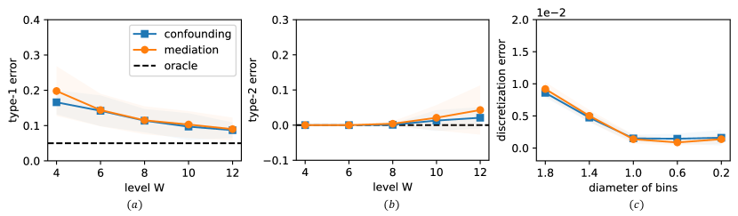
Figure 3: (a,b) Type-I and type-II errors of our method under different bin numbers. (c) Discretization errors under different bin diameters.

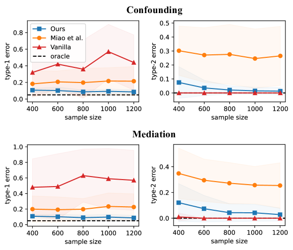
Figure 4: Type-I and type-II errors of our method and baselines under different sample sizes.

Influence of bin numbers. Fig. 3 shows the type-I and type-II errors of our method with bin numbers varying from $4$ to $12$. As we can see, the type-I error decreases and approaches the oracle level when $K$ increases. This is because when $K$ increases, the diameter of each bin becomes small. Under Asm. 4.6, this means the discretization error $\left|pr(Y|U\in B_{j})-pr(Y|U\in B_{j},X)\right|$ is close to an infinitesimal level (as shown in Fig. 3 (c)) and $\hat{Q}\sim\hat{q}$ has an approximate linear relation. Therefore, the test statistic $T$ converges to the chi-square distribution, and the type-I error is controlled. Besides, we can also observe that the type-II error is consistently small for different $K$s. This may be because the linear relation between $\hat{Q}$ and $\hat{q}$ is consistently broken by the causal edge $X\to Y$, no matter which bin number is used.

Comparison with baselines. Fig. 4 shows the type-I and type-II errors of our method and baselines. As shown, our method significantly outperforms the baselines. Specifically, compared with the vanilla method, our method can effectively control the type-I error, thanks to the proper use of the proxy variable; while the advantage over Miao et al. [5] can be attributed to the control of discretization error with the careful binning. In addition, we can also observe that our method comes close to the oracle performance when the sample size increases, which verifies our asymptotic theories in Thm. 2 and Cor. 4.9.

5.2 Treatment of sepsis disease

In this section, we apply our method to identify causal relations between two pairs of variables in sepsis disease:

1. $\text{Vancomycin}\to\text{White Blood Cell (WBC) count}$. The vancomycin is a common antibiotic [25, 26] used to control bacterial infection (measured by the WBC count) in patients with sepsis. According to an existing RCT [14], vancomycin can causally influence the WBC count.

2. $\text{Morphine}\not\to\text{WBC count}$. The prescription morphine is a common opioid medication used in pain management [11]. Clinically, the dosage of morphine appears a strong correlation with the WBC count [12]. However, according to a recent RCT [13], this correlation is highly likely to be confounding bias instead of causation.

For both cases, the latent confounder is the patient’s health status. To adjust for the confounding, we use blood pressure as the proxy variable.

Table 1: Identified causal relations in sepsis disease.

Method	Vancomycin$\to$ WBC	Morphine$\to$ WBC
Ground truth (RCT)	✓	✗
Vanilla	✓	✓
Miao et al.[5]	✗	✓
Ours	✓	✗

Data extraction. We consider the Medical Information Mart for Intensive Care (MIMIC III) [27] database, which consists of electronic health records from patients in the Intensive Care Unit (ICU). From MIMIC III, we extract 3251 patients that are diagnosed with sepsis during their stays. Among these, there are (resp.) 1888 and 559 patients with vancomycin and morphine records.

Results. Tab. 1 shows the identified causal relations of our method and baselines. As we can see, our method identifies causal relations that well align with the RCT findings in both cases, which demonstrates its effectiveness and utility. In contrast, there is a large discrepancy between the results given by baseline methods and the RCTs. For example, the vanilla method detects $\text{Morphine}\to\text{WBC}$, which can be a false positive result due to the failure of adjusting for the confounding bias. Miao et al. [5] gives inconsistent results in both cases, indicating that the proxy variable may lose its power without careful control of the discretization error.

6 Conclusion

In this paper, we propose a proxy-based method to identify causal relations when unobserved variables are present. Our method requires the discretization of continuous variables, for which we provide mild conditions to control the involved discretization error. Benefiting from this, our test enjoys a tractable type-I error and outperforms baselines in both synthetic and real data.

Limitation and future work. Our method relies on discretization and therefore may be affected by the dimension of the proxy variable. Indeed, the curse of dimensionality is a common issue faced by all conditional independence (CI) test methods [28, 29]. To alleviate this problem, we will investigate theories on high-dimensional CI test [30, 31] and discretization [32, Lem. 5.12] to pursue a delicate solution. Besides, we are also interested to plug our test into multi-variable causal discovery methods such as the Fast Causal Inference (FCI) algorithm [33], to enhance their identification ability.

Appendix A Controlling the discretization error

In this section, we introduce the proof of Thm. 4.2  and Exam. 4.4.

For the convenience of the mathematical derivation, we use the $L_{1}$-distance and the Total Variance (TV) distance interchangeably, since for two distributions $\mathcal{P},\mathcal{Q}$:

$$||\mathcal{P},\mathcal{Q}||_{1}:=\frac{1}{2}\int|p(x)-q(x)|dx=TV(\mathcal{P},\mathcal{Q}).$$

A.1 Proof of Thm. 4.2

Theorem 4.2. Suppose that $u\mapsto\mathcal{P}_{Y|X,U=u}$ and $u\mapsto\mathcal{P}_{Y|U=u}$ are (resp.) $L_{Y|X}$-Lipschitz and $L_{Y}$-Lipschitz with respect to $L_{1}$-distance. Suppose that $\{B_{j}\}_{j=1}^{J}$ is a measurable partition of $supp(U)$, and that for every bin $B_{j}$,

$$diam(B_{j})\leq\frac{1}{2}\min\{\epsilon/L_{Y},\epsilon/L_{Y|X}\}.$$

Suppose that $X\perp\!\!\!\!\perp Y|U$, then, we have:

$$\left|pr(y|U\in B_{j},x)-pr(y|U\in B_{j})\right|\leq\epsilon.$$

To prove Thm. 4.2, we first introduce the following lemma, which shows that if two distributions are close in $L_{1}$-distance, then their probability density values are also close.

Lemma A.1.

Consider two distributions $\mathcal{P},\mathcal{Q}$ over the random variable $X$, if $||\mathcal{P},\mathcal{Q}||_{1}\leq\epsilon$, then $\left|pr_{\mathcal{P}}(X\in A)-pr_{\mathcal{Q}}(X\in A)\right|\leq\epsilon$, for any set $A\in supp(X)$.

Proof.

The proof is immediate considering the fact that the $L_{1}$-distance equals the TV distance and the definition that:

$$TV(\mathcal{P},\mathcal{Q}):=\sup_{A}\left|pr_{\mathcal{P}}(X\in A)-pr_{\mathcal{Q}}(X\in A)\right|.$$

∎

We also require the following lemma, which connects the smoothness conditions to the closeness of distributions in $L_{1}$-distance.

Lemma A.2.

Suppose that $u\mapsto\mathcal{P}_{Y|U=u}$ be $L_{Y}$-Lipschitz with respect to $L_{1}$-distance. Suppose that $\{B_{j}\}_{j=1}^{J}$ is a measurable partition of $supp(U)$, and that $diam(B_{j})\leq\epsilon/L_{Y}$ for every bin $B_{j}$ in the partition. Then, for all $u_{0}\in B_{j}$, we have:

$$||\mathcal{P}_{Y|U=u_{0}},\mathcal{P}_{Y|U\in B_{j}}||_{1}\leq\epsilon.$$ (9)

Proof.

We first show that $\mathcal{P}_{Y|U\in B_{j}}$ can be written as:

$$\mathcal{P}_{Y|U\in B_{j}}=\mathchoice{{\vbox{\hbox{$\textstyle-$ }}\kern-7.83337pt}}{{\vbox{\hbox{$\scriptstyle-$ }}\kern-5.90005pt}}{{\vbox{\hbox{$\scriptscriptstyle-$ }}\kern-4.75003pt}}{{\vbox{\hbox{$\scriptscriptstyle-$ }}\kern-4.25003pt}}\!\int_{B_{j}}\mathcal{P}_{Y|U=u}d\mathcal{P}_{U}(u),$$ (10)

where $\mathchoice{{\vbox{\hbox{$\textstyle-$ }}\kern-7.83337pt}}{{\vbox{\hbox{$\scriptstyle-$ }}\kern-5.90005pt}}{{\vbox{\hbox{$\scriptscriptstyle-$ }}\kern-4.75003pt}}{{\vbox{\hbox{$\scriptscriptstyle-$ }}\kern-4.25003pt}}\!\int$ denotes the averaged integral over $B_{j}$, i.e., the integral divided by the measure on the integration domain $B_{j}$.

Specifically, for any Borel set $D\subseteq supp(Y)$, the left hand side of (10) is:

$$\mathcal{P}_{Y|U\in B_{j}}(D)=pr(Y\in D|U\in B_{j}),$$

while the right-hand side is:

$${\int_{B_{j}}\mathcal{P}_{Y|U=u}(D)d\mathcal{P}_{U}(u)}/{\mathcal{P}_{U}(B_{j})}=pr(Y\in D,U\in B_{j})/pr(U\in B_{j}).$$

Therefore, (10) holds according to Bayes’ theorem.

Second, due to the assumed Lipschitzness, for any $u,u_{0}\in B_{j}$, we have:

$$||\mathcal{P}_{Y|U=u_{0}},\mathcal{P}_{Y|U=u}||_{1}=\sup_{D}\left|\mathcal{P}_{Y|U=u_{0}}(D)-\mathcal{P}_{Y|U=u}(D)\right|\leq L_{Y}\left|u_{0}-u\right|\leq\epsilon.$$ (11)

Now, to prove (9), we hope to prove:

$$||\mathcal{P}_{Y|U=u_{0}},\mathcal{P}_{Y|U\in B_{j}})||_{1}=\sup_{D}\left|\mathcal{P}_{Y|U=u_{0}}(D)-\mathcal{P}_{Y|U\in B_{j}}(D)\right|\leq\epsilon.$$ (12)

Next, we prove (12) by (10) and (11). Specifically, note that for any $D\subseteq supp(Y)$, we have:

$$|\mathcal{P}_{Y|U=u_{0}}(D) -\mathcal{P}_{Y|U\in B_{j}}(D)|=\left|\mathcal{P}_{Y|U=u_{0}}(D)-\mathchoice{{\vbox{\hbox{$\textstyle-$ }}\kern-7.83337pt}}{{\vbox{\hbox{$\scriptstyle-$ }}\kern-5.90005pt}}{{\vbox{\hbox{$\scriptscriptstyle-$ }}\kern-4.75003pt}}{{\vbox{\hbox{$\scriptscriptstyle-$ }}\kern-4.25003pt}}\!\int_{B_{j}}\mathcal{P}_{Y|U=u}(D)d\mathcal{P}_{U}(u)\right|$$ # (10)

$$=\left|\mathchoice{{\vbox{\hbox{$\textstyle-$ }}\kern-7.83337pt}}{{\vbox{\hbox{$\scriptstyle-$ }}\kern-5.90005pt}}{{\vbox{\hbox{$\scriptscriptstyle-$ }}\kern-4.75003pt}}{{\vbox{\hbox{$\scriptscriptstyle-$ }}\kern-4.25003pt}}\!\int_{B_{j}}\mathcal{P}_{Y|U=u_{0}}(D)d\mathcal{L}_{U}(u)-\mathchoice{{\vbox{\hbox{$\textstyle-$ }}\kern-7.83337pt}}{{\vbox{\hbox{$\scriptstyle-$ }}\kern-5.90005pt}}{{\vbox{\hbox{$\scriptscriptstyle-$ }}\kern-4.75003pt}}{{\vbox{\hbox{$\scriptscriptstyle-$ }}\kern-4.25003pt}}\!\int_{B_{j}}\mathcal{P}_{Y|U=u}(D)d\mathcal{P}_{U}(u)\right| \text{\#}\mathchoice{{\vbox{\hbox{$\textstyle-$ }}\kern-7.83337pt}}{{\vbox{\hbox{$\scriptstyle-$ }}\kern-5.90005pt}}{{\vbox{\hbox{$\scriptscriptstyle-$ }}\kern-4.75003pt}}{{\vbox{\hbox{$\scriptscriptstyle-$ }}\kern-4.25003pt}}\!\int_{B_{j}}d\mathcal{P}_{U}(u)=1$$

$$\leq\mathchoice{{\vbox{\hbox{$\textstyle-$ }}\kern-7.83337pt}}{{\vbox{\hbox{$\scriptstyle-$ }}\kern-5.90005pt}}{{\vbox{\hbox{$\scriptscriptstyle-$ }}\kern-4.75003pt}}{{\vbox{\hbox{$\scriptscriptstyle-$ }}\kern-4.25003pt}}\!\int_{B_{j}}\left|\mathcal{P}_{Y|U=u_{0}}(D)-\mathcal{P}_{Y|U=u}(D)\right|d\mathcal{P}_{U}(u)$$ # Triangle inequity

$$\leq\mathchoice{{\vbox{\hbox{$\textstyle-$ }}\kern-7.83337pt}}{{\vbox{\hbox{$\scriptstyle-$ }}\kern-5.90005pt}}{{\vbox{\hbox{$\scriptscriptstyle-$ }}\kern-4.75003pt}}{{\vbox{\hbox{$\scriptscriptstyle-$ }}\kern-4.25003pt}}\!\int_{B_{j}}\epsilon\,d\mathcal{P}_{U}(u)=\epsilon.$$ # (11)

Since for any $D\subseteq supp(Y)$, $\left|\mathcal{P}_{Y|U=u_{0}}(D)-\mathcal{P}_{Y|U\in B_{j}}(D)\right|\leq\epsilon$, we have (12) holds, and hence prove the proposition. ∎

Analogously, we also have the following lemma.

Lemma A.3.

Suppose that $u\mapsto\mathcal{P}_{Y|X,U=u}$ be $L_{Y|X}$-Lipschitz with respect to $L_{1}$-distance. Suppose that $\{B_{j}\}_{i=1}^{I}$ is a measurable partition of $supp(U)$, and that $diam(B_{j})\leq\epsilon/L_{Y|X}$ for every bin $B_{j}$ in the partition. Then, for all $u_{0}\in B_{j}$, we have:

$$||\mathcal{P}_{Y|X,U=u_{0}},\mathcal{P}_{Y|X,U\in B_{j}}||_{1}\leq\epsilon.$$

Equipped with Lem. A.1, Lem. 9, and Lem. A.3, we now introduce the proof of Thm. 4.2.

Proof of Thm. 4.2.

According to the Lipschitzness of $u\mapsto\mathcal{P}_{Y|X,U=u}$ and Lem. A.3, we have:

$$||\mathcal{P}_{Y|X,U=u_{0}},\mathcal{P}_{Y|X,U\in B_{j}}||\leq\frac{1}{2}\epsilon.$$

According to Lem. A.1, this indicates $\left|pr(y|x,U=u_{0})-pr(y|x,U\in B_{j})\right|\leq\frac{1}{2}\epsilon$.

Under $X\perp\!\!\!\!\perp Y|U$, we have $pr(y|x,U=u_{0})=pr(y|U=u_{0})$. Hence, we have:

$$\left|pr(y|U=u_{0})-pr(y|x,U\in B_{j})\right|\leq\frac{1}{2}\epsilon.$$ (13)

Similarly, according to the Lipschitzness of $u\mapsto\mathcal{P}_{Y|U=u}$, we have:

$$\left|pr(y|U=u_{0})-pr(y|U\in B_{j})\right|\leq\frac{1}{2}\epsilon.$$ (14)

Combining (13) and (14) with the triangle inequity, we have:

$$\left|pr(y|U\in B_{j})-pr(y|x,U\in B_{j})\right|\leq$$

$$\left|pr(y|U\in B_{j})-pr(y|U=u_{0})\right|+\left|pr(y|U=u_{0})-pr(y|x,U\in B_{j})\right|\leq\epsilon.$$

∎

A.2 Proof of Exam. 4.4: ANMs that satisfy the Lipschitz continuity

Example 4.4. Suppose that $X\leftarrow U\to Y$ (similarly for $X\to U\to Y$) is an addictive noise model, that is, $X=h(U)+N$ and $Y=g(U)+E$, where $N,E$ are exogenous noises. Denote the probability density function of $E$ as $f_{E}$. Then, the functions $u\mapsto\mathcal{P}_{Y|U=u,X}$ and $u\mapsto\mathcal{P}_{Y|U=u}$ are Lipschitz continuous with respect to $L_{1}$-distance if:

1. $g$ and $f_{E}$ are continuous and differentiable, and

2. $f_{E}^{\prime}$ is absolute integral, i.e. $\int|f_{E}^{\prime}(e)|de$ exists.

The second condition can be satisfied by, for example, the exponential family $E\sim exp$.

Proof.

Under $X\perp\!\!\!\!\perp Y|U$, we have $\mathcal{P}_{Y|X,U=u}=\mathcal{P}_{Y|U=u}$. Hence, it is suffice to show the Lipschitzness of $u\mapsto\mathcal{P}_{Y|U=u}$.

Specifically, we hope to prove $\forall u_{1},u_{2}\in supp(U)$:

$$||\mathcal{P}_{Y|U=u_{1}},\mathcal{P}_{Y|U=u_{2}})||_{1}\leq L_{Y}\left|u_{1}-u_{2}\right|.$$ (15)

We first re-write (15) with the structural function $g$ and probability density function $f_{E}$.

Specifically, the $L_{1}$-distance can be re-written as the $L_{1}$-distance between the probability density functions:

$$||\mathcal{P}_{Y|U=u_{1}},\mathcal{P}_{Y|U=u_{2}}||_{1}=\frac{1}{2}\int\left|f_{Y|U=u_{1}}(y)-f_{Y|U=u_{2}}(y)\right|dy.$$

We also have:

$$f_{Y|U=u}(y)=f_{E}(y-g(u)),$$

by inversing the structural equation $Y=g(U)+E$.

As a result, (15) can be re-written as: $\forall u_{1},u_{2}\in supp(U)$,

$$\int\left|f_{E}(y-g(u_{1}))-f_{E}(y-g(u_{2}))\right|dy\leq 2L_{y}\left|u_{1}-u_{2}\right|.$$ (16)

Next, we show (16) is true if:

1. $g$ and $f_{E}$ are continuous and differentiable,

2. $f_{E}^{\prime}$ is absolute integrable, i.e. $\int f_{E}^{\prime}(e)de$ exists.

Applying the Mean Value Theoremon the function $u\mapsto f_{E}(y-g(u))$, we have $\exists u_{c}\in(u_{1},u_{2})$ s.t.

$$\left|f_{E}(y-g(u_{1}))-f_{E}(y-g(u_{2}))\right|=\left|f_{E}^{\prime}(y-g(u_{c}))g^{\prime}(u_{c})\right|\cdot\left|u_{1}-u_{2}\right|$$

In this regard, we have:

$$\int\left|f_{E}(y-g(u_{1}))-f_{E}(y-g(u_{2}))\right|dy=|g^{\prime}(u_{c})|\int|f^{\prime}_{E}(y-g(u_{c}))|dy\left|u_{1}-u_{2}\right|.$$

Let $L_{Y}:=|g^{\prime}(u_{c})|\int|f^{\prime}_{E}(y-g(u_{c}))|dy$, we have:

$$\int\left|f_{E}(y-g(u_{1}))-f_{E}(y-g(u_{2}))\right|dy\leq 2L_{y}\left|u_{1}-u_{2}\right|,$$

hence, the Lipschitzness is proved.

∎

Appendix B Hypothesis test with asymptotic validity

B.1 Proof of Thm. 4.8: Asymptotic validity

Theorem 4.8. Assume models (a)-(b), Asm. 4.1, and Asms. 4.6-4.7. Discretize $X,W$ to $I,K(I\!>\!K)$ levels with sufficient fine bins. Denote the level difference as $r:=I-K$, the maximal bin diameter as $m$, and the sample size as $n$. If  $\mathbb{H}_{0}\!:\!X\perp\!\!\!\!\perp Y|U$ is correct, then $T_{y}\!\to\chi^{2}_{r}$ in distribution when $m\to 0,n\to\infty$.

Proof.

According to the law of total probability, we first have:

$$pr(W\in C_{k}|x)=\sum_{j}pr(W\in C_{k}|U\in B_{j},x)pr(U\in B_{j}|x).$$

In the form of the transition matrix, this means:

$${P}(\tilde{W}|x)={P}(\tilde{W}|\tilde{U},x){P}(\tilde{U}|x).$$ (17)

We also have:

$${pr}(y|x)=\sum_{j}{pr}(y|U\in B_{j},x){pr}(U\in B_{j}|x).$$

In the form of the transition matrix, this means:

$${pr}(y|x)={P}(y|\tilde{U},x){P}(\tilde{U}|x).$$ (18)

Under Asm. 4.1, (17) can be rewritten as:

$${P}(\tilde{W}|\tilde{U},x)^{-1}{P}(\tilde{W}|x)={P}(\tilde{U}|x).$$ (19)

(18) and (19) together give:

$${pr}(y|x)={P}(y|\tilde{U},x){P}(\tilde{W}|\tilde{U},x)^{-1}{P}(\tilde{W}|x).$$ (20)

The idea is that, under Asm. 4.6  and $\mathbb{H}_{0}\!:\!X\perp\!\!\!\!\perp Y|U$, we have ${P}(y|\tilde{U},x)\approx{P}(y|\tilde{U})$ by Thm. 4.2.

In addition, under model (a)-(b) ($X\perp\!\!\!\!\perp W|U$), we also have ${P}(\tilde{W}|\tilde{U},x)\approx{P}(\tilde{W}|\tilde{U})$.

Therefore, we have (informally):

$$pr(y|x)\approx{P}(y|\tilde{U}){P}(\tilde{W}|\tilde{U})^{-1}{P}(\tilde{W}|x).$$

This means under $\mathbb{H}_{0}$, $pr(y|x)$ has a linear relationship with $P(\tilde{W}|x)$, for fixed $y$, as $x$ varies. Therefore, any evidence against the linearity is evidence against $\mathbb{H}_{0}$.

Formally speaking, rewrite (20) as:

$$\,\,pr(y|x)$$

$$=\left[{P}(y|\tilde{U})+{P}(y|\tilde{U},x)-{P}(y|\tilde{U})\right]\left[{P}(\tilde{W}|\tilde{U})^{-1}+{P}(\tilde{W}|\tilde{U},x)^{-1}-{P}(\tilde{W}|\tilde{U})^{-1}\right]{P}(\tilde{W}|x)$$

$$={P}(y|\tilde{U}){P}(\tilde{W}|\tilde{U})^{-1}{P}(\tilde{W}|x)+\Delta{P}(\tilde{W}|x),$$ (21)

where

$$\Delta =\mathbb{P}(y|\tilde{U})\left[\mathbb{P}(\tilde{W}|\tilde{U},x)^{-1}-\mathbb{P}(\tilde{W}|\tilde{U})^{-1}\right]+\left[\mathbb{P}(y|\tilde{U},x)-\mathbb{P}(y|\tilde{U})\right]\mathbb{P}(\tilde{W}|\tilde{U})^{-1}$$

$$+\left[\mathbb{P}(y|\tilde{U},x)-\mathbb{P}(y|\tilde{U})\right]\left[\mathbb{P}(\tilde{W}|\tilde{U},x)^{-1}-\mathbb{P}(\tilde{W}|\tilde{U})^{-1}\right].$$

Since $X\perp\!\!\!\!\perp W|U$, Asm. 4.6  and Thm. 4.2 , we have:

$$\lim_{\epsilon\to 0}{P}(\tilde{W}|\tilde{U},x)-{P}(\tilde{W}|\tilde{U})=[0],$$

where $[0]$ denote the zero matrix. Since matrix inversion $F(M):M\mapsto M^{-1}$ is a continuous function, we have:

$$\lim_{\epsilon\to 0}{P}(\tilde{W}|\tilde{U},x)^{-1}-{P}(\tilde{W}|\tilde{U})^{-1}=[0],$$ (22)

Under $\mathbb{H}_{0}:X\perp\!\!\!\!\perp Y|U$, we also have:

$$\lim_{\epsilon\to 0}{P}(y|\tilde{U},x)-{P}(y|\tilde{U})=[0].$$ (23)

With (22) and (23), we have:

$$\lim_{\epsilon\to 0}\Delta =[0],$$

$$\lim_{\epsilon\to 0}{P}(y|x) ={P}(y|\tilde{U}){P}(\tilde{W}|\tilde{U})^{-1}{P}(\tilde{W}|x).$$

Considering all bins of $supp(X)$, this can be written in the form of the transition matrix:

$$\lim_{\epsilon\to 0}q_{y}^{T}={P}(y|\tilde{U}){P}(\tilde{W}|\tilde{U})^{-1}Q,$$ (24)

which means $q_{y}^{T}\sim Q$ (as $x$ varies) is linear under $\mathbb{H}_{0}$.

In the following, we discuss the asymptotic distribution of $n^{\frac{1}{2}}\xi_{y}$ and $T_{y}$.

We first show that $n^{\frac{1}{2}}\xi_{y}\to N(0,\Omega_{y})$ in distribution when $n\to\infty$ and $\epsilon\to 0$. Specifically, given that $\hat{Q}\to Q$, $\hat{\Sigma}_{y}\to\Sigma_{y}$ in probability and $n^{\frac{1}{2}}(\hat{q}_{y}-q_{y})\to N(0,\Sigma_{y})$ in distribution, applying Slutsky’s theorem, we have $n^{\frac{1}{2}}(\xi_{y}-\Omega_{y}\Sigma_{y}^{-\frac{1}{2}}q_{y})\to N(0,\Omega_{y})$ in distribution with $\Omega_{y}=I-{\Sigma}_{y}^{-\frac{1}{2}}{Q}^{T}({Q}{\Sigma}_{y}^{-1}{Q}^{T})^{-1}{Q}{\Sigma}_{y}^{-\frac{1}{2}}$. If $\mathbb{H}_{0}$ is correct, by (24), we have $\Omega_{y}\Sigma_{y}^{-\frac{1}{2}}q_{y}\to 0$, which, by applying Slutsky’s theorem again, implies that $n^{\frac{1}{2}}\xi_{y}\to N(0,\Omega_{y})$ in distribution.

Next, we show that $\Omega_{y}$ has rank $r=I-K$. Specifically, the rank of $Q$ is $K$ by Asm. 4.7 . Because multiplying an invertible matrix does not change the rank of the matrix, the rank of $Q\Sigma_{y}^{-\frac{1}{2}}$ is $K$. Since transposing a matrix does not change its rank, the rank of the idempotent matrix ${\Sigma}_{y}^{-\frac{1}{2}}{Q}^{T}({Q}{\Sigma}_{y}^{-1}{Q}^{T})^{-1}{Q}{\Sigma}_{y}^{-\frac{1}{2}}$ is also $K$. By Corollary 11.5 of [34], the matrix ${\Sigma}_{y}^{-\frac{1}{2}}{Q}^{T}({Q}{\Sigma}_{y}^{-1}{Q}^{T})^{-1}{Q}{\Sigma}_{y}^{-\frac{1}{2}}$ has $K$ eigenvalues equal to one and $I-K$ eigenvalues equal to zero. Hence, $\Omega_{y}$ is an idempotent matrix with rank $r=I-K$.

Finally, we show that the test statistic $T_{y}:=n^{\frac{1}{2}}\xi_{y}^{T}\xi_{y}$ has an asymptotic chi-square distribution with freedom $r$.

We first introduce a theorem about the asymptotic distribution of a random variable $X$ and the random variable $X^{T}X$. According to Thm. 1.12 of [35], if $X\to Y$ in distribution, then $nX^{T}X\to Y^{T}Y$ in distribution. Now, let $X$ be $n^{\frac{1}{2}}$ and $Y$ be $N(0,\Omega_{y})$, we have:

$$T_{y}:=n\xi_{y}^{T}\xi_{y}\to N(0,\Omega_{y})^{T}N(0,\Omega_{y})\,\,\text{in distribution}.$$

We then explain why $N(0,\Omega_{y})^{T}N(0,\Omega_{y})=\chi^{2}_{r}$. Because $\Omega_{y}$ is a symmetric matrix, we can find an orthogonal matrix $V$ such that $V\Omega_{y}V^{T}=diag(1,...,1,0,...,0)$, a diagonal matrix with $r$ $1$s and $I-r$ $0$s in the diagonal. Hence, we have $VN(0,\Omega_{y})\sim N(0,diag(1,...,1,0,...,0))$ and,

$$N(0,\Omega_{y})^{T}N(0,\Omega_{y})=\left[VN(0,\Omega_{y})\right]^{T}\left[VN(0,\Omega_{y})\right]=\chi^{2}_{r}.$$

∎

Appendix C Empirical estimation method

In this section, we provide the empirical estimation method to obtain estimators that satisfy the asymptotic properties:

$$n^{\frac{1}{2}}(\hat{q}_{y}-q_{y}) \to N(0,\Sigma_{y})\,\,\text{in distribution},$$

$$\hat{Q}\to Q\,\,\text{and}\,\,\hat{\Sigma}_{y}\to\Sigma_{y}\,\, \text{in probability},\,\,\text{with $\hat{\Sigma}_{y},\Sigma_{y}$ positive-definite}.$$

We start from the univariate case for illustration.

Univariate case. Consider a discrete random variable $X$ that takes $k$ levels of values $\{x_{1},x_{2},...,x_{k}\}$. For $n$ iid samples $\{X_{1},X_{2},...,X_{n}\}$, let $Z_{i}$ be the number of samples that take the value $x_{i}$. Then, we have $\mathbf{Z}:=\{Z_{1},Z_{2},...,Z_{k}\}^{T}$ follows a multinomial distribution with parameters $(n,\mathbf{p})$, where $\mathbf{p}:=\{pr(x_{1}),pr(x_{2}),...,pr(x_{k})\}^{T}$. In the following, we use $p_{i}$ to denote $pr(x_{i})$ for simplicity.

Our objective is to compute the Maximum Likelihood Estimator (MLE) $\hat{\mathbf{p}}:=\{\hat{p}_{1},...,\hat{p}_{k}\}^{T}$ of $\mathbf{p}$, which enjoys the asymptotic properties.

For this purpose, we first write the joint probability mass function for $n$ sample:

$$f_{n}(z_{1},z_{2},...,z_{k}|n,\mathbf{p})=n!\prod_{i=1}^{k}\frac{p_{i}^{z_{i}}}{z_{i}!}.$$

Then, the log-likelihood is:

$$h_{n}(p_{1},p_{2},...,p_{k},n|\mathbf{z}):=log(f(z_{1},z_{2},...,z_{k}|n,\mathbf{p}))=log(n!)+\sum_{i=1}^{k}z_{i}log(p_{i})-\sum_{i=1}^{k}z_{i}!.$$

To obtain the MLE estimator $\hat{\mathbf{p}}$, we maximize $h_{n}(\mathbf{p})$, with $p_{1}+p_{2}+...+p_{k}=1$ as the constraint. This can be converted to an unconstrained optimization problem by a Lagrange multiplier:

$$\arg\max_{p_{1},p_{2},...,p_{k}}l_{n}(p_{1},p_{2},...,p_{k}):=h_{n}(p_{1},p_{2},...,p_{k},n)+\lambda(1-\sum_{i=1}^{k}p_{i}).$$

The derivative $\bigtriangledown l_{n}(\mathbf{p})$ is:

$$\bigtriangledown l_{n}(\mathbf{p})=[\frac{\partial l_{n}}{\partial p_{1}},...,\frac{\partial l_{n}}{\partial p_{k}}]^{T}=[\frac{z_{i}}{p_{i}}-\lambda,...,\frac{z_{k}}{p_{k}}-\lambda]^{T}.$$

Let $\bigtriangledown l_{n}(\mathbf{p})=\mathbf{0}$ and considering $\sum_{i}^{k}p_{i}^{*}=1$, we have $p_{i}^{*}=\frac{z_{i}}{n},\lambda=n$.

Therefore, the MLE estimator is $\mathbf{\hat{p}}=\{\frac{Z_{1}}{n},...,\frac{Z_{k}}{n}\}$. The covariance matrix of $\mathbf{\hat{p}}$ can be computed by definition:

$$\mathrm{Cov}[\mathbf{\hat{p}}]=\frac{1}{n}\begin{bmatrix}p_{1}(1-p_{1})&-p_{1}p_{2}&...&-p_{1}p_{k}\\ -p_{2}p_{1}&p_{2}(1-p_{2})&...&-p_{2}p_{k}\\ \vdots&\vdots&&\vdots\\ -p_{k}p_{1}&-p_{k}p_{2}&...&p_{k}(1-p_{k})\end{bmatrix}.$$ (25)

Another way to compute the covariance matrix is to use the Fisher information. Specifically, the Taylor expansion of $\bigtriangledown l_{n}(\mathbf{p})$ at $\mathbf{p}_{0}$ (the ground-truth parameter) is:

$$\bigtriangledown l_{n}(\mathbf{p})=\bigtriangledown l_{n}(\mathbf{p}_{0})+[\bigtriangledown^{2}l_{n}(\mathbf{p}_{0})]^{T}(\mathbf{p}-\mathbf{p}_{0})+o(\mathbf{p}),$$

where $\bigtriangledown l_{n}(\mathbf{p})=[\frac{z_{1}}{p_{1}}-n,...,\frac{z_{k}}{p_{k}}-n]^{T}$, $\bigtriangledown^{2}l_{n}(\mathbf{p})=-\mathrm{diag}[\frac{z_{1}}{p_{1}^{2}},...,\frac{z_{k}}{p_{k}^{2}}]$.

Let $\mathbf{p}=\mathbf{\hat{p}}$, considering the Hessian matrix $\bigtriangledown^{2}l_{n}(\mathbf{p})$ is symmetric for any $\mathbf{p}$, we have:

$$\sqrt{n}(\mathbf{\hat{p}}-\mathbf{p}_{0})=(-\frac{1}{n}\bigtriangledown^{2}l_{n}(\mathbf{p}_{0}))^{-1}(\frac{1}{\sqrt{n}}\bigtriangledown l_{n}(\mathbf{p}_{0})).$$

Since the multinomial is defined on iid samples, and we have $l_{n}(\mathbf{p})=\sum_{i}^{n}l_{i}(\mathbf{p})$, we can view $l_{n}(\mathbf{p})$ and its derivative as the summation of iid random vectors. Thus, by the law of large numbers and central limit (in the matrix form), we have (by noting that $\mathrm{E}[\bigtriangledown l_{1}(\mathbf{p}_{0})])=0$):

$$-\frac{1}{n}\bigtriangledown^{2}l_{n}(\mathbf{p}_{0}) \to-\mathrm{E}[\bigtriangledown^{2}l_{1}(\mathbf{p}_{0})]\,\,\text{in probability},$$

$$\frac{1}{\sqrt{n}}\bigtriangledown l_{n}(\mathbf{p}_{0})=\sqrt{n}(\frac{1}{n}\bigtriangledown l_{n}(\mathbf{p}_{0}) -\mathrm{E}[\bigtriangledown l_{1}(\mathbf{p}_{0})])\to N(\mathbf{0},\mathrm{Var}[\bigtriangledown l_{1}(\mathbf{p}_{0})])\,\,\text{in distribution}.$$

Let $J_{n}(\mathbf{p}):=-\mathrm{E}[\bigtriangledown^{2}l_{n}(\mathbf{p})]$, $V_{n}(\mathbf{p}):=\mathrm{Var}[\bigtriangledown l_{n}(\mathbf{p})]$, we then have:

$$\sqrt{n}(\mathbf{\hat{p}}-\mathbf{p}_{0})\to N(\mathbf{0},J_{1}(\mathbf{p}_{0})^{-1}V_{1}(\mathbf{p}_{0})J_{1}(\mathbf{p}_{0})^{-1})\,\,\text{in distribution},$$

where $J_{1}(\mathbf{p}_{0})=-\frac{1}{n}\mathrm{E}[\bigtriangledown^{2}l_{n}(\mathbf{p}_{0})]=-\mathrm{diag}\{\frac{1}{p_{1}},...,\frac{1}{p_{k}}\}$, and

$$V_{1}(\mathbf{p}_{0})=\frac{1}{n}\mathrm{Var}[\bigtriangledown l_{n}(\mathbf{p}_{0})]=\begin{bmatrix}\frac{1-p_{1}}{p_{1}}&-1&...&-1\\ -1&\frac{1-p_{2}}{p_{2}}&...&-1\\ \vdots&\vdots&&\vdots\\ -1&-1&...&\frac{1-p_{k}}{p_{k}}\end{bmatrix}.$$

Note that the asymptotic covariance $J_{1}(\mathbf{p}_{0})^{-1}V_{1}(\mathbf{p}_{0})J_{1}(\mathbf{p}_{0})^{-1}$ is consistent with the result in (25). Also note that $J_{1}$ no longer equals to $V_{1}$, that is, the Fisher information matrix has a “sandwich” form.

Bivariate case. Consider two discrete random variables $X,Y$, which (resp.) take $k,l$ levels of values $\{x_{1},...,x_{k}\}$ and $\{y_{1},...,y_{l}\}$. For $n$ iid samples $\{(X_{1},Y_{1}),...,(X_{n},Y_{n})\}$, let $Z_{ij}$ be the number of samples that take the value $(x_{i},y_{j})$. Then, we have $\mathbf{Z}:=\{Z_{ij}\}_{ij}^{T}$ follows the multinomial distribution with parameters $(n,\mathbf{p})$, where $\mathbf{p}:=\{pr(x_{i},y_{j})\}_{ij}=\{pr(x_{i})pr(y_{j}|x_{i})\}_{ij}$.

To obtain the MLE estimator $\mathbf{\hat{p}}=[\{\hat{p}(x_{i})\}_{i},\{\hat{p}(y_{j}|x_{i})\}_{ij}]^{T}$, we again write the log-likelihood function for $n$ samples:

$$h_{n}(\mathbf{p})=log(n!)+\sum_{i,j}z_{ij}log(p(y_{j}|x_{i})+\sum_{i,j}z_{ij}log(p(x_{i}))-\sum_{i,j}log(z_{ij}!).$$ (26)

To obtain $\hat{\mathbf{p}}$, we maximize $h_{n}(\mathbf{p})$, with the following $k+1$ constraints: $\sum_{j}p(y_{j}|x_{i})=1$ for $i=1,2,...,k$, and $\sum_{i}p(x_{i})=1$. This can be converted to the following unconstrained optimization problem:

$$\arg\max_{\mathbf{p}}l_{n}(\mathbf{p}):=h_{n}(\mathbf{p})+\lambda_{1}(1-\sum_{j}p(y_{j}|x_{1}))+...+\lambda_{k}(1-\sum_{j}p(y_{j}|x_{k}))+\lambda_{k+1}(1-\sum_{i}p(x_{i})).$$

Let the derivative $\bigtriangledown l_{n}(\mathbf{p})=[\{\frac{Z_{i:}}{p(x_{i})}-\lambda_{k+1}\}_{i},\{\frac{Z_{ij}}{p(y_{j}|x_{i})}-\lambda_{i}\}_{ij}]^{T}=\mathbf{0}$, where $Z_{i:}:=\sum_{j}Z_{ij}$, we have $\lambda_{i}=Z_{i:},\lambda_{k+1}=n$, and the MLE estimator $\mathbf{\hat{p}}=[\{\hat{p}(x_{i})\}_{i},\{\hat{p}(y_{j}|x_{i})\}_{ij}]^{T}$, where $\hat{p}(x_{i})=\frac{Z_{i:}}{n},\hat{p}(y_{j}|x_{i})=\frac{Z_{ij}}{Z_{i:}}$.

In the following, we compute the covariance matrix of $\hat{\mathbf{p}}$ with the Fisher information. Specifically, we need to compute the matrices $J_{1}(\mathbf{p}_{0})$ and $V_{1}(\mathbf{p}_{0})$.

The first and second order derivative of $l_{n}(\mathbf{p})$ are (resp.):

$$\bigtriangledown l_{n}(\mathbf{p}) =[\{\frac{Z_{i:}}{p(x_{i})}-n\}_{i},\{\frac{Z_{ij}}{p(y_{j}|x_{i})}-Z_{i:}\}_{ij}]_{(k+kl)\times 1}^{T}$$

$$\bigtriangledown^{2}l_{n}(\mathbf{p}) =\mathrm{diag}[\{\frac{Z_{i:}}{p(x_{i})^{2}}\}_{i},\{-\frac{Z_{ij}}{p(y_{j}|x_{i})^{2}}\}_{ij}]_{(k+kl)\times(k+kl)}.$$

Hence, $J_{n}(\mathbf{p})=-\mathrm{E}[\bigtriangledown^{2}l_{n}(\mathbf{p})]=n\mathrm{diag}[\{\frac{1}{p(x_{i})}\}_{i},\{\frac{p(x_{i})}{p(y_{j}|x_{i})}\}_{ij}]$.

By definition, we have $V_{n}(\mathbf{p})=\mathrm{Var}[\bigtriangledown l_{n}(\mathbf{p})]$, which involves the following terms (obtained by simple calculus and the fact that $\mathrm{Cov}(A+B,C)=\mathrm{Cov}(A,C)+\mathrm{Cov}(B,C)$):

$$\mathrm{Var}[\frac{Z_{i:}}{p(x_{i})}-n]=n\,\frac{1-p(x_{i})}{p(x_{i})}$$

$$\mathrm{Var}[\frac{Z_{ij}}{p(y_{j}|x_{i})}-Z_{i:}]=n\,\frac{p(x_{i})(1-p(y_{j}|x_{i}))}{p(y_{j}|x_{i})}$$

$$\mathrm{Cov}[\frac{Z_{i1:}}{p(x_{i1})}-n,\frac{Z_{i2:}}{p(x_{i2})}-n]=-n$$

$$\mathrm{Cov}[\frac{Z_{i1j1}}{p(y_{j}1|x_{i}1)}-Z_{i1:},\frac{Z_{i2j2}}{p(y_{j}2|x_{i}2)}-Z_{i2:}]=0$$

$$\mathrm{Cov}[\frac{Z_{i1:}}{p(x_{i1})}-n,\frac{Z_{i2j}}{p(y_{j}|x_{i}2)}-Z_{i2:}]=0.$$

Therefore, for $\mathbf{\hat{p}}=\{\hat{p}(x_{1}),...,\hat{p}(x_{k}),\hat{p}(y_{1}|x_{1}),...,\hat{p}(y_{l}|x_{1}),...,\hat{p}(y_{1}|x_{k}),\hat{p}(y_{l}|x_{k})\}^{T}$, we have:

$$\sqrt{n}(\mathbf{\hat{p}}-\mathbf{p}_{0})\to_{D}N(\mathbf{0},J_{1}(\mathbf{p}_{0})^{-1}V_{1}(\mathbf{p}_{0})J_{1}(\mathbf{p}_{0})^{-1}),$$

where:

$$J_{1}(\mathbf{p}_{0})^{-1}=\mathrm{diag}[\underbrace{p(x_{1}),p(x_{2}),...,p(x_{k})}_{k},\underbrace{\frac{p(y_{1}|x_{1})}{p(x_{1})},...,\frac{p(y_{l}|x_{1})}{p(x_{1})},...,\frac{p(y_{1}|x_{k})}{p(x_{k})},...,\frac{p(y_{l}|x_{k})}{p(x_{k})}}_{k\times l}],$$

and

$$V_{1}(\mathbf{p}_{0})=\begin{bmatrix}A&[0]_{k\times kl}\\ [0]_{kl\times k}&\mathrm{diag}\{a_{11},a_{12},...,a_{kl}\}_{kl\times kl}\end{bmatrix},$$

with

$$A=\begin{bmatrix}\frac{1-p(x_{1})}{p(x_{1})}&-1&...&-1\\ -1&\frac{1-p(x_{2})}{p(x_{2})}&...&-1\\ \vdots&\vdots&&\vdots\\ -1&-1&...&\frac{1-p(x_{k})}{p(x_{k})}\end{bmatrix}_{k\times k}.$$

Therefore, $J_{1}(\mathbf{p}_{0})^{-1}V_{1}(\mathbf{p}_{0})J_{1}(\mathbf{p}_{0})^{-1}$ is:

$$\begin{bmatrix}B&[0]_{k\times kl}\\ [0]_{kl\times k}&\mathrm{diag}\{a_{11}b_{11}^{2},a_{12}b_{12}^{2},...,a_{kl}b_{kl}^{2}\}_{kl\times kl}\end{bmatrix},$$

with

$$B=\begin{bmatrix}p(x_{1})(1-p(x_{1}))&-p(x_{1})p(x_{2})&...&-p(x_{1})p(x_{k})\\ -p(x_{2})p(x_{1})&p(x_{2})(1-p(x_{2}))&...&-p(x_{2})p(x_{k})\\ \vdots&\vdots&&\vdots\\ -p(x_{k})p(x_{1})&-p(x_{k})p(x_{1})&...&p(x_{k})(1-p(x_{k}))\end{bmatrix}_{k\times k}.$$

and

$$a_{ij}=\frac{p(x_{i})(1-p(y_{j}|x_{i}))}{p(y_{j}|x_{i})},b_{ij}=\frac{p(y_{j}|x_{i})}{p(x_{i})}.$$

In addition, according to the marginal property of the multinomial distribution, the asymptotic normality covariance $\Sigma_{y}$ of the estimator $\hat{q}_{y_{j}}=[\hat{p}(y_{j}|x_{1}),...,\hat{p}(y_{j}|x_{k})]^{T}=[\frac{Z_{1j}}{Z_{1:}},...,\frac{Z_{kj}}{Z_{k:}}]^{T}$ is:

$$\Sigma_{y}=\mathrm{diag}\{a_{1j}b_{1j}^{2},...,a_{kj}b_{kj}^{2}\}=\mathrm{diag}[\frac{p(y_{j}|x_{1})(1-p(y_{j}|x_{1}))}{p(x_{1})},...,\frac{p(y_{j}|x_{k})(1-p(y_{j}|x_{k}))}{p(x_{k})}],$$

whose consistent estimator $\hat{\Sigma}_{y}$ can be obtained by replacing $p$ with $\hat{p}$.

References

• [1] KJ Jager, C Zoccali, A Macleod, and FW Dekker. Confounding: what it is and how to deal with it. Kidney international, 73(3):256–260, 2008.
• [2] Raymond Hicks and Dustin Tingley. Causal mediation analysis. The Stata Journal, 11(4):605–619, 2011.
• [3] Kenneth J Rothman, Sander Greenland, Timothy L Lash, et al. Modern epidemiology, volume 3. Wolters Kluwer Health/Lippincott Williams & Wilkins Philadelphia, 2008.
• [4] Manabu Kuroki and Judea Pearl. Measurement bias and effect restoration in causal inference. Biometrika, 101(2):423–437, 2014.
• [5] Wang Miao, Zhi Geng, and Eric J Tchetgen Tchetgen. Identifying causal effects with proxy variables of an unmeasured confounder. Biometrika, 105(4):987–993, 2018.
• [6] Eric J Tchetgen Tchetgen, Andrew Ying, Yifan Cui, Xu Shi, and Wang Miao. An introduction to proximal causal learning. arXiv preprint arXiv:2009.10982, 2020.
• [7] Eric Tchetgen Tchetgen, Chan Park, and David Richardson. Single proxy control. arXiv e-prints, pages arXiv–2302, 2023.
• [8] Eric Tchetgen Tchetgen. The control outcome calibration approach for causal inference with unobserved confounding. American journal of epidemiology, 179(5):633–640, 2014.
• [9] Huan Liu, Farhad Hussain, Chew Lim Tan, and Manoranjan Dash. Discretization: An enabling technique. Data mining and knowledge discovery, 6:393–423, 2002.
• [10] Dimitris Margaritis. Distribution-free learning of bayesian network structure in continuous domains. In AAAI, volume 5, pages 825–830, 2005.
• [11] Henry McQuay. Opioids in pain management. The Lancet, 353(9171):2229–2232, 1999.
• [12] Rui Zhang, Jingjing Meng, Qinshu Lian, Xi Chen, Brent Bauman, Haitao Chu, Bradley Segura, and Sabita Roy. Prescription opioids are associated with higher mortality in patients diagnosed with sepsis: a retrospective cohort study using electronic health records. PLoS One, 13(1):e0190362, 2018.
• [13] KJS Anand, R Whit Hall, Nirmala Desai, Barbara Shephard, Lena L Bergqvist, Thomas E Young, Elaine M Boyle, Ricardo Carbajal, Vinod K Bhutani, Mary Beth Moore, et al. Effects of morphine analgesia in ventilated preterm neonates: primary outcomes from the neopain randomised trial. The Lancet, 363(9422):1673–1682, 2004.
• [14] Jamie M Rosini, Julie Laughner, Brian J Levine, Mia A Papas, John F Reinhardt, and Neil B Jasani. A randomized trial of loading vancomycin in the emergency department. Annals of Pharmacotherapy, 49(1):6–13, 2015.
• [15] Christos Louizos, Uri Shalit, Joris M Mooij, David Sontag, Richard Zemel, and Max Welling. Causal effect inference with deep latent-variable models. Advances in neural information processing systems, 30, 2017.
• [16] Ben Deaner. Many proxy controls. arXiv preprint arXiv:2110.03973, 2021.
• [17] Afsaneh Mastouri, Yuchen Zhu, Limor Gultchin, Anna Korba, Ricardo Silva, Matt Kusner, Arthur Gretton, and Krikamol Muandet. Proximal causal learning with kernels: Two-stage estimation and moment restriction. In International Conference on Machine Learning, pages 7512–7523. PMLR, 2021.
• [18] Wang Miao, Wenjie Hu, Elizabeth L Ogburn, and Xiao-Hua Zhou. Identifying effects of multiple treatments in the presence of unmeasured confounding. Journal of the American Statistical Association, pages 1–15, 2022.
• [19] Lu Cheng, Ruocheng Guo, and Huan Liu. Causal mediation analysis with hidden confounders. In Proceedings of the Fifteenth ACM International Conference on Web Search and Data Mining, pages 113–122, 2022.
• [20] Judea Pearl. Causality. Cambridge university press, 2009.
• [21] Tzee-Ming Huang. Testing conditional independence using maximal nonlinear conditional correlation. 2010.
• [22] Matey Neykov, Sivaraman Balakrishnan, and Larry Wasserman. Minimax optimal conditional independence testing. The Annals of Statistics, 49(4):2151–2177, 2021.
• [23] Andrew Warren. Wasserstein conditional independence testing. arXiv preprint arXiv:2107.14184, 2021.
• [24] Kun Zhang, Jonas Peters, Dominik Janzing, and Bernhard Schölkopf. Kernel-based conditional independence test and application in causal discovery. arXiv preprint arXiv:1202.3775, 2012.
• [25] Robert C Moellering Jr. Vancomycin: a 50-year reassessment, 2006.
• [26] Michael Rybak, Ben Lomaestro, John C Rotschafer, Robert Moellering Jr, William Craig, Marianne Billeter, Joseph R Dalovisio, and Donald P Levine. Therapeutic monitoring of vancomycin in adult patients: a consensus review of the american society of health-system pharmacists, the infectious diseases society of america, and the society of infectious diseases pharmacists. American Journal of Health-System Pharmacy, 66(1):82–98, 2009.
• [27] Alistair EW Johnson, Tom J Pollard, Lu Shen, Li-wei H Lehman, Mengling Feng, Mohammad Ghassemi, Benjamin Moody, Peter Szolovits, Leo Anthony Celi, and Roger G Mark. Mimic-iii, a freely accessible critical care database. Scientific data, 3(1):1–9, 2016.
• [28] Aaditya Ramdas, Sashank Jakkam Reddi, Barnabás Póczos, Aarti Singh, and Larry Wasserman. On the decreasing power of kernel and distance based nonparametric hypothesis tests in high dimensions. In Proceedings of the AAAI Conference on Artificial Intelligence, volume 29, 2015.
• [29] Rajen D Shah and Jonas Peters. The hardness of conditional independence testing and the generalised covariance measure. 2020.
• [30] Alexis Bellot and Mihaela van der Schaar. Conditional independence testing using generative adversarial networks. Advances in Neural Information Processing Systems, 32, 2019.
• [31] Ankur Ankan and Johannes Textor. A simple unified approach to testing high-dimensional conditional independences for categorical and ordinal data. arXiv preprint arXiv:2206.04356, 2022.
• [32] Ramon Van Handel. Probability in high dimension. Technical report, PRINCETON UNIV NJ, 2014.
• [33] Peter Spirtes, Clark N Glymour, Richard Scheines, and David Heckerman. Causation, prediction, and search. MIT press, 2000.
• [34] Sudipto Banerjee and Anindya Roy. Linear algebra and matrix analysis for statistics. Crc Press, 2014.
• [35] Jun Shao. Mathematical statistics. Springer Science & Business Media, 2003.