Boosting Visual-Language Models by Exploiting Hard Samples

Abstract

Large vision and language models, such as Contrastive Language-Image Pre-training (CLIP), are rapidly becoming the industry norm for matching images and texts. In order to improve its zero-shot recognition performance, current research either adds additional web-crawled image-text pairs or designs new training losses. However, the additional costs associated with training from scratch and data collection substantially hinder their deployment. In this paper, we present Helip, a low-cost strategy for boosting the performance of well-trained CLIP models by finetuning them with hard samples over original training data. Mixing hard examples into each batch, the well-trained CLIP model is then fine-tuned using the conventional contrastive alignment objective and a margin loss to distinguish between normal and hard negative data. Helip is deployed in a plug-and-play fashion to existing models. On a comprehensive zero-shot and retrieval benchmark, without training the model from scratch or utilizing additional data, Helip consistently boosts existing models to achieve leading performance. In particular, Helip boosts ImageNet zero-shot accuracy of SLIP by 3.05 and 4.47 when pretrained on CC3M and CC12M respectively. In addition, a systematic evaluation of zero-shot and linear probing experiments across fine-grained classification datasets demonstrates a consistent performance improvement and validates the efficacy of Helip . When pretraining on CC3M, Helip boosts zero-shot performance of CLIP and SLIP by 8.4% and 18.6% on average respectively, and linear probe performance by 9.5% and 3.0% on average respectively.

1 Introduction

Contrastive Language-Image Pretraining (CLIP) [27] is quickly becoming the standard for foundation models in computer vision due to its effectiveness for a variety of vision-language tasks without task-specific finetuning (i.e. zero-shot), such as image classification [19] and text and image retrieval [1]. Nevertheless, web-crawled picture-text pairs are often loosely connected, leading to multiple plausible matches, beyond the assigned ones [34]. Hence, a number of strategies [18, 19, 22, 26] have been presented to investigate appropriate matches and take advantage of the widespread supervision among the image-text pairs to improve language-image pretraining.

Various methods have been explored aiming to improve the vanilla contrastive language-image pretraining, which can be divided into two main categories: 1) utilizing a multitask objective to increase the effectiveness of single-modality monitoring [18, 22], and 2) employing intra/inter-modality similarity to mine hard samples and retrain with them [19, 26]. To be more specific, the multitasking methods consist of self-supervision within a single modality [18, 22], multi-view supervision across modalities [20], and the addition of extra regularization terms [11]. However, these methods require retraining the entire CLIP model, which is both inefficient and requires the tuning of newly added modules and hyperparameters. On the other hand, a number of works [19, 26] have employed intra/inter-modality similarity to mine hard negative samples and up-sample their importance during training. Unfortunately, due to batch size constraints, these in-batch hard negative mining methods struggle to find samples that are challenging enough to improve the contrastive learning [2]. This issue is exacerbated by the fact that loose assignment of image-text captioning pairs may result in inaccurate hard pairs. Given these issues, a natural question arises: Is it possible to enhance the performance of pre-trained CLIP models in a more efficient and general manner without the need for additional training data?

We deliver a positive response to this inquiry and propose the training framework Helip as a means to enhance CLIP models using hard samples selected from the original training sets in an efficient manner. Rather than selecting hard samples based on the intra/inter-modality similarity computed within a batch, Helip uses information from both domains to select hard pairs as a preprocessing step to ensure that selected samples are challenging enough to serve as qualified hard negatives. In particular, the Hard Pair Mining (HPM) of Helip firstly projects a target pair into the remaining dataset and then selects a subset that best represents the target as its hard sample set. Specifically, as seen in Figure 1, the similarity between the image (text) of the target tuple and the image (text) of the remaining tuples is calculated using a unimodal pretrained model, such as Resnet50 [13], BERT [8]. Then, Helip selects a subset of data pairs that maximize the inner product of the textual and visual similarity vectors of the target pair. The subset serves as the hard negative samples of the target pair. Additionally, rather than finetuning CLIP models solely with the original text-image contrastive loss [27], which uniformly pushes all negative samples away from the positive one, Helip incorporates the Hard Negative Margin Loss (HNML). As illustrated in Figure 2, the intrinsic similarity between samples should be reflected in the learned representations. Therefore, during finetuning, Helip imposes additional geometric structure on the learned representation space by involving HNML as a regularization, which encourages the hard negatives to be closer to the positive sample than the normal negatives.

Empirically, by finetuning the well-trained CLIP models (i.e. CLIP, SLIP, and DECLIP) with the hard example and the hard negative margin loss, Helip consistently boosts the CLIP checkpoints on the zero-shot classification, text-image retrieval and fine-grained linear probe benchmarks. Specifically, we finetune models well-trained on CC3M, CC12M and YFCC15M over their original training set. For zero-shot classification on Imagenet, CIFAR-10 and CIFAR-100, we observe that Helip consistently boosts the performance of 6 pretrained models. Particularly, using Helip to finetune SLIP models pretrained on CC3M, CC12M, and YFCC15M results in ImageNet zero-shot accuracy gains of 3.05, 4.47, and 10.14, respectively. Further, after finetuning with hard samples and hard negative margin loss, the pretrained models achieve better zero-shot and linear probe performance on 7 fine-grain image classification datasets. Specifically, the average zero-shot accuracy of CC3M pretrained CLIP and SLIP are improved from 14.45 to 15.67 (+8.4%) and from 16.96 to 20.12 (+18.6%). The average linear probe accuracy of CC3M pretrained CLIP and SLIP are improved from 53.29 to 58.34 (+9.5%) and from 64.89 to 66.81 (+3.0%). Additionally, the performance gain is also valid in terms of zero-shot retrieval, with 1.1 of R@1 on Flickr30K, and 2.2 of R@1 on COCO for SLIP-Helip .

Our contributions could be summarized as:

• o our best knowledge, Helip serves as the first plug-and-play method to further boost the well-trained CLIP models over their pretrained datasets. This is achieved without the need for additional training data or retraining the model from scratch.

• We propose a novel hard sample selection technique for the identification of hard negative samples. Additionally, for the first time, we introduce the hard negative margin loss, an approach that considers representation distances, ensuring the successful incorporation of hard samples during finetuning.

• Empirically, over zero-shot classification, image-text retrieval, and linear probe benchmarks, we demonstrate that Helip is able to consistently improve CLIP model checkpoints by finetuning.

2 Related Work

Vision-Language Pre-training. Vision Language Pretraining (VLP) is a technique that leverages large-scale image-text datasets to learn a strong joint representation between the two modalities that can be transferred to various downstream vision-language tasks. VLP models can be generally divided into single-stream models and dual-stream models. Dual-stream models  [15, 20, 22, 27, 35] typically consist of two separate encoders for image and text respectively and perform cross-modality interactions on the top, are becoming more and more popular because of its flexibility of transferring pre-trained knowledge to downstream tasks. CLIP  [27], uses a simple contrastive objective to learn visual features from natural language supervision and achieves remarkable zero-shot recognition performance using 400M web-crawled image-text pairs. Recent works boot the performance of CLIP by applying self-supervision within visual modal  [22], additional nearest neighbor supervision [20]. These methods are actually doing data augmentations to increase data efficiency and thus bring additional computational costs.

Contrastive learning with hard negative sample. Contrastive learning learns a representation of input data that maps semantically comparable examples close together and semantically dissimilar examples far apart [5, 6, 33]. Recent works include hard negative samples into the loss function [2, 14, 16, 19, 26, 29, 30]. Empirically, it has been shown that involving hard negatives can help the model to better distinguish between similar and dissimilar examples, leading to more effective and meaningful learned representations. Kalantidis et al. [16] presented MoCHi for Contrastive Learning with hard negative examples, inspired by Mixup [36]. MoCHi selects the most similar negative sample for each positive embedding and mixes their embeddings in feature space. Instead of augmenting the training data, another approach targeted the sampling strategy, by assigning more importance to negative examples that are similar to the query [29]. Huynh et al. [14] propose a new sampling technique that picks negative instances similar to the anchor and positive examples to filter false negatives. Motivated by SVMs, Shah et al. [30] propose the max-margin contrastive loss, which uses support vectors as hard negatives and learns representations that maximize the SVM judgment margin. Cai et al. [2] conducted an empirical investigation on the relevance of negative samples in MoCo [6] and showed that only the hardest 5% of negatives are necessary for good accuracy and that same-class negatives can harm representation learning. Language-image contrastive learning approaches mine multimodal hard negative examples using intra/inter-modality similarity [19, 26]. Li et al. [19] choose in-batch hard negative samples with image-text contrastive loss. One negative text from a mini-batch is sampled per image. Hard negative noise contrastive multimodal alignment loss by Radenovic et al. [26] up-weights the loss term for in-batch hard samples. Contrary to prior works, we design a hard sample mining method to discover similar pairs defined over the two modalities. Additionally, different from those local manners, our method is able to select samples challenging enough to improve learning.

3 Hard Sample for Visual-Language Models

In this section, we first define the notations and revisit CLIP for zero-shot recognition in the Preliminary Section 3.1. Then, we present the hard sample mining method (HPM), and introduce the corresponding hard negative margin loss (HNML) in Section 3.2 and 3.3 respectively.

3.1 Preliminaries

We consider the task of contrastive image-text pretraining. Given an image-caption dataset $\mathcal{D}=\{z_{i}\}_{i=1}^{N}=\{(x_{i}^{I},x_{i}^{T})\}_{i=1}^{N}$ where $x_{i}^{I}$ and $x_{i}^{T}$ denote the image and its corresponding caption, our goal is to learn a dual encoder model $\phi=\{\phi_{image},\phi_{text}\}$, where $\phi_{image}$ represents the image encoder and $\phi_{text}$ denotes the text encoder. We use the shorthand $I_{i}=\phi_{image}(x_{i}^{I})$ and $T_{i}=\phi_{text}(x_{i}^{T})$ to denote the encoded representation of an image and its caption, respectively. The contrastive objective of CLIP is formulated as,

$$\ell_{CLIP}=-\frac{1}{|B|}\sum_{i\in B}\log\frac{\exp\left(sim(I_{i},T_{i})/\sigma\right)}{\sum_{j\in B}\exp\left(sim(I_{i},T_{j})/\sigma\right)},$$ (1)

where $sim(\cdot,\cdot)$ is the cosine similarity function, $B$ is a batch of samples and $\sigma$ is a trainable parameter controlling the temperature. Intuitively, the above formulation explicitly maximizes the distance between negative pairs of batch samples and aligns the image and text representations of the same pair.

3.2 Hard Pair Mining

For previous intra/inter-modality hard sample mining methods, two samples $[z_{i},z_{j}]$ are considered as hard samples, if the cosine similarity $sim(I_{i},I_{j})$ or $sim(I_{i},T_{j})$ is high [19, 26]. However, due to the nature of loose assignment for web-crawled image-caption data, a high similarity indicated by intra/inter-modality doesn’t always correspond to hard negatives that are difficult to tell apart. For example, a value of $sim(I_{i},I_{j})$ doesn’t always lead to a strong value for $sim(I_{i},T_{j})$, which will be minimized in CLIP loss (Equation 1). Similarly, two pairs with high $sim(I_{i},T_{j})$ value is possible to have low value on $sim(T_{i},I_{j})$. The improvement of learned representations is limited [2], when a model is training with negative contrastive pairs not challenging enough.

Figure 1: Hard Pair Mining (HPM). Hard negative samples is defined as the set of text-image pairs in the remaining dataset which can represent the target pair to the maximum extent.

Inspired by recent work [23] that represents image-text pairs in a common space created by single-domain encoders, we propose the Hard Pair Mining (HPM) method for contrastive learning from a data-centric perspective. The HPM method first maps each image-text pair to an interpretable space, where each dimension corresponds to the similarity of the input to a unique entry in the multimodal dataset. Then, the HPM method defines hard negative pairs as a set of pairs that, in the subspace spanned by those pairs, maximize the alignment between the visual and textual information of a target pair. By selecting hard negative pairs with the structure information of the multimodal dataset, the HPM method aims to improve the discriminative power of the learned representations in language-image contrastive learning. As shown in Figure 1, with the help of two pretrained unimodal models $f_{image}$ and $f_{text}$, such as ResNet50 and BERT (trained with or without supervision), we encode the target pair $z_{i}$ to $(I_{i},T_{i})$. Then, for visual and textual modality, we compute two intra-modal similarity vectors between the target pair $z_{i}$ and the remaining dataset $\overline{\mathcal{D}}_{i}$, where $\overline{\mathcal{D}}_{i}=\mathcal{D}\setminus z_{i}$. The visual modal similarity $\vec{S}^{I}(x^{I}_{i},\overline{\mathcal{D}}_{i})=[\dots,sim(I_{i},I_{j}),\dots]^{\top}\in\mathbb{R}^{N-1}$, where $I_{j}=f_{image}(x^{I}_{j}),x^{I}_{j}\in(x^{I}_{j},x^{T}_{j})\subseteq\overline{\mathcal{D}}_{i}$. Additionally, the textual modal similarity vector $\vec{S}^{T}(x^{T}_{i},\overline{\mathcal{D}}_{i})\in\mathbb{R}^{N-1}$ can be computed in the same procedure. Then, we convert the hard sample mining problem to a combinational optimization problem. Specifically, the goal is to find a subset of image-text pairs, $\mathcal{H}\subseteq\overline{\mathcal{D}}_{i}$, that can greatly represent the target pair $(x^{I}_{i},x^{T}_{i})$:

$$\mathcal{H}^{\star}_{i}=Argmax_{|\mathcal{H}|=k}\vec{S}^{I}(x^{I}_{i},\mathcal{H})^{\top}\vec{S}^{T}(x^{T}_{i},\mathcal{H}),$$ (2)

where the $k\in\mathbb{R}^{+}$ is the number of selected negative samples and $\mathcal{H}^{\star}_{i}$ is the hard sample set. To efficiently solve the above problem, we further simplify the problem by considering the definition of similarity vectors:

$$\mathcal{H}^{\star}_{i} =Argmax_{\mathcal{H}\subseteq\overline{\mathcal{D}}_{i},|\mathcal{H}|=k}\sum_{j=0}^{|\mathcal{H}|}sim(I_{i},I_{j})\cdot sim(T_{i},T_{j})$$ (3)

$$=Top\Big{(}\big{\{}sim(I_{i},I_{j})\cdot sim(T_{i},T_{j})\big{\}}_{j=1}^{|\overline{\mathcal{D}}_{i}|},k\Big{)}.$$

Therefore, through selecting sample with top-$k$ highest value of $sim(I_{i},I_{j})\cdot sim(T_{i},T_{j})$, the problem can be solved in $\mathcal{O}(N)$.

Intuitively, for a dataset collecting from one certain source, the number of “qualified” hard negative samples (challenging enough to improve the learned representation) for one pair will be doubled, if the size of selected dataset is doubled. Thus, we explicitly assume that, for a certain target pair, the existence probability of its qualified hard samples only depends on the data source and is independent with the size of dataset. Therefore, a direct consequence is that, to select $k$ “qualified” hard negative samples, only a constant number of pairs are needed from the original dataset. We introduce the approximated HPM, which avoids the time complexity of hard sampling mining over whole dataset goes to $\mathcal{O}(N^{2})$. Specifically, we change the objective into the following:

$$\mathcal{H}^{\prime}_{i}=Top\Big{(}\big{\{}sim(I_{i},I_{j})\cdot sim(T_{i},T_{j})\big{\}}_{j=1}^{|\widetilde{\mathcal{D}}_{i}|},k\Big{)}$$ (4)

where $I_{j}=f_{image}(x^{I}_{j}),T_{j}=f_{text}(x^{T}_{j})$, and $(x^{I}_{j},x^{T}_{j})\in\widetilde{\mathcal{D}}_{i}$ is from a subset of $\overline{\mathcal{D}}_{i}$, $\widetilde{\mathcal{D}}_{i}\subseteq\overline{\mathcal{D}}_{i}$. We denote the constant size of $\widetilde{\mathcal{D}}_{i}$ as $c$. Note, the selection of $c$ depends only on the number of hard sample $k$, instead of the size of original training set. Therefore, the time complexity of approximated HPM is $\mathcal{O}(N)$. We summarize the hard pair mining algorithm in Appendix A.2.

3.3 Finetuning with hard negative margin loss

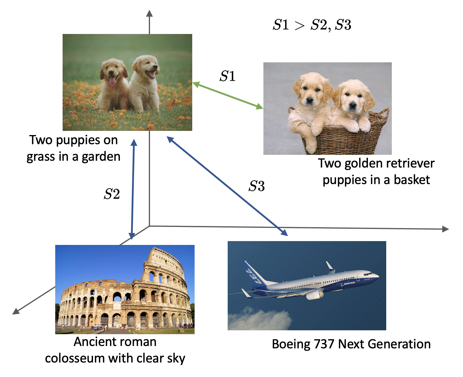
Figure 2: Hard Negative Margin Loss (HNML). Hard negative margin loss aims at keeping the hard negative examples closer to the positive than the normal negative samples.

The image-text contrastive loss $\ell_{CLIP}$, as illustrated in Section 3.1, aims at maximizing the distance between the positive pair and the corresponding negative one. While such an objective aligns the true image-text pairs, it poses no constraints on the overall geometry among data pairs [11]. After involving hard samples into the finetuning stage, equally maximizing the distance for normal negative pairs and hard negative pairs is an undesired way to utilize the information provided by hard negative samples. The intuition follows directly from Figure 2. In a desired representation space, the similarity between the positive sample and the hard negative sample, $S1$, should be greater than the similarity between the positive sample and normal negative samples, $S2,S3$. Therefore, to impose the additional geometric structure, we introduce the Hard Negative Margin Loss (HNML):

$$\ell_{margin}= \frac{1}{|B|}\sum_{j\in B}\max\big{(}0,sim(I_{i},T_{j})$$ (5)

$$-\min_{j^{\prime}\in\mathcal{H}^{p}_{i}}\{sim(I_{i},T_{j^{\prime}})\}\big{)},$$

where $\mathcal{H}^{p}_{i}$ is the hard negative samples for sample $z_{i}$, $|\mathcal{H}^{p}_{i}|=p,p\in\mathbb{R}^{+}$. Note, the HNML is memory efficient. No extra inner product computation is required. The geometric regularization is applied over the inner product matrix computed in the original CLIP loss (Equation  (1)).

Then, the well-trained model is finetuned with the following loss, where $\gamma$ is the hyperparameter balancing the two losses,

$$\ell_{finetune}=\ell_{CLIP}+\gamma\ell_{margin}.$$ (6)

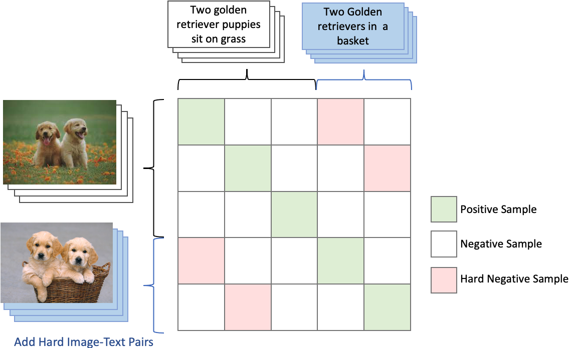
Figure 3: Finetuning CLIP with Hard Examples. For text-image pairs within a batch, we sample corresponding hard samples from the preprocess hard sample pool. By involving hard sample into the batch, the CLIP is fintuned with the text-image contrastive loss and the hard negative margin loss.

In all, to boost the performance of well-trained CLIP models without introducing extra data and extra parameters, we introduce the finetuning strategy which involve the hard samples prepared in the preprocessing stage into the batch composition of finetuning stage. As shown in Figure 3, for text-image pairs within the batch ${B}$, we randomly sample a subset ${B}^{\prime}$ as seeds. Then, for $z_{i}\in{B}^{\prime}$, we random select $p$ samples from $\mathcal{H}_{i}$ and denote the subset as $\mathcal{H}_{i}^{p}$. The actual training batch is $\overline{B}={B}\cup_{i=0}^{|{B}^{\prime}|}\mathcal{H}_{i}^{p}$. For the training pipeline, we summarize it the algorithm in Appendix A.2.

4 Experiments

Here we evaluate our approach across a broad range of vision and vision-language tasks.

4.1 Experimental setup

Training datasets. We mainly focus on finetuning well-trained models on Conceptual Captions 3M (CC3M) [31] and Conceptual Captions 12M (CC12M) [4], and a 15M subset of YFCC100M [32] collected by DECLIP  [20] CC3M and CC12M are relatively small but it has been used for benchmark evaluations in many works  [11, 20, 22] on language-image pretraining. with a different filtering strategy from Radford et al. [27]. It contains some additional data crawled from the Internet in addition to YFCC and is of higher quality than the subset in  [27]. We refer to it as YFCC15M.

Downstream datasets. We mainly verify the effectiveness of our methods through zero-shot image classification, linear probing of the visual representation learned by the visual encoder, and zero-shot image-text retrieval. For zero-shot classification, in addition to commonly used ImageNet  [7], CIFAR10, and CIFAR100 [17], we also verify the performance on 7 fine-grained classification datasets including Caltech101, Food101, Sun397, Flowers102, CUB, Stanford Cars and FGVC Aircraft. For the zero-shot image-text retrieval task, MS-COCO [21] and Flickr30K [25] are adopted.

Implementation Details. We conduct experiments on three different architectures, ResNet-50, ViT-B/32, and ViT-B/16, according to different datasets and pretrained models. Their details directly follow that of CLIP  [27]. When pretraining on CC3M and CC12M using CLIP model, we adopt ResNet-50 as the backbone. We use ViT-B/16 for SLIP model on CC3M and CC12M to match the setting in  [22]. While for pretraining on YFCC, we adopt ViT-B/32 in all experiments to fairly compare the results in  [20]. The input resolution of the image encoder is 224 $\times$ 224 and the maximum context length of the text encoder is 77. All of our experiments are conducted on 8 V100 GPUs with a batch size of 128 for ViT-B/16 models, and a batch size of 512 for ResNet-50 models and ViT-B/32 models. The dimension of the image and text embeddings is 1024 for ResNet-50 models and 512 for ViT-B/16 and ViT-B/32 models. We set $\gamma=1$ and $p=1$ for all the expriments by default. To save GPU memory, automatic mixed-precision is used. To avoid the model from overfitting to potential harmful distribution induced by the hard sample batch, we use early stopping if there’s no performance gain within 5 consecutive epochs.

In the preparation of hard samples, we employ the unsupervisedly pretrained vision transformer, DINO VITs8, as the image encoder [3]. As for the text encoder, we utilize the SentenceT [28] pretrained transformer, which is trained on a dataset comprising over 1 billion sentences gathered from the internet. The embedding sizes are 384 for DINO VITs8 and 768 for SentenceT. For the CC3M dataset, hard pair mining can be accomplished in 1 hour and 9 minutes using a single V100 GPU. In the case of the CC12M dataset, the complete hard pair mining process takes 9 hours and 11 minutes on 8 V100 GPUs. For the 6M and 3M approximated versions, hard pair mining requires 5 hours 3 minutes and 2 hours 18 minutes, respectively. Regarding the FYCC dataset, the full version can be processed in 17 hours and 41 minutes on 8 V100 GPUs, while the 6M and 3M approximated hard pair mining tasks take 6 hours 19 minutes and 3 hours 27 minutes, respectively.

4.2 Main results and discussion

4.2.1 Zero-shot classification

		ImageNet	CIFAR10	CIFAR100
CC3M	CYCLIP [11]	22.08	51.45	23.15
	CLOOB [9]	23.97	-	-
	CLIP [27]	19.04	33.06	13.77
	CLIP-Helip	19.86	34.05	14.13
	SLIP [22]	23.00	65.61	34.69
	SLIP-Helip	26.05	68.18	37.77
CC12M	CLIP [27]	30.27	51.07	21.94
	CLIP-Helip	32.05	52.27	24.51
	SLIP [22]	41.17	81.30	53.68
	SLIP-Helip	45.64	82.31	53.79
YFCC15M	SLIP [22]	25.29	60.19	26.80
	SLIP∗ [20]	34.30	-	-
	SLIP-Helip	35.43	75.49	47.84
	DECLIP [20]	36.05	78.12	50.60
	DECLIP∗[20]	43.20	-	-
	DECLIP-Helip	43.80	84.88	56.31

Table 1: Zero-shot Performance on ImageNet, CIFAR10 and CIFAR100. The leftmost column indicates the pretraining datasets. ^∗ is the number reported in [20].

Pretraining Dataset	Method	Caltech101	Food101	Sun397	Flowers102	CUB	Stanford Cars	FGVC Aircraft	Average
CC3M	CLIP	42.14	13.02	27.08	13.37	3.45	1.08	1.02	14.45
	CLIP-Helip	48.08	13.11	28.94	13.61	3.70	1.17	1.11	15.67
	SLIP	54.01	16.03	29.19	12.06	4.70	1.21	1.50	16.96
	SLIP-Helip	66.89	17.05	33.69	15.16	4.85	1.19	1.29	20.12
CC12M	CLIP	63.78	31.53	37.86	19.56	7.32	14.22	2.49	25.25
	CLIP-Helip	64.85	36.49	38.22	24.73	8.58	15.59	2.97	27.35
	SLIP	76.33	52.33	44.96	31.81	10.50	22.53	3.06	34.50
	SLIP-Helip	80.28	54.86	47.53	31.39	10.56	25.67	4.08	36.34

Table 2: Zero-shot Performance on Fine-grained Image Classification . On a variety of fine-grained image classification benchmarks, models finetuned by Helip achieves consistent performance gains compared to their original counterparts.

Pretraining Dataset	Method	Caltech101	Food101	Sun397	Flowers102	CUB	Stanford Cars	FGVC Aircraft	Average
CC3M	CYCLIP [11]	80.88	54.95	-	83.74	-	22.72	28.02	-
	CLIP [27]	80.11	53.82	56.40	84.07	40.30	22.70	35.61	53.29
	CLIP-HELIP	82.49	59.79	59.56	87.84	46.19	30.01	42.48	58.34
	SLIP [22]	87.96	72.50	66.96	91.91	49.77	39.25	45.87	64.89
	SLIP-Helip	89.64	73.09	67.67	93.02	53.16	42.44	48.66	66.81
CC12M	CLIP [27]	85.35	68.00	64.45	87.88	48.75	57.80	40.32	64.65
	CLIP-Helip	85.87	68.89	64.95	88.36	49.41	58.55	40.17	65.17
	SLIP [22]	92.89	83.63	74.34	94.87	60.99	73.43	52.23	76.05
	SLIP-Helip	92.85	84.25	74.74	95.09	60.53	74.23	52.36	76.29

Table 3: Linear Probe Performance on Fine-grained Image Classification. We report the linear probe performance on a variety of classification benchmarks. In average, both the CLIP and SLIP pretrained on CC3M and CC12M are improved.

We compare zero-shot performances of the CLIP, SLIP, DECLIP, and those models finetuned by Helip on CC3M, CC12M and YFCC15M. We denote the models finetuned by Helip as CLIP-Helip , SLIP-Helip , and DECLIP-Helip respectively. As shown in Table 1, models further finetuned by Helip consistently get significant improvements on the three datasets compared with their counterparts. Specifically, on CC3M, with the help of Helip , zero-shot classification accuracy on ImageNet of CLIP model was improved from 19.04% to 19.86%. While SLIP model has a performance boost of over 13%, compared with its original number, achieving 26.05% accuracy on ImageNet. We additionally include two baseline methods: CYCLIP [11] and CLOOB [9] for reference. As for pretraining on CC12M, we directly adopted the checkpoints released by SLIP [22]. SLIP-Helip outperforms its counterpart by 4.47% in zero-shot accuracy on ImageNet. Because the pretrained DECLIP doesn’t have open-sourced parameters for CC3M and CC12M, we only compare DECLIP and the DECLIP-Helip on YFCC15M. On YFCC15M, we report the performance of SLIP and DECLIP achieved with the evaluation pipeline implemented in the work [20] and denote them as SLIP^∗ and DECLIP^∗. We notice that both SLIP and DECLIP are boosted by Helip. On average, SLIP and DECLIP are improved by 15.49% and 6.74% correspondingly.

Intuitively, by involving image-text pairs that are not a match, but are difficult to differentiate from true positive pairs in contrastive learning, Helip has the potential to improve the discriminative power of visual embedding generated by CLIP model. The discriminative ability is beneficial to classification tasks, especially for the fine-grained classification dataset. Therefore, we also evaluate zero-shot classification on 7 fine-grained classification datasets in Table 2. As can be seen from the table SLIP-Helip boosts the zero-shot accuracy of SLIP on Caltech101 by 12.88% and 3.95% when pretraining on CC3M and CC12M respectively. Both CLIP and SLIP models witness consistent improvements with their Helip counterparts.

4.2.2 Linear probing

The linear probing task trains a randomly initialized linear classifier on the feature extracted from the frozen image encoder on the downstream dataset. To accomplish this, we train the logistic regression classifier using scikit-learn’s L-BFGS implementation [24], with maximum 1,000 iterations on those 7 datasets. For each dataset, we search for the best regularization strength factor on the validation set over 45 logarithmically spaced steps within the range 1e-6 to 1e+5.

Experimental results in Table 3 demonstrate that both CLIP-Helip and SLIP-Helip have consistent improvements over their counterparts on almost all 7 datasets. Note that on CC12M SLIP-Helip performs marginally better on 5 out of 7 datasets. It’s probably because the self-supervision of SLIP [22] within the visual modal can be beneficial for learning fine-grained visual embedding, while SLIP-Helip doesn’t include image self-supervision during the training. In addition, we did not match the training batch size as SLIP [22] because of resource limitations. A combination of Helip and image self-supervision and larger training batch size may be a potential direction for achieving better linear probe performance.

4.2.3 Zero-shot retrieval

Pretraining Dataset	Method	COCO		Flickr30K
		R@1 $\uparrow$	R@5 $\uparrow$	R@1 $\uparrow$	R@5 $\uparrow$
CC3M	CLIP	14.4	34.1	31.7	56.0
	CLIP-Helip	17.8	39.8	35.4	61.0
	SLIP	22.3	45.6	39.6	68.6
	SLIP-Helip	23.4	48.3	41.8	69.6
CC12M	CLIP	26.9	52.6	47.2	74.3
	CLIP-Helip	27.8	54.3	48.2	75.4
	SLIP	39.0	66.0	65.4	90.1
	SLIP-Helip	39.4	67.2	66.2	89.7

Table 4: Zero-shot image-text retrieval results on MSCOCO and Flickr. $\uparrow$ indicates higher is better. Combining with Helip, CLIP and SLIP show the best retrieval performance.

We evaluate Helip  on zero-shot image-to-text retrieval tasks on MS-COCO  [21] and Flickr30K  [25]. We compare CLIP, SLIP, and their counterparts trained on CC3M and CC12M respectively in Table 4. As shown in the table, both CLIP and SLIP benefit from Helip .

4.3 Comparison with different hard sample mining methods

We evaluate the efficacy of the proposed method in enhancing the discriminative capacity of learned representations by comparing its zero-shot classification performance with that of other hard sample mining strategies. As described in the Section 2, a common way to define hard pairs is through intra-modality similarity. Hence, we introduce the hard sample mining methods depending on image similarity and text similarity and denote them as IM and TM correspondingly. For a given target pair, we compute the cosine similarity between its image/text representation and those of the remaining dataset. The image and text representations are encoded using a pretrained Resnet50 and BERT, respectively. As a preprocessing step, both IM and TM methods mine hard negatives. Subsequently, we integrate the mined hard samples into the training pipeline of the CLIP+IM and CLIP+TM methods and optimize the original contrastive loss to finetune the model. Additionally, we employ the hard negative contrastive loss, HN-NCE, proposed by Radenovic et al. [26], as a baseline. HN-NCE up-samples the weight of hard-negatives identified by the current model. As shown in Table 5, when the CC3M pretrained CLIP model is combined with Helip, its performance significantly outperforms other techniques.

	Imagenet	CIFAR10	CIFAR100
CLIP + Helip	19.86	34.05	14.13
CLIP + TM	16.70	28.71	9.67
CLIP + IM	16.93	29.22	10.42
CLIP + HN-NCE	19.47	29.88	11.83

Table 5: Zero-shot Performance for CLIP with different hard sample mining methods on CC3M. Helip consistently outperform other local/global hard sample mining methods by a large margin.

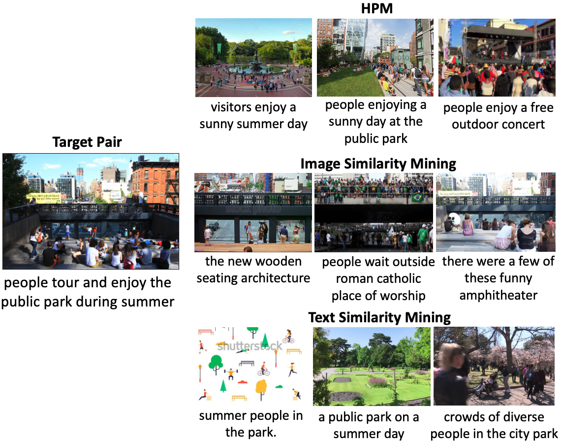
Figure 4: Hard samples selected by different methods. Compared to samples mined using the visual or textual modality, hard samples mined by HPM are more difficult.

We visualize the mined hard samples obtained from three different preprocessing methods, namely, hard pair mining (HPM), image similarity mining (IM), and text similarity mining (TM), in Figure 4. The image-text pairs selected by HPM are displayed in the first row, while the second and third rows show the pairs selected by IM and TM, respectively. We observe that the captions of the hard pairs mined with image similarity are only loosely connected with the image of the target pair. For samples mined by TM, their images are even mismatched with the caption of the target pair. The fact that pairs mined by TM is easier than IM is also reflected in the Table 5, where the zero-shot performance of the CLIP+IM method consistently outperforms the CLIP+TM method across three datasets.

4.4 Effect of hard negative margin loss

We investigate the impact of using hard negative margin loss (HNML) on the performance of the SLIP model. Specifically, we evaluate the SLIP model, which is pre-trained on the CC3M dataset, with and without finetuning using HNML. Our evaluation involves a comparison of the zero-shot classification performance of the model on ImageNet, CIFAR 100, and CIFAR 10 datasets. Our findings, which are presented in Table 6, indicate that the SLIP model performs better with HNML finetuning on ImageNet and CIFAR 100. However, without HNML, the model achieves better performance on CIFAR 10. This observation is possibly due to the HNML introducing additional discriminative power to the learned representations by utilizing the distance between classes as the cost. Consequently, for classification datasets with a larger number of sub-classes, such as ImageNet and CIFAR 100, the use of HNML during training can result in improved classification performance.

	ImageNet	CIFAR10	CIFAR100	Avg.
wo HNML	24.94	69.44	36.35	43.57
w HNML	26.05	68.18	37.77	44.00

Table 6: SLIP finetuned with and without hard negative margin loss. With hard negative samples mined by HPM, we report the zero-shot classification performance of CC3M pretrained SLIP model optimized with and without HNML.

4.5 Effect of hard pair mining approximation

To accelerate the hard pairs mining step of Helip, the approximated HPM is introduced. We compared the zero-shot performance of SLIP finetuned with hard samples mined by different methods and summarized the result in Table 7. For the all three settings, we keep the hyperparameter $k=500$ as the previous. Besides, we set subset $\widetilde{\mathcal{D}}_{i}$ with size 3M and 6M. Correspondingly, we denote the approximated Helip with 3M and 6M subset as Helip-3M and Helip-6M. As shown in Table 7, the zero-shot performance of Helip-3M and Helip-6M are competitive with the HPM mining hard sample globally. The result indicates that the approximated HPM is an efficient choice to mine hard samples and effective enough for contrastive learning. Besides, it indicates that approximated HPM has the potential to scale up to mine hard samples for much larger datasets for pre-training. We leave this as future work.

	Imagenet	CIFAR10	CIFAR100
Helip- 3M	45.07	82.42	55.22
Helip- 6M	44.98	81.64	56.62
Helip- Full	45.64	82.31	53.79

Table 7: Zero-shot Performance for SLIP + Helip on CC12M with hard samples mined with HPM and Approximated versions. Compared with hard samples mined with HPM, the approximated versions with constant base size are competitive with the full version.

Besides, we visualized the hard samples selected by those three methods. In Figure 5, the left image-text pair is the target one, and the pairs in the first row are picked by HPM. The second and third row show the image-text pairs mined by 6M approximated HPM and 3M approximated HPM. The visualization comparison show that the hard samples mined by the approximated HPM are also close enough to the target pair. We leave more visualization results in Appendix A.1.

Figure 5: HPM and approximated HPM. We show the hard samples mined by HPM and approximated HPM. The quality of hard samples mined by approximated HPM is competitive with the samples mined by HPM.

5 Conclusion and Future Work

In conclusion, our experiments demonstrate that incorporating hard negative samples and a simple objective change can consistently and substantially improve the performance of language-image contrastive models through finetuning. Our proposed approach, Helip , can be applied generically to any large-scale dataset and well-trained models for improved performance with smaller training schedules. The Hard Pair Mining (HPM) component efficiently mines qualified hard pairs, while the Hard Negative Margin Loss (HNML) effectively utilizes the supervision information provided by hard negative pairs. Our experiments show that the Helip framework can boost pretrained VLMs on zero-shot classification and retrieval benchmarks, as well as downstream linear probe tasks.

Moving forward, several avenues for future research present themselves. First, we aim to explore composition-aware fine-tuning for VLMs, which could potentially enable more effective utilization of multimodal information. Moreover, we are intrigued by the prospect of combining parameter-efficient tuning [12] with Helip  potentially further enhancing performance. Another area of interest is scaling up the dataset size and examining the applicability of the scaling law to our method. We also intend to investigate how the integration of our boosting algorithm might alter the multimodal dataset curation algorithm [10]. Ultimately, we hope our work will serve as a catalyst for additional research in the fine-tuning of pre-trained, large-scale multimodal models.

Appendix A Appendix

A.1 More visualization results

We provide more visualization results about the hard samples mined by different methods. As shown in the Figure 6, the hard samples mined by HPM are more similar to the target one (the left top). Besides, we found that, for samples with less objectives, the image and text mining method is able to deliver reasonable hard counterpart, such as the case “the harbor a small village”. However, for the complex scene, only the HPM is able to provide samples challenging enough, such as the case “people tour and enjoy the public park during summer”. The web-crawled dataset include a large amount of complex cases. We think that is why training with the hard samples mined by HPM can achieve a better result.

We provide additional visualization results for the hard samples mined using various techniques. The hard samples mined by HPM are more comparable to the target one, as illustrated in the Figure 6 (the left top). Besides, we found that the image- and text-mode mining method can give a relatively reasonable hard counterpart for samples with less objectives, such as the case “the harbor a little settlement.”. But, only the HPM is able to deliever samples that are difficult enough for the complicated scene, such as the case “people tour and enjoy the public park throughout summer.”. The dataset gathered from the web contains a large number of complex cases. We believe this is the reason training on the hard samples extracted by HPM can produce superior results.

A.2 Algorithm

We summrize the hard pair mining and the training pipeline of Helip in Algorithm 1 and  2 respectively.

Algorithm 1 Hard Pair Mining (HPM).

Pretrained unimodal vision model: $f_{text}$

Pretrained unimodal vision model: $f_{image}$

Dataset $\mathcal{D}=\{(x_{1}^{I},x_{1}^{T}),(x_{1}^{I},x_{1}^{T}),\cdots,(x_{N}^{I},x_{N}^{T})\}$

Hard pairs number $k$

for $i\in[1,N]$ do

     $s\leftarrow[0,0,\cdots,0]^{\top}\in\mathbb{R}^{N}$

     $I_{i}\leftarrow f_{image}(x_{i}^{I})$ and $T_{i}\leftarrow f_{text}(x_{i}^{T})$

     for $j\in[1,N]$ do

         $I_{j}\leftarrow f_{image}(x_{j}^{I})$ and $T_{j}\leftarrow f_{text}(x_{j}^{T})$

         $s_{j}\leftarrow\frac{I_{i}\cdot I_{j}}{\left\|I_{i}\right\|_{2}\cdot\left\|I_{j}\right\|_{2}}\cdot\frac{T_{i}\cdot T_{j}}{\left\|T_{i}\right\|_{2}\cdot\left\|T_{j}\right\|_{2}}$

     end for

     $\mathcal{H}_{i}\leftarrow Argmax(s,k)$

end for

Note, the inner for loop, shown in Algorithm 1, will be repeatedly computed. To accelerate the hard pair mining and avoid unnecessary computational overhead, we compute the inner for loop firstly and save the encoded image features and text features. Besides, the outer loop is parallelized in the implementation.

Algorithm 2 Hard samplE for boosting contrastive Language-Image Pretrained models (Helip) .

Hard Pair Mining algorithm, $HPM()$

Pretrained unimodal vision model: $f_{text}$

Pretrained unimodal vision model: $f_{image}$

Dataset $\mathcal{D}=\{(x_{1}^{I},x_{1}^{T}),(x_{1}^{I},x_{1}^{T}),\cdots,(x_{N}^{I},x_{N}^{T})\}$

Pretrained contrastive language-image model $\{\phi_{image},\phi_{text}\}$

Hard pairs number $k$

Hard negative margin strength $\gamma$

Sampled hard negatives number $p$

Learning ratio $\eta$

Batch size $b$

Training iteration number $E$

$\mathcal{H}\leftarrow HPM(\mathcal{D},f_{text},f_{image},k)$

for $iter\in[1,E]$ do

     $B\leftarrow\{z_{1},\ldots,z_{b}\}\stackrel{{\scriptstyle\text{ i.i.d. }}}{{\sim}}Uniform(\mathcal{D})$

     for $z_{i}\in B$ do

         $\mathcal{H}_{i}^{p}\leftarrow\{z_{i},\ldots,z_{p}\}\stackrel{{\scriptstyle\text{ i.i.d. }}}{{\sim}}Uniform(\mathcal{H}_{i})$

         $\overline{B}\leftarrow B\cup\mathcal{H}_{i}^{p}$

     end for

     $\text{Compute loss}~{}\ell_{finetune}\text{, Equation (6), with samples}~{}\overline{B}$

     $\phi_{image}\leftarrow\phi_{image}+\eta\cdot\partial_{\phi_{image}}\ell_{finetune}$

     $\phi_{text}\leftarrow\phi_{text}+\eta\cdot\partial_{\phi_{text}}\ell_{finetune}$

end for

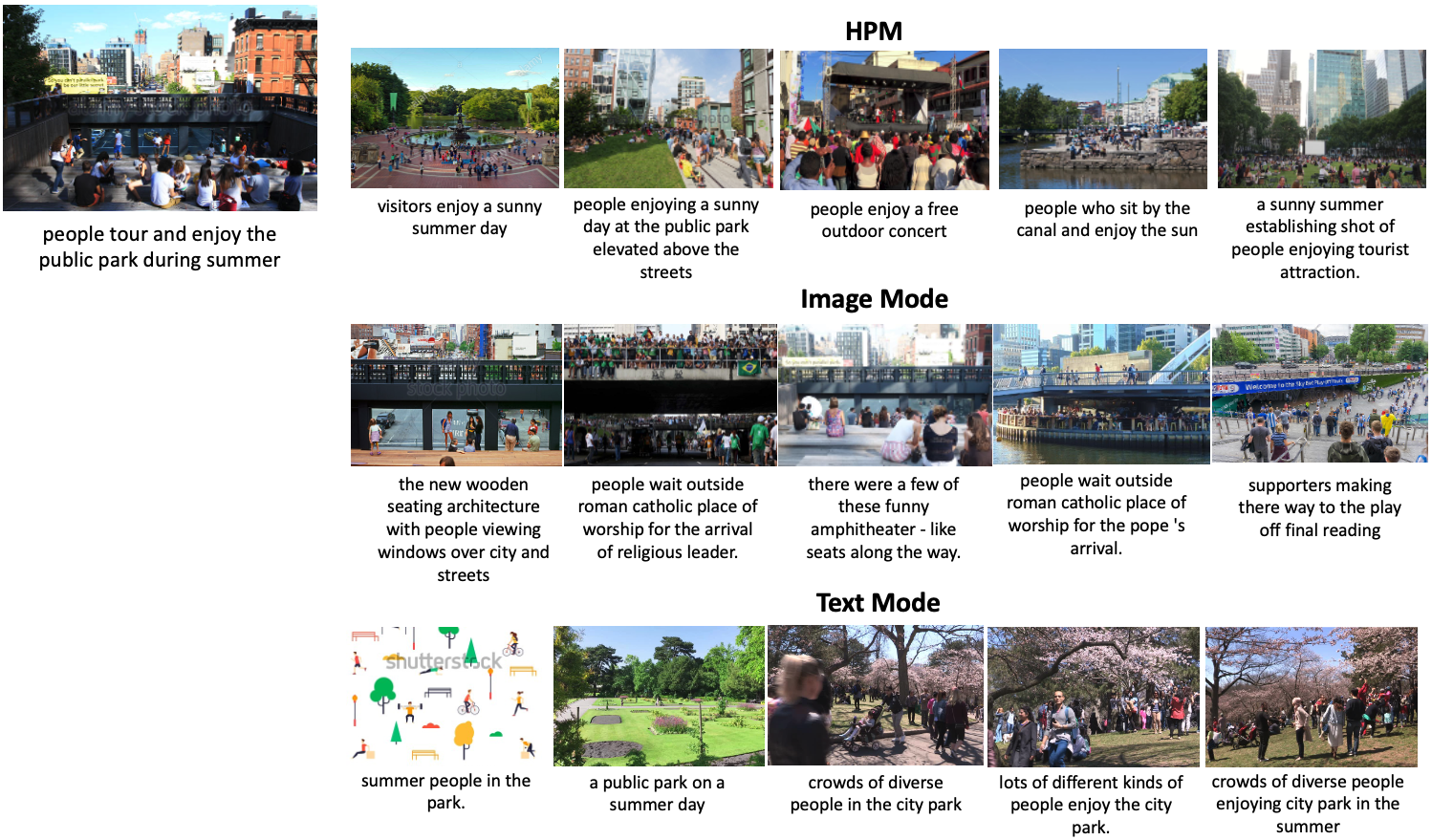
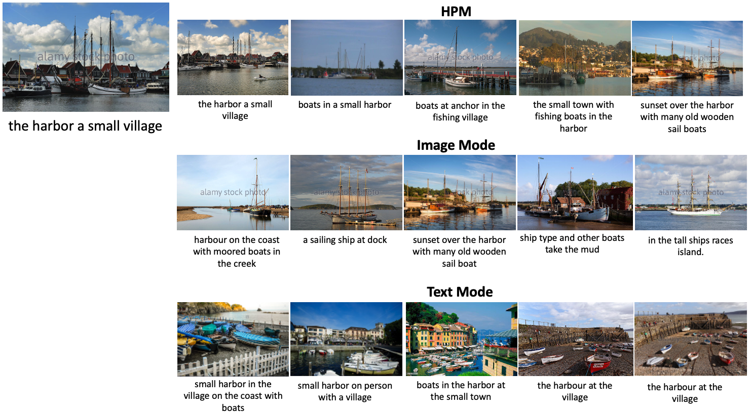
Figure 6: Hard samples selected by different methods.

References

- [1] Alberto Baldrati, Marco Bertini, Tiberio Uricchio, and Alberto Del Bimbo. Conditioned and composed image retrieval combining and partially fine-tuning clip-based features. In Proc. of CVPR, 2022.
- [2] Tiffany Tianhui Cai, Jonathan Frankle, David J. Schwab, and Ari S. Morcos. Are all negatives created equal in contrastive instance discrimination? ArXiv preprint, 2020.
- [3] Mathilde Caron, Hugo Touvron, Ishan Misra, Hervé Jégou, Julien Mairal, Piotr Bojanowski, and Armand Joulin. Emerging properties in self-supervised vision transformers. In Proc. of ICCV, 2021.
- [4] Soravit Changpinyo, Piyush Sharma, Nan Ding, and Radu Soricut. Conceptual 12m: Pushing web-scale image-text pre-training to recognize long-tail visual concepts. In Proc. of CVPR, 2021.
- [5] Ting Chen, Simon Kornblith, Mohammad Norouzi, and Geoffrey E. Hinton. A simple framework for contrastive learning of visual representations. In Proc. of ICML, 2020.
- [6] Xinlei Chen, Haoqi Fan, Ross B. Girshick, and Kaiming He. Improved baselines with momentum contrastive learning. ArXiv preprint, 2020.
- [7] Jia Deng, Wei Dong, Richard Socher, Li-Jia Li, Kai Li, and Fei-Fei Li. Imagenet: A large-scale hierarchical image database. In Proc. of CVPR, 2009.
- [8] Jacob Devlin, Ming-Wei Chang, Kenton Lee, and Kristina Toutanova. BERT: Pre-training of deep bidirectional transformers for language understanding. In Proc. of NAACL, 2019.
- [9] Andreas Fürst, Elisabeth Rumetshofer, Viet Tran, Hubert Ramsauer, Fei Tang, Johannes Lehner, David P. Kreil, Michael Kopp, Günter Klambauer, Angela Bitto-Nemling, and Sepp Hochreiter. CLOOB: modern hopfield networks with infoloob outperform CLIP. ArXiv preprint, 2021.
- [10] Samir Yitzhak Gadre, Gabriel Ilharco, Alex Fang, Jonathan Hayase, Georgios Smyrnis, Thao Nguyen, Ryan Marten, Mitchell Wortsman, Dhruba Ghosh, Jieyu Zhang, et al. Datacomp: In search of the next generation of multimodal datasets. ArXiv preprint, 2023.
- [11] Shashank Goel, Hritik Bansal, Sumit Bhatia, Ryan A Rossi, Vishwa Vinay, and Aditya Grover. Cyclip: Cyclic contrastive language-image pretraining. ArXiv preprint, 2022.
- [12] Junxian He, Chunting Zhou, Xuezhe Ma, Taylor Berg-Kirkpatrick, and Graham Neubig. Towards a unified view of parameter-efficient transfer learning. In Proc. of ICLR, 2022.
- [13] Kaiming He, Xiangyu Zhang, Shaoqing Ren, and Jian Sun. Deep residual learning for image recognition. In Proc. of CVPR, 2016.
- [14] Tri Huynh, Simon Kornblith, Matthew R. Walter, Michael Maire, and Maryam Khademi. Boosting contrastive self-supervised learning with false negative cancellation. In IEEE/CVF Winter Conference on Applications of Computer Vision, WACV 2022, Waikoloa, HI, USA, January 3-8, 2022, 2022.
- [15] Chao Jia, Yinfei Yang, Ye Xia, Yi-Ting Chen, Zarana Parekh, Hieu Pham, Quoc V. Le, Yun-Hsuan Sung, Zhen Li, and Tom Duerig. Scaling up visual and vision-language representation learning with noisy text supervision. In Proc. of ICML, 2021.
- [16] Yannis Kalantidis, Mert Bülent Sariyildiz, Noé Pion, Philippe Weinzaepfel, and Diane Larlus. Hard negative mixing for contrastive learning. In Proc. of NeurIPS, 2020.
- [17] Alex Krizhevsky, Geoffrey Hinton, et al. Learning multiple layers of features from tiny images. 2009.
- [18] Junnan Li, Dongxu Li, Caiming Xiong, and Steven C. H. Hoi. BLIP: bootstrapping language-image pre-training for unified vision-language understanding and generation. In Proc. of ICML, 2022.
- [19] Junnan Li, Ramprasaath R. Selvaraju, Akhilesh Gotmare, Shafiq R. Joty, Caiming Xiong, and Steven Chu-Hong Hoi. Align before fuse: Vision and language representation learning with momentum distillation. In Proc. of NeurIPS, 2021.
- [20] Yangguang Li, Feng Liang, Lichen Zhao, Yufeng Cui, Wanli Ouyang, Jing Shao, Fengwei Yu, and Junjie Yan. Supervision exists everywhere: A data efficient contrastive language-image pre-training paradigm. In Proc. of ICLR, 2022.
- [21] Tsung-Yi Lin, Michael Maire, Serge J. Belongie, James Hays, Pietro Perona, Deva Ramanan, Piotr Dollár, and C. Lawrence Zitnick. Microsoft COCO: common objects in context. In Proc. of ECCV, 2014.
- [22] Norman Mu, Alexander Kirillov, David A. Wagner, and Saining Xie. SLIP: self-supervision meets language-image pre-training. In Proc. of ECCV, 2022.
- [23] Antonio Norelli, Marco Fumero, Valentino Maiorca, Luca Moschella, Emanuele Rodolà, and Francesco Locatello. Asif: Coupled data turns unimodal models to multimodal without training. ArXiv preprint, 2022.
- [24] Fabian Pedregosa, Gaël Varoquaux, Alexandre Gramfort, Vincent Michel, Bertrand Thirion, Olivier Grisel, Mathieu Blondel, Peter Prettenhofer, Ron Weiss, Vincent Dubourg, et al. Scikit-learn: Machine learning in python. the Journal of machine Learning research, 2011.
- [25] Bryan A. Plummer, Liwei Wang, Chris M. Cervantes, Juan C. Caicedo, Julia Hockenmaier, and Svetlana Lazebnik. Flickr30k entities: Collecting region-to-phrase correspondences for richer image-to-sentence models. In Proc. of ICCV, 2015.
- [26] Filip Radenovic, Abhimanyu Dubey, Abhishek Kadian, Todor Mihaylov, Simon Vandenhende, Yash Patel, Yi Wen, Vignesh Ramanathan, and Dhruv Mahajan. Filtering, distillation, and hard negatives for vision-language pre-training. CoRR, 2023.
- [27] Alec Radford, Jong Wook Kim, Chris Hallacy, Aditya Ramesh, Gabriel Goh, Sandhini Agarwal, Girish Sastry, Amanda Askell, Pamela Mishkin, Jack Clark, Gretchen Krueger, and Ilya Sutskever. Learning transferable visual models from natural language supervision. In Proc. of ICML, 2021.
- [28] Nils Reimers and Iryna Gurevych. Sentence-BERT: Sentence embeddings using Siamese BERT-networks. In Proc. of EMNLP, 2019.
- [29] Joshua David Robinson, Ching-Yao Chuang, Suvrit Sra, and Stefanie Jegelka. Contrastive learning with hard negative samples. In Proc. of ICLR, 2021.
- [30] Anshul Shah, Suvrit Sra, Rama Chellappa, and Anoop Cherian. Max-margin contrastive learning. In Proc. of AAAI, 2022.
- [31] Piyush Sharma, Nan Ding, Sebastian Goodman, and Radu Soricut. Conceptual captions: A cleaned, hypernymed, image alt-text dataset for automatic image captioning. In Proc. of ACL, 2018.
- [32] Bart Thomee, David A Shamma, Gerald Friedland, Benjamin Elizalde, Karl Ni, Douglas Poland, Damian Borth, and Li-Jia Li. Yfcc100m: The new data in multimedia research. Communications of the ACM, 2016.
- [33] Tongzhou Wang and Phillip Isola. Understanding contrastive representation learning through alignment and uniformity on the hypersphere. In Proc. of ICML, 2020.
- [34] Bichen Wu, Ruizhe Cheng, Peizhao Zhang, Tianren Gao, Joseph E. Gonzalez, and Peter Vajda. Data efficient language-supervised zero-shot recognition with optimal transport distillation. In Proc. of ICLR, 2022.
- [35] Lewei Yao, Runhui Huang, Lu Hou, Guansong Lu, Minzhe Niu, Hang Xu, Xiaodan Liang, Zhenguo Li, Xin Jiang, and Chunjing Xu. FILIP: fine-grained interactive language-image pre-training. In Proc. of ICLR, 2022.
- [36] Hongyi Zhang, Moustapha Cissé, Yann N. Dauphin, and David Lopez-Paz. mixup: Beyond empirical risk minimization. In Proc. of ICLR, 2018.