Self-similar algebraic spiral solution of 2-D incompressible Euler equations

Abstract.

In this paper, we prove the existence of self-similar algebraic spiral solutions of 2-D incompressible Euler equations for the initial vorticity of the form $|y|^{-\frac{1}{\mu}}\ \mathring{\omega}(\theta)$ with $\mu>\frac{1}{2}$ and $\mathring{\omega}\in L^{1}(\mathbb{T})$ satisfying $m$-fold symmetry ($m\geq 2$) and a dominant condition. As an important application, we prove the existence of weak solution when $\mathring{\omega}$ is a Radon measure on $\mathbb{T}$ with $m$-fold symmetry, which is related to the vortex sheet solution.

1. Introduction

In this paper, we study the 2-D incompressible Euler equations in $\mathbb{R}^{2}\times[0,+\infty)$:

(1.1) $$\begin{cases}\mathbf{v}_{t}+\mathbf{v}\cdot\nabla_{y}\mathbf{v}+\nabla P=0,\\ \text{ div }\mathbf{v}=0,\end{cases}$$

where $\mathbf{v}$ is the velocity and $P$ is the pressure. The vorticity-stream formulation of (1.1) takes as follows

(1.2) $$\begin{cases}\bm{\omega}_{t}+\mathbf{v}\cdot\nabla_{y}\bm{\omega}=0,\\ \mathbf{v}=\nabla^{\perp}_{y}\Psi,\quad\Delta_{y}\Psi=\bm{\omega},\end{cases}$$

where $\bm{\omega}$ is the vorticity, $\Psi$ is the stream function and $\nabla^{\perp}_{y}=(-\partial_{y_{2}},\partial_{y_{1}})$.

For smooth data, the 2-D Euler equations are globally well-posed due to $\|\bm{\omega}(t)\|_{L^{\infty}}\leq\|\bm{\omega}_{0}\|_{L^{\infty}}$. Let us refer to [8, 26, 25] for some classical results about the well-posedness and stability of steady solutions and recent breakthrough [5] on the ill-posedness in the borderline spaces. However, the long-time behavior of the solution is a long-standing problem. Let us refer to [30, 4, 24, 3, 20, 33] and references therein for some relevant results.

For non-smooth data, a classical result due to Yudovich [34] is the global existence and uniqueness of weak solution when the initial vorticity lies in $L^{\infty}(\mathbb{R}^{2})\cap L^{1}(\mathbb{R}^{2})$, which is related to the vortex patch solution. In fact, the global existence of weak solution also holds for the initial vorticity in $L^{p}(\mathbb{R}^{2})\cap L^{1}(\mathbb{R}^{2}),1\leq p<+\infty$. However, in the latter case, the uniqueness of weak solution remains open, see [6, 32] for recent progress. Another classical result due to Delort [11] is the global existence of weak solution when the initial vorticity is a Radon measure with distinguished sign. The qualitative behavior of Delort’s solution remains an important question. Let us refer to [13, 14] for recent important progress on singular vortex patch solutions.

In a series of remarkable works [15, 16, 17], Elling constructed a class of self-similar algebraic spiral solutions for 2-D Euler equations. The algebraic spiral solutions are important in applications since they are ubiquitous in physics [31]. Elling considered a class of locally integrable self-similar initial data of the form

(1.3) $$\bm{\omega}(y,t)\xrightarrow{t\to 0+}|y|^{-\frac{1}{\mu}}\ \mathring{\omega}(\theta),\qquad\theta=\measuredangle y\in\mathbb{T}:=\mathbb{R}/(2\pi\mathbb{Z}).$$

The main result in [16] is stated as follows.

Theorem 1.1.

Given $\varepsilon>0$ and $\mu>\frac{2}{3}$, there exists an $N_{0}\in\mathbb{N}$ so that a weak solution of (1.1) and (1.3) exists for all initial data $\mathring{\omega}$ satisfying the following conditions:

• Periodicity: $\mathring{\omega}$ is $\frac{2\pi}{N}$-periodic for $N\geq N_{0}$;

• Dominant rotation: the Fourier coefficients satisfy

  $$|\widehat{\mathring{\omega}}(0)|\geq\varepsilon\sum_{n\neq 0}|\widehat{\mathring{\omega}}(n)|.$$

The goal of this paper is to extend Elling’s remarkable result in three important aspects:

• In Theorem 1.1, $\mathring{\omega}$ lies in a Weiner algebra. We would like to allow $\mathring{\omega}\in L^{1}(\mathbb{T})$ and even $\mathring{\omega}\in\mathcal{M}(\mathbb{T})$ Radon measure. This kind of data is crucial for the construction of self-similar vortex sheet solution. This may be relevant to the non-uniqueness problem of weak solution of 2-D Euler equations with the initial vorticity in $L^{p}(\mathbb{R}^{2}),p<+\infty$.

• In Theorem 1.1, $N_{0}$ is a large positive integer. We would like to improve $N_{0}$.

• Extend the range of $\mu$ to $\mu>\frac{1}{2}$, which is a natural condition ensuring $\bm{\omega}_{0}\in L^{1}_{\text{loc}}(\mathbb{R}^{2})$.

To state our results, let us first introduce the definition of weak solution.

Definition 1.1.

A vector field $\mathbf{v}(y,t)$ is called a weak solution of the 2-D Euler equations (1.1) provided that

1. $\mathbf{v}\in C([0,\infty);L^{2}_{\text{loc}}(\mathbb{R}^{2};\mathbb{R}^{2}))$, i.e., for any $R>0$ we have $\mathbf{v}\in C([0,\infty);L^{2}(B_{R};\mathbb{R}^{2}))$, where $B_{R}=\{y\in\mathbb{R}^{2}:|y|\leq R\}$;

2. $\text{ div}_{y}\mathbf{v}=0$ in the sense of distributions, i.e.,

   $$\int_{\mathbb{R}^{2}}\nabla_{y}\eta(y,t)\cdot\mathbf{v}(y,t)\,dy=0,\qquad\forall t\geq 0,\ \forall\eta\in C_{c}^{\infty}\left(\mathbb{R}^{2}\times[0,\infty)\right);$$

3. $\mathbf{v}$ solves the 2-D Euler equations (1.1) in the sense of distributions, i.e., for any vector-field $\mathbf{w}\in C_{c}^{\infty}\left(\mathbb{R}^{2}\times[0,\infty);\mathbb{R}^{2}\right)$ with $\text{ div}_{y}\mathbf{w}=0$ there holds

   $$\int_{\mathbb{R}^{2}}\mathbf{v}\cdot\mathbf{w}\,dy\Big{|}_{t=0}+\int_{0}^{\infty}\int_{\mathbb{R}^{2}}\mathbf{v}\cdot\partial_{t}\mathbf{w}+\left(\mathbf{v}\otimes\mathbf{v}\right):\nabla_{y}\mathbf{w}\,dy\,dt=0,$$

   where $\mathbf{v}\otimes\mathbf{v}=\left(\mathbf{v}^{i}\mathbf{v}^{j}\right)$, $\nabla_{y}\mathbf{w}=\left(\frac{\partial\mathbf{w}^{j}}{\partial y_{i}}\right)$ and $A:B=\sum_{i,j=1}^{2}A_{ij}B_{ij}$.

For $\Omega\in L^{1}(\mathbb{T})$, we denote

$$P_{0}\Omega:=\frac{1}{2\pi}\int_{\mathbb{T}}\Omega(\theta)\,d\theta,\qquad P_{\neq}\Omega(\theta):=\Omega(\theta)-P_{0}\Omega\in L^{1}(\mathbb{T}).$$

Now our main result is stated as follows.

Theorem 1.2.

Let $\mu>\frac{1}{2}$ and $m\in\mathbb{N}_{+}\setminus\{1\}$. There exists $\varepsilon>0$, which is independent of $m\geq 2$, such that for any $\frac{2\pi}{m}-$periodic $\mathring{\omega}\in L^{1}(\mathbb{T})$ with the dominant condition

(1.4) $$\left\|P_{\neq}\mathring{\omega}\right\|_{L^{1}(\mathbb{T})}\leq\varepsilon m^{\frac{1}{2}}|P_{0}\mathring{\omega}|,$$

a weak solution $\mathbf{v}$ of (1.1) with the initial data (1.3) exists. Moreover, the vorticity $\bm{\omega}\in C([0,\infty);L^{1}_{\text{loc}}(\mathbb{R}^{2}))$.

Remark 1.3.

The velocity $\mathbf{v}$ is strongly continuous at $t=0$. Given the initial vorticity $\bm{\omega}_{0}(y)=|y|^{-\frac{1}{\mu}}\mathring{\omega}(\theta)$, the initial velocity can be recovered by $\mathbf{v}_{0}=\nabla_{y}^{\perp}\Psi_{0}$, with $\Psi_{0}(y)=|y|^{2-\frac{1}{\mu}}B(\theta)$, where $B$ is the only $\frac{2\pi}{m}$-periodic function satisfying $\gamma^{2}B+B^{\prime\prime}=\mathring{\omega}$, $\gamma=2-\frac{1}{\mu}$. See Proposition 7.3 for the details.

Let us give more remarks about our result.

• It seems possible to extend our result to the case when $m\geq 1$. This will be conducted in a future work.

• The stability of self-similar type solution constructed in Theorem 1.2 is a very interesting question. This may be relevant to the non-uniqueness problem of weak solution when the initial vorticity lies in $L^{p}(\mathbb{R}^{2}),p<+\infty$, see [6, 21, 32, 1] for relevant results.

• Another very interesting problem is to study the inviscid limit problem for the data considered in Theorem 1.2. We conjecture that our solution could be obtained via the vanishing viscosity limit. Thus, it is a physical solution in the sense of [2].

• Let us mention a recent important result [19] about self-similar spirals for the generalized surface quasi-geostrophic equations:

  $$\begin{cases}\theta_{t}+\mathbf{v}\cdot\nabla\theta=0,\\ \mathbf{v}=-\nabla^{\perp}(-\Delta)^{-1+\frac{\gamma}{2}}\theta.\end{cases}$$

  The case $\gamma=0$ corresponds to the 2-D Euler equations and $\gamma=1$ to the surface quasi-geostrophic equation. For $\gamma\in(0,1)$ and the initial data $\theta_{0}=r^{-(1+\alpha-\gamma)}\Omega(\theta)$ with $\alpha\in(1,1+\gamma)$ and $\Omega\in B_{L^{p}(\mathbb{T})}(1,\varepsilon),p>\frac{1}{1-\gamma},\varepsilon$ small, they constructed a self-similar solution of the form

  $$\theta(t,x)=\frac{1}{t^{(1+\alpha-\gamma)/(1+\alpha)}}\Theta\Big{(}\frac{x}{t^{1/(1+\alpha)}}\Big{)}.$$

  Our result deals with the important case $\gamma=0$ for $\Omega(\theta)\in L^{1}(\mathbb{T})$.

As an important application, we prove the existence of weak solution of 2-D Euler equations when the initial vorticity is a measure, which is related to the vortex sheet solution. We denote by $\mathcal{M}(\mathbb{T})$ the set of signed Radon measures on $\mathbb{T}$. Given a measure $\nu\in\mathcal{M}(\mathbb{T})$, we say that $\nu$ is $m$-fold symmetric if

$$\int_{\mathbb{T}}\eta\left(\theta+\frac{2\pi}{m}\right)\,d\nu(\theta)=\int_{\mathbb{T}}\eta(\theta)\,d\nu(\theta)\qquad\text{ for all }\eta\in C(\mathbb{T}).$$

For $\nu\in\mathcal{M}(\mathbb{T})$, we denote

$$P_{0}\nu:=\frac{1}{2\pi}\nu(\mathbb{T})\in\mathbb{R},\qquad P_{\neq}\nu:=\nu-P_{0}\nu\in\mathcal{M}(\mathbb{T}),$$

and $\|\nu\|$ the total variance measure of $\nu$.

Corollary 1.4.

Let $\mu>\frac{1}{2}$ and $m\in\mathbb{N}_{+}\setminus\{1\}$. There exists $\varepsilon>0$, which is independent of $m\geq 2$, such that for any $m$-fold symmetric $\mathring{\omega}\in\mathcal{M}(\mathbb{T})$ with the dominant condition

(1.5) $$\left\|P_{\neq}\mathring{\omega}\right\|\leq\varepsilon m^{\frac{1}{2}}|P_{0}\mathring{\omega}|,$$

a weak solution $\mathbf{v}$ of (1.1) with initial data (1.3) exists. Moreover, the vorticity $\bm{\omega}\in C([0,\infty);\mathcal{D}^{\prime}(\mathbb{R}^{2}))$.

Remark 1.5.

The qualitative behavior of Delort’s solution remains an important question. In a forthcoming work, we will explore the qualitative behavior of weak solution constructed in Corollary 1.4, which is a key step toward the long-standing problem: Existence of self-similar algebraic spiral vortex sheet solution, see [28, 29] for numerical results. Let us refer to [9, 10] for recent developments on the logarithmic spiral vortex sheet solution.

2. Sketch of the proof

The 2-D incompressible Euler equations (1.2) can be reformulated as follows: find two scalar functions $\bm{\omega},\Psi$ defined for $(y,t)\in\mathbb{R}^{2}\times(0,\infty)$, such that

(2.1) $$\begin{cases}\bm{\omega}_{t}+\nabla_{y}^{\perp}\Psi\cdot\nabla_{y}\bm{\omega}=0,\\ \Delta_{y}\Psi=\bm{\omega}.\end{cases}$$

We seek solutions of $\eqref{2dEuler-vorticity}$ which are (algebraically) self-similar: with $x=t^{-\mu}y$,

(2.2) $$\mathbf{v}(y,t)=t^{\mu-1}v(x),\qquad\bm{\omega}(y,t)=t^{-1}\omega(x),\qquad\Psi(y,t)=t^{2\mu-1}\psi(x)$$

for some exponent $\mu>0$. Inserting (2.2) into (2.1) yields the equations

(2.3) $$\begin{cases}\left(\nabla_{x}^{\perp}\psi-\mu x\right)\cdot\nabla_{x}\omega=\omega,\\ \Delta_{x}\psi=\omega.\end{cases}$$

To study spirals converging to a common origin, it is convenient to use polar coordinates:

$$\mathbf{a}=(r,\theta),\qquad r=|x|,\qquad\theta=\measuredangle x=\measuredangle y\in\mathbb{T}:=\mathbb{R}/(2\pi\mathbb{Z}),$$

where $\measuredangle$ is the counterclockwise angle from the positive horizontal axis. Then we have

$$\begin{cases}\frac{1}{r}\left(\psi_{r}\omega_{\theta}-\psi_{\theta}\omega_{r}\right)-\mu r\omega_{r}=\omega,\\ \psi_{rr}+\frac{1}{r}\psi_{r}+\frac{1}{r^{2}}\psi_{\theta\theta}=\omega.\end{cases}$$

Note that the second equation in the above system is indeed a Poisson equation in the coordinates $(\log r,\theta)$.

In Section 3, we introduce the adapted coordinates $(\beta,\phi)\in\mathbb{R}_{+}\times\mathbb{T}$ with the relationship

$$\theta=\beta+\phi,\qquad\psi_{\beta}=-\mu|x|^{2}=-\mu r^{2}.$$

Under this new coordinates, the system can be transformed into

$$\mathcal{F}(\psi,\Omega):=\partial_{\varphi}\left(\frac{2\psi_{\beta}\psi_{\varphi}}{\psi_{\beta\varphi}}-\frac{\psi_{\beta\phi}}{\psi_{\beta\varphi}}\cdot\frac{\psi_{\beta\varphi}\psi_{\phi}-\psi_{\beta\phi}\psi_{\varphi}}{2\psi_{\beta}}\right)+\partial_{\phi}\left(\frac{\psi_{\beta\varphi}\psi_{\phi}-\psi_{\beta\phi}\psi_{\varphi}}{2\psi_{\beta}}\right)+\frac{\psi_{\beta\varphi}\psi_{\varphi}^{-\frac{1}{2\mu}}}{2\mu}\Omega=0,$$

where $\partial_{\varphi}:=\partial_{\phi}-\partial_{\beta}$. This nonlinear equation has a special solution:

$$\psi_{0}=\frac{1}{2\mu-1}\beta^{1-2\mu},\qquad\Omega_{0}=2-\mu^{-1}=:\gamma.$$

Since the solution we find is singular in $\beta$, motivated by [14], we introduce the weighted Hölder type spaces. The choices of the functional spaces for the $m$-fold symmetric solution like $\psi\in Y_{m},\Omega\in\mathcal{W}_{m}$ and $\mathcal{F}\in Z_{m}$ are quite subtle and are closely related to the properties of the solutions. Let us emphasize that our functional spaces have Banach algebraic properties, which will simplify the proof of $C^{2}$ regularity of the nonlinear map $\mathcal{F}$ to a great extent. See Section 4 for the definitions of various functional spaces.

We will apply the implicit function theorem to solve the nonlinear equation $\mathcal{F}(\psi,\Omega)=0$ for $\Omega$ near $\Omega_{0}=\gamma$. The first step is to prove that nonlinear map $\mathcal{F}:Y_{m}\times\mathcal{W}_{m}\to Z_{m}$ is a $C^{2}$ map in a neighborhood of $(\psi_{0},\Omega_{0})$, which will be conducted in Section 5. We remark that for the application of the implicit function theorem, it is enough to prove $C^{1}$ regularity of nonlinear map; however, here we need $C^{2}$ regularity, because we want to show that the small neighborhood given by the implicit function theorem is independent of $m$, although the functional spaces rely on $m$. The second step is to prove the solvability of the linearized problem around special solution $(\psi_{0},\Omega_{0})$:

$$\mathcal{L}(\psi)=\frac{1}{\mu}\partial_{\varphi}(\beta H_{\varphi})+\frac{\mu}{\beta}H_{\phi\phi}+\frac{\gamma}{2\mu}\psi_{\phi}=G=\partial_{\varphi}F_{1}+\partial_{\phi}F_{2},$$

where $H=\psi+\frac{\beta}{2\mu}\psi_{\beta}$. This is the most difficult part of this paper.

First of all, we prove the uniqueness of the solution $(H,\psi)\in X_{m}\times Y_{m}$. The strategy is to write the linear homogeneous equation in Fourier modes with respect to $\phi\in\mathbb{T}$, then apply the theory regarding linear ODEs with regular singular points (see Lemma 6.4) and some properties of the generalized hypergeometric function. This is the first place where the assumption of $m\geq 2$ shows up. Indeed, we can easily see that the proof of Lemma 6.3 fails if $\mu\in\left(\frac{1}{2},1\right]$ and $n=\pm 1$, in which case the corresponding linear homogeneous ODE may have a non-zero solution, hence we cannot expect the uniqueness. See Subsection 6.1 for the details.

Next we solve a simplified linearized problem:

$$\frac{1}{\mu}\partial_{\varphi}(\beta Q_{\varphi})+\frac{\mu Q_{\phi\phi}}{\beta}=G=\partial_{\varphi}F_{1}+\partial_{\phi}F_{2}.$$

Compared with $\mathcal{L}(\psi)$, we remove nonlocal term $\frac{\gamma}{2\mu}\psi_{\phi}$. Indeed, for high modes, nonlocal term can be viewed as a perturbation. Notice that

$$(\beta\partial_{\varphi})^{2}Q+(\mu\partial_{\phi})^{2}Q=\left(\beta\partial_{\varphi}-\mathrm{i}\mu\partial_{\phi}\right)\frac{\mu F_{1}+\mathrm{i}\beta F_{2}}{2}+\left(\beta\partial_{\varphi}+\mathrm{i}\mu\partial_{\phi}\right)\frac{\mu F_{1}-\mathrm{i}\beta F_{2}}{2}.$$

Let $Q_{1},Q_{2}$ be solutions to $\left(\beta\partial_{\varphi}+\mathrm{i}\mu\partial_{\phi}\right)Q_{1}=\mu F_{1}+\mathrm{i}\beta F_{2}$ and $\left(\beta\partial_{\varphi}-\mathrm{i}\mu\partial_{\phi}\right)Q_{2}=\mu F_{1}-\mathrm{i}\beta F_{2}$ respectively, then $Q=\frac{Q_{1}+Q_{2}}{2}$. Thus, it is enough to solve the following first order system

$$(\beta\partial_{\varphi}\pm\mathrm{i}\mu\partial_{\phi})Q=G.$$

For this system, we can write down the explicit formula of the solution, which is a convolution integral formula, by using Fourier series. Due to the special shape of our adapted coordinates, consisting of infinitely many circles near the physical origin (see Figure 1), we introduce a partition of unity to explore the interactions among these circles more carefully. Another key point is the requirement $m\geq 2$, in particular we require $\hat{G}_{\pm 1}=0$, where $\hat{G}_{\pm 1}$ is the $\pm 1$ Fourier modes of $G$ in the adapted coordinates. Recall that our solution formula is a convolution of a kernel with the function $G$. The condition $\hat{G}_{\pm 1}=0$ allows us to subtract some of the non-contributing terms from the kernel to get better estimates on the integral formula. It is also necessary to require $\hat{G}_{\pm 1}=0$, for the same reason as the uniqueness part: we cannot show the triviality of the kernel of the linear operator, let alone the coercive estimates. See Subsection 6.2 for the details.

For low modes, we can convert the full linear equation to a finite number of ODE systems for each mode. To avoid some technical arguments about the existence of solutions to ODEs, we will establish some compactness estimates and then apply the Fredholm theory for compact operators to get the existence by showing the uniqueness. Again, if $m=1$, the uniqueness is a problem. See Subsection 6.3 for the details.

In Section 7, we recover the solutions obtained by the implicit function theorem in the original physical coordinates. We first check the invertible of the change of coordinates $x\mapsto(\beta,\phi)$. Then we check that the solutions in the original physical coordinates are actually weak solutions of the 2-D incompressible Euler equations (1.1) in the sense of Definition 1.1. Note that our solution is too weak to verify the vorticity formulation (2.1).

In Section 8, we prove Corollary 1.4. Our strategy is to regularize the initial data $\mathring{\omega}\in\mathcal{M}(\mathbb{T})$. Let $F_{N}=N\chi_{(0,1/N)}$, then $F_{N}\geq 0$ and $\|F_{N}\|_{L^{1}(\mathbb{T})}=1$. For each $N\in\mathbb{N}_{+}$, we define

(2.4) $$\mathring{\omega}_{N}(\theta)=(F_{N}*\mathring{\omega})(\theta)=N\int_{\theta-1/N}^{\theta}\,d\mathring{\omega}(\theta^{\prime}),\qquad\theta\in\mathbb{T},$$

then $\|\mathring{\omega}_{N}\|_{L^{1}(\mathbb{T})}\leq\|F_{N}\|_{L^{1}(\mathbb{T})}\|\mathring{\omega}\|=\|\mathring{\omega}\|$ and $\mathring{\omega}_{N}\rightarrow\mathring{\omega}$ in $\mathcal{M}(\mathbb{T})$. Moreover, it follows from (1.5) that (1.4) holds for each $\mathring{\omega}_{N}$. Hence, Theorem 1.2 is applicable to each $\mathring{\omega}_{N}$ and we get a sequence of weak solutions $\mathbf{v}_{N}$ of the 2-D Euler equations. It remains to take the limit $N\to\infty$ to get a weak solution for $\mathring{\omega}$.

3. Adapted coordinates and reformulation

3.1. Adapted coordinates

We regard the first equation in (2.3) as a linear, first order equation for $\omega$. The characteristic curves, also known as the pseudo-streamlines, are the integral curves of the vector field $\nabla_{x}^{\perp}\psi-\mu x$. Following the ideas in [15, 16], it will be convenient to make a change of variables $\mathbf{a}=(r,\theta)\mapsto\mathbf{b}=(\beta,\phi)$, such that

• Pseudo-streamlines have the equation $\phi=$constant.

• $\theta=\beta+\phi$.

• For fixed $\phi$, we have

  $$\lim_{\beta\to 0+}r(\beta,\phi)=+\infty,\qquad\lim_{\beta\to 0+}\theta(\beta,\phi)=\phi.$$

Let us remark that the change of coordinates depends on the solution. So, after we construct the solution in the new variables, we need to check that the change of coordinates is non-degenerate, which will be demonstrated in Subsection 7.1.

Assume that $s\mapsto x(s)$ is a pseudo-streamline, i.e.,

$$\frac{dx(s)}{ds}=\nabla_{x}^{\perp}\psi(x(s))-\mu x(s).$$

Since $\phi(x(s))$ is independent of $s$, we have

(3.1) $$0 =\phi_{x_{1}}x_{1}^{\prime}(s)+\phi_{x_{2}}x_{2}^{\prime}(s)$$

$$=\phi_{x_{1}}\left(-\psi_{x_{2}}-\mu x_{1}(s)\right)+\phi_{x_{2}}\left(\psi_{x_{1}}-\mu x_{2}(s)\right)$$

$$=-\phi_{x_{1}}\left(\psi_{\beta}\beta_{x_{2}}+\psi_{\phi}\phi_{x_{2}}\right)-\mu x_{1}\phi_{x_{1}}+\phi_{x_{2}}\left(\psi_{\beta}\beta_{x_{1}}+\psi_{\phi}\phi_{x_{1}}\right)-\mu x_{2}\phi_{x_{2}}$$

$$=\left(\beta_{x_{1}}\phi_{x_{2}}-\beta_{x_{2}}\phi_{x_{1}}\right)\psi_{\beta}-\mu(x_{1}\phi_{x_{1}}+x_{2}\phi_{x_{2}}).$$

We now observe that the $2\times 2$ Jacobian matrix of the variable-transformation satisfies

(3.2) $$\begin{pmatrix}x_{1,\beta}&x_{1,\phi}\\ x_{2,\beta}&x_{2,\phi}\end{pmatrix}=\begin{pmatrix}\beta_{x_{1}}&\beta_{x_{2}}\\ \phi_{x_{1}}&\phi_{x_{2}}\end{pmatrix}^{-1}=\frac{1}{\beta_{x_{1}}\phi_{x_{2}}-\beta_{x_{2}}\phi_{x_{1}}}\begin{pmatrix}\phi_{x_{2}}&-\beta_{x_{2}}\\ -\phi_{x_{1}}&\beta_{x_{1}}\end{pmatrix}.$$

In view of (3.2), it follows from (3.1) that

(3.3) $$\psi_{\beta}+\mu\left(x_{1}x_{2,\beta}-x_{2}x_{1,\beta}\right)=0.$$

Using $x=(r\cos\theta,r\sin\theta)$ and $\theta=\beta+\phi$ gives

$$x_{1}x_{2,\beta}-x_{2}x_{1,\beta}=r\cos\theta\left(r_{\beta}\sin\theta+r\cos\theta\theta_{\beta}\right)-r\sin\theta\left(r_{\beta}\cos\theta-r\sin\theta\theta_{\beta}\right)=r^{2}\theta_{\beta}=r^{2}.$$

This along with (3.3) yields

(3.4) $$\psi_{\beta}=-\mu|x|^{2}=-\mu r^{2}.$$

We rewrite the change of variable formulas as

$$\theta=\beta+\phi,\qquad\psi_{\beta}=-\mu r^{2}=-\mu|x|^{2}.$$

Hence, $2rr_{\beta}=-\frac{1}{\mu}\psi_{\beta\beta},\,2rr_{\phi}=-\frac{1}{\mu}\psi_{\beta\phi}.$ Denote $\partial_{\varphi}:=\partial_{\phi}-\partial_{\beta}$, then

(3.5) $$\begin{pmatrix}r_{\beta}&r_{\phi}\\ \theta_{\beta}&\theta_{\phi}\end{pmatrix}=\begin{pmatrix}-\frac{\psi_{\beta\beta}}{2\mu r}&-\frac{\psi_{\beta\phi}}{2\mu r}\\ 1&1\end{pmatrix},$$

(3.6) $$\begin{pmatrix}\beta_{r}&\beta_{\theta}\\ \phi_{r}&\phi_{\theta}\end{pmatrix}=\begin{pmatrix}r_{\beta}&r_{\phi}\\ \theta_{\beta}&\theta_{\phi}\end{pmatrix}^{-1}=\frac{1}{\psi_{\beta\varphi}}\begin{pmatrix}2\mu r&\psi_{\beta\phi}\\ -2\mu r&-\psi_{\beta\beta}\end{pmatrix}.$$

3.2. Formulation in the adapted coordinates

Now we recall the equation (2.3):

(3.7) $$\begin{cases}\left(\nabla_{x}^{\perp}\psi-\mu x\right)\cdot\nabla_{x}\omega=\omega,\\ \Delta_{x}\psi=\omega,\end{cases}$$

and the change-of-variable formulas

(3.8) $$\theta=\beta+\phi,\qquad\psi_{\beta}=-\mu|x|^{2}=-\mu r^{2}.$$

In the new coordinates $(\beta,\phi)$, $\partial_{\beta}$ is tangential to pseudo-streamlines, so the first equation in (3.7) can be easily solved by the standard characteristic-curve method. We write the first equation of (3.7) in $(\beta,\phi)$:

$$\omega =(-\psi_{x_{2}}-\mu x_{1})(\omega_{\beta}\beta_{x_{1}}+\omega_{\phi}\phi_{x_{1}})+(\psi_{x_{1}}-\mu x_{2})(\omega_{\beta}\beta_{x_{2}}+\omega_{\phi}\phi_{x_{2}})$$

$$=[\psi_{x_{1}}\beta_{x_{2}}-\psi_{x_{2}}\beta_{x_{1}}-\mu(x_{1}\beta_{x_{1}}+x_{2}\beta_{x_{2}})]\omega_{\beta}+$$

$$\qquad\qquad\qquad[\psi_{x_{1}}\phi_{x_{2}}-\psi_{x_{2}}\phi_{x_{1}}-\mu(x_{1}\phi_{x_{1}}+x_{2}\phi_{x_{2}})]\omega_{\phi}.$$

Using (3.1), we have $\psi_{x_{1}}\phi_{x_{2}}-\psi_{x_{2}}\phi_{x_{1}}-\mu(x_{1}\phi_{x_{1}}+x_{2}\phi_{x_{2}})=0$ and

$$\ \ \ \psi_{x_{1}}\beta_{x_{2}}-\psi_{x_{2}}\beta_{x_{1}}-\mu(x_{1}\beta_{x_{1}}+x_{2}\beta_{x_{2}})$$

$$=(\psi_{\beta}\beta_{x_{1}}+\psi_{\phi}\phi_{x_{1}})\beta_{x_{2}}-(\psi_{\beta}\beta_{x_{2}}+\psi_{\phi}\phi_{x_{2}})\beta_{x_{1}}-\mu(x_{1}\beta_{x_{1}}+x_{2}\beta_{x_{2}})$$

$$=\psi_{\phi}(\phi_{x_{1}}\beta_{x_{2}}-\phi_{x_{2}}\beta_{x_{1}})-\mu(x_{1}\beta_{x_{1}}+x_{2}\beta_{x_{2}})$$

$$=-\mu\frac{\psi_{\phi}}{\psi_{\beta}}(x_{1}\phi_{x_{1}}+x_{2}\phi_{x_{2}})-\mu(x_{1}\beta_{x_{1}}+x_{2}\beta_{x_{2}});$$

Also, it follows from (3.6) that

$$x_{1}\phi_{x_{1}}+x_{2}\phi_{x_{2}}=r\phi_{r}=-\frac{2\mu r^{2}}{\psi_{\beta\varphi}}=\frac{2\psi_{\beta}}{\psi_{\beta\varphi}},$$

$$x_{1}\beta_{x_{1}}+x_{2}\beta_{x_{2}}=r\beta_{r}=\frac{2\mu r^{2}}{\psi_{\beta\varphi}}=-\frac{2\psi_{\beta}}{\psi_{\beta\varphi}}.$$

Therefore, the first equation of (3.7) in $(\beta,\phi)$ variables is

$$\omega=\left[-\mu\frac{\psi_{\phi}}{\psi_{\beta}}\cdot\frac{2\psi_{\beta}}{\psi_{\beta\varphi}}+\mu\frac{2\psi_{\beta}}{\psi_{\beta\varphi}}\right]\omega_{\beta}=-2\mu\frac{\psi_{\varphi}}{\psi_{\beta\varphi}}\omega_{\beta}$$

and the solution is

(3.9) $$\omega=\psi_{\varphi}^{-\frac{1}{2\mu}}\Omega(\phi),$$

where $\Omega=\Omega(\phi)$ is some function that can be chosen freely as the data. The relationship between $\Omega$ and the initial data $\bm{\omega}|_{t=0}$ will be investigated later, see Proposition 7.2.

Now we write the Poisson equation in (3.7) in the new coordinates $(\beta,\phi)$. The Poisson equation in the polar coordinates is $r(r\psi_{r})_{,r}+\psi_{\theta\theta}=r^{2}\omega$. Using (3.6), (3.8) and $\partial_{\varphi}=\partial_{\phi}-\partial_{\beta}$ we can easily compute that

(3.10) $$r\partial_{r}=\frac{2\psi_{\beta}}{\psi_{\beta\varphi}}\partial_{\varphi},\qquad\partial_{\theta}=\partial_{\phi}-\frac{\psi_{\beta\phi}}{\psi_{\beta\varphi}}\partial_{\varphi}.$$

Hence, the Poisson equation is converted to

$$\frac{2\psi_{\beta}}{\psi_{\beta\varphi}}\partial_{\varphi}\left(\frac{2\psi_{\beta}\psi_{\varphi}}{\psi_{\beta\varphi}}\right)+\left(\partial_{\phi}-\frac{\psi_{\beta\phi}}{\psi_{\beta\varphi}}\partial_{\varphi}\right)\left(\frac{\psi_{\beta\varphi}\psi_{\phi}-\psi_{\beta\phi}\psi_{\varphi}}{\psi_{\beta\varphi}}\right)=-\frac{\psi_{\beta}}{\mu}\omega.$$

Rearranging and using (3.9), we get the nonlinear equation for $\psi$ and $\Omega$ as follows

(3.11) $$\partial_{\varphi}\left(\frac{2\psi_{\beta}\psi_{\varphi}}{\psi_{\beta\varphi}}-\frac{\psi_{\beta\phi}}{\psi_{\beta\varphi}}\cdot\frac{\psi_{\beta\varphi}\psi_{\phi}-\psi_{\beta\phi}\psi_{\varphi}}{2\psi_{\beta}}\right)+\partial_{\phi}\left(\frac{\psi_{\beta\varphi}\psi_{\phi}-\psi_{\beta\phi}\psi_{\varphi}}{2\psi_{\beta}}\right)+\frac{\psi_{\beta\varphi}\psi_{\varphi}^{-\frac{1}{2\mu}}}{2\mu}\Omega=0.$$

3.3. Radially symmetric solutions

Radially symmetric solutions of (3.7), defined for all $r>0$, can be easily constructed. As in [6, 15, 16], such solutions play a fundamental role in our analysis.

In the radially symmetric case, i.e., $\omega=\omega(r)$ and $\psi=\psi(r)$, the first equation in (3.7) is reduced to $-\mu r\omega_{r}=\omega$. Hence, the vorticity has the form $\omega(r)=c_{0}r^{-1/\mu}$ for some constant $c_{0}$. In turn, the second equation in (3.7) yields

$$\psi_{rr}+\frac{1}{r}\psi_{r}=c_{0}r^{-\frac{1}{\mu}}.$$

Denote $\gamma=2-\mu^{-1}$. Thus, the stream function is computed as

$$\psi(r)=c_{0}\left(2-\frac{1}{\mu}\right)^{-2}r^{2-\frac{1}{\mu}}=c_{0}\gamma^{-2}r^{2-\frac{1}{\mu}}.$$

Now we rewrite this solution in terms of the adapted coordinates $(\beta,\phi)$. We first calculate the pseudo-streamlines of this radially symmetric solution. Assume that $s\mapsto x(s)$ is a pseudo-streamline. Then

$$\frac{dx(s)}{ds}=\nabla_{x}^{\perp}\psi(x(s))-\mu x(s).$$

Since $\psi$ is radially symmetric, it will be more convenient to write the equation for the pseudo-streamline in the polar coordinates: write $x(s)=(r(s)\cos\theta(s),r(s)\sin\theta(s))$, then we have

$$\begin{cases}\frac{dr(s)}{ds}=-\mu r(s),\\ \frac{d\theta(s)}{ds}=c_{0}\gamma^{-1}\left(r(s)\right)^{-\frac{1}{\mu}}.\end{cases}$$

Hence, $r(s)=r(0)e^{-\mu s}$ and

$$\theta(s)=\theta(0)-c_{0}\gamma^{-1}r(0)^{-\frac{1}{\mu}}+c_{0}\gamma^{-1}r(0)^{-\frac{1}{\mu}}e^{s}.$$

Pseudo-streamlines are algebraic spirals around the origin, see Figure 1.

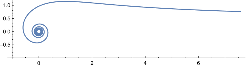
Figure 1. The algebraic spiral $\theta=\frac{3}{2}r^{-4/3}$ obtained by taking $c_{0}=1,\mu=3/4$.

We want to determine the relationship between $(\beta,\phi)$ and $(r,\theta)$, so that the new coordinates are adapted to our radially symmetric solutions. Since $\phi$ is constant along pseudo-streamlines, we can take

$$\phi=\theta-c_{0}\gamma^{-1}r^{-\frac{1}{\mu}},\qquad\beta=c_{0}\gamma^{-1}r^{-\frac{1}{\mu}}.$$

In this adapted coordinates, our radially symmetric solutions can be written as

$$\omega(\beta,\phi)=\gamma\beta,\qquad\psi(\beta,\phi)=c_{0}^{2\mu}\gamma^{-1-2\mu}\beta^{1-2\mu},\qquad\Omega(\phi)=c_{0}\mu^{\frac{1}{2\mu}}.$$

Since the value of $c_{0}$ does not affect the subsequent analysis, taking $c_{0}=\gamma\mu^{-\frac{1}{2\mu}}$ yields a special solution of the nonlinear equation (3.11):

(3.12) $$\psi_{0}=\frac{1}{2\mu-1}\beta^{1-2\mu},\qquad\Omega_{0}=\gamma.$$

4. Weighted functional spaces with $m$-fold symmetry

In this section, we introduce the functional framework for the implicit function theorem, which will be used to solve the nonlinear equation (3.11). In Subsection 4.1, we introduce some weighted Hölder type functional spaces for $\psi$ and $\Omega$. In Subsection 4.2, we introduce the functional spaces with $m$-fold symmetry and establish the Banach algebraic properties for these spaces.

4.1. Weighted Hölder type spaces

Given a continuous function $f=f(\beta,\phi):(0,+\infty)\times\mathbb{T}\to\mathbb{C}$ (we allow $f$ to be a single-variable function that depends only on the variable $\beta$) and $\alpha\in(0,1)$, we define the weighted Hölder norm of $f$ with respect to the variable $\beta$ by

$$\|f\|_{C_{\beta}^{\alpha}}: =\|\langle\beta\rangle^{\alpha}f\|_{L^{\infty}}+\sup_{\phi\in\mathbb{T}}\sup_{\begin{subarray}{c}0<\beta_{2}<\beta_{1}<2\beta_{2}\\ 0<|\beta_{1}-\beta_{2}|<1\end{subarray}}|\beta_{1}+\beta_{2}|^{\alpha}\frac{|f(\beta_{1},\phi)-f(\beta_{2},\phi)|}{|\beta_{1}-\beta_{2}|^{\alpha}}.$$

Here $\langle\beta\rangle=\sqrt{\beta^{2}+1}$.

In the sequel, we use the convention that if $\mathcal{X}$ and $\mathcal{Y}$ are Banach spaces embedded in the same linear Hausdorff space, then $\mathcal{X}+\mathcal{Y}$ is the Banach space with the induced norm

$$\|u\|_{\mathcal{X}+\mathcal{Y}}:=\inf\left\{\|x\|_{\mathcal{X}}+\|y\|_{\mathcal{Y}}:u=x+y,x\in\mathcal{X},y\in\mathcal{Y}\right\}.$$

Define $\mathcal{G}^{0}:=C_{\beta}^{\alpha}$ with the norm $\|f\|_{\mathcal{G}^{0}}:=\left\|f\right\|_{C_{\beta}^{\alpha}}$. We also define

$$\mathcal{G}^{-}:=\mathcal{G}^{0}\oplus\mathbb{C},\qquad\mathcal{G}:=\mathcal{G}^{0}\oplus C(\mathbb{T}).$$

Here we use $\oplus$ to denote the direct sums because $\mathcal{G}^{0}\cap\mathbb{C}=\mathcal{G}^{0}\cap C(\mathbb{T})=\{0\}$. Using the algebra properties of the space $C_{\beta}^{\alpha}$, Lemma 4.3 below, one can easily check that $\mathcal{G}$ is a unital Banach algebra and $\mathcal{G}^{0}$ is an ideal of $\mathcal{G}$, i.e., the embedding properties

(4.1) $$\mathcal{G}\cdot\mathcal{G}\hookrightarrow\mathcal{G},\qquad\mathcal{G}^{0}\cdot\mathcal{G}\hookrightarrow\mathcal{G}^{0}.$$

We introduce an auxiliary space $X_{0}$ defined by

$$X_{0}:=\left\{H=H(\beta,\phi):\ \beta^{2\mu}H_{\varphi},\beta^{2\mu-1}H_{\phi},\beta^{2\mu-1}H\in\mathcal{G}^{0}\right\}$$

with the norm

$$\|H\|_{X_{0}}:=\|\beta^{2\mu}H_{\varphi}\|_{\mathcal{G}^{0}}+\|\beta^{2\mu-1}H_{\phi}\|_{\mathcal{G}^{0}}+\|\beta^{2\mu-1}H\|_{\mathcal{G}^{0}};$$

and

$$X:=X_{0}\oplus\langle\beta^{1-2\mu}\rangle,$$

where $\langle\beta^{1-2\mu}\rangle$ is the one dimensional linear space generated by the function $\beta^{1-2\mu}$ with the standard norm.

Now we can define the functional space for $\psi$. Let

$$Y_{0}:=\left\{\psi=\psi(\beta,\phi):H=\psi+\frac{\beta}{2\mu}\psi_{\beta}\in X_{0},\beta^{2\mu-1}\psi\in C_{b}\right\}$$

with the norm

$$\|\psi\|_{Y_{0}}:=\left\|H\right\|_{X_{0}}+\|\beta^{2\mu-1}\psi\|_{L^{\infty}};$$

and we define

$$Y:=Y_{0}\oplus\langle\beta^{1-2\mu}\rangle.$$

Finally, the functional space for $\Omega$ is $\mathcal{W}:=L^{1}(\mathbb{T})$ and the target space is

(4.2) $$Z:=\Big{\{}G=G(\beta,\phi): \ G=\partial_{\varphi}F_{1}+\partial_{\phi}F_{2}\text{ weakly for some continuous functions}$$

$$\text{ $F_{1}$ and $F_{2}$ such that }\beta^{2\mu-1}F_{1}\in\mathcal{G}^{-},\beta^{2\mu}F_{2}\in\mathcal{G}^{0}\Big{\}}$$

with the norm

$$\|G\|_{Z}:=\inf\left(\|\beta^{2\mu-1}F_{1}\|_{\mathcal{G}^{-}}+\|\beta^{2\mu}F_{2}\|_{\mathcal{G}^{0}}\right),$$

where the infimum is taken over all decompositions of $G$ in (4.2). For further usage, we introduce an equivalent norm on $X_{0}$. Define the functional space

$$X_{0}^{\prime}:=\left\{H=H(\beta,\phi):\ \beta^{2\mu}H_{\varphi},\beta^{2\mu-1}H_{\phi}\in C_{\beta}^{\alpha},\langle\beta\rangle^{\alpha}\beta^{2\mu-1}H\in C_{b}\right\},$$

with the norm

$$\|H\|_{X_{0}^{\prime}}:=\|\beta^{2\mu}H_{\varphi}\|_{C_{\beta}^{\alpha}}+\|\beta^{2\mu-1}H_{\phi}\|_{C_{\beta}^{\alpha}}+\|\langle\beta\rangle^{\alpha}\beta^{2\mu-1}H\|_{L^{\infty}}.$$

Lemma 4.1.

The two functional spaces $X_{0}$ and $X_{0}^{\prime}$ are the same as sets, and their norms are equivalent:

$$\|H\|_{X_{0}}\sim\|H\|_{X_{0}^{\prime}},\qquad H\in X_{0}=X_{0}^{\prime}.$$

Proof.

Assume that $H\in X_{0}$, then by the definition of $C_{\beta}^{\alpha}$ norm,

$$\|\langle\beta\rangle^{\alpha}\beta^{2\mu-1}H\|_{L^{\infty}}\leq\|\beta^{2\mu-1}H\|_{C_{\beta}^{\alpha}}.$$

This proves $\|H\|_{X_{0}^{\prime}}\lesssim\|H\|_{X_{0}}$.

Assume that $H\in X_{0}^{\prime}$. Recall that $\partial_{\varphi}=\partial_{\phi}-\partial_{\beta}$, hence

$$\partial_{\beta}(\beta^{2\mu-1}H) =(2\mu-1)\beta^{-1}\beta^{2\mu-1}H+\beta^{2\mu-1}H_{\beta}$$

$$=(2\mu-1)\beta^{-1}\beta^{2\mu-1}H+\beta^{2\mu-1}H_{\phi}-\beta^{-1}\beta^{2\mu}H_{\varphi}.$$

By the definition of $C_{\beta}^{\alpha}$ norm, we have

$$\langle\beta\rangle^{\alpha}\left|\partial_{\beta}(\beta^{2\mu-1}H)\right| \leq\beta^{-1}\|\langle\beta\rangle^{\alpha}\beta^{2\mu-1}H\|_{L^{\infty}}+\|\langle\beta\rangle^{\alpha}\beta^{2\mu-1}H_{\phi}\|_{L^{\infty}}+\beta^{-1}\|\langle\beta\rangle^{\alpha}\beta^{2\mu}H_{\varphi}\|_{L^{\infty}}$$

$$\leq(1+\beta^{-1})\|H\|_{X_{0}^{\prime}}.$$

As a result, for $\beta_{1}>\beta_{2}>0$ with $\beta_{1}-\beta_{2}<1$, $\beta_{1}<2\beta_{2}$ and $\phi\in\mathbb{T}$, we have

$$\ \ \ \Big{|}\beta_{1}^{2\mu-1}H(\beta_{1},\phi)-\beta_{2}^{2\mu-1}H(\beta_{2},\phi)\Big{|}\leq\int_{\beta_{2}}^{\beta_{1}}\langle s\rangle^{-\alpha}\left(1+s^{-1}\right)\|H\|_{X_{0}^{\prime}}\,ds$$

$$\leq|\beta_{1}-\beta_{2}|\langle\beta_{2}\rangle^{-\alpha}\left(1+\beta_{2}^{-1}\right)\|H\|_{X_{0}^{\prime}}\leq\left(|\beta_{1}-\beta_{2}|/\beta_{2}+|\beta_{1}-\beta_{2}|/\beta_{2}^{\alpha}\right)\|H\|_{X_{0}^{\prime}}$$

$$\leq 2|\beta_{1}-\beta_{2}|^{\alpha}/\beta_{2}^{\alpha}\cdot\|H\|_{X_{0}^{\prime}}\lesssim|\beta_{1}-\beta_{2}|^{\alpha}/|\beta_{1}+\beta_{2}|^{\alpha}\cdot\|H\|_{X_{0}^{\prime}}.$$

Therefore, $\beta^{2\mu-1}H\in C_{\beta}^{\alpha}$ and $\|\beta^{2\mu-1}H\|_{C_{\beta}^{\alpha}}\lesssim\|H\|_{X_{0}^{\prime}}$. This proves $\|H\|_{X_{0}}\lesssim\|H\|_{X_{0}^{\prime}}$. ∎

As in the proof of $\beta^{2\mu-1}H\in C_{\beta}^{\alpha}$, we also have

(4.3) $$\|f\|_{C_{\beta}^{\alpha}}\lesssim\|\langle\beta\rangle^{\alpha}f\|_{L^{\infty}}+\|\langle\beta\rangle^{\alpha}(1+\beta^{-1})^{-1}\partial_{\beta}f\|_{L^{\infty}}\sim\|\langle\beta\rangle^{\alpha}f\|_{L^{\infty}}+\|\langle\beta\rangle^{\alpha-1}\beta\partial_{\beta}f\|_{L^{\infty}}.$$

To conclude this subsection, we prove some properties of the weighted Hölder space $C_{\beta}^{\alpha}$.

Lemma 4.2 (Equivalent norm on $C_{\beta}^{\alpha}$).

It holds that

(4.4) $$\|f\|_{C_{\beta}^{\alpha}}\sim\|\langle\beta\rangle^{\alpha}f\|_{L^{\infty}}+\sup_{\phi\in\mathbb{T}}\sup_{\begin{subarray}{c}\beta_{1}\neq\beta_{2}\\ \beta_{1},\beta_{2}>0\end{subarray}}|\beta_{1}+\beta_{2}|^{\alpha}\frac{|f(\beta_{1},\phi)-f(\beta_{2},\phi)|}{|\beta_{1}-\beta_{2}|^{\alpha}}.$$

Proof.

The “$\lesssim$” part is a direct consequence of the definition. We only need to prove the “$\gtrsim$” part. Let $\beta_{1},\beta_{2}>0$ be such that $\beta_{1}\neq\beta_{2}$. Without loss of generality, we assume that $0<\beta_{2}<\beta_{1}$. If $\beta_{1}<2\beta_{2}$ and $\beta_{1}-\beta_{2}<1$, then we get by the definition of the weighted Hölder norm that

$$|\beta_{1}+\beta_{2}|^{\alpha}\frac{|f(\beta_{1},\phi)-f(\beta_{2},\phi)|}{|\beta_{1}-\beta_{2}|^{\alpha}}\lesssim\|f\|_{C_{\beta}^{\alpha}}.$$

If $\beta_{1}<2\beta_{2}$ and $\beta_{1}-\beta_{2}\geq 1$, then

$$|\beta_{1}+\beta_{2}|^{\alpha}\frac{|f(\beta_{1},\phi)-f(\beta_{2},\phi)|}{|\beta_{1}-\beta_{2}|^{\alpha}}\leq(2\beta_{1})^{\alpha}|f(\beta_{1},\phi)|+(3\beta_{2})^{\alpha}|f(\beta_{2},\phi)|\lesssim\|\langle\beta\rangle^{\alpha}f\|_{L^{\infty}}\lesssim\|f\|_{C_{\beta}^{\alpha}}.$$

If $\beta_{1}\geq 2\beta_{2}$, then $\beta_{1}+\beta_{2}\leq 2\beta_{1}$ and $\beta_{1}-\beta_{2}\geq\frac{1}{2}\beta_{1}$, hence

$$|\beta_{1}+\beta_{2}|^{\alpha}\frac{|f(\beta_{1},\phi)-f(\beta_{2},\phi)|}{|\beta_{1}-\beta_{2}|^{\alpha}}\leq 4^{\alpha}\Big{(}\left|f(\beta_{1},\phi)\right|+\left|f(\beta_{2},\phi)\right|\Big{)}\lesssim\|f\|_{L^{\infty}}\lesssim\|\langle\beta\rangle^{\alpha}f\|_{L^{\infty}}\lesssim\|f\|_{C_{\beta}^{\alpha}}.$$

This completes the proof of the lemma. ∎

Lemma 4.3 (Algebra property).

Let $\alpha\in(0,1)$ and $f=f(\beta,\phi):(0,+\infty)\times\mathbb{T}\to\mathbb{R}$, $g=g(\beta,\phi):(0,+\infty)\times\mathbb{T}\to\mathbb{R}$.

1. If $\langle\beta\rangle^{-\alpha}f\in C_{\beta}^{\alpha}$ and $g\in C_{\beta}^{\alpha}$, then $fg\in C_{\beta}^{\alpha}$ and

   $$\|fg\|_{C_{\beta}^{\alpha}}\lesssim\|\langle\beta\rangle^{-\alpha}f\|_{C_{\beta}^{\alpha}}\|g\|_{C_{\beta}^{\alpha}}.$$

2. If $f\in C_{\beta}^{\alpha}$ and $g\in C_{\beta}^{\alpha}$, then $fg\in C_{\beta}^{\alpha}$ and

   $$\|fg\|_{C_{\beta}^{\alpha}}\lesssim\|f\|_{C_{\beta}^{\alpha}}\|g\|_{C_{\beta}^{\alpha}}.$$

Proof.

1. Firstly, we have

   $$\left\|\langle\beta\rangle^{\alpha}fg\right\|_{L^{\infty}}\leq\left\|f\right\|_{L^{\infty}}\left\|\langle\beta\rangle^{\alpha}g\right\|_{L^{\infty}}\leq\|\langle\beta\rangle^{-\alpha}f\|_{C_{\beta}^{\alpha}}\|g\|_{C_{\beta}^{\alpha}}.$$

   For simplicity, we denote $\tilde{f}=\langle\beta\rangle^{-\alpha}f$. For any $\beta_{1},\beta_{2}>0$ such that $0<\beta_{2}<\beta_{1}<2\beta_{2}$, $0<|\beta_{1}-\beta_{2}|<1$, we have

   $$\ \ \ \left|f(\beta_{1},\phi)g(\beta_{1},\phi)-f(\beta_{2},\phi)g(\beta_{2},\phi)\right|=\left|\langle\beta_{1}\rangle^{\alpha}\tilde{f}(\beta_{1},\phi)g(\beta_{1},\phi)-\langle\beta_{2}\rangle^{\alpha}\tilde{f}(\beta_{2},\phi)g(\beta_{2},\phi)\right|$$

   $$\qquad\leq\left|\tilde{f}(\beta_{1},\phi)-\tilde{f}(\beta_{2},\phi)\right|\langle\beta_{1}\rangle^{\alpha}|g(\beta_{1},\phi)|+\left|\langle\beta_{1}\rangle^{\alpha}-\langle\beta_{2}\rangle^{\alpha}\right|\left|\tilde{f}(\beta_{2},\phi)\right||g(\beta_{1},\phi)|$$

   $$\qquad\qquad\qquad\qquad+\langle\beta_{2}\rangle^{\alpha}\left|\tilde{f}(\beta_{2},\phi)\right|\left|g(\beta_{1},\phi)-g(\beta_{2},\phi)\right|$$

   $$\qquad\leq\frac{\left|\langle\beta_{1}\rangle^{\alpha}-\langle\beta_{2}\rangle^{\alpha}\right|}{\langle\beta_{1}\rangle^{\alpha}\langle\beta_{2}\rangle^{\alpha}}\left\|\tilde{f}\right\|_{C_{\beta}^{\alpha}}\|g\|_{C_{\beta}^{\alpha}}+2\frac{|\beta_{1}-\beta_{2}|^{\alpha}}{|\beta_{1}+\beta_{2}|^{\alpha}}\left\|\tilde{f}\right\|_{C_{\beta}^{\alpha}}\|g\|_{C_{\beta}^{\alpha}}\lesssim\frac{|\beta_{1}-\beta_{2}|^{\alpha}}{|\beta_{1}+\beta_{2}|^{\alpha}}\left\|\tilde{f}\right\|_{C_{\beta}^{\alpha}}\|g\|_{C_{\beta}^{\alpha}},$$

   where in the last inequality we used the fact

   $$\frac{\left|\langle\beta t\rangle^{\alpha}-\langle\beta\rangle^{\alpha}\right|}{\langle\beta t\rangle^{\alpha}\langle\beta\rangle^{\alpha}}\lesssim\frac{|t-1|^{\alpha}}{|t+1|^{\alpha}},\qquad\forall\ \beta>0,\forall\ t\in(1,2).$$

   Indeed, for all $\beta>0$ and $t\in(1,2)$, since $\left|\frac{d}{dt}\left(\langle\beta t\rangle^{\alpha}\right)\right|\leq\alpha\langle\beta t\rangle^{\alpha-1}\beta\leq\alpha\langle\beta\rangle^{\alpha-1}\beta$, we have

   $$\frac{\left|\langle\beta t\rangle^{\alpha}-\langle\beta\rangle^{\alpha}\right|}{\langle\beta t\rangle^{\alpha}\langle\beta\rangle^{\alpha}}\leq\frac{\alpha\langle\beta\rangle^{\alpha-1}\beta|t-1|}{\langle\beta\rangle^{\alpha}}\leq\alpha|t-1|\leq\alpha|t-1|^{\alpha}\leq\alpha 3^{\alpha}\frac{|t-1|^{\alpha}}{|t+1|^{\alpha}}.$$

2. It follows from (4.3) that

   $$\left\|\langle\beta\rangle^{-2\alpha}\right\|_{C_{\beta}^{\alpha}}\lesssim\left\|\langle\beta\rangle^{-\alpha}\right\|_{L^{\infty}}+\left\|\langle\beta\rangle^{\alpha-1}\beta\partial_{\beta}\left(\langle\beta\rangle^{-2\alpha}\right)\right\|_{L^{\infty}}\lesssim 1+\left\|\langle\beta\rangle^{\alpha-1}\beta^{2}\langle\beta\rangle^{-2\alpha-2}\right\|_{L^{\infty}}\lesssim 1.$$

   Hence, $\|\langle\beta\rangle^{-\alpha}f\|_{C_{\beta}^{\alpha}}\lesssim\left\|\langle\beta\rangle^{-2\alpha}\right\|_{C_{\beta}^{\alpha}}\left\|f\right\|_{C_{\beta}^{\alpha}}\lesssim\left\|f\right\|_{C_{\beta}^{\alpha}}$, and

   $$\|fg\|_{C_{\beta}^{\alpha}}\lesssim\|\langle\beta\rangle^{-\alpha}f\|_{C_{\beta}^{\alpha}}\|g\|_{C_{\beta}^{\alpha}}\lesssim\|f\|_{C_{\beta}^{\alpha}}\|g\|_{C_{\beta}^{\alpha}}.$$

This concludes the proof of the lemma. ∎

4.2. Functional spaces with $m$-fold symmetry

Given a positive integer $m$, we say a function $f=f(\beta,\phi):(0,+\infty)\times\mathbb{T}\to\mathbb{C}$ is $m$-fold symmetric if the following holds for all $(\beta,\phi)\in(0,+\infty)\times\mathbb{T}$:

$$f\left(\beta,\phi+\frac{2\pi}{m}\right)=f\left(\beta,\phi\right).$$

Note that if $f$ can be expressed in the form of Fourier series with respect to $\theta=\beta+\phi\in\mathbb{T}$:

$$f(\beta,\phi)=\sum_{n\in\mathbb{Z}}\hat{f}_{n}(\beta)e^{\mathrm{i}n(\beta+\phi)},\qquad\hat{f}_{n}(\beta):=\frac{1}{2\pi}\int_{\mathbb{T}}f(\beta,\phi)e^{-\mathrm{i}n(\beta+\phi)}\,d\phi,$$

then $f$ is $m$-fold symmetric if and only if $\hat{f}_{n}=0$ for all $n$ such that $m\nmid n$, that is to say,

$$f(\beta,\phi)=\sum_{n\in\mathbb{Z},m\mid n}\hat{f}_{n}(\beta)e^{\mathrm{i}n(\beta+\phi)}.$$

For notational convenience, we define the Fourier projections $P_{0}$ and $P_{\neq}$ by

$$(P_{0}f)(\beta):=\frac{1}{2\pi}\int_{\mathbb{T}}f(\beta,\phi)\,d\phi,\qquad(P_{\neq}f)(\beta,\phi):=f(\beta,\phi)-(P_{0}f)(\beta).$$

We start with the Banach algebras. Define

$$\mathcal{G}^{0}_{m}:=\left\{f=f(\beta,\phi)\in\mathcal{G}^{0}:f\text{ is $m$-fold symmetric}\right\}$$

with the norm

$$\|f\|_{\mathcal{G}_{m}^{0}}=\|P_{0}f\|_{\mathcal{G}^{0}}+m^{1/2}\|P_{\neq}f\|_{\mathcal{G}^{0}}.$$

Then $\|f\|_{C_{\beta}^{\alpha}}=\|f\|_{\mathcal{G}^{0}}\lesssim\|f\|_{\mathcal{G}_{m}^{0}}$.

Note that $P_{0},P_{\neq}$ are bounded linear operators on $\mathcal{G}^{0}$, since the Fourier projection is applied to the variable $\phi$. Also note that letting $m=1$ reproduces the space $\mathcal{G}^{0}$ defined in the previous subsection. We define

$$\mathcal{G}^{-}_{m}:=\mathcal{G}^{0}_{m}\oplus\mathbb{C},\qquad\mathcal{G}_{m}:=\mathcal{G}^{0}_{m}\oplus V_{m},$$

where $V_{m}=C_{m}(\mathbb{T}):=\{g=g(\phi)\in C(\mathbb{T}):g\text{ is $m$-fold symmetric}\}$ and

$$\|g\|_{V_{m}}:=|P_{0}g|+m^{1/2}\|P_{\neq}g\|_{L^{\infty}(\mathbb{T})}.$$

Note that if $g=g(\phi)\in C(\mathbb{T})$ then $P_{0}g$ is a complex number and $P_{\neq}g$ is a function in the variable $\phi$, with $\|g\|_{L^{\infty}(\mathbb{T})}\leq|P_{0}g|+\|P_{\neq}g\|_{L^{\infty}(\mathbb{T})}\lesssim\|g\|_{V_{m}}$.

Let’s show the Banach algebra properties of $\mathcal{G}_{m}^{0}$ and $\mathcal{G}_{m}$: $\mathcal{G}_{m}$ is a unital Banach algebra and $\mathcal{G}_{m}^{0}$ is an ideal of $\mathcal{G}_{m}$, i.e.,

$$\mathcal{G}_{m}\cdot\mathcal{G}_{m}\hookrightarrow\mathcal{G}_{m},\qquad\mathcal{G}_{m}^{0}\cdot\mathcal{G}_{m}\hookrightarrow\mathcal{G}_{m}^{0},$$

where the embeddings are uniform in $m\in\mathbb{N}_{+}$. In this paper, all embeddings of spaces varying with $m\in\mathbb{N}_{+}$ are uniform in $m\in\mathbb{N}_{+}$.

Lemma 4.4.

We have the following embeddings which are uniform in $m\in\mathbb{N}_{+}$:

(4.5) $$\mathcal{G}_{m}^{0}\cdot\mathcal{G}_{m}^{0} \hookrightarrow\mathcal{G}_{m}^{0},$$

(4.6) $$\mathcal{G}_{m}^{0}\cdot V_{m} \hookrightarrow\mathcal{G}_{m}^{0},$$

(4.7) $$V_{m}\cdot V_{m} \hookrightarrow V_{m},$$

(4.8) $$\mathcal{G}_{m}^{0}\cdot\mathcal{G}_{m} \hookrightarrow\mathcal{G}_{m}^{0},$$

(4.9) $$\mathcal{G}_{m}\cdot\mathcal{G}_{m} \hookrightarrow\mathcal{G}_{m}.$$

Proof.

Let $f_{1}=f_{1}(\beta,\phi)\in\mathcal{G}_{m}^{0}$ and $f_{2}=f_{2}(\beta,\phi)\in\mathcal{G}_{m}^{0}$. Recall that $P_{0}$ is the Fourier projection applied to the variable $\phi$. By Lemma 4.3, we obtain

$$\|P_{0}(f_{1}f_{2})\|_{C_{\beta}^{\alpha}}\lesssim\|f_{1}f_{2}\|_{C_{\beta}^{\alpha}}\lesssim\|f_{1}\|_{C_{\beta}^{\alpha}}\|f_{2}\|_{C_{\beta}^{\alpha}}\lesssim\|f_{1}\|_{\mathcal{G}_{m}^{0}}\|f_{2}\|_{\mathcal{G}_{m}^{0}}.$$

As for $P_{\neq}(f_{1}f_{2})$, noting that

$$P_{\neq}(f_{1}f_{2})=P_{0}f_{1}\cdot P_{\neq}f_{2}+P_{0}f_{2}\cdot P_{\neq}f_{1}+P_{\neq}\left(P_{\neq}f_{1}\cdot P_{\neq}f_{2}\right),$$

we get by Lemma 4.3 that

$$\|P_{\neq}(f_{1}f_{2})\|_{C_{\beta}^{\alpha}} \lesssim\|P_{0}f_{1}\|_{C_{\beta}^{\alpha}}\|P_{\neq}f_{2}\|_{C_{\beta}^{\alpha}}+\|P_{0}f_{2}\|_{C_{\beta}^{\alpha}}\|P_{\neq}f_{1}\|_{C_{\beta}^{\alpha}}+\|P_{\neq}f_{1}\|_{C_{\beta}^{\alpha}}\|P_{\neq}f_{2}\|_{C_{\beta}^{\alpha}}$$

$$\lesssim m^{-1/2}\|f_{1}\|_{\mathcal{G}_{m}^{0}}\|f_{2}\|_{\mathcal{G}_{m}^{0}}.$$

Therefore, we have $\|f_{1}f_{2}\|_{\mathcal{G}_{m}^{0}}\lesssim\|f_{1}\|_{\mathcal{G}_{m}^{0}}\|f_{2}\|_{\mathcal{G}_{m}^{0}}$. This shows (4.5).

The proof of (4.6) is very similar to (4.5),with the algebraic properties of $C_{\beta}^{\alpha}$ replaced by the trivial embedding $C_{\beta}^{\alpha}\cdot C(\mathbb{T})\hookrightarrow C_{\beta}^{\alpha}$. The proof of (4.7) is very similar to (4.5) and we only need to replace the algebraic properties of $C_{\beta}^{\alpha}$ by the trivial embedding $C(\mathbb{T})\cdot C(\mathbb{T})\hookrightarrow C(\mathbb{T})$. (4.8) follows directly from the definition $\mathcal{G}_{m}=\mathcal{G}^{0}_{m}\oplus V_{m}$ and (4.5), (4.6).

Now we prove (4.9). By (4.8), we have $\mathcal{G}_{m}^{0}\cdot\mathcal{G}_{m}\hookrightarrow\mathcal{G}_{m}^{0}\hookrightarrow\mathcal{G}_{m}$. It remains to show that $V_{m}\cdot\mathcal{G}_{m}\hookrightarrow\mathcal{G}_{m}$, which follows directly from the definition $\mathcal{G}_{m}=\mathcal{G}^{0}_{m}\oplus V_{m}$ and (4.6), (4.7). ∎

Now we define the $m$-fold version of the spaces $X$ and $Y$. Let

$$X_{0,m}:=\left\{H=H(\beta,\phi)\in X_{0}:H\text{ is $m$-fold symmetric}\right\}$$

with the norm

$$\|H\|_{X_{0,m}}:=\|P_{0}H\|_{X_{0}}+m^{1/2}\|P_{\neq}H\|_{X_{0}},$$

and we define $X_{m}:=X_{0,m}\oplus\langle\beta^{1-2\mu}\rangle$. Note that letting $m=1$ we recover the spaces $X_{0}$ and $X$ defined previously. Let

$$Y_{0,m}:=\left\{\psi=\psi(\beta,\phi)\in Y_{0}:\psi\text{ is $m$-fold symmetric}\right\}$$

with the norm

$$\|\psi\|_{Y_{0,m}}:=\|P_{0}\psi\|_{Y_{0}}+m^{1/2}\|P_{\neq}\psi\|_{Y_{0}},$$

and we define $Y_{m}:=Y_{0,m}\oplus\langle\beta^{1-2\mu}\rangle$. Note that letting $m=1$ we recover the spaces $Y_{0}$ and $Y$ defined previously.

Finally, the functional space for $m$-fold $\Omega$ is

$$\mathcal{W}_{m}:=L^{1}_{m}(\mathbb{T}):=\left\{\Omega=\Omega(\phi)\in L^{1}(\mathbb{T}):\Omega\text{ is $m$-fold symmetric}\right\},$$

with the norm

$$\|\Omega\|_{\mathcal{W}_{m}}:=|P_{0}\Omega|+m^{-1/2}\|P_{\neq}\Omega\|_{L^{1}(\mathbb{T})}.$$

Then $\|\Omega\|_{L^{1}(\mathbb{T})}\lesssim m^{1/2}\|\Omega\|_{\mathcal{W}_{m}}$. And the target space is

(4.10) $$Z_{m}: =\Big{\{}G=G(\beta,\phi):G=\partial_{\varphi}F_{1}+\partial_{\phi}F_{2}\text{ weakly for some continuous $m$-fold}$$

$$\qquad\ \ \text{functions $F_{1}$ and $F_{2}$ such that }\beta^{2\mu-1}F_{1}\in\mathcal{G}_{m}^{-},\beta^{2\mu}F_{2}\in\mathcal{G}_{m}^{0}\Big{\}}$$

with the norm

$$\|G\|_{Z_{m}}:=\inf\left(\|\beta^{2\mu-1}F_{1}\|_{\mathcal{G}_{m}^{-}}+\|\beta^{2\mu}F_{2}\|_{\mathcal{G}_{m}^{0}}\right),$$

where the infimum is taken over all decompositions of $G$ in (4.10).

A remarkable property of these functional spaces is the following proposition.

Proposition 4.5.

For $\alpha\in(0,1)$ and $\mu>\frac{1}{2}$, the following embeddings are uniform in $m\in\mathbb{N}_{+}$:

(4.11) $$V_{m}\cdot\mathcal{W}_{m} \hookrightarrow\mathcal{W}_{m},$$

(4.12) $$\beta^{-2\mu}\mathcal{G}_{m}^{0}\cdot\mathcal{W}_{m} \hookrightarrow Z_{m},$$

(4.13) $$\beta^{-2\mu}\mathcal{W}_{m} \hookrightarrow Z_{m},$$

(4.14) $$\beta^{-2\mu}\mathcal{G}_{m}\cdot\mathcal{W}_{m} \hookrightarrow Z_{m}.$$

To prove Proposition 4.5, the following Lemma is useful.

Lemma 4.6.

Let $f=f(\phi)\in L^{1}(\mathbb{T})$ be an $m$-fold symmetric integrable function defined on $\mathbb{T}=\mathbb{R}/2\pi\mathbb{Z}$, where $m\geq 1$ is a positive integer, such that $\int_{\mathbb{T}}f(\phi)\,d\phi=0$. Then there exists $g\in C_{m}(\mathbb{T})$ such that $f=g^{\prime}$ almost everywhere, $\int_{\mathbb{T}}g(\phi)\,d\phi=0$ and

$$\|g\|_{L^{\infty}(\mathbb{T})}\leq\frac{C}{m}\|f\|_{L^{1}(\mathbb{T})},$$

where $C>0$ is an absolute constant independent of $m$ and $f$.

Proof.

Define

$$g_{0}(\phi)=\int_{0}^{\phi}f(\Phi)\,d\Phi,\qquad\phi\in\mathbb{T}.$$

Since $f\in L^{1}(\mathbb{T})$ and $\int_{\mathbb{T}}f(\phi)\,d\phi=0$, it is easy to check that $g_{0}$ is $2\pi$-periodic, hence $g_{0}$ is a well-defined continuous function on $\mathbb{T}$, and moreover, we have $\|g_{0}\|_{L^{\infty}(\mathbb{T})}\leq\|f\|_{L^{1}(\mathbb{T})}$ and $g^{\prime}=f$ a.e.. It follows from the $\frac{2\pi}{m}$-periodic property of $f$ and $\int_{\mathbb{T}}f(\phi)\,d\phi=0$ that

$$\int_{\phi}^{\phi+\frac{2\pi}{m}}f(\Phi)\,d\Phi=0,\qquad\phi\in\mathbb{T}.$$

As a result, by the definition of $g$, we have

$$g_{0}\left(\phi+\frac{2\pi}{m}\right)=g_{0}(\phi)+\int_{\phi}^{\phi+\frac{2\pi}{m}}f(\Phi)\,d\Phi=g_{0}(\phi),\qquad\phi\in\mathbb{T},$$

which implies that $g_{0}$ is $m$-fold symmetric, hence $g_{0}\in C_{m}(\mathbb{T})$. Now we show that $|g_{0}(\phi)|\leq\frac{1}{m}\|f\|_{L^{1}(\mathbb{T})}$ for $\phi\in\mathbb{T}$. Due to the $m$-fold symmetry of $g_{0}$, we can assume without loss of generality that $\phi\in\left[0,\frac{2\pi}{m}\right)$. By the periodicity of $f$, we have

$$g_{0}(\phi)=\frac{1}{m}\int_{0}^{\phi}\sum_{k=0}^{m-1}f\left(\Phi+\frac{2\pi}{m}\right)\,d\Phi=\frac{1}{m}\int_{\bigcup_{k=0}^{m-1}\left[k\frac{2\pi}{m},\phi+k\frac{2\pi}{m}\right]}f(\Phi)\,d\Phi,$$

therefore,

$$\left|g_{0}(\phi)\right|\leq\frac{1}{m}\|f\|_{L^{1}(\mathbb{T})},\qquad\forall\ \phi\in\mathbb{T}.$$

Finally, let $g=P_{\neq}g_{0}$, then $g$ and $g_{0}$ differ by only a constant, hence $g\in C_{m}(\mathbb{T})$, $f=g^{\prime}$ almost everywhere and

$$\|g\|_{L^{\infty}(\mathbb{T})}\leq|P_{0}g_{0}|+\|g_{0}\|_{L^{\infty}(\mathbb{T})}\leq C\|g_{0}\|_{L^{\infty}(\mathbb{T})}\leq\frac{C}{m}\|f\|_{L^{1}(\mathbb{T})}.$$

The proof of the lemma is complete. ∎

In fact, $g$ is unique and $f\mapsto g$ is a linear operator. Now we are ready to prove Proposition 4.5.

Proof of Proposition 4.5.

Step 1. Proof of (4.11). Let $g=g(\phi)\in V_{m}$ and $\Omega=\Omega(\phi)\in\mathcal{W}_{m}$. Since

$$P_{0}(g\Omega)=P_{0}g\cdot P_{0}\Omega+P_{0}(P_{\neq}g\cdot P_{\neq}\Omega),$$

and $P_{0}$ is a bounded linear functional on $L^{1}(\mathbb{T})$, we have

$$|P_{0}(g\Omega)| \lesssim|P_{0}g||P_{0}\Omega|+\left\|P_{\neq}g\cdot P_{\neq}\Omega\right\|_{L^{1}(\mathbb{T})}\lesssim|P_{0}g||P_{0}\Omega|+\|P_{\neq}g\|_{L^{\infty}(\mathbb{T})}\|P_{\neq}\Omega\|_{L^{1}(\mathbb{T})}$$

$$\lesssim\|g\|_{V_{m}}\|\Omega\|_{\mathcal{W}_{m}}+m^{-1/2}\|g\|_{V_{m}}\cdot m^{1/2}\|\Omega\|_{\mathcal{W}_{m}}\lesssim\|g\|_{V_{m}}\|\Omega\|_{\mathcal{W}_{m}}.$$

For $P_{\neq}(g\Omega)$, we have

$$\|P_{\neq}(g\Omega)\|_{L^{1}(\mathbb{T})} \lesssim\|g\Omega\|_{L^{1}(\mathbb{T})}+|P_{0}(g\Omega)|\lesssim\|g\|_{L^{\infty}(\mathbb{T})}\|\Omega\|_{L^{1}(\mathbb{T})}+\|g\|_{V_{m}}\|\Omega\|_{\mathcal{W}_{m}}$$

$$\lesssim m^{1/2}\|g\|_{V_{m}}\|\Omega\|_{\mathcal{W}_{m}}.$$

Hence, $g\Omega\in\mathcal{W}_{m}$ and $\|g\Omega\|_{\mathcal{W}_{m}}\lesssim\|g\|_{V_{m}}\|\Omega\|_{\mathcal{W}_{m}}.$

Step 2. Proof of (4.12). Let $f=f(\beta,\phi)\in\mathcal{G}_{m}^{0}$ and $\Omega=\Omega(\phi)\in\mathcal{W}_{m}$. Denote

$$f_{0}(\beta):=P_{0}(f\Omega)(\beta)=P_{0}f(\beta)\cdot P_{0}\Omega+P_{0}(P_{\neq}f\cdot P_{\neq}\Omega)(\beta).$$

Then we have $f_{0}\in C_{\beta}^{\alpha}$ and

$$\|f_{0}\|_{C_{\beta}^{\alpha}}\lesssim\|P_{0}f\|_{C_{\beta}^{\alpha}}|P_{0}\Omega|+\|P_{\neq}f\|_{C_{\beta}^{\alpha}}\|P_{\neq}\Omega\|_{L^{1}(\mathbb{T})}\lesssim\|f\|_{\mathcal{G}_{m}^{0}}\|\Omega\|_{\mathcal{W}_{m}}.$$

By Lemma 4.6, there exists an $m$-fold function $f_{1}=f_{1}(\beta,\phi)$ such that ${{P_{0}f_{1}=0}}$, $P_{\neq}(f\Omega)=\partial_{\phi}f_{1}$ and

$$|f_{1}(\beta,\phi)|\lesssim\frac{1}{m}\int_{\mathbb{T}}|P_{\neq}(f\Omega)|(\beta,\Phi)d\Phi\lesssim\frac{1}{m}\int_{\mathbb{T}}|f\Omega|(\beta,\Phi)d\Phi\leq\frac{1}{m}\sup_{\Phi\in\mathbb{T}}|f(\beta,\Phi)|\|\Omega\|_{L^{1}(\mathbb{T})},$$

$$|f_{1}(\beta_{1},\phi)-f_{1}(\beta_{2},\phi)|\lesssim\frac{1}{m}\int_{\mathbb{T}}|P_{\neq}(f\Omega)(\beta_{1},\Phi)-P_{\neq}(f\Omega)(\beta_{2},\Phi)|d\Phi$$

$$\lesssim\frac{1}{m}\int_{\mathbb{T}}|(f\Omega)(\beta_{1},\Phi)-(f\Omega)(\beta_{2},\Phi)|d\Phi\leq\frac{1}{m}\sup_{\Phi\in\mathbb{T}}|f(\beta_{1},\Phi)-f(\beta_{2},\Phi)|\|\Omega\|_{L^{1}(\mathbb{T})}.$$

Then by the definition of the $C_{\beta}^{\alpha}$ norm, we have $f_{1}\in C_{\beta}^{\alpha}$ with

$$\|f_{1}\|_{C_{\beta}^{\alpha}}\lesssim\frac{1}{m}\|f\|_{C_{\beta}^{\alpha}}\|\Omega\|_{L^{1}(\mathbb{T})}\lesssim m^{-1/2}\|f\|_{\mathcal{G}_{m}^{0}}\|\Omega\|_{\mathcal{W}_{m}}.$$

Hence, we have

$$\beta^{-2\mu}f(\beta,\phi)\Omega(\phi) =\beta^{-2\mu}f_{0}(\beta)+\partial_{\phi}(\beta^{-2\mu}f_{1}(\beta,\phi))$$

$$=\partial_{\varphi}\left(\int_{\beta}^{\infty}s^{-2\mu}f_{0}(s)\,ds\right)+\partial_{\phi}(\beta^{-2\mu}f_{1}(\beta,\phi))$$

$$=:\partial_{\varphi}F_{1}+\partial_{\phi}F_{2},$$

where $F_{1}=P_{0}F_{1}$ and $F_{2}=P_{\neq}F_{2}$. For $F_{2}$, there holds

$$\|\beta^{2\mu}F_{2}\|_{\mathcal{G}_{m}^{0}}=m^{1/2}\|\beta^{2\mu}F_{2}\|_{C_{\beta}^{\alpha}}=m^{1/2}\|f_{1}\|_{C_{\beta}^{\alpha}}\lesssim\|f\|_{\mathcal{G}_{m}^{0}}\|\Omega\|_{\mathcal{W}_{m}}.$$

For $F_{1}=F_{1}(\beta)=\int_{\beta}^{\infty}s^{-2\mu}f_{0}(s)\,ds$, we have

$$\left|\langle\beta\rangle^{\alpha}\beta^{2\mu-1}F_{1}(\beta)\right|\lesssim\langle\beta\rangle^{\alpha}\beta^{2\mu-1}\left(\int_{\beta}^{\infty}\langle s\rangle^{-\alpha}s^{-2\mu}\,ds\right)\|\langle\beta\rangle^{\alpha}f_{0}\|_{L^{\infty}}\lesssim\|\langle\beta\rangle^{\alpha}f_{0}\|_{L^{\infty}};$$

and

$$\left|\partial_{\beta}\left(\beta^{2\mu-1}F_{1}\right)\right| \lesssim\beta^{2\mu-2}\left(\int_{\beta}^{\infty}s^{-2\mu}\,ds\right)\|f_{0}\|_{L^{\infty}}+\beta^{-1}\|f_{0}\|_{L^{\infty}}\lesssim\beta^{-1}\|f_{0}\|_{L^{\infty}}$$

Then by (4.3) and $\langle\beta\rangle^{\alpha}\geq 1\geq\langle\beta\rangle^{\alpha-1}$, we have $\beta^{2\mu-1}F_{1}\in C_{\beta}^{\alpha}$ and

$$\|\beta^{2\mu-1}F_{1}\|_{\mathcal{G}_{m}^{-}}=\|\beta^{2\mu-1}F_{1}\|_{C_{\beta}^{\alpha}}\lesssim\|\langle\beta\rangle^{\alpha}f_{0}\|_{L^{\infty}}\leq\|f_{0}\|_{C_{\beta}^{\alpha}}\lesssim\|f\|_{\mathcal{G}_{m}^{0}}\|\Omega\|_{\mathcal{W}_{m}}.$$

Therefore, $\beta^{-2\mu}f\Omega\in Z_{m}$ and

$$\|\beta^{-2\mu}f\Omega\|_{Z_{m}}\lesssim\|\beta^{2\mu-1}F_{1}\|_{\mathcal{G}_{m}^{-}}+\|\beta^{2\mu}F_{2}\|_{\mathcal{G}_{m}^{0}}\lesssim\|f\|_{\mathcal{G}_{m}^{0}}\|\Omega\|_{\mathcal{W}_{m}}.$$

Step 3. Proof of (4.13). Let $\Omega=\Omega(\phi)\in\mathcal{W}_{m}$. By Lemma 4.6, we can find $g,h\in C_{m}(\mathbb{T})$ such that $P_{0}g=P_{0}h=0$, $P_{\neq}\Omega=\partial_{\phi}g=\partial_{\phi}^{2}h$ and

$$\|g\|_{L^{\infty}(\mathbb{T})}\lesssim\frac{1}{m}\|P_{\neq}\Omega\|_{L^{1}(\mathbb{T})},\qquad\|h\|_{L^{\infty}(\mathbb{T})}\lesssim\frac{1}{m^{2}}\|P_{\neq}\Omega\|_{L^{1}(\mathbb{T})}.$$

We introduce a smooth bump function

(4.15) $$\rho\in C^{\infty}([0,\infty);[0,1])\qquad\text{ such that }\qquad\rho(\beta)=\begin{cases}0&\beta\in[0,1],\\ 1&\beta\geq 2.\end{cases}$$

Due to $\partial_{\varphi}=\partial_{\phi}-\partial_{\beta}$, we obtain

$$\beta^{-2\mu}\Omega(\phi) =\beta^{-2\mu}P_{0}\Omega+\beta^{-2\mu}\partial_{\phi}g=P_{0}\Omega\partial_{\varphi}\left(\frac{1}{2\mu-1}\beta^{1-2\mu}\right)+\partial_{\phi}\left(\beta^{-2\mu}g(\phi)\right)$$

$$=\partial_{\varphi}\left(\frac{P_{0}\Omega}{2\mu-1}\beta^{1-2\mu}\right)+\partial_{\phi}\Big{(}(1-\rho(\beta))\beta^{-2\mu}g(\phi)\Big{)}+\left(\partial_{\varphi}+\partial_{\beta}\right)\Big{(}\rho(\beta)\beta^{-2\mu}g(\phi)\Big{)}$$

$$=\partial_{\varphi}\left(\frac{P_{0}\Omega}{2\mu-1}\beta^{1-2\mu}+\rho(\beta)\beta^{-2\mu}g(\phi)\right)$$

$$\qquad\qquad+\partial_{\phi}\Big{(}(1-\rho(\beta))\beta^{-2\mu}g(\phi)+\partial_{\beta}(\rho(\beta)\beta^{-2\mu})h(\phi)\Big{)}$$

$$=:\partial_{\varphi}G_{1}+\partial_{\phi}G_{2}.$$

We also have the following estimates: for $G_{1}$

$$\|\beta^{2\mu-1}G_{1}\|_{\mathcal{G}_{m}^{-}} =\|\beta^{2\mu-1}P_{0}G_{1}\|_{\mathcal{G}^{-}}+m^{1/2}\|\beta^{2\mu-1}P_{\neq}{G_{1}}\|_{\mathcal{G}^{-}}$$

$$=\left|\frac{P_{0}\Omega}{2\mu-1}\right|+m^{1/2}\left\|\frac{\rho(\beta)}{\beta}g\right\|_{\mathcal{G}^{0}}\lesssim|P_{0}\Omega|+m^{1/2}\|g\|_{L^{\infty}(\mathbb{T})}$$

$$\lesssim|P_{0}\Omega|+m^{-1/2}\|P_{\neq}\Omega\|_{L^{1}(\mathbb{T})}\lesssim\|\Omega\|_{\mathcal{W}_{m}},$$

and for ${G_{2}}$, noting that $P_{0}{G_{2}}=0$

$$\|\beta^{2\mu}{G_{2}}\|_{\mathcal{G}_{m}^{0}} =m^{1/2}\|\beta^{2\mu}{G_{2}}\|_{\mathcal{G}^{0}}\lesssim m^{1/2}\left(\|g\|_{L^{\infty}(\mathbb{T})}+\|h\|_{L^{\infty}(\mathbb{T})}\right)$$

$$\lesssim m^{-1/2}\|P_{\neq}\Omega\|_{L^{1}(\mathbb{T})}\lesssim\|\Omega\|_{\mathcal{W}_{m}}.$$

Therefore, $\beta^{-2\mu}\Omega\in Z_{m}$ and $\|\beta^{-2\mu}\Omega\|_{Z_{m}}\lesssim\|\Omega\|_{\mathcal{W}_{m}}.$

Finally, (4.14) follows directly from the definition $\mathcal{G}_{m}=\mathcal{G}_{m}^{0}\oplus V_{m}$ and (4.11)$\sim$(4.13). ∎

5. Nonlinear problem in the adapted coordinates

Let $m\geq 1$ be a positive integer. Given $\psi\in Y_{m}$ and $\Omega\in\mathcal{W}_{m}$, recall the nonlinear map

(5.1) $$\mathcal{F}(\psi,\Omega)=\partial_{\varphi}\mathcal{N}_{1}(\psi)+\partial_{\phi}\mathcal{N}_{2}(\psi)+\mathcal{N}_{3}(\psi)\Omega,$$

where

$$\mathcal{N}_{1}(\psi)=\frac{2\psi_{\beta}\psi_{\varphi}}{\psi_{\beta\varphi}}-\frac{\psi_{\beta\phi}}{\psi_{\beta\varphi}}\mathcal{N}_{2}(\psi),\ \ \mathcal{N}_{2}(\psi)=\frac{\psi_{\beta\varphi}\psi_{\phi}-\psi_{\beta\phi}\psi_{\varphi}}{2\psi_{\beta}},\ \ \mathcal{N}_{3}(\psi)=\frac{\psi_{\beta\varphi}\psi_{\varphi}^{-\frac{1}{2\mu}}}{2\mu}.$$

By (3.12) we have $\mathcal{F}(\psi_{0},\Omega_{0})=0$. Recall that we are going to solve the equation $\mathcal{F}(\psi,\Omega)=0$ to get the solution $\psi=\psi(\Omega)$ for $\Omega$ near $\Omega_{0}=\gamma$.

As we mentioned before, a natural idea is to use the implicit function theorem (see Theorem 1.2.1 in [7] for example). For a Banach space $\mathcal{X}$, $x_{0}\in\mathcal{X}$ and a positive number $\delta>0$, we denote by $B_{\delta}^{(\mathcal{X})}(x_{0})$ the ball in $\mathcal{X}$ of radius $\delta$ around $x_{0}$. Given $\mu>\frac{1}{2}$, we define

(5.2) $$\alpha_{\mu}:=\sqrt{4\mu^{2}-2\mu+1}-(2\mu-1)\in\left(\frac{1}{2},1\right).$$

The main result of this section is stated as follows.

Theorem 5.1.

Assume that $m\geq 2$, $\mu>\frac{1}{2}$ and $\alpha\in\left(0,\alpha_{\mu}\right)$, where $\alpha_{\mu}$ is given by (5.2). There exist $\varepsilon_{\psi},\varepsilon_{\Omega}>0$ independent of $m\geq 2$ and a unique $C^{2}$ map $\Xi:B_{\varepsilon_{\Omega}}^{(\mathcal{W}_{m})}(\Omega_{0})\to B_{\varepsilon_{\psi}}^{(Y_{m})}(\psi_{0})$ such that

$$\mathcal{F}(\psi,\Omega)=0,(\psi,\Omega)\in B_{\varepsilon_{\psi}}^{(Y_{m})}(\psi_{0})\times B_{\varepsilon_{\Omega}}^{(\mathcal{W}_{m})}(\Omega_{0})\ \ \Longleftrightarrow\ \ \ \psi=\Xi(\Omega).$$

Moreover, $\Xi(\Omega)$ is real-valued if $\Omega$ is real-valued.

Remark 5.2.

In fact, we can show that $\mathcal{F}$ is $C^{\infty}$, therefore $\Xi:B_{\varepsilon_{\Omega}}^{(\mathcal{W}_{m})}(\Omega_{0})\to B_{\varepsilon_{\psi}}^{(Y_{m})}(\psi_{0})$ is also $C^{\infty}$.

5.1. $C^{2}$ regularity of nonlinear map

Proposition 5.3.

Assume that $\alpha\in(0,1)$, $m\in\mathbb{N}_{+}$ and $\mu>\frac{1}{2}$. There exists $\delta>0$, which is a small constant independent of $m\in\mathbb{N}_{+}$, such that

$$\mathcal{F}\in C^{2}\Big{(}B_{\delta}^{(Y_{m})}(\psi_{0})\times\mathcal{W}_{m};Z_{m}\Big{)},$$

and the $C^{2}$ norm of $\mathcal{F}$ is independent of $m\in\mathbb{N}_{+}$.

Throughout this subsection, we assume that $\alpha\in(0,1)$, $m\in\mathbb{N}_{+}$ and $\mu>\frac{1}{2}$.

Lemma 5.4.

Let $H\in X_{0}$ and

(5.3) $$F(\beta,\phi)=2\mu\beta^{-2\mu}\int_{0}^{\beta}s^{2\mu-1}H(s,\phi)\,ds,\qquad(\beta,\phi)\in(0,+\infty)\times\mathbb{T}.$$

Then $F$ is the unique function in $Y_{0}$ such that $H=F+\frac{\beta}{2\mu}F_{\beta}$ and

$$\ \|F\|_{Y_{0}}+\|\beta^{2\mu}F_{\beta\phi}\|_{C_{\beta}^{\alpha}}+\|\beta^{2\mu}F_{\beta}\|_{C_{\beta}^{\alpha}}+\|\beta^{2\mu-1}F_{\phi}\|_{C_{\beta}^{\alpha}}+\|\beta^{2\mu-1}F\|_{C_{\beta}^{\alpha}}\lesssim\|H\|_{X_{0}}.$$

For further usage, we denote by $T_{0}$ the map from $H$ to $F$, then $T_{0}:X_{0}\to Y_{0}$ is a bounded linear operator.

Proof.

Clearly, $F$ is well-defined, i.e., the integral in (5.3) is absolutely convergent. Direct computation gives the identity $H=F+\frac{\beta}{2\mu}F_{\beta}$ and the uniqueness is also trivial. For simplicity, we omit the variable $\phi$ here in this proof.

1. $\|F\|_{Y_{0}}+\|\beta^{2\mu-1}F\|_{C_{\beta}^{\alpha}}\lesssim\|H\|_{X_{0}}$. For any $\beta>0$, we have

   $$|\langle\beta\rangle^{\alpha}\beta^{2\mu-1}F(\beta)|\lesssim\langle\beta\rangle^{\alpha}\beta^{-1}\left(\int_{0}^{\beta}\langle s\rangle^{-\alpha}\,ds\right)\|\langle\beta\rangle^{\alpha}\beta^{2\mu-1}H\|_{L^{\infty}}\lesssim\|\langle\beta\rangle^{\alpha}\beta^{2\mu-1}H\|_{L^{\infty}},$$

   and

   $$\left|\partial_{\beta}\left(\beta^{2\mu-1}F\right)(\beta)\right| \lesssim\beta^{-2}\int_{0}^{\beta}s^{2\mu-1}|H(s)|\,ds+\beta^{-1}|\beta^{2\mu-1}H(\beta)|$$

   $$\lesssim\beta^{-1}\|\beta^{2\mu-1}H\|_{L^{\infty}}\lesssim\beta^{-1}\|\langle\beta\rangle^{\alpha}\beta^{2\mu-1}H\|_{L^{\infty}}.$$

   Therefore, by (4.3), we have $\beta^{2\mu-1}F\in C_{\beta}^{\alpha}$ and

   $$\|\beta^{2\mu-1}F\|_{C_{\beta}^{\alpha}}\lesssim\|\langle\beta\rangle^{\alpha}\beta^{2\mu-1}H\|_{L^{\infty}}\lesssim\|\beta^{2\mu-1}H\|_{C_{\beta}^{\alpha}}\lesssim\|H\|_{X_{0}}.$$

   We also have

   $$\|F\|_{Y_{0}}=\|H\|_{X_{0}}+\|\beta^{2\mu-1}F\|_{L^{\infty}}\lesssim\|H\|_{X_{0}}+\|\beta^{2\mu-1}F\|_{C_{\beta}^{\alpha}}\lesssim\|H\|_{X_{0}}.$$

2. $\|\beta^{2\mu-1}F_{\phi}\|_{C_{\beta}^{\alpha}}\lesssim\|H\|_{X_{0}}$. The same argument as in $(1)$ gives that $\beta^{2\mu-1}F_{\phi}\in C_{\beta}^{\alpha}$ and $\|\beta^{2\mu-1}F_{\phi}\|_{C_{\beta}^{\alpha}}\lesssim\|\beta^{2\mu-1}H_{\phi}\|_{C_{\beta}^{\alpha}}\lesssim\|H\|_{X_{0}}$ (as $F=T_{0}H\Rightarrow F_{\phi}=T_{0}H_{\phi}$).

3. $\|\beta^{2\mu}F_{\beta}\|_{C_{\beta}^{\alpha}}\lesssim\|H\|_{X_{0}}$. The identity $H=F+\frac{\beta}{2\mu}F_{\beta}$ implies $F_{\beta}=2\mu\beta^{-1}H-2\mu\beta^{-1}F$, hence $\beta^{2\mu}F_{\beta}=2\mu\beta^{2\mu-1}H-2\mu\beta^{2\mu-1}F\in C_{\beta}^{\alpha}$ and

   $$\|\beta^{2\mu}F_{\beta}\|_{C_{\beta}^{\alpha}}\lesssim\|\beta^{2\mu-1}H\|_{C_{\beta}^{\alpha}}+\|\beta^{2\mu-1}F\|_{C_{\beta}^{\alpha}}\lesssim\|H\|_{X_{0}}.$$

4. $\|\beta^{2\mu}F_{\beta\phi}\|_{C_{\beta}^{\alpha}}\lesssim\|H\|_{X_{0}}$. The same argument as in $(3)$ gives that $\beta^{2\mu}F_{\beta\phi}\in C_{\beta}^{\alpha}$ and

   $$\|\beta^{2\mu}F_{\beta\phi}\|_{C_{\beta}^{\alpha}}\lesssim\|\beta^{2\mu-1}H_{\phi}\|_{C_{\beta}^{\alpha}}+\|\beta^{2\mu-1}F_{\phi}\|_{C_{\beta}^{\alpha}}\lesssim\|H\|_{X_{0}}.$$

The proof of the lemma is completed . ∎

Lemma 5.5.

Let $H\in X_{0}$ and $F=T_{0}H$ be given by (5.3). Then there exists a function $f=f(\phi)\in C(\mathbb{T})$ such that $\int_{\mathbb{T}}f(\phi)\,d\phi=0$ and

$${\beta^{2\mu+1}F_{\beta\varphi}+2\mu f(\phi),\ \ \beta^{2\mu}F_{\varphi}-f(\phi)\in C_{\beta}^{\alpha}}$$

with

$${\left\|\beta^{2\mu+1}F_{\beta\varphi}+2\mu f(\phi)\right\|_{C_{\beta}^{\alpha}}+\left\|\beta^{2\mu}F_{\varphi}-f(\phi)\right\|_{C_{\beta}^{\alpha}}+\|f\|_{L^{\infty}(\mathbb{T})}\lesssim\|H\|_{X_{0}}.}$$

Proof.

Lemma 5.4 implies that $F\in Y_{0}$ and $\|F\|_{Y_{0}}\lesssim\|H\|_{X_{0}}$.

1. Definition of $f$ and $\|f\|_{L^{\infty}(\mathbb{T})}\lesssim\|H\|_{X_{0}}$. Applying $\partial_{\varphi}$ to both sides of $H=F+\frac{\beta}{2\mu}F_{\beta}$ gives that $H_{\varphi}=F_{\varphi}-\frac{1}{2\mu}F_{\beta}+\frac{\beta}{2\mu}F_{\beta\varphi}$, i.e., $\partial_{\beta}\left(\beta^{2\mu}F_{\varphi}\right)=\beta^{2\mu-1}(2\mu H_{\varphi}+F_{\beta})$, hence

   $$\beta^{2\mu}F_{\varphi}(\beta,\phi)=F_{\varphi}(1,\phi)+\int_{1}^{\beta}s^{2\mu-1}\left(2\mu H_{\varphi}+F_{\beta}\right)(s,\phi)\,ds,\qquad\beta>0,\phi\in\mathbb{T}.$$

   Since

   $$\int_{1}^{\infty}s^{2\mu-1}\left|\left(2\mu H_{\varphi}+F_{\beta}\right)(s,\phi)\right|\,ds \lesssim\left(\|\beta^{\alpha+2\mu}H_{\varphi}\|_{L^{\infty}}+\|\beta^{\alpha+2\mu}F_{\beta}\|_{L^{\infty}}\right)\int_{1}^{\infty}\frac{1}{s^{1+\alpha}}\,ds$$

   $$\lesssim\|\beta^{2\mu}H_{\varphi}\|_{C_{\beta}^{\alpha}}+\|\beta^{2\mu}F_{\beta}\|_{C_{\beta}^{\alpha}} \lesssim\|H\|_{X_{0}}<+\infty,\qquad\phi\in\mathbb{T},$$

   we define

   (5.4) $$f(\phi):=F_{\varphi}(1,\phi)+\int_{1}^{\infty}s^{2\mu-1}\left(2\mu H_{\varphi}+F_{\beta}\right)(s,\phi)\,ds,\qquad\forall\ \phi\in\mathbb{T}.$$

   Then $f$ is well-defined and (using $F_{\varphi}(1,\phi)=F_{\phi}(1,\phi)-F_{\beta}(1,\phi)$ and Lemma 5.4)

   $$\|f\|_{L^{\infty}(\mathbb{T})}\lesssim\|\beta^{2\mu-1}F_{\phi}\|_{C_{\beta}^{\alpha}}+\|\beta^{2\mu}F_{\beta}\|_{C_{\beta}^{\alpha}}+\int_{1}^{\infty}s^{2\mu-1}\left|\left(2\mu H_{\varphi}+F_{\beta}\right)(s,\phi)\right|\,ds\lesssim\|H\|_{X_{0}}.$$

2. $\int_{\mathbb{T}}f(\phi)\,d\phi=0$. It follows from (5.3) and $\partial_{\varphi}=\partial_{\phi}-\partial_{\beta}$ that

   $$F_{\varphi}(\beta,\phi)={{2\mu\beta^{-2\mu}}}\int_{0}^{\beta}s^{2\mu-1}H_{\phi}(s,\phi)\,ds-F_{\beta}(\beta,\phi).$$

   Hence, for all $(\beta,\phi)\in(0,+\infty)\times\mathbb{T}$,

   $$2\mu\int_{0}^{\beta}s^{2\mu-1}H_{\phi}(s,\phi)\,ds-\beta^{2\mu}F_{\beta}(\beta,\phi)=\beta^{2\mu}F_{\varphi}(\beta,\phi)$$

   $$= F_{\varphi}(1,\phi)+\int_{1}^{\beta}s^{2\mu-1}\left(2\mu H_{\varphi}+F_{\beta}\right)(s,\phi)\,ds=f(\phi)-\int_{\beta}^{\infty}s^{2\mu-1}\left(2\mu H_{\varphi}+F_{\beta}\right)(s,\phi)\,ds.$$

   Integration with respect to $\phi\in\mathbb{T}$ yields (noting that $\int_{\mathbb{T}}H_{\phi}(s,\phi)\,d\phi=0$)

   $$\int_{\mathbb{T}}f(\phi)\,d\phi=\int_{\mathbb{T}}\int_{\beta}^{\infty}s^{2\mu-1}\left(2\mu H_{\varphi}+F_{\beta}\right)(s,\phi)\,ds\,d\phi-\beta^{2\mu}\int_{\mathbb{T}}F_{\beta}(\beta,\phi)\,d\phi,\ \ \beta>0.$$

   Hence,

   $$\left|\int_{\mathbb{T}}f(\phi)\,d\phi\right| \lesssim\left(\|\beta^{\alpha+2\mu}H_{\varphi}\|_{L^{\infty}}+\|\beta^{\alpha+2\mu}F_{\beta}\|_{L^{\infty}}\right)\int_{\beta}^{\infty}\frac{1}{s^{1+\alpha}}\,ds+\frac{\|\beta^{\alpha+2\mu}F_{\beta}\|_{L^{\infty}}}{\beta^{\alpha}}$$

   $$\lesssim\beta^{-\alpha}(\|\beta^{2\mu}H_{\varphi}\|_{C_{\beta}^{\alpha}}+\|\beta^{2\mu}F_{\beta}\|_{C_{\beta}^{\alpha}})\lesssim\beta^{-\alpha}\|H\|_{X_{0}},\qquad\forall\ \beta>1.$$

   Letting $\beta\to+\infty$ gives the desired result $\int_{\mathbb{T}}f(\phi)\,d\phi=0$.

3. $\left\|{\beta^{2\mu}F_{\varphi}-f(\phi)}\right\|_{C_{\beta}^{\alpha}}\lesssim\|H\|_{X_{0}}$. By (4.3), we have

   $$\left\|{\beta^{2\mu}F_{\varphi}-f(\phi)}\right\|_{C_{\beta}^{\alpha}}\lesssim\left\|\langle\beta\rangle^{\alpha}\left(\beta^{2\mu}F_{\varphi}-f(\phi)\right)\right\|_{L^{\infty}}+\left\|\beta\partial_{\beta}\left(\beta^{2\mu}F_{\varphi}-f(\phi)\right)\right\|_{L^{\infty}}$$

   $$\lesssim \left\|\langle\beta\rangle^{\alpha}\left(\beta^{2\mu}F_{\varphi}-f(\phi)\right)\right\|_{L^{\infty}}+\left\|\beta^{2\mu}F_{\varphi}\right\|_{L^{\infty}}+\left\|\beta^{2\mu+1}F_{\beta\varphi}\right\|_{L^{\infty}}.$$

   Recall that $H_{\varphi}=F_{\varphi}-\frac{1}{2\mu}F_{\beta}+\frac{\beta}{2\mu}F_{\beta\varphi}$. Then we have

   $$\left\|\beta^{2\mu+1}F_{\beta\varphi}\right\|_{L^{\infty}}\lesssim\left\|\beta^{2\mu}F_{\varphi}\right\|_{L^{\infty}}+\left\|\beta^{2\mu}F_{\beta}\right\|_{L^{\infty}}+\left\|\beta^{2\mu}H_{\varphi}\right\|_{L^{\infty}},$$

   $$\left\|\beta^{2\mu}F_{\beta}\right\|_{L^{\infty}}+\left\|\beta^{2\mu}H_{\varphi}\right\|_{L^{\infty}}\lesssim\|\beta^{2\mu}H_{\varphi}\|_{C_{\beta}^{\alpha}}+\|\beta^{2\mu}F_{\beta}\|_{C_{\beta}^{\alpha}}\lesssim\|H\|_{X_{0}},$$

   $$\left\|\beta^{2\mu}F_{\varphi}\right\|_{L^{\infty}}\lesssim\left\|\langle\beta\rangle^{\alpha}\left(\beta^{2\mu}F_{\varphi}-f(\phi)\right)\right\|_{L^{\infty}}+\|f\|_{L^{\infty}(\mathbb{T})},\quad\|f\|_{L^{\infty}(\mathbb{T})}\lesssim\|H\|_{X_{0}}.$$

   Thus,

   $$\left\|{\beta^{2\mu}F_{\varphi}-f(\phi)}\right\|_{C_{\beta}^{\alpha}}\lesssim\left\|\langle\beta\rangle^{\alpha}\left(\beta^{2\mu}F_{\varphi}-f(\phi)\right)\right\|_{L^{\infty}}+\|H\|_{X_{0}}.$$

   It remains to prove that $\left\|\langle\beta\rangle^{\alpha}\left(\beta^{2\mu}F_{\varphi}-f(\phi)\right)\right\|_{L^{\infty}}\lesssim\|H\|_{X_{0}}$, we consider two cases $\beta\in(0,2)$ and $\beta\geq 1$.

   1. $\beta\in(0,2)$. Since $F_{\varphi}=F_{\phi}-F_{\beta}$, we have

      $$\langle\beta\rangle^{\alpha}\left(\beta^{2\mu}F_{\varphi}-f(\phi)\right)=\beta\cdot\langle\beta\rangle^{\alpha}\beta^{2\mu-1}F_{\phi}-\langle\beta\rangle^{\alpha}\beta^{2\mu}F_{\beta}-\langle\beta\rangle^{\alpha}f(\phi).$$

      Then

      $$\left\|\langle\beta\rangle^{\alpha}\left(\beta^{2\mu}F_{\varphi}-f(\phi)\right)\right\|_{L^{\infty}((0,2)\times\mathbb{T})}\lesssim\|\langle\beta\rangle^{\alpha}\beta^{2\mu-1}F_{\phi}\|_{L^{\infty}}+\|\langle\beta\rangle^{\alpha}\beta^{2\mu}F_{\beta}\|_{L^{\infty}}+\|f\|_{L^{\infty}}$$

      $${\lesssim} \|\beta^{2\mu-1}F_{\phi}\|_{C_{\beta}^{\alpha}}+\|\beta^{2\mu}F_{\beta}\|_{C_{\beta}^{\alpha}}+\|f\|_{L^{\infty}}\lesssim\|H\|_{X_{0}}.$$

   2. $\beta\geq 1$. For any $\beta\geq 1$ and $\phi\in\mathbb{T}$, we have

      $$\left|\langle\beta\rangle^{\alpha}\left(\beta^{2\mu}F_{\varphi}(\beta,\phi)-f(\phi)\right)\right| =\langle\beta\rangle^{\alpha}\left|\int_{\beta}^{\infty}s^{2\mu-1}\left(2\mu H_{\varphi}+F_{\beta}\right)(s,\phi)\,ds\right|$$

      $$\lesssim\langle\beta\rangle^{\alpha}\left(\int_{\beta}^{\infty}\frac{1}{s^{1+\alpha}}\,ds\right)\|H\|_{X}\lesssim\|H\|_{X_{0}},$$

   Therefore, $\left\|\langle\beta\rangle^{\alpha}\left(\beta^{2\mu}F_{\varphi}-f(\phi)\right)\right\|_{L^{\infty}}\lesssim\|H\|_{X_{0}}$ and $\|\beta^{2\mu}F_{\varphi}-f(\phi)\|_{C_{\beta}^{\alpha}}\lesssim\|H\|_{X_{0}}$.

4. $\left\|{\beta^{2\mu+1}F_{\beta\varphi}+2\mu f(\phi)}\right\|_{C_{\beta}^{\alpha}}\lesssim\|H\|_{X_{0}}$. Recall that $H_{\varphi}=F_{\varphi}-\frac{1}{2\mu}F_{\beta}+\frac{\beta}{2\mu}F_{\beta\varphi}$. Then $F_{\beta\varphi}=2\mu\beta^{-1}H_{\varphi}-2\mu\beta^{-1}F_{\varphi}+\beta^{-1}F_{\beta}$, and $\|\beta^{2\mu}H_{\varphi}\|_{C_{\beta}^{\alpha}}+\|\beta^{2\mu}F_{\beta}\|_{C_{\beta}^{\alpha}}\lesssim\|H\|_{X_{0}}$ and

   $${\beta^{2\mu+1}F_{\beta\varphi}+2\mu f(\phi)}=2\mu\beta^{2\mu}H_{\varphi}-2\mu(\beta^{2\mu}F_{\varphi}-f(\phi))+\beta^{2\mu}F_{\beta},$$

   hence ${\beta^{2\mu+1}F_{\beta\varphi}+2\mu f(\phi)}\in C_{\beta}^{\alpha}$ and $\left\|{\beta^{2\mu+1}F_{\beta\varphi}+2\mu f(\phi)}\right\|_{C_{\beta}^{\alpha}}\lesssim\|H\|_{X_{0}}.$

This concludes the proof of the lemma. ∎

Lemma 5.6.

If $\psi\in Y_{m}$, then we have

$$\ \|\beta^{2\mu-1}\psi\|_{\mathcal{G}_{m}^{-}}+\|\beta^{2\mu}\psi_{\beta}\|_{\mathcal{G}_{m}^{-}}+\|\beta^{2\mu-1}\psi_{\phi}\|_{\mathcal{G}_{m}^{0}}+\|\beta^{2\mu}\psi_{\beta\phi}\|_{\mathcal{G}_{m}^{0}}$$

$$\qquad+\left\|\beta^{2\mu}\left(\psi_{\varphi}+\frac{\beta}{2\mu}\psi_{\beta\varphi}\right)\right\|_{\mathcal{G}_{m}^{0}}+\|\beta^{2\mu}\psi_{\varphi}\|_{\mathcal{G}_{m}}+\|\beta^{2\mu+1}\psi_{\beta\varphi}\|_{\mathcal{G}_{m}}\lesssim\|\psi\|_{Y_{m}},$$

where the implicit constant is independent of $m\in\mathbb{N}_{+}$.

Proof.

Let $\psi=F+c_{0}\beta^{1-2\mu}$, where $F\in Y_{0,m}$ and $c_{0}\in\mathbb{C}$. Let $H=F+\frac{\beta}{2\mu}F_{\beta}$, then $H\in X_{0,m}$ and (5.3) holds (i.e., $F=T_{0}H$). Hence, $P_{0}F=T_{0}P_{0}H$, $P_{\neq}F=T_{0}P_{\neq}H$.

It follows from Lemma 5.4 that

$$\|\beta^{2\mu-1}\psi\|_{\mathcal{G}_{m}^{-}} \lesssim\|\beta^{2\mu-1}F\|_{\mathcal{G}_{m}^{0}}+|c_{0}|\lesssim\|\beta^{2\mu-1}P_{0}F\|_{\mathcal{G}^{0}}+m^{1/2}\|\beta^{2\mu-1}P_{\neq}F\|_{\mathcal{G}^{0}}+|c_{0}|$$

$$\lesssim\|P_{0}H\|_{X_{0}}+m^{1/2}\|P_{\neq}H\|_{X_{0}}+|c_{0}|\lesssim\|\psi\|_{Y_{m}};$$

and similarly one has

$$\|\beta^{2\mu}\psi_{\beta}\|_{\mathcal{G}_{m}^{-}}+\|\beta^{2\mu-1}\psi_{\phi}\|_{\mathcal{G}_{m}^{0}}+\|\beta^{2\mu}\psi_{\beta\phi}\|_{\mathcal{G}_{m}^{0}}\lesssim\|\psi\|_{Y_{m}}.$$

Combining the same idea with Lemma 5.5 gives the estimates for the remaining three terms. ∎

Now we are in a position to prove Proposition 5.3.

Proof of Proposition 5.3.

1. $\mathcal{N}_{3}(\psi)\Omega:B_{\delta}^{(Y_{m})}(\psi_{0})\times\mathcal{W}_{m}\longrightarrow Z_{m}$ is $C^{2}$. By Lemma 4.4, $\mathcal{G}_{m}$ is a unital Banach algebra with the embedding norm independent of $m\in\mathbb{N}_{+}$. Taylor expansion of $x\mapsto x^{-\frac{1}{2\mu}}$ around $x=1$ gives an analytic function from $U$ to $\mathcal{G}_{m}$ on a neighborhood $U\subset\mathcal{G}_{m}$ of $1=\beta^{2\mu}\partial_{\varphi}\psi_{0}$, where $U$ is independent of $m\in\mathbb{N}_{+}$ since $\|f\|_{L^{\infty}}\lesssim\|f\|_{\mathcal{G}_{m}}$. Lemma 5.6 implies that $\|\beta^{2\mu}\psi_{\varphi}\|_{\mathcal{G}_{m}}\lesssim\|\psi\|_{Y_{m}}$, hence for $\delta>0$ small enough, we have

   $$\psi\mapsto\left(\beta^{2\mu}\psi_{\varphi}\right)^{-\frac{1}{2\mu}}\in C^{2}\left(B_{\delta}^{(Y_{m})}(\psi_{0});\mathcal{G}_{m}\right),$$

   with $C^{2}$ norm independent of $m\in\mathbb{N}_{+}$. By Lemma 5.6, the linear map $\psi\mapsto\beta^{2\mu+1}\psi_{\beta\varphi}$ is in $C^{2}(Y_{m};\mathcal{G}_{m})$. Hence, by $\beta^{-2\mu}\mathcal{G}_{m}\cdot\mathcal{W}_{m}\hookrightarrow Z_{m}$ from Proposition 4.5, we have

   $$\mathcal{N}_{3}(\psi)\Omega=\frac{1}{2\mu}\beta^{-2\mu}\cdot\beta^{2\mu+1}\psi_{\beta\varphi}\cdot\left(\beta^{2\mu}\psi_{\varphi}\right)^{-\frac{1}{2\mu}}\cdot\Omega\in C^{2}\Big{(}B_{\delta}^{(Y_{m})}(\psi_{0})\times\mathcal{W}_{m};Z_{m}\Big{)},$$

   with $C^{2}$ norm independent of $m\in\mathbb{N}_{+}$.

2. $\partial_{\phi}\mathcal{N}_{2}(\psi):B_{\delta}^{(Y_{m})}(\psi_{0})\longrightarrow Z_{m}$ is $C^{2}$. The argument is similar. We write

   $$\beta^{2\mu}\mathcal{N}_{2}(\psi)=\frac{\beta^{2\mu+1}\psi_{\beta\varphi}\cdot\beta^{2\mu-1}\psi_{\phi}-\beta^{2\mu}\psi_{\beta\phi}\cdot\beta^{2\mu}\psi_{\varphi}}{2\beta^{2\mu}\psi_{\beta}}.$$

   Expanding $x\mapsto x^{-1}$ around $-1=\beta^{2\mu}\partial_{\beta}\psi_{0}$, then by using Lemma 5.6 and $\mathcal{G}_{m}\cdot\mathcal{G}_{m}^{0}\hookrightarrow\mathcal{G}_{m}^{0}$, we obtain $\beta^{2\mu}\mathcal{N}_{2}\in C^{2}\left(B_{\delta}^{(Y_{m})}(\psi_{0});\mathcal{G}_{m}^{0}\right)$ with $C^{2}$ norm independent of $m\in\mathbb{N}_{+}$. The desired result follows from the definition of $Z_{m}$ now.

3. $\partial_{\varphi}\mathcal{N}_{1}(\psi):B_{\delta}^{(Y_{m})}(\psi_{0})\longrightarrow Z_{m}$ is $C^{2}$. We write

   $$\beta^{2\mu-1}\mathcal{N}_{1}(\psi)=\frac{2\beta^{2\mu}\psi_{\beta}\cdot\beta^{2\mu}\left(\psi_{\varphi}+\frac{\beta}{2\mu}\psi_{\beta\varphi}\right)}{\beta^{2\mu+1}\psi_{\beta\varphi}}-\frac{1}{\mu}\beta^{2\mu}\psi_{\beta}-\frac{\beta^{2\mu}\psi_{\beta\phi}}{\beta^{2\mu+1}\psi_{\beta\varphi}}\beta^{2\mu}\mathcal{N}_{2}(\psi).$$

   Expanding $x\mapsto x^{-1}$ around $-2\mu=\beta^{2\mu+1}\partial_{\beta\varphi}\psi_{0}$, then by using Lemma 5.6, $\beta^{2\mu}\mathcal{N}_{2}\in C^{2}\left(B_{\delta}^{(Y_{m})}(\psi_{0});\mathcal{G}_{m}^{0}\right)$ and $\mathcal{G}_{m}\cdot\mathcal{G}_{m}^{0}\hookrightarrow\mathcal{G}_{m}^{0}$, we obtain $\beta^{2\mu-1}\mathcal{N}_{1}\in C^{2}\left(B_{\delta}^{(Y_{m})}(\psi_{0});\mathcal{G}_{m}^{-}\right)$ with $C^{2}$ norm independent of $m\in\mathbb{N}_{+}$. The desired result follows from the definition of $Z_{m}$ now. (In $(2),(3)$ we also used $\mathcal{G}_{m}^{0}\subset\mathcal{G}_{m}^{-}\subset\mathcal{G}_{m}$.)

Summing up, we conclude the proof of Proposition 5.3. ∎

5.2. Proof of Theorem 5.1

The proof relies on Proposition 5.3 and the following key Proposition 5.7, which shows the solvability of the linearized problem.

Proposition 5.7.

Assume that $m\geq 2$, $\mu>\frac{1}{2}$ and $\alpha\in\left(0,\alpha_{\mu}\right)$, where $\alpha_{\mu}$ is given by (5.2). The bounded linear operator $\mathcal{L}=\frac{\partial\mathcal{F}}{\partial\psi}(\psi_{0},\Omega_{0}):Y_{m}\to Z_{m}$ is given by

$$\mathcal{L}(\psi)=\frac{1}{\mu}\partial_{\varphi}(\beta H_{\varphi})+\frac{\mu H_{\phi\phi}}{\beta}+\frac{\gamma}{2\mu}\psi_{\phi},\qquad\psi\in Y_{m},$$

where $H=\psi+\frac{\beta}{2\mu}\psi_{\beta}\in X_{m}$. The operator $\mathcal{L}:Y_{m}\to Z_{m}$is bijective and has a bounded inverse whose norm is independent of $m\geq 2$.

The proof of Proposition 5.7 is rather complicated and will be presented next section.

Proof of Theorem 5.1.

By Proposition 5.3, $\mathcal{F}\in C^{1}\Big{(}B_{\delta}^{(Y_{m})}(\psi_{0})\times\mathcal{W}_{m};Z_{m}\Big{)}$ and
$\frac{\partial\mathcal{F}}{\partial\psi}:B_{\delta}^{(Y_{m})}(\psi_{0})\times\mathcal{W}_{m}\to L(Y_{m},Z_{m})$ is continuous uniformly in $m\in\mathbb{N}_{+}$. Moreover, ${\mathcal{F}(\psi_{0},\Omega_{0})=0}$. By Proposition 5.7, $\frac{\partial\mathcal{F}}{\partial\psi}(\psi_{0},\Omega_{0})$ is a linear isomorphism from $Y_{m}$ to $Z_{m}$, whose inverse has norm independent of $m\geq 2$. Hence, the proof of implicit function theorem for Banach spaces yields the existence of $\varepsilon_{\psi},\varepsilon_{\Omega}>0$ which are independent of $m\geq 2$ and the $C^{1}$ regularity of $\Xi$. Using Proposition 5.3 again, we know that $\Xi$ is $C^{2}$.

It is obvious from (5.1) that $\mathcal{F}$ maps real-valued $\psi,\Omega$ into real-valued distributions, so the implicit function theorem yields a real-valued $\Xi(\Omega)$ for real-valued $\Omega$. ∎

6. Solvability of the linearized problem

In this section, we prove Proposition 5.7. The first step is to compute the Fréchet derivative $\frac{\partial\mathcal{F}}{\partial\psi}(\psi_{0},\Omega_{0}):Y_{m}\to Z_{m}$. Recall the nonlinear map

$$\mathcal{F}(\psi,\Omega)=\partial_{\varphi}\mathcal{N}_{1}(\psi)+\partial_{\phi}\mathcal{N}_{2}(\psi)+\mathcal{N}_{3}(\psi)\Omega,$$

where

$$\mathcal{N}_{1}(\psi)=\frac{2\psi_{\beta}\psi_{\varphi}}{\psi_{\beta\varphi}}-\frac{\psi_{\beta\phi}}{\psi_{\beta\varphi}}\mathcal{N}_{2}(\psi),\ \ \mathcal{N}_{2}(\psi)=\frac{\psi_{\beta\varphi}\psi_{\phi}-\psi_{\beta\phi}\psi_{\varphi}}{2\psi_{\beta}},\ \ \mathcal{N}_{3}(\psi)=\frac{\psi_{\beta\varphi}\psi_{\varphi}^{-\frac{1}{2\mu}}}{2\mu};$$

and the special solution $\psi_{0}=\frac{1}{2\mu-1}\beta^{1-2\mu}$, $\Omega_{0}=\gamma=2-\frac{1}{\mu}$.

By Proposition 5.3, the nonlinear map $\mathcal{F}:B_{\delta}^{(Y_{m})}(\psi_{0})\times\mathcal{W}_{m}\to Z_{m}$ is $C^{1}$. As a consequence, to compute the Fréchet derivative $\frac{\partial\mathcal{F}}{\partial\psi}(\psi_{0},\Omega_{0}):Y_{m}\to Z_{m}$, it suffices to compute the Gâteaux derivative. For $\psi\in Y_{m}$, we have

$$\frac{d}{dt}\Big{|}_{t=0}\mathcal{N}_{2}(\psi_{0}+t\psi) =\frac{d}{dt}\Big{|}_{t=0}\frac{\left(-2\mu\beta^{-2\mu-1}+t\psi_{\beta\varphi}\right)t\psi_{\phi}-t\psi_{\beta\phi}\left(\beta^{-2\mu}+t\psi_{\varphi}\right)}{2\left(-\beta^{-2\mu}+t\psi_{\beta}\right)}$$

$$=\frac{-2\mu\beta^{-2\mu-1}\psi_{\phi}-\beta^{-2\mu}\psi_{\beta\phi}}{-2\beta^{-2\mu}}=\frac{1}{2}\left(\psi_{\beta\phi}+\frac{2\mu}{\beta}\psi_{\phi}\right);$$

$$\frac{d}{dt}\Big{|}_{t=0}\mathcal{N}_{1}(\psi_{0}+t\psi) =\frac{d}{dt}\Big{|}_{t=0}\frac{2\left(-\beta^{-2\mu}+t\psi_{\beta}\right)\left(\beta^{-2\mu}+t\psi_{\varphi}\right)}{-2\mu\beta^{-2\mu-1}+t\psi_{\beta\varphi}}$$

$$\qquad-\mathcal{N}_{2}(\psi_{0})\frac{d}{dt}\Big{|}_{t=0}\frac{t\psi_{\beta\phi}}{-2\mu\beta^{-2\mu-1}+t\psi_{\beta\varphi}}-\frac{\partial_{\beta\phi}\psi_{0}}{\partial_{\beta\varphi}\psi_{0}}\frac{d}{dt}\Big{|}_{t=0}\mathcal{N}_{2}(\psi_{0}+t\psi)$$

$$=\frac{1}{\mu}\beta^{1-2\mu}\frac{d}{dt}\Big{|}_{t=0}\left(1-t\beta^{2\mu}\psi_{\beta}\right)\left(1+t\beta^{2\mu}\psi_{\varphi}\right)\left(1-\frac{1}{2\mu}t\beta^{2\mu+1}\psi_{\beta\varphi}\right)^{-1}$$

$$=\frac{\beta}{\mu}\left(\frac{\beta}{2\mu}\psi_{\beta\varphi}+\psi_{\varphi}-\psi_{\beta}\right);$$

$$\frac{d}{dt}\Big{|}_{t=0}\mathcal{N}_{3}(\psi_{0}+t\psi) =\frac{1}{2\mu}\frac{d}{dt}\Big{|}_{t=0}\left(-2\mu\beta^{-2\mu-1}+t\psi_{\beta\varphi}\right)\left(\beta^{-2\mu}+t\psi_{\varphi}\right)^{-\frac{1}{2\mu}}=\frac{1}{2\mu}\left(\psi_{\varphi}+\beta\psi_{\beta\varphi}\right),$$

where we used $\mathcal{N}_{2}(\psi_{0})=0$, $\partial_{\beta\phi}\psi_{0}=0$. Hence,

$$\frac{d}{dt}\Big{|}_{t=0}\mathcal{F}(\psi_{0}+t\psi,\Omega_{0}) =\frac{1}{\mu}\partial_{\varphi}\left(\beta\left(\frac{\beta}{2\mu}\psi_{\beta\varphi}+\psi_{\varphi}-\psi_{\beta}\right)\right)+\frac{\mu}{\beta}\partial_{\phi}\left(\psi_{\phi}+\frac{\beta}{2\mu}\psi_{\beta\phi}\right)$$

$$\qquad+\frac{\gamma}{2\mu}\left(\psi_{\varphi}+\beta\psi_{\beta\varphi}\right).$$

For $\psi\in Y_{m}$, let $H=\psi+\frac{\beta}{2\mu}\psi_{\beta}\in X_{m}$, then we can rewrite the above expression as

$$\frac{d}{dt}\Big{|}_{t=0}\mathcal{F}(\psi_{0}+t\psi,\Omega_{0})=\frac{1}{\mu}\partial_{\varphi}(\beta H_{\varphi})+\frac{\mu}{\beta}H_{\phi\phi}+\frac{\gamma}{2\mu}\psi_{\phi}=\mathcal{L}(\psi).$$

This proves the first part of Proposition 5.7. It remains to show that $\mathcal{L}:Y_{m}\to Z_{m}$ is an isomorphism and the norm of $\mathcal{L}^{-1}$ is independent of $m\geq 2$. We restate it as the follows.

Proposition 6.1.

Let $\alpha\in\left(0,\alpha_{\mu}\right)$, $m\geq 2$ and $\mu>\frac{1}{2}$, where $\alpha_{\mu}$ is given by (5.2). For any $G=\partial_{\varphi}F_{1}+\partial_{\phi}F_{2}\in Z_{m}$, there exists a unique solution $\psi\in Y_{m}$ to the linearized equation

(6.1) $$\begin{cases}\frac{1}{\mu}\partial_{\varphi}(\beta H_{\varphi})+\frac{\mu H_{\phi\phi}}{\beta}+\frac{\gamma}{2\mu}\psi_{\phi}=\partial_{\varphi}F_{1}+\partial_{\phi}F_{2},\\ H=\psi+\frac{\beta}{2\mu}\psi_{\beta}\in X_{m}.\end{cases}$$

Moreover, there holds

(6.2) $$\|\psi\|_{Y_{m}}\lesssim\|\beta^{2\mu-1}F_{1}\|_{\mathcal{G}_{m}^{-}}+\|\beta^{2\mu}F_{2}\|_{\mathcal{G}_{m}^{0}}.$$

The proof of Proposition 6.1 involves several steps. In Subsection 6.1, we prove the uniqueness part. In Subsection 6.2, we consider a simplified linearized equation, i.e., (6.6), in which we ignore the nonlocal term $\frac{\gamma}{2\mu}\psi_{\phi}$. In Subsection 6.3, we consider the full linearized problem. We note that for high frequencies, the nonlocal term is a small perturbation of (6.6); and for low frequencies, we use the compactness method to construct solutions.

6.1. Uniqueness of the solution

In this subsection, we prove the uniqueness part of Proposition 6.1.

Proposition 6.2.

Assume that $\alpha\in(0,1)$, $m\geq 2$ and $\mu>1/2$. If $(H,\psi)\in X_{m}\times Y_{m}$ solves

(6.3) $$\begin{cases}&\frac{1}{\mu}\partial_{\varphi}(\beta H_{\varphi})+\frac{\mu H_{\phi\phi}}{\beta}+\frac{\gamma}{2\mu}\psi_{\phi}=0,\\ &H=\psi+\frac{\beta}{2\mu}\psi_{\beta},\end{cases}$$

then $H=0,\psi=0$.

Proof.

We expand $H\in X_{m}$ and $\psi\in Y_{m}$ in the form of Fourier series:

$$\psi(\beta,\phi)=\sum_{n\in\mathbb{Z},m\mid n}\hat{\psi}_{n}(\beta)e^{\mathrm{i}n(\beta+\phi)},\qquad H(\beta,\phi)=\sum_{n\in\mathbb{Z},m\mid n}\hat{H}_{n}(\beta)e^{\mathrm{i}n(\beta+\phi)},$$

where the Fourier coefficients are defined by

$$\hat{\psi}_{n}(\beta)=\frac{1}{2\pi}\int_{\mathbb{T}}\psi(\beta,\phi)e^{-\mathrm{i}n(\beta+\phi)}\,d\phi,\qquad\hat{H}_{n}(\beta)=\frac{1}{2\pi}\int_{\mathbb{T}}H(\beta,\phi)e^{-\mathrm{i}n(\beta+\phi)}\,d\phi.$$

Due to $\partial_{\varphi}=\partial_{\phi}-\partial_{\beta}$, the homogeneous linear equation (6.3) can be rewritten in modes:

$$\begin{cases}(\beta\partial_{\beta})^{2}\hat{H}_{n}-\mu^{2}n^{2}\hat{H}_{n}+\frac{\gamma}{2}\mathrm{i}n\beta\hat{\psi}_{n}=0,\\ \hat{H}_{n}=\hat{\psi}_{n}+\frac{\beta}{2\mu}\left(\partial_{\beta}\hat{\psi}_{n}+\mathrm{i}n\hat{\psi}_{n}\right),\end{cases}m\mid n.$$

Thanks to $\gamma=2-\frac{1}{\mu}$, we get

$$\begin{cases}\left(\beta\partial_{\beta}-2\mu+1\right)^{2}\left(2\mu\beta^{2\mu-1}\hat{H}_{n}\right)-\mu^{2}n^{2}\left(2\mu\beta^{2\mu-1}\hat{H}_{n}\right)+(2\mu-1)\mathrm{i}n\beta^{2\mu}\hat{\psi}_{n}=0,\\ 2\mu\beta^{2\mu-1}\hat{H}_{n}=\partial_{\beta}\left(\beta^{2\mu}\hat{\psi}_{n}\right)+\mathrm{i}n\beta^{2\mu}\hat{\psi}_{n}.\end{cases}$$

Since $(H,\psi)\in X_{m}\times Y_{m}$, we know that

$$\beta^{2\mu-1}\hat{H}_{n}\in L^{\infty},\qquad\beta^{2\mu-1}\hat{\psi}_{n}\in L^{\infty}.$$

As a result, Lemma 6.3 below implies that $\hat{H}_{n}=0$ and $\hat{\psi}_{n}=0$, and therefore $H=0,\psi=0$. This completes the proof of the uniqueness. ∎

Lemma 6.3.

Let $n\in\mathbb{Z}\setminus\{\pm 1\}$ and $\mu>1/2$. If $Q\in L^{\infty}((0,\infty))$ and $\Psi$ solve

(6.4) $$\begin{cases}\left(\beta\partial_{\beta}-2\mu+1\right)^{2}Q-\mu^{2}n^{2}Q+(2\mu-1)\mathrm{i}n\Psi=0,\\ Q=\Psi_{\beta}+\mathrm{i}n\Psi\end{cases}\beta>0,$$

and $|\Psi(\beta)|\lesssim|\beta|$, then $Q=0$, $\Psi=0$.

We start with a classical ODE lemma regarding linear ordinary differential equations with regular singular points, whose proof is omitted here and we refer the readers to [18], section 2.1 of Chapter 1.

Lemma 6.4.

Consider the $3$-rd order linear equation

(6.5) $$w^{\prime\prime\prime}+\frac{p_{1}(z)}{z}w^{\prime\prime}+\frac{p_{2}(z)}{z^{2}}w^{\prime}+\frac{p_{3}(z)}{z^{3}}w=0,$$

where $p_{1},p_{2},p_{3}$ are holomorphic functions. Then $z=0$ is a regular singular point of equation (6.5). The indicial polynomial $p(\lambda)$ is given by

$$p(\lambda)=\lambda(\lambda-1)(\lambda-2)+p_{1}(0)\lambda(\lambda-1)+p_{2}(0)\lambda+p_{3}(0).$$

Assume that the indicial polynomial has three real roots $\lambda_{1}>\lambda_{2}\geq\lambda_{3}$. Then, by the standard Frobenius’ method, these roots correspond to a fundamental system of solutions $\{w_{1},w_{2},w_{3}\}$ of the linear equation (6.5), where $w_{1}$ can be expressed as a formal series of the Frobenius form which is convergent near $z=0$:

$$w_{1}(z)=z^{\lambda_{1}}\sum_{k=0}^{\infty}a_{k}z^{k},\qquad a_{0}=1\neq 0,$$

and they have the asymptotic behavior near $z=0$ as follows

$$w_{1}(z) \sim z^{\lambda_{1}},\qquad w_{2}(z)\sim z^{\lambda_{2}},$$

$$w_{3}(z) \sim z^{\lambda_{3}}\ \ \text{ if }\ \ \lambda_{2}\neq\lambda_{3},\qquad w_{3}(z)\sim z^{\lambda_{3}}\ln z\ \ \text{ if }\ \ \lambda_{2}=\lambda_{3}.$$

Now we are ready to prove Lemma 6.3.

Proof of Lemma 6.3.

For $n=0$, the function $Q\in L^{\infty}((0,\infty))$ satisfies the equation

$$\left(\beta\partial_{\beta}-2\mu+1\right)^{2}Q=0,\quad\text{i.e.},\quad(\beta\partial_{\beta})^{2}\left(\beta^{1-2\mu}Q\right)=0,$$

hence, $Q=C_{1}\beta^{2\mu-1}\ln\beta+C_{2}\beta^{2\mu-1}$ for some constants $C_{1},C_{2}$. Since $\mu>1/2$ and $Q\in L^{\infty}((0,\infty))$, we have $C_{1}=C_{2}=0$, hence $Q=0$. It follows from $\Psi_{\beta}=Q=0$ and $\lim\limits_{\beta\to 0+}\Psi(\beta)=0$ that $\Psi=0$.

Now we show the result for $|n|\geq 2$. We only prove the lemma for $n\geq 2$, as for $n\leq-2$ the proof is similar. So we assume that $n\geq 2$. The equation (6.4) can be rewritten as

$$\Psi^{\prime\prime\prime}+\frac{(1-a_{n}^{+}-a_{n}^{-})+\mathrm{i}n\beta}{\beta}\Psi^{\prime\prime} +\frac{a_{n}^{+}a_{n}^{-}+\mathrm{i}n(1-a_{n}^{+}-a_{n}^{-})\beta}{\beta^{2}}\Psi^{\prime}$$

$$+\frac{0+\mathrm{i}n\left(a_{n}^{+}a_{n}^{-}+2\mu-1\right)\beta}{\beta^{3}}\Psi=0,\qquad\beta>0,$$

where $a_{n}^{+}=2\mu-1+n\mu,a_{n}^{-}=2\mu-1-n\mu$. Lemma 6.4 implies that $\beta=0$ is a regular singular point. We have the indicial polynomial

$$p(\lambda) =\lambda(\lambda-1)(\lambda-2)+\lambda(\lambda-1)(1-a_{n}^{+}-a_{n}^{-})+\lambda a_{n}^{+}a_{n}^{-}$$

$$=\lambda\left(\lambda-(2\mu+n\mu)\right)\left(\lambda-(2\mu-n\mu)\right),$$

whose roots are $\lambda_{1}=2\mu+n\mu,\lambda_{2}=0,\lambda_{3}=2\mu-n\mu$, with $\lambda_{1}>\lambda_{2}\geq\lambda_{3}$. By Lemma 6.4, they correspond to a fundamental system of solutions $\{\Psi_{1},\Psi_{2},\Psi_{3}\}$ of the linear equation (6.4), with the asymptotic behavior as $\beta\to 0+$: $\Psi_{1}(\beta)\sim\beta^{2\mu+n\mu}$, $\Psi_{2}(\beta)\sim 1$, and $\Psi_{3}(\beta)\sim\ln\beta$ for $n=2$, $\Psi_{3}(\beta)\sim\beta^{2\mu-n\mu}$ for $n\geq 3$. Since $\{\Psi_{1},\Psi_{2},\Psi_{3}\}$ is a fundamental system of solutions, there exist constants $C_{1},C_{2},C_{3}$ such that $\Psi=C_{1}\Psi_{1}+C_{2}\Psi_{2}+C_{3}\Psi_{3}$. It follows from $\lim\limits_{\beta\to 0+}\Psi(\beta)=0$ that $C_{2}=C_{3}=0$, hence $\Psi=C_{1}\Psi_{1}$. Lemma 6.4 also implies that $\Psi_{1}$ can be expressed as a formal series of the Frobenius form

$$\Psi_{1}(\beta)=\beta^{2\mu+n\mu}\sum_{k=0}^{\infty}a_{k}\beta^{k},\qquad a_{0}=1\neq 0.$$

It corresponds to a solution for $Q$ in the form

$$Q_{1}(\beta)=\beta^{2\mu+n\mu}\sum_{k=-1}^{\infty}b_{k}\beta^{k}.$$

Plugging the above two identities into the equation (6.4), we can deduce the recurrence relations of two sequences $\{a_{k}\}$ and $\{b_{k}\}$, then using $a_{0}=1$ we obtain (here we omit the tedious calculation)

$$\Psi_{1}(\beta) =\beta^{2\mu+n\mu}\sum_{k=0}^{\infty}\frac{(\alpha_{1}+1)_{k}(\alpha_{2}+1)_{k}}{(2\mu+n\mu+1)_{k}(2n\mu+1)_{k}}\frac{(-\mathrm{i}n\beta)^{k}}{k!}$$

$$=\beta^{2\mu+n\mu}\ _{2}F_{2}(\alpha_{1}+1,\alpha_{2}+1;2\mu+n\mu+1,2n\mu+1;-\mathrm{i}n\beta),$$

where $\alpha_{1},\alpha_{2}\in\mathbb{R}$ satisfies $\alpha_{1}+\alpha_{2}=2n\mu$ and $\alpha_{1}\alpha_{2}=2\mu-1$, $(a)_{k}$ is the (rising) Pochhammer symbol defined by

$$(a)_{k}:=\begin{cases}1&k=0\\ a(a+1)\cdots(a+k-1)&k\in\mathbb{N}_{+}\end{cases}$$

for $a\in\mathbb{R}$, and$\ {}_{2}F_{2}$ is the generalized hypergeometric function, see Chapter 16 in [27]. By the properties of the generalized hypergeometric functions, the series defining $\Psi_{1}$ is convergent for all $\beta\in[0,\infty)$ and it is an analytic function. Moreover, by the general asymptotic properties of generalized hypergeometric functions, see section 16.11 in [27], we have

$$\Psi_{1}(\beta)\sim\beta^{2\mu+n\mu}\beta^{-\left(\min\{\alpha_{1},\alpha_{2}\}+1\right)}\sim\beta^{2\mu-1+\sqrt{n^{2}\mu^{2}-2\mu+1}},\qquad\beta\to+\infty.$$

It follows from $\mu>1/2$ and $n\geq 2$ that

$$2\mu-1+\sqrt{n^{2}\mu^{2}-2\mu+1}\geq 2\mu-1+\sqrt{4\mu^{2}-2\mu+1}=2\mu-1+\sqrt{(2\mu-1)^{2}+2\mu}>\sqrt{2\mu}>1,$$

hence $C_{1}=0$, then $\Psi=0$ and $Q=0$. This proves Lemma 6.3 . ∎

6.2. Solvability of a simplified problem

In this subsection, we solve a simplified linearized problem. Note that all the results in this subsection are valid for all $\alpha\in(0,1)$. We remark that all solutions constructed in this subsection not only exist, but also are unique and the uniqueness can be proved by using the same idea as in the previous subsection.

Given a positive integer $N$, we denote by $X^{N}$ the subspace of $X_{0}$ consisting of functions with modes higher than $N$. More precisely, we define

$$X^{N}:=\left\{H\in X_{0}:{\hat{H}_{n}(\beta):=\frac{1}{2\pi}}\int_{\mathbb{T}}H(\beta,\phi)e^{-\mathrm{i}n(\beta+\phi)}\,d\phi=0\ \text{ for all }|n|\leq N,\ n\in\mathbb{Z}\right\},$$

with the norm $\|H\|_{X^{N}}:=\|H\|_{X_{0}}$. Similarly, we can define the spaces $Y^{N}$ and $Z^{N}$. Note that $X^{N}$, $Y^{N}$ and $Z^{N}$ are closed subspaces of $X_{0}$, $Y_{0}$ and $Z$, respectively.

Proposition 6.5.

Assume that $\alpha\in(0,1)$, $m\geq 2$ and $\mu>1/2$. There exists a solution $Q\in X^{1}$ to the equation

(6.6) $$\frac{1}{\mu}\partial_{\varphi}(\beta Q_{\varphi})+\frac{\mu Q_{\phi\phi}}{\beta}=G=\partial_{\varphi}F_{1}+\partial_{\phi}F_{2}$$

for any $G\in Z^{1}$, and we have

$$\|Q\|_{X_{0}}\lesssim\|\beta^{2\mu-1}F_{1}\|_{C_{\beta}^{\alpha}}+\|\beta^{2\mu}F_{2}\|_{C_{\beta}^{\alpha}}.$$

Moreover, if $\widehat{F_{1}}_{,n}=\widehat{F_{2}}_{,n}=0$, then $\widehat{G}_{n}=0$, where $n\in\mathbb{Z}$ is an integer. In particular, if $F_{1}$ and $F_{2}$ are $m$-fold symmetric, then so does $Q$.

Remark 6.6.

This proposition could be viewed as a partial Schauder estimate for the elliptic equation, see [12, 22] for relevant results. However, we cannot find a result in the literatures that can be directly applicable for our case.

The proof of Proposition 6.5 relies on the following lemma, whose proof is quite complicated and will be given in Appendix B.

Lemma 6.7.

Assume that $\alpha\in(0,1)$, $m\geq 2$ and $\mu>1/2$. There exists a solution $Q\in X^{1}$ to the equation

(6.7) $$(\beta\partial_{\varphi}+\mathrm{i}\mu\partial_{\phi})Q=-G,$$

for any $G$ satisfying $\beta^{2\mu-1}G\in C_{\beta}^{\alpha}$ and the Fourier coefficients $\hat{G}_{0}=\hat{G}_{\pm 1}=0$, and we have

(6.8) $$\|Q\|_{X_{0}}\lesssim\|\beta^{2\mu-1}G\|_{C_{\beta}^{\alpha}}.$$

Moreover, if $\hat{G}_{n}=0$ then $\hat{Q}_{n}=0$, where $n\in\mathbb{Z}$ is an integer. In particular, if $G$ is $m$-fold symmetric and $\hat{G}_{0}=0$, then $\hat{G}_{\pm 1}=0$, and $Q$ is also $m$-fold symmetric and $\hat{Q}_{0}=0$. The same results hold for the equation $(\beta\partial_{\varphi}-\mathrm{i}\mu\partial_{\phi})Q=-G$.

Proof of Proposition 6.5.

The linear equation (6.6) can be rewritten as

$$(\beta\partial_{\varphi})^{2}Q+(\mu\partial_{\phi})^{2}Q=\left(\beta\partial_{\varphi}-\mathrm{i}\mu\partial_{\phi}\right)\frac{\mu F_{1}+\mathrm{i}\beta F_{2}}{2}+\left(\beta\partial_{\varphi}+\mathrm{i}\mu\partial_{\phi}\right)\frac{\mu F_{1}-\mathrm{i}\beta F_{2}}{2}.$$

Let $Q_{1},Q_{2}\in X^{1}$ be solutions to $\left(\beta\partial_{\varphi}+\mathrm{i}\mu\partial_{\phi}\right)Q_{1}=\mu F_{1}+\mathrm{i}\beta F_{2}$ and $\left(\beta\partial_{\varphi}-\mathrm{i}\mu\partial_{\phi}\right)Q_{2}=\mu F_{1}-\mathrm{i}\beta F_{2}$ respectively, the existence of which is ensured by Lemma 6.7. Then $Q=\frac{Q_{1}+Q_{2}}{2}\in X^{1}$ is a solution to the equation (6.6). Moreover, Lemma 6.7 implies that

$$\|Q_{1}\|_{X_{0}}\lesssim\|\beta^{2\mu-1}(\mu F_{1}+\mathrm{i}\beta F_{2})\|_{C_{\beta}^{\alpha}}\lesssim\|\beta^{2\mu-1}F_{1}\|_{C_{\beta}^{\alpha}}+\|\beta^{2\mu}F_{2}\|_{C_{\beta}^{\alpha}}.$$

Similar argument gives the estimate for $Q_{2}$, hence the estimate for $Q$. ∎

For further usage, we denote the solution operator from $G$ to $H$ by $\mathcal{H}:Z^{1}\to X^{1}$. Then $\mathcal{H}$ is a bounded linear operator. We also define the restriction

$$\mathcal{H}^{N}:=\mathcal{H}|_{Z^{N}}:Z^{N}\to X^{N},\qquad N\geq 1.$$

Then $\mathcal{H}^{N}$ are well-defined bounded linear operators with norms independent of $N$.

6.3. Solvability of the full linearized problem

In this subsection, we prove Proposition 6.1. It suffices to show the following proposition.

Proposition 6.8.

Assume that $\mu>\frac{1}{2}$ and $\alpha\in\left(0,\alpha_{\mu}\right)$, where $\alpha_{\mu}$ is given by (5.2). For any $H\in X_{0}$ such that $\hat{H}_{0}=\hat{H}_{\pm 1}=0$, there exists $(Q,\psi)\in X_{0}\times Y_{0}$ solving the linear system

(6.9) $$\begin{cases}\frac{1}{\mu}\partial_{\varphi}(\beta Q_{\varphi})+\frac{\mu Q_{\phi\phi}}{\beta}+\frac{\gamma}{2\mu}\psi_{\phi}=0,\\ H+Q=\psi+\frac{\beta}{2\mu}\psi_{\beta},\end{cases}$$

and we have the estimate

$$\|Q\|_{X_{0}}+\|\psi\|_{Y_{0}}\lesssim\|H\|_{X_{0}}.$$

Similar with Lemma 6.7, if $\hat{H}_{n}=0$, then $\hat{Q}_{n}=\hat{\psi}_{n}=0$. In particular, if $H$ is $m$-fold symmetric with $P_{0}H=0$, then so are $Q$ and $\psi$.

Proof of Proposition 6.1.

Recall that the uniqueness part of Proposition 6.1 has been proved in Subsection 6.1. We only need to prove the existence part. We decompose

$$\beta^{2\mu-1}F_{1} =\beta^{2\mu-1}P_{0}F_{1}+\beta^{2\mu-1}P_{\neq}F_{1}=\beta^{2\mu-1}G_{0}+c_{0}+\beta^{2\mu-1}P_{\neq}F_{1},$$

$$\beta^{2\mu}F_{2} =\beta^{2\mu}P_{0}F_{2}+\beta^{2\mu}P_{\neq}F_{2}.$$

Then we have

$$\|\beta^{2\mu-1}F_{1}\|_{\mathcal{G}_{m}^{-}} =\|\beta^{2\mu-1}G_{0}\|_{C_{\beta}^{\alpha}}+|c_{0}|+m^{1/2}\|\beta^{2\mu-1}P_{\neq}F_{1}\|_{C_{\beta}^{\alpha}}$$

$$\|\beta^{2\mu}F_{2}\|_{\mathcal{G}_{m}^{0}} =\|\beta^{2\mu}P_{0}F_{2}\|_{C_{\beta}^{\alpha}}+m^{1/2}\|\beta^{2\mu}P_{\neq}F_{2}\|_{C_{\beta}^{\alpha}}.$$

For zero mode, we can easily check that

$$H_{0}(\beta)=H_{0,1}(\beta)+H_{0,2}(\beta):=\mu\int_{\beta}^{\infty}\frac{G_{0}(s)}{s}\,ds+\frac{c_{0}\mu}{2\mu-1}\beta^{1-2\mu}$$

is a solution to $\frac{1}{\mu}\partial_{\beta}(\beta\partial_{\beta}H_{0})=-\partial_{\beta}(P_{0}F_{1})$, i.e., $\frac{1}{\mu}\partial_{\varphi}(\beta\partial_{\varphi}H_{0})=\partial_{\varphi}(P_{0}F_{1})$. We need to estimate $\|H_{0}\|_{X}$. By the definition and Lemma 4.1, we have

$$\|H_{0}\|_{X}=\|H_{0,1}\|_{X_{0}}+\left|\frac{c_{0}\mu}{2\mu-1}\right|\lesssim\|\beta^{2\mu}\partial_{\beta}H_{0,1}\|_{C_{\beta}^{\alpha}}+\|\langle\beta\rangle^{\alpha}\beta^{2\mu-1}H_{0,1}\|_{L^{\infty}}+|c_{0}|.$$

Direct computation gives that $\partial_{\beta}H_{0,1}=-\mu\frac{G_{0}}{\beta}$, hence $\|\beta^{2\mu}\partial_{\beta}H_{0,1}\|_{C_{\beta}^{\alpha}}\lesssim\|\beta^{2\mu-1}G_{0}\|_{C_{\beta}^{\alpha}}$. For $\|\langle\beta\rangle^{\alpha}\beta^{2\mu-1}H_{0,1}\|_{L^{\infty}}$, we have

$$\left|H_{0,1}(\beta)\right| \lesssim\left(\int_{\beta}^{\infty}\langle s\rangle^{-\alpha}s^{-2\mu}\,ds\right)\|\langle\beta\rangle^{\alpha}\beta^{2\mu-1}G_{0}\|_{L^{\infty}}\lesssim\langle\beta\rangle^{-\alpha}\beta^{1-2\mu}\|\beta^{2\mu-1}G_{0}\|_{C_{\beta}^{\alpha}},$$

hence $\|\langle\beta\rangle^{\alpha}\beta^{2\mu-1}H_{0,1}\|_{L^{\infty}}\lesssim\|\beta^{2\mu-1}G_{0}\|_{C_{\beta}^{\alpha}}.$ Therefore, $\|H_{0}\|_{X}\lesssim\|\beta^{2\mu-1}F_{1}\|_{\mathcal{G}_{m}^{-}}$. Let

$$\psi_{0}(\beta)=2\mu\beta^{-2\mu}\int_{0}^{\beta}s^{2\mu-1}H_{0,1}(s)\,ds+\frac{2c_{0}\mu^{2}}{2\mu-1}\beta^{1-2\mu}=T_{0}(H_{0,1})(\beta)+\frac{2c_{0}\mu^{2}}{2\mu-1}\beta^{1-2\mu}.$$

According to Lemma 5.4, $\psi_{0}(\beta)\in Y$ with $\|\psi_{0}\|_{Y}\lesssim\|H_{0,1}\|_{X_{0}}+|c_{0}|\lesssim\|\beta^{2\mu-1}F_{1}\|_{\mathcal{G}_{m}^{-}}$ and

$$\begin{cases}\frac{1}{\mu}\partial_{\varphi}(\beta\partial_{\varphi}H_{0})+\frac{\mu}{\beta}\partial_{\phi}^{2}H_{0}+\frac{\gamma}{2\mu}\partial_{\phi}\psi_{0}=\partial_{\varphi}(P_{0}F_{1}),\\ H_{0}=\psi_{0}+\frac{\beta}{2\mu}\partial_{\beta}\psi_{0}.\end{cases}$$

For non-zero modes, by Proposition 6.5, there exists $H_{\neq}\in X_{0,m}$ such that $P_{0}H_{\neq}=0$,

$$\frac{1}{\mu}\partial_{\varphi}\left(\beta\partial_{\varphi}H_{\neq}\right)+\frac{\mu\partial_{\phi}^{2}H_{\neq}}{\beta}=\partial_{\varphi}P_{\neq}F_{1}+\partial_{\phi}P_{\neq}F_{2},$$

and

$$\|H_{\neq}\|_{X_{0}}\lesssim\|\beta^{2\mu-1}P_{\neq}F_{1}\|_{C_{\beta}^{\alpha}}+\|\beta^{2\mu}P_{\neq}F_{2}\|_{C_{\beta}^{\alpha}}\lesssim m^{-1/2}(\|\beta^{2\mu-1}F_{1}\|_{\mathcal{G}_{m}^{-}}+\|\beta^{2\mu}F_{2}\|_{\mathcal{G}_{m}^{0}}).$$

By Proposition 6.8, there exists $(Q,\psi_{\neq})\in X_{m}\times Y_{m}$ such that $P_{0}Q=P_{0}\psi_{\neq}=0$,

$$\frac{1}{\mu}\partial_{\varphi}(\beta Q_{\varphi})+\frac{\mu Q_{\phi\phi}}{\beta}+\frac{\gamma}{2\mu}\partial_{\phi}\psi_{\neq}=0,\quad H_{\neq}+Q=\psi_{\neq}+\frac{\beta}{2\mu}\partial_{\beta}\psi_{\neq},$$

and $\|\psi_{\neq}\|_{Y_{0}}\lesssim\|H_{\neq}\|_{X_{0}}$. Then $(H,\psi)=(H_{0}+H_{\neq}+Q,\psi_{0}+\psi_{\neq})\in X_{m}\times Y_{m}$ is a solution to (6.1) (note that $\partial_{\phi}P_{0}F_{2}=0$), and

$$\|\psi\|_{Y_{m}}=\|\psi_{0}\|_{Y}+m^{1/2}\|\psi_{\neq}\|_{Y_{0}}\lesssim\|\psi_{0}\|_{Y}+m^{1/2}\|H_{\neq}\|_{X_{0}}\lesssim\|\beta^{2\mu-1}F_{1}\|_{\mathcal{G}_{m}^{-}}+\|\beta^{2\mu}F_{2}\|_{\mathcal{G}_{m}^{0}}.$$

This concludes the proof of Proposition 6.1. ∎

Therefore, we only need to prove Proposition 6.8. Our strategy is to investigate the equation (6.9) separately in high frequencies and low frequencies with respect to $\phi\in\mathbb{T}$. For high modes, the nonlocal term $\frac{\gamma}{2\mu}F_{\phi}$ can be viewed as a perturbation; and for low modes, we can convert the equation (6.9) to a finite number of ODE systems for each frequency and then use the compactness method to construct the solution. We start with the high-frequency case, which is an application of Banach’s fixed point theorem.

Lemma 6.9 (Reverse Bernstein’s inequality).

Let $N\geq 1$ be a positive integer. Let $f=f(\phi)$ be a bounded function defined on $\phi\in\mathbb{T}=\mathbb{R}/2\pi\mathbb{Z}$ such that the weak derivative $f^{\prime}\in L^{\infty}(\mathbb{T})$. If $\int_{\mathbb{T}}f(\phi)e^{-\mathrm{i}n\phi}\,d\phi=0,$ for all $|n|\leq N,$ then

(6.10) $$\|f\|_{L^{\infty}(\mathbb{T})}\leq\frac{C}{N}\|f^{\prime}\|_{L^{\infty}(\mathbb{T})},$$

where $C>0$ is a positive constant not depending on $N$ and $f$.

The proof of this lemma is technical and involved. Luckily, this is a classical result that be found in many text books, for example [23], section 8 in Chapter 1. So we omit the proof of Lemma 6.9.

Remark 6.10.

By Cauchy’s inequality and Plancherel’s identity, we can get a rough version of (6.10):

$$\|f\|_{L^{\infty}(\mathbb{T})} \lesssim\sum_{|n|>N}\left|\hat{f}(n)\right|\lesssim\left(\sum_{|n|>N}\left|n\hat{f}(n)\right|^{2}\right)^{\frac{1}{2}}\left(\sum_{|n|>N}\frac{1}{|n|^{2}}\right)^{\frac{1}{2}}$$

$$\lesssim\frac{1}{\sqrt{N}}\|f^{\prime}\|_{L^{2}(\mathbb{T})}\lesssim\frac{1}{\sqrt{N}}\|f^{\prime}\|_{L^{\infty}(\mathbb{T})}.$$

As we will see later, this rough bound is sufficient for our purposes here.

Now we are ready to construct solutions to (6.9) in high frequencies. Recall the operators $T_{0}:X_{0}\to Y_{0}$ defined in Lemma 5.4 and $\mathcal{H}:Z^{1}\to X^{1}$ defined in Proposition 6.5. By our construction of these two operators, their restriction

$$T_{0}^{N}=T_{0}|_{X^{N}}:X^{N}\to Y^{N},\qquad\mathcal{H}^{N}=\mathcal{H}|_{Z^{N}}:Z^{N}\to X^{N}$$

are well-defined bounded linear operators with bounds independent of $N$.

Proposition 6.11.

Assume that $\alpha\in\left(0,1\right)$ and $\mu>1/2$. There exists a positive integer $N$ such that for any $H\in X^{N}$, we can find $Q\in X^{N}$ and $\psi\in Y^{N}$ satisfying the linear system (6.9) with the estimate

$$\|Q\|_{X_{0}}+\|\psi\|_{Y_{0}}\lesssim\|H\|_{X_{0}}.$$

Proof.

Given a positive integer $N$, we define the operator $T^{N}:X^{N}\to X^{N}$ by

$$T^{N}(Q)=-\frac{\gamma}{2\mu}\mathcal{H}^{N}\Big{(}\partial_{\phi}T_{0}^{N}(H+Q)\Big{)},\qquad Q\in X^{N}.$$

We show that $T^{N}$ has a fixed point in $X^{N}$ for $N$ large enough via Banach’s fixed point theorem. First of all, the map $T^{N}:X^{N}\to X^{N}$ is well defined, since for $F\in Y^{N}$, by Lemma 4.6 there exists $\widetilde{F}$ such that $F=\widetilde{F}_{\phi}$, $P_{0}\widetilde{F}=0$, then $\partial_{\phi}F=\partial_{\varphi}F+F_{\beta}=\partial_{\varphi}F+\widetilde{F}_{\beta\phi}$ and

(6.11) $$\|\partial_{\phi}F\|_{Z}\lesssim\|\beta^{2\mu-1}F\|_{C_{\beta}^{\alpha}}+\|\beta^{2\mu}\widetilde{F}_{\beta}\|_{C_{\beta}^{\alpha}}\overset{\text{Lemma \ref{Reverse_bernstein}}}{\lesssim}\frac{1}{N}\left\|\beta^{2\mu-1}F_{\phi}\right\|_{C_{\beta}^{\alpha}}+\frac{1}{N}\left\|\beta^{2\mu}\widetilde{F}_{\beta\phi}\right\|_{C_{\beta}^{\alpha}}$$

$$\lesssim \frac{1}{N}\left\|\beta^{2\mu-1}F_{\phi}\right\|_{C_{\beta}^{\alpha}}+\frac{1}{N}\left\|\beta^{2\mu}{F}_{\beta}\right\|_{C_{\beta}^{\alpha}}\overset{\text{Lemma \ref{F<H}}}{\lesssim}\frac{1}{N}\|F\|_{Y_{0}}.$$

It remains to prove that $T^{N}:X^{N}\to X^{N}$ is a contraction. For any $Q_{1},Q_{2}\in X^{N}$, by (6.11) and Lemma 5.4, we have

$$\ \ \ \left\|T^{N}(Q_{1})-T^{N}(Q_{2})\right\|_{X_{0}}\lesssim\left\|\partial_{\phi}\left(T_{0}(Q_{1}-Q_{2})\right)\right\|_{Z}{\lesssim}\frac{1}{N}\|T_{0}(Q_{1}-Q_{2})\|_{Y_{0}}{\lesssim}\frac{1}{N}\|Q_{1}-Q_{2}\|_{X_{0}}.$$

Hence, for $N$ large enough, the map $T^{N}:X^{N}\to X^{N}$ is a contraction. We fix such an $N$ so that $\left\|T^{N}(Q_{1})-T^{N}(Q_{2})\right\|_{X_{0}}\leq\frac{1}{2}\|Q_{1}-Q_{2}\|_{X_{0}}$ for all $Q_{1},Q_{2}\in X^{N}$. Then by Banach’s fixed point theorem, $T^{N}$ has a fixed point $Q\in X^{N}$. Therefore, $Q\in X^{N}$ and $\psi:=T_{0}(H+Q)\in Y^{N}$ satisfy the linear system (6.9). Moreover, for such $Q$, we have

$$\|Q\|_{X_{0}}=\|T^{N}(Q)\|_{X_{0}}\leq\|T^{N}(Q)-T^{N}(0)\|_{X_{0}}+\|T^{N}(0)\|_{X_{0}}\leq\frac{1}{2}\|Q\|_{X_{0}}+\|T^{N}(0)\|_{X_{0}},$$

hence,

$$\|Q\|_{X_{0}}+\|\psi\|_{Y_{0}}\lesssim\|H\|_{X_{0}}+\|Q\|_{X_{0}}\lesssim\|H\|_{X_{0}}+\|T^{N}(0)\|_{X_{0}}$$

$$\lesssim \|H\|_{X_{0}}+\left\|\mathcal{H}\left(\partial_{\phi}(T_{0}H)\right)\right\|_{X_{0}}\lesssim\|H\|_{X_{0}}+\|\partial_{\phi}(T_{0}H)\|_{Z_{0}}\overset{\eqref{5.36}}{\lesssim}\|H\|_{X_{0}}+\|T_{0}H\|_{Y_{0}}\lesssim\|H\|_{X_{0}}.$$

The proof of Proposition 6.11 is completed. ∎

Now, we turn to the construction of low-frequency solution of (6.9). Fix the integer $N$ given by Proposition 6.11. In the rest of the subsection, we assume that $\alpha\in\left(0,\alpha_{\mu}\right)$ where $\alpha_{\mu}$ is given by (5.2).

Proposition 6.12.

Assume that $\mu>\frac{1}{2}$ and $\alpha\in\left(0,\alpha_{\mu}\right)$, where $\alpha_{\mu}$ is given by (5.2). For any $\displaystyle H=\sum_{2\leq|n|\leq N}\hat{H}_{n}(\beta)e^{\mathrm{i}n(\beta+\phi)}\in X_{0}$, there exist $\displaystyle Q=\sum_{2\leq|n|\leq N}\hat{Q}_{n}(\beta)e^{\mathrm{i}n(\beta+\phi)}\in X_{0}$ and $\displaystyle\psi=\sum_{2\leq|n|\leq N}\hat{\psi}_{n}(\beta)e^{\mathrm{i}n(\beta+\phi)}\in Y_{0}$ solving the linear system (6.9) with the estimate

$$\|Q\|_{X_{0}}+\|\psi\|_{Y_{0}}\lesssim\|H\|_{X_{0}}.$$

Combining the above two propositions, we are able to prove Proposition 6.8.

Proof of Proposition 6.8.

Let $N$ be given by Proposition 6.11. For $H\in X^{1}$, we perform the decomposition

$$H(\beta,\phi)=H^{\text{low}}(\beta,\phi)+H^{\text{high}}(\beta,\phi),$$

where

$$H^{\text{low}}(\beta,\phi)=\sum_{2\leq|n|\leq N}\hat{H}_{n}(\beta)e^{\mathrm{i}n(\beta+\phi)},\ H^{\text{high}}\in X^{N}.$$

By Proposition 6.11, there exist $Q^{\text{high}}\in X^{N}$ and $\psi^{\text{high}}\in Y^{N}$ such that

$$\begin{cases}\frac{1}{\mu}\partial_{\varphi}\left(\beta\partial_{\varphi}Q^{\text{high}}\right)+\frac{\mu}{\beta}\partial_{\phi}^{2}Q^{\text{high}}+\frac{\gamma}{2\mu}\partial_{\phi}\psi^{\text{high}}=0,\\ H^{\text{high}}+Q^{\text{high}}=\psi^{\text{high}}+\frac{\beta}{2\mu}\partial_{\beta}\psi^{\text{high}},\end{cases}$$

with the estimate

$$\left\|Q^{\text{high}}\right\|_{X_{0}}+\left\|\psi^{\text{high}}\right\|_{Y_{0}}\lesssim\left\|H^{\text{high}}\right\|_{X_{0}}\lesssim\|H\|_{X_{0}}.$$

By Proposition 6.12, there exist $Q^{\text{low}}\in X_{0}$ and $\psi^{\text{low}}\in Y_{0}$ such that

$$\begin{cases}\frac{1}{\mu}\partial_{\varphi}\left(\beta\partial_{\varphi}Q^{\text{low}}\right)+\frac{\mu}{\beta}\partial_{\phi}^{2}Q^{\text{low}}+\frac{\gamma}{2\mu}\partial_{\phi}\psi^{\text{low}}=0,\\ H^{\text{low}}+Q^{\text{low}}=\psi^{\text{low}}+\frac{\beta}{2\mu}\partial_{\beta}\psi^{\text{low}},\end{cases}$$

with the estimate

$$\left\|Q^{\text{low}}\right\|_{X_{0}}+\left\|\psi^{\text{low}}\right\|_{Y_{0}}\lesssim\left\|H^{\text{low}}\right\|_{X_{0}}\lesssim\|H\|_{X_{0}}.$$

Finally, let $Q=Q^{\text{low}}+Q^{\text{high}}$ and $\psi=\psi^{\text{low}}+\psi^{\text{high}}$, then $(Q,\psi)\in X_{0}\times Y_{0}$ solves the linear system (6.9) and $\|Q\|_{X_{0}}+\|\psi\|_{Y_{0}}\lesssim\|H\|_{X_{0}}$. ∎

As a result, it suffices to prove Proposition 6.12. Recall that here we fix the integer $N$ given by Proposition 6.11 and let $\alpha\in\left(0,\alpha_{\mu}\right)$ and $\mu>\frac{1}{2}$. We define two auxiliary functional spaces as follows

$$\tilde{X}:=\Big{\{}H=\sum_{2\leq|n|\leq N}\hat{H}_{n}(\beta)e^{\mathrm{i}n(\beta+\phi)}\ \Big{|}\ \left\|H\right\|_{\tilde{X}}<+\infty\Big{\}},$$

with the norm

$$\left\|H\right\|_{\tilde{X}}:=\left\|\langle\beta\rangle^{\alpha}\beta^{2\mu}\partial_{\varphi}H\right\|_{L^{\infty}}+\left\|\langle\beta\rangle^{\alpha}\beta^{2\mu-1}H\right\|_{L^{\infty}};$$

and

$$\tilde{Y}:=\Big{\{}\psi=\sum_{2\leq|n|\leq N}\hat{\psi}_{n}(\beta)e^{\mathrm{i}n(\beta+\phi)}\ \Big{|}\ \lim_{\beta\to 0+}\beta^{2\mu}\psi(\beta,\phi)=0,\left\|\psi\right\|_{\tilde{Y}}<+\infty\Big{\}},$$

with the norm

$$\left\|\psi\right\|_{\tilde{Y}}:=\left\|\langle\beta\rangle^{\alpha-1}\beta^{2\mu}\psi\right\|_{L^{\infty}}.$$

Note that if $\displaystyle H=\sum_{2\leq|n|\leq N}\hat{H}_{n}(\beta)e^{\mathrm{i}n(\beta+\phi)}\in X_{0}$, then $H\in\tilde{X}$, and similarly for $\psi\in Y_{0}$ (since $\langle\beta\rangle^{\alpha}\beta^{2\mu-1}\psi\in L^{\infty}$ if $\psi\in Y_{0}$, by Lemma 5.4).

To prove Proposition 6.12, our strategy is to construct a solution firstly in the larger spaces $\tilde{X}$ and $\tilde{Y}$ by using the compactness method, and then we show that the solution constructed in the first step has the required $C^{\alpha}$ regularity to be lying in $X_{0}$ and $Y_{0}$.

Lemma 6.13 (Bernstein’s inequality).

If $f(\phi)=\sum\limits_{|n|\leq N}a_{n}e^{\mathrm{i}n\phi},\phi\in\mathbb{T}$, then

$$\left\|f^{\prime}\right\|_{L^{\infty}(\mathbb{T})}\leq N\left\|f\right\|_{L^{\infty}(\mathbb{T})}.$$

This is a classical result and we refer to [23], section 7 in Chapter 1, Exercise 15. Also, we can easily prove a rough version of the Bernstein inequality, namely,

$$\left\|f^{\prime}\right\|_{L^{\infty}(\mathbb{T})}\leq CN^{2}\left\|f\right\|_{L^{\infty}(\mathbb{T})}.$$

As we will see later, this is sufficient for our purposes here.

Lemma 6.14.

Define the operator $\tilde{T}_{0}:\tilde{X}\to\tilde{Y}$ by

$$F(\beta,\phi)=\tilde{T}_{0}(H)(\beta,\phi)=2\mu\beta^{-2\mu}\int_{0}^{\beta}s^{2\mu-1}H(s,\phi)\,ds,\qquad H\in\tilde{X}.$$

Then $H=\tilde{T}_{0}(H)+\frac{\beta}{2\mu}\partial_{\beta}\tilde{T}_{0}(H)$ for all $H\in\tilde{X}$ and $\tilde{T}_{0}:\tilde{X}\to\tilde{Y}$ is a compact operator.

Proof.

It is direct to show that $\tilde{T}_{0}(H)\in\tilde{Y}$ for each $H\in\tilde{X}$ and $\left\|\tilde{T}_{0}(H)\right\|_{\tilde{Y}}\lesssim\left\|H\right\|_{\tilde{X}}$, see Lemma 5.4. Hence, $\tilde{T}_{0}:\tilde{X}\to\tilde{Y}$ is a well-defined bounded linear operator. It is also direct to show that $H=\tilde{T}_{0}(H)+\frac{\beta}{2\mu}\partial_{\beta}\tilde{T}_{0}(H)$. We claim that for any $H\in\tilde{X}$ with $\left\|H\right\|_{\tilde{X}}\leq 1$, we have the following estimates for $F=\tilde{T}_{0}(H)$:

(6.12) $$\left|\beta^{2\mu}F(\beta,\phi)\right|\lesssim 1,$$

(6.13) $$\left|\partial_{\beta}\Big{(}\langle\beta\rangle^{\alpha-1}\beta^{2\mu}F(\beta,\phi)\Big{)}\right|\lesssim 1.$$

Estimates (6.12) and (6.13) imply the compactness of $\tilde{T}_{0}$. Let $\{H_{n}\}_{n\geq 1}$ be a sequence of functions in $\tilde{X}$ with $\|H_{n}\|_{\tilde{X}}\leq 1$, and let $F_{n}=\tilde{T}_{0}(H_{n})\in\tilde{Y}$. We are going to show that $\{F_{n}\}_{n\geq 1}$ has a subsequence converging in $\tilde{Y}$. By $\alpha\in(0,1)$, (6.12), (6.13) and Lemma 6.13, we have

$$\left|\langle\beta\rangle^{\alpha-1}\beta^{2\mu}F_{n}(\beta,\phi)\right|+\left|\partial_{\beta}\Big{(}\langle\beta\rangle^{\alpha-1}\beta^{2\mu}F_{n}(\beta,\phi)\Big{)}\right|+\left|\partial_{\phi}\Big{(}\langle\beta\rangle^{\alpha-1}\beta^{2\mu}F_{n}(\beta,\phi)\Big{)}\right|\lesssim 1.$$

Hence, using Arzelà-Ascoli lemma and Cantor’s diagonal arguments, we know that there exist $F_{0}\in\tilde{Y}$ and a subsequence of $\{F_{n}\}_{n\geq 1}$, still denoted by $\{F_{n}\}$, such that

(6.14) $$\langle\beta\rangle^{\alpha-1}\beta^{2\mu}F_{n}\longrightarrow\langle\beta\rangle^{\alpha-1}\beta^{2\mu}F_{0}\ \ \text{ in }\ \ L^{\infty}_{\text{loc}}([0,\infty)\times\mathbb{T}),$$

and

(6.15) $$\left|\beta^{2\mu}F_{0}(\beta,\phi)\right|\lesssim 1.$$

We show that the convergence in (6.14) is indeed in $L^{\infty}([0,\infty)\times\mathbb{T})$. For any $\varepsilon>0$, by $\alpha\in(0,1)$, (6.12) and (6.15), there exists $R>0$ such that

(6.16) $$\left|\langle\beta\rangle^{\alpha-1}\beta^{2\mu}F_{n}(\beta,\phi)-\langle\beta\rangle^{\alpha-1}\beta^{2\mu}F_{0}(\beta,\phi)\right|\leq C\langle\beta\rangle^{\alpha-1}<\varepsilon,\qquad\forall\ \beta\geq R,\phi\in\mathbb{T}.$$

On the other hand, (6.14) implies that $\langle\beta\rangle^{\alpha-1}\beta^{2\mu}F_{n}\to\langle\beta\rangle^{\alpha-1}\beta^{2\mu}F_{0}$ in $L^{\infty}([0,R]\times\mathbb{T})$. Combining this with (6.16), there exists $K=K(\varepsilon)>0$ such that $\|F_{n}-F_{0}\|_{\tilde{Y}}\leq 2\varepsilon$ for all $n>K$. Hence, $F_{n}$ converges to $F_{0}$ in $\tilde{Y}$. This proves that $\tilde{T}_{0}:\tilde{X}\to\tilde{Y}$ is a compact operator.

Proof of (6.12). For simplicity, we omit the variable $\phi\in\mathbb{T}$ in the rest of this proof. It follows from $F\in\tilde{Y}$ that $\left|\beta^{2\mu}F(\beta)\right|\lesssim 1$ for $\beta\in(0,2)$. Noting that $\partial_{\beta}(\beta^{2\mu}F)=2\mu(\beta^{2\mu-1}H)$, $\partial_{\varphi}\partial_{\beta}(\beta^{2\mu}F)=2\mu\partial_{\varphi}(\beta^{2\mu-1}H)$, we have

(6.17) $$\partial_{\varphi}(\beta^{2\mu}F)(\beta)=\partial_{\varphi}(\beta^{2\mu}F)(1)+2\mu\int_{1}^{\beta}\partial_{\varphi}(\beta^{2\mu-1}H)(s)\,ds$$

$$= \partial_{\phi}F(1)-2\mu H(1)+2\mu\int_{1}^{\beta}[s^{2\mu-1}\partial_{\varphi}H(s)-(2\mu-1)s^{2\mu-2}H(s)]ds,\qquad\beta\geq 1.$$

By Lemma 6.13 and the boundedness of $\tilde{T}_{0}$, we obtain

$$|\partial_{\varphi}(\beta^{2\mu}F)(\beta)|\lesssim\left\|H\right\|_{\tilde{X}}+\int_{1}^{\beta}\frac{\left\|H\right\|_{\tilde{X}_{m}}}{s^{\alpha+1}}\,ds\lesssim 1.$$

Finally, note that $\partial_{\varphi}(\beta^{2\mu}F)=\beta^{2\mu}\partial_{\phi}F-\partial_{\beta}(\beta^{2\mu}F)=\beta^{2\mu}\partial_{\phi}F-2\mu\beta^{2\mu-1}H$, using the reverse Bernstein’s inequality, we get

$$\left|\beta^{2\mu}F(\beta)\right|\lesssim\left|\beta^{2\mu}\partial_{\phi}F(\beta)\right|\lesssim\left|\partial_{\varphi}(\beta^{2\mu}F)(\beta)\right|+\|H\|_{\tilde{X}}\lesssim 1,\qquad\beta\geq 1.$$

This proves (6.12).

Proof of (6.13). Direct computation gives

$$\partial_{\beta}\Big{(}\langle\beta\rangle^{\alpha-1}\beta^{2\mu}F\Big{)}=(\alpha-1)\langle\beta\rangle^{\alpha-3}\beta^{2\mu+1}F{+}2\mu\langle\beta\rangle^{\alpha-1}\beta^{2\mu-1}H,$$

hence,

$$\left|\partial_{\beta}\Big{(}\langle\beta\rangle^{\alpha-1}\beta^{2\mu}F(\beta)\Big{)}\right|\lesssim\|F\|_{\tilde{Y}}+\|H\|_{\tilde{X}}\lesssim 1.$$

This completes the proof of (6.13) and thus completes the proof of Lemma 6.14. ∎

Now we fix a smooth bump function (4.15):

$$\rho\in C^{\infty}([0,\infty);[0,1])\qquad\text{ such that }\qquad\rho(\beta)=\begin{cases}0&\beta\in[0,1]\\ 1&\beta\geq 2.\end{cases}$$

Lemma 6.15.

If $\displaystyle F_{1}=\sum_{2\leq|n|\leq N}\widehat{F_{1}}_{,n}(\beta)e^{\mathrm{i}n(\beta+\phi)}$ and $\displaystyle F_{2}=\sum_{2\leq|n|\leq N}\widehat{F_{2}}_{,n}(\beta)e^{\mathrm{i}n(\beta+\phi)}$ are such that $\langle\beta\rangle^{\alpha}\beta^{2\mu-1}F_{1},\langle\beta\rangle^{\alpha}\beta^{2\mu}F_{2}\in L^{\infty}$, then there exists a solution $H\in\tilde{X}$ to the equation

(6.18) $$\frac{1}{\mu}\partial_{\varphi}(\beta H_{\varphi})+\frac{\mu}{\beta}H_{\phi\phi}+\frac{\gamma}{\beta}\rho(\beta)H=\partial_{\varphi}F_{1}+F_{2}$$

with the estimate

$$\|H\|_{\tilde{X}}\lesssim\left\|\langle\beta\rangle^{\alpha}\beta^{2\mu-1}F_{1}\right\|_{L^{\infty}}+\left\|\langle\beta\rangle^{\alpha}\beta^{2\mu}F_{2}\right\|_{L^{\infty}}.$$

Proof.

We write $\displaystyle H=\sum_{2\leq|n|\leq N}\hat{H}_{n}(\beta)e^{\mathrm{i}n(\beta+\phi)}$. Using $\gamma=2-\frac{1}{\mu}$, the linear equation (6.18) can be rewritten as the following ODE for $2\leq|n|\leq N$:

(6.19) $$(\beta\partial_{\beta})^{2}\hat{H}_{n}-\mu^{2}n^{2}\hat{H}_{n}+(2\mu-1)\rho(\beta)\hat{H}_{n}=-\mu\beta\partial_{\beta}\widehat{F_{1}}_{,n}+\mu\beta\widehat{F_{2}}_{,n},\ \ \beta>0.$$

To construct a solution $H$ to (6.18), it suffices to prove the existence of each $\hat{H}_{n}$ to the ODE (6.19) for $2\leq|n|\leq N$. We borrow some results from the standard ODE theory, see Appendix A. Let $q_{n}=\mu^{2}n^{2}-(2\mu-1)\rho$ for $2\leq|n|\leq N$, then $q_{n}\in C^{\infty}([0,\infty);(0,\infty))$, $q_{n}(\beta)=q_{n,1}^{2}$ for $\beta\in[0,1]$ and $q_{n}(\beta)=q_{n,2}^{2}$ for $\beta\geq 2$, where

$$q_{n,1}=\mu|n|,\qquad q_{n,2}=\sqrt{\mu^{2}n^{2}-(2\mu-1)}.$$

In order to apply Lemma A.2 and Lemma A.4, we need to check the relation (A.4). Since $|n|\geq 2$ and $\mu>1/2$, we have $q_{n,1}-2\mu+1>0$. Thanks to $\alpha\in\left(0,\alpha_{\mu}\right)$, we also have

$$q_{n,2}-2\mu-\alpha+1\geq\sqrt{4\mu^{2}-2\mu+1}-(2\mu-1)-\alpha=\alpha_{\mu}-\alpha>0.$$

Now, Lemma A.2 and Lemma A.4 are applicable. Using them, we know that there exists a solution $\hat{H}_{n}$ to (6.19) such that

$$\ \ \ \left\|\langle\beta\rangle^{\alpha}\beta^{2\mu}\partial_{\beta}\hat{H}_{n}\right\|_{L^{\infty}((0,\infty))}+\left\|\langle\beta\rangle^{\alpha}\beta^{2\mu-1}\hat{H}_{n}\right\|_{L^{\infty}((0,\infty))}$$

$$\lesssim_{n}\left\|\langle\beta\rangle^{\alpha}\beta^{2\mu-1}\widehat{F_{1}}_{,n}\right\|_{L^{\infty}((0,\infty))}+\left\|\langle\beta\rangle^{\alpha}\beta^{2\mu-1}\beta\widehat{F_{2}}_{,n}\right\|_{L^{\infty}((0,\infty))}$$

$$\lesssim_{n}\left\|\langle\beta\rangle^{\alpha}\beta^{2\mu-1}F_{1}\right\|_{L^{\infty}}+\left\|\langle\beta\rangle^{\alpha}\beta^{2\mu}F_{2}\right\|_{L^{\infty}}.$$

Therefore, with $\hat{H}_{n}$ constructed above, the function $\displaystyle H=\sum_{2\leq|n|\leq N}\hat{H}_{n}(\beta)e^{\mathrm{i}n(\beta+\phi)}$ is a solution to (6.18) satisfying the estimate (recall that $N$ is a fixed integer)

$$\left\|H\right\|_{\tilde{X}} =\left\|\langle\beta\rangle^{\alpha}\beta^{2\mu}\partial_{\varphi}H\right\|_{L^{\infty}}+\left\|\langle\beta\rangle^{\alpha}\beta^{2\mu-1}H\right\|_{L^{\infty}}$$

$$\lesssim\sum_{2\leq|n|\leq N}\left(\left\|\langle\beta\rangle^{\alpha}\beta^{2\mu}\partial_{\beta}\hat{H}_{n}\right\|_{L^{\infty}((0,\infty))}+\left\|\langle\beta\rangle^{\alpha}\beta^{2\mu-1}\hat{H}_{n}\right\|_{L^{\infty}((0,\infty))}\right)$$

$$\lesssim\left\|\langle\beta\rangle^{\alpha}\beta^{2\mu-1}F_{1}\right\|_{L^{\infty}}+\left\|\langle\beta\rangle^{\alpha}\beta^{2\mu}F_{2}\right\|_{L^{\infty}}.$$

This completes the proof of Lemma 6.15. ∎

Now we are in a position to prove Proposition 6.12.

Proof of Proposition 6.12.

Step 1. In this step, we first construct a solution $(Q,\psi)$ to (6.9) in the larger space $\tilde{X}\times\tilde{Y}$. Using $\partial_{\varphi}=\partial_{\phi}-\partial_{\beta}$ and the second equation in (6.9), we get

$$\frac{\gamma}{2\mu}\psi_{\phi} =\frac{\gamma}{2\mu}\left(1-\rho(\beta)\right)\psi_{\phi}+\frac{\gamma}{2\mu}\rho(\beta)(\psi_{\varphi}+\psi_{\beta})$$

$$=\frac{\gamma}{2\mu}\left(1-\rho(\beta)\right)\psi_{\phi}+\frac{\gamma}{2\mu}\rho(\beta)\psi_{\varphi}+\frac{\gamma}{\beta}\rho(\beta)(H+Q-\psi)$$

$$=\frac{\gamma}{\beta}\rho(\beta)Q+\frac{\gamma}{\beta}\rho(\beta)H+\frac{\gamma}{2\mu}\partial_{\varphi}(\rho(\beta)\psi)+\frac{\gamma}{2\mu}\left(\rho^{\prime}(\beta)-\frac{2\mu}{\beta}\rho(\beta)\right)\psi+\frac{\gamma}{2\mu}\left(1-\rho(\beta)\right)\psi_{\phi}.$$

This motivates us to consider the following linear system

(6.20) $$\begin{cases}\frac{1}{\mu}\partial_{\varphi}(\beta Q_{\varphi})+\frac{\mu}{\beta}Q_{\phi\phi}+\frac{\gamma}{\beta}\rho(\beta)Q\\ \qquad=-\frac{\gamma}{\beta}\rho(\beta)H-\frac{\gamma}{2\mu}\partial_{\varphi}(\rho(\beta)\psi)-\frac{\gamma}{2\mu}\left(\rho^{\prime}(\beta)-\frac{2\mu}{\beta}\rho(\beta)\right)\psi-\frac{\gamma}{2\mu}\left(1-\rho(\beta)\right)\psi_{\phi}\\ H+Q=\psi+\frac{\beta}{2\mu}\psi_{\beta}.\end{cases}$$

It follows from $\displaystyle H=\sum_{2\leq|n|\leq N}\hat{H}_{n}(\beta)e^{\mathrm{i}n(\beta+\phi)}\in X_{0}$ that $H\in\tilde{X}$. By Lemma 6.15, for any $\psi\in\tilde{Y}$, we can find $Q_{1},Q_{2}\in\tilde{X}$ satisfying

$$\frac{1}{\mu}\partial_{\varphi}(\beta\partial_{\varphi}Q_{1})+\frac{\mu}{\beta}\partial_{\phi}^{2}Q_{1}+\frac{\gamma}{\beta}\rho(\beta)Q_{1}$$

$$\ \ =-\frac{\gamma}{2\mu}\partial_{\varphi}(\rho(\beta)\psi)-\frac{\gamma}{2\mu}\left(\rho^{\prime}(\beta)-\frac{2\mu}{\beta}\rho(\beta)\right)\psi-\frac{\gamma}{2\mu}\left(1-\rho(\beta)\right)\psi_{\phi}$$

and

$$\frac{1}{\mu}\partial_{\varphi}(\beta\partial_{\varphi}Q_{2})+\frac{\mu}{\beta}\partial_{\phi}^{2}Q_{2}+\frac{\gamma}{\beta}\rho(\beta)Q_{2}=-\frac{\gamma}{\beta}\rho(\beta)H,$$

with $\|Q_{2}\|_{\tilde{X}}\lesssim\left\|\langle\beta\rangle^{\alpha}\beta^{2\mu}\frac{\rho(\beta)}{\beta}H\right\|_{L^{\infty}}\lesssim\|H\|_{\tilde{X}}$ and using Bernstein’s inequality,

$$\|Q_{1}\|_{\tilde{X}} \lesssim\left\|\langle\beta\rangle^{\alpha}\beta^{2\mu-1}\rho(\beta)\psi\right\|_{L^{\infty}}+\left\|\langle\beta\rangle^{\alpha}\beta^{2\mu}\left(\rho^{\prime}(\beta)-\frac{2\mu}{\beta}\rho(\beta)\right)\psi\right\|_{L^{\infty}}$$

$$\qquad\qquad+\left\|\langle\beta\rangle^{\alpha}\beta^{2\mu}\left(1-\rho(\beta)\right)\psi_{\phi}\right\|_{L^{\infty}}$$

$$\lesssim\left\|\langle\beta\rangle^{\alpha-1}\beta^{2\mu}\psi\right\|_{L^{\infty}}\lesssim\|\psi\|_{\tilde{Y}}.$$

We denote the solution map from $\psi$ to $Q_{1}$ by $T_{1}:\tilde{Y}\to\tilde{X}$, and denote the solution map from $H$ to $Q_{2}$ by $T_{2}:\tilde{X}\to\tilde{X}$. Both of them are bounded linear operators. To solve the system (6.20) in $\tilde{X}\times\tilde{Y}$, we only need to find $(Q,\psi)\in\tilde{X}\times\tilde{Y}$ such that

$$Q=T_{1}\psi+T_{2}H,\qquad\psi=\tilde{T}_{0}(H+Q),$$

i.e.,

$$\left(I-T_{1}\tilde{T}_{0}\right)(H+Q)=T_{2}H+H.$$

It follows from Lemma 6.14 and the boundedness of $T_{1}:\tilde{Y}\to\tilde{X}$ that

$$T_{1}\tilde{T}_{0}:\tilde{X}\to\tilde{X}\quad\text{is a compact operator}.$$

We claim that $I-T_{1}\tilde{T}_{0}:\tilde{X}\to\tilde{X}$ is an injection. Indeed, if $Q\in\tilde{X}$ satisfies $T_{1}\tilde{T}_{0}Q=Q$, then letting $\psi=\tilde{T}_{0}Q\in\tilde{Y}$ we have

(6.21) $$\begin{cases}\frac{1}{\mu}\partial_{\varphi}(\beta Q_{\varphi})+\frac{\mu Q_{\phi\phi}}{\beta}+\frac{\gamma}{2\mu}\psi_{\phi}=0,\\ Q=\psi+\frac{\beta}{2\mu}\psi_{\beta}.\end{cases}$$

Now, using the same ideas as in the proof of uniqueness part of Proposition 6.1: expanding $Q$ and $\psi$ in Fourier series (here the series is a finite summation) and then by Lemma 6.3, we can show that the system (6.21) only has the trivial solution $(Q,\psi)=(0,0)$ in $\tilde{X}\times\tilde{Y}$. Hence, $I-T_{1}\tilde{T}_{0}:\tilde{X}\to\tilde{X}$ is injective. By Fredholm’s theory, $I-T_{1}\tilde{T}_{0}:\tilde{X}\to\tilde{X}$ is a bijection and has a bounded inverse. As a result,

$$Q:=\left(I-T_{1}\tilde{T}_{0}\right)^{-1}(T_{2}H+H)-H\in\tilde{X},\qquad\psi:=\tilde{T}_{0}(H+Q)\in\tilde{Y}$$

solve the system (6.9) and

$$\|Q\|_{\tilde{X}}+\|\psi\|_{\tilde{Y}}\lesssim\|H\|_{\tilde{X}_{0}}\lesssim\|H\|_{X_{0}}.$$

Step 2. In this step, we show that the solution $Q\in\tilde{X}$ to (6.9) given

$$\displaystyle H=\sum_{m\leq|n|\leq N}\hat{H}_{n}(\beta)e^{\mathrm{i}n(\beta+\phi)}\in X_{0}$$

(so $H\in\tilde{X}$) constructed in the previous step exactly belongs to $X_{0}$, the smaller space requiring the $C^{\alpha}$ regularity.

By (4.3) and $\partial_{\beta}Q=\partial_{\phi}Q-\partial_{\varphi}Q$, we have

(6.22) $$\left\|\beta^{2\mu-1}Q\right\|_{C_{\beta}^{\alpha}}\lesssim\left\|\langle\beta\rangle^{\alpha}\beta^{2\mu-1}Q\right\|_{L^{\infty}}+\left\|\langle\beta\rangle^{\alpha-1}\beta\partial_{\beta}(\beta^{2\mu-1}Q)\right\|_{L^{\infty}}$$

$$\lesssim \left\|\langle\beta\rangle^{\alpha}\beta^{2\mu-1}Q\right\|_{L^{\infty}}+\left\|\langle\beta\rangle^{\alpha-1}\beta^{2\mu}\partial_{\beta}Q\right\|_{L^{\infty}}$$

$$\lesssim \left\|\langle\beta\rangle^{\alpha}\beta^{2\mu-1}Q\right\|_{L^{\infty}}+\left\|\langle\beta\rangle^{\alpha-1}\beta^{2\mu}\partial_{\phi}Q\right\|_{L^{\infty}}+\left\|\langle\beta\rangle^{\alpha-1}\beta^{2\mu}\partial_{\varphi}Q\right\|_{L^{\infty}}$$

$$\lesssim \left\|\langle\beta\rangle^{\alpha}\beta^{2\mu-1}Q\right\|_{L^{\infty}}+\left\|\langle\beta\rangle^{\alpha-1}\beta^{2\mu}\partial_{\varphi}Q\right\|_{L^{\infty}}\lesssim\|Q\|_{\tilde{X}}\lesssim\|H\|_{X_{0}}.$$

Here we used Bernstein’s inequality so that

$$\left\|\langle\beta\rangle^{\alpha-1}\beta^{2\mu}\partial_{\phi}Q\right\|_{L^{\infty}}\lesssim\left\|\langle\beta\rangle^{\alpha-1}\beta^{2\mu}Q\right\|_{L^{\infty}}\leq\left\|\langle\beta\rangle^{\alpha}\beta^{2\mu-1}Q\right\|_{L^{\infty}},$$

and we also used $\langle\beta\rangle^{\alpha-1}\leq\langle\beta\rangle^{\alpha}$ and the definition of the $\tilde{X}$ norm.

By Bernstein’s inequality, we also have

$$\left\|\beta^{2\mu-1}\partial_{\phi}Q\right\|_{C_{\beta}^{\alpha}}\lesssim\left\|\beta^{2\mu-1}Q\right\|_{C_{\beta}^{\alpha}}\lesssim\|H\|_{X_{0}}.$$

Similarly, by (6.22) with $Q$ replaced by $\beta\partial_{\varphi}Q$, (6.9) and Bernstein’s inequality, we have

$$\left\|\beta^{2\mu}\partial_{\varphi}Q\right\|_{C_{\beta}^{\alpha}}\lesssim\left\|\langle\beta\rangle^{\alpha}\beta^{2\mu}\partial_{\varphi}Q\right\|_{L^{\infty}}+\left\|\langle\beta\rangle^{\alpha-1}\beta^{2\mu}\partial_{\varphi}(\beta\partial_{\varphi}Q)\right\|_{L^{\infty}}$$

$$\lesssim \|Q\|_{\tilde{X}}+\left\|\langle\beta\rangle^{\alpha-1}\beta^{2\mu-1}\partial_{\phi}^{2}Q\right\|_{L^{\infty}}+\left\|\langle\beta\rangle^{\alpha-1}\beta^{2\mu}\partial_{\phi}\psi\right\|_{L^{\infty}}$$

$$\lesssim \|Q\|_{\tilde{X}}+\left\|\langle\beta\rangle^{\alpha}\beta^{2\mu-1}Q\right\|_{L^{\infty}}+\left\|\langle\beta\rangle^{\alpha-1}\beta^{2\mu}\psi\right\|_{L^{\infty}}\lesssim\|Q\|_{\tilde{X}}+\|\psi\|_{\tilde{Y}}\lesssim\|H\|_{X_{0}}.$$

Summing up, we have $Q\in X_{0}$ with

$$\|Q\|_{X_{0}} =\left\|\beta^{\alpha+2\mu}\partial_{\varphi}Q\right\|_{C_{\beta}^{\alpha}}+\left\|\beta^{\alpha+2\mu-1}\partial_{\phi}Q\right\|_{C_{\beta}^{\alpha}}+\left\|\beta^{\alpha+2\mu-1}Q\right\|_{C_{\beta}^{\alpha}}\lesssim\|H\|_{X_{0}}.$$

Finally, Lemma 5.4 implies that $\psi=\tilde{T}_{0}(H+Q)\in Y_{0}$ and $\|\psi\|_{Y_{0}}\lesssim\|H+Q\|_{X_{0}}\leq\|H\|_{X_{0}}+\|Q\|_{X_{0}}\lesssim\|H\|_{X_{0}}$. The proof of Proposition 6.12 is completed. ∎

7. Nonlinear problem in the original coordinates

This section is devoted to recovering the solution in the physical variables $x\in\mathbb{R}^{2}$. First of all, we study the invertibility of the change of variables $x\mapsto\mathbf{b}=(\beta,\phi)$, which is a nonlinear implicit change of variables. Later on, we check that the solution in the physical variables is a weak solution to Euler equations and finish the proof of our main theorem.

7.1. Invertibility of the change of coordinates

For $m\geq 2$, $\mu>1/2$ and $\alpha\in(0,\alpha_{\mu})$ where $\alpha_{\mu}$ is given by (5.2), Theorem 5.1 gives a $C^{\infty}$ map $\Xi:B_{\varepsilon_{\Omega}}^{(\mathcal{W}_{m})}(\Omega_{0})\to B_{\varepsilon_{\psi}}^{(Y_{m})}(\psi_{0})$, where $\varepsilon_{\psi},\varepsilon_{\Omega}>0$ are independent of $m\geq 2$, such that the unique solution of $\mathcal{F}(\psi,\Omega)=0$ in $B_{\varepsilon_{\psi}}^{(Y_{m})}(\psi_{0})\times B_{\varepsilon_{\Omega}}^{(\mathcal{W}_{m})}(\Omega_{0})$ is $\psi=\Xi(\Omega)$. Using the function $\psi$, we define the change of coordinates $\mathbb{R}^{2}\ni x\mapsto\mathbf{a}=(r,\theta)\mapsto\mathbf{b}=(\beta,\phi)$ in the beginning of Section 3. Now we check that this change of coordinates has all properties we expected and is invertible.

By Lemma 5.6, we have

$$\beta^{2\mu-1}\psi\in\mathcal{G}_{m}^{-},\ \ \beta^{2\mu}\psi_{\beta}\in\mathcal{G}_{m}^{-},\ \ \beta^{2\mu-1}\psi_{\phi}\in\mathcal{G}_{m}^{0},\ \ \beta^{2\mu}\psi_{\beta\phi}\in\mathcal{G}_{m}^{0},$$

$$\beta^{2\mu}\left(\psi_{\varphi}+\frac{\beta}{2\mu}\psi_{\beta\varphi}\right)\in\mathcal{G}_{m}^{0},\ \ \beta^{2\mu}\psi_{\varphi}\in\mathcal{G}_{m},\ \ \beta^{2\mu+1}\psi_{\beta\varphi}\in\mathcal{G}_{m}.$$

Due to $\partial_{\beta}=\partial_{\phi}-\partial_{\varphi}$, we obtain

$$\psi_{\beta\beta},\psi_{\beta\phi},\psi_{\phi}\in C_{(\beta,\phi)}(\mathbb{R}_{+}\times\mathbb{T})\ \ \Longrightarrow\ \ \psi_{\beta},\psi\in C^{1}_{(\beta,\phi)}(\mathbb{R}_{+}\times\mathbb{T}).$$

For the special solution $\psi_{0}=\frac{1}{2\mu-1}\beta^{1-2\mu}$, we have

$$\beta^{2\mu}\partial_{\beta}\psi_{0}=-1<0,\ \ \beta^{2\mu}\partial_{\varphi}\psi_{0}=1>0,\ \ \beta^{2\mu+1}\partial_{\beta\varphi}\psi_{0}=-2\mu<0.$$

By the definitions of $\mathcal{G}_{m}^{0}$, $\mathcal{G}_{m}^{-}$ and $\mathcal{G}_{m}$, the following embeddings are independent of $m\in\mathbb{N}_{+}$:

$$\mathcal{G}_{m}^{0},\mathcal{G}_{m}^{-},\mathcal{G}_{m}\hookrightarrow C_{b}(\mathbb{R}_{+}\times\mathbb{T}),\qquad\langle\beta\rangle^{\alpha}\mathcal{G}_{m}^{0}\hookrightarrow C_{b}(\mathbb{R}_{+}\times\mathbb{T}).$$

Therefore, by adjusting $\varepsilon_{\Omega}>0$ to a smaller number if necessary, for the solution $\psi=\Xi(\Omega)$ with $\Omega\in B_{\varepsilon_{\Omega}}^{(\mathcal{W}_{m})}(\Omega_{0})$, we have

(7.1) $$\beta^{2\mu}\psi_{\beta}<0,\ \ \beta^{2\mu}\psi_{\varphi}>0,\ \ \beta^{2\mu+1}\psi_{\beta\varphi}<0,$$

and

(7.2) $$-\psi_{\beta}\sim\beta^{-2\mu},\ \ \psi_{\varphi}\sim\beta^{-2\mu},\ \ -\psi_{\beta\varphi}\sim\beta^{-2\mu-1}.$$

It follows from (3.4) that

(7.3) $$r=\left(-\frac{1}{\mu}\psi_{\beta}\right)^{1/2}>0\qquad\text{ and }\qquad r\sim\beta^{-\mu},$$

thus the change of variable $\mathbf{b}=(\beta,\phi)\mapsto\mathbf{a}=(r,\theta)$ is $C^{1}_{(\beta,\phi)}(\mathbb{R}_{+}\times\mathbb{T})$. By (3.5), the Jacobian of $\mathbf{b}\mapsto\mathbf{a}$ is

$$\det\mathbf{a}_{\mathbf{b}}=\det\begin{pmatrix}r_{\beta}&r_{\phi}\\ \theta_{\beta}&\theta_{\phi}\end{pmatrix}=-r_{\varphi}=\frac{\psi_{\beta\varphi}}{2\mu r}<0,$$

hence $\mathbf{b}\mapsto\mathbf{a}$ is a $C^{1}$ local diffeomorphism. As for the surjectivity of $\mathbf{b}\mapsto\mathbf{a}$, we refer to section 7.4 in [15], since the proof is identical. Therefore, the map $(\beta,\phi)\mapsto(r,\theta)$ is a surjective, hence a $C^{1}$ diffeomorphism. The transform $(r,\theta)\mapsto x\in\mathbb{R}^{2}\setminus\{0\}$ is also a $C^{1}$ diffeomorphism modulo periodicity.

7.2. Properties of solutions in the physical variables

In this subsection, we explore the properties of several functions in the physical variables and then we show that the solutions we have constructed is actually a weak solutions to the 2-D Euler equations (1.1).

We start with the properties of $\psi=\psi(x)$ with the polar coordinates $x=(r\cos\theta,r\sin\theta)$. It follows from $\beta^{2\mu-1}\psi\in\mathcal{G}_{m}^{-}$ and (7.3) that $|\psi(r,\theta)|\lesssim r^{2-\frac{1}{\mu}}$. By (3.10), we have

$$\partial_{\theta}\psi =\psi_{\phi}-\frac{\psi_{\beta\phi}}{\psi_{\beta\varphi}}\psi_{\varphi}=\beta^{1-2\mu}\langle\beta\rangle^{-\alpha}\left(\langle\beta\rangle^{\alpha}\beta^{2\mu-1}\psi_{\phi}-\frac{\langle\beta\rangle^{\alpha}\beta^{2\mu}\psi_{\beta\phi}}{\beta^{2\mu+1}\psi_{\beta\varphi}}\beta^{2\mu}\psi_{\varphi}\right),$$

$$r\partial_{r}\psi =\frac{2\psi_{\beta}}{\psi_{\beta\varphi}}\psi_{\varphi}=\frac{2\psi_{\beta}\left(\psi_{\varphi}+\frac{\beta}{2\mu}\psi_{\beta\varphi}\right)}{\psi_{\beta\varphi}}-\frac{\beta}{\mu}\psi_{\beta}$$

$$=2\frac{\beta^{2\mu}\psi_{\beta}\cdot\langle\beta\rangle^{\alpha}\beta^{2\mu}\left(\psi_{\varphi}+\frac{\beta}{2\mu}\psi_{\beta\varphi}\right)}{\beta^{2\mu+1}\psi_{\beta\varphi}}\beta^{1-2\mu}\langle\beta\rangle^{-\alpha}-\frac{\beta^{2\mu}\psi_{\beta}}{\mu}\beta^{1-2\mu}.$$

Lemma 5.6, (7.2) and (7.3) imply that

(7.4) $$\left|\partial_{\theta}\psi\right|\lesssim\min(r^{2+\frac{\alpha-1}{\mu}},r^{2-\frac{1}{\mu}}),\qquad\left|\partial_{r}\psi\right|\lesssim r^{1-\frac{1}{\mu}}.$$

Moreover, since $\beta^{2\mu}\psi_{\beta}\in\mathcal{G}_{m}^{-}$, there exists a constant $c_{0}$ such that

$$\left|r\partial_{r}\psi(r,\theta)-c_{0}\beta(r,\theta)^{1-2\mu}\right|{{\lesssim\beta(r,\theta)^{1-\alpha-2\mu}}}\lesssim r^{2+\frac{\alpha-1}{\mu}}.$$

We denote $A(r,\theta)=\beta(r,\theta)^{1-2\mu}$ and

$$A_{0}(r) =P_{0}A(r):=\frac{1}{2\pi}\int_{\mathbb{T}}A(r,\theta)\,d\theta,$$

$$A_{\neq}(r,\theta) =A(r,\theta)-A_{0}(r)=\frac{1}{2\pi}\int_{\mathbb{T}}[A(r,\theta)-A(r,\theta^{\prime})]\,d\theta^{\prime},$$

then by (7.3), we have $|A_{0}(r)|\lesssim r^{2-\frac{1}{\mu}}$. Recalling (3.6), we compute

$$\partial_{\theta}A(r,\theta)=(1-2\mu)\beta^{-2\mu}\beta_{\theta}=(1-2\mu)\beta^{1-\alpha-2\mu}\frac{\beta^{\alpha+2\mu}\psi_{\beta\phi}}{\beta^{2\mu+1}\psi_{\beta\varphi}},$$

hence $\left|\partial_{\theta}A(r,\theta)\right|\lesssim r^{2+\frac{\alpha-1}{\mu}}$ and then we have $|A_{\neq}(r,\theta)|\lesssim r^{2+\frac{\alpha-1}{\mu}}$. As a result, for $v=v^{r}e_{r}+v^{\theta}e_{\theta}=\nabla^{\perp}\psi=-\frac{1}{r}\partial_{\theta}\psi e_{r}+\partial_{r}\psi e_{\theta}$, we have $v^{\theta}(r,\theta)=v^{\theta}_{1}(r,\theta)+v^{\theta}_{2}(r)$ with ($v^{\theta}_{2}(r)=c_{0}A_{0}(r)/r$)

(7.5) $$|v(r,\theta)|\lesssim r^{1-\frac{1}{\mu}},\qquad\left|v^{r}(r,\theta)\right|+\left|v^{\theta}_{1}(r,\theta)\right|\lesssim r^{1+\frac{\alpha-1}{\mu}},\qquad\left|v^{\theta}_{2}(r)\right|\lesssim r^{1-\frac{1}{\mu}}.$$

Since $\mu>\frac{1}{2}$, we know that $v(x)\in L^{2}_{\text{loc}}(\mathbb{R}^{2})$.

As for the vorticity $\omega$, it follows from (3.9) and (7.3) that

$$|\omega(r,\theta)|=\left(\beta^{2\mu}\psi_{\varphi}(\beta,\phi)\right)^{-\frac{1}{2\mu}}\beta|\Omega(\phi)|\lesssim r^{-\frac{1}{\mu}}|\Omega(\phi)|.$$

For any fixed $R>0$, using the change of variables $x\mapsto(r,\theta)\mapsto(\beta,\phi)$, we obtain

(7.6) $$\int_{|x|\leq R}|\omega(x)|\,dx\lesssim\int_{0}^{R}\int_{\mathbb{T}}r^{1-\frac{1}{\mu}}|\Omega(\phi(r,\theta))|\,dr\,d\theta$$

$$\lesssim \int_{(CR)^{-\frac{1}{\mu}}}^{\infty}\int_{\mathbb{T}}\beta^{1-\mu}|\Omega(\phi)|\left|\det\mathbf{a}_{\mathbf{b}}\right|\,d\beta\,d\phi\lesssim\int_{(CR)^{-\frac{1}{\mu}}}^{\infty}\int_{\mathbb{T}}\beta^{1-\mu}|\Omega(\phi)||\psi_{\beta\varphi}/r|\,d\beta\,d\phi$$

$$\lesssim \int_{(CR)^{-\frac{1}{\mu}}}^{\infty}(\beta^{1-\mu}\beta^{-2\mu-1}/\beta^{-\mu})\,d\beta\|\Omega\|_{L^{1}(\mathbb{T})}\lesssim R^{2-\frac{1}{\mu}}\|\Omega\|_{L^{1}(\mathbb{T})}.$$

Therefore, $\omega(x)\in L^{1}_{\text{loc}}(\mathbb{R}^{2})$.

Recall the self-similar change of variables (2.2): with $x=t^{-\mu}y$

$$\mathbf{v}(y,t)=t^{\mu-1}v(x),\qquad\bm{\omega}(y,t)=t^{-1}\omega(x).$$

Hence, $\mathbf{v}\in C((0,\infty);L^{2}_{\text{loc}}(\mathbb{R}^{2};\mathbb{R}^{2}))$ and $\bm{\omega}\in C((0,\infty);L^{1}_{\text{loc}}(\mathbb{R}^{2}))$.

The same arguments as in section 4 in [16] based on the change of variables show that $v$ solves the equation weakly outside the origin:

(7.7) $$\nabla\times\Big{(}(\mu-1)v+v\cdot\nabla v-\mu x\cdot\nabla v\Big{)}=0\qquad\text{ in }\mathcal{D}^{\prime}\left(\mathbb{R}^{2}\setminus\{0\}\right),$$

and $\mathbf{v}$ solves (1.1) weakly outside the space-time origin. It remains to show that $\mathbf{v}$ is a weak solution on $\mathbb{R}^{2}\times[0,\infty)$ (including the origin).

We first show that the equation for $v$ holds weakly in the whole plane $\mathbb{R}^{2}$ (including the origin). Recalling from (5.2), we have

$$\alpha_{\mu}=\sqrt{4\mu^{2}-2\mu+1}-(2\mu-1)>1-\mu\text{ and }\alpha_{\mu}>\frac{1}{2}>0,\qquad\text{ for }\mu>\frac{1}{2}.$$

Proposition 7.1.

Assume that $\mu>\frac{1}{2}$ and $\alpha\in(\max\{0,1-\mu\},\alpha_{\mu})$, where $\alpha_{\mu}$ is given by (5.2). For any vector field $w\in C_{c}^{\infty}(\mathbb{R}^{2};\mathbb{R}^{2})$ with $\text{div }w=0$, there holds

(7.8) $$\int_{\mathbb{R}^{2}}(3\mu-1)v\cdot w-\left(v\otimes v\right):\nabla w+\mu v\cdot(x\cdot\nabla w)\,dx=0.$$

Proof.

Since $\text{div }w=0$, there exists a scalar function $\eta\in C_{c}^{\infty}(\mathbb{R}^{2})$ such that $w=\nabla^{\perp}\eta$. Let $\rho\in C_{c}^{\infty}(\mathbb{R})$ be a smooth bump function satisfying $\rho|_{[-1,1]}\equiv 1$ and $\text{supp }\rho{\ \subset}(-2,2)$. For any $\delta>0$, we define $\rho_{\delta}\in C_{c}^{\infty}(\mathbb{R}^{2})$ by $\rho_{\delta}(x)=\rho\left(\frac{|x|}{\delta}\right)$ for $x\in\mathbb{R}^{2}$. It follows from (7.7) that

$$\int_{\mathbb{R}^{2}}(3\mu-1)v\cdot\nabla^{\perp}\left(\eta(1-\rho_{\delta})\right) -\left(v\otimes v\right):\nabla\nabla^{\perp}\left(\eta(1-\rho_{\delta})\right)$$

$$+\mu v\cdot(x\cdot\nabla\nabla^{\perp}\left(\eta(1-\rho_{\delta})\right))\,dx=0.$$

As a consequence, to show (7.8), it suffices to show that

(7.9) $$\lim_{\delta\to 0+}\int_{\mathbb{R}^{2}}(3\mu-1)v\cdot\nabla^{\perp}\left(\eta\rho_{\delta}\right)-\left(v\otimes v\right):\nabla\nabla^{\perp}\left(\eta\rho_{\delta}\right)+\mu v\cdot(x\cdot\nabla\nabla^{\perp}\left(\eta\rho_{\delta}\right))\,dx=0.$$

By (7.5), as $\delta\to 0+$, we have

$$\left|\int_{\mathbb{R}^{2}}v\cdot\nabla^{\perp}\left(\eta\rho_{\delta}\right)\,dx\right| \lesssim\int_{0}^{2\delta}r\cdot r^{1-\frac{1}{\mu}}\left(1+\frac{1}{\delta}\right)\,dr\lesssim\delta^{2-\frac{1}{\mu}}\to 0,$$

$$\left|\int_{\mathbb{R}^{2}}v\cdot(x\cdot\nabla\nabla^{\perp}\left(\eta\rho_{\delta}\right))\,dx\right| \lesssim\int_{0}^{2\delta}r\cdot r^{1-\frac{1}{\mu}}\cdot r\cdot\frac{1}{\delta^{2}}\,dr\lesssim\delta^{2-\frac{1}{\mu}}\to 0.$$

The remaining term is more delicate and we need to explore some cancellations. We decompose $\eta$ as $\eta(x)=\eta(0)+\partial_{1}\eta(0)x_{1}+\partial_{2}\eta(0)x_{2}+\eta_{2}(x)$. Then $\eta_{2}$ is smooth and

$$\frac{|\eta_{2}(x)|}{|x|^{2}}+\frac{|\nabla\eta_{2}(x)|}{|x|}+\left|\nabla^{2}\eta_{2}(x)\right|\lesssim 1,\qquad|x|\leq 1.$$

Hence,

$$\left|\int_{\mathbb{R}^{2}}\left(v\otimes v\right):\nabla\nabla^{\perp}\left(\eta_{2}\rho_{\delta}\right)\,dx\right|\lesssim\int_{0}^{2\delta}r\cdot r^{2-\frac{2}{\mu}}\left(1+\frac{r}{\delta}+\frac{r^{2}}{\delta^{2}}\right)\,dr\lesssim\delta^{4-\frac{2}{\mu}}\to 0.$$

Now it remains to show that

(7.10) $$\lim_{\delta\to 0+}\int_{\mathbb{R}^{2}}\left(v\otimes v\right):\nabla\nabla^{\perp}\rho_{\delta}\,dx =0,$$

(7.11) $$\lim_{\delta\to 0+}\int_{\mathbb{R}^{2}}\left(v\otimes v\right):\nabla\nabla^{\perp}\left(x_{i}\rho_{\delta}\right)\,dx =0\ \ (i=1,2).$$

Proof of (7.10). Direct computation gives

$$\left(v\otimes v\right):\nabla\nabla^{\perp}\rho_{\delta}=\frac{1}{\delta^{2}}v^{r}v^{\theta}\left(\rho^{\prime\prime}\left(\frac{r}{\delta}\right)-\frac{\delta}{r}\rho^{\prime}\left(\frac{r}{\delta}\right)\right).$$

Note that $v^{r}=-\frac{1}{r}\partial_{\theta}\psi$, so $\int_{\mathbb{T}}v^{r}(r,\theta)\,d\theta=0$. By (7.5), we obtain

$$\left|\int_{\mathbb{R}^{2}}\left(v\otimes v\right):\nabla\nabla^{\perp}\rho_{\delta}\,dx\right| =\frac{1}{\delta^{2}}\Big{|}\int_{\delta}^{2\delta}r\int_{\mathbb{T}}v^{r}(r,\theta)\left(v^{\theta}_{1}(r,\theta)+v^{\theta}_{2}(r)\right)\,d\theta$$

$$\qquad\times\left(\rho^{\prime\prime}\left(\frac{r}{\delta}\right)-\frac{\delta}{r}\rho^{\prime}\left(\frac{r}{\delta}\right)\right)\,dr\Big{|}$$

$$\lesssim\frac{1}{\delta^{2}}\int_{\delta}^{2\delta}r\int_{\mathbb{T}}\left|v^{r}(r,\theta)v^{\theta}_{1}(r,\theta)\right|\,d\theta\,dr$$

$$\lesssim\frac{1}{\delta^{2}}\int_{\delta}^{2\delta}r\cdot r^{1+\frac{\alpha-1}{\mu}}\cdot r^{1+\frac{\alpha-1}{\mu}}\,dr\lesssim\delta^{2+\frac{2\alpha-2}{\mu}}\to 0,$$

due to $\alpha>1-\mu$.

Proof of (7.11). We only prove the limit for $i=1$, since the proof of $i=2$ shares the same spirit. Direct computation gives

$$\left(v\otimes v\right):\nabla\nabla^{\perp}\left(x_{1}\rho_{\delta}\right) =\frac{1}{\delta}\left(|v^{r}|^{2}-|v^{\theta}|^{2}\right)\rho^{\prime}\left(\frac{r}{\delta}\right)\sin\theta+\frac{r}{\delta^{2}}v^{r}v^{\theta}\left(\rho^{\prime\prime}\left(\frac{r}{\delta}\right)+\frac{\delta}{r}\rho^{\prime}\left(\frac{r}{\delta}\right)\right)\cos\theta.$$

We write $|v^{\theta}(r,\theta)|^{2}=v^{\theta}_{1}(r,\theta)\left(v^{\theta}_{1}(r,\theta)+2v^{\theta}_{2}(r)\right)+\left(v^{\theta}_{2}(r)\right)^{2}$. Since $\int_{\mathbb{T}}\sin\theta\,d\theta=0$, the term $\left(v^{\theta}_{2}(r)\right)^{2}$ contributes nothing into the integral. As a consequence, we have

$$\left|\int_{\mathbb{R}^{2}}\left(v\otimes v\right):\nabla\nabla^{\perp}\left(x_{1}\rho_{\delta}\right)\,dx\right| \lesssim\int_{\delta}^{2\delta}\left(\frac{1}{\delta}r^{3+\frac{2\alpha-2}{\mu}}+\frac{1}{\delta^{2}}r^{4+\frac{\alpha-2}{\mu}}+\frac{1}{\delta}r^{3+\frac{\alpha-2}{\mu}}\right)\,dr$$

$$\lesssim\delta^{3+\frac{2\alpha-2}{\mu}}+\delta^{3+\frac{\alpha-2}{\mu}}\to 0,\qquad\delta\to 0+,$$

since $\alpha>1-\mu>2-3\mu$.

This concludes the proof of the proposition. ∎

We now discuss the initial data for $\mathbf{v}(t)$ and $\bm{\omega}(t)$.

Proposition 7.2.

Let $\mathring{\omega}(\theta)=\mu^{-\frac{1}{2\mu}}\Omega(\theta)$, then

(7.12) $$\bm{\omega}(y,t)\xrightarrow{t\to 0+}|y|^{-\frac{1}{\mu}}\ \mathring{\omega}(\theta)=:\bm{\omega}_{0}(y)\qquad\text{ in }L^{1}_{\text{loc}}(\mathbb{R}^{2}).$$

Proof.

By (2.2) and (3.9), we have

$$\bm{\omega}(y,t) =\frac{1}{t}\omega\left(\frac{y}{t^{\mu}}\right)=\frac{1}{t}\psi_{\varphi}^{-\frac{1}{2\mu}}\left(\beta\left(\frac{|y|}{t^{\mu}},\theta\right),\phi\left(\frac{|y|}{t^{\mu}},\theta\right)\right)\Omega\left(\phi\left(\frac{|y|}{t^{\mu}},\theta\right)\right)$$

$$\xlongequal{r=t^{-\mu}|y|}|y|^{-\frac{1}{\mu}}r^{\frac{1}{\mu}}\left(\psi_{\varphi}(\beta(r,\theta),\phi(r,\theta))\right)^{-\frac{1}{2\mu}}\Omega(\phi(r,\theta))$$

$$\xlongequal{\eqref{r_beta^-mu}}|y|^{-\frac{1}{\mu}}\left(\frac{-\psi_{\beta}}{\mu\psi_{\varphi}}\right)^{\frac{1}{2\mu}}(\beta(r,\theta),\phi(r,\theta))\Omega(\phi(r,\theta)).$$

Let $\bar{w}(\beta,\phi):=\left(\frac{-\psi_{\beta}}{\mu\psi_{\varphi}}\right)^{\frac{1}{2\mu}}(\beta,\phi)$. Recalling $\partial_{\varphi}=\partial_{\phi}-\partial_{\beta}$, we have

$$\frac{-\psi_{\beta}}{\mu\psi_{\varphi}}=\frac{1}{\mu}-\frac{\psi_{\phi}}{\mu\psi_{\varphi}}=\frac{1}{\mu}-\frac{\beta}{\mu}\frac{\beta^{2\mu-1}\psi_{\phi}}{\beta^{2\mu}\psi_{\varphi}}.$$

It follows from the boundedness of $\beta^{2\mu-1}\psi_{\phi}$ and (7.2) that $\lim\limits_{\beta\to 0+}\bar{w}(\beta,\phi)=\mu^{-\frac{1}{2\mu}}$ uniformly. Now, a similar argument involving the change of variables as in (7.6) gives the $L^{1}_{\text{loc}}(\mathbb{R}^{2})$ convergence of $\bm{\omega}(t)$ as $t\to 0+$. ∎

Now let us consider the initial data for $\mathbf{v}$. Let $\Psi_{0}\in L^{\infty}_{\text{loc}}(\mathbb{R}^{2})$ solve $\Delta_{y}\Psi_{0}=\bm{\omega}_{0}$ and we require that $\Psi_{0}$ is $m$-fold symmetric and it has the bound $|\Psi_{0}(y)|\lesssim|y|^{2-\frac{1}{\mu}}$. Indeed, there exists only one $\Psi_{0}$ satisfying our requirements: $\Psi_{0}(y)=|y|^{2-\frac{1}{\mu}}B(\theta)$, where $B(\theta)$ is the only $m$-fold function solving the ODE $\gamma^{2}B(\theta)+B^{\prime\prime}(\theta)=\mathring{\omega}$, hence $\Psi_{0}\in C^{1}(\mathbb{R}^{2}\setminus\{0\})$. The uniqueness can be proved by using several methods: considering the Fourier coefficients as in Subsection 6.1; or by Liouville’s theorem, we know from $\Delta_{y}\Psi_{0}=0$, $|\Psi_{0}(y)|\lesssim|y|^{2-\frac{1}{\mu}}$ and $\mu>\frac{1}{2}$ that $\Psi_{0}$ is an affine function, i.e., $\Psi_{0}(y)=(C_{1},C_{2})\cdot y$, now since $\Psi_{0}$ is $m$-fold symmetric and $m\geq 2$, we obtain $\Psi_{0}=0$; the third method is applying the Poisson’s representation formula for the Laplace operator and then using the $m$-fold symmetry of $\Psi_{0}$ to gain more decay in the formula, see Lemma 2.9 in [13].

Recall that $\Psi_{0}\in C^{1}(\mathbb{R}^{2}\setminus\{0\})$, we can define $\mathbf{v}_{0}=\nabla_{y}^{\perp}\Psi_{0}$, then $|\mathbf{v}_{0}(y)|\lesssim|y|^{1-\frac{1}{\mu}}$, so $\mathbf{v}_{0}\in L^{2}_{\text{loc}}(\mathbb{R}^{2};\mathbb{R}^{2})$.

Proposition 7.3.

As $t\to 0+$, we have

$$\Psi(\cdot,t)\to\Psi_{0}\ \ \text{ in }\ L^{\infty}_{\text{loc}}(\mathbb{R}^{2}),\qquad\mathbf{v}(\cdot,t)\to\mathbf{v}_{0}\ \ \text{ in }\ L^{2}_{\text{loc}}(\mathbb{R}^{2};\mathbb{R}^{2}).$$

In particular, $\mathbf{v}\in C([0,\infty);L_{\text{loc}}^{2}(\mathbb{R}^{2};\mathbb{R}^{2}))$.

Proof.

It follows from (2.2), $|\psi|\lesssim r^{2-\frac{1}{\mu}}$ and (7.4) that

(7.13) $$\left|\Psi(y,t)\right|\lesssim|y|^{2-\frac{1}{\mu}},\qquad\left|\nabla_{y}\Psi(y,t)\right|\lesssim|y|^{1-\frac{1}{\mu}}.$$

By Arzelà-Ascoli lemma and Cantor’s diagonal arguments, there exist a sequence $\{t_{n}\}$ with $\lim\limits_{n\to\infty}t_{n}=0$ and an $m$-fold function $\widetilde{\Psi_{0}}\in L^{\infty}_{\text{loc}}(\mathbb{R}^{2}\setminus\{0\})$ such that $\Psi(\cdot,t_{n})\to\widetilde{\Psi_{0}}$ in $L^{\infty}_{\text{loc}}(\mathbb{R}^{2}\setminus\{0\})$, and moreover $\Psi$ and $\widetilde{\Psi_{0}}$ have the bound $\left|\Psi(y,t)\right|+\left|\widetilde{\Psi_{0}}(y)\right|\lesssim|y|^{2-\frac{1}{\mu}}\to 0$ as $y\to 0$, which implies that $\Psi(\cdot,t_{n})\to\widetilde{\Psi_{0}}$ in $L^{\infty}_{\text{loc}}(\mathbb{R}^{2})$. By $\Delta_{y}\Psi=\bm{\omega}$ and Proposition 7.2, we have $\Delta_{y}\widetilde{\Psi_{0}}=\bm{\omega}_{0}$ weakly. Now, the uniqueness of solution stated above implies that $\widetilde{\Psi_{0}}=\Psi_{0}$, which is independent of the sequence $\{t_{n}\}$. As a consequence, we can easily show that $\Psi(\cdot,t)\to\Psi_{0}$ in $L^{\infty}_{\text{loc}}(\mathbb{R}^{2})$ as $t\to 0+$.

It remains to show that $\mathbf{v}(\cdot,t)\to\mathbf{v}_{0}\text{ in }L^{2}_{\text{loc}}(\mathbb{R}^{2};\mathbb{R}^{2})$. For simplicity, we denote $\widetilde{\mathbf{v}}(y,t):=\mathbf{v}(y,t)-\mathbf{v}_{0}(y)$, $\widetilde{\Psi}(y,t):=\Psi(y,t)-\Psi_{0}(y)$ and $\widetilde{\bm{\omega}}(y,t):=\bm{\omega}(y,t)-\bm{\omega}_{0}(y)$. Fix an arbitrary $R>0$, we introduce a smooth bump function $\rho\in C_{c}^{\infty}(\mathbb{R}^{2};[0,1])$ such that $\rho|_{B_{R}}\equiv 1$ and $\text{supp }\rho\subset B_{R+1}$, where $B_{R}=\{y\in\mathbb{R}^{2}:|y|\leq R\}$. Integration by parts gives

$$\left\|\mathbf{v}(\cdot,t)-\mathbf{v}_{0}\right\|_{L^{2}(B_{R})}^{2} \leq\int_{\mathbb{R}^{2}}\rho(y)\left|\widetilde{\mathbf{v}}(y,t)\right|^{2}\,dy=\int_{\mathbb{R}^{2}}\rho(y)\nabla_{y}\widetilde{\Psi}(y,t)\cdot\nabla_{y}\widetilde{\Psi}(y,t)\,dy$$

$$=-\int_{\mathbb{R}^{2}}\widetilde{\Psi}(y,t)\text{ div}_{y}\left(\rho\nabla_{y}\widetilde{\Psi}\right)(y,t)\,dy$$

$$=-\int_{\mathbb{R}^{2}}\widetilde{\Psi}(y,t)\nabla_{y}\widetilde{\Psi}(y,t)\cdot\nabla_{y}\rho(y)\,dy-\int_{\mathbb{R}^{2}}\rho(y)\widetilde{\Psi}(y,t)\Delta_{y}\widetilde{\Psi}(y,t)\,dy$$

$$=\frac{1}{2}\int_{\mathbb{R}^{2}}\left|\widetilde{\Psi}(y,t)\right|^{2}\Delta_{y}\rho(y)\,dy-\int_{\mathbb{R}^{2}}\rho(y)\widetilde{\Psi}(y,t)\widetilde{\bm{\omega}}(y,t)\,dy$$

$$\lesssim\left\|\widetilde{\Psi}(\cdot,t)\right\|_{L^{\infty}(B_{R+1})}^{2}+\left\|\widetilde{\Psi}(\cdot,t)\right\|_{L^{\infty}(B_{R+1})}\left\|\widetilde{\bm{\omega}}(\cdot,t)\right\|_{L^{1}(B_{R+1})}\to 0$$

as $t\to 0+$. This concludes the proof. ∎

Proposition 7.4.

Assume that $\mu>\frac{1}{2}$ and $\alpha\in(\max\{0,1-\mu\},\alpha_{\mu})$, where $\alpha_{\mu}$ is given by (5.2). Then our $\mathbf{v}=\mathbf{v}(y,t)$ is a weak solution of the 2-D Euler equation (1.1) on $\mathbb{R}^{2}\times[0,\infty)$ (including origin).

Proof.

Let $\mathbf{w}\in C_{c}^{\infty}(\mathbb{R}^{2}_{y}\times[0,\infty);\mathbb{R}^{2})$ be a divergence-free test function. We need to show that

(7.14) $$\int_{\mathbb{R}^{2}}\mathbf{v}\cdot\mathbf{w}\,dy\Big{|}_{t=0}+\int_{0}^{\infty}\int_{\mathbb{R}^{2}}\mathbf{v}\cdot\partial_{t}\mathbf{w}+\left(\mathbf{v}\otimes\mathbf{v}\right):\nabla_{y}\mathbf{w}\,dy\,dt=0.$$

Let $w(x,t)=t^{3\mu-1}\mathbf{w}(t^{\mu}x,t)$ for $x\in\mathbb{R}^{2}$ and $t>0$, then $\mathbf{w}(y,t)=t^{1-3\mu}w\left(\frac{y}{t^{\mu}},t\right)$, thus

$$\partial_{t}\mathbf{w}(y,t) =t^{-3\mu}\left((1-3\mu)w\left(\frac{y}{t^{\mu}},t\right)-\mu\frac{y}{t^{\mu}}\cdot\nabla_{x}w\left(\frac{y}{t^{\mu}},t\right)+t\partial_{t}w\left(\frac{y}{t^{\mu}},t\right)\right),$$

$$\nabla_{y}\mathbf{w}(y,t) =t^{1-4\mu}\nabla_{x}w\left(\frac{y}{t^{\mu}},t\right).$$

For each $t>0$, we have $w(\cdot,t)\in C_{c}^{\infty}(\mathbb{R}^{2};\mathbb{R}^{2})$ and $\text{ div}_{x}w(\cdot,t)=0$, by $\mathbf{v}(y,t)=t^{\mu-1}v\left(\frac{y}{t^{\mu}}\right)$ and Proposition 7.1,

$$\ \ \ \int_{\mathbb{R}^{2}}\mathbf{v}\cdot\partial_{t}\mathbf{w}+\left(\mathbf{v}\otimes\mathbf{v}\right):\nabla_{y}\mathbf{w}\,dy$$

$$=t^{-1}\int_{\mathbb{R}^{2}}v(x)\cdot t\partial_{t}w(x,t)+(1-3\mu)v(x)\cdot w(x,t)-\mu v(x)\cdot\left(x\cdot\nabla w(x,t)\right)$$

$$\qquad\qquad+\left(v(x)\otimes v(x)\right):\nabla w(x,t)\,dx$$

$$=\int_{\mathbb{R}^{2}}v(x)\cdot\partial_{t}w(x,t)\,dx=\frac{d}{dt}\int_{\mathbb{R}^{2}}v(x)\cdot w(x,t)\,dx;$$

$$\ \ \ \int_{\mathbb{R}^{2}}\mathbf{v}(y,t)\cdot\mathbf{w}(y,t)\,dy=\int_{\mathbb{R}^{2}}t^{-2\mu}v\left(\frac{y}{t^{\mu}}\right)\cdot w\left(\frac{y}{t^{\mu}},t\right)\,dy=\int_{\mathbb{R}^{2}}v(x)\cdot w(x,t)\,dx.$$

Therefore, for any small $\tau>0$ we have

$$\int_{\mathbb{R}^{2}}\mathbf{v}\cdot\mathbf{w}\,dy\Big{|}_{t=\tau}+\int_{\tau}^{\infty}\int_{\mathbb{R}^{2}}\mathbf{v}\cdot\partial_{t}\mathbf{w}+\left(\mathbf{v}\otimes\mathbf{v}\right):\nabla_{y}\mathbf{w}\,dy\,dt=0.$$

Letting $\tau\to 0+$ and using $\mathbf{v}\in C([0,\infty);L_{\text{loc}}^{2}(\mathbb{R}^{2};\mathbb{R}^{2}))$ gives (7.14). ∎

Finally, let us prove the main theorem.

Proof of Theorem 1.2.

Assume that $\mu>\frac{1}{2}$ and $m\geq 2$. By Theorem 5.1, Proposition 7.2 and Proposition 7.4, there exists a small positive number $\varepsilon_{\Omega}>0$ such that for all $\Omega\in L^{1}(\mathbb{T})$ with $\|\Omega-\gamma\|_{\mathcal{W}_{m}}<\varepsilon_{\Omega}$, we can find a weak solution $\mathbf{v}$ to the 2-D Euler equation (1.1) with the initial data (1.3), where $\mathring{\omega}=\mu^{-\frac{1}{2\mu}}\Omega$. Note that the condition $\|\Omega-\gamma\|_{\mathcal{W}_{m}}<\varepsilon_{\Omega}$ is equivalent to $\|\mathring{\omega}-\gamma\mu^{-\frac{1}{2\mu}}\|_{\mathcal{W}_{m}}<\mu^{-\frac{1}{2\mu}}\varepsilon_{\Omega}$. Choose $\varepsilon\in\left(0,\frac{1}{\gamma}\varepsilon_{\Omega}\right)$ and now we verify Theorem 1.2. Let $\mathring{\omega}\in L^{1}(\mathbb{T})$ with (1.4), i.e., $\|P_{\neq}\mathring{\omega}\|_{L^{1}(\mathbb{T})}\leq\varepsilon m^{\frac{1}{2}}|P_{0}\mathring{\omega}|$. We may assume that $P_{0}\mathring{\omega}\neq 0$, otherwise $\mathring{\omega}=0$ and things are trivial. Denote $c_{0}=\gamma\mu^{-\frac{1}{2\mu}}>0$ and $A=P_{0}\mathring{\omega}\neq 0$. Let $\mathring{\omega}_{1}:=\frac{c_{0}}{A}\mathring{\omega}$, then

$$\|\mathring{\omega}_{1}-c_{0}\|_{\mathcal{W}_{m}}=\frac{c_{0}}{|A|}\|\mathring{\omega}-A\|_{\mathcal{W}_{m}}=\frac{c_{0}}{|A|}m^{-\frac{1}{2}}\left\|P_{\neq}\mathring{\omega}\right\|_{L^{1}(\mathbb{T})}\leq c_{0}\varepsilon<\mu^{-\frac{1}{2\mu}}\varepsilon_{\Omega}.$$

Hence, we can find a weak solution $\mathbf{v}_{1}$ to the 2-D Euler equation with the initial data $\bm{\omega}_{1}|_{t=0}=|y|^{-\frac{1}{\mu}}\mathring{\omega}_{1}(\theta)$. Finally, using the well-known Euler scaling property, $\mathbf{v}(y,t):=\frac{A}{c_{0}}\mathbf{v}_{1}\left(y,\frac{A}{c_{0}}t\right)$ is a weak solution of (1.1) with the initial data (1.3). ∎

8. Existence of weak solution with Radon measure

In this section, we prove Corollary 1.4. As we mentioned in the introduction, we regularize $\mathring{\omega}\in\mathcal{M}(\mathbb{T})$ by using $F_{N}=N\chi_{(0,1/N)}$ to get $\mathring{\omega}_{N}=F_{N}*\mathring{\omega}\in L_{m}^{1}(\mathbb{T})$ which satisfies (1.4) for each $\mathring{\omega}_{N}(N\in\mathbb{N}_{+})$.

As in the proof of Theorem 1.2, we only need to consider $\mathring{\omega}\in\mathcal{M}(\mathbb{T})$ such that $\Omega=\mu^{\frac{1}{2\mu}}\mathring{\omega}$ satisfies $\|\Omega-\gamma\|_{\widetilde{\mathcal{W}}_{m}}<\varepsilon_{\Omega}\ll 1$, where $\widetilde{\mathcal{W}}_{m}$ is the trivial extension of $\mathcal{W}_{m}$ into the corresponding subspace of $\mathcal{M}(\mathbb{T})$. In this case, we have $\Omega_{N}\in L^{1}(\mathbb{T})$ and $\|\Omega_{N}-\gamma\|_{\mathcal{W}_{m}}<\varepsilon_{\Omega}$. By Theorem 5.1 and the arguments in Subsection 7.2, for each $N\in\mathbb{N}_{+}$, there exists $\psi_{N}\in C^{1}(\mathbb{R}^{2})$ such that $v_{N}=\nabla_{x}^{\perp}\psi_{N}\in L^{2}_{\text{loc}}(\mathbb{R}^{2})$ satisfies (7.8): for $w\in C_{c}(\mathbb{R}^{2};\mathbb{R}^{2})$ with $\text{ div }w=0$, there holds

(8.1) $$\int_{\mathbb{R}^{2}}(3\mu-1)v_{N}\cdot w-(v_{N}\otimes v_{N}):\nabla w+\mu v_{N}\cdot(x\cdot\nabla w)\,dx=0,$$

and $\omega_{N}\in L^{1}_{\text{loc}}(\mathbb{R}^{2})$ with the uniform bounds

(8.2) $$|\psi_{N}(x)|\lesssim|x|^{2-\frac{1}{\mu}},\qquad|\nabla_{x}\psi_{N}(x)|\lesssim|x|^{1-\frac{1}{\mu}},\qquad\int_{|x|\leq R}|\omega_{N}(x)|\,dx\lesssim_{R}1.$$

Similar to the proof of Proposition 7.3, by Arzelà-Ascoli lemma and Cantor’s diagonal arguments, we can find a subsequence of $\{\psi_{N}\}$, which is still denoted by $\{\psi_{N}\}$ and $\psi\in C(\mathbb{R}^{2})$ such that $\psi_{N}\rightarrow\psi$ in $L^{\infty}_{\text{loc}}(\mathbb{R}^{2})$ as $N\to\infty$, moreover $\psi$ has the bounds $|\psi(x)|\lesssim|x|^{2-\frac{1}{\mu}}$ and $|\nabla_{x}\psi(x)|\lesssim|x|^{1-\frac{1}{\mu}}$. Since $v_{N}$ is uniformly bounded in $L^{2}_{\text{loc}}(\mathbb{R}^{2})$, using again Cantor’s diagonal arguments, up to subsequence we have $v_{N}\rightharpoonup v$ in $L^{2}(B_{R})$ for all $R>0$ and some $v\in L^{2}_{\text{loc}}(\mathbb{R}^{2})$. A standard argument gives that $v=\nabla_{x}^{\perp}\psi$ weakly.

Now we claim that $v_{N}\rightarrow v$ in $L^{2}_{\text{loc}}(\mathbb{R}^{2})$. The proof is similar to the corresponding step in the proof of Proposition 7.3. Fix an arbitrary $R>0$. Let $\rho\in C_{c}^{\infty}(\mathbb{R}^{2};[0,1])$ be a smooth bump function such that $\rho|_{B_{R}}\equiv 1$ and $\text{supp }\rho\subset B_{R+1}$. Then we have

$$\int_{B_{R}}|v_{N}-v|^{2}\,dx \leq\int_{\mathbb{R}^{2}}\rho(x)|v_{N}(x)-v(x)|^{2}\,dx=\int_{\mathbb{R}^{2}}\rho(x)\left|\nabla_{x}(\psi_{N}-\psi)\right|^{2}\,dx$$

$$=\int_{\mathbb{R}^{2}}\rho(x)\nabla_{x}\psi_{N}\cdot\nabla_{x}(\psi_{N}-\psi)\,dx-\int_{\mathbb{R}^{2}}\rho(x)v(x)\cdot(v_{N}-v)\,dx.$$

It follows from $v_{N}\rightharpoonup v$ in $L^{2}(B_{R+1})$ that $\lim\limits_{N\to\infty}\int_{\mathbb{R}^{2}}\rho(x)v(x)\cdot(v_{N}-v)\,dx=0$. As for the other integral, we use integration by parts to obtain

$$\left|\int_{\mathbb{R}^{2}}\rho(x)\nabla_{x}\psi_{N}\cdot\nabla_{x}(\psi_{N}-\psi)\,dx\right|=\left|\int_{\mathbb{R}^{2}}(\psi_{N}-\psi)\text{ div}(\rho\nabla_{x}\psi_{N})\,dx\right|$$

$$\leq \|\psi_{N}-\psi\|_{L^{\infty}(B_{R+1})}\int_{\mathbb{R}^{2}}\left|\text{div}(\rho\nabla\psi_{N})\right|\,dx\lesssim_{R}\|\psi_{N}-\psi\|_{L^{\infty}(B_{R+1})}\to 0,\qquad N\to\infty,$$

where we have used the uniform estimate

$$\int_{\mathbb{R}^{2}}\left|\text{div}(\rho\nabla\psi_{N})\right|\,dx \lesssim\int_{\mathbb{R}^{2}}|\nabla\rho||\nabla\psi_{N}|\,dx+\int_{\mathbb{R}^{2}}\rho|\Delta\psi_{N}|\,dx$$

$$\lesssim_{R}\|v_{N}\|_{L^{2}(B_{R+1})}+\|\omega_{N}\|_{L^{1}(B_{R+1})}\lesssim_{R}1.$$

This proves $v_{N}\rightarrow v$ in $L^{2}_{\text{loc}}(\mathbb{R}^{2})$. Letting $N\to\infty$ in (8.1), we obtain (7.8) for $v\in L^{2}_{\text{loc}}(\mathbb{R}^{2})$. Hence, $v$ solves the equation (7.7) weakly.

Next we recover the velocity field $\mathbf{v}(y,t)=t^{\mu-1}v\left(\frac{y}{t^{\mu}}\right)$, $\mathbf{v}_{N}(y,t)=t^{\mu-1}v_{N}\left(\frac{y}{t^{\mu}}\right)$. Then $\mathbf{v}_{N},\ \mathbf{v}\in C(\mathbb{R}_{+};L^{2}_{\text{loc}}(\mathbb{R}^{2}))$ and $\mathbf{v}_{N}\to\mathbf{v}$ in $L^{2}_{\text{loc}}(\mathbb{R}^{2}\times\mathbb{R}_{+})$. We also have $|v_{N}(x)|\lesssim|x|^{1-\frac{1}{\mu}}$, $|v(x)|\lesssim|x|^{1-\frac{1}{\mu}}$, $|\mathbf{v}_{N}(y,t)|\lesssim|y|^{1-\frac{1}{\mu}}$, $|\mathbf{v}(y,t)|\lesssim|y|^{1-\frac{1}{\mu}}$, then $\mathbf{v}_{N},\ \mathbf{v}$ are uniformly bounded in $L^{\infty}(\mathbb{R}_{+};L^{2}(B_{R}))$, and by the dominated convergence theorem, we have $\mathbf{v}_{N}\to\mathbf{v}$ in $L^{2}(B_{R}\times(0,T))$ for any $R,T\in\mathbb{R}_{+}.$ By the proof of Proposition 7.4, we have

$$\int_{\mathbb{R}^{2}}\mathbf{v}_{N}\cdot\mathbf{w}\,dy\Big{|}_{t=\tau}+\int_{\tau}^{\infty}\int_{\mathbb{R}^{2}}\mathbf{v}_{N}\cdot\partial_{t}\mathbf{w}+\left(\mathbf{v}_{N}\otimes\mathbf{v}_{N}\right):\nabla_{y}\mathbf{w}\,dy\,dt=0,$$

for every $\tau\geq 0$ and every $\mathbf{w}\in C_{c}^{\infty}(\mathbb{R}^{2}_{y}\times[0,\infty);\mathbb{R}^{2})$ with $\text{div}\,\mathbf{w}=0$. Letting $N\to+\infty$, we have (for $\tau>0$)

(8.3) $$\int_{\mathbb{R}^{2}}\mathbf{v}\cdot\mathbf{w}\,dy\Big{|}_{t=\tau}+\int_{\tau}^{\infty}\int_{\mathbb{R}^{2}}\mathbf{v}\cdot\partial_{t}\mathbf{w}+\left(\mathbf{v}\otimes\mathbf{v}\right):\nabla_{y}\mathbf{w}\,dy\,dt=0.$$

By Proposition 7.3, we know that $\lim\limits_{t\to 0+}\left\|\mathbf{v}_{N}(\cdot,t)-\mathbf{v}_{N}|_{t=0}\right\|_{L^{2}(B_{R})}=0$, if we define $\mathbf{v}_{N}|_{t=0}=\nabla_{y}^{\perp}\Psi_{0,N}$ such that $\Psi_{0,N}(y)=|y|^{2-\frac{1}{\mu}}B_{N}(\theta)$, $\gamma^{2}B_{N}+B_{N}^{\prime\prime}=\mathring{\omega}_{N}$. Let $\mathbf{v}_{0}=\nabla_{y}^{\perp}\Psi_{0}$, $\Psi_{0}(y)=|y|^{2-\frac{1}{\mu}}B(\theta)$, $\gamma^{2}B+B^{\prime\prime}=\mathring{\omega},$ then we have $B_{N}=F_{N}*B$ and $\lim\limits_{N\to\infty}\left\|\mathbf{v}_{N}|_{t=0}-\mathbf{v}_{0}\right\|_{L^{2}(B_{R})}=0$. Thus (8.3) is still true for $\tau=0$ if we define $\mathbf{v}|_{t=0}=\mathbf{v}_{0}$.

Finally, we prove $\mathbf{v}\in C([0,\infty);L^{2}_{\text{loc}}(\mathbb{R}^{2}))$. Now by (8.3), $\int_{\mathbb{R}^{2}}\mathbf{v}\cdot\mathbf{w}\,dy\Big{|}_{t=\tau}$ is continuous at $\tau=0$, thus $\int_{\mathbb{R}^{2}}\mathbf{v}(y,t)\cdot w(y)\,dy$ is continuous at $t=0$ for all $w\in C_{c}^{\infty}(\mathbb{R}^{2};\mathbb{R}^{2})$ with div $w=0$.

We define $\Psi(y,t)=t^{2\mu-1}\psi\left(\frac{y}{t^{\mu}}\right)$, then $\mathbf{v}(y,t)=\nabla_{y}^{\perp}\Psi(y,t)$, and (7.13) is true. Similar to the proof of Proposition 7.3, there exists $t_{n}\to 0+$ so that $\Psi(\cdot,t_{n})\to\widetilde{\Psi_{0}}$ in $L^{\infty}_{\text{loc}}(\mathbb{R}^{2})$, and $|\widetilde{{\Psi_{0}}}(y)|\lesssim|y|^{2-\frac{1}{\mu}}$. Let $\widetilde{\mathbf{v}}_{0}=\nabla_{y}^{\perp}\widetilde{{\Psi_{0}}}$. Then $\int_{\mathbb{R}^{2}}\mathbf{v}_{0}\cdot w\,dy=\lim\limits_{n\to\infty}\int_{\mathbb{R}^{2}}\mathbf{v}(y,t_{n})\cdot w(y)\,dy=-\lim\limits_{n\to\infty}\int_{\mathbb{R}^{2}}\Psi(y,t_{n})(\nabla\times w)(y)\,dy=-\int_{\mathbb{R}^{2}}\widetilde{{\Psi_{0}}}(y)(\nabla\times w)(y)\,dy=\int_{\mathbb{R}^{2}}\widetilde{\mathbf{v}}_{0}\cdot w\,dy$ for all $w\in C_{c}^{\infty}(\mathbb{R}^{2};\mathbb{R}^{2})$ with div $w=0$. Then $\Delta_{y}(\widetilde{{\Psi_{0}}}-{\Psi_{0}})=0$, which gives $\widetilde{{\Psi_{0}}}={\Psi_{0}}$ due to $|\widetilde{{\Psi_{0}}}(y)|+|\Psi_{0}(y)|\lesssim|y|^{2-\frac{1}{\mu}}$. This limit is independent of the sequence $\{t_{n}\}$. As a consequence, $\Psi(\cdot,t)\to\Psi_{0}$ in $L^{\infty}_{\text{loc}}(\mathbb{R}^{2})$ and $\mathbf{v}(\cdot,t)\rightharpoonup\mathbf{v}_{0}$ in $L^{2}_{\text{loc}}(\mathbb{R}^{2})$ as $t\to 0+$.

Next we prove that $\mathbf{v}(\cdot,t)\to\mathbf{v}_{0}$ in $L^{2}_{\text{loc}}(\mathbb{R}^{2})$ as $t\to 0+$. Similar to the proof of $v_{N}\rightarrow v$ in $L^{2}_{\text{loc}}(\mathbb{R}^{2})$, we need to prove the uniform boundedness of $\text{div}(\rho\nabla\Psi(\cdot,t))$ in $\mathcal{M}(B_{R+1})$ norm. This follows from the uniform boundedness of $\|\text{div}(\rho\nabla\Psi_{N}(\cdot,t))\|_{L^{1}(B_{R+1})}$ (here $\Psi_{N}(y,t)=t^{2\mu-1}\psi_{N}\left(\frac{y}{t^{\mu}}\right)$).

This proves $\mathbf{v}\in C([0,\infty);L^{2}_{\text{loc}}(\mathbb{R}^{2}))$, and by $\bm{\omega}=\nabla_{y}\times\mathbf{v}$, we have $\bm{\omega}\in C([0,\infty);\mathcal{D}^{\prime}(\mathbb{R}^{2}))$.

Appendix A Some ODE lemmas

Lemma A.1.

Let $q\in C^{\infty}([0,\infty);(0,\infty))$ be a positive smooth function such that $q(x)=q_{1}^{2}$ for $x\in[0,1]$ and $q(x)=q_{2}^{2}$ for $x\geq 2$, where $q_{1}$ and $q_{2}$ are positive real numbers. Consider the second order linear differential operator $L$ defined by

(A.1) $$(Ly)(x)=x^{2}y^{\prime\prime}(x)+xy^{\prime}(x)-q(x)y(x),\qquad x>0.$$

Then the homogeneous linear ordinary differential equation $Ly=0$ has a fundamental system of solutions $\{y_{1},y_{2}\}$ given by

(A.2) $$y_{1}(x)\begin{cases}=x^{q_{1}}&x\in(0,1)\\ \sim x^{q_{1}}&x\in[1,2]\\ =C_{1}x^{q_{2}}+C_{2}x^{-q_{2}}&x>2,\end{cases}\quad\text{and}\quad y_{2}(x)\begin{cases}=C_{3}x^{-q_{1}}+C_{4}x^{q_{1}}&x\in(0,1)\\ \sim x^{-q_{2}}&x\in[1,2]\\ =x^{-q_{2}}&x>2,\end{cases}$$

where $C_{1},C_{2},C_{3},C_{4}$ are real constants and $C_{1}\neq 0,C_{3}\neq 0$.

Proof.

We denote

$$L_{1}y=x^{2}y^{\prime\prime}+xy^{\prime}-q_{1}^{2}y,\qquad L_{2}y=x^{2}y^{\prime\prime}+xy^{\prime}-q_{2}^{2}y,$$

then $\{x^{q_{1}},x^{-q_{1}}\}$ is a fundamental system of solutions of the ODE $L_{1}y=0$, and $\{x^{q_{2}},x^{-q_{2}}\}$ is a fundamental system of solutions of the ODE $L_{2}y=0$. By standard ODE theory, we know that the homogeneous ODE $Ly=0$ has two smooth solutions $y_{1},y_{2}$ of the form (A.2). We need to check that $C_{1}\neq 0$ and $C_{3}\neq 0$, so that $y_{1}$ and $y_{2}$ are linearly independent, and thus they form a fundamental system of solutions to $Ly=0$.

We look at $y_{2}$ first. Note that from (A.1), we have $(xy_{2}y_{2}^{\prime})^{\prime}=x(y_{2}^{\prime})^{2}+y_{2}(xy_{2}^{\prime\prime}+y_{2}^{\prime})=x(y_{2}^{\prime})^{2}+y_{2}^{2}q(x)/x\geq 0$, and then $xy_{2}y_{2}^{\prime}$ is decreasing on $(0,\infty)$. We also have $y_{2}>0$, $y_{2}^{\prime}<0$, $xy_{2}y_{2}^{\prime}>0$ on $(2,\infty)$. Then $xy_{2}y_{2}^{\prime}>0$ on $(0,\infty)$, $y_{2}^{\prime}$ does not change sign on $(0,\infty)$, $y_{2}^{\prime}<0$ on $(0,\infty)$. So, $y_{2}$ is decreasing on the whole interval $(0,\infty)$, which implies that $C_{3}>0$.

Finally, we prove that $C_{1}\neq 0$. We consider the Wronskian

(A.3) $$W(x)=y_{1}(x)y_{2}^{\prime}(x)-y_{2}(x)y_{1}^{\prime}(x),\qquad x>0.$$

Direct computation gives the equation for $W$: $xW^{\prime}(x)+W(x)=0$, hence $W(x)=\frac{C}{x}$ for some constant $C$. It follows from the definition that $W(x)=-2q_{1}C_{3}x^{-1}$ for $x\in(0,1)$, hence $C=-2q_{1}C_{3}<0$. As a consequence, $C_{1}\neq 0$, because $W(x)=-2q_{2}C_{1}x^{-1}\neq 0$ for $x>2$. ∎

Lemma A.2.

Let $q\in C^{\infty}([0,\infty);(0,\infty))$ be a positive smooth function as in Lemma A.1. Assume that $f:(0,\infty)\to\mathbb{C}$ satisfies $\langle x\rangle^{\alpha}x^{2\mu-1}f\in L^{\infty}$ for $\alpha\in(0,1)$, $\mu>1/2$ and

(A.4) $$q_{1}-2\mu+1>0,\qquad q_{2}-2\mu-\alpha+1>0,$$

then the function

(A.5) $$y(x)=u_{1}(x)y_{1}(x)+u_{2}(x)y_{2}(x),\qquad x>0$$

is a solution to the inhomogeneous ODE: $Ly=f$, where $L$ is the second order linear differential operator (A.1), $y_{1},y_{2}$ are given by (A.2) and $u_{1},u_{2}$ are given by

(A.6) $$u_{1}(x)=\int_{x}^{\infty}\frac{y_{2}(t)f(t)}{t^{2}W(t)}\,dt,\qquad u_{2}(x)=\int_{0}^{x}\frac{y_{1}(t)f(t)}{t^{2}W(t)}\,dt,$$

here $W$ is the Wronskian defined in (A.3). Moreover, we have

(A.7) $$\left\|\langle x\rangle^{\alpha}x^{2\mu}y^{\prime}\right\|_{L^{\infty}}+\left\|\langle x\rangle^{\alpha}x^{2\mu-1}y\right\|_{L^{\infty}}\lesssim\left\|\langle x\rangle^{\alpha}x^{2\mu-1}f\right\|_{L^{\infty}}.$$

Remark A.3.

The solution (A.5) to the inhomogeneous ODE $Ly=f$ is found by using the fundamental system of solutions $\{y_{1},y_{2}\}$ and the method of variation of constants. Here we check that the solution (A.5) is really a solution with the bound (A.7).

Proof of Lemma A.2.

We start with the estimates on $u_{1}$ and $u_{2}$, which not only show that the integrals in (A.6) are absolutely convergent, but also are crucial in the proof of the estimate (A.7). From the proof of Lemma A.1, we know that $W(x)=\frac{C}{x}$ for some non-zero constant $C\in\mathbb{R}$. For simplicity, we assume that $\left\|\langle x\rangle^{\alpha}x^{2\mu-1}f\right\|_{L^{\infty}}=1$. If $x\geq 1$, then

$$|u_{1}(x)|\lesssim\int_{x}^{\infty}t^{-q_{2}-1}|f(t)|\,dt\lesssim\int_{x}^{\infty}t^{-q_{2}-1}t^{1-2\mu-\alpha}\,dt\lesssim x^{-q_{2}+1-2\mu-\alpha};$$

If $x\in(0,1)$, then

$$|u_{1}(x)|\lesssim\int_{x}^{1}t^{-q_{1}-1}t^{1-2\mu}\,dt+\int_{1}^{\infty}t^{-q_{2}-1}t^{1-2\mu}\,dt\lesssim x^{-q_{1}+1-2\mu}+1\lesssim x^{-q_{1}+1-2\mu},$$

hence we can conclude that

(A.8) $$|u_{1}(x)|\lesssim\begin{cases}\langle x\rangle^{-\alpha}x^{-q_{1}+1-2\mu}&x\in(0,1)\\ \langle x\rangle^{-\alpha}x^{-q_{2}+1-2\mu}&x\geq 1.\end{cases}$$

Similarly, we estimate $u_{2}$ using (A.4). If $x\in(0,1)$, then

$$|u_{2}(x)|\lesssim\int_{0}^{x}t^{q_{1}-1}t^{1-2\mu}\,dt\lesssim x^{q_{1}+1-2\mu};$$

If $x\geq 1$, then

$$|u_{2}(x)|\lesssim\int_{0}^{1}t^{q_{1}-1}t^{1-2\mu}\,dt+\int_{1}^{x}t^{q_{2}-1}t^{1-2\mu-\alpha}\,dt\lesssim x^{q_{2}+1-2\mu-\alpha},$$

hence we conclude that

(A.9) $$|u_{2}(x)|\lesssim\begin{cases}\langle x\rangle^{-\alpha}x^{q_{1}+1-2\mu}&x\in(0,1)\\ \langle x\rangle^{-\alpha}x^{q_{2}+1-2\mu}&x\geq 1.\end{cases}$$

Now (A.8) and (A.9) imply that $u_{1}$ and $u_{2}$ are well-defined.

Next we check that the function $y$ given by (A.5) satisfies the ODE $Ly=f$. Direct computation gives that $y^{\prime}=u_{1}^{\prime}y_{1}+u_{2}^{\prime}y_{2}+u_{1}y_{1}^{\prime}+u_{2}y_{2}^{\prime}=u_{1}y_{1}^{\prime}+u_{2}y_{2}^{\prime}$ and $y^{\prime\prime}=u_{1}^{\prime}y_{1}^{\prime}+u_{2}^{\prime}y_{2}^{\prime}+u_{1}y_{1}^{\prime\prime}+u_{2}y_{2}^{\prime\prime}$, hence by the definition of Wronskian,

$$Ly=x^{2}\left(u_{1}^{\prime}y_{1}^{\prime}+u_{2}^{\prime}y_{2}^{\prime}\right)+u_{1}Ly_{1}+u_{2}Ly_{2}=x^{2}\left(-\frac{y_{2}f}{x^{2}W}y_{1}^{\prime}+\frac{y_{1}f}{x^{2}W}y_{2}^{\prime}\right)=f.$$

Finally, the estimate (A.7) follows directly from (A.2), (A.8) and (A.9), noting that $y^{\prime}=u_{1}y_{1}^{\prime}+u_{2}y_{2}^{\prime}$. ∎

Lemma A.4.

Let $q\in C^{\infty}([0,\infty);(0,\infty))$ be a positive smooth function as in Lemma A.1. Assume that $f:(0,\infty)\to\mathbb{C}$ satisfies $\langle x\rangle^{\alpha}x^{2\mu-1}f\in L^{\infty}$ for $\alpha\in(0,1)$, $\mu>1/2$ and (A.4) holds, then the function

$$y(x)=u_{1}(x)y_{1}(x)+u_{2}(x)y_{2}(x),\qquad x>0$$

is a weak solution to the inhomogeneous ODE $Ly(x)=xf^{\prime}(x)$, where $L$ is the second order linear differential operator (A.1), $y_{1},y_{2}$ are given by (A.2) and $u_{1},u_{2}$ are given by

$$u_{1}(x)=-\frac{1}{C}\int_{x}^{\infty}y_{2}^{\prime}(t)f(t)\,dt,\qquad u_{2}(x)=-\frac{1}{C}\int_{0}^{x}y_{1}^{\prime}(t)f(t)\,dt,$$

here $C=-2q_{1}C_{3}<0$ is a constant. Moreover, we have

$$\left\|\langle x\rangle^{\alpha}x^{2\mu}y^{\prime}\right\|_{L^{\infty}}+\left\|\langle x\rangle^{\alpha}x^{2\mu-1}y\right\|_{L^{\infty}}\lesssim\left\|\langle x\rangle^{\alpha}x^{2\mu-1}f\right\|_{L^{\infty}}.$$

We omit the proof of Lemma A.4, because it is very similar to the proof of Lemma A.2.

Appendix B Proof of Lemma 6.7

The main idea of the proof is to write down explicitly the formula for the solution of the equation (6.7) and then make the estimates directly. Because of the special shape of our adapted coordinates, we will introduce a partition of unity to take full advantage of the properties of the adapted coordinates.

Proof of Lemma 6.7.

The proof is divided into several steps.

Step 1. Firstly, we solve the equation (6.7) in an explicit form. We write $Q$ and $G$ in terms of the Fourier series with respect to $\theta=\beta+\phi$:

(B.1) $$Q(\beta,\phi)=\sum_{n\in\mathbb{Z}}\hat{Q}_{n}(\beta)e^{\mathrm{i}n(\beta+\phi)},\qquad G(\beta,\phi)=\sum_{n\in\mathbb{Z}}\hat{G}_{n}(\beta)e^{\mathrm{i}n(\beta+\phi)}.$$

Then the equation for $Q$ is converted to a system of equations for modes $\hat{Q}_{n}$: $(\beta\partial_{\beta}+\mu n)\hat{Q}_{n}=\hat{G}_{n}$, which is equivalent to $\partial_{\beta}\left(\beta^{\mu n}\hat{Q}_{n}\right)=\beta^{\mu n-1}\hat{G}_{n}$. For $n\geq 1$, let

$$\hat{Q}_{n}(\beta):=\beta^{-\mu n}\int_{0}^{\beta}s^{\mu n-1}\hat{G}_{n}(s)\,ds=\frac{1}{2\pi}\int_{0}^{\beta}\left(\int_{\mathbb{T}}\left(\frac{s}{\beta}\right)^{\mu n}\frac{G(s,\Phi)}{s}e^{-\mathrm{i}n(s+\Phi)}\,d\Phi\right)\,ds;$$

For $n\leq 0$, let

$$\hat{Q}_{n}(\beta):=-\beta^{-\mu n}\int_{\beta}^{\infty}s^{\mu n-1}\hat{G}_{n}(s)\,ds=-\frac{1}{2\pi}\int_{\beta}^{\infty}\left(\int_{\mathbb{T}}\left(\frac{s}{\beta}\right)^{\mu n}\frac{G(s,\Phi)}{s}e^{-\mathrm{i}n(s+\Phi)}\,d\Phi\right)\,ds.$$

Thanks to $\beta^{2\mu-1}G\in C_{\beta}^{\alpha}$ and $\hat{G}_{\pm 1}=0$, the above two integral formulas are both absolutely convergent, and if $\hat{G}_{n}=0$ then $\hat{Q}_{n}=0$. To sum them up, we use two elementary identities: for $r\in(0,1),s\in(1,+\infty),\theta\in\mathbb{T}$,

$$\sum_{n=1}^{+\infty}r^{n}e^{\mathrm{i}n\theta}=\frac{re^{\mathrm{i}\theta}}{1-re^{\mathrm{i}\theta}},\qquad\sum_{n=-\infty}^{0}s^{n}e^{\mathrm{i}n\theta}=\frac{se^{\mathrm{i}\theta}}{se^{\mathrm{i}\theta}-1}.$$

Therefore, we obtain

(B.2) $$Q(\beta,\phi) =\sum_{n\in\mathbb{Z}}\hat{Q}_{n}(\beta)e^{\mathrm{i}n(\beta+\phi)}=\frac{1}{2\pi}\int_{0}^{\infty}\left(\int_{\mathbb{T}}\frac{\left(\frac{s}{\beta}\right)^{\mu}e^{\mathrm{i}(\beta+\phi-s-\Phi)}}{1-\left(\frac{s}{\beta}\right)^{\mu}e^{\mathrm{i}(\beta+\phi-s-\Phi)}}\frac{G(s,\Phi)}{s}\,d\Phi\right)\,ds$$

$$=\frac{1}{2\pi}\int_{0}^{\infty}\left(\int_{\mathbb{T}}\frac{s^{\mu}e^{-\mathrm{i}(s+\Phi)}}{\beta^{\mu}e^{-\mathrm{i}(\beta+\phi)}-s^{\mu}e^{-\mathrm{i}(s+\Phi)}}\frac{G(s,\Phi)}{s}\,d\Phi\right)\,ds.$$

We emphasize here that the integral in the above expression should be understood as an iterated improper integral.

Step 2. In this step, we divide the equation (6.7) into a system of equations and sketch the proof of the desired estimate (6.8) for $Q$. Let $\eta\in C_{c}^{\infty}(\mathbb{R};[0,1])$ be such that

$$\text{supp }\eta\subset\left[-\frac{3}{4},\frac{3}{4}\right],\qquad\eta\Big{|}_{\left[-\frac{1}{4},\frac{1}{4}\right]}\equiv 1,\ \ \text{ and }\ \ \sum_{k=0}^{\infty}\eta(\beta-k)=1,\ \ \beta>0.$$

For each $k\geq 0$, we define $G_{k}(\beta,\phi):=G(\beta,\phi)\eta(\beta-k)$ and

(B.3) $$Q_{k}(\beta,\phi):=\frac{1}{2\pi}\int_{0}^{\infty}\left(\int_{\mathbb{T}}\frac{s^{\mu}e^{-\mathrm{i}(s+\Phi)}}{\beta^{\mu}e^{-\mathrm{i}(\beta+\phi)}-s^{\mu}e^{-\mathrm{i}(s+\Phi)}}\frac{G_{k}(s,\Phi)}{s}\,d\Phi\right)\,ds.$$

Then $G=\sum\limits_{k=0}^{\infty}G_{k}$ and hence $Q=\sum\limits_{k=0}^{\infty}Q_{k}$. What’s more, $\text{supp }G_{k}(\cdot,\phi)\subset\left[k-\frac{3}{4},k+\frac{3}{4}\right]$ for $k\geq 1$ and $\text{supp }G_{0}(\cdot,\phi)\subset\left[0,\frac{3}{4}\right]$. Without loss of generality, we assume that $\|\beta^{2\mu-1}G\|_{C_{\beta}^{\alpha}}=1$, then $\|G_{k}\|_{L^{\infty}}\lesssim k^{1-\alpha-2\mu}$ for $k\geq 1$ and $\|\beta^{2\mu-1}G_{0}\|_{L^{\infty}}\lesssim 1$. To prove the desired estimate (6.8), we claim: it suffices to prove that for $k\geq 1$, $j=0,1$,

(B.4) $$\left|\partial_{\beta}^{j}Q_{k}^{(1)}(\beta,\phi)\right|\lesssim\left|\frac{\beta-k}{\beta+k}\right|^{\alpha-1-j}(\beta+k)^{-2\mu}k^{-\alpha},\quad|\beta-k|\geq 1\text{ or }\beta\leq\frac{1}{5}k,$$

and for $k=0$, $j=0,1$,

(B.5) $$\left|\partial_{\beta}^{j}Q_{k}^{(1)}(\beta,\phi)\right|\lesssim\beta^{-2\mu},\quad\beta\geq 1,$$

Here $Q_{k}^{(1)}(\beta,\phi):=\frac{\beta}{\beta+\mathrm{i}\mu}\partial_{\beta}Q_{k}(\beta,\phi)$. Moreover, we can write

$$Q_{k}^{(1)}(\beta,\phi)=\frac{\beta}{\beta+\mathrm{i}\mu}\partial_{\beta}Q_{k}(\beta,\phi)=\frac{1}{2\pi}\int_{\mathbb{T}}K_{k}(\beta,\phi,\Phi)\,d\Phi,\qquad k\geq 0,$$

with the following estimates: (here $k\geq 1$, $j=0,1$)

(B.6) $$\left|\partial_{\beta}^{j}K_{k}(\beta,\phi,\Phi)\right|\lesssim\|\phi-\Phi\|_{\mathbb{T}}^{\alpha-1-j}k^{1+j-2\alpha-2\mu},\quad|\beta-k|<2\text{ and }\frac{1}{10}k<\beta<3k;$$

(B.7) $$\left|\partial_{\beta}^{j}K_{0}(\beta,\phi,\Phi)\right|\lesssim\|\phi-\Phi\|_{\mathbb{T}}^{\alpha-1-j}\beta^{1-j-2\mu},\quad\beta<2.$$

Step 3. In this step, we prove that the estimates (B.4)$-$(B.7) give the desired result (6.8). Recalling the equation (6.7) , it suffices to show that

$$\|\beta^{2\mu-1}\partial_{\phi}Q\|_{C_{\beta}^{\alpha}}+\|\beta^{2\mu-1}Q\|_{C_{\beta}^{\alpha}}\lesssim 1.$$

As $\hat{G}_{0}=0,$ $\hat{Q}_{0}=0,$ the reverse Bernstein’s inequality (see Remark 6.10) implies $\|\beta^{2\mu-1}Q\|_{C_{\beta}^{\alpha}}\\ \lesssim\|\beta^{2\mu-1}\partial_{\phi}Q\|_{C_{\beta}^{\alpha}}$, then it suffices to show that $\|\beta^{2\mu-1}\partial_{\phi}Q\|_{C_{\beta}^{\alpha}}\lesssim 1$. Equation (6.7) and $\partial_{\varphi}=\partial_{\phi}-\partial_{\beta}$ also imply that

$$\beta^{2\mu-1}\partial_{\phi}Q=\beta^{2\mu-1}\frac{\beta\partial_{\beta}Q}{\beta+\mathrm{i}\mu}-\frac{1}{\beta+\mathrm{i}\mu}\beta^{2\mu-1}G.$$

As a consequence, it suffices to show that (also using $\frac{1}{\beta+\mathrm{i}\mu}\in C_{\beta}^{\alpha}$ and Lemma 4.3)

$$\left\|\beta^{2\mu-1}\frac{\beta\partial_{\beta}Q}{\beta+\mathrm{i}\mu}\right\|_{C_{\beta}^{\alpha}}\lesssim 1.$$

1. $\left\|\langle\beta\rangle^{\alpha}\beta^{2\mu-1}\frac{\beta\partial_{\beta}Q}{\beta+\mathrm{i}\mu}\right\|_{L^{\infty}}\lesssim 1$. We begin with

   $$\left|\langle\beta\rangle^{\alpha}\beta^{2\mu-1}\frac{\beta\partial_{\beta}Q(\beta,\phi)}{\beta+\mathrm{i}\mu}\right|\lesssim\langle\beta\rangle^{\alpha}\beta^{2\mu-1}\sum_{k=0}^{\infty}\left|Q_{k}^{(1)}(\beta,\phi)\right|.$$

   Case I. $\beta\in(0,2)$. By (B.7) for $j=0$, we have $|Q_{0}^{(1)}(\beta,\phi)|\lesssim\beta^{1-2\mu}$; by (B.4) and (B.6) for $j=0$, we have $\left|Q_{k}^{(1)}(\beta,\phi)\right|\lesssim k^{-2\mu-\alpha}$ for $k\geq 1$. Recalling that $\mu>1/2$ and $\alpha\in(0,1)$, we obtain

   $$\left|\langle\beta\rangle^{\alpha}\beta^{2\mu-1}\frac{\beta\partial_{\beta}Q(\beta,\phi)}{\beta+\mathrm{i}\mu}\right|\lesssim\langle\beta\rangle^{\alpha}\beta^{2\mu-1}\left(\beta^{1-2\mu}+1\right)\lesssim\langle\beta\rangle^{\alpha}\lesssim 1.$$

   Case II. $\beta\geq 2$. By (B.5) for $j=0$, we have $|Q_{0}^{(1)}(\beta,\phi)|\lesssim\beta^{-2\mu}$; by (B.4) and (B.6) for $j=0$, we have, for $k\geq 1$,

   $$\left|Q_{k}^{(1)}(\beta,\phi)\right| \lesssim\begin{cases}k^{1-2\alpha-2\mu}&|k-\beta|<1\\ |\beta-k|^{\alpha-1}(\beta+k)^{1-\alpha-2\mu}k^{-\alpha}&|k-\beta|\geq 1\end{cases}$$

   $$\lesssim(|\beta-k|+1)^{\alpha-1}(\beta+k)^{1-\alpha-2\mu}k^{-\alpha}$$

   To sum them up, we use

   $$\ \ \ \sum_{k=1}^{\infty}(|\beta-k|+1)^{\alpha-1}(\beta+k)^{1-\alpha-2\mu}k^{-\alpha}$$

   $$\lesssim\beta^{1-\alpha-2\mu}\sum_{1\leq k\leq\frac{\beta}{2}}\beta^{\alpha-1}k^{-\alpha}+\beta^{1-\alpha-2\mu}\sum_{\frac{\beta}{2}\leq k\leq 2\beta}(|\beta-k|+1)^{\alpha-1}\beta^{-\alpha}+\sum_{k\geq 2\beta}k^{\alpha-1}k^{1-\alpha-2\mu}k^{-\alpha}$$

   $$\lesssim\beta^{1-\alpha-2\mu}$$

   and

   $$\sum_{k=0}^{\infty}\left|Q_{k}^{(1)}(\beta,\phi)\right|\lesssim\beta^{-2\mu}+\sum_{k=1}^{\infty}(|\beta-k|+1)^{\alpha-1}(\beta+k)^{1-\alpha-2\mu}k^{-\alpha}\lesssim\beta^{-2\mu}+\beta^{1-\alpha-2\mu}.$$

   Thus, we obtain

   $$\left|\langle\beta\rangle^{\alpha}\beta^{2\mu-1}\frac{\beta\partial_{\beta}Q(\beta,\phi)}{\beta+\mathrm{i}\mu}\right|\lesssim\langle\beta\rangle^{\alpha}\beta^{2\mu-1}\left(\beta^{-2\mu}+\beta^{1-\alpha-2\mu}\right)\lesssim 1.$$

2. $\left\|\beta^{2\mu-1}\frac{\beta\partial_{\beta}Q}{\beta+\mathrm{i}\mu}\right\|_{C_{\beta}^{\alpha}}\lesssim 1$. Now we estimate the Hölder norm. Fix $0<\beta_{2}<\beta_{1}<2\beta_{2}$ with $\beta_{1}-\beta_{2}<1$. We start with

   $$\ \ \ \left|\beta_{1}^{2\mu-1}\frac{\beta_{1}\partial_{\beta}Q(\beta_{1},\phi)}{\beta_{1}+\mathrm{i}\mu}-\beta_{2}^{2\mu-1}\frac{\beta_{2}\partial_{\beta}Q(\beta_{2},\phi)}{\beta_{2}+\mathrm{i}\mu}\right|$$

   $$\lesssim\sum_{k=0}^{\infty}\left|\beta_{1}^{2\mu-1}Q_{k}^{(1)}(\beta_{1},\phi)-\beta_{2}^{2\mu-1}Q_{k}^{(1)}(\beta_{2},\phi)\right|=:\sum_{k=0}^{\infty}I_{k}.$$

   Case I. $\beta_{2}<\beta_{1}<2$. For $k=0$, by (B.7) and $0<\beta_{2}<\beta_{1}<2\beta_{2}$, we have

   $$I_{0} \lesssim\int_{\|\phi-\Phi\|_{\mathbb{T}}\leq\frac{\beta_{1}-\beta_{2}}{\beta_{1}}}\left[\left|\beta_{1}^{2\mu-1}K_{0}(\beta_{1},\phi,\Phi)\right|+\left|\beta_{2}^{2\mu-1}K_{0}(\beta_{2},\phi,\Phi)\right|\right]d\Phi$$

   $$\qquad\qquad+\int_{\|\phi-\Phi\|_{\mathbb{T}}>\frac{\beta_{1}-\beta_{2}}{\beta_{1}}}\int_{\beta_{2}}^{\beta_{1}}\left|\partial_{\beta}\left(\beta^{2\mu-1}K_{0}\right)(\beta,\phi,\Phi)\right|\,d\beta\,d\Phi$$

   $$\lesssim\int_{\|\phi-\Phi\|_{\mathbb{T}}\leq\frac{\beta_{1}-\beta_{2}}{\beta_{1}}}\|\phi-\Phi\|_{\mathbb{T}}^{\alpha-1}\,d\Phi$$

   $$\qquad\qquad+\int_{\beta_{2}}^{\beta_{1}}\int_{\|\phi-\Phi\|_{\mathbb{T}}>\frac{\beta_{1}-\beta_{2}}{\beta_{1}}}[\beta^{-1}\|\phi-\Phi\|_{\mathbb{T}}^{\alpha-1}+\beta^{-1}\|\phi-\Phi\|_{\mathbb{T}}^{\alpha-2}]\,d\Phi\,d\beta$$

   $$\lesssim\left|\frac{\beta_{1}-\beta_{2}}{\beta_{1}}\right|^{\alpha}+\left|\frac{\beta_{1}-\beta_{2}}{\beta_{2}}\right|+\left|\frac{\beta_{1}-\beta_{2}}{\beta_{2}}\right|\left|\frac{\beta_{1}-\beta_{2}}{\beta_{1}}\right|^{\alpha-1}\lesssim\left|\frac{\beta_{1}-\beta_{2}}{\beta_{1}}\right|^{\alpha}\lesssim\left|\frac{\beta_{1}-\beta_{2}}{\beta_{1}+\beta_{2}}\right|^{\alpha}.$$

   For $k=1,2$, we consider two cases $\beta_{2}<\beta_{1}\leq\frac{k}{5}$ and $\frac{k}{10}<\beta_{2}<\beta_{1}$ respectively. If $\beta_{2}<\beta_{1}\leq\frac{k}{5}$, then by (B.4),

   $$I_{k} \lesssim\int_{\beta_{2}}^{\beta_{1}}\left|\partial_{\beta}\left(\beta^{2\mu-1}Q_{k}^{(1)}\right)(\beta,\phi)\right|\,d\beta$$

   $$\lesssim\int_{\beta_{2}}^{\beta_{1}}\left[\beta^{2\mu-2}\left|\frac{\beta-k}{\beta+k}\right|^{\alpha-1}(\beta+k)^{-2\mu}+\beta^{2\mu-1}\left|\frac{\beta-k}{\beta+k}\right|^{\alpha-2}(\beta+k)^{-2\mu}\right]d\beta$$

   $$\lesssim\int_{\beta_{2}}^{\beta_{1}}\beta^{-1}\,d\beta\leq\left|\frac{\beta_{1}-\beta_{2}}{\beta_{2}}\right|\leq\left|\frac{\beta_{1}-\beta_{2}}{\beta_{2}}\right|^{\alpha}\lesssim\left|\frac{\beta_{1}-\beta_{2}}{\beta_{1}+\beta_{2}}\right|^{\alpha};$$

   If $\frac{k}{10}<\beta_{2}<\beta_{1}<2$, then by (B.6),

   $$I_{k} \lesssim\int_{\|\phi-\Phi\|_{\mathbb{T}}\leq|\beta_{1}-\beta_{2}|}\|\phi-\Phi\|_{\mathbb{T}}^{\alpha-1}\,d\Phi$$

   $$\qquad\qquad+\int_{\beta_{2}}^{\beta_{1}}\int_{\|\phi-\Phi\|_{\mathbb{T}}>|\beta_{1}-\beta_{2}|}[\beta^{2\mu-2}\|\phi-\Phi\|_{\mathbb{T}}^{\alpha-1}+\beta^{2\mu-1}\|\phi-\Phi\|_{\mathbb{T}}^{\alpha-2}]\,d\Phi\,d\beta$$

   $$\lesssim|\beta_{1}-\beta_{2}|^{\alpha}+\int_{\beta_{2}}^{\beta_{1}}\left(1+|\beta_{1}-\beta_{2}|^{\alpha-1}\right)\,d\beta\lesssim|\beta_{1}-\beta_{2}|^{\alpha}\lesssim\left|\frac{\beta_{1}-\beta_{2}}{\beta_{1}+\beta_{2}}\right|^{\alpha}.$$

   Hence, $I_{k}\lesssim\left|\dfrac{\beta_{1}-\beta_{2}}{\beta_{1}+\beta_{2}}\right|^{\alpha}$ for $k=1,2$. For $k\geq 3$, by (B.4) we have

   $$\sum_{k=3}^{\infty}I_{k} \lesssim\sum_{k=3}^{\infty}\int_{\beta_{2}}^{\beta_{1}}\left|\partial_{\beta}\left(\beta^{2\mu-1}Q_{k}^{(1)}\right)(\beta,\phi)\right|\,d\beta$$

   $$\lesssim\sum_{k=3}^{\infty}\int_{\beta_{2}}^{\beta_{1}}\left(\beta^{2\mu-2}\left|\frac{\beta-k}{\beta+k}\right|^{\alpha-1}+\beta^{2\mu-1}\left|\frac{\beta-k}{\beta+k}\right|^{\alpha-2}\right)(\beta+k)^{-2\mu}k^{-\alpha}\,d\beta$$

   $$\lesssim\int_{\beta_{2}}^{\beta_{1}}\beta^{2\mu-2}\left(\sum_{k=3}^{\infty}k^{-2\mu-\alpha}\right)\,d\beta\lesssim\int_{\beta_{2}}^{\beta_{1}}\beta^{-1}\,d\beta\lesssim\left|\frac{\beta_{1}-\beta_{2}}{\beta_{1}+\beta_{2}}\right|^{\alpha}.$$

   In summary, we complete the estimates of the Hölder norm in the case when $\beta_{2}<\beta_{1}<2$.

   Case II. $1<\beta_{2}<\beta_{1}$. Pick and then fix an integer $k_{0}\geq 2$ such that $\beta_{1},\beta_{2}\in(k_{0}-1,k_{0}+1)$. For $k=0$, by (B.5),

   $$I_{0} \lesssim\int_{\beta_{2}}^{\beta_{1}}\left|\partial_{\beta}\left(\beta^{2\mu-1}Q_{0}^{(1)}\right)(\beta,\phi)\right|\,d\beta\lesssim\int_{\beta_{2}}^{\beta_{1}}\left(\beta^{2\mu-2}\beta^{-2\mu}+\beta^{2\mu-1}\beta^{-2\mu}\right)d\beta$$

   $$\lesssim\int_{\beta_{2}}^{\beta_{1}}\left(\beta^{-2}+\beta^{-1}\right)\,d\beta\lesssim{\left|\frac{\beta_{1}-\beta_{2}}{\beta_{2}}\right|}\lesssim\left|\frac{\beta_{1}-\beta_{2}}{\beta_{1}+\beta_{2}}\right|^{\alpha}.$$

   For $|k-k_{0}|\leq 1$, it follows from $\beta_{1},\beta_{2}\in(k_{0}-1,k_{0}+1)$ that $\beta\sim k_{0},k\sim k_{0},|\beta-k|<2$ for $\beta\in[\beta_{2},\beta_{1}]$, then by (B.6),

   $$I_{k} \lesssim\int_{\|\phi-\Phi\|_{\mathbb{T}}\leq k_{0}|\beta_{1}-\beta_{2}|}\left(\left|\beta_{1}^{2\mu-1}K_{k}(\beta_{1},\phi,\Phi)\right|+\left|\beta_{2}^{2\mu-1}K_{k}(\beta_{2},\phi,\Phi)\right|\right)d\Phi$$

   $$\qquad+\int_{\|\phi-\Phi\|_{\mathbb{T}}>k_{0}|\beta_{1}-\beta_{2}|}\int_{\beta_{2}}^{\beta_{1}}\left|\partial_{\beta}\left(\beta^{2\mu-1}K_{k}\right)(\beta,\phi,\Phi)\right|\,d\beta\,d\Phi$$

   $$\lesssim\int_{\|\phi-\Phi\|_{\mathbb{T}}\leq k_{0}|\beta_{1}-\beta_{2}|}k_{0}^{2\mu-1}\|\phi-\Phi\|_{\mathbb{T}}^{\alpha-1}k_{0}^{1-2\alpha-2\mu}\,d\Phi+\int_{\beta_{2}}^{\beta_{1}}\int_{\|\phi-\Phi\|_{\mathbb{T}}>k_{0}|\beta_{1}-\beta_{2}|}$$

   $$\qquad\Big{(}k_{0}^{2\mu-2}\|\phi-\Phi\|_{\mathbb{T}}^{\alpha-1}k_{0}^{1-2\alpha-2\mu}+k_{0}^{2\mu-1}\|\phi-\Phi\|_{\mathbb{T}}^{\alpha-2}k_{0}^{2-2\alpha-2\mu}\Big{)}\,d\Phi\,d\beta$$

   $$\lesssim k_{0}^{-2\alpha}\left(k_{0}|\beta_{1}-\beta_{2}|\right)^{\alpha}+\int_{\beta_{2}}^{\beta_{1}}\Big{(}k_{0}^{-1-2\alpha}+k_{0}^{1-2\alpha}\left(k_{0}|\beta_{1}-\beta_{2}|\right)^{\alpha-1}\Big{)}d\beta$$

   $$\lesssim k_{0}^{-\alpha}|\beta_{1}-\beta_{2}|^{\alpha}\lesssim\left|\frac{\beta_{1}-\beta_{2}}{\beta_{1}+\beta_{2}}\right|^{\alpha}.$$

   For $k\geq 1$ and $|k-k_{0}|\geq 2$, we have $\beta\sim k_{0}$, $|\beta\pm k|\sim|k_{0}\pm k|$, $|\beta-k|>1$ for $\beta\in[\beta_{2},\beta_{1}]$ and we consider two cases $|k-k_{0}|\leq|\beta_{1}-\beta_{2}|k_{0}/2$ and $|k-k_{0}|>|\beta_{1}-\beta_{2}|k_{0}/2$ respectively. In this way,

   $$\sum_{|k-k_{0}|\geq 2\atop k\geq 1}I_{k}=\sum_{2\leq|k-k_{0}|\leq|\beta_{1}-\beta_{2}|k_{0}/2\atop k\geq 1}I_{k}+\sum_{|k-k_{0}|\geq\max\{2,|\beta_{1}-\beta_{2}|k_{0}/2\}\atop k\geq 1}I_{k}=:(\text{A})+(\text{B}).$$

   For $(\text{A})$, by (B.4) for $j=0$,

   $$(\text{A}) \lesssim\sum_{2\leq|k-k_{0}|\leq|\beta_{1}-\beta_{2}|k_{0}/2\atop k\geq 1}\left(\left|\beta_{1}^{2\mu-1}Q_{k}^{(1)}(\beta_{1},\phi)\right|+\left|\beta_{2}^{2\mu-1}Q_{k}^{(1)}(\beta_{2},\phi)\right|\right)$$

   $$\lesssim k_{0}^{2\mu-1}\sum_{2\leq|k-k_{0}|\leq|\beta_{1}-\beta_{2}|k_{0}/2\atop k\geq 1}|k_{0}-k|^{\alpha-1}(k_{0}+k)^{1-\alpha-2\mu}k^{-\alpha}$$

   $$\lesssim k_{0}^{-2\alpha}\sum_{1\leq|k-k_{0}|\leq|\beta_{1}-\beta_{2}|k_{0}/2}|k-k_{0}|^{\alpha-1}\lesssim k_{0}^{-2\alpha}\left(|\beta_{1}-\beta_{2}|k_{0}\right)^{\alpha}\lesssim k_{0}^{-\alpha}|\beta_{1}-\beta_{2}|^{\alpha}.$$

   For $(\text{B})$, by (B.4),

   $$(\text{B}) \lesssim\sum_{|k-k_{0}|\geq\max\{2,|\beta_{1}-\beta_{2}|k_{0}/2\}\atop k\geq 1}\int_{\beta_{2}}^{\beta_{1}}\left|\partial_{\beta}\left(\beta^{2\mu-1}Q_{k}^{(1)}\right)(\beta,\phi)\right|\,d\beta$$

   $$\lesssim\sum_{|k-k_{0}|\geq\max\{2,|\beta_{1}-\beta_{2}|k_{0}/2\}\atop k\geq 1}\int_{\beta_{2}}^{\beta_{1}}\Big{(}k_{0}^{2\mu-2}|k_{0}-k|^{\alpha-1}(k_{0}+k)^{1-\alpha-2\mu}k^{-\alpha}$$

   $$\qquad\qquad\qquad+k_{0}^{2\mu-1}|k_{0}-k|^{\alpha-2}(k_{0}+k)^{2-\alpha-2\mu}k^{-\alpha}\Big{)}d\beta$$

   $$\lesssim|\beta_{1}-\beta_{2}|k_{0}^{2\mu-1}\sum_{|k-k_{0}|\geq|\beta_{1}-\beta_{2}|k_{0}/2\atop k\geq 1}|k_{0}-k|^{\alpha-2}(k_{0}+k)^{2-\alpha-2\mu}k^{-\alpha}.$$

   Here we used

   $$\frac{k_{0}^{2\mu-2}|k_{0}-k|^{\alpha-1}(k_{0}+k)^{1-\alpha-2\mu}k^{-\alpha}}{k_{0}^{2\mu-1}|k_{0}-k|^{\alpha-2}(k_{0}+k)^{2-\alpha-2\mu}k^{-\alpha}}=\frac{|k_{0}-k|}{k_{0}(k_{0}+k)}\leq 1.$$

   We also have

   $$\sum_{|k-k_{0}|\geq|\beta_{1}-\beta_{2}|k_{0}/2\atop k\geq 1}|k_{0}-k|^{\alpha-2}(k_{0}+k)^{2-\alpha-2\mu}k^{-\alpha}$$

   $$\lesssim \sum_{|k-k_{0}|\geq|\beta_{1}-\beta_{2}|k_{0}/2\atop k_{0}/2\leq k\leq 2k_{0}}|k_{0}-k|^{\alpha-2}k_{0}^{2-\alpha-2\mu}k_{0}^{-\alpha}+\sum_{1\leq k<k_{0}/2}k_{0}^{\alpha-2}k_{0}^{2-\alpha-2\mu}k^{-\alpha}+\sum_{k\geq 2k_{0}}k^{-2\mu-\alpha}$$

   $$\lesssim (k_{0}|\beta_{1}-\beta_{2}|)^{\alpha-1}k_{0}^{2-2\alpha-2\mu}+k_{0}^{\alpha-2}k_{0}^{2-\alpha-2\mu}k_{0}^{1-\alpha}+k_{0}^{1-\alpha-2\mu}$$

   $$= |\beta_{1}-\beta_{2}|^{\alpha-1}k_{0}^{1-\alpha-2\mu}+k_{0}^{1-\alpha-2\mu}\lesssim|\beta_{1}-\beta_{2}|^{\alpha-1}k_{0}^{1-\alpha-2\mu}.$$

   Therefore, we obtain

   $$(\text{B})\lesssim|\beta_{1}-\beta_{2}|k_{0}^{2\mu-1}|\beta_{1}-\beta_{2}|^{\alpha-1}k_{0}^{1-\alpha-2\mu}\lesssim k_{0}^{-\alpha}|\beta_{1}-\beta_{2}|^{\alpha},$$

   $$\sum_{|k-k_{0}|\geq 2\atop k\geq 1}I_{k}=(\text{A})+(\text{B})\lesssim k_{0}^{-\alpha}|\beta_{1}-\beta_{2}|^{\alpha}\lesssim\left|\frac{\beta_{1}-\beta_{2}}{\beta_{1}+\beta_{2}}\right|^{\alpha}.$$

   Putting everything all together, we have shown that $\left\|\beta^{2\mu-1}\frac{\beta\partial_{\beta}Q}{\beta+\mathrm{i}\mu}\right\|_{C_{\beta}^{\alpha}}\lesssim 1$.

Step 4. In this step, we prove estimates (B.4) and (B.6). We assume that $k\geq 1$. Let

$$z:=\beta^{\mu}e^{-\mathrm{i}(\beta+\phi)},\qquad\gamma(s,\Phi):=s^{\mu}e^{-\mathrm{i}(s+\Phi)}.$$

Recalling that $\text{supp }G_{k}(\cdot,\phi)\subset\left[k-\frac{3}{4},k+\frac{3}{4}\right]$, (B.3) can be rewritten as

$$Q_{k}(\beta,\phi)=\frac{1}{2\pi}\int_{k-\frac{3}{4}}^{k+\frac{3}{4}}\int_{\mathbb{T}}\frac{\gamma(s,\Phi)}{z-\gamma(s,\Phi)}\frac{G_{k}(s,\Phi)}{s}\,d\Phi\,ds.$$

Case I: $\beta\leq\frac{1}{5}k$. For $s\in[k-3/4,k+3/4]$, it follows from $\beta\leq\frac{1}{5}k\leq\frac{4}{5}(k-3/4)$ that $\beta\leq\frac{4}{5}s$, and thus $|z-\gamma(s,\Phi)|\geq|\gamma(s,\Phi)|-|z|=s^{\mu}-\beta^{\mu}\gtrsim s^{\mu}$. Recall that $\hat{G}_{-1}=0$, hence $\int_{\mathbb{T}}\frac{1}{\gamma(s,\Phi)}G_{k}(s,\Phi)\,d\Phi=0$ and then by $\frac{\beta}{\beta+\mathrm{i}\mu}\partial_{\beta}z=-\mathrm{i}z$,

(B.8) $$Q_{k}^{(1)}(\beta,\phi) =\frac{\beta\partial_{\beta}Q_{k}(\beta,\phi)}{\beta+\mathrm{i}\mu}=\frac{\mathrm{i}z}{2\pi}\int_{k-\frac{3}{4}}^{k+\frac{3}{4}}\int_{\mathbb{T}}\frac{\gamma(s,\Phi)}{\left(z-\gamma(s,\Phi)\right)^{2}}\frac{G_{k}(s,\Phi)}{s}\,d\Phi\,ds$$

$$=\frac{\mathrm{i}z}{2\pi}\int_{k-\frac{3}{4}}^{k+\frac{3}{4}}\int_{\mathbb{T}}\left(\frac{\gamma(s,\Phi)}{\left(z-\gamma(s,\Phi)\right)^{2}}-\frac{1}{\gamma(s,\Phi)}\right)\frac{G_{k}(s,\Phi)}{s}\,d\Phi\,ds$$

$$=\frac{\mathrm{i}z^{2}}{2\pi}\int_{k-\frac{3}{4}}^{k+\frac{3}{4}}\int_{\mathbb{T}}\frac{2\gamma(s,\Phi)-z}{\gamma(s,\Phi)\left(z-\gamma(s,\Phi)\right)^{2}}\frac{G_{k}(s,\Phi)}{s}\,d\Phi\,ds.$$

This along with $\|G_{k}\|_{L^{\infty}}\lesssim k^{1-\alpha-2\mu}$ gives

$$\left|Q_{k}^{(1)}(\beta,\phi)\right|\lesssim\beta^{2\mu}\frac{k^{\mu}}{k^{3\mu}}k^{-\alpha-2\mu}\lesssim\beta^{2\mu}k^{-\alpha-4\mu}\lesssim k^{-\alpha-2\mu}.$$

Using $\partial_{\beta}z=\frac{\mu-\mathrm{i}\beta}{\beta}z$, we infer from (B.8) that

$$\partial_{\beta}Q_{k}^{(1)}(\beta,\phi)=\frac{\mu-\mathrm{i}\beta}{\beta}Q_{k}^{(1)}(\beta,\phi)-2\mathrm{i}\frac{\mu-\mathrm{i}\beta}{2\pi\beta}z^{2}\int_{k-\frac{3}{4}}^{k+\frac{3}{4}}\int_{\mathbb{T}}\frac{\gamma(s,\Phi)}{\left(z-\gamma(s,\Phi)\right)^{3}}\frac{G_{k}(s,\Phi)}{s}\,d\Phi\,ds,$$

and then (recalling that $\mu>1/2$)

$$\left|\partial_{\beta}Q_{k}^{(1)}(\beta,\phi)\right|\lesssim\frac{k}{\beta}\beta^{2\mu}k^{-\alpha-4\mu}+\frac{k}{\beta}\beta^{2\mu}\frac{k^{\mu}}{k^{3\mu}}k^{-\alpha-2\mu}\lesssim\beta^{2\mu-1}k^{1-\alpha-4\mu}\lesssim k^{-\alpha-2\mu}.$$

Case II: $\beta\geq 2k$. In this case, for $s\in[k-3/4,k+3/4]$, one has $\beta\geq 2k\geq\frac{8}{7}(k+3/4)\geq\frac{8}{7}s$, hence $|z-\gamma(s,\Phi)|\geq\beta^{\mu}-s^{\mu}\gtrsim\beta^{\mu}$. Recall that $\hat{G}_{1}=0$, hence $\int_{\mathbb{T}}\gamma(s,\Phi)G_{k}(s,\Phi)\,d\Phi=0$ and then

$$Q_{k}(\beta,\phi) =\frac{1}{2\pi}\int_{k-\frac{3}{4}}^{k+\frac{3}{4}}\int_{\mathbb{T}}\gamma(s,\Phi)\left(\frac{1}{z-\gamma(s,\Phi)}-\frac{1}{z}\right)\frac{G_{k}(s,\Phi)}{s}\,d\Phi\,ds.$$

Using $\frac{\beta}{\beta+\mathrm{i}\mu}\partial_{\beta}z=-\mathrm{i}z$, we have

$$Q_{k}^{(1)}(\beta,\phi) =\frac{\beta\partial_{\beta}Q_{k}(\beta,\phi)}{\beta+\mathrm{i}\mu}=\frac{\mathrm{i}z}{2\pi}\int_{k-\frac{3}{4}}^{k+\frac{3}{4}}\int_{\mathbb{T}}\gamma(s,\Phi)\left(\frac{1}{\left(z-\gamma(s,\Phi)\right)^{2}}-\frac{1}{z^{2}}\right)\frac{G_{k}(s,\Phi)}{s}\,d\Phi\,ds$$

$$=\frac{\mathrm{i}z}{2\pi}\int_{k-\frac{3}{4}}^{k+\frac{3}{4}}\int_{\mathbb{T}}\frac{\left(\gamma(s,\Phi)\right)^{2}\left(2z-\gamma(s,\Phi)\right)}{z^{2}\left(z-\gamma(s,\Phi)\right)^{2}}\frac{G_{k}(s,\Phi)}{s}\,d\Phi\,ds$$

with the bound

$$\left|Q_{k}^{(1)}(\beta,\phi)\right|\lesssim\beta^{\mu}\frac{k^{2\mu}\ \beta^{\mu}}{\beta^{2\mu}\ \beta^{2\mu}}k^{-\alpha-2\mu}\lesssim\beta^{-2\mu}k^{-\alpha}.$$

And by $\partial_{\beta}z=\frac{\mu-\mathrm{i}\beta}{\beta}z$,

$$\partial_{\beta}Q_{k}^{(1)}(\beta,\phi)-\frac{\mu-\mathrm{i}\beta}{\beta}Q_{k}^{(1)}(\beta,\phi)$$

$$= -2\mathrm{i}\frac{\mu-\mathrm{i}\beta}{2\pi\beta}z^{2}\int_{k-\frac{3}{4}}^{k+\frac{3}{4}}\int_{\mathbb{T}}\gamma(s,\Phi)\left(\frac{1}{\left(z-\gamma(s,\Phi)\right)^{3}}-\frac{1}{z^{3}}\right)\frac{G_{k}(s,\Phi)}{s}\,d\Phi\,ds$$

$$= -2\mathrm{i}\frac{\mu-\mathrm{i}\beta}{2\pi\beta}z^{2}\int_{k-\frac{3}{4}}^{k+\frac{3}{4}}\frac{\left(\gamma(s,\Phi)\right)^{2}\left(3z^{2}-3z\gamma(s,\Phi)+\left(\gamma(s,\Phi)\right)^{2}\right)}{z^{3}\left(z-\gamma(s,\Phi)\right)^{3}}\frac{G_{k}(s,\Phi)}{s}\,ds,$$

hence,

$$\left|\partial_{\beta}Q_{k}^{(1)}(\beta,\phi)\right|\lesssim\beta^{-2\mu}k^{-\alpha}+\beta^{2\mu}\frac{k^{2\mu}\ \beta^{2\mu}}{\beta^{3\mu}\ \beta^{3\mu}}k^{-\alpha-2\mu}\lesssim\beta^{-2\mu}k^{-\alpha}.$$

Case III: $\frac{1}{10}k<\beta<3k$. Define $\tilde{G}_{k}(s,\Phi)=\frac{\gamma(s,\Phi)}{\partial_{s}\gamma(s,\Phi)}\frac{G_{k}(s,\Phi)}{s}=\frac{G_{k}(s,\Phi)}{\mu-\mathrm{i}s}$, then

(B.9) $$Q_{k}(\beta,\phi)=\frac{1}{2\pi}\int_{k-\frac{3}{4}}^{k+\frac{3}{4}}\int_{\mathbb{T}}\frac{\partial_{s}\gamma(s,\Phi)}{z-\gamma(s,\Phi)}\tilde{G}_{k}(s,\Phi)\,d\Phi\,ds.$$

By definition, $\tilde{G}_{k}(s,\Phi)=\frac{\eta(s-k)}{s^{2\mu-1}(\mu-\mathrm{i}s)}\cdot s^{2\mu-1}G(s,\Phi)$. Using (4.3) and $\text{supp }\eta\subset[-3/4,3/4]$, one can easily show that $\left\|\langle\beta\rangle^{-\alpha}\frac{\eta(\beta-k)}{\beta^{2\mu-1}(\mu-\mathrm{i}\beta)}\right\|_{C_{\beta}^{\alpha}}\lesssim k^{-2\mu}$ for $k\geq 1$. It follows from the algebra property (Lemma 4.3) and $\|\beta^{2\mu-1}G\|_{C_{\beta}^{\alpha}}=1$ that

(B.10) $$\left\|\tilde{G}_{k}\right\|_{C_{\beta}^{\alpha}}\lesssim k^{-2\mu},\qquad k\geq 1.$$

It also follows from $\text{supp }G_{k}(\cdot,\phi)\subset\left[k-\frac{3}{4},k+\frac{3}{4}\right]$ that we can change the integral domain in (B.9) into any interval containing $\left[k-\frac{3}{4},k+\frac{3}{4}\right]$. Due to technical reasons, the proof for this case involves careful choices of the larger integral intervals, depending on the range of the parameters $\beta,\phi$ and $\Phi$. So we have to consider several cases.

1. Case III.1: $|\beta-k|\geq 1$. Pick $s_{0}\in\left[k-\frac{6}{7},k-\frac{6}{7}+2\pi\right]$ such that $\beta+\phi-(s_{0}+\Phi)\in 2\pi\mathbb{Z}$, so $z$ and $\gamma(s_{0},\Phi)$ have the same arguments. For $s\in\left[k-\frac{5}{6},k+\frac{5}{6}\right]$, we have

   (B.11) $$\left|z-\gamma(s,\Phi)\right|^{2} =\left|\beta^{\mu}e^{-\mathrm{i}(s_{0}+\Phi)}-s^{\mu}e^{-\mathrm{i}(s+\Phi)}\right|^{2}=\beta^{2\mu}\left|1-\left(\frac{s}{\beta}\right)^{\mu}e^{-\mathrm{i}(s-s_{0})}\right|^{2}$$

   $$=\beta^{2\mu}\left(\left|1-\left(\frac{s}{\beta}\right)^{\mu}\right|^{2}+\left(\frac{s}{\beta}\right)^{\mu}\left(1-\cos(s-s_{0})\right)\right)$$

   $$\sim k^{2\mu}\left(\left|\frac{\beta-s}{k}\right|^{2}+\|s-s_{0}\|_{\mathbb{T}}^{2}\right)\sim k^{2\mu}\left(\left|\frac{\beta-k}{k}\right|^{2}+|s-s_{0}|^{2}\right).$$

   Case III.1.1: $s_{0}\in[k-4/5,k+4/5]$. In this case, (B.9) is as follows:

   $$Q_{k}(\beta,\phi) =\frac{1}{2\pi}\int_{k-\frac{5}{6}}^{k+\frac{5}{6}}\int_{\mathbb{T}}\frac{\partial_{s}\gamma(s,\Phi)}{z-\gamma(s,\Phi)}\tilde{G}_{k}(s,\Phi)\,d\Phi\,ds$$

   By $\frac{\beta}{\beta+\mathrm{i}\mu}\partial_{\beta}z=-\mathrm{i}z$, we can write $Q_{k}^{(1)}$ in the following form to explore the effects of the $C_{\beta}^{\alpha}$ regularity of $\tilde{G}_{k}$:

   $$Q_{k}^{(1)}(\beta,\phi) =\frac{\beta\partial_{\beta}Q_{k}(\beta,\phi)}{\beta+\mathrm{i}\mu}=\frac{\mathrm{i}z}{2\pi}\int_{k-\frac{5}{6}}^{k+\frac{5}{6}}\int_{\mathbb{T}}\frac{\partial_{s}\gamma(s,\Phi)}{\left(z-\gamma(s,\Phi)\right)^{2}}\tilde{G}_{k}(s,\Phi)\,d\Phi\,ds$$

   $$=\frac{\mathrm{i}z}{2\pi}\int_{k-\frac{5}{6}}^{k+\frac{5}{6}}\int_{\mathbb{T}}\frac{\partial_{s}\gamma(s,\Phi)}{\left(z-\gamma(s,\Phi)\right)^{2}}\left(\tilde{G}_{k}(s,\Phi)-\tilde{G}_{k}(s_{0},\Phi)\right)\,d\Phi\,ds$$

   $$\quad+\frac{\mathrm{i}z}{2\pi}\tilde{G}_{k}(s_{0},\Phi)\int_{k-\frac{5}{6}}^{k+\frac{5}{6}}\int_{\mathbb{T}}\frac{\partial_{s}\gamma(s,\Phi)}{\left(z-\gamma(s,\Phi)\right)^{2}}\,d\Phi\,ds.$$

   Now we are handling the case when $s\in\left[k-\frac{5}{6},k+\frac{5}{6}\right],s_{0}\in\left[k-\frac{4}{5},k+\frac{4}{5}\right],|\beta-k|\geq 1,\frac{1}{10}k<\beta<3k$. By (B.11), we have

   $$\left|z-\gamma(s,\Phi)\right| \sim k^{\mu}\left(\left|\frac{\beta-k}{k}\right|+|s-s_{0}|\right),$$

   $$\left|z-\gamma\left(k\pm\frac{5}{6},\Phi\right)\right| \sim k^{\mu}\left(\left|\frac{\beta-k}{k}\right|+\left|k\pm\frac{5}{6}-s_{0}\right|\right)\sim k^{\mu}.$$

   It also follows from Lemma 4.2 and (B.10) that

   $$\left|\tilde{G}_{k}(s,\Phi)-\tilde{G}_{k}(s_{0},\Phi)\right|\lesssim k^{-2\mu}\frac{|s-s_{0}|^{\alpha}}{|s+s_{0}|^{\alpha}}\lesssim|s-s_{0}|^{\alpha}k^{-\alpha-2\mu}.$$

   Hence,

   $$\left|Q_{k}^{(1)}(\beta,\phi)\right| \lesssim k^{\mu}\int_{k-\frac{5}{6}}^{k+\frac{5}{6}}\frac{k^{\mu}|s-s_{0}|^{\alpha}k^{-\alpha-2\mu}}{k^{2\mu}\left(\left|\frac{\beta-k}{k}\right|^{2}+|s-s_{0}|^{2}\right)}\,ds$$

   $$\qquad+k^{\mu}\cdot k^{-\alpha-2\mu}\int_{\mathbb{T}}\left(\frac{1}{\left|z-\gamma\left(k+\frac{5}{6},\Phi\right)\right|}+\frac{1}{\left|z-\gamma\left(k-\frac{5}{6},\Phi\right)\right|}\right)\,d\Phi$$

   $$\lesssim\left|\frac{\beta-k}{k}\right|^{\alpha-1}k^{-\alpha-2\mu}+k^{-\alpha-2\mu}\lesssim\left|\frac{\beta-k}{k}\right|^{\alpha-1}k^{-\alpha-2\mu},$$

   where we used $\int_{\mathbb{R}}\frac{x^{\alpha}}{x^{2}+A^{2}}\,dx\lesssim|A|^{\alpha-1}$ for $\alpha<1$. Using $\partial_{\beta}z=\frac{\mu-\mathrm{i}\beta}{\beta}z$, we obtain

   $$\partial_{\beta}Q_{k}^{(1)}(\beta,\phi)=-2\mathrm{i}\frac{\mu-\mathrm{i}\beta}{2\pi\beta}z^{2}\int_{k-\frac{5}{6}}^{k+\frac{5}{6}}\int_{\mathbb{T}}\frac{\partial_{s}\gamma(s,\Phi)}{\left(z-\gamma(s,\Phi)\right)^{3}}\left(\tilde{G}_{k}(s,\Phi)-\tilde{G}_{k}(s_{0},\Phi)\right)\,d\Phi\,ds$$

   $$\qquad-2\mathrm{i}\frac{\mu-\mathrm{i}\beta}{2\pi\beta}z^{2}\ \ \tilde{G}_{k}(s_{0},\Phi)\int_{k-\frac{5}{6}}^{k+\frac{5}{6}}\int_{\mathbb{T}}\frac{\partial_{s}\gamma(s,\Phi)}{\left(z-\gamma(s,\Phi)\right)^{3}}\,d\Phi\,ds+\frac{\mu-\mathrm{i}\beta}{\beta}Q_{k}^{(1)}(\beta,\phi)$$

   with the bound

   $$\left|\partial_{\beta}Q_{k}^{(1)}(\beta,\phi)\right| \lesssim\left|\frac{\beta-k}{k}\right|^{\alpha-1}k^{-\alpha-2\mu}+k^{2\mu}\int_{k-\frac{5}{6}}^{k+\frac{5}{6}}\frac{k^{\mu}|s-s_{0}|^{\alpha}k^{-\alpha-2\mu}}{k^{3\mu}\left(\left|\frac{\beta-k}{k}\right|^{3}+|s-s_{0}|^{3}\right)}\,ds$$

   $$\qquad\qquad+k^{2\mu}\cdot k^{-\alpha-2\mu}\int_{\mathbb{T}}\left(\frac{1}{\left|z-\gamma\left(k+\frac{5}{6},\Phi\right)\right|^{2}}+\frac{1}{\left|z-\gamma\left(k-\frac{5}{6},\Phi\right)\right|^{2}}\right)\,d\Phi$$

   $$\lesssim\left|\frac{\beta-k}{k}\right|^{\alpha-1}k^{-\alpha-2\mu}+\left|\frac{\beta-k}{k}\right|^{\alpha-2}k^{-\alpha-2\mu}\lesssim\left|\frac{\beta-k}{k}\right|^{\alpha-2}k^{-\alpha-2\mu}.$$

   Case III.1.2: $s_{0}\in[k-6/7,k-6/7+2\pi]\setminus[k-4/5,k+4/5]$. In this case, for any $s\in\left[k-\frac{3}{4},k+\frac{3}{4}\right]$, we have $\left|\frac{\beta-k}{k}\right|\lesssim 1$ and $|s-s_{0}|\sim 1$, hence by (B.11),

   $$|z-\gamma(s,\Phi)|\sim k^{\mu}\left(\left|\frac{\beta-k}{k}\right|+|s-s_{0}|\right)\sim k^{\mu}.$$

   Directly applying $\frac{\beta}{\beta+\mathrm{i}\mu}\partial_{\beta}$ on (B.9) gives that

   $$Q_{k}^{(1)}(\beta,\phi)=\frac{\beta\partial_{\beta}Q_{k}(\beta,\phi)}{\beta+\mathrm{i}\mu}=\frac{\mathrm{i}z}{2\pi}\int_{k-\frac{3}{4}}^{k+\frac{3}{4}}\int_{\mathbb{T}}\frac{\partial_{s}\gamma(s,\Phi)}{\left(z-\gamma(s,\Phi)\right)^{2}}\tilde{G}_{k}(s,\Phi)\,d\Phi\,ds,$$

   with the estimate

   $$\left|Q_{k}^{(1)}(\beta,\phi)\right|\lesssim\beta^{\mu}\frac{k^{\mu}}{k^{2\mu}}k^{-\alpha-2\mu}\lesssim k^{-\alpha-2\mu}.$$

   Similarly, we also have $\left|\partial_{\beta}Q_{k}^{(1)}(\beta,\phi)\right|\lesssim k^{-\alpha-2\mu}.$

   In summary, for $|\beta-k|\geq 1$ and $\frac{1}{10}k<\beta<3k$, we have derived the estimates

   $$\left|Q_{k}^{(1)}(\beta,\phi)\right|\lesssim\left|\frac{\beta-k}{k}\right|^{\alpha-1}k^{-\alpha-2\mu},\qquad\left|\partial_{\beta}Q_{k}^{(1)}(\beta,\phi)\right|\lesssim\left|\frac{\beta-k}{k}\right|^{\alpha-2}k^{-\alpha-2\mu}.$$

2. Case III.2: $|\beta-k|\leq 2$. The proof of this case is similar to case III.1. Pick $s_{0}\in\left[k-\frac{13}{5},k-\frac{13}{5}+2\pi\right]$ for $k\geq 3$, $s_{0}\in\left[\frac{1}{10},\frac{1}{10}+2\pi\right]$ for $k=1,2$ such that $\beta+\phi-(s_{0}+\Phi)\in 2\pi\mathbb{Z}$, so $z$ and $\gamma(s_{0},\Phi)$ have the same arguments. For $s\in\left[\max(k-\frac{5}{2},\frac{1}{10}),k+\frac{5}{2}\right]=:[k_{1},k_{2}]$, similarly with (B.11) we have

   (B.12) $$\left|z-\gamma(s,\Phi)\right| \sim k^{\mu}\left(\frac{|\beta-s|}{k}+|s-s_{0}|\right)\sim k^{\mu}\left(\frac{|\beta-s_{0}|}{k}+|s-s_{0}|\right)$$

   $$\sim k^{\mu}\left(\frac{\|\phi-\Phi\|_{\mathbb{T}}}{k}+|s-s_{0}|\right).$$

   In this case we prove (B.6), so we write

   $$Q_{k}^{(1)}(\beta,\phi)=\frac{\beta}{\beta+\mathrm{i}\mu}\partial_{\beta}Q_{k}(\beta,\phi)=\frac{1}{2\pi}\int_{\mathbb{T}}K_{k}(\beta,\phi,\Phi)\,d\Phi,$$

   where by (B.9) and $\frac{\beta}{\beta+\mathrm{i}\mu}\partial_{\beta}z=-\mathrm{i}z$,

   (B.13) $$K_{k}(\beta,\phi,\Phi)=\mathrm{i}z\int_{k-\frac{3}{4}}^{k+\frac{3}{4}}\frac{\partial_{s}\gamma(s,\Phi)}{\left(z-\gamma(s,\Phi)\right)^{2}}\tilde{G}_{k}(s,\Phi)\,ds.$$

   Case III.2.1: $s_{0}\in[\max(k-2,1/5),k+2]$. Similar to case III.1.1, to make full use of the $C^{\alpha}_{\beta}$ regularity of $\tilde{G}_{k}$, we rewrite (B.13) in the following form

   $$K_{k}(\beta,\phi,\Phi) =\mathrm{i}z\int_{\max(k-\frac{5}{2},\frac{1}{10})}^{k+\frac{5}{2}}\frac{\partial_{s}\gamma(s,\Phi)}{\left(z-\gamma(s,\Phi)\right)^{2}}\tilde{G}_{k}(s,\Phi)\,ds$$

   $$=\mathrm{i}z\int_{\max(k-\frac{5}{2},\frac{1}{10})}^{k+\frac{5}{2}}\frac{\partial_{s}\gamma(s,\Phi)}{\left(z-\gamma(s,\Phi)\right)^{2}}\left(\tilde{G}_{k}(s,\Phi)-\tilde{G}_{k}(s_{0},\Phi)\right)\,ds$$

   $$\qquad\qquad\qquad+\mathrm{i}z\ \ \tilde{G}_{k}(s_{0},\Phi)\int_{\max(k-\frac{5}{2},\frac{1}{10})}^{k+\frac{5}{2}}\frac{\partial_{s}\gamma(s,\Phi)}{\left(z-\gamma(s,\Phi)\right)^{2}}\,ds.$$

   By (B.12), for $s\in\left[\max(k-\frac{5}{2},\frac{1}{10}),k+\frac{5}{2}\right]:=[k_{1},k_{2}]$, $s_{0}\in[\max(k-2,\frac{1}{5}),k+2]$, we have

   $$\left|z-\gamma\left(k_{j},\Phi\right)\right|\sim k^{\mu}\left(\frac{\|\phi-\Phi\|_{\mathbb{T}}}{k}+\left|k_{j}-s_{0}\right|\right)\sim k^{\mu},\quad j=1,2.$$

   Now, following exactly the same proof in case III.1.1, we obtain the following estimates:

   $$\left|K_{k}(\beta,\phi,\Phi)\right|\lesssim\left(\frac{\|\phi-\Phi\|_{\mathbb{T}}}{k}\right)^{\alpha-1}k^{-\alpha-2\mu}\lesssim\|\phi-\Phi\|_{\mathbb{T}}^{\alpha-1}k^{1-2\alpha-2\mu},$$

   and

   $$\left|\partial_{\beta}K_{k}(\beta,\phi,\Phi)\right|\lesssim\left(\frac{\|\phi-\Phi\|_{\mathbb{T}}}{k}\right)^{\alpha-2}k^{-\alpha-2\mu}\lesssim\|\phi-\Phi\|_{\mathbb{T}}^{\alpha-2}k^{2-2\alpha-2\mu}.$$

   Case III.2.2: $s_{0}\in[k-13/5,k-13/5+2\pi]\setminus[k-2,k+2]$, $k\geq 3$ or $s_{0}\in[1/10,1/10+2\pi]\setminus[1/5,k+2]$, $k=1,2$. In this case, for any $s\in\left[k-\frac{3}{4},k+\frac{3}{4}\right]$, we have $\frac{\|\phi-\Phi\|_{\mathbb{T}}}{k}\lesssim 1$ and $|s-s_{0}|\sim 1$, hence by (B.12),

   $$|z-\gamma(s,\Phi)|\sim k^{\mu}\left(\frac{\|\phi-\Phi\|_{\mathbb{T}}}{k}+|s-s_{0}|\right)\sim k^{\mu}.$$

   Along the same way as in case III.1.2, one shows

   $$\left|K_{k}(\beta,\phi,\Phi)\right|+\left|\partial_{\beta}K_{k}(\beta,\phi,\Phi)\right|\lesssim k^{-\alpha-2\mu}.$$

   In summary, for $k\geq 1$, $|\beta-k|\leq 2$ and $\frac{1}{10}k<\beta<3k$, we have proved (B.6).

Putting cases I$\sim$III in this step all together, we finish the proof of estimates (B.4) and (B.6).

Step 5. In this step, we prove estimates (B.5) and (B.7). This step shares the same spirit as the previous step. However, since we are working in a weighted space, we need to be more careful in this final step. Again, denote $z:=\beta^{\mu}e^{-\mathrm{i}(\beta+\phi)},\gamma(s,\Phi):=s^{\mu}e^{-\mathrm{i}(s+\Phi)},$ then we rewrite (B.3) for $k=0$ as

$$Q_{0}(\beta,\phi)=\frac{1}{2\pi}\int_{0}^{\infty}\left(\int_{\mathbb{T}}\frac{\gamma(s,\Phi)}{z-\gamma(s,\Phi)}\frac{G_{0}(s,\Phi)}{s}\,d\Phi\right)\,ds.$$

Case I: $\beta\geq 1$. Recall from $\text{supp }G_{0}(\cdot,\phi)\subset\left[0,\frac{3}{4}\right]$ and $\int_{\mathbb{T}}\gamma(s,\Phi)G_{0}(s,\Phi)\,d\Phi=0$ that

$$Q_{0}(\beta,\phi)=\frac{1}{2\pi}\int_{0}^{\frac{3}{4}}\int_{\mathbb{T}}\gamma(s,\Phi)\left(\frac{1}{z-\gamma(s,\Phi)}-\frac{1}{z}\right)\frac{G_{0}(s,\Phi)}{s}\,d\Phi\,ds.$$

Using $\frac{\beta}{\beta+\mathrm{i}\mu}\partial_{\beta}z=-\mathrm{i}z$, we have

$$Q_{0}^{(1)}(\beta,\phi) =\frac{\beta\partial_{\beta}Q_{0}(\beta,\phi)}{\beta+\mathrm{i}\mu}=\frac{\mathrm{i}z}{2\pi}\int_{0}^{\frac{3}{4}}\int_{\mathbb{T}}\gamma(s,\Phi)\left(\frac{1}{\left(z-\gamma(s,\Phi)\right)^{2}}-\frac{1}{z^{2}}\right)\frac{G_{0}(s,\Phi)}{s}\,d\Phi\,ds$$

$$=\frac{\mathrm{i}z}{2\pi}\int_{0}^{\frac{3}{4}}\int_{\mathbb{T}}\frac{\left(\gamma(s,\Phi)\right)^{2}\left(2z-\gamma(s,\Phi)\right)}{z^{2}\left(z-\gamma(s,\Phi)\right)^{2}}\frac{G_{0}(s,\Phi)}{s}\,d\Phi\,ds$$

In this case, for $\beta\geq 1,s\in\left[0,\frac{3}{4}\right]$, we have $|z-\gamma(s,\Phi)|\geq|z|-|\gamma(s,\Phi)|\geq\beta^{\mu}-s^{\mu}\gtrsim\beta^{\mu}$. Combining this with $\|\beta^{2\mu-1}G_{0}\|_{L^{\infty}}\lesssim 1$ gives

$$\left|Q_{0}^{(1)}(\beta,\phi)\right|\lesssim\beta^{\mu}\int_{0}^{\frac{3}{4}}\frac{s^{2\mu}\ \beta^{\mu}}{\beta^{2\mu}\ \beta^{2\mu}}\frac{s^{1-2\mu}}{s}\,ds\lesssim\beta^{-2\mu}.$$

Recalling that $\partial_{\beta}z=\frac{\mu-\mathrm{i}\beta}{\beta}z$, we get

$$\partial_{\beta}Q_{0}^{(1)}(\beta,\phi)-\frac{\mu-\mathrm{i}\beta}{\beta}Q_{0}^{(1)}(\beta,\phi)$$

$$\qquad=-2\mathrm{i}\frac{\mu-\mathrm{i}\beta}{2\pi\beta}z^{2}\int_{0}^{\frac{3}{4}}\int_{\mathbb{T}}\gamma(s,\Phi)\left(\frac{1}{\left(z-\gamma(s,\Phi)\right)^{3}}-\frac{1}{z^{3}}\right)\frac{G_{0}(s,\Phi)}{s}\,d\Phi\,ds$$

$$\qquad=-2\mathrm{i}\frac{\mu-\mathrm{i}\beta}{2\pi\beta}z^{2}\int_{0}^{\frac{3}{4}}\int_{\mathbb{T}}\frac{\left(\gamma(s,\Phi)\right)^{2}\left(3z^{2}-3z\gamma(s,\Phi)+\left(\gamma(s,\Phi)\right)^{2}\right)}{z^{3}\left(z-\gamma(s,\Phi)\right)^{3}}\frac{G_{0}(s,\Phi)}{s}\,d\Phi\,ds,$$

hence,

$$\left|\partial_{\beta}Q_{0}^{(1)}(\beta,\phi)\right|\lesssim\beta^{-2\mu}+\beta^{2\mu}\int_{0}^{\frac{3}{4}}\frac{s^{2\mu}\ \beta^{2\mu}}{\beta^{3\mu}\ \beta^{3\mu}}\frac{s^{1-2\mu}}{s}\,ds\lesssim\beta^{-2\mu}.$$

Case II: $0<\beta<2$. In this case, we enlarge the integral domain to $[0,4]$, thanks to the property $\text{supp }G_{0}(\cdot,\phi)\subset\left[0,\frac{3}{4}\right]$, then using $\frac{\beta}{\beta+\mathrm{i}\mu}\partial_{\beta}z=-\mathrm{i}z$, we have

$$Q_{0}^{(1)}(\beta,\phi)=\frac{\beta\partial_{\beta}Q_{0}(\beta,\phi)}{\beta+\mathrm{i}\mu}=\frac{\mathrm{i}z}{2\pi}\int_{\mathbb{T}}\int_{0}^{4}\frac{\gamma(s,\Phi)}{\left(z-\gamma(s,\Phi)\right)^{2}}\frac{G_{0}(s,\Phi)}{s}\,ds\,d\Phi=\frac{1}{2\pi}\int_{\mathbb{T}}K_{0}(\beta,\phi,\Phi)\,d\Phi,$$

where a more precise expression of the integral $\int_{\mathbb{T}}\int_{0}^{4}\cdots$ is (for every $a\in(0,\beta)$)

$$\int_{0}^{a}\left(\int_{\mathbb{T}}\frac{\gamma(s,\Phi)}{\left(z-\gamma(s,\Phi)\right)^{2}}\frac{G_{0}(s,\Phi)}{s}\,d\Phi\right)\,ds+\int_{\mathbb{T}}\left(\int_{a}^{4}\frac{\gamma(s,\Phi)}{\left(z-\gamma(s,\Phi)\right)^{2}}\frac{G_{0}(s,\Phi)}{s}\,ds\right)\,d\Phi,$$

and $K_{0}$ is divided into three parts, using $\hat{G}_{\pm 1}=0$, namely

$$K_{0}=K_{0}^{(1)}+K_{0}^{(2)}+K_{0}^{(3)},$$

with

$$K_{0}^{(1)}(\beta,\phi,\Phi) =\mathrm{i}z\int_{0}^{\frac{\beta}{2}}\gamma(s,\Phi)\left(\frac{1}{\left(z-\gamma(s,\Phi)\right)^{2}}-\frac{1}{z^{2}}\right)\frac{G_{0}(s,\Phi)}{s}\,ds$$

$$=\mathrm{i}z\int_{0}^{\frac{\beta}{2}}\frac{\left(\gamma(s,\Phi)\right)^{2}\left(2z-\gamma(s,\Phi)\right)}{z^{2}\left(z-\gamma(s,\Phi)\right)^{2}}\frac{G_{0}(s,\Phi)}{s}\,ds,$$

$$K_{0}^{(2)}(\beta,\phi,\Phi)=\mathrm{i}z\int_{\frac{\beta}{2}}^{2\beta}\frac{\gamma(s,\Phi)}{\left(z-\gamma(s,\Phi)\right)^{2}}\frac{G_{0}(s,\Phi)}{s}\,ds,$$

$$K_{0}^{(3)}(\beta,\phi,\Phi) =\mathrm{i}z\int_{2\beta}^{4}\left(\frac{\gamma(s,\Phi)}{\left(z-\gamma(s,\Phi)\right)^{2}}-\frac{1}{\gamma(s,\Phi)}\right)\frac{G_{0}(s,\Phi)}{s}\,ds$$

$$=\mathrm{i}z\int_{2\beta}^{4}\frac{z\left(2\gamma(s,\Phi)-z\right)}{\left(z-\gamma(s,\Phi)\right)^{2}\gamma(s,\Phi)}\frac{G_{0}(s,\Phi)}{s}\,ds.$$

For $K_{0}^{(1)}$, noting that for $s\in\left[0,\frac{\beta}{2}\right]$, we have $|z-\gamma(s,\Phi)|\geq\beta^{\mu}-\left(\frac{\beta}{2}\right)^{\mu}\gtrsim\beta^{\mu}$, hence

$$\left|K_{0}^{(1)}(\beta,\phi,\Phi)\right|\lesssim\beta^{\mu}\int_{0}^{\frac{\beta}{2}}\frac{s^{2\mu}\ \beta^{\mu}}{\beta^{2\mu}\ \beta^{2\mu}}\frac{s^{1-2\mu}}{s}\,ds\lesssim\beta^{1-2\mu}.$$

For $K_{0}^{(3)}$, noting that for $s\in\left[2\beta,4\right]$ we have $|z-\gamma(s,\Phi)|\geq s^{\mu}-\beta^{\mu}\gtrsim s^{\mu}$, hence (recall that $\mu>1/2$)

$$\left|K_{0}^{(3)}(\beta,\phi,\Phi)\right|\lesssim\beta^{\mu}\int_{2\beta}^{4}\frac{\beta^{\mu}\ s^{\mu}}{s^{2\mu}\ s^{\mu}}\frac{s^{1-2\mu}}{s}\,ds\lesssim\beta^{1-2\mu}.$$

Now we deal with $K_{0}^{(2)}$, which requires the $C_{\beta}^{\alpha}$ regularity. Define

$$\tilde{G}_{0}(s,\Phi)=\frac{\gamma(s,\Phi)}{\partial_{s}\gamma(s,\Phi)}\frac{G_{0}(s,\Phi)}{s}=\frac{G_{0}(s,\Phi)}{\mu-\mathrm{i}s}=\frac{\eta(s)}{s^{2\mu-1}(\mu-\mathrm{i}s)}\cdot s^{2\mu-1}G(s,\Phi),$$

then

(B.14) $$K_{0}^{(2)}(\beta,\phi,\Phi)=\mathrm{i}z\int_{\frac{\beta}{2}}^{2\beta}\frac{\partial_{s}\gamma(s,\Phi)}{\left(z-\gamma(s,\Phi)\right)^{2}}\tilde{G}_{0}(s,\Phi)\,ds$$

$$= \mathrm{i}z\int_{\frac{\beta}{2}}^{2\beta}\frac{\partial_{s}\gamma(s,\Phi)}{\left(z-\gamma(s,\Phi)\right)^{2}}\left(\tilde{G}_{0}(s,\Phi)-\tilde{G}_{0}(\beta,\Phi)\right)\,ds+\mathrm{i}z\ \tilde{G}_{0}(\beta,\Phi)\int_{\frac{\beta}{2}}^{2\beta}\frac{\partial_{s}\gamma(s,\Phi)}{\left(z-\gamma(s,\Phi)\right)^{2}}ds.$$

For $s\in\left[\frac{\beta}{2},2\beta\right]$ and $0<\beta<2$,

$$\left|z-\gamma(s,\Phi)\right|^{2} =\left|\beta^{\mu}e^{-\mathrm{i}(\beta+\phi)}-s^{\mu}e^{-\mathrm{i}(s+\Phi)}\right|^{2}=\beta^{2\mu}\left|1-\left(\frac{s}{\beta}\right)^{\mu}e^{-\mathrm{i}(s+\Phi-\beta-\phi)}\right|^{2}$$

$$=\beta^{2\mu}\left(\left|1-\left(\frac{s}{\beta}\right)^{\mu}\right|^{2}+\left(\frac{s}{\beta}\right)^{\mu}\left(1-\cos(s-\beta+\Phi-\phi)\right)\right)$$

$$\sim\beta^{2\mu}\left(\left|\frac{\beta-s}{\beta}\right|^{2}+\|s-\beta+\Phi-\phi\|_{\mathbb{T}}^{2}\right);$$

noting that $|\beta-s|\sim\|\beta-s\|_{\mathbb{T}}$ and

$$\frac{\|\beta-s\|_{\mathbb{T}}}{\beta}+\|s-\beta+\Phi-\phi\|_{\mathbb{T}}\gtrsim\|\beta-s\|_{\mathbb{T}}+\|s-\beta+\Phi-\phi\|_{\mathbb{T}}\gtrsim\|\phi-\Phi\|_{\mathbb{T}},$$

we obtain

(B.15) $$\left|z-\gamma(s,\Phi)\right| \sim\beta^{\mu}\left(\frac{|\beta-s|}{\beta}+\|s-\beta+\Phi-\phi\|_{\mathbb{T}}\right)\sim\beta^{\mu}\left(\frac{|\beta-s|}{\beta}+\|\phi-\Phi\|_{\mathbb{T}}\right)$$

$$\sim\beta^{\mu-1}\left(|s-\beta|+\beta\|\phi-\Phi\|_{\mathbb{T}}\right),$$

and then for $s=\frac{\beta}{2},s=2\beta$, there holds

(B.16) $$\left|z-\gamma\left(\frac{\beta}{2},\Phi\right)\right| \sim\beta^{\mu}\left(\frac{1}{2}+\|\phi-\Phi\|_{\mathbb{T}}\right)\sim\beta^{\mu},$$

$$\left|z-\gamma\left(2\beta,\Phi\right)\right| \sim\beta^{\mu}\left(1+\|\phi-\Phi\|_{\mathbb{T}}\right)\sim\beta^{\mu}.$$

Also, for $s\in\left[\frac{\beta}{2},2\beta\right]$ and $0<\beta<2$ we have

(B.17) $$|\partial_{s}\gamma(s,\Phi)|\lesssim s^{\mu-1}\lesssim\beta^{\mu-1}.$$

It remains to estimate $\left|\tilde{G}_{0}(s,\Phi)-\tilde{G}_{0}(\beta,\Phi)\right|$ and $\left|\tilde{G}_{0}(\beta,\Phi)\right|$ for $s\in\left[\frac{\beta}{2},2\beta\right]$ and $0<\beta<2$. Let $\rho\in C^{\infty}(\mathbb{R};[0,1])$ be smooth bump function such that $\rho|_{(-\infty,1/2)}\equiv 0$, $\rho|_{(1,\infty)}\equiv 1$. For each $r>0$, we define

$$\tilde{G}_{0,r}(s,\Phi)=\rho\left(\frac{s}{r}\right)\tilde{G}_{0}(s,\Phi)=\rho\left(\frac{s}{r}\right)\frac{\eta(s)}{s^{2\mu-1}(\mu-\mathrm{i}s)}\cdot s^{2\mu-1}G(s,\Phi).$$

Using (4.3) and $\text{supp }\eta\subset[-3/4,3/4]$, one can easily show that $\left\|\rho\left(\frac{\beta}{r}\right)\frac{\eta(\beta)}{\beta^{2\mu-1}(\mu-\mathrm{i}\beta)}\right\|_{C_{\beta}^{\alpha}}\lesssim r^{1-2\mu}$ for $r\leq 1$. It follows from the algebra property (Lemma 4.3) and $\|\beta^{2\mu-1}G\|_{C_{\beta}^{\alpha}}=1$ that

$$\left\|\tilde{G}_{0,r}\right\|_{C_{\beta}^{\alpha}}\lesssim r^{1-2\mu},\qquad r\leq 1.$$

Hence, for $s\in\left[\frac{\beta}{2},2\beta\right]$ and $0<\beta<2$, taking $r=\frac{\beta}{2}$ we have (recall Lemma 4.2)

(B.18) $$\left|\tilde{G}_{0}(s,\Phi)-\tilde{G}_{0}(\beta,\Phi)\right|=\left|\tilde{G}_{0,r}(s,\Phi)-\tilde{G}_{0,r}(\beta,\Phi)\right|\lesssim r^{1-2\mu}\frac{|s-\beta|^{\alpha}}{|s+\beta|^{\alpha}}\lesssim\frac{|s-\beta|^{\alpha}}{\beta^{\alpha+2\mu-1}},$$

and

(B.19) $$\left|\tilde{G}_{0}(\beta,\Phi)\right|=\left|\tilde{G}_{0,r}(\beta,\Phi)\right|\lesssim r^{1-2\mu}\lesssim\beta^{1-2\mu}.$$

Substituting (B.15)$\sim$(B.19) into (B.14) yields that

$$\left|K_{0}^{(2)}(\beta,\phi,\Phi)\right| \lesssim\beta^{\mu}\int_{\frac{\beta}{2}}^{2\beta}\frac{\beta^{\mu-1}}{\beta^{2\mu-2}\left(|s-\beta|^{2}+\beta^{2}\|\phi-\Phi\|_{\mathbb{T}}^{2}\right)}\frac{|s-\beta|^{\alpha}}{\beta^{\alpha+2\mu-1}}\,ds$$

$$\qquad\qquad+\beta^{\mu}\beta^{1-2\mu}\left(\frac{1}{\left|z-\gamma\left(\frac{\beta}{2},\Phi\right)\right|}+\frac{1}{\left|z-\gamma\left(2\beta,\Phi\right)\right|}\right)$$

$$\lesssim\|\phi-\Phi\|_{\mathbb{T}}^{\alpha-1}\beta^{1-2\mu}.$$

Therefore, we arrive at $\left|K_{0}(\beta,\phi,\Phi)\right|\lesssim\|\phi-\Phi\|_{\mathbb{T}}^{\alpha-1}\beta^{1-2\mu}.$

Finally, we prove the bound for $\partial_{\beta}K_{0}$. Using the fact that $\partial_{\beta}z=\frac{\mu-\mathrm{i}\beta}{\beta}z$, a direct computation yields

$$\partial_{\beta}K_{0}(\beta,\phi,\Phi) =\frac{\mu-\mathrm{i}\beta}{\beta}K_{0}(\beta,\phi,\Phi)-K_{0}^{(4)}(\beta,\phi,\Phi)-K_{0}^{(5)}(\beta,\phi,\Phi)-K_{0}^{(6)}(\beta,\phi,\Phi)$$

$$\qquad+\frac{\mathrm{i}}{\beta}\left(\frac{zG_{0}(2\beta,\Phi)}{\gamma(2\beta,\Phi)}-\frac{\gamma\left(\beta/2,\Phi\right)G_{0}\left({\beta/2},\Phi\right)}{z}\right),$$

where

$$K_{0}^{(4)}(\beta,\phi,\Phi) =2\mathrm{i}\frac{\mu-\mathrm{i}\beta}{\beta}z^{2}\int_{0}^{\frac{\beta}{2}}\gamma(s,\Phi)\left(\frac{1}{\left(z-\gamma(s,\Phi)\right)^{3}}-\frac{1}{z^{3}}\right)\frac{G_{0}(s,\Phi)}{s}\,ds$$

$$=2\mathrm{i}\frac{\mu-\mathrm{i}\beta}{\beta}z^{2}\int_{0}^{\frac{\beta}{2}}\frac{\left(\gamma(s,\Phi)\right)^{2}\left(3z^{2}-3z\gamma(s,\Phi)+\left(\gamma(s,\Phi)\right)^{2}\right)}{z^{3}\left(z-\gamma(s,\Phi)\right)^{3}}\frac{G_{0}(s,\Phi)}{s}\,ds,$$

$$K_{0}^{(5)}(\beta,\phi,\Phi) =2\mathrm{i}\frac{\mu-\mathrm{i}\beta}{\beta}z^{2}\int_{\frac{\beta}{2}}^{2\beta}\frac{\gamma(s,\Phi)}{\left(z-\gamma(s,\Phi)\right)^{3}}\frac{G_{0}(s,\Phi)}{s}\,ds$$

$$=2\mathrm{i}\frac{\mu-\mathrm{i}\beta}{\beta}z^{2}\int_{\frac{\beta}{2}}^{2\beta}\frac{\partial_{s}\gamma(s,\Phi)}{\left(z-\gamma(s,\Phi)\right)^{3}}\left(\tilde{G}_{0}(s,\Phi)-\tilde{G}_{0}(\beta,\Phi)\right)\,ds$$

$$\qquad\qquad\qquad+2\mathrm{i}\frac{\mu-\mathrm{i}\beta}{\beta}z^{2}\ \tilde{G}_{0}(\beta,\Phi)\int_{\frac{\beta}{2}}^{2\beta}\frac{\partial_{s}\gamma(s,\Phi)}{\left(z-\gamma(s,\Phi)\right)^{3}}ds,$$

$$K_{0}^{(6)}(\beta,\phi,\Phi) =2\mathrm{i}\frac{\mu-\mathrm{i}\beta}{\beta}z^{2}\int_{2\beta}^{4}\frac{\gamma(s,\Phi)}{\left(z-\gamma(s,\Phi)\right)^{3}}\frac{G_{0}(s,\Phi)}{s}\,ds.$$

Since $\left|\frac{\mu-\mathrm{i}\beta}{\beta}\right|\lesssim\beta^{-1}$, we have

$$\left|K_{0}^{(4)}(\beta,\phi,\Phi)\right|\lesssim\beta^{-1}\beta^{2\mu}\int_{0}^{\frac{\beta}{2}}\frac{s^{2\mu}\ \beta^{2\mu}}{\beta^{3\mu}\ \beta^{3\mu}}\frac{s^{1-2\mu}}{s}\,ds\lesssim\beta^{-2\mu},$$

$$\left|K_{0}^{(5)}(\beta,\phi,\Phi)\right| \lesssim\beta^{-1}\beta^{2\mu}\int_{\frac{\beta}{2}}^{2\beta}\frac{\beta^{\mu-1}}{\beta^{3\mu-3}\left(|s-\beta|^{3}+\beta^{3}\|\phi-\Phi\|_{\mathbb{T}}^{3}\right)}\frac{|s-\beta|^{\alpha}}{\beta^{\alpha+2\mu-1}}\,ds$$

$$+\beta^{-1}\beta^{2\mu}\beta^{1-2\mu}\left(\frac{1}{\left|z-\gamma\left(\frac{\beta}{2},\Phi\right)\right|^{2}}+\frac{1}{\left|z-\gamma\left(2\beta,\Phi\right)\right|^{2}}\right)\lesssim\|\phi-\Phi\|_{\mathbb{T}}^{\alpha-2}\beta^{-2\mu},$$

$$\left|K_{0}^{(6)}(\beta,\phi,\Phi)\right|\lesssim\beta^{-1}\beta^{2\mu}\int_{2\beta}^{4}\frac{s^{\mu}}{s^{3\mu}}\frac{s^{1-2\mu}}{s}\,ds\lesssim\beta^{-2\mu}.$$

Therefore, we arrive at

$$\left|\partial_{\beta}K_{0}(\beta,\phi,\Phi)\right| \lesssim\|\phi-\Phi\|_{\mathbb{T}}^{\alpha-2}\beta^{-2\mu}+\beta^{-1}\left(\frac{\beta^{\mu}\ (2\beta)^{1-2\mu}}{(2\beta)^{\mu}}+\frac{\left({\beta/2}\right)^{\mu}\ \left({\beta/2}\right)^{1-2\mu}}{\beta^{\mu}}\right)$$

$$\lesssim\|\phi-\Phi\|_{\mathbb{T}}^{\alpha-2}\beta^{-2\mu}+\beta^{-2\mu}\lesssim\|\phi-\Phi\|_{\mathbb{T}}^{\alpha-2}\beta^{-2\mu}.$$

Now we have checked the validity of the estimates (B.5) and (B.7).

The proof of Lemma 6.7 is completed. ∎

References

- [1] D. Albritton, E. Brué and M. Colombo, Non-uniqueness of Leray solutions of the forced Navier-Stokes equations, Ann. of Math. (2), 196 (2022), 415–455.
- [2] C. Bardos, E. S. Titi and E. Wiedemann, The vanishing viscosity as a selection principle for the Euler equations: the case of 3D shear flow, C. R. Math. Acad. Sci. Paris, 350 (2012), 757–760.
- [3] J. Bedrossian and N. Masmoudi, Inviscid damping and the asymptotic stability of planar shear flows in the 2D Euler equations,Publ. Math. Inst. Hautes Études Sci., 122 (2015), 195–300.
- [4] F. Bouchet and H. Morita, Large time behavior and asymptotic stability of the 2D Euler and linearized Euler equations, Phys. D, 239 (2010), 948–966.
- [5] J. Bourgain and D. Li, Strong ill-posedness of the incompressible Euler equation in borderline Sobolev spaces, Invent. Math., 201 (2015), 97–157.
- [6] A. Bressan and R. Murray, On self-similar solutions to the incompressible Euler equations, J. Differential Equations, 269 (2020), 5142-5203.
- [7] K. C. Chang, Methods in Nonlinear Analysis, Springer Berlin, Heidelberg, 2005.
- [8] J. Y. Chemin, Perfect incompressible fluids. Translated from the 1995 French original by Isabelle Gallagher and Dragos Iftimie. Oxford Lecture Series in Mathematics and its Applications, 14. The Clarendon Press, Oxford University Press, New York, 1998.
- [9] T. Ciéslak, P. Kokocki and W. S. Ozański, Well-posedness of logarithmic spiral vortex sheets, arXiv:2110.07543, 2021.
- [10] T. Ciéslak, P. Kokocki and W. S. Ozański, Existence of nonsymmetric logarithmic spiral vortex sheet solutions to the 2D Euler equations, arXiv:2207.06056, 2022.
- [11] J. M. Delort, Existence de nappes de tourbillon en dimension deux, J. Amer. Math. Soc., 4 (1991), 553–586.
- [12] H. Dong and S. Kim, Partial Schauder estimates for second-order elliptic and parabolic equations: a revisit, Int. Math. Res. Not., (IMRN 2019), 2085-2136.
- [13] T. M. Elgindi and I.-J. Jeong, Symmetries and critical phenomena in fluids, Comm. Pure Appl. Math., 73 (2020), 257-316.
- [14] T. M. Elgindi and I.-J. Jeong, On singular vortex patches, I: Well-posedness issue, Mem. Amer. Math. Soc., 283 (2023), no. 1400, v+89 pp.
- [15] V. Elling, Algebraic spiral solutions of 2D incompressible Euler, J. Differential Equations, 255 (2013), 3749-3787.
- [16] V. Elling, Self-similar 2D Euler solutions with mixed-sign vorticity, Commun. Math. Phys., 348 (2016), 27-68.
- [17] V. Elling, Algebraic spiral solutions of the 2D incompressible Euler equations, Bull. Braz. Math. Soc. (N.S.), 47 (2016), 323–334.
- [18] M. V. Fedoryuk, Asymptotic Analysis: Linear Ordinary Differential Equations, Springer Berlin, Heidelberg, 1993.
- [19] C. García and J. Gómez-Serrano, Self-similar spirals for the generalized surface quasi-geostrophic equations, arXiv: 2207.12363v1, 2022.
- [20] A. Ionescu and H. Jia, Axi-symmetrization near point vortex solutions for the 2D Euler equation, Comm. Pure Appl. Math., 75 (2022), 818–891.
- [21] H. Jia and V. Sverak, Are the incompressible 3D Navier-Stokes equations locally ill-posed in the natural energy space?, J. Funct. Anal., 268 (2015), 3734–3766.
- [22] Y. Jin, D. Li and X. Wang, Regularity and analyticity of solutions in a direction for elliptic equations, Pacific J. Math., 276 (2015), 419-436.
- [23] Y. Katznelson, An Introduction to Harmonic Analysis, 3rd ed., Cambridge University Press, Cambridge, 2004.
- [24] A. Kiselev and V. Sverak, Small scale creation for solutions of the incompressible two-dimensional Euler equation, Ann. of Math. (2), 180 (2014), 1205–1220.
- [25] A. J. Majda and A. L. Bertozzi, Vorticity and incompressible flow. Cambridge Texts in Applied Mathematics, 27. Cambridge University Press, Cambridge, 2002.
- [26] C. Marchioro and M. Pulvirenti, Mathematical theory of incompressible non-viscous fluids, Applied Mathematical Sciences, 96. Springer-Verlag, New York, 1994.
- [27] F. Olver, D. Lozier, R. Boisvert and C. Clark, The NIST Handbook of Mathematical Functions, Cambridge University Press, New York, NY, 2010.
- [28] D. I. Pullin, The large-scale structure of unsteady self-similar rolled-up vortex sheets, J. Fluid Mech., 88 (1978), 401–430.
- [29] D. I. Pullin, On similarity flows containing two-branched vortex sheets, Mathematical aspects of vortex dynamics (Leesburg, VA, 1988), 97–106, SIAM, Philadelphia, PA, 1989.
- [30] V. Sverak, Lecture notes, http://www-users.math.umn.edu/ sverak/course-notes2011.pdf.
- [31] M. vanDyke, An Album of Fluid Motion, The Parabolic Press, Stanford, 1982.
- [32] M. Vishik, Instability and non-uniqueness in the Cauchy problem for the Euler equations of an ideal incompressible fluid. Part I, arXiv: 1805.09426, 2018.
- [33] D. Wei, Z. Zhang and W. Zhao, Linear inviscid damping and vorticity depletion for shear flows, Ann. PDE, 5 (2019), Paper no. 3, 101 pp.
- [34] V. Yudovich, Non-stationary flow of an ideal incompressible liquid, Comput. Math. Math. Phys., 3 (1963), 1407–1457.