Quasinormal modes of charged BTZ black holes

Abstract

We investigate the scalar field equation in a (2+1)-dimensional charged BTZ black hole. The quasinormal spectra of the solution are obtained applying two different methods and good convergence between both is achieved. Using the characteristic integration technique we tested the geometry evidencing its stability against linear scalar perturbations. As a consequence a two pattern set of frequencies (families) emerges, one oscillatory and another purely imaginary. In that spectra, the fundamental modes without angular momentum are hugely affected by the presence of the black hole charge surprisedly even for small values of this. Their evolution are controlled by purely imaginary frequencies as in the non-rotating chargeless BTZ case. Similar to others AdS black holes, the fundamental oscillations scale the black hole event horizon and the temperature of the hole (far from maximal charges).

I Introduction

Black holes in three dimensional gravity is an extensive area of research of the past decades. Since the pioneer works of Bañados, Teitelboim and Zanelli Banados et al. (1992), Jackiw Jackiw (1985) and Mann Mann (1992) hundreds of studies were realized analyzing different aspects of those geometries. Particularly, the BTZ solution with or without rotation represents a simple and charming geometry used as toy model for gravity (for a recent thorough study of the ”zoo” of solutions for the $(2+1)-D$ Einstein-Maxwell equations refer to Podolský and Papajčík (2022)). The spacetime is Anti-de Sitter in its boundary thus possessing interesting conformal structure for AdS/CFT exploration . Also, the thermodynamical properties (e. g. temperature and entropy) have similar derivation as their (3+1)D black holes companions, connected with dynamical features of the spacetime. Particularly, the introduction of charge into the solution brings a logarithm term to the metric with robust consequences Carlip (1995); Martínez et al. (2000). Namely the existence of horizons is ruled by different limitations between the geometric quantities of the geometry (mass, charge and angular momentum).

The charged BTZ black hole (CBTZ) was studied in several different papers in the last years. The formation of horizons together with the cosmic censorship hypothesis were tested in Song et al. (2018) and in Düztaş  et al. (2020) (semiclassical contemplated e. g.). The duals of the field theory following the AdS/CFT correspondence were investigated in Maity et al. (2010) and the thermodynamical aspects of the black hole as the Hawking radiation and other semiclassical aspects were considered in Li and Yang (2007); Jiang et al. (2007); Ejaz et al. (2013); Hortaçsu et al. (2003). The geodesical motion of free particles was examined in Soroushfar et al. (2016) (including the non-linear theory) and an interesting work on the dynamical evolution of scalar shells was performed in Sharif and Javed (2020).

Similar solutions to the simplest BTZ black hole in $(2+1)$ dimensions were recently discovered - those are characterized by additional geometry properties like acceleration Astorino (2011) or different global structure (i. e. the non-linear theory Mazharimousavi et al. (2012) and quasi-topological gravity Bueno et al. (2021)). Their scalar perturbation are considered in González et al. (2021); Aragón et al. (2021) and fon .

One important outcome of such perturbations is the quasinormal spectrum of the black hole, represented as sets of complex numbers $\omega=\Re(\omega)+\Im(\omega)i$ that encodes information e. g. about the stability and relaxation time of the geometry. In AdS/CFT correspondence, the quasinormal frequencies play also an interesting role, being directly connected to the field theory in smaller dimension: the poles of the two point correlation function in a $(1+1)$ conformal field theory correspond to the frequencies of the rotating BTZ black hole in $(2+1)$ dimensions Birmingham et al. (2002). Still more unsettling, instabilities delivered by adding field perturbations in the gravitational system are associated with the phase transition of conductivity in the field theory Hartnoll et al. (2008); Chen et al. (2012).

The stability of black holes geometries to small field perturbations can be investigated jointly with the quasinormal modes query. When studying the field propagation problem and its (possible) decomposition in an two-dimensional wave equation, integration in double null coordinates can generally be applied given rise to a twofold prospect: the stability analysis and the acquisition of the quasinormal frequencies. With those spectra, interesting features of black hole are at hand: the scalings of the modes in AdS spacetimes, breakdown of isospectrality Cuadros-Melgar et al. (2022); de Oliveira and Fontana (2018) and the emergence of multiple families of solutions. Those prospects are the aim of the present work.

The article is organized as follows, in section II we describe the charged BTZ black hole with its main geometrical features and in scetion III we review the scalar field equation and the necessary numerics to study the quasinormal problem. Section IV is devoted to our results and analysis followed by the discussions on section V.

II The Charged BTZ black hole

We consider a charged BTZ black hole in $(2+1)$ dimensions with line-element written as Banados et al. (1992); Carlip (1995); Martínez et al. (2000)

$$ds^{2}=-fdt^{2}+f^{-1}dR^{2}+R^{2}dx^{2},$$ (1)

in which

$$f=-m+\frac{R^{2}}{L^{2}}-\frac{q^{2}}{2}\ln\left[\frac{R}{R_{0}}\right]\equiv-M+r^{2}-Q^{2}\ln(r).$$ (2)

Here $f$ is the lapse function with two real solutions $f=0$, the Cauchy ($r_{c}$) and event ($r_{h}$) horizons, provided that $M\geq 1$. In this case, a black hole with two horizons is formed in the geometry and cosmic censorship in all versions is preserved outside the event horizon.

For a particular value of $r_{h}$, $Q_{max}=\sqrt{2r_{h}}$ represents the maximum charge. Such value however is not extremal, since adding a small amount $\delta Q$ to the geometry will not destroy the horizons, but increase the black hole size ($r_{h}$). On the other hand for small mass terms ($M\leq 1$), the subtraction of small amounts of charge may lead to a naked singularity.

The existence of two horizons for the geometry imposes restrictions on the values of $M$ and $Q$. Here, the logarithm term in $f$ brings non trivial causal implications for the limits on $M$ and $Q$, one of them mentioned above. Even more sounding, for certain values of $Q$, $M<0$ allows for solutions of $f=0$ Martínez et al. (2000). The issue is circumvented by renormalizing $M$, defining the mass of the black hole as $M_{0}=M+Q^{2}\ln r_{+}=r_{+}^{2}$, that opportunely represents a BPS-like bound for $M_{0}$ Cadoni and Monni (2009).

Since the aim of our investigation is the study of the dynamical stability of the charged black hole to small scalar perturbation and the achievement of the quasinormal modes of such geometry, we restrain our simulations to the scope of $M\geq 1$ where two horizons are always present.

We consider the propagation of a probe massless scalar field as a small perturbation in the geometry introduced via

$$\mathcal{S}_{m}=\int_{\cal M}d^{3}y\sqrt{-g}\partial_{\mu}\Phi\partial^{\mu}\Phi.$$ (3)

The variation of this action produces the motion equation,

$$\Box\Phi=0$$ (4)

that we explore in the next section.

III Motion equation and numerics

A scalar field acting in the background of the CBTZ black hole has its evolution dictated by the above Klein Gordon equation also written in the form,

$$\frac{1}{\sqrt{-q}}\partial_{\mu}(\sqrt{-g}g^{\mu\nu}\partial^{\nu}\Phi)=0.$$ (5)

Choosing an usual Ansatz for the scalar field decomposition in $(2+1)-D$,

$$\Phi=\frac{\psi(r,t)}{\sqrt{r}}\chi(x)=\frac{\Psi(u,v)}{\sqrt{r}}e^{ikx}$$ (6)

we apply the metric (1) of the CBTZ into (5), which, in the double null coordinate system $u$ and $v$ turns this equation to

$$\left(-4\frac{\partial}{\partial u}\frac{\partial}{\partial v}+V(r)\right)\Psi(u,v)=0,$$ (7)

in which $V(r)$ represents the scalar field potential given by

$$V(r)=f\left(\frac{f}{4r^{2}}-\frac{1}{2r}\frac{\partial f}{\partial r}-\frac{k^{2}}{r^{2}}\right).$$ (8)

Now, to obtain the quasinormal modes we employ the ordinary characteristic integration (by means of which the wave signal is achieved) together with the prony method for filtering the frequencies values. (Purely imaginary solutions may also be analyzed by simpler linear regression with the extraction of its damping). This and the Frobenius expansion (utilized as a control method) are briefly described in what follows.

III.1 Methods

The characteristic integration in double null coordinates was firstly developed in Gundlach et al. (1994). It consists in the discretization of the null coordinates $u$ and $v$ and the choice of acceptable physical data for an evolution schematic diagram $u$ x $v$ . In AdS spacetimes such discretized equation, derived from (7) can be put into the form

$$\Psi_{N}=\left(1+\frac{h^{2}}{16}V_{S}\right)^{-1}\left(\Psi_{E}+\Psi_{W}-\Psi_{S}-\frac{h^{2}}{16}(\Psi_{N}V_{N}+\Psi_{S}V_{S}+\Psi_{E}V_{E})\right).$$ (9)

Initial surfaces that are physically relevants are those coherent with boundary conditions. In AdS cases, we may take

$$\Psi(u,v=v_{0})=gaussian\hskip 5.69046ptpackage,\hskip 14.22636pt\Psi(r\rightarrow\infty)=0$$ (10)

The quasinormal signal represents part of any surface $\Psi(r=r_{0},t)$ collected in the grid of integration after the evolution scheme is completed (preferable far from the asymptotic region, where the above second boundary condition is implemented). Such surface constitutes a matrix (vector) of data used to extract the frequencies, supposing a decomposition of type

$$\Psi=\sum_{n}A_{n}e^{-i\omega_{n}t}.$$ (11)

All quasinormal modes $\omega_{n}$ are encapsulated in this field decomposition, which is expected for the numerical results of field integration. In order to obtain the fundamental and excited modes, a particular even number of modes $n$ must be chosen in (11), though the higher the overtone the trickier its calculation (being the fundamental the easiest mode).

An important step in this calculation is the establishment of the tortoise as a function of $r$, what can not be done analytically. In this case we use a two step approximation, expanding the integral near the points $r=r_{h}$ and $r\rightarrow\infty$, subsequently matching the resultant expressions. A more thorough description of such procedure is introduced in appendix A.

The second method we use to compare the data obtained in numerical integration is the Frobenius expansion, similar to that developed in Horowitz and Hubeny (2000). In order to implement it, we consider the line-element (1) in coordinates $v,r$ and $x$, applying it to the Klein-Gordon equation (5) with the ansatz (6). Now the variable transformation $z=1/r$ allows us to write the field equation in the form

$$z^{4}F\ddot{\Psi}+(2z^{3}F+z^{4}\dot{F}+2i\omega z^{2})\dot{\Psi}+\frac{1}{4}(2z^{3}\dot{F}+z^{2}F-4z^{2}k^{2})\Psi=0,$$ (12)

in which the dot represents a derivative with relation to $z$ and $F=f|_{r\rightarrow 1/z}$. By defining three new functions

$$s(z) = z^{4}F,$$ (13)

$$\tau(z) = 2z^{3}F+z^{4}\dot{F}+2i\omega z^{2},$$ (14)

$$u(z) = \frac{1}{4}(2z^{3}\dot{F}+z^{2}F-4z^{2}k^{2}),$$ (15)

we expand each one around $z_{h}$ ($=r_{h}^{-1}$) i. e.,

$$s(z) = \sum_{n=0}s_{n}(z-z_{h})^{n},$$ (16)

$$\tau(z) = \sum_{n=0}\tau_{n}(z-z_{h})^{n},$$ (17)

$$u(z) = \sum_{n=0}u_{n}(z-z_{h})^{n}.$$ (18)

Now, implementing $\Psi\rightarrow\sum_{n}(z-z_{h})^{n+\alpha}$ in the field equation we can adjust the boundary condition of ingoing wave at the horizon. To leading order in $z-z_{h}$, the solutions for the indicial equation are $\alpha=0$ (ingoing) and $\alpha=1-\frac{\tau_{0}}{s_{1}}=\frac{2i\omega}{\dot{F}}\Bigg{|}_{z=z_{h}}$ (outgoing - to be avoided).

In a next stage, the ansatz must be substituted in the motion equation yielding the recurrence relation

$$a_{n}=-\frac{1}{(n-1)ns_{1}+n\tau_{0}}\sum_{j=0}^{n-1}\Big{(}(j-1)j\hskip 0.85355pts_{n-j+1}+j\hskip 0.85355pt\tau_{n-j}+u_{n-j-1}\Big{)}a_{j}.$$ (19)

The last step is the implementation of the second boundary condition, $\Psi|_{z=0}=\sum_{n}a_{n}(-z_{h})^{n}=0$ in a computational level. To do that, the series must be truncated at a specific number of terms and the convergence can be tested increasing this number.

IV Results

The fundamental quasinormal modes calculated for black holes with different $r_{h}$ and charges obtained through characteristic integration are listed in table 1. The results displayed were checked with the Frobenius method until $Q\leq r_{h}$. A comparative table between both methods is given in the appendix B.

Table 1: Quasinormal modes of the massless scalar field with $k=0$. For simplicity we use a fraction of $Q$ relative to the maximum charge $Q_{max}$ defined as $\mathcal{Q}=Q^{2}/Q_{max}^{2}$. All frequencies are purely imaginary and stable, $\Im(\omega)<0$.

$\mathcal{Q}$	$r_{h}=1$	$r_{h}=10$	$r_{h}=100$
	$-\Im(\omega)$
0	1.99558	19.9529	199.509
0.1	1.44617	14.4615	144.615
0.2	1.17840	11.7839	117.840
0.3	0.96541	9.65401	96.5430
0.4	0.78290	7.82894	78.2983
0.5	0.62109	6.21092	62.1365
0.6	0.47488	4.74882	47.5718
0.7	0.34125	3.41243	34.1340
0.8	0.21819	2.18312	21.8312
0.9	0.10463	1.04612	10.4612

The first value of table 1 represents the BTZ limit ca. $0.2\%$ deviant from the analytical result, $\omega=k-2r_{h}i$ Cardoso and Lemos (2001). The novelty of the presented frequencies in table 1 is the significant decrease of the damping with increasing charge: even small charges affect strongly the quasinormal frequencies. That is not the case when we compare such scalar oscillations with those of the Reissner-Nordström-Anti-de Sitter solution: the fundamental mode varies in a few percent for small increments of the charge Wang et al. (2004); Molina et al. (2004).

The reason for such difference is the non-oscillatory character of the dominant family of modes present in the CBTZ black hole. As we can see v. g. in figure 9 of Wang et al. (2004) the oscillatory modes (OM) vary slightly with the change in the black hole charge while the non-oscillatory (NOMs) are much more sensitive to it (interestingly these variations of OMs and NOMs occur in opposite directions for increasing charge).

In the same table 1, the relation between $r_{h}$ and $\omega$ is evident, for each different value of charge ($-\Im(\omega)\propto r_{h}$). By inspection a logarithm scale between $\mathcal{Q}$ and $\omega$ of type

$$\ln\left(\frac{\omega}{r_{h}}\right)\propto\mathcal{Q}$$ (20)

can be settled (with $R^{2}\sim-0.98$). Such approximation is however only trustworthy far from the maximal charge limit where, for instance $R^{2}\sim-0.997$ with $Q\leq r_{h}$.

Table 2: Fundamental quasinormal modes of the massless scalar field with $r_{h}=1$.

$\mathcal{Q}$	$k=1$		$k=2$		$k=3$		$k=4$
$\mathcal{Q}$	$\Re(\omega)$	$-\Im(\omega)$	$\Re(\omega)$	$-\Im(\omega)$	$\Re(\omega)$	$-\Im(\omega)$	$\Re(\omega)$	$-\Im(\omega)$
0	0.99998	1.99998	1.99998	1.99998	2.99998	1.99998	4.00000	1.99998
0.1	0.78216	1.90896	1.81173	1.98058	2.82251	2.02275	3.82855	2.05222
0.2	0.53654	1.79487	1.60901	1.96624	2.63787	2.05640	3.65471	2.11689
0.3	0.23233	1.63733	1.38841	1.96344	2.44816	2.10525	3.48186	2.19614
0.4	0	1.17838	1.15183	1.98618	2.25908	2.17301	3.31498	229018
0.5	0	0.88479	0	1.52640	0	2.11119	3.15872	2.39622
0.6	0	0.65900	0	1.06899	0	1.47212	0	1.87393
0.7	0	0.46685	0	0.72717	0	0.99438	0	1.26414
0.8	0	0.29649	0	0.44928	0	0.60962	0	0.77211
0.9	0	0.28405	0	0.42201	0	0.56866	0	0.71782

Now, regarding the AdS/CFT correspondence and its duals Horowitz and Hubeny (2000), the scale $\omega\propto T_{H}$ appears only far from $\mathcal{Q}\sim 1$. Considering the Hawking temperature of the hole Gwak and Lee (2016),

$$T_{H}=\frac{4r_{h}^{2}-2Q^{2}}{8\pi r_{h}}=\frac{r_{h}}{2\pi}(1-\mathcal{Q})$$ (21)

for small $\mathcal{Q}$, we have $1-\mathcal{Q}\sim e^{-\mathcal{Q}}$ what brings $T_{H}\propto\omega$. In such case we recover the interpretation of $\Im(\omega)$ as the inverse of the relaxation time for thermal equilibrium in the associated field theory.

In table 2 we display the quasinormal frequencies for different angular momenta of the field, with multiple black hole charges. The convergence between both methods for the frequencies is the highest of our calculations, with a maximum deviation of ca. $0.03\%$.

An interesting behavior can be explored in that data: the transition between oscillatory and purely imaginary modes for intermediate values of $\mathcal{Q}$. This change evidences the presence of two different families of modes, what we confirm by calculating the frequencies nearby the transition points. Examining e. g. $k=2$, the non-excited oscillatory mode for $\mathcal{Q}=0.5$ reads $0.920-2.043i$ whose imaginary part is higher than the fundamental mode, $-1.526i$. On the other hand, fo $\mathcal{Q}=0.4$ the first purely imaginary mode to appear is $-2.179i$ which is beaten by the fundamental one $1.152-1.986i$. A similar behavior was calculated for $k=3$ whose complementary modes (not shown in the table) read $-3.085i$ ($\mathcal{Q}=0.4$) and $2.073-2.267i$ ($\mathcal{Q}=0.5$).

The existence of the purely imaginary family is still substatiated by an almost constant gap between modes as we increase $k$ (same $\mathcal{Q}$). For this family, a distance $\delta k$ represents a proportional distance $\delta\Im(\omega)$ what is not the case for the oscillatory modes Destounis et al. (2020); Fontana et al. (2021) . On the subject, we observe the case $k=0$ whose family of purely imaginary modes is unique, not correlated to those purely imaginary modes appearing for $k>0$ Cardoso et al. (2018). In our case, that frequencies are descendent of the oscillatory modes presented in table 2.

A panel of the transition behavior with three plots is given in figure 1.

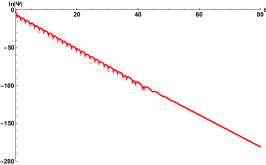
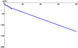
Figure 1: The scalar field profile of in the charged BTZ black hole with $k=3r_{h}=3$, $\mathcal{Q}=0.4$ (left), $\mathcal{Q}=0.5$ (center) and $\mathcal{Q}=0.6$ (right).

The existence of a purely imaginary modes controlling the field evolution is also observed in the non-linear theory with its perturbations. In Aragón et al. (2021) the authors consider a non-linear Maxwell Lagrangean $(F_{\mu\nu}F^{\mu\nu})^{3/4}$ with the correspondent BTZ-like charged black hole. Up to intermediate black hole charges the scalar field evolution ($k>0$) is dominated by oscillatory modes, being the purely imaginary the lowest lying for higher charges.

As a last comment, we point up the role of the cosmological constant in the quasinormal frequencies. Considering the metric (1), if we transform the $R$ coordinate according to (2) and the time coordinate as $\tau\rightarrow L^{-1}t$, the scalar motion equation remains the same as that of (7). Consequently, the quasinormal frequency is impacted by a factor $L$. That represents finally a rescaling of type $\tilde{\omega}\rightarrow L\omega$ in the modes.

V Discussion

In this work we studied the scalar perturbation of the charged BTZ black hole. The propagation of the scalar field was considered with two different methods - characteristic integration and Frobenius - and the quasinormal modes obtained presenting a very good convergence. The frequencies calculated in the paper exibhit a few interesting features.

First, the geometry was not destabilized in all field profiles calculated in our extensive search through characteristic evolution: the stability of the black hole against scalar field perturbation holds.

The modes offer two interesting scalings, the usual one proportional to $r_{h}$ and the other - far from maximum charge values - with the Hawking temperature $\omega\propto T_{H}$ substantiating the interpretation of $\Im(\omega)$ as the inverse of the time for thermal equilibrium in CFT Horowitz and Hubeny (2000).

For higher values of angular momenta, we verify the presence of two families of frequencies fighting to take control of the field evolution. An oscillatory family takes control for small charges whereas a purely imaginary field dominates for higher charges (both families compete in intermediate values, being present in every scenario). By inspecting the BTZ chargeless limit, the oscillatory family is the same present for the special case of $k=0$ but in such, specially represented by purely imaginary evolutions (although further investigation is necessary on the subject).

Further lines of investigation for future works include the study of the superradiant phenomena González et al. (2021); Ortí z (2012); Ho and Kang (1998); Dappiaggi et al. (2018) in the same black hole (that we address in a follow up article) and in charged rotating BTZ black holes (as recently done in Konewko and Winstanley (2023) but with an investigation of the modes). Also valuable is the study of the propagation of another probe fields that could impact the geometry differently.

VI Acknowledgments

The authors acknowledge Jefferson E. E. Portela for critical reading of the manuscript.

Appendix A Tortoise coordinate integration

The tortoise coordinate is defined via lapse function as

$$r_{*}=\int\frac{1}{f}dr,$$ (22)

which is not analytical. In order to implement the integration, we solved the above operator in two stages.

Firstly we define the near-horizon (nh) coordinate $\varepsilon$ as

$$r=r_{h}(1+\varepsilon)\hskip 14.22636pt\rightarrow\hskip 14.22636pt\varepsilon=\frac{r-r_{h}}{r_{h}}.$$ (23)

In such case (22) turns to the form

$$r_{*}^{(nh)}=\int\frac{r_{h}}{\varepsilon^{2}(r_{h}^{2})+\varepsilon(2r_{h})-Q^{2}\ln(1+\varepsilon)}d\varepsilon=\int\frac{r_{h}}{\sum(B_{n}+A_{n})\varepsilon^{n}}d\varepsilon=\int\frac{r_{h}}{\sum b_{n}\varepsilon^{n}}d\varepsilon$$

(24)

in which

$$B_{1}=2r_{h},\hskip 14.22636ptB_{2}=r_{h}^{2},\hskip 14.22636ptB_{n>2}=0,\hskip 14.22636ptA_{n}=Q^{2}\frac{(-1)^{n}}{n}.$$ (25)

Now, with the new expansion,

$$\frac{1}{\sum b_{n}\varepsilon^{n}}=\sum a_{n}\varepsilon^{n-1}$$ (26)

we obtain

$$r_{*}^{(nh)}=r_{h}\left(a_{0}\ln(\varepsilon)+\sum_{n=1}^{N}a_{n}\frac{\varepsilon^{n}}{n}\right),\hskip 19.91684pta_{n}=-\frac{1}{b_{1}}\sum_{j=0}^{n-1}b_{n-j+1}a_{j}$$ (27)

in which $a_{0}=b_{1}^{-1}$. Such technique circumvents integrability issues for $r_{*}$ near $r_{h}$ since it may not be analytically determined, but taken as an approximation by truncating the series.

In the second approximation we expand the tortoise function (22) in the asymptotic region of the AdS spacetime $(ni)$,

$$r_{*}^{(ni)}=\int\sum_{i=0}^{N}\sum_{j=0}^{i}\frac{\mathrm{C}_{i}^{j}M^{i-j}Q^{2j}\ln^{j}(r)}{r^{2i+2}}dr$$ (28)

and

$$r_{*}^{(ni)}=-\sum_{i=0}^{N}\sum_{j=0}^{i}(1+2i)^{-1-j}\mathrm{C}_{i}^{j}M^{i-j}Q^{2j}\Gamma[1+j,(1+2i)\ln(r)].$$ (29)

The convergence of (27) is limited by the maximum value of $r\lesssim 2r_{h}$, while the convergence of (29) is limited by a minimum value $r\gtrsim r_{h}$. Computationally both approximations fail before those points such that the match between the functions is dictated by the chosen charge: the higher the charge the smaller the convergence of both series.

Unfortunately this fact prevents the possibility of investigation of geometries with maximum charge and proximal values $Q\lesssim Q_{max}$.

Appendix B QNM’s compared with different methods

In table 3 we compare the quasinormal modes calculated with different methods, characteristic integration (CI) and Frobenius with the Horowitz-Hubeny (HH) scheme Horowitz and Hubeny (2000) truncated at $N=45$ terms. While the Frobenius method converges in a very short time (a few seconds to a few minutes), the matrix of the tortoise coordinate necessary for the CI method is very time consuming: for higher values of charge a complete calculation can endure a few days. We recall that the convergence in the HH method is limited by $Q\leq r_{h}$, i. e. $\mathcal{Q}\leq 0.5$, while in the CI we have no such limit. (In practice though, it is not possible to go beyond $\mathcal{Q}\sim 0.9$ since the computational time increases exponentially near $\mathcal{Q}=1$).

Table 3: Comparison of quasinormal modes ($k=0$) obtained with different numerics (in the table, $-\Im(\omega)$). All frequencies are purely imaginary and stable.

$\mathcal{Q}$	$r_{h}=1$		$r_{h}=10$		$r_{h}=100$
	CI	HH	CI	HH	CI	HH
0	1.99558	2.00066	19.9529	20.0057	199.509	200.057
0.1	1.44617	1.44630	14.4615	14.4630	144.615	144.630
0.2	1.17840	1.17847	11.7839	11.7847	117.840	117.847
0.3	0.96541	0.96546	9.65401	9.6545	96.5430	96.545
0.4	0.78290	0.78292	7.82894	7.8292	78.2983	78.292
0.5	0.62109	0.62110	6.21092	6.2110	62.1365	62.110

References

- Banados et al. (1992) M. Banados, C. Teitelboim, and J. Zanelli, Phys. Rev. Lett. 69, 1849 (1992), arXiv:hep-th/9204099 .
- Jackiw (1985) R. Jackiw, Nuclear Physics B 252, 343 (1985).
- Mann (1992) R. B. Mann, General Relativity and Gravitation 24, 433 (1992).
- Podolský and Papajčík (2022) J. Podolský and M. Papajčík, Physical Review D 105 (2022), 10.1103/physrevd.105.064004.
- Note (1) In the absence of mass a recent work correlated the spacetime with properties of the graphene Iorio (2022).
- Carlip (1995) S. Carlip, Classical and Quantum Gravity 12, 2853 (1995).
- Martínez et al. (2000) C. Martínez, C. Teitelboim, and J. Zanelli, Physical Review D 61 (2000), 10.1103/physrevd.61.104013.
- Song et al. (2018) Y. Song, H. Tang, D.-C. Zou, C.-Y. Sun, and R.-H. Yue, Chinese Physics B 27, 020401 (2018).
- Düztaş et al. (2020) K. Düztaş , M. Jamil, S. Shaymatov, and B. Ahmedov, Classical and Quantum Gravity 37, 175005 (2020).
- Maity et al. (2010) D. Maity, S. Sarkar, B. Sathiapalan, R. Shankar, and N. Sircar, Nuclear Physics B 839, 526 (2010).
- Li and Yang (2007) H.-L. Li and S.-Z. Yang, Europhysics Letters 79, 20001 (2007).
- Jiang et al. (2007) Q.-Q. Jiang, S.-Q. Wu, and X. Cai, Physics Letters B 651, 58 (2007).
- Ejaz et al. (2013) A. Ejaz, H. Gohar, H. Lin, K. Saifullah, and S.-T. Yau, Physics Letters B 726, 827 (2013).
- Hortaçsu et al. (2003) M. Hortaçsu, H. T. Özçelik, and B. Yapışkan, General Relativity and Gravitation 35, 1209 (2003).
- Soroushfar et al. (2016) S. Soroushfar, R. Saffari, and A. Jafari, Physical Review D 93 (2016), 10.1103/physrevd.93.104037.
- Sharif and Javed (2020) M. Sharif and F. Javed, Modern Physics Letters A 35, 1950350 (2020).
- Astorino (2011) M. Astorino, Journal of High Energy Physics 2011 (2011), 10.1007/jhep01(2011)114.
- Mazharimousavi et al. (2012) S. H. Mazharimousavi, M. Halilsoy, and T. Tahamtan, “Revisiting the charged btz metric in nonlinear electrodynamics,” (2012).
- Bueno et al. (2021) P. Bueno, P. A. Cano, J. Moreno, and G. van der Velde, Physical Review D 104 (2021), 10.1103/physrevd.104.l021501.
- González et al. (2021) P. González, Á. Rincón, J. Saavedra, and Y. Vásquez, Physical Review D 104 (2021), 10.1103/physrevd.104.084047.
- Aragón et al. (2021) A. Aragón, P. A. González, J. Saavedra, and Y. Vásquez, General Relativity and Gravitation 53 (2021), 10.1007/s10714-021-02864-6.
- (22) In Preparation.
- Birmingham et al. (2002) D. Birmingham, I. Sachs, and S. N. Solodukhin, Physical Review Letters 88 (2002), 10.1103/physrevlett.88.151301.
- Hartnoll et al. (2008) S. A. Hartnoll, C. P. Herzog, and G. T. Horowitz, Journal of High Energy Physics 2008, 015 (2008).
- Chen et al. (2012) S.-B. Chen, Q.-Y. Pan, and J.-L. Jing, Chinese Physics B 21, 040403 (2012).
- Cuadros-Melgar et al. (2022) B. Cuadros-Melgar, R. Fontana, and J. de Oliveira, Physical Review D 106 (2022), 10.1103/physrevd.106.124007.
- de Oliveira and Fontana (2018) J. de Oliveira and R. Fontana, Physical Review D 98 (2018), 10.1103/physrevd.98.044005.
- Cadoni and Monni (2009) M. Cadoni and C. Monni, Physical Review D 80 (2009), 10.1103/physrevd.80.024034.
- Note (2) Those are conventionally defined as and in which is the customary tortoise radial coordinate.
- Gundlach et al. (1994) C. Gundlach, R. H. Price, and J. Pullin, Physical Review D 49, 883 (1994).
- Note (3) A detailed description can be found in Konoplya and Zhidenko (2011).
- Horowitz and Hubeny (2000) G. T. Horowitz and V. E. Hubeny, Phys. Rev. D 62, 024027 (2000), arXiv:hep-th/9909056 .
- Cardoso and Lemos (2001) V. Cardoso and J. P. S. Lemos, Physical Review D 63 (2001), 10.1103/physrevd.63.124015.
- Wang et al. (2004) B. Wang, C.-Y. Lin, and C. Molina, Physical Review D 70 (2004), 10.1103/physrevd.70.064025.
- Molina et al. (2004) C. Molina, D. Giugno, E. Abdalla, and A. Saa, Physical Review D 69 (2004), 10.1103/physrevd.69.104013.
- Note (4) In the Reissner-Nordström black hole such variation is even smaller Konoplya (2002).
- Gwak and Lee (2016) B. Gwak and B.-H. Lee, Physics Letters B 755, 324 (2016).
- Destounis et al. (2020) K. Destounis, R. D. Fontana, and F. C. Mena, Physical Review D 102 (2020), 10.1103/physrevd.102.044005.
- Fontana et al. (2021) R. Fontana, P. González, E. Papantonopoulos, and Y. Vásquez, Physical Review D 103 (2021), 10.1103/physrevd.103.064005.
- Cardoso et al. (2018) V. Cardoso, J. L. Costa, K. Destounis, P. Hintz, and A. Jansen, Physical Review Letters 120 (2018), 10.1103/physrevlett.120.031103.
- Ortí z (2012) L. Ortí z, Physical Review D 86 (2012), 10.1103/physrevd.86.047703.
- Ho and Kang (1998) J. Ho and G. Kang, Physics Letters B 445, 27 (1998).
- Dappiaggi et al. (2018) C. Dappiaggi, H. R. Ferreira, and C. A. Herdeiro, Physics Letters B 778, 146 (2018).
- Konewko and Winstanley (2023) S. Konewko and E. Winstanley, “Charge superradiance on charged btz black holes,” (2023).
- Iorio (2022) A. Iorio, (2022), 10.48550/ARXIV.2212.00106.
- Konoplya and Zhidenko (2011) R. Konoplya and A. Zhidenko, Rev. Mod. Phys. 83, 793 (2011), arXiv:1102.4014 [gr-qc] .
- Konoplya (2002) R. A. Konoplya, Physical Review D 66 (2002), 10.1103/physrevd.66.084007.