CPMA: An Efficient Batch-Parallel Compressed Set Without Pointers

Abstract.

This paper introduces the batch-parallel Compressed
Packed Memory Array (CPMA), a compressed, dynamic, ordered set data structure based on the Packed Memory Array (PMA). Traditionally, batch-parallel sets are built on pointer-based data structures such as trees because pointer-based structures enable fast parallel unions via pointer manipulation. When compared with cache-optimized trees, PMAs were slower to update but faster to scan.

The batch-parallel CPMA overcomes this tradeoff between updates and scans by optimizing for cache-friendliness. On average, the CPMA achieves $3\times$ faster batch-insert throughput and $4\times$ faster range-query throughput compared with compressed PaC-trees, a state-of-the-art batch-parallel set library based on cache-optimized trees.

We further evaluate the CPMA compared with compressed PaC-trees and Aspen, a state-of-the-art system, on a real-world application of dynamic-graph processing. The CPMA is on average $1.2\times$ faster on a suite of graph algorithms and $2\times$ faster on batch inserts when compared with compressed PaC-trees. Furthermore, the CPMA is on average $1.3\times$ faster on graph algorithms and $2\times$ faster on batch inserts compared with Aspen.

1. Introduction

The dynamic ordered set data type (also called a key store) is one of the most fundamental collection types and appears in many programming languages as either a built-in basic type or in standard libraries (Blelloch et al., 2016; Sun et al., 2018; Dhulipala et al., 2022). Ordered sets enable efficient scan-based operations (i.e., operations that use ordered iteration) such as range queries and maps. This paper focuses on dynamic ordered sets which also support updates (i.e., inserts and deletes).

Due to their role in large-scale data processing, dynamic ordered sets have been targeted for efficient batch-parallel implementations (Frias and Singler, 2007; Barbuzzi et al., 2010; Dhulipala et al., 2022, 2019; Sun et al., 2018; Erb et al., 2014; Tseng et al., 2019). Since point operations (e.g., single-element insertion) are often not worth parallelizing due to their sublinear complexity, modern libraries parallelize batch updates that insert or delete multiple elements. Direct support for batch updates simplifies update parallelism and reduces the overall work of updates by sharing work between updates.

Existing set implementations demonstrate the importance of optimizing for the memory subsystem to achieve high performance. Almost all fast batch-parallel set implementations are built on pointer-based data structures (e.g., trees) (Dhulipala et al., 2022, 2019; Blelloch et al., 2016; Frias and Singler, 2007; Barbuzzi et al., 2010; Sun et al., 2018; Erb et al., 2014; Tseng et al., 2019). Unfortunately, the main bottleneck in the scalability of these sets is memory bandwidth limitations due to pointer chasing (Blelloch et al., 2016; Frias and Singler, 2007). Dhulipala et al. (Dhulipala et al., 2019, 2022) mitigated these issues in trees by improving spatial locality via blocking and compression.

Even with these improvements, cache-optimized trees inherently leave performance on the table because the random memory accesses from following pointers are slower than contiguous memory accesses (Bender et al., 2019; Pandey et al., 2021; Wheatman and Xu, 2021). In theory, cache-friendly trees such as B-trees (Bayer and McCreight, 1972) are asymptotically optimal in the classical external-memory model (Aggarwal and Vitter, 1988) for both updates and scans. Empirically, array-based data structures support scans over $2\times$ faster than tree-based data structures due to prefetching and the cost of pointer chasing (Pandey et al., 2021; Wheatman et al., 2023a).

Exploiting sequential access with PMAs

This paper introduces a work-efficient batch-parallel Compressed
Packed Memory Array (CPMA) based on the Packed Memory Array (PMA) (Itai et al., 1981; Bender et al., 2000, 2005), a dynamic array-based data structure optimized for cache-friendliness (i.e., spatial locality). The PMA appears in domains such as graph processing (Sha et al., 2017a; Wheatman and Xu, 2018; De Leo and Boncz, 2019a; Wheatman and Xu, 2021; De Leo and Boncz, 2021; Pandey et al., 2021; Wheatman and Burns, 2021), particle simulations (Durand et al., 2012), and computer graphics (Toss et al., 2018).

Existing PMAs suffer from low update throughput compared to batch-parallel trees because they lack direct algorithmic support for parallel batch updates (Wheatman and Xu, 2021). At a high level, batch-update algorithms can be implemented with unions/differences (Blelloch et al., 2016). Previous work (De Leo and Boncz, 2019b) introduced a serial batch-update algorithm for PMAs based on local merges but stopped short of parallelization.

Supporting theoretically and practically efficient parallel unions in a PMA requires novel algorithmic development because existing parallel batch-update algorithms rely heavily on pointer adjustments, which do not easily translate to contiguous memory layouts.

As an additional optimization, this paper adds compression to PMAs. Previous work on compressed blocked trees (Dhulipala et al., 2022, 2019) demonstrates the potential for compression to alleviate memory bandwidth limitations by reducing the number of bytes transferred. This paper applies the same techniques to PMAs.

Figure 1. Insert throughput as a function of batch size.

Figure 2. Range query throughput as a function of range size.

Results summary

The CPMA’s cache-friendliness translates into performance: the CPMA overcomes the traditional tradeoff between updates and queries in trees and PMAs. Figures 1 and 2 demonstrate that the CPMA achieves on average $3\times$ faster batch-insert throughput and $4\times$ faster range-query throughput compared to Parallel Compressed trees (PaC-trees) (Dhulipala et al., 2022). PaC-trees are a state-of-the-art batch-parallel set implementation based on cache-optimized blocked trees. We also found that the uncompressed PMA achieves on average $1.5\times$ faster batch-insert throughput and $20\times$ faster range-query throughput when compared to P-trees (Sun et al., 2018) (PAM), an efficient batch-parallel set implementation based on binary trees. We compare the PMA with P-trees because they are both uncompressed. Finally, CPMAs use similar space to compressed PaC-trees but at least $2\times$ less space than uncompressed PMAs. Furthermore, PMAs use about $3\times$ less space than P-trees.

To understand the improved locality of the PMA compared to PaC-trees, we measured the number of cache misses during batch inserts in both. The PMA incurs at least $3\times$ fewer cache misses when compared to PaC-trees because the PMA takes advantage of contiguous memory access as can be seen in Table 1.

Furthermore, to demonstrate the applicability of the CPMA, we built F-Graph , a dynamic-graph-processing system built on the CPMA because PMAs have been used extensively in graph processing (Sha et al., 2017a; Wheatman and Xu, 2018; De Leo and Boncz, 2019a; Wheatman and Xu, 2021; De Leo and Boncz, 2021; Pandey et al., 2021; Wheatman and Burns, 2021). F-Graph is on average $1.2\times$ faster on a suite of graph algorithms and $2\times$ faster on batch updates compared to C-PaC, a dynamic-graph-processing framework based on compressed PaC-trees. F-Graph uses marginally less space to store the graphs when compared to C-PaC. We also evaluate Aspen (Dhulipala et al., 2019), a state-of-the-art dynamic-graph-processing framework based on compressed blocked trees. We find that F-Graph is on average $1.3\times$ faster on graph algorithms, $2\times$ faster on batch updates, and uses about $0.6\times$ the space when compared to Aspen.

Workload	U-PaC (Dhulipala et al., 2022)	C-PaC (Dhulipala et al., 2022)	PMA	CPMA
L1 misses	3.1E9	2.2E9	8.9E8	7.0E8
L3 misses	3.1E8	7.6E7	9.6E7	1.1E7

Table 1. Cache misses incurred during batch inserts.

Contributions

• The design and analysis of a theoretically efficient parallel batch-update algorithm for PMAs (and for CPMAs).

• An implementation of the PMA and CPMA with the parallel batch-update algorithm in C++.

• An evaluation of the PMA/CPMA with PaC-trees and P-trees.

• An evaluation of F-Graph, a dynamic-graph-processing system based on the CPMA, compared to C-PaC and Aspen.

	Work			Span
Operation	CPMA (this work)	Compressed PaC-tree  (Dhulipala et al., 2022)		CPMA (this work)	Compressed PaC-tree (Dhulipala et al., 2022)
Insert/delete	$O((\log^{2}(n))/B+\log(n))^{\dagger}$	$O(\log(n)+P)$		$O(\log(n))$	$O(\log(n)+P/B)$
Batch insert/delete	$O(k((\log^{2}(n))/B+\log(n)))$$\dagger$	$O(k\log(n/Pk))^{\dagger}$		$O(\log(k)+\log^{2}(n))$	$O(\log(n/P)\log k+P/B)$
Search	$O(\log(n))$	$O(\log(n)+P)$		$O(\log(n))$	$O(\log(n)+P/B)$
Range query	$O(\log(n)+r/B)$	$O(\log(n)+(P+r)/B)$		$O(\log(n))$	$O(\log(n)+P/B)$

Table 2. Asymptotic bounds for operations in a CPMA and compressed PaC-tree. We use $B$ to denote the cache-line size, $k$ to denote the size of the batch, $r$ to denote the number of elements returned by the range query, and $P$ to denote the user-specified tree node block size in the PaC-tree (called $B$ in (Dhulipala et al., 2022)). Bounds with ^$\dagger$ are amortized. All bounds are $\Omega(1)$.

2. Related work

This section describes how this work relates to prior work in parallel data structures. Specifically, it discusses concurrent versus batch-parallel data structures and their use cases.

There is extensive work on concurrent data structures such as trees (Aksenov et al., 2017; Arbel-Raviv et al., 2018; Braginsky and Petrank, 2012; Bronson et al., 2010; Mao et al., 2012; Ellen et al., 2010; Kung and Lehman, 1980; Natarajan and Mittal, 2014), skip lists (Herlihy et al., 2006; Pugh, 1998), and PMAs (Wheatman and Xu, 2021). Concurrent data structures are mostly orthogonal to this paper, which focuses on batch-parallel data structures. Existing concurrent trees typically support mostly point operations (i.e., linearizable inserts/deletes and finds), whereas the CPMA in this paper also supports range queries and maps (and associated operations such as filter and reduce). Some recent work studies range queries in concurrent trees (Basin et al., 2020; Fatourou et al., 2019). On the other hand, concurrent trees support asynchronous updates, which are more general than batch updates because batch updates require a single writer. Therefore, fairly comparing concurrent and batch-parallel data structures on update throughput is challenging as their update functionalities are different.

The PAM paper (Sun et al., 2018) demonstrated that batch-parallel binary trees can achieve orders of magnitude higher insertion throughput compared to concurrent cache-optimized trees (Mao et al., 2012; Wang et al., 2018; Zhang et al., 2016).

Batch-parallel and concurrent data structures are suited for different use cases. For example, batch-parallel data structures have recently become popular for both practical (Ediger et al., 2012; Kyrola et al., 2012; Macko et al., 2015; Dhulipala et al., 2019) and theoretical (Acar et al., 2019; Nowicki and Onak, 2021; Dhulipala et al., 2020, 2021; Ferragina and Luccio, 1994; Tseng et al., 2019) dynamic-graph algorithms and containers. They are well-suited for applications with a large number of requests in a short time, such as stream processing or loop join (Kim et al., 2010). In contrast, concurrent data structures have been used extensively in key-value stores for online transaction processing applications that emphasize point operations such as put and get (Cooper et al., 2010).

3. Packed Memory Array

This section reviews the Packed Memory Array (Bender et al., 2000; Itai et al., 1981) (PMA) data structure to understand the improvements in later sections. First, it introduces the theoretical models used to analyze the PMA. It then describes the PMA’s structure and supported operations. Finally, it details how to perform point updates in a PMA, which forms the basis for the batch-update algorithm in Section 4.

Analysis method

Table 2 summarizes the bounds for key parallel operations in the CPMA and compressed PaC-tree in the work-span model (Cormen et al., 2009, Chapter 27) and the external-memory model (Aggarwal and Vitter, 1988). The work is the total time to execute the entire algorithm in serial. The span is the longest serial chain of dependencies in the computation. In the work-span model with binary forking, a parallel for loop with $k$ iterations with $O(1)$ work per iteration has $O(k)$ work and $O(\log(k))$ span.

The external-memory model introduces the cache-line-size parameter $B$ and measures algorithm cost in terms of cache-line transfers.

Design and operations

The PMA maintains elements in sorted order in an array with (a constant factor of) empty spaces between its elements. Specifically, a PMA with $n$ elements uses $N=\Theta(n)$ cells. The empty cells enable fast updates by reducing the amount of data movement necessary to maintain the elements in order. The primary feature of a PMA is that it stores data in contiguous memory, which enables fast cache-efficient iteration through the elements.

A PMA exposes four operations:

• insert(x): inserts element x into the PMA.

• delete(x): deletes element x from the PMA, if it exists.

• search(x): returns a pointer to the smallest element that is at least x in the PMA.

• range_map(start, end, f): applies the function f to all elements in the range [start, end).

In this paper, we use the terms “range map” and “range query” interchangeably. Range queries can be implemented with the more general range map, but we use the more popular term “range query.”

The PMA supports point queries (search) in $O(\log(n))$ cache-line transfers and updates in $O((\log^{2}(n))/B+\log(n))$ (amortized and worst-case) cache-line transfers (Bender et al., 2017, 2000, 2005; Willard, 1982, 1986, 1992). The PMA supports efficient iteration of the elements in sorted order, enabling fast scans and range queries. Specifically, the PMA supports the range_map operation on $k$ elements in $O(\log(n)+k/B)$ transfers. It implements range_map with a search for the first element in the range, then a scan until the end of the range. PMAs are asymptotically worse than PaC-trees for all inserts/deletes and match them for search and range queries (Table 2).

The PMA defines an implicit binary tree with leaves of size $\Theta(\log(N))$ cells. That is, the implicit tree has $\Theta(N/\log(N))$ leaves and height $\Theta(\log(N/\log(N)))$. Every node in the PMA tree has a corresponding region of cells. Each leaf
$i\in\{0,\ldots,N/\log(N)-1\}$ has the region $[i\log(N),(i+1)\log(N))$, and each internal node’s region encompasses all of the regions of its descendants. The density of a region in the PMA is the fraction of occupied cells in that region.

Each node of the PMA tree has an upper density bound that determines the allowed number of occupied cells in that node. If an insert causes a node’s density to exceed its upper density bound, the PMA enforces the density bound by redistributing elements with that node’s sibling, equalizing the densities between them. The density bound of a node depends on its height.

Updating a PMA

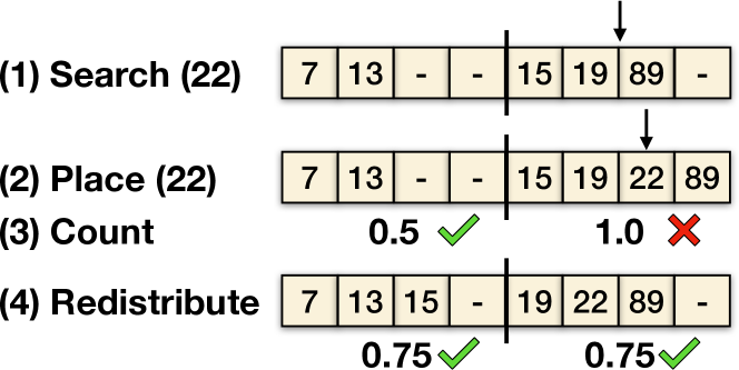
Figure 3. Example of an insertion in a PMA with leaf density bound of 0.9 and leaf size of 4.

A PMA maintains spaces between elements for efficient updates. Since deletions are symmetric to insertions, we omit the discussion of deletes.

As shown in Figure 3, the four main steps in a PMA insertion are as follows:

1. Search for the location that the element should be inserted into to maintain global sorted order.

2. Place the element at that location, potentially shifting some elements to make room.

3. If the leaf that was inserted into violates its density bound, count the density of nodes in the PMA to find a sibling to redistribute into.

4. If necessary, redistribute elements to maintain the correct distribution of empty spaces in the PMA.

The four steps of a PMA insertion use the implicit tree to determine which leaf to modify and which node to redistribute, if any. Steps (1) and (2) take $O(\log(n))$ cache-line transfers. Counting and redistributing elements (steps (3) and (4)) take $O((\log^{2}(n))/B)$ (amortized and worst-case) cache-line transfers (Bender et al., 2017, 2000, 2005; Willard, 1982, 1986, 1992).

Resizing a PMA

If the root-to-leaf traversal after an insert reaches the root and finds that its density bound has been violated, the entire PMA is copied to a larger array and the elements are distributed equally amongst the leaves of the new PMA.

4. Parallel Batch Updates in a PMA

Batching updates in a PMA improves throughput by sharing work between updates and simplifying parallelization. This section describes how to apply batch inserts in a PMA (batch deletes are symmetric).

We present a work-efficient parallel batch-insert algorithm for PMAs. A work-efficient parallel algorithm performs no more than a constant factor of extra operations than the serial algorithm for the same problem. Serially inserting $k$ elements into a PMA with $n$ elements takes $O(k(\log(n)+(\log^{2}(n))/B))$ cache-line transfers. Unfortunately, a naive algorithm that parallelizes over the inserts is not work-efficient because it may recount densities to determine which regions to redistribute. Supporting work-efficient batch inserts requires careful algorithm design to avoid redundant work. Finally, we conclude the section with a microbenchmark that demonstrates the serial and parallel scalability of batch inserts in PMAs.

The batch-insert problem for PMAs takes as input a PMA with $n$ elements and a batch with $k$ sorted elements to insert. An unsorted batch can be converted into a sorted batch in $O(k\log(k))$ work.

The optimal strategy for applying a batch of updates depends on the size of the batch. At one extreme, if $k$ is small (e.g., $k<100$), the overheads from the batch-update algorithm outweigh the benefits, so point updates are more efficient than batch updates. At the other extreme, if $k$ is large (e.g., $k\geq n/10$), the optimal algorithm is to rebuild the entire data structure with a linear two-finger merge . The batch-insert algorithm for PMAs performs local merges to address the intermediate case between these two extremes.

The parallel batch-insert algorithm for PMAs applies a batch of updates efficiently in the case where neither point insertions nor a complete merge are the best options. Therefore, we focus on the case where $\omega(1)=k=o(n)$.

The batch-insert algorithm consists of three phases: (1) a batch-merge phase, (2) a counting phase, and (3) a redistribute phase. The phases proceed in serial, but each phase is parallelized internally. The phases adapt the steps of a PMA insertion described in Section 3 to the batch setting. The batch-merge phase combines the search and place steps, and the counting and redistribute phases generalize their counterparts from point inserts.

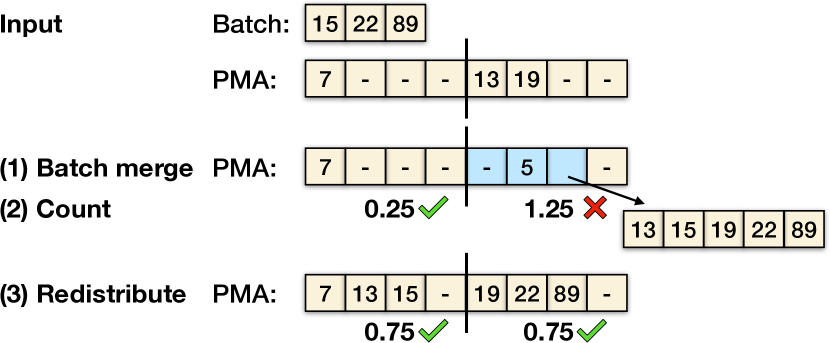
Figure 4. Example of batch insertion in a PMA with leaf density bound of 0.9 and leaf size of 4. After the merge, there are more elements in the second leaf than the leaf size, so the number of elements is stored in the leaf, and the elements are stored out-of-place until the redistribute.

At a high level, the parallel batch-merge phase divides the PMA and the batch recursively into independent sections and operates independently on those sections. Each recursive step first merges elements from the batch into one leaf of the PMA, and then recurses down on the remaining left and right portions of the batch. This recursive merge phase is inspired by recursive join-based algorithms in batch-parallel trees (Adams, 1992, 1993; Dhulipala et al., 2022, 2019; Blelloch et al., 2016; Sun et al., 2018). Existing join algorithms for tree layouts rely on pointer adjustments which do not easily translate into array layouts.

At each step of the recursion, we perform a PMA search for the midpoint (median) of the current batch and merge the relevant elements from the batch destined for that leaf into the target leaf. Finding the bounds in the batch of all elements in that leaf takes two searches (one backwards and one forwards). Once the endpoints have been found, we fork the merge of all relevant elements from the current batch into the target leaf. If the number of elements destined for a leaf is sufficiently large, we use a parallel merge algorithm with load-balancing guarantees to achieve parallelism (Akl and Santoro, 1987). Finally, we recurse on the remaining left and right sides of the batch in parallel.

Lemma 1.

Given a batch of $\;k$ sorted elements, the work of the batch-merge phase is $O(k\log(n))$, and the span is
$O(\log(k)\log(n))$.

Proof.

The height of the recursion is $O(\log(k))$, and each search in the PMA takes $O(\log(n))$ work. Finding the first and last element in the batch destined for the leaf takes $O(\log(k))$ work with exponential searches, which is smaller than
$O(\log(n))$. Therefore, the work and span of finding the bounds for the recursion is $O(\log(k)\log(n))$.

In the worst case for the work, each element in the batch could be destined for a different leaf, so the total work of merging $k$ elements into $k$ leaves is $O(k\log(n))$, which is asymptotically larger than the work to perform the recursion.

The worst-case span for any one of the merges is $O(\log(k))$, so the total worst-case span of all the merges is $O(\log^{2}(k))$, which is less than $O(\log(k)\log(n))$. ∎

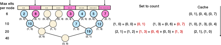
Figure 5. An example of the work-efficient counting algorithm for batch updates. The blocks at the top represent the PMA leaves and the dots represent elements in the PMA. The pink blocks with arrows represent leaves that were touched during a batch update. The tree below the PMA is the implicit PMA tree of nodes labeled with a tuple of (height, index) (indices are assigned left to right). The blue solid circles represent PMA nodes that must be counted because their sibling or child violated its density. The tan dotted circles represent PMA nodes that did not need to be counted.

When merging elements from the batch into a leaf, the target leaf may overflow because it does not have enough space to hold all the elements destined for it. To resolve this issue, the batch merge copies all elements into separate memory and keeps the size of the extra memory as well as a pointer to it in the leaf. This extra data is then cleaned up after the merge during the redistribution phase.  Figure 4 illustrates a batch merge, leaf overflow, and subsequent redistribution.

During the recursive batch merge, we keep track of all modified PMA leaves in a thread-safe set for use in the counting and redistribution phases.

Counting phase

After merging all elements into the PMA, the batch insert algorithm performs a counting phase where it finds the PMA nodes that violate their density bounds for later redistribution. The $O(\log^{2}(n)/B)$ work bound for point insertions in the PMA comes from amortized analysis of the counting and redistribution phase (Itai et al., 1981), so efficiently counting and redistributing in the batch-parallel setting is critical to achieving work-efficiency. To understand how to avoid redundant work, we start with a presentation of an efficient serial algorithm and describe how simply parallelizing this algorithm can lead to extra work. We then present our work-efficient parallel algorithm.

An efficient serial batch algorithm must count each required cell exactly once. The algorithm starts with the set of leaves that were touched in the batch-merge phase. The ancestors of these leaves in the implicit PMA tree may need to be redistributed. The serial algorithm checks every leaf in turn. If a leaf violates its density bound, the algorithm then walks up the implicit PMA tree from that leaf until it finds a node that respects its density bound. Finding the density of a node involves counting all of its descendants. By caching every result and checking the cached results before counting, the serial algorithm counts every required cell exactly once.

Unfortunately, simply parallelizing this serial algorithm over the leaves is not work-efficient because the algorithm may recount PMA nodes whose densities have not been cached yet. Therefore, the parallel algorithm may recount the same region more than a constant number of times if many leaves share the same ancestor to be redistributed.

To resolve this issue, we devise a new work-efficient parallel counting algorithm that counts each required PMA cell exactly once.  Figure 5 presents a worked example of this counting algorithm. The counting algorithm takes as input the leaves that were modified in the batch merge and outputs the set of PMA nodes that need to be redistributed.

This parallel algorithm avoids redundant work by processing the levels serially from the leaves to the root and saving any counts for later lookups by nodes in higher levels. At each level, we maintain a thread-safe set of nodes that need to be counted. This set is initialized with the leaves that were affected by the batch merge. The levels are processed serially, but all nodes at each level are processed in parallel. If any node at some level $i$ exceeds its density bound, the algorithm adds its parent to the set of nodes to be counted at level $i+1$. The algorithm terminates when there are no more nodes to be counted, or it has reached the PMA root.

Lemma 2.

The parallel counting algorithm is work-efficient.

Proof.

The parallel counting algorithm caches results from each counted region as it processes the levels of the PMA tree. Due to the serial iteration of levels, all nodes to be counted at a level are counted in parallel. When a node $x$ needs to be counted, no other node $y$ at that level will need to count any of $x$’s descendants since the set ensures that $x\neq y$. All descendants of $x$ have either already been counted and cached, or will be counted exactly once and cached to avoid recounting. ∎

Lemma 3.

The span of the parallel counting algorithm is $O(\log^{2}(n))$.

Proof.

The counting algorithm serially iterates over at most $O(\log(n))$ levels of the PMA because the height of the PMA tree is bounded by $O(\log(n))$. In the worst case, for each level $i$, the algorithm may have to recurse down $i$ levels to count, so the worst-case span of traversing the PMA tree levels is: $\sum_{i=0}^{\log(n)}i=O(\log^{2}(n))$. The PMA leaves are $O(\log(n))$ cells each, so the total span of counting is $O(\log^{2}(n))$. ∎

Redistribution phase

Once the counting phase has identified the correct regions to redistribute, the PMA redistributes regions by performing two copies of the relevant data. The first copy packs the regions to redistribute from the PMA into a buffer, and the second copy equalizes the densities in the regions to redistribute by spreading the elements evenly from the buffer into the target leaves.

Lemma 4.

Given a batch of $\;k$ sorted elements, the work of the redistribute phase is $O((k\log^{2}(n))/B))$ amortized cache-line transfers, and the worst-case span is $O(\log^{2}(n))$.

Proof.

The work of the redistribute phase is bounded above by the work of the counting phase, because the number of elements that need to be redistributed is at most the number of elements that need to be counted. From Lemma 2, the counting step is work-efficient, so it takes no more than the serial amortized work bound of $O((k\log^{2}(n))/B))$ cache-line transfers.

The span of the redistribute phase is bounded above by $O(\log^{2}(n))$ because there are at most $n$ independent sections to redistribute of size $n$ each. Redistributing each one involves a parallel copy in and out, which has span $O(\log(n))$. ∎

Putting it all together

Analyzing the entire batch-insert algorithm just involves summing the work and span of the merge, counting, and redistribute phases of the batch-insert algorithm.

Theorem 5.

The batch-insert algorithm for PMAs inserts a batch of $\;k$ sorted elements in $O(k(\log(n)+\log^{2}(n)/B))$ amortized work and $O(\log^{2}(n))$ worst-case span.

Batch size	Serial TP	Speedup over serial point	Parallel TP	Speedup over serial batch	Overall speedup
1—10	2.2E6	1.0	1.8E6	0.8	0.8
1E2	1.9E6	0.9	3.0E6	1.6	1.4
1E3	2.0E6	0.9	9.0E6	4.6	4.1
1E4	2.0E6	0.9	2.5E7	12.5	11.6
1E5	2.3E6	1.0	4.1E7	17.8	18.6
1E6	2.9E6	1.3	7.0E7	23.8	32.0
1E7	5.5E6	2.5	1.0E8	18.6	47.1

Table 3. Throughput (TP) of serial and parallel batch insertions in the PMA. We use point insertions for small batches when the batch update algorithm does not provide practical benefits. Overall speedup is the speedup over serial point inserts.

Batch insert microbenchmark

Table 3 reports the throughput of batch inserts as a function of batch size (using the setup described in Section 6). The PMA under test starts with 100 million elements and we add an additional 100 million elements.

On one core, the batch-insert algorithm is up to $3\times$ faster than point inserts when the batch is large. Batch inserts in a PMA save computation over point insertions by reducing the number of searches, the length of each search, and the number of redistributions. The batch algorithm performs only one binary search per updated leaf because the remaining elements in the batch destined for that leaf are merged in directly. Additionally, the searches are smaller because they often search only a subsection of the PMA. Finally, the counting algorithm combines ancestor ranges to redistribute in the PMA, potentially skipping levels of redistribution.

Furthermore,  Table 3 shows that batch inserts in a PMA achieve parallel speedup of up to about $19\times$ on $64$ cores ($128$ threads) as the batch size grows. The main bottleneck in the parallel scalability of batch updates is memory bandwidth. Section 5 mitigates these issues by adding compression to the batch-parallel PMA to reduce data movement.

5. Compressed Packed Memory Array

This section introduces, analyzes, and empirically evaluates the Compressed Packed Memory Array (CPMA). Adding compression does not affect the PMA’s asymptotic bounds. Empirically, the CPMA achieves better parallel scalability than the PMA because the parallel operations are memory-bound, so the CPMA’s smaller size makes better use of memory bandwidth.

Data compression techniques

The CPMA exploits the fact that elements are stored in sorted order in a PMA to apply delta encoding (Smith et al., 1997) to the elements. Delta encoding stores differences (deltas) between sequential elements rather than the full element. Given a sorted array $A$ of $n$ elements, delta encoding results in a new array $A^{\prime}$ such that $A^{\prime}_{0}=A_{0}$ and for all $i=1,2,\ldots,n-1$, $A^{\prime}_{i}=A_{i}-A_{i-1}$.

These deltas can then be stored in byte codes, which store an integer as a series of bytes (Witten et al., 1999; Blandford et al., 2004). Each byte uses one bit as a continue bit, which indicates if the following byte starts a new element or is a continuation of the previous element.

We use delta encoding with byte codes in the CPMA because they are fast to decode and achieve most of the memory savings of shorter codes (Shun et al., 2015; Dhulipala et al., 2019; Blandford et al., 2004).

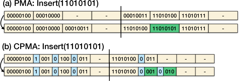
Figure 6. An example of inserting the same element in a PMA and CPMA with the same elements. The density bound in all leaves is 0.9. Here, sizeof(T) is 8 bits, and a byte is 4 bits. The blue bits in the CPMA represent continue bits. The green shaded cells in both the PMA and CPMA contain new data after the insert. The PMA redistributes its elements after the insertion, but the CPMA does not because the insertion did not violate the leaf density bound.

CPMA structure

The CPMA maintains the same implicit binary tree structure as a PMA and compresses the leaves. Just like in the PMA, a CPMA with $n$ elements and $N=\Theta(n)$ cells maintains leaves of size $\Theta(\log(n))$ in order to achieve its asymptotic time bounds. The CPMA applies the packed-left optimization, which packs elements to the left in PMA leaves, for ease of compression (Wheatman and Xu, 2021). Packing the elements to the left does not affect the PMA’s (or CPMA’s) asymptotic bounds because the bounds only depend on the density of the elements in the PMA leaves (Wheatman and Xu, 2021).

A CPMA leaf stores its head, or its first element, uncompressed, and stores subsequent elements compressed with delta encoding and byte codes. That is, in a CPMA with elements of type T, the first sizeof(T) bytes in each leaf contain the uncompressed head. All following cells take 1 byte each rather than sizeof(T) bytes.

The density bounds in a CPMA count byte density rather than element density. The density in a CPMA node is the ratio of the number of filled bytes to the total number of bytes available in the node.

CPMA Operations

The CPMA maintains the same asymptotic bounds as the PMA for point queries (searches) and point updates. Furthermore, compression does not affect concurrency schemes for PMAs (Wheatman and Xu, 2021) or the batch-update algorithm from Section 4.

The PMA’s asymptotic bounds are derived from its implicit tree structure and related density bounds. The main change in the CPMA is the compression of each individual leaf, which does not affect the high-level implicit tree structure.

The uncompressed head allows for efficient searching to find which leaf contains an element. The compressed leaves in the CPMA do not affect the high-level tree structure or searches because each leaf can still be processed independently in $O(\log(n))$ work.

Point queries

A CPMA on $n$ elements supports point queries in $O(\log(n))$ cache-line transfers. There are two steps in a point query in a CPMA: a binary search on leaf heads, and then a pass through the leaf at the end of the binary search to find the closest element. There are $O(n/\log(n))$ leaves, so a binary search takes $O(\log(n))$ cache-line transfers. The leaf heads are stored uncompressed, so there is no additional cost to perform the binary search on leaf heads compared to a search in a PMA. After finding the target leaf, the CPMA performs a search within that leaf. The size of each leaf is bounded by $O(\log(n))$, so it takes $O(\log(n)/B)$ cache-line transfers to search a compressed leaf.

Point updates

A CPMA on $n$ elements supports point updates in $O(\log(n)+(\log^{2}(n))/B)$ cache-line transfers. We will focus on the case of inserts, since deletes are symmetric to inserts. Figure 6 presents a worked example of the same insert in a PMA and a CPMA.

The CPMA follows the same four steps of a PMA point update described in Section 3. We will focus on steps (2)-(4) (place, count, and redistribute), since we already analyzed point queries.

After performing a point query to find the target leaf, the CPMA places an element by adding a delta to the leaf and updating the following delta. Updating the leaf can be done in a single pass, which modifies up to $O(\log(n))$ cells because the size of the leaf is bounded by $O(\log(n))$. The CPMA matches the PMA’s asymptotic bound on the number of cells modified during the place step.

Once the target leaf has been updated, the CPMA traverses up the leaf-to-root path and redistributes any nodes that violate their density bounds just as in a PMA. The amortized insert time bound comes from the checking and maintenance of density bounds, which the CPMA supports in the same asymptotic cache-line transfers as a PMA. Just as in a PMA, counting and redistributing in a CPMA takes cache-line transfers linear in the size of the region.

Parallelizing the CPMA

The compression in the CPMA does not conflict with existing lock-based multiple-writer parallelism for PMAs (Wheatman and Xu, 2021) because the locking scheme depends on the implicit PMA tree structure and locking at a leaf granularity. Furthermore, compression does not affect the theoretical performance of concurrent PMAs because the CPMA also supports single-pass operations within leaves. The CPMA supports multiple readers because reads are non-modifying.

Finally, the batch-update algorithm in the CPMA is identical to the batch-update algorithm for PMAs described in Section 4. The design and analysis of the batch-update algorithm also depends only on single-pass operations on leaves.

Scalability analysis

Figure 7. Scalability of batch inserts in the PMA/CPMA. We use 64 to denote all physical cores and 64h to denote all 128 hyperthreads.

We measure the scalability of both the PMA and CPMA on batch inserts and range queries using the setup described in Section 6. In each experiment, the PMA and CPMA start with 100 million elements. In each batch-insert experiment, we add 100 batches of 1 million elements each. In each range-query experiment, we perform 100,000 range queries in parallel where each query is expected to return about $1.5$ million elements. We measure the effect of core count on performance of the PMA/CPMA. The extended version of the paper contains the raw data.

Figure 7 shows that the CPMA achieves better scalability than the PMA on batch inserts because compression maximizes the CPMA’s usage of available memory bandwidth. The PMA achieves up to $19\times$ speedup and the CPMA achieves up to $43\times$ speedup for batch inserts on $64$ cores ($128$ threads). The CPMA achieves better batch insert throughput compared to the PMA when the number of cores is sufficiently large (at least 16). When the number of cores is too small, the additional computational overhead from compression outweighs the benefits of decreased memory traffic.

Figure 8. Scalability of range queries in the PMA/CPMA. We use 64 to denote all physical cores and 64h to denote all 128 hyperthreads.

Similarly, Figure 8 demonstrates that the PMA achieves about $41\times$ speedup for range queries and the CPMA achieves about $118\times$ speedup for range queries on $64$ cores ($128$ threads). The PMA’s/CPMA’s scalability on range queries is much better than its scalability on updates because the queries proceed in parallel and do not need to coordinate. The PMA’s range query throughput in terms of bytes transferred per second reaches the memory bandwidth on the machine, but its overall range query throughput is limited because of the large size per element. The CPMA alleviates the memory bandwidth issue by decreasing the size per element, enabling it to support more elements processed per byte transferred.

6. Evaluation

To measure the improvements described in Sections 4 and 5, this section evaluates the PMA/CPMA compared to uncompressed/compressed PaC-trees (Dhulipala et al., 2022) and P-trees (Sun et al., 2018) on range queries, batch inserts, and space usage. We use the terms “U-PaC” and “C-PaC” to denote the uncompressed and compressed versions of PaC-trees, respectively, in this section.

This section then evaluates the CPMA, C-PaC, and Aspen (Dhulipala et al., 2019), a state-of-the-art dynamic-graph processing system based on compressed trees, on an application benchmark of dynamic-graph processing because both PMAs and trees appear frequently as dynamic-graph containers (Sha et al., 2017a; Wheatman and Xu, 2018; De Leo and Boncz, 2019a; Wheatman and Xu, 2021; De Leo and Boncz, 2021; Pandey et al., 2021; Dhulipala et al., 2019, 2022; Wheatman and Burns, 2021). We introduce F-Graph, a system for processing dynamic graphs that uses the CPMA as its underlying data structure.

Additional experiments and data tables can be found in an extended version of this paper (Wheatman et al., 2023b).

Microbenchmarks summary

At a high level, the CPMA achieves the best of both worlds in terms of performance. On average, it achieves $4\times$ faster range-query throughput and $3\times$ faster batch-insert throughput when compared to compressed PaC-trees. According to the theoretical prediction in Table 2, PaC-trees asymptotically match or beat CPMAs for all operations. However, in practice, the CPMA supports both fast queries and updates due to its locality. Finally, CPMAs use about the same space as compressed PaC-trees, but they use less than half the space of uncompressed PMAs. When compared with PAM, an uncompressed data structure, the uncompressed PMA achieves $1.5\times$ faster throughput for batch insertions and $20\times$ faster range query throughput.

Graph benchmark summary

For graph workloads, we found that F-Graph is on average $1.2\times$ faster on a suite of graph algorithms, achieves $2\times$ faster throughput for batch updates, and uses marginally less space to store the graphs compared to C-PaC. Furthermore, F-Graph is on average $1.3\times$ faster on graph algorithms, achieves $2\times$ faster throughput for batch updates, and uses $0.6\times$ space to store the graphs compared to Aspen.

Systems setup

We implemented the PMA and CPMA as a C++ library on top of the search-optimized PMA (Wheatman et al., 2023a) and compiled them with clang++-14. To match the parallelization method from the PaC-trees library, we parallelized the PMA/CPMA with the Parlaylib toolkit (Blelloch et al., 2020). The PMA and CPMA are currently implemented as key stores (sets). The code can be found on https://github.com/wheatman/Packed-Memory-Array.git.

Each external library is compiled using the default configuration of g++-11 and Parlaylib (or PBBSlib, a precursor to Parlaylib, for Aspen) for parallelization. They are each implemented in a C++ library. We used the in-place set mode of P-trees and PaC-trees for a fair comparison (although the libraries also support a less efficient functional mode). The PaC-trees library block size is set to the default for sets at 256, which corresponds to a maximum node size of 4108 bytes. To initialize PaC-trees, we used the library-provided recursive build routine, which lays out the tree nodes non-contiguously in memory.

We also tested the Rewired PMA (RMA) (De Leo and Boncz, 2019b) and compiled it with the default provided scripts which used clang++-14. Since the RMA is serial, there is no parallelization framework.

All experiments were run on a 64-core 2-way hyper-threaded Intel^® Xeon^® Platinum 8375C CPU @ 2.90GHz with 256 GB of memory from AWS (Amazon, 2022). Across all the cores, the machine has 3 MiB of L1 cache, 80 MiB of L2 cache, and 108 MiB of L3 cache. All performance results are the average of 10 trials after a single warm up trial.

Evaluation on microbenchmarks

We first evaluate the RMA, P-trees, and PaC-trees compared to the PMA/CPMA on a suite of microbenchmarks.

Experimental setup

We evaluate batch-update throughput first with $40$-bit uniform random numbers. $40$-bit numbers gives a balance between the compression ratio and the number of duplicates. Uniform random is the worst case for compressed data structures because it maximizes the deltas between elements and therefore minimizes the compression ratio. Uniform random is also the worst case for batch inserts because it minimizes the amount of shared work between updates that the algorithm can eliminate. However, uniform random is the best case for redistributes in PMAs/CPMAs.

We also evaluate batch-update throughput by starting with $40$-bit uniform random numbers and then adding elements according to a zipfian distribution. The zipfian distribution generates $34$-bit numbers with skew parameter $\alpha=0.99$ (parameter taken from the YCSB (Cooper et al., 2010)). For additional batch-insert experiments on skewed distributions, we test the data structures on a skewed RMAT distribution (Chakrabarti et al., 2004) in the graph-processing application benchmark at the end of this section.

We measure range-query performance of the data structure when it contains 100 million elements by performing 100,000 range queries in parallel. We varied the size of the range queries across experiments. We measure batch-insert performance, by inserting 100 million elements in batches into a data structure that starts with 100 million elements. We varied the batch size across experiments. If the batch-insert performance was slower than the non-batched insert done in a loop, the non-batched insert number was reported.

To measure the space usage, we vary the number of elements and report the size.

Finally, we evaluate the serial batch-update algorithm from the Rewired PMA (RMA) (De Leo and Boncz, 2019b) with the provided test code and build scripts. For a fair comparison, we ran the batch update algorithm for PMAs from Section 4 on one core.

The RMA’s provided tests use the numbers $[1,2,\ldots,n]$ sampled without replacement where $n$ is the total number of elements after the test. Although this is not exactly the same set as numbers as in our PMA experiments (with uniform random 40-bit numbers), the experiments are equivalent because both data structures are uncompressed, so only the ordering of the numbers matters.

Batch inserts on uniform random inputs

Figure 1 demonstrates that the throughput of parallel batch inserts in the CPMA is on average $3\times$ faster than in compressed PaC-trees. Similarly, parallel batch inserts in the PMA achieve on average $1.5\times$ faster throughput than in P-trees. The PMA’s/CPMA’s cache-friendliness enables it to support faster updates than the theory suggests. As mentioned in Section 3, PMAs (and by extension, CPMAs) support point updates in $O((\log^{2}(n))/B+\log(n))$ work. Trees theoretically dominate PMAs for point updates: balanced binary trees support updates in $O(1+\log(n))$ work (Cormen et al., 2009), and cache-friendly trees such as B-trees (Bayer and McCreight, 1972) support updates in $O(1+\log_{B}(n))$ work. However, in practice, batch updates in a PMA/CPMA are faster than batch updates in trees because the PMA/CPMA takes advantage of contiguous memory access.

Batch size	RMA (De Leo and Boncz, 2019b)	PMA	PMA/RMA
1—1E4	1.7E6	2.2E6	1.3
1E5	2.0E6	2.4E6	1.2
1E6	2.5E6	3.2E6	1.3
1E7	5.4E6	6.5E6	1.2

Table 4. Serial batch insert throughput (inserts per second) of the uncompressed PMA and RMA. We use point insertions for small batches when the batch update algorithm does not provide practical benefits.

Table 4 evaluates the batch-insert algorithm for uncompressed PMAs from Section 4 on one core compared to the existing serial batch-insert algorithm for RMAs, an optimized version of PMAs (De Leo and Boncz, 2019b). On average, the batch-insert algorithm in this paper is about $1.2\times$ faster than the existing batch-insert algorithm for RMAs.

Batch inserts on skewed inputs

Just as in the uniform random case, the CPMA outperforms C-PaC on small batches and is slightly slower on large batches of skewed inserts.

The batch-parallel PMA is well-suited for the case of all insertions targeting the same leaf. In contrast, for non batched PMAs, this is the worst case. The batch-insert PMA mitigates the worst case by (1) sharing the work of searches between inserts, reducing overall work, and (2) skipping levels of redistribution with larger batches, improving overall work and parallelism. Due to these factors, the PMA/CPMA achieves higher throughput on zipfian batch inserts compared to uniform random batch inserts as can be seen in Table 5.

Batch deletes

On average, the PMA performs uniform random batch deletions $1.9\times$ faster than uniform random batch insertions. Similarly, the CPMA achieves $1.5\times$ higher throughput for uniform random batch deletions compared to uniform random batch insertions, on average as can be seen in Table 5. We see a similar trend for the zipfian distribution. Batch deletions are faster than batch insertions when the batch is large because deletes do not have to allocate temporary space as they will never overflow the PMA leaves.

Uniform

Zipfian

PMA

CPMA

CPMA/PMA

PMA

CPMA

CPMA/PMA

Batch size

Insert

Delete

D/I

Insert

Delete

D/I

Insert

Delete

Insert

Delete

D/I

Insert

Delete

D/I

Insert

Delete

1E1

1.8E6

1.8E6

1.0

1.4E6

1.7E6

1.2

0.8

0.9

3.4E6

4.0E6

1.2

2.7E6

3.6E6

1.3

0.8

0.9

1E2

3.0E6

3.9E6

1.3

2.6E6

3.2E6

1.2

0.9

0.8

3.6E6

4.2E6

1.2

3.2E6

3.4E6

1.1

0.9

0.8

1E3

9.0E6

1.3E7

1.5

9.7E6

1.2E7

1.2

1.1

0.9

1.0E7

1.2E7

1.2

1.1E7

1.2E7

1.1

1.1

1.0

1E4

2.5E7

5.6E7

2.2

3.3E7

5.1E7

1.5

1.3

0.9

2.7E7

3.5E7

1.3

3.2E7

3.8E7

1.2

1.2

1.1

1E5

4.1E7

8.6E7

2.1

4.8E7

7.5E7

1.6

1.2

0.9

4.4E7

6.6E7

1.5

7.2E7

8.7E7

1.2

1.6

1.3

1E6

7.0E7

1.7E8

2.4

1.1E8

1.7E8

1.6

1.5

1.0

7.8E7

1.4E8

1.8

1.7E8

2.2E8

1.3

2.2

1.6

1E7

1.0E8

4.0E8

3.9

2.4E8

4.7E8

2.0

2.3

1.2

1.1E8

1.5E8

1.4

3.1E8

4.6E8

1.5

2.9

3.0

Table 5. Parallel batch inserts and deletes (updates per second) for uniform and zipfian distribution for the PMA and CPMA.

Range queries

Figure 2 shows that the CPMA supports range queries between $1.2\times-10\times$ faster than compressed PaC-trees. Similarly, the PMA supports range queries between $8.9\times-27.4\times$ faster than P-trees. The PMA/CPMA is faster to scan than compressed PaC-trees because the PMA’s/CPMA’s contiguous layout enables prefetching, while trees require pointer-chasing between tree nodes. Furthermore, for small ranges, the PMA/CPMA are at least $4\times$ faster due to the pre-existing search layout optimizations for PMAs, which are orthogonal to the optimizations in this paper (Wheatman et al., 2023a).

Furthermore, the CPMA supports range queries $1.3\times$ faster than the PMA on the largest range because the CPMA’s smaller size enables it to fetch more elements before reaching memory bandwidth. However, the PMA is faster for small range queries because of the added overhead of decompression in the CPMA.

Num. Elts.	U-PaC	PMA	PMA U-PaC	C-PaC	CPMA	CPMA C-PaC	CPMA PMA
1E6	8.07	11.82	1.46	4.23	4.77	1.13	0.40
1E7	8.12	10.51	1.30	4.01	4.25	1.06	0.40
1E8	8.09	11.36	1.40	3.34	3.16	0.95	0.28
1E9	8.07	9.89	1.23	2.99	2.81	0.94	0.28

Table 6. Bytes per element in each of the data structures and compression ratios. The sizeof(T) is 8 bytes.

Space usage

Table 6 shows that CPMAs are similar in size to C-PaC and are over $2\times$ smaller than uncompressed PMAs. The space savings of the compressed data structures improves with the number of elements because the distance between elements decreases as the number of elements increases. The CPMA uses more space than C-PaC for smaller inputs but less space than C-PaC when the input is sufficiently large (at least 100M elements) because the CPMA leaf size, which defines the ratio of uncompressed to compressed elements, grows with the number of elements. As an uncompressed data structure, P-trees take a fixed 32 bytes per element.

Evaluation on graph workloads

We use the CPMA as the basis for a dynamic-graph container called F-Graph and evaluate it on a suite of dynamic-graph workloads as an application benchmark for the CPMA. We first describe how F-Graph processes dynamic graphs with a single CPMA. Then we present the results of the benchmark for F-Graph, C-PaC, and Aspen.

F-Graph description

F-Graph is built on a single batch-parallel CPMA with delta compression and byte codes. It differs from traditional graph representations because it uses only a single array to store both the vertex and edge data.

To understand the distinction, consider the canonical Compressed Sparse Row (CSR) (Tinney and Walker, 1967) representation. For unweighted graphs, CSR uses two arrays: an edge array to store the edges in sorted order (by source and then by destination), and a vertex array to store offsets into the edge array corresponding to the start of each vertex’s neighbor list. The vertex array saves space: the edge array then only needs to store destinations and not sources.

In contrast, storing graphs in a CPMA takes only one array. Using a CPMA, F-Graph stores edges in 64-bit words by representing the source in the upper 32 bits and the destination in the lower 32 bits. The start of each vertex’s neighbors is implicit and can be restored with a search into the underlying CPMA. The delta compression in the CPMA elides out the source vertex in all edges except for the edges in the uncompressed PMA leaf heads and the first edge of each vertex.

F-Graph supports batch updates and graph algorithms by adopting the popular approach of phasing updates and algorithms separately (Ammar et al., 2018; Busato et al., 2018; Cai et al., 2012; Ediger et al., 2012; Feng et al., 2015; Green and Bader, 2016; Murray et al., 2016; Sha et al., 2017b; Sengupta and Song, 2017; Sengupta et al., 2016; Suzumura et al., 2014; Vora et al., 2017; Winter et al., 2017). It supports batch updates with one writer and therefore does not use locks.

Finally, F-Graph currently supports unweighted graphs because the CPMA is currently a key store. F-Graph also currently supports algorithms on undirected graphs because it is built on a single CPMA, but it could be easily extended to support algorithms on directed graphs with two CPMAs — one for incoming edges and one for outgoing edges. Many graph algorithms (e.g., all the ones in this paper, among others) can be run with only the graph topology. Future work includes extending the CPMA to a key-value store which would allow F-Graph to store weighted graphs.

The CPMA under F-Graph has a growing factor of $1.2\times$.

C-PaC and Aspen description

C-PaC and Aspen support dynamic-graph processing with compressed trees (one per vertex) and enable concurrent updates and graph algorithms without locking in functional mode. Since we are not concurrently performing updates and algorithms, we use C-PaC’s and Aspen’s in-place unweighted modes for a fair comparison.

Systems setup

All systems run the same algorithms via the Ligra interface, which is based on the VertexSubset/EdgeMap abstraction (Shun and Blelloch, 2013). Therefore, all algorithms implemented with C-PaC and Aspen can be run on top of F-Graph with minor syntatic changes (Shun et al., 2016; Dhulipala et al., 2018, 2017).

Datasets

Table 7 lists the graphs used in the evaluation and their sizes. We tested on real social network graphs and a synthetic graph. We used a few social network graphs of various sizes: the LiveJournal (LJ) (Backstrom et al., 2006), the Community Orkut (CO)(Yang and Leskovec, 2012), the Twitter (TW) (Beamer et al., 2015), and Friendster (FS) (Leskovec and Krevl, 2014) graphs. Additionally, we generated an Erdős-Rényi (ER)
graph (Erdös and Rényi, 1959) with $n=10^{7}$ and $p=5\cdot 10^{-6}$.

Graph algorithms

Figure 9. Relative speedup of graph algorithms over C-PaC

Figure 10. Insert throughput as a function of batch size on the FS graph.

We evaluate the performance of F-Graph, C-PaC, and Aspen on three fundamental graph algorithms: PageRank(Brin and Page, 1998) (PR), connected components (CC), and single-source betweenness centrality (BC).  Figure 9 presents the results of the evaluation, and the full version of the paper contains all of the data. The algorithms are from the Ligra (Shun and Blelloch, 2013) distribution with minor cosmetic changes. On average, F-Graph supports graph algorithms $1.2\times$ faster than C-PaC and $1.3\times$ faster than Aspen because F-Graph stores the graph contiguously in memory.

Traversals in graph kernels can be organized on a continuum depending on how many long scans they contain, which depends on the order of vertices accessed. On one extreme, arbitrary-order algorithms such as PR access vertices in any order and can be cast as a straightforward pass through the data structure. On the other extreme, topology-order algorithms such as BC access vertices depending on the graph topology, and are therefore more likely to incur cache misses by accessing a random vertex’s neighbors. CC is in between arbitrary order and topology order because it starts with large scans in the beginning of the algorithm, but it converges to smaller scans as fewer vertices remain under consideration.

Systems with a flat layout such as F-Graph have an advantage when the algorithm is closer to arbitrary order — they support fast scans of neighbors because all of the data is stored contiguously. For example, F-Graph is $1.5\times$ faster than C-PaC on average on PR. In contrast tree-based systems such as C-PaC incur more cache misses during large scans due to pointer chasing.

Since F-Graph uses a single edge array in its flat layout, it must incur a fixed cost to reconstruct the vertex array of offsets in all algorithms besides PR (because PR accesses all of the edges in each iteration). The relative cost of building the vertex array in F-Graph compared to the cost of the algorithm depends on the amount of other work in the algorithm. For example, building the vertex array in F-Graph takes about $10\%$ of the total time in BC. The relative cost of building the offset array also depends on the average degree: a higher average degree corresponds to a smaller overhead compared to the cost of the algorithm. Finally, although this experiment rebuilds the vertex array with each run of the algorithm, the vertex array could be reused across computations (e.g., from different sources) if there have been no updates.

Update throughput

F-Graph does not sacrifice updatability for its improved algorithm speed — on average, F-Graph is $2\times$ faster than C-PaC and Aspen on batch inserts.  Figure 10 shows that F-Graph achieves faster updates than C-PaC and Aspen despite the theoretical dominance of trees over PMAs in terms of point and batch updates.

To evaluate insertion throughput, we first insert all edges from the FS graph (the largest graph we tested on). We then add a new batch of directed edges (with potential duplicates) to the existing graph in both systems. To generate edges for inserts, we sample directed edges from an RMAT generator (Chakrabarti et al., 2004) (with $a=0.5$; $b=c=0.1$; $d=0.3$ to match the distribution from the PaC-tree paper (Dhulipala et al., 2022)).

We note that the distribution of inserts is different here than in Section 6. Here we see that even with a skewed distribution, while traditionally challenging for PMAs, the batch parallel CPMA achieves good insert throughput due to the work sharing in the batch insert algorithm.

Space usage

Finally, we consider the space usage of F-Graph, C-PaC, and Aspen.  Table 7 shows that F-Graph uses marginally less space than C-PaC and about $0.6\times$ the space that Aspen uses because F-Graph collocates small neighbor sets by using only one array to store all of the data (rather than two levels of trees for vertices and edges in C-PaC and Aspen).

Graph	N	M	F-Graph	C-PaC	Aspen		F/C	F/A
LJ	4.8	86	0.24	0.35	0.58		0.69	0.41
CO	3.1	234	0.73	0.73	0.89		1.00	0.82
ER	10	1000	3.74	3.80	5.17		0.98	0.72
TW	62	2405	7.63	8.92	12.4		0.86	0.62
FS	125	3612	13.21	14.99	22.76		0.88	0.54

Table 7. Graph sizes (N = number of vertices, M = number of edges, all in millions) and the memory used to store the graphs in all of the systems in Gigabytes. A number below 1 in the F/C or F/A column means that F-Graph was smaller.

7. Conclusion

This paper optimizes traditional PMAs with parallel batch updates and data compression. On average, the compressed PMA (CPMA) outperforms compressed trees (PaC-trees) by $3\times$ on parallel batch updates and $4\times$ on range queries due to the CPMA’s cache-friendliness. The CPMA uses similar space compared to compressed PaC-trees and uses $2\times-3\times$ less space compared to uncompressed representations. Compression enables the CPMA to scale better with the number of cores compared to the PMA because its smaller size mitigates memory bandwidth issues with reduced memory traffic.

To further demonstrate the real-world applicability of the CPMA, we introduce F-Graph, a dynamic-graph-processing system built on a single CPMA, and compared it to C-PaC, a state-of-the-art dynamic-graph-processing system built on compressed PaC-trees. We found that F-Graph is $1.2\times$ faster on graph algorithms, $2\times$ faster on batch updates, and slightly smaller when compared to C-PaC.

The empirical advantage of the CPMA over compressed PaC-trees demonstrates the importance of optimizing parallel data structures for the memory subsystem. Specifically, the CPMA’s array-based layout enables it to take advantage of the speed of contiguous memory accesses. Despite the theoretical prediction, the batch-parallel CPMA empirically overcomes the update/scan tradeoff with compressed PaC-trees due to its locality.

Appendix A Artifact Instructions

This section summarizes how to download and use the code. The full details (including how to compile the original binaries and reproduce the experiments in the paper) can be found at the top level directory a pdf called ”CPMA artifact readme” in both the git repo and the Zenodo (at https://zenodo.org/records/10222939).

Machine specs

Please use a machine with preinstalled g++ (at least version 11) and git. We have tested the artifact on an Amazon c6i.metal instance running Ubuntu 20.04 with 128 threads and 256 GB of memory) and g++ 11.4.

To run PAM/CPAM, you will also need jemalloc.

To make the plots, you will need python with matplotlib.

The test machine should have multiple threads but does not necessarily need 128 threads. In terms of memory, the known minimum necessary to run the graph evaluation is 118 GB. This amount of memory is needed to run on the largest graph we tested (Friendster).

The code should compile and run on non x86 machines, but the performance was only tested on the machine above.

Get the code

To get the code via git, clone the repo, go to the for_artifact branch, and set up the submodules:

⬇

git clone https://github.com/wheatman/Packed-Memory-Array.git

cd Packed-Memory-Array

git checkout for_artifact

git submodule init

git submodule update

Description	Scripts
PMA/CPMA uniform batch inserts (all threads)	run-fig-1.sh
PMA/CPMA uniform range queries (all threads)	run-fig-2.sh
PMA/CPMA uniform batch inserts (serial)	run-table-2.sh (assuming you did the parallel ones via run-fig-1.sh)
PMA/CPMA batch insert scalability (strong scaling)	run-serial-fig-7.sh, sh run-parallel-fig-7.sh
PMA/CPMA range query scalability (strong scaling)	run-serial-fig-8.sh, sh run-parallel-fig-8.sh
PMA/CPMA memory footprint on uniform dataset	run-table-4.sh
CPMA graph evaluation	run-graph-eval.sh

Table 8. PMA/CPMA experiments in the paper and their associated scripts.

PMA/CPMA API

To use the PMA/CPMA for other purposes, follow the instructions from “Get the code” above and add #include "CPMA.h" to the top of your main test driver.

The PMA/CPMA supports the following API:

• uint64_t size(): Return the number of elements being stored in the PMA.

• CPMA(): Construct an empty CPMA.

• CPMA(key_type *start, key_type *end): Construct a CPMA with the elements in the given range.

• bool has(key_type e): Return true if the key e is in the PMA.

• bool insert(element_type e): inserts the element e into the PMA, returns false if the key was already there.

• uint64_t insert_batch(element_ptr_type e,
  uint64_t batch_size, bool sorted = false): Inserts a batch of elements of size batch_size. Returns the number of elements added (not counting the ones that were already in the data structure).

• uint64_t remove_batch(key_type *e, uint64_t batch_size, bool sorted = false): Removes a batch of elements of size batch_size. Returns the number of elements removed (not counting the ones that were not in the data structure).

• bool remove(key_type e): Removes the element with key e.

• uint64_t get_size(): Returns the amount of memory (in bytes) used by the PMA.

• uint64_t sum(): Returns the sum of all elements in the PMA.

• key_type max() / min(): Returns the smallest or largest key stored in the PMA.

• bool map(F f): Runs function f on all elements in the PMA.

• parallel_map(F f): Runs function f on all elements in the PMA in parallel.

• bool map_range(F f, key_type start_key, key_type end_key): Runs function f on all elements with keys between start_key and end_key.

• uint64_t map_range_length(F f, key_type start, uint64_t length): Runs function f on at most length elements starting from key at least start.

• The PMA also supports iteration as it has begin and end functions, so you can perform operations like for (auto el : pma). Note that this may be slower than using the map functions.

Relationship between scripts and data

All of the scripts to run the PMA/CPMA are in the main Packed-Memory-Array/ folder under scripts. Table 8 lists the type of PMA/CPMA experiment and the associated script to run it. The full documentation also includes instructions about how to run the other systems (PAM, U-PaC, C-PaC, Aspen).

Appendix B Data tables

This section contains the data used to generate the plots in Sections 1, 5 and 6. The growing factor in the PMA/CPMA in the microbenchmarks is $1.2\times$. The growing factor is the amount by which the underlying array in the PMA grows when it becomes too dense. The asymptotic bounds of the PMA still hold as long as the growing factor is a constant greater than 1. We chose the growing factor based on the microbenchmarks in Section C.

Section 1

Table 9 contains the data used to generate Figure 1, and Table 10 contains the data used to generate Figure 2. Table 1 reports the cache misses of each data structure mentioned in Section 1.

Batch size	P-trees	U-PaC	PMA	PMA P-trees	PMA U-PaC	C-PaC	CPMA	CPMA C-PaC	CPMA PMA
1E1	3.4E5	1.9E5	1.8E6	5.2	9.3	3.0E5	1.4E6	4.7	0.8
1E2	2.2E6	2.4E6	3.0E6	1.4	1.3	1.8E6	2.6E6	1.5	0.9
1E3	9.7E6	4.8E6	9.0E6	0.9	1.9	3.4E6	9.7E6	2.8	1.1
1E4	1.7E7	5.9E6	2.5E7	1.5	4.3	4.2E6	3.3E7	7.9	1.3
1E5	3.4E7	1.1E7	4.1E7	1.2	3.7	7.2E6	4.8E7	6.7	1.2
1E6	5.0E7	6.1E7	7.0E7	1.4	1.2	4.1E7	1.1E8	2.6	1.5
1E7	8.5E7	3.5E8	1.0E8	1.2	0.3	2.7E8	2.4E8	0.9	2.3

Table 9. Parallel batch insertion throughput (inserts per second) on all cores in P-trees, PaC-trees, and the PMA/CPMA.

Avg. len.	P-trees	U-PaC	PMA	PMA P-trees	PMA U-PaC	C-PaC	CPMA	CPMA C-PaC	CPMA PMA
6E0	1.9E8	2.0E8	1.7E9	8.9	8.3	1.8E8	8.1E8	4.4	0.5
5E1	4.9E8	9.5E8	6.6E9	13.6	7.0	8.5E8	5.1E9	6.0	0.8
4E2	6.0E8	2.1E9	1.3E10	21.8	6.1	1.5E9	1.5E10	10.3	1.2
3E3	6.2E8	1.0E10	1.6E10	24.9	1.5	7.0E9	2.2E10	3.1	1.4
2E4	6.5E8	1.6E10	1.7E10	26.7	1.1	1.6E10	2.4E10	1.5	1.4
2E5	6.8E8	1.8E10	1.8E10	27.1	1.0	1.9E10	2.4E10	1.3	1.3
2E6	6.9E8	1.9E10	1.9E10	27.4	1.0	1.9E10	2.4E10	1.2	1.3

Table 10. Range query throughput (elements per second) on all cores in P-trees, PaC-trees, and the PMA/CPMA.

Section 5

Table 11 contains the data for Figure 7, and Table 12 contains the data for Figure 8.

Cores	PMA throughput	PMA speedup		CPMA throughput	CPMA speedup
1	3.0E6	1.0		2.6E6	1.0
2	4.9E6	1.6		4.6E6	1.8
4	9.2E6	3.1		9.1E6	3.5
8	1.8E7	5.9		1.8E7	6.8
16	2.7E7	9.1		3.4E7	13.2
32	4.1E7	13.7		5.6E7	21.7
64	5.3E7	17.9		8.5E7	33.1
64h	4.8E7	16.3		1.1E8	43.3

Table 11. Batch insert scalability as a function of the number of cores. We use 64 to denote all physical cores and 64h to denote all 128 hyperthreads.

Cores	PMA throughput	PMA speedup		CPMA throughput	CPMA speedup
1	4.5E8	1.0		2.0E8	1.0
2	8.6E8	1.9		4.2E8	2.1
4	1.7E9	3.8		8.5E8	4.2
8	3.4E9	7.5		1.7E9	8.4
16	6.7E9	14.7		3.4E9	16.8
32	1.3E10	27.6		6.8E9	33.6
64	1.7E10	37.4		1.4E10	66.9
64h	1.9E10	41.5		2.4E10	117.8

Table 12. Range query scalability as a function of the number of cores. We use 64 to denote all physical cores and 64h to denote all 128 hyperthreads.

Section 6

Batch inserts with zipfian distribution

Figure 11. Insert throughput as a function of batch size with batches generated from a zipfian distribution.

Batch size	P-trees	U-PaC	PMA	PMA P-trees	PMA U-PaC	C-PaC	CPMA	CPMA C-PaC	CPMA PMA
1.0E1	3.9E5	2.8E5	3.4E6	8.7	12.2	1.8E5	2.7E6	15.5	0.8
1.0E2	2.4E6	2.5E6	3.6E6	1.5	1.5	1.6E6	3.2E6	2.0	0.9
1.0E3	1.3E7	7.7E6	1.0E7	0.8	1.4	5.9E6	1.1E7	1.9	1.1
1.0E4	2.4E7	1.2E7	2.7E7	1.1	2.3	9.2E6	3.2E7	3.5	1.2
1.0E5	5.8E7	2.8E7	4.4E7	0.8	1.6	1.9E7	7.2E7	3.8	1.6
1.0E6	1.0E8	9.4E7	7.8E7	0.7	0.8	5.6E7	1.7E8	3.0	2.2
1.0E7	1.9E8	4.3E8	1.1E8	0.5	0.2	3.1E8	3.1E8	1.0	2.9

Table 13. Parallel batch insertion throughput (inserts per second) for inserts from a zipfian distribution on all cores in P-trees, PaC-trees, and the PMA/CPMA.

Figure 11 and Table 13 contain the data for zipfian batch inserts.

Evaluation on graph workloads

Table 14 contains the data for Figure 9, and  Table 15 contains the data for Figure 10.

	PR						CC						BC
Graph	Aspen	C-PaC	F-Graph	Aspen F-Graph	C-PaC F-Graph		Aspen	C-PaC	F-Graph	Aspen F-Graph	C-PaC F-Graph		Aspen	C-PaC	F-Graph	Aspen F-Graph	C-PaC F-Graph
LJ	0.22	0.18	0.13	1.69	1.37		0.07	0.05	0.08	0.91	0.57		0.08	0.06	0.07	1.26	0.93
CO	0.35	0.39	0.27	1.31	1.46		0.09	0.08	0.07	1.26	1.00		0.09	0.07	0.07	1.26	0.98
ER	2.97	3.42	1.95	1.52	1.75		1.02	0.54	0.40	2.52	1.34		0.21	0.21	0.19	1.09	1.09
TW	9.52	10.77	6.98	1.36	1.54		2.00	2.08	1.77	1.13	1.17		1.07	1.12	1.18	0.91	0.95
FS	23.30	26.47	13.94	1.67	1.90		4.97	5.66	3.81	1.31	1.49		3.02	3.05	2.15	1.40	1.42

Table 14. Running times (seconds) of Aspen, C-PaC, and F-Graph on PR, CC, and BC with all ($64$) threads. A number above 1 in the ratio columns means that F-Graph was faster.

Batch size	Aspen	C-PaC	F-Graph		F-Graph Aspen	F-Graph C-PaC
1E1	1.10E05	1.5E5	3.7E5		3.4	2.5
1E2	8.01E05	1.3E6	1.4E6		1.7	1.1
1E3	3.98E06	3.9E6	6.2E6		1.6	1.6
1E4	6.16E06	4.3E6	1.3E7		2.2	3.1
1E5	1.63E07	1.1E7	2.2E7		1.3	2.0
1E6	3.02E07	3.6E7	8.2E7		2.7	2.3
1E7	6.92E07	7.0E7	2.1E8		3.0	2.9
1E8	2.02E08	1.9E8	4.7E8		2.3	2.5

Table 15. Parallel batch insertion throughput (inserts per second) on all cores in Aspen, C-PaC, and F-Graph. The base graph is the FS graph. The new insertions are sampled from the RMAT distribution.

Appendix C Growing factor sensitivity

We evaluate how the space usage, batch insertion throughput, and scan throughput of the CPMA changes with the growing factor.

Figure 12. Effect of growing factor on performance and size.

Figure 13. Size (bytes) and scan time (ns) per element after each batch insertion in CPMAs with different growing factors.

To measure the effect of growing factor on the CPMA, we performed the following experiment on CPMAs with growing factors $1.1\times,1.2\times,\ldots,2.0\times$. We started with an empty CPMA and added 1 billion elements in parallel batches of 1 million elements each (for a total of 1,000 batches). After each batch, we measured the space usage of the CPMA and performed a parallel scan over all of the elements. We also measure the batch insertion throughput as a function of growing factor.

Figure 12 demonstrates that a smaller growing factor results in smaller average space usage and therefore better average scan performance because smaller sizes require less memory traffic. Figure 13 shows that the growing factor bounds the worst-case space usage of the CPMA: a CPMA with a higher growing factor has a higher worst-case space usage. However, the exact space usage and scan performance depend not only on the growing factor but also on the state of the CPMA (i.e., how far it is from a growth).

Moreover, the relationship between insert time and growing factor is not as straightforward as the relationship between size/scan and growing factor. Figure 12 shows that the CPMA with growing factor $1.5\times$ achieves the best insertion throughput. Small growing factors (e.g., $1.1\times$) increase the number of array copies since the CPMA incurs more growths, but also decrease the size of the array which improves other parts of inserts such as the binary search and rebalances. On the other hand, large growing factors (e.g., $2\times$) have fewer array copies but longer searches, which contribute to more expensive inserts.

References

- (1)
- Acar et al. (2019) Umut A. Acar, Daniel Anderson, Guy E. Blelloch, and Laxman Dhulipala. 2019. Parallel Batch-Dynamic Graph Connectivity. In The 31st ACM Symposium on Parallelism in Algorithms and Architectures (Phoenix, AZ, USA) (SPAA ’19). Association for Computing Machinery, New York, NY, USA, 381–392. https://doi.org/10.1145/3323165.3323196
- Adams (1992) Stephen Adams. 1992. Implementing sets efficiently in a functional language. Technical Report CSTR 92-10. University of Southampton.
- Adams (1993) Stephen Adams. 1993. Functional pearls efficient sets—a balancing act. Journal of functional programming 3, 4 (1993), 553–561.
- Aggarwal and Vitter (1988) Alok Aggarwal and Jeffrey S. Vitter. 1988. The input/output complexity of sorting and related problems. Commun. ACM 31, 9 (Sept. 1988), 1116–1127.
- Akl and Santoro (1987) Selim G. Akl and Nicola Santoro. 1987. Optimal Parallel Merging and Sorting Without Memory Conflicts. IEEE Trans. Comput. C-36, 11 (1987), 1367–1369. https://doi.org/10.1109/TC.1987.5009478
- Aksenov et al. (2017) Vitaly Aksenov, Vincent Gramoli, Petr Kuznetsov, Anna Malova, and Srivatsan Ravi. 2017. A concurrency-optimal binary search tree. In European Conference on Parallel Processing. Springer, 580–593.
- Amazon (2022) Amazon. 2022. Amazon Web Services. https://aws.amazon.com/.
- Ammar et al. (2018) Khaled Ammar, Frank McSherry, Semih Salihoglu, and Manas Joglekar. 2018. Distributed evaluation of subgraph queries using worst-case optimal low-memory dataflows. VLDB 11, 6 (2018), 691–704.
- Arbel-Raviv et al. (2018) Maya Arbel-Raviv, Trevor Brown, and Adam Morrison. 2018. Getting to the root of concurrent binary search tree performance. In 2018 USENIX Annual Technical Conference (USENIX ATC 18). 295–306.
- Backstrom et al. (2006) Lars Backstrom, Dan Huttenlocher, Jon Kleinberg, and Xiangyang Lan. 2006. Group formation in large social networks: membership, growth, and evolution. In Proceedings of the 12th ACM SIGKDD international conference on Knowledge discovery and data mining. 44–54.
- Barbuzzi et al. (2010) Antonio Barbuzzi, Pietro Michiardi, Ernst Biersack, and Gennaro Boggia. 2010. Parallel bulk Insertion for large-scale analytics applications. In Proceedings of the 4th International Workshop on Large Scale Distributed Systems and Middleware. 27–31.
- Basin et al. (2020) Dmitry Basin, Edward Bortnikov, Anastasia Braginsky, Guy Golan-Gueta, Eshcar Hillel, Idit Keidar, and Moshe Sulamy. 2020. KiWi: A Key-Value Map for Scalable Real-Time Analytics. ACM Trans. Parallel Comput. 7, 3, Article 16 (jun 2020), 28 pages. https://doi.org/10.1145/3399718
- Bayer and McCreight (1972) Rudolf Bayer and Edward M. McCreight. 1972. Organization and Maintenance of Large Ordered Indexes. Acta Informatica 1, 3 (1972), 173–189.
- Beamer et al. (2015) Scott Beamer, Krste Asanović, and David Patterson. 2015. The GAP benchmark suite. arXiv preprint arXiv:1508.03619 (2015).
- Bender et al. (2019) Michael A Bender, Alex Conway, Martín Farach-Colton, William Jannen, Yizheng Jiao, Rob Johnson, Eric Knorr, Sara McAllister, Nirjhar Mukherjee, Prashant Pandey, et al. 2019. Small refinements to the DAM can have big consequences for data-structure design. In The 31st ACM Symposium on Parallelism in Algorithms and Architectures. 265–274.
- Bender et al. (2000) Michael A Bender, Erik D Demaine, and Martin Farach-Colton. 2000. Cache-oblivious B-trees. In Proceedings 41st Annual Symposium on Foundations of Computer Science. IEEE, 399–409.
- Bender et al. (2005) Michael A Bender, Erik D Demaine, and Martin Farach-Colton. 2005. Cache-oblivious B-trees. SIAM J. Comput. 35, 2 (2005), 341–358.
- Bender et al. (2017) Michael A Bender, Jeremy T Fineman, Seth Gilbert, Tsvi Kopelowitz, and Pablo Montes. 2017. File maintenance: when in doubt, change the layout!. In Proceedings of the Twenty-Eighth Annual ACM-SIAM Symposium on Discrete Algorithms. SIAM, 1503–1522.
- Blandford et al. (2004) Daniel K Blandford, Guy E Blelloch, and Ian A Kash. 2004. An Experimental Analysis of a Compact Graph Representation. In ALENEX.
- Blelloch et al. (2020) Guy E Blelloch, Daniel Anderson, and Laxman Dhulipala. 2020. ParlayLib-A toolkit for parallel algorithms on shared-memory multicore machines. In Proceedings of the 32nd ACM Symposium on Parallelism in Algorithms and Architectures. 507–509.
- Blelloch et al. (2016) Guy E. Blelloch, Daniel Ferizovic, and Yihan Sun. 2016. Just Join for Parallel Ordered Sets (SPAA ’16). Association for Computing Machinery, New York, NY, USA, 253–264. https://doi.org/10.1145/2935764.2935768
- Braginsky and Petrank (2012) Anastasia Braginsky and Erez Petrank. 2012. A lock-free B+ tree. In Proceedings of the twenty-fourth annual ACM symposium on Parallelism in algorithms and architectures. 58–67.
- Brin and Page (1998) Sergey Brin and Lawrence Page. 1998. The anatomy of a large-scale hypertextual web search engine. Computer networks and ISDN systems 30, 1-7 (1998), 107–117.
- Bronson et al. (2010) Nathan G Bronson, Jared Casper, Hassan Chafi, and Kunle Olukotun. 2010. A practical concurrent binary search tree. ACM Sigplan Notices 45, 5 (2010), 257–268.
- Busato et al. (2018) Federico Busato, Oded Green, Nicola Bombieri, and David A. Bader. 2018. Hornet: An efficient data structure for dynamic sparse graphs and matrices on GPUs. In HPEC. 1–7.
- Cai et al. (2012) Zhuhua Cai, Dionysios Logothetis, and Georgos Siganos. 2012. Facilitating real-time graph mining. In CloudDB. ACM, 1–8.
- Chakrabarti et al. (2004) Deepayan Chakrabarti, Yiping Zhan, and Christos Faloutsos. 2004. R-MAT: A recursive model for graph mining. In SDM. 442–446.
- Cooper et al. (2010) Brian F Cooper, Adam Silberstein, Erwin Tam, Raghu Ramakrishnan, and Russell Sears. 2010. Benchmarking cloud serving systems with YCSB. In Proceedings of the 1st ACM symposium on Cloud computing. 143–154.
- Cormen et al. (2009) Thomas H. Cormen, Charles E. Leiserson, Ronald L. Rivest, and Clifford Stein. 2009. Introduction to Algorithms (3rd ed.). MIT Press.
- De Leo and Boncz (2019a) Dean De Leo and Peter Boncz. 2019a. Fast Concurrent Reads and Updates with PMAs (GRADES-NDA’19). ACM, New York, NY, USA, Article 8, 8 pages. https://doi.org/10.1145/3327964.3328497
- De Leo and Boncz (2019b) Dean De Leo and Peter Boncz. 2019b. Packed memory arrays-rewired. In 2019 IEEE 35th International Conference on Data Engineering (ICDE). IEEE, 830–841.
- De Leo and Boncz (2021) Dean De Leo and Peter Boncz. 2021. Teseo and the analysis of structural dynamic graphs. Proceedings of the VLDB Endowment 14, 6 (2021), 1053–1066.
- Dhulipala et al. (2022) Laxman Dhulipala, Guy E. Blelloch, Yan Gu, and Yihan Sun. 2022. PaC-trees: Supporting Parallel and Compressed Purely-Functional Collections. https://doi.org/10.48550/ARXIV.2204.06077
- Dhulipala et al. (2017) Laxman Dhulipala, Guy E. Blelloch, and Julian Shun. 2017. Julienne: A framework for parallel graph algorithms using work-efficient bucketing. In SPAA. 293–304.
- Dhulipala et al. (2018) Laxman Dhulipala, Guy E. Blelloch, and Julian Shun. 2018. Theoretically efficient parallel graph algorithms can be fast and scalable. In SPAA. 393–404.
- Dhulipala et al. (2019) Laxman Dhulipala, Guy E. Blelloch, and Julian Shun. 2019. Low-latency graph streaming using compressed purely-functional trees. In PLDI. 918–934.
- Dhulipala et al. (2020) Laxman Dhulipala, David Durfee, Janardhan Kulkarni, Richard Peng, Saurabh Sawlani, and Xiaorui Sun. 2020. Parallel batch-dynamic graphs: Algorithms and lower bounds. In Proceedings of the Fourteenth Annual ACM-SIAM Symposium on Discrete Algorithms. SIAM, 1300–1319.
- Dhulipala et al. (2021) Laxman Dhulipala, Quanquan C Liu, Julian Shun, and Shangdi Yu. 2021. Parallel Batch-Dynamic k-Clique Counting. In Symposium on Algorithmic Principles of Computer Systems (APOCS). SIAM, 129–143.
- Durand et al. (2012) Marie Durand, Bruno Raffin, and François Faure. 2012. A packed memory array to keep moving particles sorted. In 9th Workshop on Virtual Reality Interaction and Physical Simulation (VRIPHYS). The Eurographics Association, 69–77.
- Ediger et al. (2012) David Ediger, Robert McColl, Jason Riedy, and David A. Bader. 2012. Stinger: High performance data structure for streaming graphs. In HPEC. 1–5.
- Ellen et al. (2010) Faith Ellen, Panagiota Fatourou, Eric Ruppert, and Franck van Breugel. 2010. Non-blocking binary search trees. In Proceedings of the 29th ACM SIGACT-SIGOPS symposium on Principles of distributed computing. 131–140.
- Erb et al. (2014) Stephan Erb, Moritz Kobitzsch, and Peter Sanders. 2014. Parallel bi-objective shortest paths using weight-balanced b-trees with bulk updates. In International Symposium on Experimental Algorithms. Springer, 111–122.
- Erdös and Rényi (1959) Paul Erdös and Alfréd Rényi. 1959. On Random Graphs I. Publicationes Mathematicae Debrecen 6 (1959), 290–297.
- Fatourou et al. (2019) Panagiota Fatourou, Elias Papavasileiou, and Eric Ruppert. 2019. Persistent Non-Blocking Binary Search Trees Supporting Wait-Free Range Queries. In The 31st ACM Symposium on Parallelism in Algorithms and Architectures (Phoenix, AZ, USA) (SPAA ’19). Association for Computing Machinery, New York, NY, USA, 275–286. https://doi.org/10.1145/3323165.3323197
- Feng et al. (2015) Guoyao Feng, Xiao Meng, and Khaled Ammar. 2015. DISTINGER: A distributed graph data structure for massive dynamic graph processing. In BigData. 1814–1822.
- Ferragina and Luccio (1994) Paolo Ferragina and Fabrizio Luccio. 1994. Batch dynamic algorithms for two graph problems. In International Conference on Parallel Architectures and Languages Europe. Springer, 713–724.
- Frias and Singler (2007) Leonor Frias and Johannes Singler. 2007. Parallelization of bulk operations for STL dictionaries. In European Conference on Parallel Processing. Springer, 49–58.
- Green and Bader (2016) Oded Green and David A. Bader. 2016. cuSTINGER: Supporting dynamic graph algorithms for GPUs. In HPEC. 1–6.
- Herlihy et al. (2006) Maurice Herlihy, Yossi Lev, Victor Luchangco, and Nir Shavit. 2006. A provably correct scalable concurrent skip list. In Conference On Principles of Distributed Systems (OPODIS). Citeseer. 103.
- Itai et al. (1981) Alon Itai, Alan G. Konheim, and Michael Rodeh. 1981. A sparse table implementation of priority queues. In ICALP. 417–431.
- Kim et al. (2010) Changkyu Kim, Jatin Chhugani, Nadathur Satish, Eric Sedlar, Anthony D Nguyen, Tim Kaldewey, Victor W Lee, Scott A Brandt, and Pradeep Dubey. 2010. FAST: fast architecture sensitive tree search on modern CPUs and GPUs. In Proceedings of the 2010 ACM SIGMOD International Conference on Management of data. 339–350.
- Kung and Lehman (1980) HT Kung and Philip L Lehman. 1980. Concurrent manipulation of binary search trees. ACM Transactions on Database Systems (TODS) 5, 3 (1980), 354–382.
- Kyrola et al. (2012) Aapo Kyrola, Guy E Blelloch, and Carlos Guestrin. 2012. Graphchi: Large-scale graph computation on just a pc. USENIX.
- Leskovec and Krevl (2014) Jure Leskovec and Andrej Krevl. 2014. SNAP Datasets: Stanford Large Network Dataset Collection. Available at http://snap.stanford.edu/data.
- Macko et al. (2015) Peter Macko, Virendra J. Marathe, Daniel W. Margo, and Margo I. Seltzer. 2015. LLAMA: Efficient graph analytics using large multiversioned arrays. In ICDE. 363–374.
- Mao et al. (2012) Yandong Mao, Eddie Kohler, and Robert Tappan Morris. 2012. Cache craftiness for fast multicore key-value storage. In Proceedings of the 7th ACM european conference on Computer Systems. 183–196.
- Murray et al. (2016) Derek G. Murray, Frank McSherry, Michael Isard, Rebecca Isaacs, Paul Barham, and Martin Abadi. 2016. Incremental, iterative data processing with timely dataflow. Commun. ACM 59, 10 (2016), 75–83.
- Natarajan and Mittal (2014) Aravind Natarajan and Neeraj Mittal. 2014. Fast concurrent lock-free binary search trees. In Proceedings of the 19th ACM SIGPLAN symposium on Principles and practice of parallel programming. 317–328.
- Nowicki and Onak (2021) Krzysztof Nowicki and Krzysztof Onak. 2021. Dynamic graph algorithms with batch updates in the massively parallel computation model. In Proceedings of the 2021 ACM-SIAM Symposium on Discrete Algorithms (SODA). SIAM, 2939–2958.
- Pandey et al. (2021) Prashant Pandey, Brian Wheatman, Helen Xu, and Aydı n Buluç. 2021. Terrace: A Hierarchical Graph Container for Skewed Dynamic Graphs. In SIGMOD. 1372–1385.
- Pugh (1998) William Pugh. 1998. Concurrent maintenance of skip lists. Technical Report.
- Sengupta and Song (2017) Dipanjan Sengupta and Shuaiwen Leon Song. 2017. Evograph: On-the-fly efficient mining of evolving graphs on GPU. In SC. 97–119.
- Sengupta et al. (2016) Dipanjan Sengupta, Narayanan Sundaram, Xia Zhu, Theodore L. Willke, Jeffrey Young, Matthew Wolf, and Karsten Schwan. 2016. Graphin: An online high performance incremental graph processing framework. In EuroPar. 319–333.
- Sha et al. (2017a) Mo Sha, Yuchen Li, Bingsheng He, and Kian-Lee Tan. 2017a. Accelerating Dynamic Graph Analytics on GPUs. Proc. VLDB Endow. 11, 1 (Sept. 2017), 107–120. https://doi.org/10.14778/3151113.3151122
- Sha et al. (2017b) Mo Sha, Yuchen Li, Bingsheng He, and Kian-Lee Tan. 2017b. Accelerating dynamic graph analytics on GPUs. VLDB 11, 1 (2017), 107–120.
- Shun and Blelloch (2013) Julian Shun and Guy E. Blelloch. 2013. Ligra: A lightweight graph processing framework for shared memory. In PPoPP. 135–146.
- Shun et al. (2015) Julian Shun, Laxman Dhulipala, and Guy E. Blelloch. 2015. Smaller and faster: Parallel processing of compressed graphs with Ligra+. In DCC. 403–412.
- Shun et al. (2016) Julian Shun, Farbod Roosta-Khorasani, Kimon Fountoulakis, and Michael W Mahoney. 2016. Parallel Local Graph Clustering. VLDB 9, 12 (2016), 1041–1052.
- Smith et al. (1997) Steven W Smith et al. 1997. The scientist and engineer’s guide to digital signal processing. (1997).
- Sun et al. (2018) Yihan Sun, Daniel Ferizovic, and Guy E Belloch. 2018. PAM: parallel augmented maps. In Proceedings of the 23rd ACM SIGPLAN Symposium on Principles and Practice of Parallel Programming. 290–304.
- Suzumura et al. (2014) Toyotaro Suzumura, Shunsuke Nishii, and Masaru Ganse. 2014. Towards large-scale graph stream processing platform. In WWW. 1321–1326.
- Tinney and Walker (1967) William F. Tinney and John W. Walker. 1967. Direct solutions of sparse network equations by optimally ordered triangular factorization. Proc. IEEE 55, 11 (1967), 1801–1809.
- Toss et al. (2018) Julio Toss, Cicero AL Pahins, Bruno Raffin, and João LD Comba. 2018. Packed-Memory Quadtree: A cache-oblivious data structure for visual exploration of streaming spatiotemporal big data. Computers & Graphics 76 (2018), 117–128.
- Tseng et al. (2019) Thomas Tseng, Laxman Dhulipala, and Guy Blelloch. 2019. Batch-parallel euler tour trees. In 2019 Proceedings of the Twenty-First Workshop on Algorithm Engineering and Experiments (ALENEX). SIAM, 92–106.
- Vora et al. (2017) Keval Vora, Rajiv Gupta, and Guoqing Xu. 2017. Kickstarter: Fast and accurate computations on streaming graphs via trimmed approximations. ACM SIGOPS Operating Systems Review 51, 2 (2017), 237–251.
- Wang et al. (2018) Ziqi Wang, Andrew Pavlo, Hyeontaek Lim, Viktor Leis, Huanchen Zhang, Michael Kaminsky, and David G Andersen. 2018. Building a bw-tree takes more than just buzz words. In Proceedings of the 2018 International Conference on Management of Data. 473–488.
- Wheatman and Burns (2021) Brian Wheatman and Randal Burns. 2021. Streaming Sparse Graphs using Efficient Dynamic Sets. In 2021 IEEE International Conference on Big Data (Big Data). IEEE, 284–294.
- Wheatman et al. (2023a) Brian Wheatman, Randal Burns, Aydı n Buluç, and Helen Xu. 2023a. Optimizing Search Layouts in Packed Memory Arrays. In ALENEX.
- Wheatman et al. (2023b) Brian Wheatman, Randal Burns, Aydın Buluç, and Helen Xu. 2023b. CPMA: An Efficient Batch-Parallel Compressed Set Without Pointers. arXiv:2305.05055 [cs.DS]
- Wheatman and Xu (2018) Brian Wheatman and Helen Xu. 2018. Packed compressed sparse row: A dynamic graph representation. In 2018 IEEE High Performance extreme Computing Conference (HPEC). IEEE, 1–7.
- Wheatman and Xu (2021) Brian Wheatman and Helen Xu. 2021. A Parallel Packed Memory Array to Store Dynamic Graphs. In ALENEX. 31–45.
- Willard (1982) Dan E Willard. 1982. Maintaining dense sequential files in a dynamic environment. In Proceedings of the fourteenth annual ACM symposium on Theory of computing. 114–121.
- Willard (1986) Dan E Willard. 1986. Good worst-case algorithms for inserting and deleting records in dense sequential files. In Proceedings of the 1986 ACM SIGMOD International Conference on Management of Data. 251–260.
- Willard (1992) Dan E Willard. 1992. A density control algorithm for doing insertions and deletions in a sequentially ordered file in a good worst-case time. Information and Computation 97, 2 (1992), 150–204.
- Winter et al. (2017) Martin Winter, Rhaleb Zayer, and Markus Steinberger. 2017. Autonomous, independent management of dynamic graphs on GPUs. In HPEC. 1–7.
- Witten et al. (1999) Ian H. Witten, Alistair Moffat, and Timothy C. Bell. 1999. Managing Gigabytes (2nd Ed.): Compressing and Indexing Documents and Images. Morgan Kaufmann Publishers Inc., San Francisco, CA, USA.
- Yang and Leskovec (2012) Jaewon Yang and Jure Leskovec. 2012. Defining and Evaluating Network Communities based on Ground-truth. CoRR abs/1205.6233 (2012). arXiv:1205.6233 http://arxiv.org/abs/1205.6233
- Zhang et al. (2016) Huanchen Zhang, David G Andersen, Andrew Pavlo, Michael Kaminsky, Lin Ma, and Rui Shen. 2016. Reducing the storage overhead of main-memory OLTP databases with hybrid indexes. In Proceedings of the 2016 International Conference on Management of Data. 1567–1581.