Thermal Conductivity of Water at Extreme Conditions

Abstract

Measuring the thermal conductivity ($\kappa$) of water at extreme conditions is a challenging task and few experimental data are available. We predict $\kappa$ for temperatures and pressures relevant to the conditions of the Earth mantle, between 1,000 and 2,000 K and up to 22 GPa. We employ close to equilibrium molecular dynamics simulations and a deep neural network potential fitted to density functional theory data. We then interpret our results by computing the equation of state of water on a fine grid of points and using a simple model for $\kappa$. We find that the thermal conductivity is weakly dependent on temperature and monotonically increases with pressure with an approximate square-root behavior. In addition we show how the increase of $\kappa$ at high pressure, relative to ambient conditions, is related to the corresponding increase in the sound velocity. Although the relationships between the thermal conductivity, pressure and sound velocity established here are not rigorous, they are sufficiently accurate to allow for a robust estimate of the thermal conductivity of water in a broad range of temperatures and pressures, where experiments are still difficult to perform.

I Introduction

Water under pressure ($P$) at high temperature ($T$) is an important constituent of the continental crust of the Earth [1], and of the interiors of ice giants, e.g. Uranus and Neptune [2], as well as many exoplanets [3, 4]. Hence the characterization of the heat transport properties of water at extreme conditions is central to Earth and planetary sciences [5, 6, 7]. For example, understanding water heat transport may help explain the remarkably low luminosity of Uranus [8] as well as derive models for the core erosion processes in Jupiter [9]. However, the thermal conductivity ($\kappa$) of water at high $P$ and $T$ (HPT) is poorly known and difficult to measure.

Direct measurements at extreme conditions are challenging not only because of the reactivity of water, but also for the errors that may be introduced in the experiments by convection and radiation processes [10]. Measurements for liquid water are available for $P<$ $\sim$ 3.5 GPa and $T<$ $\sim$ 1,000 K [11, 12] and for ice up to 22 GPa [13], below 1,000 K.

Similar to experiments, simulations of heat transport in water at HPT are challenging. Reliable empirical force-fields are not available and so far first principles molecular dynamics (FPMD) simulations based on density functional theory (DFT) have been mostly limited to structural, vibrational and electronic properties [14, 15, 16, 17, 18, 19], due to the long simulation times and large unit cells usually required to investigate transport properties. However, recently French [20] conducted FPMD simulations of water at extreme conditions to obtain its thermal conductivity, although the heat current was approximated by fitting pair potentials. In addition, thanks to important theoretical advances [21, 22], ab initio calculations of the thermal conductivity of water using linear response and the Green-Kubo (GK) formalism [23, 24, 25, 26] have been conducted both at ambient [21] and extreme conditions [27], but only for pressures higher than 33 GPa. However, analytical expressions for the energy density and flux required in GK calculations are not be easily available for sophisticated DFT functionals [28]; furthermore, despite novel noise-reduction methods [29, 30], long simulation times of several hundreds of pico-seconds for systems with several hundred of atoms are required to obtain converged results for the thermal conductivity, making first principles simulations a rather demanding task. Hence a computational framework avoiding the explicit calculation of the heat flux and allowing for long simulation times is desirable, to explore the thermal conductivity of water in a wide range of conditions.

Here we use the sinusoidal approach to equilibrium molecular dynamic (SAEMD) method recently proposed for fluids [31] with a deep neural network potential (DP) [32, 33, 34], allowing for long simulation times with relatively large cells. The DP inter-atomic potential, trained on first-principles data, can accurately describe interatomic interactions at a cost slightly higher than that of classical force-fields, but much lower than FPMD. We compute the thermal conductivity of water for 1,000 $<T<$ 2,000 K and 1.0 $<\rho<$ 1.86 g/cm³, namely at conditions relevant to the Earth mantle. We then interpret our results by computing the equation of state (EOS) of water on a fine grid of points and using a simple model derived from our EOS results and the computed values of $\kappa$. We find that at the conditions studied here $\kappa$ increases relative to ambient conditions, is weakly dependent on temperature and monotonically increases with pressure with an approximate square-root behavior.

The rest of the paper is organized as follows. The methods used here to compute the thermal conductivity and equation of state are described in the next section, followed by a presentation of our results and finally by our conclusions.

II Methods

II.1 Thermal conductivity calculations

We investigated the thermal conductivity of water at high pressure and temperature by carrying out molecular dynamics simulations with a deep neural network potential [32, 33, 34] and the LAMMPS code [35, 36]. The potential was trained with the DeepMD-kit package [32] using ice and water structures from low temperature and pressure to about 2,400 K and 50 GPa. The training data were obtained from density functional theory calculations using the strongly constrained and appropriately normed (SCAN) meta-GGA exchange correlation functional [37]. More details can be found in Ref. [38].

Specifically, we used the SAEMD method [31], which allowed us to avoid the calculation of the heat flux, and we computed the thermal conductivity of the liquid from its response to a perturbation. This perturbation is a non-homogeneous constant temperature profile $T(x,y,z)$, maintained by a thermostat:

$$T(x,y,z)=T_{0}+\frac{\Delta T}{8}\Big{(}\Big{(}1-\cos(\frac{2\pi x}{L})\Big{)}\Big{(}1-\cos(\frac{2\pi y}{L})\Big{)}\Big{(}1-\cos(\frac{2\pi z}{L})\Big{)}-4\Big{)}$$ (1)

where $L$ is the length of the simulation cell chosen to represent the system, and $\Delta T$ is the difference between the maximum and the minimum temperature. During MD simulations we monitored how much energy the thermostat is providing to the system, and computed the thermal conductivity from the solution of the heat equation:

$$0=\kappa\nabla^{2}T+q$$ (2)

where $q$ is the heat generation rate per unit volume from the thermostat.

We carried out eight simulations: (i) one at ambient conditions, at $T=$ 300 K and $\rho=$ 1 g/cm³; (ii) three calculations at $T=$ 1,000 K and $\rho$ $\in$ [1.2, 1.57, 1.86] g/cm³; (iii) four calculations at $T=$ 2,000 K and $\rho$ $\in$ [1.0, 1.2, 1.57, 1.86] g/cm³. We do not report calculations for $\rho=$ 1 g/cm³ and $T=$ 1,000 K as it was difficult to properly converge our simulations due to the presence of large fluctuations in the heat generation rate $q$. We used $\Delta T=$ 10, 30 and 100 K for calculations at $T=$ 300, 1,000 and 2,000 K respectively. For each combination of density and temperature, we performed 20 independent runs, over which we averaged the amount of energy transferred to the system to compute the thermal conductivity. We used a cubic cell containing 512 water molecules, which was large enough to obtain approximately converged results, as previously verified [31]. For example, at $T$ = 1,000 K and $\rho$ = 1.57 g/cm³ SAEMD simulations with 512 molecules yield a slight underestimation of the thermal conductivity of $\sim$ 5 %, compared to the extrapolated value to infinite size.

For each independent run, we equilibrated the system for $3\times 10^{5}$ steps, followed by production runs of $10\times 10^{5}$ steps. We used a time-step of 0.2 fs and collected data for a total of 4 ns for $\rho=$ 1.0 and 1.2 g/cm³, and we used a time-step of 0.25 fs and collected data for a total of 5 ns for $\rho=$ 1.57 and 1.86 g/cm³.

II.2 Equation of state calculations

We also carried out equation of state calculations by considering 90 $T$-$\rho$ conditions on an evenly spaced 9 $\times$ 10 mesh, for 1,000 $<T<$ 2,000 K (9 grid points) and 1.0 $<\rho<$ 1.9 g/cm³ (10 grid points). At each $T$-$\rho$ condition, we performed MD simulations using the DP potential in the NVT ensemble with a time-step of 0.2 fs and a cubic cell containing 128 water molecules. For each MD simulation, we equilibrated the system for 20 ps, followed by a production run of 54 ps. In order to test finite size effects, we compared total energies and pressures obtained when using cubic cells of 128 and 512 water molecules at $\rho$ = 1.2 g/cm³ and $T$ from 1,000 to 2,000 K; the relative differences in total energy are $<$ 0.1 % and those in pressure are $<$ 1 %, which are attributed to statistical errors. However, at $T=$ 1,000 K and $\rho=$ 1.8 and 1.9 g/cm³ we found that the system did not exhibit a diffusive behavior, when using 128 water molecules in our cell. Hence we discarded the results of these simulations and we used a larger cell (512 water molecules) at $T=$ 1,000 K and $\rho=$ 1.86 g/cm³, where the system did behave as a liquid; for this simulation we used a time-step of 0.2 fs and equilibrated the system for 30 ps, followed by a production run of 120 ps.

At each $T$-$\rho$ condition we computed the total energy ($E$), the pressure ($P$) and the water dissociation ratio, obtained by using a cutoff distance for O–H bonds of 1.25 Å. We then interpolated $E(T,\rho)$, $P(T,\rho)$ and the water dissociation ratio over the whole parameter range considered here, by using the Gaussian process regression method as implemented in the sklearn package [39]. We used the radial basis function kernel with independent length-scales for $T$ and $\rho$. The hyper-parameters of the model were obtained by maximizing the log-marginal-likelihood.

Based on the interpolated functions, which are differentiable, we computed additional properties of the system. In particular, we computed the constant volume heat capacity per atom ($C_{V}$) as:

$$C_{V}(T,\rho)=\Bigl{(}\frac{\partial E(T,\rho)}{\partial T}\Bigr{)}_{\rho}$$ (3)

where $E(T,\rho)$ here is the total energy per atom. Further, we computed the constant pressure heat capacity per atom ($C_{P}$) [40] as:

$$C_{P}(T,\rho)=C_{V}(T,\rho)+\frac{Tm}{\rho^{2}}\Bigl{(}\frac{\partial P(T,\rho)}{\partial T}\Bigr{)}_{\rho}^{2}\Bigl{(}\frac{\partial P(T,\rho)}{\partial\rho}\Bigr{)}_{T}^{-1}$$ (4)

where $m$ is the average mass per atom. We also obtained the adiabatic index as $\gamma(T,\rho)=C_{P}(T,\rho)/C_{V}(T,\rho)$, and computed the sound velocity $C_{S}$ [41] as:

$$C_{S}(T,\rho)=\sqrt{\gamma(T,\rho)}\sqrt{\Bigl{(}\frac{\partial P(T,\rho)}{\partial\rho}\Bigr{)}_{T}}$$ (5)

We calculated all the properties described above on a dense 100 $\times$ 40 mesh, for 1,000 $<T<$ 2,000 K (100 point grid) and 1.0 $<\rho<$ 1.9 g/cm³ (40 point grid).

III Results and discussion

III.1 Computed thermal conductivity

Our computed values of the thermal conductivity $\kappa$ at extreme conditions are summarized in Table 1. We also present results at ambient conditions for comparison. In Figure 1, we show $\kappa$ of water at extreme conditions as a function of the density (Figure 1A) and pressure (Figure 1B).

Table 1: Thermal conductivity ($\kappa$) of water at ambient and extreme conditions as obtained from SAEMD simulations using the DP potential. We also report the standard deviation error $\Delta\kappa$.

Temperature (K)	Density (g/cm3)	Pressure (GPa)	$\kappa$ (W/mK)	$\Delta\kappa$ (W/mK)
300	1.00	10-4	0.81	0.14
1000	1.20	2.6	1.14	0.22
1000	1.57	8.6	1.72	0.27
1000	1.86	17.2	2.09	0.28
2000	1.00	2.9	0.79	0.08
2000	1.20	5.0	1.29	0.15
2000	1.57	12.4	2.23	0.23
2000	1.86	22.1	2.61	0.24

We start by comparing our results at ambient conditions to those of previous studies and experiments. The calculated value of 0.81 W/mK at 300 K and 1 g/cm³, agrees relatively well with that obtained via spectral analysis of the energy flux in NVE simulations with 128 water molecule cells[28], as expected since both studies used the DP potential trained on a SCAN-generated data set. Based on the finite-size scaling study reported in Ref. [31] using empirical potentials, we expect our results to represent an underestimate of the data one would obtain for infinite sizes (possibly up to 15$\%$). The overall over-estimate from simulations compared to the experimental value (0.609 W/mK [42, 43]) may be due to the neglect of nuclear quantum effects and to errors introduced by the SCAN functional. We note that when using the DP model at the SCAN level of theory, the freezing temperature of water is $\sim$ 310 K [44]. At 300 K, water described by the SCAN functional is sluggish and solid-like; hence it is not surprising that the thermal conductivity at 300 K is overestimated with this functional. Nuclear quantum effects are known to considerably affect the internal vibrations of water molecules[45]; however, the contribution to heat conduction of intra-molecular motion is probably not substantial at ambient conditions, where the major contributions are expected to come from low frequency modes. However the effect of the quantum nuclear motion on the thermal conductivity remains to be established and will be the topic of a future investigation.

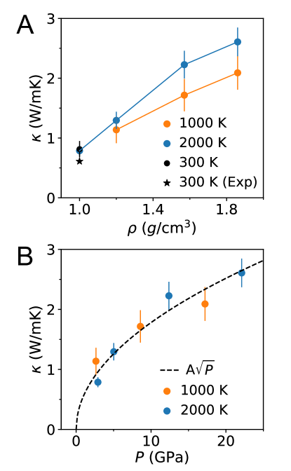
Figure 1: Thermal conductivity $\kappa$ of water at extreme conditions. A: dependence of $\kappa$ on density ($\rho$). We also show $\kappa$ at ambient conditions, i.e. the measured (300 K (Exp)) and computed (300 K) values. B: dependence of $\kappa$ on pressure ($P$). The dashed line is a simple fit $\kappa=A\sqrt{P}$ ($A\approx$ 0.56).

We now turn to analyzing the dependence of $\kappa$ on the temperature, density (Figure 1A) and pressure (Figure 1B). At the densities studied here, we find that the thermal conductivity increases slightly with $T$ from 1,000 to 2,000 K. Incidentally, the $\kappa$ for water at 1 g/cm³ and 2,000 K is almost the same as that computed at ambient conditions. Consistent with experimental data at lower temperature and pressure [12], and with high pressure studies of ice [13], our simulations show an increase of the thermal conductivity as the density and pressure are increased. In addition, our results are consistent with the simulation reported in Ref. [20], where the authors found that the thermal conductivity in the $T$-$\rho$ range investigated in our work is approximately independent on temperature. Remarkably, we find that a square root function $\kappa=A\sqrt{P}$ captures rather well the dependence of $\kappa$ on $P$, at both 1,000 and 2,000 K ($A$ is a parameter almost constant as a function of $T$, between 1,000 and 2,000 K). We quantify the relative error (RE) as:

$${\rm RE}=\frac{\lvert A\sqrt{P}-\kappa\rvert}{\kappa}\times 100\%$$ (6)

where the fitted $A$ ($\approx$ 0.56) was used, and $\kappa$ is the thermal conductivity from SAEMD simulations. We find the average RE over the 7 data points is 10.3 %; the maximum RE is 21.9 %.

In order to interpret the temperature, pressure and density dependence of $\kappa$, particularly the relation $\kappa=A\sqrt{P}$ found in our simulation, we employed a simple model, described below.

III.2 Model to interpret simulations

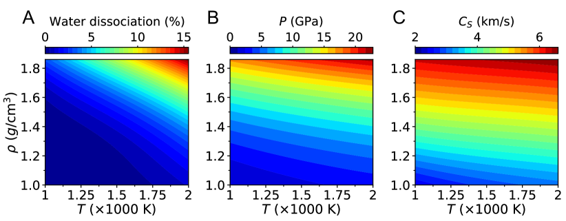
Figure 2: Interpolated physical properties of water at extreme conditions. A: the ratio of dissociated molecules; B: the pressure ($P$); C: the sound velocity ($C_{S}$).

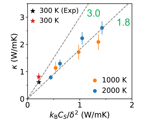
Figure 3: Validation of the model $\kappa=\widetilde{C_{V}}k_{\rm B}C_{S}/\delta^{2}$ (eq 7) used to interpret simulation data, where $\widetilde{C_{V}}$ is a fitting parameter. We show a dashed line for $\widetilde{C_{V}}\approx 1.8$, corresponding to the best fit of the values of $\kappa$ at extreme conditions. The measured (300 K (Exp)) and computed (300 K) values at ambient conditions are also shown using the measured sound velocity of water $\approx$ 1500 m/s, as well as a dashed line for $\widetilde{C_{V}}=3.0$.

Numerous models have been proposed in the literature to describe the thermal conductivity of liquids [46, 47, 48, 49]. Here we use a simple expression of $\kappa$ encompassing several of these models:

$$\kappa=\widetilde{C_{V}}k_{\rm B}C_{S}/\delta^{2}$$ (7)

where $\widetilde{C_{V}}$ is a model-dependent prefactor; $k_{\rm B}$ is the Boltzmann constant; $C_{S}$ is the sound velocity; $\delta=n^{-1/3}$ is the inter-molecular distance, where $n$ is the number density of the molecules in the fluid. In eq 7 one assumes that the amount of energy transferred during heat transport is proportional to $\widetilde{C_{V}}k_{\rm B}$ and that the speed of energy transfer is approximately equal to the sound velocity $C_{S}$; the energy is transferred step by step, between neighboring molecules separated by a distance $\delta$.

We extend the use of eq 7 to interpret the results of the thermal conductivity of water computed at extreme conditions. It should be noted that at HPT water may dissociate[15, 16, 50, 18, 19, 38]. Hence, we first verified whether the use of eq 7, derived for simple liquids with no dissociating units, is at least approximately justified. We computed the ratio of dissociated water molecules in our samples, as shown in Figure 2A. We found that even at the highest $T$ and $\rho$ studied here, less than $\sim$ 15 % of molecules were dissociated and therefore we expect that the dissociation of water molecules is not a major factor affecting thermal transport at the conditions considered in our work. Hence the use of the model of eq 7 appears to be reasonable to interpret our simulation results for HPT water.

Similar to previous studies, we use $\delta=(\rho/m_{0})^{-1/3}$, where $m_{0}$ is the mass of a water molecule. Using $\delta$ equal to the average O-O distance in water yields similar results. The value of $\widetilde{C_{V}}(T,\rho)$ and $C_{S}(T,\rho)$, the sound velocity of water at extreme conditions, are not available from the literature. We can obtain the $C_{S}(T,\rho)$ from our equation of state calculations for $E(T,\rho)$ and $P(T,\rho)$ (see Methods), shown in Figure 2B and 2C. However, we do not have well-defined methods to compute $\widetilde{C_{V}}(T,\rho)$, especially at HPT. In previous studies, $\widetilde{C_{V}}$ was approximated by the specific heat per molecule ($C_{V}$ or $C_{P}$) [47, 48, 49], e.g. $\widetilde{C_{V}}=C_{V}/k_{\rm B}$. This may be a good approximation for liquids, including water, at near ambient conditions, where the major contribution to the heat capacity comes from inter-molecular interactions. However, at extreme conditions and high temperature the contributions of intra-molecular vibrations cannot be ignored. Therefore, we would expect a serious error in our estimate of $\kappa$ if we used $\widetilde{C_{V}}$ as $C_{V}/k_{\rm B}$ in eq 7. Hence here we treat $\widetilde{C_{V}}$ as a parameter that we fit using the computed $\kappa$ at high $P$ and $T$ (the 7 data points in Table 1).

As shown in Figure 3, we obtain a reasonable linear fit of $\kappa$ versus $k_{\rm B}C_{S}/\delta^{2}$, from which we determine $\widetilde{C_{V}}$ $\approx$ 1.8. We quantify the RE as:

$${\rm RE}=\frac{\lvert\widetilde{C_{V}}k_{\rm B}C_{S}/\delta^{2}-\kappa\rvert}{\kappa}\times 100\%$$ (8)

where the fitted $\widetilde{C_{V}}$ ($\approx$ 1.8) was used, and $\kappa$ is the thermal conductivity from SAEMD simulations. We find that the average RE over the 7 data points is 9.5 %; the maximum RE is 17.7 %. The reasonable error found here indicates that water dissociation is unlikely to affect heat conduction in HPT water, in the $T$-$\rho$ range considered in our work. However, while dissociation remains limited, proton conduction via Grotthus like mechanisms might play a role in determining heat transport. This aspect has not been studied in detail here and also for this reason we chose to fit the $\widetilde{C_{V}}$ parameter to simulation data. To show qualitatively the difference between $\widetilde{C_{V}}$ at ambient and extreme conditions, in Figure 3 we plot two lines corresponding to a value of $\widetilde{C_{V}}$ equal to 3 and $\approx$ 1.8. When using $\widetilde{C_{V}}=3$ [51, 47], the measured value of $\kappa$ at ambient conditions can be correctly predicted. The smaller $\widetilde{C_{V}}$ ($\approx$ 1.8) found at HPT appears to be consistent with the presence of a disrupted hydrogen bonded network and a small fraction of dissociated water molecules at extreme conditions, leading to a decrease in the energy transfer between adjacent molecules, relative to ambient conditions.

We expect that treating $\widetilde{C_{V}}$ as a function of $T$ and $\rho$, instead of a fitting parameter (Figure 3), would increase the accuracy of the model (eq 7) in describing the thermal conductivity at HPT.

Using the model (eq 7) with the determined $\widetilde{C_{V}}$ ($\approx$ 1.8), we predicted the thermal conductivity in the whole $T$-$\rho$ range. Our results are shown in Figure 4. Based on the fitting error (Figure 3 and eq 8), the average RE of our predicted $\kappa$ should be approximately 10 % and the maximum RE $\sim$ 20 %. We note that due to finite-size effects, our prediction here may also be slightly under-estimated.

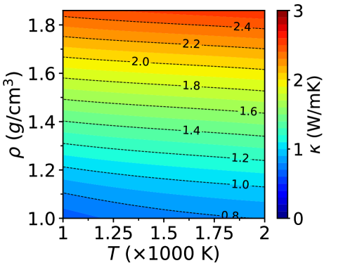
Figure 4: Predicted thermal conductivity $\kappa$ using the model (eq 7; see text).

Finally, by substituting $\delta=(\rho/m_{0})^{-1/3}$ into eq 7, we obtain the relation $\kappa\propto\rho^{2/3}C_{S}(T,\rho)$. As shown in Figure 2C, $C_{S}$ increases slightly with $T$ but significantly with $\rho$, which, according to the model (eq 7), leads to the same dependence found in our simulations for $\kappa$.

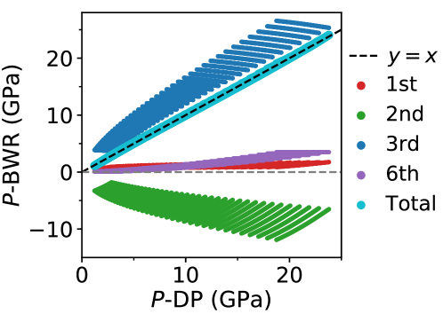
Figure 5: Pressure of water obtained with the Benedict–Webb–Rubin (BWR) equation ($P$-BWR) as a function of pressure computed in our simulations ($P$-DP). We show values for several $T$ and $\rho$ conditions. The contributions from virial terms (1st, 2nd, 3rd and 6th) to $P$-BWR are also shown. We plot a dashed line, $y=x$ as a guide to the eye, showing that $P$-BWR and $P$-DP values are close to each other. The $P$-BWR and $P$-DP are obtained on a dense grid, and the parameters in the BWR model are optimized (see text).

We note that $C_{S}$ is related to the derivative of $P$ (see Methods); hence an analytical formula for $P(T,\rho)$ is desirable to derive the relation between $C_{S}$ and $P$. To this end, we fit our interpolated function $P(T,\rho)$ using the Benedict–Webb–Rubin (BWR) equation [52, 53]:

$$P(T,\rho)=\frac{k_{\rm B}T}{m_{0}}\rho+(B_{0}T+B_{1})\rho^{2}+(C_{0}T+C_{1})\rho^{3}+D\rho^{6}$$ (9)

where $m_{0}$ is the mass of a water molecule; $B_{0}$, $B_{1}$, $C_{0}$, $C_{1}$ and $D$ are fitting parameters. We have ignored the exponential term and terms higher than $(1/T)^{0}$ for simplicity. Our fitting data, denoted as $P$-DP, are evenly spaced over a 100 $\times$ 40 mesh; at each grid point $T$-$\rho$, a value of $P$ is obtained from the interpolated function $P(T,\rho)$. We optimized the parameters entering the BWR equation and we show the computed pressure ($P$-BWR) in Figure 5, as well as the respective contributions. Interestingly, the BWR equation accurately describes the interpolated function $P(T,\rho)$, with a small root-mean-square-error of $\sim$ 0.07 GPa. We find that the 3rd-term is dominant; the contributions of 1st-, 2nd- and 6th-terms are smaller than that of the cubic one. We note an approximate cancellation between the sum of the positive 1st- and 6th-terms and the negative 2nd-term; the 3rd-term alone is of similar magnitude to the total pressure ($P$-BWR). Hence, for simplicity, we assume $P(T,\rho)\sim C(T)\rho^{3}$, where $C(T)$ refers to $C_{0}T+C_{1}$ in eq 9.

Knowing the dependence of the sound velocity on pressure and a form of the pressure as a function of temperature and density, we can now obtain an approximate dependence of $\kappa$ on the pressure:

$$\kappa\propto C_{S}/\delta^{2}\propto\rho^{2/3}\sqrt{\gamma\Bigl{(}\frac{\partial P}{\partial\rho}\Bigr{)}_{T}}\sim\rho^{1/6}\sqrt{\gamma\times 3C(T)\rho^{3}}\propto\rho^{1/6}\sqrt{\gamma}\sqrt{P}$$ (10)

where $\gamma$ is the adiabatic index (see Methods). In the $T$-$\rho$ range studied here, we find that $\sqrt{\gamma}$ and $\rho^{1/6}$ are in the range of $\sim$ (1.0, 1.1), i.e. nearly constant; as a result, we obtain that $\kappa\propto\sqrt{P}$. Although the square-root relation $\kappa\propto\sqrt{P}$ found here is not rigorously proven, it is a simple and useful functional relationship to approximately predict $\kappa$ when $P$ is measured in the range investigated in our work.

IV Conclusions

By carrying out SAEMD simulations with the DP potential, we computed the thermal conductivity of water at high temperatures, 1,000 $<T<$ 2,000 K and 1.0 $<\rho<$ 1.86 g/cm³, at conditions relevant to the Earth mantle. We found that the thermal conductivity depends weakly on the temperature and increases monotonically with the density and pressure, reaching values approximately 4 times larger than that at ambient conditions at the highest density point, indicating a more efficient heat energy transport under pressure than at ambient conditions. We showed that a simple model (eq 7) can satisfactorily describe the thermal conductivity of water at extreme conditions and using such a model we provided predictions of the thermal conductivity in a broad range of density and temperature. Our results indicate that the heat is transferred roughly at the speed of sound over nearest-neighbors inter-molecular distances, and that the heat conduction mechanism is not significantly affected by water dissociation, when the proportion of dissociated molecules remain smaller than 15 $\%$. Our simulations and the model used here to interpret them indicate that an increased sound velocity and density at extreme conditions are responsible for a larger thermal conductivity in HPT water than at ambient conditions. Numerically, we identified a square-root relationship between the thermal conductivity and the pressure of the system. Although this relationship is not rigorous, it can be useful to estimate the thermal conductivity at $T$-$\rho$ conditions similar to those studied here, since its direct measurement may be more difficult than that of the pressure. Our study provides both insights and useful data on transport properties and equation of states of water at high temperature and pressure, which may be useful in planetary and geo-sciences.

Notes

The authors declare no competing financial interest.

References

- Manning [2018] C. E. Manning, Fluids of the lower crust: deep is different, Annual Review of Earth and Planetary Sciences 46, 67 (2018).
- Nettelmann et al. [2013] N. Nettelmann, R. Helled, J. Fortney, and R. Redmer, New indication for a dichotomy in the interior structure of uranus and neptune from the application of modified shape and rotation data, Planetary and Space Science 77, 143 (2013).
- Zeng et al. [2019] L. Zeng, S. B. Jacobsen, D. D. Sasselov, M. I. Petaev, A. Vanderburg, M. Lopez-Morales, J. Perez-Mercader, T. R. Mattsson, G. Li, M. Z. Heising, et al., Growth model interpretation of planet size distribution, Proceedings of the National Academy of Sciences 116, 9723 (2019).
- Baraffe et al. [2010] I. Baraffe, G. Chabrier, and T. Barman, The physical properties of extra-solar planets, Reports on Progress in Physics 73, 016901 (2010).
- Guillot [2005] T. Guillot, The interiors of giant planets: Models and outstanding questions, Annu. Rev. Earth Planet. Sci. 33, 493 (2005).
- Fortney and Nettelmann [2010] J. J. Fortney and N. Nettelmann, The interior structure, composition, and evolution of giant planets, Space Science Reviews 152, 423 (2010).
- Schubert and Soderlund [2011] G. Schubert and K. M. Soderlund, Planetary magnetic fields: Observations and models, Physics of the Earth and Planetary Interiors 187, 92 (2011).
- Nettelmann et al. [2016] N. Nettelmann, K. Wang, J. J. Fortney, S. Hamel, S. Yellamilli, M. Bethkenhagen, and R. Redmer, Uranus evolution models with simple thermal boundary layers, Icarus 275, 107 (2016).
- Moll et al. [2017] R. Moll, P. Garaud, C. Mankovich, and J. Fortney, Double-diffusive erosion of the core of jupiter, The Astrophysical Journal 849, 24 (2017).
- Ross et al. [1984] R. G. Ross, P. Andersson, B. Sundqvist, and G. Backstrom, Thermal conductivity of solids and liquids under pressure, Reports on Progress in Physics 47, 1347 (1984).
- Huber et al. [2012] M. L. Huber, R. A. Perkins, D. G. Friend, J. V. Sengers, M. J. Assael, I. N. Metaxa, K. Miyagawa, R. Hellmann, and E. Vogel, New international formulation for the thermal conductivity of h2o, Journal of Physical and Chemical Reference Data 41, 033102 (2012).
- Abramson et al. [2001] E. H. Abramson, J. M. Brown, and L. J. Slutsky, The thermal diffusivity of water at high pressures and temperatures, The Journal of Chemical Physics 115, 10461 (2001).
- Chen et al. [2011] B. Chen, W.-P. Hsieh, D. G. Cahill, D. R. Trinkle, and J. Li, Thermal conductivity of compressed h 2 o to 22 gpa: A test of the leibfried-schlömann equation, Physical Review B 83, 132301 (2011).
- Zhao et al. [2020] G. Zhao, S. Shi, H. Xie, Q. Xu, M. Ding, X. Zhao, J. Yan, and D. Wang, Equation of state of water based on the scan meta-gga density functional, Physical Chemistry Chemical Physics 22, 4626 (2020).
- Rozsa et al. [2018] V. Rozsa, D. Pan, F. Giberti, and G. Galli, Ab initio spectroscopy and ionic conductivity of water under earth mantle conditions, Proceedings of the National Academy of Sciences 115, 6952 (2018).
- Zhang et al. [2020] C. Zhang, F. Giberti, E. Sevgen, J. J. de Pablo, F. Gygi, and G. Galli, Dissociation of salts in water under pressure, Nature communications 11, 3037 (2020).
- Pan et al. [2014] D. Pan, Q. Wan, and G. Galli, The refractive index and electronic gap of water and ice increase with increasing pressure, Nature communications 5, 3919 (2014).
- French et al. [2011] M. French, S. Hamel, and R. Redmer, Dynamical screening and ionic conductivity in water from ab initio simulations, Physical review letters 107, 185901 (2011).
- Goncharov et al. [2005] A. F. Goncharov, N. Goldman, L. E. Fried, J. C. Crowhurst, I.-F. W. Kuo, C. J. Mundy, and J. M. Zaug, Dynamic ionization of water under extreme conditions, Physical review letters 94, 125508 (2005).
- French [2019] M. French, Thermal conductivity of dissociating water—an ab initio study, New Journal of Physics 21, 023007 (2019).
- Marcolongo et al. [2016] A. Marcolongo, P. Umari, and S. Baroni, Microscopic theory and quantum simulation of atomic heat transport, Nature Physics 12, 80 (2016).
- Ercole et al. [2016] L. Ercole, A. Marcolongo, P. Umari, and S. Baroni, Gauge invariance of thermal transport coefficients, Journal of Low Temperature Physics 185, 79 (2016).
- Green [1952] M. S. Green, Markoff random processes and the statistical mechanics of time-dependent phenomena, The Journal of Chemical Physics 20, 1281 (1952).
- Green [1954] M. S. Green, Markoff random processes and the statistical mechanics of time-dependent phenomena. ii. irreversible processes in fluids, The Journal of chemical physics 22, 398 (1954).
- Kubo [1957] R. Kubo, Statistical-mechanical theory of irreversible processes. i. general theory and simple applications to magnetic and conduction problems, Journal of the Physical Society of Japan 12, 570 (1957).
- Kubo et al. [1957] R. Kubo, M. Yokota, and S. Nakajima, Statistical-mechanical theory of irreversible processes. ii. response to thermal disturbance, Journal of the Physical Society of Japan 12, 1203 (1957).
- Grasselli et al. [2020] F. Grasselli, L. Stixrude, and S. Baroni, Heat and charge transport in h2o at ice-giant conditions from ab initio molecular dynamics simulations, Nature Communications 11, 3605 (2020).
- Tisi et al. [2021] D. Tisi, L. Zhang, R. Bertossa, H. Wang, R. Car, and S. Baroni, Heat transport in liquid water from first-principles and deep neural network simulations, Physical Review B 104, 224202 (2021).
- Ercole et al. [2017] L. Ercole, A. Marcolongo, and S. Baroni, Accurate thermal conductivities from optimally short molecular dynamics simulations, Scientific reports 7, 15835 (2017).
- Bertossa et al. [2019] R. Bertossa, F. Grasselli, L. Ercole, and S. Baroni, Theory and numerical simulation of heat transport in multicomponent systems, Physical Review Letters 122, 255901 (2019).
- Puligheddu and Galli [2020] M. Puligheddu and G. Galli, Atomistic simulations of the thermal conductivity of liquids, Physical Review Materials 4, 053801 (2020).
- Wang et al. [2018] H. Wang, L. Zhang, J. Han, and E. Weinan, Deepmd-kit: A deep learning package for many-body potential energy representation and molecular dynamics, Computer Physics Communications 228, 178 (2018).
- Zhang et al. [2018a] L. Zhang, J. Han, H. Wang, R. Car, and E. Weinan, Deep potential molecular dynamics: a scalable model with the accuracy of quantum mechanics, Physical review letters 120, 143001 (2018a).
- Zhang et al. [2018b] L. Zhang, J. Han, H. Wang, W. Saidi, R. Car, et al., End-to-end symmetry preserving inter-atomic potential energy model for finite and extended systems, Advances in neural information processing systems 31 (2018b).
- Plimpton [1995] S. Plimpton, Fast parallel algorithms for short-range molecular dynamics, Journal of computational physics 117, 1 (1995).
- Thompson et al. [2022] A. P. Thompson, H. M. Aktulga, R. Berger, D. S. Bolintineanu, W. M. Brown, P. S. Crozier, P. J. in’t Veld, A. Kohlmeyer, S. G. Moore, T. D. Nguyen, et al., Lammps-a flexible simulation tool for particle-based materials modeling at the atomic, meso, and continuum scales, Computer Physics Communications 271, 108171 (2022).
- Sun et al. [2015] J. Sun, A. Ruzsinszky, and J. P. Perdew, Strongly constrained and appropriately normed semilocal density functional, Physical review letters 115, 036402 (2015).
- Zhang et al. [2021] L. Zhang, H. Wang, R. Car, and E. Weinan, Phase diagram of a deep potential water model, Physical review letters 126, 236001 (2021).
- Pedregosa et al. [2011] F. Pedregosa, G. Varoquaux, A. Gramfort, V. Michel, B. Thirion, O. Grisel, M. Blondel, P. Prettenhofer, R. Weiss, V. Dubourg, J. Vanderplas, A. Passos, D. Cournapeau, M. Brucher, M. Perrot, and E. Duchesnay, Scikit-learn: Machine learning in Python, Journal of Machine Learning Research 12, 2825 (2011).
- Cheng and Frenkel [2020] B. Cheng and D. Frenkel, Computing the heat conductivity of fluids from density fluctuations, Physical Review Letters 125, 130602 (2020).
- Alavi et al. [1995] A. Alavi, M. Parrinello, and D. Frenkel, Ab initio calculation of the sound velocity of dense hydrogen: implications for models of jupiter, Science 269, 1252 (1995).
- Powell et al. [1966] R. W. Powell, C. Y. Ho, and P. E. Liley, Thermal conductivity of selected materials, NIST reference data (1966), page 130.
- Ramires et al. [1995] M. L. V. Ramires, C. A. Nieto de Castro, Y. Nagasaka, A. Nagashima, M. J. Assael, and W. A. Wakeham, Standard reference data for the thermal conductivity of water, Journal of Physical and Chemical Reference Data 24, 1377 (1995), https://doi.org/10.1063/1.555963 .
- Piaggi et al. [2021] P. M. Piaggi, A. Z. Panagiotopoulos, P. G. Debenedetti, and R. Car, Phase equilibrium of water with hexagonal and cubic ice using the scan functional, Journal of Chemical Theory and Computation 17, 3065 (2021).
- Ceriotti et al. [2016] M. Ceriotti, W. Fang, P. G. Kusalik, R. H. McKenzie, A. Michaelides, M. A. Morales, and T. E. Markland, Nuclear quantum effects in water and aqueous systems: Experiment, theory, and current challenges, Chemical reviews 116, 7529 (2016).
- Bridgman [1923] P. W. Bridgman, The thermal conductivity of liquids under pressure, Proceedings of the American Academy of Arts and Sciences 59, 141 (1923).
- Khrapak [2021] S. A. Khrapak, Vibrational model of thermal conduction for fluids with soft interactions, Physical Review E 103, 013207 (2021).
- Zhao et al. [2021] A. Z. Zhao, M. C. Wingert, R. Chen, and J. E. Garay, Phonon gas model for thermal conductivity of dense, strongly interacting liquids, Journal of Applied Physics 129, 235101 (2021).
- Chen [2022] G. Chen, Perspectives on molecular-level understanding of thermophysics of liquids and future research directions, Journal of Heat Transfer 144 (2022).
- Ye et al. [2022] Z. Ye, C. Zhang, and G. Galli, Photoelectron spectra of water and simple aqueous solutions at extreme conditions, Faraday Discussions 236, 352 (2022).
- Xi et al. [2020] Q. Xi, J. Zhong, J. He, X. Xu, T. Nakayama, Y. Wang, J. Liu, J. Zhou, and B. Li, A ubiquitous thermal conductivity formula for liquids, polymer glass, and amorphous solids, Chinese Physics Letters 37, 104401 (2020).
- Benedict et al. [1940] M. Benedict, G. B. Webb, and L. C. Rubin, An empirical equation for thermodynamic properties of light hydrocarbons and their mixtures i. methane, ethane, propane and n-butane, The Journal of Chemical Physics 8, 334 (1940).
- Starling [1973] K. E. Starling, Fluid thermodynamic properties for light petroleum systems (Gulf Publishing Company, 1973).