The odd bunch: chrono-chemo-dynamics of sixteen unusual stars from Kepler

Abstract

In this study we combine asteroseismic, spectroscopic and kinematic information to perform a detailed analysis of a sample of 16 stars from the Kepler field. Our selection focuses on stars that appear to contradict Galactic chemical evolution models: young and $\alpha$-rich, old and metal-rich, as well as other targets with unclear classification in past surveys. Kinematics are derived from Gaia DR3 parallaxes and proper motions, and high-resolution spectra from HIRES/Keck are used to calculate chemical abundances for over 20 elements. This information is used to perform careful checks on asteroseismic masses and ages derived via grid-based modelling. Among the seven stars previously classified as young and $\alpha$-rich, only one seems to be an unambiguously older object masking its true age. We confirm the existence of two very old ($\geq$11 Gyr), super metal rich ($\geq$0.1 dex) giants. These two stars have regular thin disc chemistry and in-plane solar circle orbits which fit well in the picture of radial migration via the churning mechanism. The alternative explanation that these stars have younger ages would require mass-loss rates which strongly increases with increasing metallicity. Finally, we suggest further investigations to explore the suitability of Zn as a chemical clock in red giants.

1 Introduction

One of the well-established facts in nuclear astrophysics is that most chemical elements found in nature are synthesised inside stars (Burbidge et al., 1957; Nomoto et al., 2013; Tatischeff & Gabici, 2018; Kobayashi et al., 2020). That, along with the fact that stars largely conserve chemical information about their cosmic cradles in their atmospheres, means that we may use stellar abundances to probe the evolution of the Milky Way (hereafter, the Galaxy) and, in the bigger picture, of the Universe (Freeman & Bland-Hawthorn, 2002; Dotter et al., 2017).

In the past decade the advent of space based asteroseismology has allowed us to enrich the field of Galactic Archaeology by enabling measurements of masses and ages of a large number of red giants with unprecedented level of precision. Surveys such as those conducted by Yu et al. (2018) have provided asteroseismic information for more than 16,000 objects. As a consequence, now it is possible to examine Galactic evolution models in a more detailed manner (e.g., Stello et al., 2015; Zinn et al., 2022), in particular their information with respect to temporal evolution.

It has been observed that the Galactic disc has a spatial-temporal pattern regarding stellar abundances. Stars formed in the inner part of the disc tend to be more metal-rich than those formed in the outer disc at similar age (e.g., Schönrich & Binney, 2009; Bensby et al., 2011; Casagrande et al., 2011; Casagrande et al., 2016), and spatial dependence in the separation between high- and solar-$\alpha$ abundances is observed as well (e.g., Queiroz et al., 2020). Also, as a natural consequence of stellar nucleosynthesis, younger stars are expected to be more metal-rich than their older counterparts in the same Galactic environment. This is expected assuming a simplified ’closed-box’ evolution (Matteucci, 2021), but also in more refined scenarios (e.g., Spitoni et al., 2019). However, there is no clear age-metallicity relation in the solar neighbourhood (Edvardsson et al., 1993; Casagrande et al., 2011).

It has been proposed that the absence of an age-metallicity relation among stars in the solar neighbourhood is a consequence of stellar radial migration (Sellwood & Binney, 2002; Haywood, 2008; Roškar et al., 2008). That is also an explanation for the presence of super metal-rich stars in the solar circle (e.g., Trevisan et al., 2011, and references therein). On the other hand, the ages of some of these super metal-rich stars might be inaccurate (as commented by Pinsonneault et al., 2018, their ages for Red Clump stars must be taken with caution), a refinement of stellar evolution models may be required, leading to an improvement in the determination of fundamental stellar parameters. For instance, a better understanding of the Red Giant Branch (RGB) mass loss rate might improve our understanding of stars in the subsequent evolutionary stage, the Red Clump (RC).

Since the advent of Kepler (Koch et al., 2010) and CoRoT (Baglin et al., 2006), red giants identified as young and $\alpha$-rich have been extensively studied (Martig et al., 2015; Chiappini et al., 2015; Yong et al., 2016; Jofré et al., 2016; Matsuno et al., 2018; Silva Aguirre et al., 2018; Hekker & Johnson, 2019; Zhang et al., 2021; Jofré et al., 2023). These objects are interesting because the ratio between $\alpha$-elements and Fe is expected to decrease with the onset of Type-Ia Supernovae, which occurs relatively fast compared to the age of the Galactic disc (Matteucci & Recchi, 2001; Kilic et al., 2017). Many of the studies dissecting these anomalous $\alpha$-rich giants have suggested that their true ages have been masked by events of mass accretion. Hence, their current masses would be larger than their initial masses. Still, a detailed study may reveal more information about these interesting targets.

In that sense, our aim in this paper is to analyse a set of stars from the Galactic disc that have been previously identified as potential outliers with respect to chemical evolution models. We make use of the finest spectroscopic, asteroseismic, and astrometric information available to date for that set of targets. In Section 2 we summarise the sample under study, and in Section 3 we describe the methodology. Section 4 contains the results and discussion. Our final remarks are presented in Section 5.

2 Targets and observations

Table 1: Program stars, their adopted average seismic parameters and sources: (A) Yu et al. (2018), (B) Pinsonneault et al. (2018), (C) Casagrande et al. (2014), (D) This work. Parallaxes from Gaia DR2 and DR3 have zero-point calibrations from Zinn et al. (2019) and Lindegren et al. (2021), respectively.

KIC	RA	Dec	$\Delta\nu$	$\nu_{\mathrm{max}}$	Src	$\varpi_{\mathrm{DR2}}$	$\varpi_{\mathrm{DR3}}$
	(J2000)	(J2000)	$\mu$Hz	$\mu$Hz		mas	mas
KIC2845610	19 19 27.4059	+38 01 41.196	7.069 $\pm$ 0.052	91.65 $\pm$ 4.66	A	1.5878 $\pm$ 0.0292	1.6516 $\pm$ 0.0110
KIC3455760	19 37 45.7037	+38 35 35.637	4.860 $\pm$ 0.012	48.32 $\pm$ 0.50	A	1.0835 $\pm$ 0.0275	1.0080 $\pm$ 0.0131
KIC3833399	19 02 43.0468	+38 54 59.335	4.146 $\pm$ 0.024	37.12 $\pm$ 0.72	A	1.8780 $\pm$ 0.0236	1.7855 $\pm$ 0.0109
KIC5512910	18 55 30.9211	+40 42 44.672	4.337 $\pm$ 0.030	38.24 $\pm$ 0.71	A	0.2931 $\pm$ 0.0207	0.2571 $\pm$ 0.0138
KIC5707338	19 29 34.5475	+40 54 18.624	6.421 $\pm$ 0.037	81.89 $\pm$ 1.28	A	1.0415 $\pm$ 0.0317	1.0614 $\pm$ 0.0220
KIC6605673	19 26 41.3873	+42 03 41.578	68.010 $\pm$ 0.950	1263.00 $\pm$ 49.00	C	3.0358 $\pm$ 0.0254	2.9965 $\pm$ 0.0130
KIC6634419	19 54 48.4403	+42 04 29.868	7.238 $\pm$ 0.031	92.39 $\pm$ 2.11	A	$\cdots$	0.9982 $\pm$ 0.1695
KIC6936796	19 11 30.4158	+42 28 39.546	3.196 $\pm$ 0.044	22.36 $\pm$ 0.82	A	0.9443 $\pm$ 0.0206	0.8636 $\pm$ 0.0113
KIC6940126	19 16 27.6755	+42 28 23.477	21.610 $\pm$ 2.050	256.30 $\pm$ 1.30	D	0.9992 $\pm$ 0.0164	0.9475 $\pm$ 0.0132
KIC7595155	19 09 10.6703	+43 16 18.998	3.879 $\pm$ 0.044	28.95 $\pm$ 0.73	A	0.7125 $\pm$ 0.0225	0.6411 $\pm$ 0.0097
KIC8145677	18 50 43.8808	+44 03 14.383	4.513 $\pm$ 0.128	30.54 $\pm$ 0.34	A	0.7115 $\pm$ 0.0201	0.6105 $\pm$ 0.0103
KIC9002884	18 54 05.7764	+45 20 47.467	0.885 $\pm$ 0.029	4.70 $\pm$ 0.01	B	0.3859 $\pm$ 0.0203	0.2738 $\pm$ 0.0128
KIC9266192	18 57 05.5191	+45 43 28.972	6.317 $\pm$ 0.034	78.30 $\pm$ 5.94	A	1.6266 $\pm$ 0.0235	1.5940 $\pm$ 0.0119
KIC9761625	19 09 38.0164	+46 35 25.277	1.429 $\pm$ 0.023	9.23 $\pm$ 0.41	A	0.3996 $\pm$ 0.0228	0.3036 $\pm$ 0.0111
KIC10525475	19 10 21.3464	+47 43 19.394	4.335 $\pm$ 0.023	39.12 $\pm$ 0.91	A	0.9129 $\pm$ 0.0186	0.8508 $\pm$ 0.0100
KIC11823838	19 45 52.9235	+50 02 30.463	4.508 $\pm$ 0.025	42.70 $\pm$ 0.80	A	0.8634 $\pm$ 0.0269	0.7343 $\pm$ 0.0176

The high-resolution spectral data analysed in this paper were observed with the High Resolution Echelle Spectrometer (HIRES, Vogt et al., 1994) at the W. M. Keck Observatory, in the same campaign as the spectra studied by Alencastro Puls et al. (2022, hereafter Paper I). Data reduction was performed in the same method as in Paper I, using the Mauna Kea Echelle Extraction (makee) and iraf.

The stars present in this work are solar-like oscillators with available high-quality Kepler photometry (see Table 1 for their respective $\Delta\nu$ and $\nu_{\mathrm{max}}$ values) and [M/H] $>$ -0.5 dex – the more metal-poor objects from the observing run were analysed in Paper I. One of them – KIC 6605673 – is a main-sequence turnoff object, while the rest are red giants. The former was observed by Kepler in high-cadence mode, while the evolved stars have observations in low-cadence mode. All targets except KIC 6634419 have parallax measurements in both Gaia DR2 and (E)DR3 (Gaia Collaboration et al., 2018a, 2021, 2022). KIC 6634419 has a parallax measurement only in DR3, with precision of 17%, while DR2 precision in parallaxes are always below 7% in our sample. Fig. 1 shows how they compare to other giants in data from asteroseismic surveys.

The stars included in this study are divided into four groups: (i) APOKASC young $\alpha$-rich stars, red giants previously classified as young and $\alpha$-rich by Martig et al. (2015), and discussed in detail in Section 4.2, (ii) other group of red giants identified as old and metal-rich by Casagrande et al. (2014), analysed in Section 4.3, as well as (iii) four secondary clump objects with strong mode damping as evident by the very broad peaks in the frequency power spectra of their Kepler light curves, referred here as secondary RC stars. The last (iv) group (Group Four) contains three stars that do not fit in any of the previous three groups, and are discussed in Section 4.4 together with the secondary RC stars group. One of the Group Four stars, KIC 6940126, had been previously identified as old and metal-rich by Casagrande et al. (2014), but discussed separately in Section 4.1 due to its age uncertainty and location of its power excess near the Nyquist frequency. The other two were also studied by Casagrande et al., KIC 8145677 being identified as old and metal-poor, and KIC 6605673, classified as a metal-poor dwarf in their work.

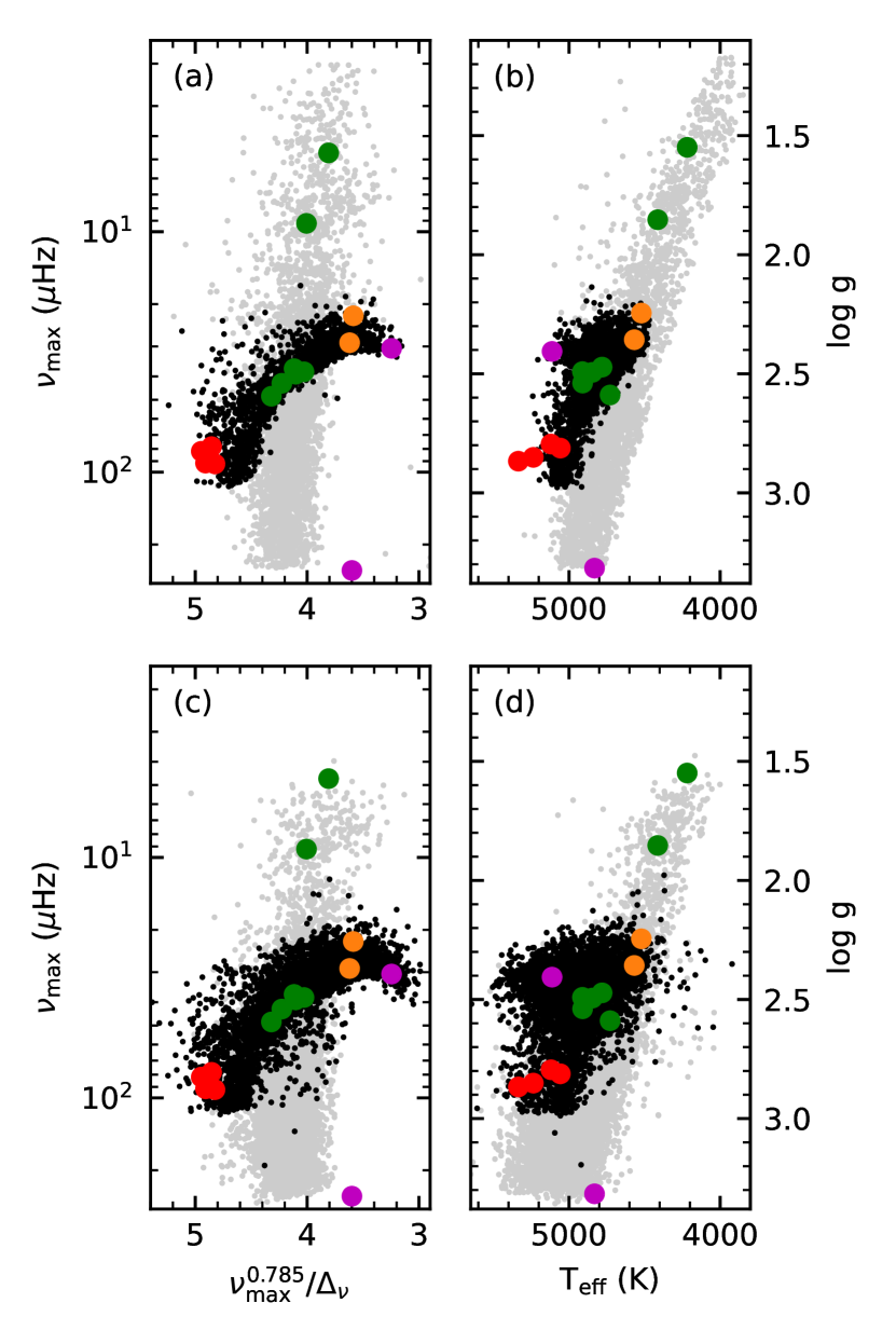
Figure 1: How our sample of red giants (circles) compares to the datasets from APOKASC-2 (Pinsonneault et al., 2018, panels (a) and (b)) and Yu et al. (2018, panels (c) and (d)). Black points are stars classified as core He-Burning in their works, while the grey points represent stars ascending the RGB. Circles’ colours represent the four groups enumerated in Section 2. Green: APOKASC young $\alpha$-rich stars. Orange: old and metal-rich. Red: secondary RC stars. Magenta: Group Four (KIC 6605673 not shown). The values for our sample are those adopted in this work (see Tables 1 and 2).

3 Analysis

This work combines chemical analysis from spectroscopic observations, grid-based asteroseismic modelling using Kepler data, and kinematics from Gaia. The methods are summarised in the following paragraphs. We refer to Paper I for a full methodological description, as both works share the same methodology.

Chemical abundances for 26 elements (Li, O, Na, Mg, Al, Si, Ca, Sc, Ti, V, Cr, Mn, Fe, Co, Ni, Cu, Zn, Sr, Y, Zr, Ba, La, Ce, Nd, Sm, Eu) were measured through the classical spectroscopic method, employing Gaussian fitting on weak isolated spectral lines for measuring their equivalent widths, whose values are shown in the supplementary material. For lines with blending and/or hyperfine splitting, spectral synthesis was employed – i.e., a synthetic spectrum was fitted using the 2017 version of moog (Sneden, 1973) to the observed one for each line under consideration. The line list was compiled from several sources (Cayrel et al., 2004; Alves-Brito et al., 2010; Meléndez et al., 2012; Barbuy et al., 2013; Ishigaki et al., 2013; Yong et al., 2014), and the log gf values from these sources were compared with those published in the NIST database. The log gf values from NIST were adopted when there was disagreement.

The atmospheric models required to translate equivalent widths in chemical abundances, as well as to build synthetic spectra, were interpolated from a solar-scaled plane-parallel 1D LTE ATLAS9/ODFNEW grid without overshooting (Castelli & Kurucz, 2003). The input atmospheric parameters required for interpolation (effective temperature T_eff, surface gravity log g, metallicity [M/H] and microturbulent velocity $v_{t}$) were defined as follows. First, a set of ’pure’ spectroscopic atmospheric parameters was calculated with moog using Fe i and Fe ii excitation/ionisation balance. [M/H] was estimated from [Fe/H] and [$\alpha$/Fe] using the formula from Salaris et al. (1993). The estimated log g and [M/H], as well as reddening from the 3D map from Green et al. (2019) and distances from Bailer-Jones et al. (2018), were used to feed the InfraRed Flux Method (IRFM, Blackwell & Shallis, 1977; Casagrande et al., 2010, 2021) employed to derive T_eff. Then, with [M/H] and the updated T_eff, log g was updated using asteroseismic information (see discussion in the next paragraph). New values of [M/H] and $v_{t}$ were calculated with moog, this time keeping the IRFM T_eff and the asteroseismic log g fixed. A new iteration was performed for each star until convergence was reached. Uncertainties for [M/H] and $v_{t}$ were calculated adapting the method from Epstein et al. (2010, see Paper I for details), while T_eff uncertainties were propagated from the IRFM inputs using MonteCarlo. The adopted atmospheric parameters are shown in Table 2. When compared to the initial spectroscopic guess, the IRFM effective temperatures tend to be slightly cooler (median difference is -71 $\pm$ 54 K), and the asteroseismic log g show a median difference of -0.12 $\pm$ 0.27 dex with respect to the spectroscopic ones. The median adopted values for metallicity and microturbulence differ by a small amount (-0.04 dex and -0.02 km s^-1, respectively), and present a small scatter as well (0.05 dex and 0.04 km s^-1). No trend between the differences in the methods with respect to the atmospheric parameters was detected, and the Pearson correlation coefficient between the results from the different methods is greater than 0.9 in all the four cases.

Table 2: The stellar parameters adopted to generate the atmospheric models for the spectroscopic analysis and their respective uncertainties.

Star	Teff	log g	[M/H]	$v_{t}$
	K	dex	dex	km s-1
KIC 2845610	5236 $\pm$  98	2.851 $\pm$ 0.006	0.05 $\pm$ 0.06	1.29 $\pm$ 0.05
KIC 3455760	4728 $\pm$109	2.589 $\pm$ 0.004	0.14 $\pm$ 0.08	1.19 $\pm$ 0.09
KIC 3833399	4781 $\pm$  68	2.472 $\pm$ 0.008	0.16 $\pm$ 0.06	1.45 $\pm$ 0.14
KIC 5512910	4911 $\pm$  95	2.491 $\pm$ 0.009	-0.19 $\pm$ 0.06	1.42 $\pm$ 0.05
KIC 5707338	5057 $\pm$  85	2.812 $\pm$ 0.003	0.23 $\pm$ 0.05	1.30 $\pm$ 0.10
KIC 6605673	5990 $\pm$  58	4.050 $\pm$ 0.008	-0.06 $\pm$ 0.03	1.05 $\pm$ 0.10
KIC 6634419	5335 $\pm$135	2.867 $\pm$ 0.004	0.19 $\pm$ 0.11	1.02 $\pm$ 0.18
KIC 6936796	4521 $\pm$  60	2.245 $\pm$ 0.012	0.19 $\pm$ 0.06	1.89 $\pm$ 0.15
KIC 6940126	4831 $\pm$  52	3.316 $\pm$ 0.003	0.26 $\pm$ 0.05	1.15 $\pm$ 0.14
KIC 7595155	4568 $\pm$  58	2.357 $\pm$ 0.009	0.28 $\pm$ 0.07	1.66 $\pm$ 0.21
KIC 8145677	5112 $\pm$  66	2.406 $\pm$ 0.005	-0.41 $\pm$ 0.04	1.56 $\pm$ 0.05
KIC 9002884	4218 $\pm$  50	1.549 $\pm$ 0.002	-0.14 $\pm$ 0.03	1.60 $\pm$ 0.12
KIC 9266192	5119 $\pm$  69	2.795 $\pm$ 0.006	0.14 $\pm$ 0.05	1.36 $\pm$ 0.11
KIC 9761625	4413 $\pm$  49	1.853 $\pm$ 0.014	-0.02 $\pm$ 0.03	1.45 $\pm$ 0.10
KIC 10525475	4845 $\pm$  59	2.494 $\pm$ 0.012	0.01 $\pm$ 0.04	1.27 $\pm$ 0.10
KIC 11823838	4910 $\pm$  72	2.539 $\pm$ 0.008	-0.18 $\pm$ 0.04	1.41 $\pm$ 0.05

Stellar ages, masses, radii, as well as log g, were derived with basta (BAyesian STellar Algorithm, Silva Aguirre et al., 2015, 2017; Aguirre Børsen-Koch et al., 2022). A set of observables were fitted for each star using the grid of BaSTI isochrones from (Hidalgo et al., 2018) and their mass loss prescription $\eta=$ 0.3. The chosen observables are equivalent to the s_n set from Paper I, i.e., the average asteroseismic parameters $\Delta\nu$ and $\nu_{\mathrm{max}}$ (with the correction from Serenelli et al., 2017), T_eff, [M/H], photometry in the 2MASS K_s band (Cutri et al., 2003), and a prior on the evolutionary phase which, for red giants, depends on the object position in the period spacing versus $\Delta\nu$ diagram (following Mosser et al., 2014) to differentiate those ascending the Red Giant Branch (RGB) from those in the Core-Helium Burning phase (CHeB). The uncertainties for the basta-derived parameters were taken from the 16th- and 84th- percentiles of their posterior distributions.

The sources of the asteroseismic parameters $\Delta\nu$ and $\nu_{\mathrm{max}}$ are listed in Table 1. For KIC 6940126 $\Delta\nu$ and $\nu_{\mathrm{max}}$ were estimated following the approach of Lund et al. (2016), adopting for $\nu_{\mathrm{max}}$ the fit of background model given by a sum of generalised Lorentzian functions with free exponents (Harvey, 1985; Karoff, 2012; Lund et al., 2017), including a Gaussian envelope centred on $\nu_{\mathrm{max}}$ to take into account the power excess from oscillations. The $\Delta\nu$ was measured from the peak of the power-of-power spectrum ($\rm PS\otimes PS$) centred on $\Delta\nu$/2, and the full width at half maximum of that peak corresponds to the $\Delta\nu$ uncertainty.

As in Paper I, orbital properties were determined for the sample using the Python-based galactic dynamics package, GalPy (Bovy, 2015). Orbits were initialised for each star using the astrometric properties from Gaia DR3, with the zero-point correction for parallaxes from Lindegren et al. (2021). Each orbit was integrated forward and backwards for 2 Gyr in the static Galactic potential of McMillan (2017). Galactic coordinates, local standard of rest and Solar position remained the same as in Paper I (Schönrich et al., 2010). In total, each orbit was integrated for 10-14 Gyr to determine the pericentric radii, apocentric radii, orbital energy, orbital eccentricity and maximum height from the plane (|Z|_max). The radial (J_r), azimuthal (equivalent to the z-component of the angular momentum, L_z) and z-actions (J_z) were determined using the Staekel fudge (Binney, 2012; Mackereth & Bovy, 2018). Finally, uncertainties were determined for each orbital property through determination of the covariance matrix associated with the Gaia DR3 astrometry. To sample the full error distribution of each input parameter, 1000 MonteCarlo realisations were made assuming a symmetric error distribution for the radial velocities.

4 Results and discussion

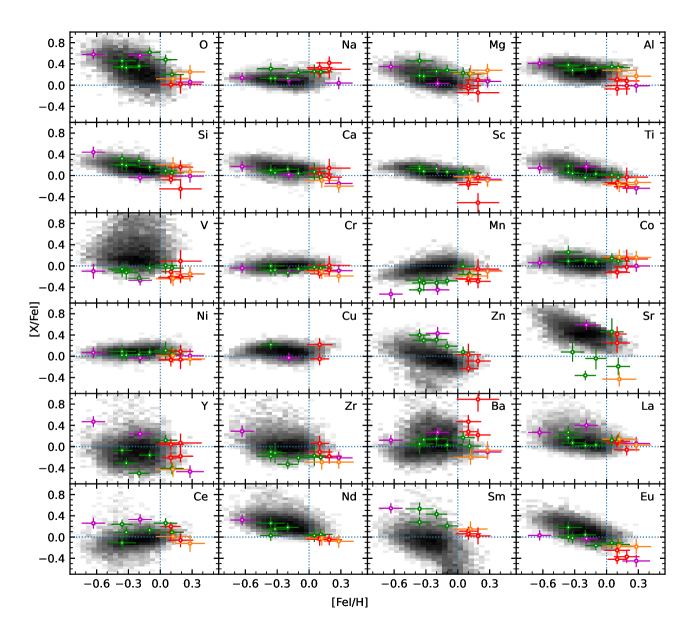
Figure 2: Abundance ratios [X/Fe i] as function of [Fe i/H] for all elements measured in this work other than Li. Point colours follow Fig. 1. The greyscale histograms represent the density of $\sim$ 9000 GALAH DR3 red giants (Buder et al., 2021) in the [X/Fe]-[Fe/H] space, shown here for guidance. Histogram intensity scales to log(N), where N is the number of stars from the selected GALAH sample. Blue dotted lines represent solar abundances. Histogram bin size is 0.05 $\times$ 0.05 dex.

Table 3: Abundance ratios A(Li) and [X/H]. Solar abundances are from Asplund et al. (2009).

KIC	A(Li)	[O/H]	[Na/H]	[Mg/H]	[Al/H]	[Si/H]	[Ca/H]	[Sc/H]	[Ti/H]
2845610	$\cdots$	0.11 $\pm$ 0.05	0.33 $\pm$ 0.09	0.04 $\pm$ 0.14	0.21 $\pm$ 0.14	0.02 $\pm$ 0.06	0.14 $\pm$ 0.08	-0.07 $\pm$ 0.04	-0.05 $\pm$ 0.12
3455760	$\cdots$	0.53 $\pm$ 0.05	0.31 $\pm$ 0.14	0.28 $\pm$ 0.10	0.40 $\pm$ 0.09	0.14 $\pm$ 0.12	0.12 $\pm$ 0.19	0.13 $\pm$ 0.04	0.06 $\pm$ 0.16
3833399	$\cdots$	0.31 $\pm$ 0.03	0.36 $\pm$ 0.09	0.32 $\pm$ 0.11	0.44 $\pm$ 0.06	0.16 $\pm$ 0.11	0.08 $\pm$ 0.08	0.16 $\pm$ 0.08	0.08 $\pm$ 0.12
5512910	$\cdots$	0.01 $\pm$ 0.05	-0.19 $\pm$ 0.07	-0.15 $\pm$ 0.04	-0.04 $\pm$ 0.07	-0.13 $\pm$ 0.10	-0.27 $\pm$ 0.12	-0.24 $\pm$ 0.04	-0.28 $\pm$ 0.14
5707338	$\cdots$	0.21 $\pm$ 0.02	0.61 $\pm$ 0.12	0.29 $\pm$ 0.11	0.27 $\pm$ 0.06	0.35 $\pm$ 0.13	0.16 $\pm$ 0.10	0.15 $\pm$ 0.07	-0.02 $\pm$ 0.11
6605673	2.61 $\pm$ 0.07	0.37 $\pm$ 0.07	-0.09 $\pm$ 0.12	-0.16 $\pm$ 0.05	$\cdots$	-0.23 $\pm$ 0.03	-0.17 $\pm$ 0.10	-0.07 $\pm$ 0.05	-0.02 $\pm$ 0.12
6634419	$\cdots$	0.21 $\pm$ 0.06	0.49 $\pm$ 0.12	0.05 $\pm$ 0.05	0.18 $\pm$ 0.12	-0.06 $\pm$ 0.03	0.33 $\pm$ 0.13	-0.32 $\pm$ 0.05	0.16 $\pm$ 0.15
6936796	$\cdots$	0.24 $\pm$ 0.02	$\cdots$	0.34 $\pm$ 0.01	0.40 $\pm$ 0.09	0.32 $\pm$ 0.13	0.03 $\pm$ 0.11	0.10 $\pm$ 0.13	-0.05 $\pm$ 0.11
6940126	$\cdots$	0.34 $\pm$ 0.01	0.32 $\pm$ 0.07	0.35 $\pm$ 0.05	0.27 $\pm$ 0.13	0.27 $\pm$ 0.11	0.13 $\pm$ 0.09	0.21 $\pm$ 0.06	0.04 $\pm$ 0.10
7595155	0.35 $\pm$ 0.11	0.53 $\pm$ 0.02	$\cdots$	0.56 $\pm$ 0.07	0.45 $\pm$ 0.14	0.35 $\pm$ 0.13	0.08 $\pm$ 0.08	0.19 $\pm$ 0.09	0.15 $\pm$ 0.12
8145677	$\cdots$	-0.05 $\pm$ 0.06	-0.49 $\pm$ 0.05	-0.28 $\pm$ 0.06	-0.22 $\pm$ 0.08	-0.19 $\pm$ 0.09	-0.46 $\pm$ 0.07	$\cdots$	-0.49 $\pm$ 0.10
9002884	$\cdots$	0.10 $\pm$ 0.03	-0.05 $\pm$ 0.08	0.10 $\pm$ 0.15	0.02 $\pm$ 0.12	-0.15 $\pm$ 0.12	-0.26 $\pm$ 0.09	-0.23 $\pm$ 0.03	-0.18 $\pm$ 0.14
9266192	$\cdots$	$\cdots$	0.43 $\pm$ 0.08	0.09 $\pm$ 0.12	0.03 $\pm$ 0.13	0.09 $\pm$ 0.06	0.13 $\pm$ 0.10	-0.03 $\pm$ 0.15	-0.03 $\pm$ 0.08
9761625	$\cdots$	0.16 $\pm$ 0.02	-0.07 $\pm$ 0.05	0.06 $\pm$ 0.04	0.11 $\pm$ 0.04	0.08 $\pm$ 0.11	-0.08 $\pm$ 0.09	-0.07 $\pm$ 0.08	-0.24 $\pm$ 0.08
10525475	$\cdots$	0.52 $\pm$ 0.01	0.14 $\pm$ 0.05	0.18 $\pm$ 0.11	0.23 $\pm$ 0.06	0.06 $\pm$ 0.07	-0.06 $\pm$ 0.10	-0.03 $\pm$ 0.08	-0.07 $\pm$ 0.12
11823838	$\cdots$	-0.01 $\pm$ 0.07	-0.23 $\pm$ 0.05	-0.18 $\pm$ 0.13	0.00 $\pm$ 0.09	-0.04 $\pm$ 0.08	-0.27 $\pm$ 0.09	-0.19 $\pm$ 0.04	-0.30 $\pm$ 0.09
KIC	[V/H]	[Cr/H]	[Mn/H]	[FeI/H]	[FeII/H]	[Co/H]	[Ni/H]	[Cu/H]	[Zn/H]
2845610	-0.01 $\pm$ 0.14	-0.05 $\pm$ 0.08	-0.15 $\pm$ 0.06	0.10 $\pm$ 0.09	0.01 $\pm$ 0.10	-0.01 $\pm$ 0.10	0.12 $\pm$ 0.10	0.05 $\pm$ 0.13	-0.13 $\pm$ 0.05
3455760	0.06 $\pm$ 0.18	0.03 $\pm$ 0.11	0.04 $\pm$ 0.15	0.05 $\pm$ 0.11	0.00 $\pm$ 0.18	0.19 $\pm$ 0.05	0.16 $\pm$ 0.19	$\cdots$	0.13 $\pm$ 0.09
3833399	0.07 $\pm$ 0.12	0.07 $\pm$ 0.08	-0.05 $\pm$ 0.09	0.11 $\pm$ 0.11	0.06 $\pm$ 0.10	0.20 $\pm$ 0.06	0.15 $\pm$ 0.16	$\cdots$	$\cdots$
5512910	-0.44 $\pm$ 0.16	-0.40 $\pm$ 0.10	-0.64 $\pm$ 0.18	-0.32 $\pm$ 0.11	-0.24 $\pm$ 0.12	$\cdots$	-0.30 $\pm$ 0.08	$\cdots$	-0.02 $\pm$ 0.08
5707338	-0.01 $\pm$ 0.12	0.11 $\pm$ 0.07	-0.10 $\pm$ 0.14	0.19 $\pm$ 0.12	0.20 $\pm$ 0.17	0.17 $\pm$ 0.07	0.28 $\pm$ 0.13	$\cdots$	0.10 $\pm$ 0.09
6605673	-0.46 $\pm$ 0.05	-0.30 $\pm$ 0.04	-0.64 $\pm$ 0.07	-0.19 $\pm$ 0.11	0.10 $\pm$ 0.08	$\cdots$	-0.22 $\pm$ 0.10	-0.22 $\pm$ 0.04	0.24 $\pm$ 0.13
6634419	0.28 $\pm$ 0.22	0.20 $\pm$ 0.14	0.13 $\pm$ 0.17	0.19 $\pm$ 0.20	0.33 $\pm$ 0.17	0.32 $\pm$ 0.13	0.13 $\pm$ 0.15	$\cdots$	$\cdots$
6936796	-0.12 $\pm$ 0.09	0.01 $\pm$ 0.09	-0.07 $\pm$ 0.11	0.12 $\pm$ 0.16	0.12 $\pm$ 0.15	0.29 $\pm$ 0.09	0.13 $\pm$ 0.09	$\cdots$	$\cdots$
6940126	0.13 $\pm$ 0.07	0.19 $\pm$ 0.08	0.19 $\pm$ 0.14	0.28 $\pm$ 0.13	0.24 $\pm$ 0.13	0.28 $\pm$ 0.06	0.29 $\pm$ 0.13	$\cdots$	$\cdots$
7595155	0.13 $\pm$ 0.14	0.09 $\pm$ 0.07	0.18 $\pm$ 0.15	0.28 $\pm$ 0.14	0.14 $\pm$ 0.12	0.44 $\pm$ 0.05	0.23 $\pm$ 0.10	$\cdots$	$\cdots$
8145677	-0.73 $\pm$ 0.16	-0.67 $\pm$ 0.05	-1.16 $\pm$ 0.09	-0.63 $\pm$ 0.11	-0.69 $\pm$ 0.12	-0.57 $\pm$ 0.10	-0.56 $\pm$ 0.09	$\cdots$	$\cdots$
9002884	-0.42 $\pm$ 0.12	-0.36 $\pm$ 0.09	-0.63 $\pm$ 0.16	-0.36 $\pm$ 0.13	-0.27 $\pm$ 0.19	-0.10 $\pm$ 0.01	-0.27 $\pm$ 0.12	$\cdots$	$\cdots$
9266192	-0.12 $\pm$ 0.10	0.02 $\pm$ 0.07	-0.14 $\pm$ 0.13	0.10 $\pm$ 0.12	0.22 $\pm$ 0.11	-0.02 $\pm$ 0.11	0.03 $\pm$ 0.12	0.32 $\pm$ 0.12	0.13 $\pm$ 0.24
9761625	-0.43 $\pm$ 0.06	-0.33 $\pm$ 0.06	-0.52 $\pm$ 0.12	-0.20 $\pm$ 0.10	-0.08 $\pm$ 0.17	-0.09 $\pm$ 0.02	-0.17 $\pm$ 0.17	$\cdots$	0.11 $\pm$ 0.08
10525475	-0.14 $\pm$ 0.11	-0.16 $\pm$ 0.06	-0.38 $\pm$ 0.08	-0.10 $\pm$ 0.10	-0.13 $\pm$ 0.13	-0.02 $\pm$ 0.04	-0.02 $\pm$ 0.16	$\cdots$	0.09 $\pm$ 0.08
11823838	-0.45 $\pm$ 0.13	-0.45 $\pm$ 0.06	-0.81 $\pm$ 0.07	-0.36 $\pm$ 0.10	-0.25 $\pm$ 0.14	-0.27 $\pm$ 0.08	-0.34 $\pm$ 0.11	-0.14 $\pm$ 0.06	0.04 $\pm$ 0.13
KIC	[Sr/H]	[Y/H]	[Zr/H]	[Ba/H]	[La/H]	[Ce/H]	[Nd/H]	[Sm/H]	[Eu/H]
2845610	0.52 $\pm$ 0.16	-0.11 $\pm$ 0.11	0.16 $\pm$ 0.17	0.38 $\pm$ 0.10	0.17 $\pm$ 0.05	0.30 $\pm$ 0.06	0.09 $\pm$ 0.08	0.21 $\pm$ 0.08	-0.32 $\pm$ 0.08
3455760	0.51 $\pm$ 0.29	0.17 $\pm$ 0.06	-0.12 $\pm$ 0.22	0.22 $\pm$ 0.10	0.17 $\pm$ 0.10	0.31 $\pm$ 0.07	0.08 $\pm$ 0.13	$\cdots$	-0.06 $\pm$ 0.03
3833399	-0.08 $\pm$ 0.19	-0.30 $\pm$ 0.11	-0.09 $\pm$ 0.13	0.12 $\pm$ 0.14	0.25 $\pm$ 0.08	0.20 $\pm$ 0.09	0.16 $\pm$ 0.09	$\cdots$	-0.03 $\pm$ 0.01
5512910	-0.24 $\pm$ 0.21	-0.63 $\pm$ 0.03	-0.44 $\pm$ 0.22	-0.19 $\pm$ 0.05	-0.25 $\pm$ 0.07	-0.23 $\pm$ 0.06	-0.17 $\pm$ 0.07	$\cdots$	-0.34 $\pm$ 0.02
5707338	$\cdots$	0.01 $\pm$ 0.11	0.01 $\pm$ 0.15	0.41 $\pm$ 0.12	0.13 $\pm$ 0.05	0.13 $\pm$ 0.14	0.14 $\pm$ 0.08	0.21 $\pm$ 0.18	-0.18 $\pm$ 0.00
6605673	0.40 $\pm$ 0.05	0.05 $\pm$ 0.11	$\cdots$	0.08 $\pm$ 0.04	0.21 $\pm$ 0.11	0.14 $\pm$ 0.03	$\cdots$	$\cdots$	-0.22 $\pm$ 0.04
6634419	$\cdots$	0.26 $\pm$ 0.12	$\cdots$	1.08 $\pm$ 0.25	$\cdots$	$\cdots$	$\cdots$	$\cdots$	$\cdots$
6936796	-0.31 $\pm$ 0.10	-0.31 $\pm$ 0.10	-0.17 $\pm$ 0.10	-0.08 $\pm$ 0.10	0.26 $\pm$ 0.05	0.13 $\pm$ 0.14	0.10 $\pm$ 0.09	0.27 $\pm$ 0.05	-0.05 $\pm$ 0.02
6940126	$\cdots$	-0.19 $\pm$ 0.10	0.07 $\pm$ 0.08	0.18 $\pm$ 0.14	0.34 $\pm$ 0.03	$\cdots$	$\cdots$	$\cdots$	-0.17 $\pm$ 0.04
7595155	$\cdots$	$\cdots$	-0.01 $\pm$ 0.08	0.21 $\pm$ 0.19	0.31 $\pm$ 0.06	0.16 $\pm$ 0.17	0.20 $\pm$ 0.08	$\cdots$	0.10 $\pm$ 0.01
8145677	$\cdots$	-0.16 $\pm$ 0.09	-0.34 $\pm$ 0.11	-0.51 $\pm$ 0.06	-0.36 $\pm$ 0.05	-0.37 $\pm$ 0.02	-0.31 $\pm$ 0.09	-0.09 $\pm$ 0.07	-0.60 $\pm$ 0.04
9002884	$\cdots$	$\cdots$	-0.54 $\pm$ 0.06	-0.31 $\pm$ 0.22	-0.19 $\pm$ 0.05	-0.47 $\pm$ 0.10	-0.10 $\pm$ 0.08	0.17 $\pm$ 0.10	-0.18 $\pm$ 0.04
9266192	0.35 $\pm$ 0.21	0.14 $\pm$ 0.09	0.00 $\pm$ 0.13	0.57 $\pm$ 0.13	0.20 $\pm$ 0.04	0.19 $\pm$ 0.14	0.06 $\pm$ 0.13	0.16 $\pm$ 0.02	-0.15 $\pm$ 0.06
9761625	-0.56 $\pm$ 0.07	-0.70 $\pm$ 0.06	-0.53 $\pm$ 0.08	-0.05 $\pm$ 0.16	-0.18 $\pm$ 0.03	$\cdots$	-0.02 $\pm$ 0.04	0.23 $\pm$ 0.04	-0.16 $\pm$ 0.02
10525475	-0.14 $\pm$ 0.24	-0.26 $\pm$ 0.06	-0.31 $\pm$ 0.10	-0.07 $\pm$ 0.12	-0.07 $\pm$ 0.07	0.03 $\pm$ 0.06	$\cdots$	0.11 $\pm$ 0.06	-0.26 $\pm$ 0.03
11823838	$\cdots$	-0.43 $\pm$ 0.02	-0.46 $\pm$ 0.13	-0.34 $\pm$ 0.05	-0.09 $\pm$ 0.14	-0.12 $\pm$ 0.03	-0.33 $\pm$ 0.11	-0.08 $\pm$ 0.09	-0.36 $\pm$ 0.01

Fig. 2 shows all abundances in terms of [X/Fe] derived in this work plotted as function of [Fe/H] – reference solar values are from Asplund et al. (2009). For comparison, abundance ratios of $\sim$9000 red giants from GALAH (Buder et al., 2021), selected in the same range of stellar parameters and parallaxes of the targets in our sample, are shown as greyscale clouds. For the majority of elements, the results from this study usually fall on the same range of abundance ratios for the respective metallicites in GALAH. For a handful of stars, there are possible outliers which lie on the edge of the GALAH distribution for the elements O, Na and Al. For the elements V, Mn, Zn and Sm, most of the sample appear offset from the GALAH distribution. Finally, for Sr and Y the sample exhibits a large scatter when compared to other elements.

The O abundances were obtained from the [O i] lines at 6300 Å and 6363 Å, measured by spectral synthesis. The 6300-line has a known blend with a Ni feature, and, for that reason, the spectral synthesis took into account the Ni abundances previously measured though EW. As seen in Fig. 2, the objects with anomalous O abundances do not have corresponding Ni anomalies, thus systematics arising from line blending could be discarded in their cases.

As for Na and Al, their abundances come from the usual lines employed in the literature for red giants: the Na i lines at 6154 Å and 6160 Å, as well as the Al i features at 6696 Å and 6698 Å. Although there is an average enhancement at solar metallicity – $\sim$ 0.2 dex in Na and $\sim$ 0.3 dex in Al, most data points fit inside the GALAH clouds in Fig. 2 for these species. Meanwhile, the distribution of Mn abundances – measured from the 6100 Å triplet with their hyperfine structure calculated using the same constants adopted by Barbuy et al. (2013) – follow the evolution of [Mn/Fe] versus [Fe/H] of the GALAH cloud, but in most cases shifted by at least $-$0.2 dex. The likely cause of that offset in Mn is the choice of log gf values, taken from the NIST database as mentioned in Section 3, which may be overestimated. This negative shift is apparent in the 6645 Å Eu ii abundances as well, albeit to a lesser extent. The results for [Mg/Fe] follow the typical distinction between ’high’ and ’normal’ Mg, which is not clear in the other individual $\alpha$ elements, Ca in particular. Two of the APOKASC young $\alpha$-rich giants – KIC 5512910, and KIC 11823838, and KIC 6605673, from Group Four, seem to fit clearly the lower (normal) envelope of the [Mg/Fe] GALAH distribution.

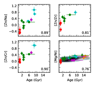
Figure 3: Selected abundance ratios which correlate with age. Numbers in the bottom right of each plot are the corresponding Pearson correlation coefficient. In all cases shown here the corresponding p-value is lower than 0.01. The density map in the bottom right plot combines APOKASC-2 and APOGEE-2 data (Pinsonneault et al., 2018; Jönsson et al., 2020), and their colour map scales to log(N), where N is the number of stars – darker representing higher density of objects. Colours as in Fig. 1, cyan circles are stars from Paper I. Ages for our data points were derived from pure asteroseismic solutions (see Section 4.1).

An element with intriguing results is Zn, despite the apparent $\sim$ 0.2 dex zero-point shift seen in Fig. 2 for [Zn/Fe]. In our dataset several abundance ratios that include Zn correlate with stellar ages – the strongest of them (Na, Cr, Zr) are shown in Fig. 3 with their respective correlation coefficients. These Zn-abundance ratios display steep gradients for chemical clocks, $\approx$ 0.1 dex Gyr^-1 from least-squares linear fits. Among the stars with Zn measurements, the metal-poor ones KIC 11563791 and KIC 4345370 (both analysed in Paper I) display strong enhancement in this species. Even if this pair is removed the correlation with age persists – Pearson correlation coefficient $\approx$ 0.75 in the three cases (when the two metal-poor stars from Paper I are ignored), p-value $<$ 0.01 in [Zn/Na], and $<$ 0.03 in [Zn/Cr] and [Zn/Zr]. Since our sample is relatively small and with strong selection effects, these intriguing correlations could be spurious.

In order to put the Zn results in perspective, the bottom right plot of Fig. 3 shows [Mg/Ni] as function of age. Despite also showing a strong correlation with age (Pearson coefficient is 0.76), the young and $\alpha$-rich stars (green markers), as well as the metal-poor targets studied in Paper I (cyan markers), show enhancement in [Mg/Ni] when compared to APOGEE-2/APOKASC-2 results (Jönsson et al., 2020; Pinsonneault et al., 2018). This may suggest that the stars in this study would not be suitable as chemical clocks, as, when we inspect our results against the APOGEE-2/APOKASC-2 results, our sample seems to be divided in high-[Mg/Ni] and normal-[Mg/Ni], the ’normal’ ones matching the space of highest density of the comparison sample ([Mg/Ni] $\lesssim$ +0.10). Nevertheless, a comprehensive high-precision study of Zn abundances in red giants with robust age determination (as done for solar twins by, e.g., Spina et al., 2016) could be extremely valuable.

We did check the magnitude of NLTE departures in four representative stars – KIC 2845610, KIC 6936796, KIC 8145677, KIC 9002884 – for the species available in the INSPECT database. We did find lines in common with our line list for Na, Mg, Ti, Fe i, and Fe ii (Bergemann, 2011; Lind et al., 2011; Lind et al., 2012; Bergemann et al., 2012; Osorio et al., 2015; Osorio & Barklem, 2016). The departures are mild except for Na, ranging between zero and $\sim$+0.05 dex. Thus, for most of the [X/Fe i] abundance ratios the NLTE departures of the individual species tend to cancel out. Fe ii NLTE corrections are estimated as -0.01 dex for all stars tested. For A(Na), the NLTE departures range from $\sim$-0.07 dex in the more metal-poor KIC 8145677 to $\sim$-0.12 dex in the more metal-rich stars tested. We did also check the MPIA tool in all stars for O, Si, Ca, Cr, Mn, and Co (Mashonkina et al., 2007; Bergemann & Cescutti, 2010; Bergemann et al., 2010, 2013; Bergemann et al., 2019, 2021; Voronov et al., 2022). Again, NLTE departures are mild ($\lesssim$ 0.05 dex), except for Co in KIC 8145677, whose NLTE departure increases A(Co) by 0.19 dex, or $\sim$2-$\sigma$. For Al, the expected NLTE correction in the 669-nm doublet measured in this work is assumed to be of the order of -0.05 dex in our stellar parameter range (Nordlander & Lind, 2017).

4.1 Grid-based modelling issues

As in Paper I, we performed grid-based modelling runs including and not including Gaia parallaxes. Given the differences in ages found for a few stars and their sensitivity to the parallax zero-point, we chose to adopt the ages calculated without taking parallaxes into account as their nominal ages. Here we will highlight two stars whose analysis presented a few issues.

A star with a large difference in ages calculated with and without Gaia DR2 parallaxes is Group Four target KIC 6940126. While the solution that does not take parallax into account gives an age of 8.4${}^{+5.2}_{-3.3}$ Gyr, the adoption of its Gaia DR2 parallax pushes the age towards the 20 Gyr grid limit, giving 18.3${}^{+1.2}_{-1.5}$ Gyr as the result. Neither of the two solutions is able to fit our estimated value of $\Delta\nu$ of 21.61 $\pm$ 2.05 $\mu$Hz inside an 1-$\sigma$ interval. It is important to note that the oscillation power excess of KIC 6940126 is near or above the Nyquist limit for Kepler’s low-cadence observations, and, thus, the determination of $\nu_{\mathrm{max}}$ might be problematic and unreliable, as the peak frequency might not be sampled appropriately. Despite the $\sim$ 10 Gyr difference in age between both solutions, the choice of which solution to use has no impact in the resulting abundances calculated for this object, because the difference in their estimated log g values is 0.003 dex.

The distance calculated for KIC 6940126 in the solution using parallax is 1021${}^{+8}_{-7}$ pc, in agreement with Bailer-Jones et al. (2018) (1018${}^{+18}_{-16}$ pc), and also with Bailer-Jones et al. (2021), which uses DR3 data (1012${}^{+13}_{-12}$ pc). On the other hand, the solution that ignores parallax provides a distance of 1137${}^{+62}_{-61}$ pc, resulting in a larger distance modulus, and, hence, an object with a larger intrinsic luminosity. The corresponding difference in the absolute K_s magnitude estimated in each of the solutions is 0.24 mag. Interestingly, if a basta run is done without the asteroseismic parameters in the input set, a solution taking the DR2 parallax value from Table 1 yields an age of 7.7${}^{+4.4}_{-2.6}$ Gyr, a distance of 1000${}^{+19}_{-18}$ pc, and $\Delta\nu$ = 22 $\pm$ 1 $\mu$Hz, in agreement with the $\Delta\nu$ shown in Table 1. However, that solution results in $\nu_{\mathrm{max}}$ = 342 $\pm$ 42 $\mu$Hz, and a corresponding log g of 3.44 $\pm$ 0.05 dex, 0.12 dex larger than the value adopted in Table 2. That 0.12 dex difference in log g might result in a non-negligible shift in the chemical abundances with respect to those abundances appearing in Table 3. The fitted [M/H] is not sensitive to these changes in basta input, at least for this star. In short, the stellar age derived using parallax instead of $\Delta\nu$ and $\nu_{\mathrm{max}}$ is more compatible with its super-solar metallicity, and higher-cadence observations would be necessary for an asteroseismic confirmation. Also, when compared to asteroseismic data in the literature (see Fig. 4), the super-Nyquist $\nu_{\mathrm{max}}$ resulting from the non-seismic constrained basta run for KIC 6940126 seems (by inspection) to have a better agreement with the overall $\Delta\nu$-$\nu_{\mathrm{max}}$ relation for red giants.

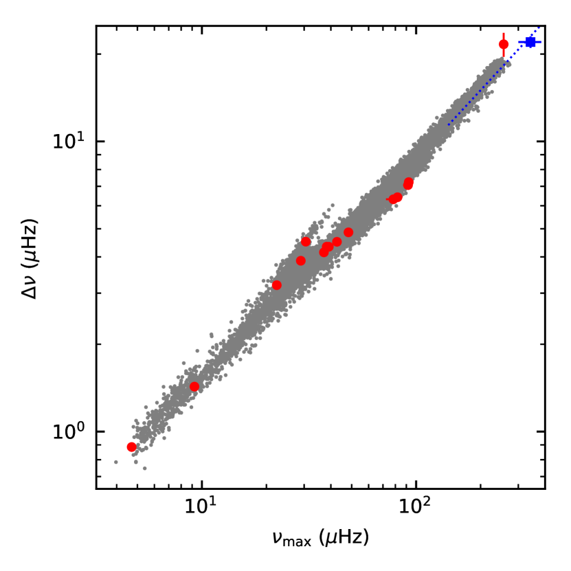
Figure 4: $\Delta\nu$ as function of $\nu_{\mathrm{max}}$. Red circles: values adopted for stars in this work (main-sequence star KIC 6605673 not shown). Grey points: data from Yu et al. (2018). The blue dotted line represents the linear fit for $\nu_{\mathrm{max}}>$ 300 $\mu$Hz from Huber et al. (2011, SYD pipeline). The blue square shows the basta solution for KIC 6940126 when no asteroseismic parameters are used in the input data (see text for discussion).

The grid-based modelling of KIC 9002884, one of the $\alpha$-rich stars from Martig et al. (2015), has given problematic results – not only the age uncertainties are large with the 16th- and 84th-percentiles corresponding to 6.8 and 16.9 Gyr, but the age distribution is bimodal with a secondary peak at $\approx$8 Gyr. The ages adopted in this work are the medians of the basta posteriors, for KIC 9002884 the median is 13.1 Gyr. If we use the Gaia DR2 parallax from Table 1, the median is similar, the uncertainties decrease, the secondary peak vanishes, and the estimated age becomes 13.4${}^{+2.1}_{-1.5}$ Gyr. However, when its Gaia DR3 parallax is included in the input its age drops to 2.6${}^{+0.5}_{-0.5}$ Gyr, not only a huge quantitative swing, but resulting in an entirely different interpretation about its nature from the qualitative point of view. We have undertaken three tests in basta excluding $\Delta\nu$ and $\nu_{\mathrm{max}}$ information and using Gaia DR2 or DR3 parallaxes. Both yielded large uncertainties as expected, while the median ages for the DR2 and DR3 experiments are similar to those estimated when asteroseismic information is included alongside with the respective parallax values.

From the test described above it seems that grid-based modelling is sensitive to the parallax in this object. Looking at the fitted asteroseismic parameters may give us a clue: two basta runs, one excluding parallax information, and another adopting DR2 parallax, give similar ages around 13 Gyr for KIC 9002884 and result in a $\Delta\nu$ value of 0.90 $\mu$Hz near the observed value of 0.885 $\pm$ 0.029 $\mu$Hz. Meanwhile, the basta run that adopts the DR3 parallax estimates 0.82 $\mu$Hz for $\Delta\nu$. All runs result in the same value of $\nu_{\mathrm{max}}$ – 4.70 $\mu$Hz. For constant $\nu_{\mathrm{max}}$ and T_eff, stellar mass scales with the inverse of $\Delta\nu$, which is observed in the younger age (i.e., larger mass) estimated with the DR3 parallax.

It is important to note that the large swing in age seen for KIC 9002884, from $\approx$13 Gyr to 2.6 Gyr, is likely due to the large difference between Gaia DR2 and DR3 parallaxes. The DR2 value of 0.3859 $\pm$ 0.0203 mas listed in Table 1 is 0.1121 mas larger than the DR3 parallax $\varpi=$ 0.2738 $\pm$ 0.0128 mas, corrected according to the prescription from Lindegren et al. (2021). That difference is larger than 5-$\sigma$ if we consider the DR2 uncertainty, or larger than 8-$\sigma$ if the DR3 uncertainty is to be considered. Besides the possible systematic underestimation of the DR3 uncertainties suggested in Paper I, inaccuracies in zero-point corrections or in the astrometric solutions themselves might be sources of error.

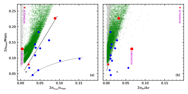
Figure 5: 2-$\sigma$ (84th- minus 16th-percentile) fractional uncertainties in mass against 2-$\sigma$ fractional uncertainties in $\nu_{\mathrm{max}}$ (a) and 2-$\sigma$ fractional uncertainties in $\Delta\nu$ (b). Marker sizes scale linearly with radii. Colours indicate evolutionary stage. Black: Main-Sequence. Red: Red Giant Branch. Blue: Core Helium Burning phase. Linear (dashed line) and logarithmic fits (dotted line) to our data are placed to guide the eye. Green dots are data from Yu et al. (2018), while grey dots represent data from APOKASC-2 (Pinsonneault et al., 2018). Anomalous stars in this study are labelled (see text for discussion).

Given the importance of ages in reconstructing Galactic evolution, a fundamental question we raise is which solution should we trust? From our tests, the large swing in Gaia parallaxes from DR2 to DR3 is biasing the estimated ages. Hence, the (very old) age calculated without adopting parallaxes seems to be more accurate. However, the previously mentioned double peak in the age distribution and its large uncertainties (when no parallax is considered) still pose a problem for the analysis of this star, suggesting a lack of accuracy in at least one of the observables. As an additional check, we did compare the angular diameter derived with radii and distances from basta solutions with that calculated with the IRFM: 0.094 $\pm$ 0.004 mas (the uncertainty is based on a conservative estimate of 4%, see Table 9 for the other stars). The fitted surface gravity values differ by less than 0.005 dex, and the more massive DR3-based solution gives a larger stellar radius for KIC 9002884. All three asteroseismic angular diameters calculated from the output of each run are inside the IRFM uncertainty, even if we consider 2% instead of 4% for the uncertainty estimation. Comparing the Gaia-based distances from Bailer-Jones et al. (2018) and Bailer-Jones et al. (2021), which use data from DR2 and DR3, respectively, the distances derived by Bailer-Jones et al. (2021) are $\approx$200 pc larger than the value of 2816${}^{+173}_{-155}$ pc from Bailer-Jones et al. (2018). We have also found a larger distance in our DR3-based solution, 3349${}^{+88}_{-135}$ pc, while the distances derived with the DR2 parallax and without parallax are basically the same: 2628${}^{+32}_{-42}$ pc and 2636${}^{+48}_{-47}$ pc, respectively. Given the discrepancy between Gaia DR2 and DR3 for this object, adopting ages calculated without parallax input for the whole sample seems to be the safest decision in this work, as it was done in Paper I, despite resulting in larger error bars.

In Fig. 5 the relative uncertainties of mass as function of the relative uncertainties in the average asteroseismic observables are shown. The two targets discussed in the previous paragraphs are highlighted in the plots, and it can be seen that both deviate from the overall trend. In the case of relative $\nu_{\mathrm{max}}$ uncertainty, we can also see that the group of secondary RC stars, discussed in Section 4.4, follow a particular trend. Fig 5 strongly suggests that our method is able to yield masses with better precision when compared to the large-scale surveys shown in comparison, as it tends to result in more precise masses for the same level of precision in $\Delta\nu$ and $\nu_{\mathrm{max}}$.

4.2 APOKASC young alpha-rich stars

Martig et al. (2015) investigated age-abundance relations using the first data release of APOKASC (Pinsonneault et al., 2014). They identified 14 $\alpha$-rich stars younger than 6 Gyr (out of a sample of 241), seven of which we observed as part of this project, and which we discuss in more detail below. Their seismic-derived parameters as well as their $\alpha$ abundances calculated in this study are shown in Table 4. Four of these stars are included in Matsuno et al. (2018), whose [Fe/H] values are systematically lower by 0.2-0.3 dex than in this work.

Table 4: Fitted parameters and $\alpha$ abundances for young stars characterized as $\alpha$-rich by Martig et al. (2015). Here, the objects in the core He-burning phase (marked with an asterisk) have radii between 11 and 12 R_⊙. The remaining stars are ascending the RGB. The objects with high probability of belonging to binary systems (Jofré et al., 2016) are marked with a dagger symbol.

KIC	Age	Mass	Radius	$[\alpha$/FeI$]$
	(Gyr)	(M⊙)	(R⊙)	dex
†3455760	2.8${}^{+0.5}_{-0.3}$	1.51${}^{+0.05}_{-0.07}$	10.3${}^{+0.1}_{-0.2}$	0.10 $\pm$ 0.09
3833399	3.0${}^{+0.6}_{-0.4}$	1.43${}^{+0.10}_{-0.09}$	11.5${}^{+0.3}_{-0.3}$	0.05 $\pm$ 0.06
†*5512910	2.8${}^{+0.6}_{-0.5}$	1.39${}^{+0.09}_{-0.11}$	11.1${}^{+0.3}_{-0.3}$	0.11 $\pm$ 0.08
†9002884	13.1${}^{+3.8}_{-6.3}$	0.92${}^{+0.16}_{-0.06}$	26.9${}^{+1.0}_{-0.7}$	0.24 $\pm$ 0.11
9761625	5.9${}^{+3.5}_{-1.8}$	1.19${}^{+0.13}_{-0.14}$	21.4${}^{+0.9}_{-1.0}$	0.16 $\pm$ 0.07
†*10525475	2.9${}^{+1.1}_{-0.5}$	1.42${}^{+0.11}_{-0.15}$	11.1${}^{+0.3}_{-0.5}$	0.13 $\pm$ 0.07
†*11823838	1.8${}^{+0.3}_{-0.2}$	1.66${}^{+0.07}_{-0.11}$	11.4${}^{+0.2}_{-0.3}$	0.16 $\pm$ 0.08

Of the seven stars in common with Martig et al. (2015), five are indeed young (or seem to be young). One of them, KIC 3833399, has solar [$\alpha$/Fe], and KIC 5512910 sits on the boundary between $\alpha$-rich and $\alpha$-normal defined by the white line in Fig. 6. Also, while most of the stars discussed in this Section seem visually $\alpha$-rich in Fig. 6, it is important to point out that only two have their [$\alpha$/Fe] differing from solar by more than 2-$\sigma$. Still, while adding this caveat that their status as $\alpha$-rich is disputed, we adopt the nomenclature for consistency with previous works in the literature. Finally, there are two stars which instead do not seem necessarily too young and we discuss them to follow.

In this work, KIC 9761625 sits on the limit for ’young’ stars as defined by Martig et al. (2015) for both age and mass (6 Gyr and 1.2 M_⊙, respectively). In order to check whether the differences in the adopted input observables were relevant, we replaced our values of $\nu_{\mathrm{max}}$, $\Delta\nu$, T_eff, and [M/H] with those published by Martig et al. for this object, as well as their adopted solar reference values. The grid-based modelling returned roughly the same age and mass as those shown in Table 4 ($\sim$6 Gyr and $\sim$1.2 M_⊙). If no model-based correction is applied to $\Delta\nu$ – using the paramter dnuscal instead of dnuSer in basta – the resulting mass is increased to 1.29 $\pm$ 0.12 M_⊙. This mass value is within the error bar from Martig et al. and, interestingly, it is the same mass published by APOKASC-2, where a scaling relation correction was applied. The average seismic parameters adopted here for KIC 9761625 have been taken from Yu et al. (2018), whose published (corrected) mass is 1.35 $\pm$ 0.21 M_⊙. However, the T_eff adopted by Yu et al. is 200 K hotter than that shown in Table 2, and a mass larger by $\sim$ 0.1 M_⊙ in the scaling relation could be attributed to a difference in temperature of that magnitude.

Despite being previously classified as ’young $\alpha$-rich’ by Martig et al. (2015) and ’$\alpha$-normal’ by Hekker & Johnson (2019, see discussion later in this subsection), KIC 9002884 has an age estimation of 13.1${}^{+3.8}_{-6.3}$ Gyr in this work, with $\alpha$-enhancement, i.e., its chemistry suggests that this object is indeed old ([$\alpha$/Fe] = +0.24 $\pm$ 0.11, see Table 4). This star has a problematic age determination, already discussed in Section 4.1. From the chemical perspective, KIC 9002884 displays enhancement in species such as Mg and Eu, seen in Fig. 2 as the most enhanced green circle for both species. This could be an indication that this object would be an old member of the Thick Disc or the Bulge that currently inhabits the solar circle. However, asteroseismic data of higher quality than Kepler’s is needed to constrain its fundamental parameters and to refine the analysis.

4.2.1 Differences in Fe i and Fe ii yield distinct interpretations

In their near-infrared analysis, Hekker & Johnson (2019) classified the stars in their sample as either ’young $\alpha$-rich’, ’old $\alpha$-rich’ or ’$\alpha$-normal’. Here, [$\alpha$/Fe] is defined as the average of [X_i/Fe], X_i = (Mg, Si, Ca, Ti), the same definition employed by Hekker & Johnson. In their work, KIC 5512910, KIC 10525475 and KIC 11823838 were classified as ’young $\alpha$-rich’. The other four stars in Table 4 were classified by Hekker & Johnson as ’$\alpha$-normal’, i.e., young stars that do not display $\alpha$-enhancement.

Among those $\alpha$-normal in the Hekker & Johnson (2019) sample is KIC 9002884, for which we obtain [$\alpha$/Fe] $=$ 0.24 in contrast with [$\alpha$/Fe] $=$ 0.07 measured in their work. It is interesting to point out, however, that in the case of KIC 9002884 both studies give similar [$\alpha$/H] values, $-$0.08 dex in case of Hekker & Johnson, $-$0.12 dex in this work, with the [Fe/H] calculated here being 0.21 dex lower, which pushes [$\alpha$/Fe] to 0.24 dex.

It must be noted that Hekker & Johnson (2019) Fe measurements are from Fe i, while in this study we did measure both Fe i and Fe ii lines. Because of our adoption of asteroseismic log g, which is assumed to be both more accurate and more precise than the spectroscopic one, we did not enforce ionisation balance. That means that Fe i and Fe ii abundances are not required to provide identical values, but, as shown in Fig. 6, our results allow for different qualitative interpretations for Fe (and $\alpha$) abundances depending on the ionisation state chosen for this chemical element. If we choose Fe i, we find that all stars are consistent with being $\alpha$-rich – above the white dash-dotted line in Fig. 6. Two of them, KIC 3833399 and KIC 5512910, have their data points lying near the boundary between $\alpha$-normal and $\alpha$-rich, which was based on the APOGEE-2 distribution also shown in Fig. 6.

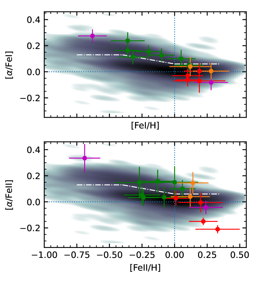
Figure 6: [$\alpha$/Fe] as function of [Fe/H] normalised for both Fe i (top) and Fe ii (bottom). Point colours follow Fig. 1, and density maps are described in Fig. 3. The white dash-dotted line represents the border between $\alpha$-rich and $\alpha$-normal adopted in this study. The abundance densities shown in greyscale are [Mg,Si,Ca,Ti/Fe] from APOGEE-2 (Jönsson et al., 2020).

When Fe ii is taken as representative for Fe, however, the interpretation changes. Three stars – KIC 5512910, KIC 9761625 and KIC 11823838 – are now on the $\alpha$-normal region, two of them in disagreement with the results from Hekker & Johnson. In some cases there is substantial disagreement between abundances from both Fe species, although the uncertainties overlap (see Table 3).

All these stars except KIC 3833399 were included in the study from Jofré et al. (2016) that estimated the probabilities p_b of these objects being in binary systems. The targets shown in Table 4 and studied by Jofré et al. have p_b = 1, except KIC 9761625 (p_b = 0.06). This star is one of the three objects in this subset that look ’$\alpha$-normal’, i.e., below the white dash-dotted line in Fig. 6 if $\alpha$ abundances are normalised by Fe ii instead of Fe i. The combination of $\alpha$-enhancement and binarity would give a strong hint on these stars being evolved blue stragglers, as the rate of binary systems is much higher in blue stragglers than in ’normal’ objects, and a past mass accretion event would mask an old, $\alpha$-rich red giant as a young $\alpha$-rich star (Yong et al. (2016) and references therein, but see Jofré et al. (2023)).

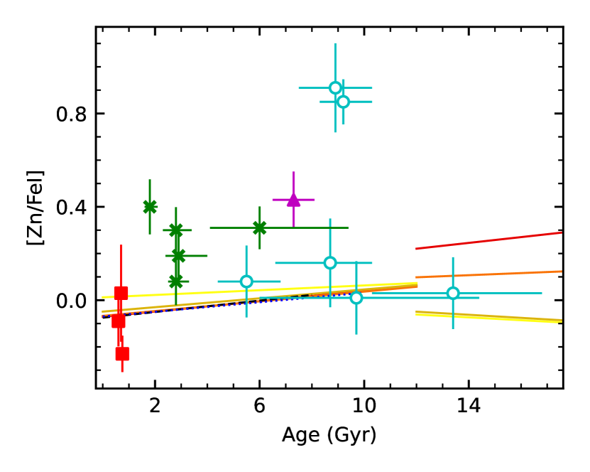
Figure 7: [Zn/Fe] as function of stellar age. Marker colours are the same as in Fig. 1. The magenta triangle is KIC 6605673, a dwarf. Cyan open circles are metal-poor objects from Paper I. Solid lines show [Zn/Fe] vs. age linear fits for different metallicity bins calculated by Lin et al. (2020) for main-sequence turnoff stars and subgiants using GALAH abundances (Buder et al., 2018). Line colours represent the [Fe/H] bins adopted by Lin et al., [-0.5, -0.1]: red, [-0.1, 0.0]: orange, [0.0, 0.1]: gold, and [0.1, 0.5]: yellow. The black dashed line represents the linear fit calculated by Spina et al. (2016) using solar twins.

4.2.2 Going beyond $\alpha$ abundances

While the information given by the $\alpha$ abundances is inconclusive on the status of this subset, Zn could be useful to shed some light on the discussion. [Zn/Fe] is plotted as function of stellar age in Fig. 7 for all stars with Zn measurements in this study and in Paper I. The plot also shows linear fits made by Spina et al. (2016) and Lin et al. (2020) in their age-abundance studies for solar-type and subgiant stars, respectively. The stars from Table 4 (green crosses in Fig. 7) display a systematic excess of Zn that is also detected for Mg in the age-[Mg/Ni] relation from Fig. 3. This excess seems consistent with the interpretation that their chemistry is indicative of older ages than derived from their masses. In both cases, our young metal-rich RC stars (to be discussed in Section 4.4, and here assumed to be chemically normal stars), can be used to anchor our metallicity scale against the APOGEE-2 cloud from Fig. 3 and the linear fits from Fig. 7. Given that both Mg and Zn are tracers from core-collpase supernovae (Nomoto et al., 2013; Kobayashi et al., 2020), from their chemistry alone it is unlikely that these stars are young thin disc objects. Also, binarity has been detected by radial velocity monitoring for most of these objects, as mentioned in the previous paragraph, hinting on the possibility of past mass accretion events for each of these red giants, making them look younger than they would actually be. The fact that their ages are possibly masked by past mass accretion events has been already pointed by Jofré et al. (2016).

However, for KIC 5512910 and KIC 11823838 the interpretation becomes complicated if we consider the Mg abundance normalised by Fe i. Their [Mg/Fe] abundance ratios fall in the intermediate region between normal- and enhanced-Mg in Fig. 2 – the same happens for Si, Ca, and Ti. Considering the error bars these two objects could be either normal or enhanced for these species. Also, when the orbits are taken into account (see Table 6) the scenario becomes even more unclear. If we assume that the stars being discussed here in Section 4.2, with the exception of KIC 9002884, are old $\alpha$-rich objects that did experience mass accretion events in the past, one would expect thick disc-like orbits. Nevertheless, our orbital modelling from Gaia data shows that three of them – KIC 3455760, KIC 3833399 and KIC 11823838 – have |Z_max| < 0.5 kpc, and action J${}_{\mathrm{z}}<$ 5 kpc km s^-1, staying close to the Galactic plane. Of these three, KIC 3833399 in particular does not seem to fit in the false-young $\alpha$-rich categorisation with the data we currently have available, due to its low $\alpha$ abundance. It is one of the two stars near the $\alpha$-normal/rich boundary in Fig. 6 ([$\alpha$/FeI] = 0.05), and it has a thin disc orbit. As previously mentioned, KIC 3833399 does not appear in Jofré et al. (2016) analysis of binarity. Jofré et al. (2023) has radial velocity measurements of KIC 3833399, and the target was flagged as non-binary in their study. Among the stars in common that were classified as young $\alpha$-rich by Hekker & Johnson (2019), from our results only KIC 10525475 seems to meet the requirements to be in our definition of the ’false-young’ category – that is, $\alpha$-rich giant and with stellar mass larger than 1.2 M_⊙ and with a heated thick disc-like orbit and being part of a binary system (although binarity might not be decisive, see Jofré et al., 2023). This definition assumes that the ’false-young’ giants have formed before the thin disc, and underwent mass accretion from a companion.

On the other hand, when the N/C ratios of these objects published by Hekker & Johnson (2019) are taken into account, none of these stars show unusual N enhancement expected from the first dredge-up in higher mass stars (see also Martig et al., 2016) – their published N/C values range between 0.4 $\pm$ 0.1 and 0.8 $\pm$ 0.3. This would suggest a ’false-young’ scenario for these young $\alpha$-rich giants. Also, when the z-component of the angular momentum L_z is taken into account and compared to [Mg/Fe], as done by Ness et al. (2019, fig. 8), it is expected that stars in the L_z and age intervals of the subset discussed here – $\sim$ 1500 kpc km s^-1 and $<$6 Gyr, respectively – would have near-solar [Mg/Fe], which is not the case for any of the suspected young and $\alpha$-rich stars discussed in this work. That is, from their Mg abundances and angular momenta we should expect them to be older ($\gtrsim$10 Gyr), but the caveat here is that the study from Ness et al. was carried out with a selected sample of low-$\alpha$ stars.

4.3 Old metal-rich stars

In this study we define as ’old and metal-rich’ those stars whose [Fe/H] is larger than zero and whose age is larger than 10 Gyr. Two of the program stars fall into this category: KIC 6936796 and KIC 7595155. Both targets are Red Clump objects (Ting et al., 2018; Yu et al., 2018, also confirmed by our grid-based modelling analysis). In both objects the super-solar metallicity determined in this study confirms results previously published in the literature regarding their overall chemical composition (Casagrande et al., 2014; Ness et al., 2015; Hawkins et al., 2016; Xiang et al., 2019; Jönsson et al., 2020).

Our adopted age for KIC 6936796 is 14${}^{+2.8}_{-2.8}$ Gyr (see Table 5). When its (corrected) Gaia DR2 parallax is taken into consideration, the estimated age jumps to 18.2${}^{+1.3}_{-1.4}$ Gyr. The asteroseismic observables $\Delta\nu$ and $\nu_{\mathrm{max}}$ estimated by basta solutions have better agreement with the inputs listed in Table 1 (the observed inputs) when the parallax is not taken into consideration. Regarding $\Delta\nu$, the value fitted when the DR2 parallax is employed as input diverges from the observed value by more than 1-$\sigma$. The adopted value for stellar mass, 0.83${}^{+0.07}_{-0.06}$ M_⊙, is in agreement with those published both by APOKASC-2 and Yu et al. (2018) when taking uncertainties into account. Interestingly, in APOKASC-2 the estimated age for KIC 6936796 is lower, 10.8${}^{+4.2}_{-3.0}$ Gyr, despite its values of T_eff (4562 K) and metallicity ([Fe/H] = +0.28) being similar to those shown in Table 2.

The chemistry of KIC 6936796 displays some [Mg,Si/Fe] enhancement and solar [O,Ca,Cr,Ni/Fe] (within uncertainties), but subsolar [Ti/Fe], as well as deficiency of [V,Mn/Fe], while [Co/Fe] is above solar. Among the neutron-capture elements, the deficiency of Sr, Y, Zr and Ba is also noticeable, while Ce and Nd are solar, and a small deficiency is measured for Eu. Hawkins et al. (2016) did measure several light and Fe-peak species for this star using asteroseismic log g, spectrophotometric T_eff and infrared spectrum. Their [X/Fe] abundance ratios are solar (under an 1-$\sigma$ interval) for several species also measured in this work (O, Mg, Si, Ti, Mn, Co). Meanwhile, the values from Hawkins et al. for Ca, V and Cr are below solar, and their [Ni/Fe] is slightly above solar. In both studies KIC 6936796 is Al-enhanced with respect to the Sun by 0.2-0.3 dex. The differences between both studies are likely due to sensitivities of the abundance ratios to different sets of atmospheric parameters. KIC 6936796 has measurements for all the six ’classic’ light-s (ls) and heavy-s (hs) species, (Sr, Y, Zr) and (Ba, La, Ce). Its high [hs/ls] ratio (0.36 dex) is indicative of enrichment by low mass ($\lesssim$2 M_⊙) AGB stars at solar metallicity (Karakas & Lugaro, 2016), which is compatible with KIC 6936796 [Fe/H] uncertainty. That corresponds to a timescale of at least 1.2-2.9 Gyr (Karakas et al., 2014), which might suggest that the age of KIC 6936796 would be lower than the age of the Universe, but still compatible with our definition of ’old’.

Table 5: Fitted stellar parameters for the old metal-rich stars. Last column displays their estimated masses at the start of the main-sequence, assuming the mass loss parameter $\eta$ = 0.3.

KIC	Age	Mass	Radius	Initial Mass
	(Gyr)	(M⊙)	(R⊙)	(M⊙)
6936796	14.0${}^{+2.8}_{-2.8}$	0.83${}^{+0.07}_{-0.06}$	11.4${}^{+0.4}_{-0.3}$	1.00${}^{+0.06}_{-0.05}$
7595155	14.9${}^{+2.3}_{-2.3}$	0.84${}^{+0.06}_{-0.05}$	10.0${}^{+0.3}_{-0.2}$	1.00${}^{+0.05}_{-0.04}$

KIC 7595155 displays solar [X/Fe] for Si, Mn, Ba, La, Ce, and Nd. Apart from these species and the enhanced elements O, Mg, Al and Co, all other [X/Fe] are subsolar in this giant. It seems to be $\alpha$-normal in Fig. 6, if [$\alpha$/Fe] normalisation is done against Fe i. Hawkins et al. report a much higher [Fe/H] of 0.50 dex – compared to 0.28 $\pm$ 0.14 in this work, and most of their [X/Fe] are around the solar value. The adopted age for KIC 7595155 is 14.9${}^{+2.3}_{-2.3}$ Gyr. At its metallicity the [hs/ls] from AGB contribution is not expected to be super-solar (Karakas & Lugaro, 2016). We were not able to measure its Sr and Y abundances, and if we take Zr as proxy for ls, its [hs/Zr] is too high when compared to the model expectations (0.24 dex).

KIC 6936796 and KIC 7595155 have similar stellar masses (see Table 5), and the 0.84 M_⊙ value estimated for KIC 7595155 is also in agreement with masses published by Yu et al. (2018) and APOKASC-2. Based on the adopted mass loss parameter $\eta$ = 0.3, we estimate that their initial masses are 1 M_⊙ with basta. Super metal-rich stars with one solar mass at their zero-age main-sequence are expected to live for at least the age of the Universe Karakas et al. (2014).

Fig. 1 shows that this pair of objects is indeed at one edge of the distribution of CHeB stars (black points). In Fig. 1(a) and Fig. 1(c) the (current) stellar mass correlates positively with $\nu_{\mathrm{max}}^{0.75}$/$\Delta\nu$, and KIC 6936796 and KIC 7595155 can be seen towards the low-mass end of the RC population. That is, when we inspect the information directly from $\Delta\nu$ and $\nu_{\mathrm{max}}$, these stars are expected to be low mass.

One hypothesis to explain their old ages and metal rich chemistry is to consider the possibility of radial migration. From the assumption that the Galactic disc has a tight age-radius-metallicity relation (see, e.g., fig. 6 of Schönrich & Binney, 2009), it is expected that super metal-rich stars inhabiting the solar circle have migrated outwards – it is believed that the Sun itself has formed closer to the Galactic centre (Wielen et al., 1996). Objects such as KIC 6936796 and KIC 7595155 could be escapees from the bulge or the inner disc. Our kinematic analysis shows that both stars are solar circle dwellers with thin disc orbits (see Table 6), having |Z_max| $\approx$ 0.4 kpc and low (< 0.2) eccentricity. A non-zero fraction of old stars displays in-plane, solar circle orbits (see Casagrande et al., 2016; Miglio et al., 2021), as they would have had enough time to circularise after migration (’churning’, Sellwood & Binney, 2002; Schönrich & Binney, 2009).

Table 6: The results from our orbital modelling. From right to left, perigalactic and apogalactic radii in Galactocentric coordinates, orbital energy, eccentricity, the maximum displacement from the Galactic plane $|$Z${}_{\mathrm{max}}|$, and the actions J_r, J_z, and J_ϕ, here labelled as the z-component of the angular momentum L_z. Uncertainties marked as ’0.00’ represent values smaller than 0.005.

Star	Rp	Ra	Energy	Ecc	$|$Z${}_{\mathrm{max}}|$	Lz	Jr	Jz
	kpc	kpc	km2 s-2		pc	kpc km s-1	kpc km s-1	kpc km s-1
KIC2845610	6.48${}^{+0.01}_{-0.01}$	8.27${}^{+0.00}_{-0.00}$	-1.62e+05	0.121${}^{+0.001}_{-0.001}$	145${}^{+1}_{-1}$	1693${}^{+1}_{-1}$	18.1${}^{+0.2}_{-0.2}$	0.7${}^{+0.0}_{-0.0}$
KIC3455760	5.90${}^{+0.01}_{-0.02}$	8.09${}^{+0.00}_{-0.00}$	-1.65e+05	0.157${}^{+0.001}_{-0.001}$	176${}^{+2}_{-2}$	1589${}^{+2}_{-2}$	28.8${}^{+0.5}_{-0.4}$	1.1${}^{+0.0}_{-0.0}$
KIC3833399	5.06${}^{+0.01}_{-0.01}$	8.13${}^{+0.00}_{-0.00}$	-1.68e+05	0.233${}^{+0.001}_{-0.001}$	382${}^{+4}_{-4}$	1446${}^{+1}_{-1}$	60.2${}^{+0.3}_{-0.3}$	4.5${}^{+0.1}_{-0.1}$
KIC5512910	5.57${}^{+0.05}_{-0.05}$	8.22${}^{+0.07}_{-0.06}$	-1.65e+05	0.192${}^{+0.006}_{-0.006}$	1169${}^{+70}_{-61}$	1508${}^{+10}_{-9}$	40.5${}^{+2.6}_{-2.4}$	30.1${}^{+2.7}_{-2.3}$
KIC5707338	6.14${}^{+0.03}_{-0.03}$	9.28${}^{+0.03}_{-0.03}$	-1.60e+05	0.203${}^{+0.004}_{-0.004}$	370${}^{+8}_{-9}$	1726${}^{+5}_{-5}$	52.9${}^{+1.9}_{-1.8}$	3.6${}^{+0.1}_{-0.1}$
KIC6605673	8.11${}^{+0.00}_{-0.00}$	9.34${}^{+0.02}_{-0.02}$	-1.53e+05	0.070${}^{+0.001}_{-0.001}$	770${}^{+5}_{-5}$	2004${}^{+2}_{-2}$	6.7${}^{+0.2}_{-0.2}$	13.2${}^{+0.1}_{-0.2}$
KIC6634419	6.99${}^{+0.13}_{-0.19}$	8.66${}^{+0.20}_{-0.13}$	-1.59e+05	0.106${}^{+0.024}_{-0.016}$	161${}^{+39}_{-24}$	1805${}^{+6}_{-9}$	14.7${}^{+7.4}_{-4.2}$	0.9${}^{+0.4}_{-0.2}$
KIC6936796	7.50${}^{+0.01}_{-0.01}$	8.97${}^{+0.01}_{-0.01}$	-1.56e+05	0.090${}^{+0.001}_{-0.001}$	440${}^{+5}_{-5}$	1897${}^{+2}_{-2}$	10.8${}^{+0.2}_{-0.2}$	5.2${}^{+0.1}_{-0.1}$
KIC6940126	5.45${}^{+0.04}_{-0.04}$	8.21${}^{+0.00}_{-0.00}$	-1.66e+05	0.202${}^{+0.004}_{-0.003}$	277${}^{+4}_{-5}$	1524${}^{+6}_{-7}$	46.5${}^{+1.5}_{-1.4}$	2.5${}^{+0.1}_{-0.1}$
KIC7595155	5.60${}^{+0.02}_{-0.01}$	7.99${}^{+0.00}_{-0.00}$	-1.67e+05	0.176${}^{+0.001}_{-0.001}$	499${}^{+9}_{-8}$	1523${}^{+3}_{-2}$	34.9${}^{+0.4}_{-0.5}$	7.3${}^{+0.2}_{-0.2}$
KIC8145677	2.70${}^{+0.02}_{-0.02}$	9.31${}^{+0.03}_{-0.03}$	-1.71e+05	0.550${}^{+0.004}_{-0.003}$	1091${}^{+16}_{-14}$	971${}^{+4}_{-5}$	303.8${}^{+4.3}_{-3.3}$	22.6${}^{+0.5}_{-0.4}$
KIC9002884	6.95${}^{+0.05}_{-0.05}$	8.42${}^{+0.07}_{-0.06}$	-1.60e+05	0.096${}^{+0.002}_{-0.002}$	1402${}^{+80}_{-69}$	1718${}^{+10}_{-10}$	10.9${}^{+0.5}_{-0.5}$	41.0${}^{+3.6}_{-3.0}$
KIC9266192	6.49${}^{+0.01}_{-0.01}$	8.66${}^{+0.01}_{-0.01}$	-1.61e+05	0.143${}^{+0.001}_{-0.001}$	292${}^{+2}_{-2}$	1728${}^{+1}_{-1}$	25.7${}^{+0.3}_{-0.3}$	2.6${}^{+0.0}_{-0.0}$
KIC9761625	5.28${}^{+0.08}_{-0.05}$	8.25${}^{+0.03}_{-0.03}$	-1.66e+05	0.220${}^{+0.003}_{-0.005}$	1787${}^{+130}_{-109}$	1427${}^{+7}_{-5}$	51.1${}^{+1.4}_{-1.7}$	58.2${}^{+5.8}_{-4.9}$
KIC10525475	6.23${}^{+0.02}_{-0.02}$	8.68${}^{+0.02}_{-0.01}$	-1.61e+05	0.164${}^{+0.001}_{-0.001}$	791${}^{+12}_{-11}$	1673${}^{+4}_{-3}$	32.9${}^{+0.5}_{-0.5}$	14.8${}^{+0.4}_{-0.3}$
KIC11823838	5.13${}^{+0.06}_{-0.07}$	13.01${}^{+0.21}_{-0.18}$	-1.50e+05	0.434${}^{+0.011}_{-0.010}$	463${}^{+21}_{-16}$	1756${}^{+13}_{-11}$	283.5${}^{+17.0}_{-14.2}$	3.2${}^{+0.1}_{-0.1}$

Another possibility (which is not mutually exclusive with radial migration) is regarding the mass loss rate. These two objects might have suffered from some unusual extreme mass loss event, making our adopted $\eta$ = 0.3 for the Reimers formula (Reimers, 1975) an underestimation. This value is based on the open cluster results from Miglio et al. (2012) and it is used as standard in the BaSTI grid (Hidalgo et al., 2018). A larger value of $\eta$ implies that the initial masses of KIC 6936796 and KIC 7595155 would be larger than 1 M_⊙, hence their ages would be lower. Also, it is possible that the adopted mass loss parameter might be underestimated for metal-rich stars in the lower mass end.

Handberg et al. (2017) found a RC giant, KIC 4937011, that has potentially suffered from enhanced mass loss in the open cluster NGC 6819. However, as Handberg et al. point out, it might not be a cluster member, see also Stello et al. (2011). Handberg et al. (2017) proposed a relation between its lower mass and its high Li abundance. Nevertheless, neither KIC 6936796 or KIC 7595155 were identified as Li-rich in our study.

Table 7: Runs made with PARAM for KIC 7595155, adopting the same observables from Tables 1 and 2. The first column shows which model grid was adopted: R17 (Rodrigues et al., 2017) or PARSEC (Bressan et al., 2012). In the second column the adopted value for the mass loss parameter $\eta$ is displayed, while the third column informs if the DR2 parallax value from Table 1 was included. The last two columns show the respective results for stellar age, current mass, and distance. The run with parallax information did not converge.

Grid	$\eta$	Plx?	Age	Mass	Distance
			Gyr	M⊙	pc
R17	0.3	No	11.3${}^{+1.9}_{-1.4}$	0.98${}^{+0.04}_{-0.04}$	1517${}^{+39}_{-37}$
R17	0.4	No	10.7${}^{+1.8}_{-1.5}$	0.98${}^{+0.04}_{-0.05}$	1517${}^{+39}_{-37}$
R17	0.7	No	7.8${}^{+0.5}_{-0.6}$	0.98${}^{+0.05}_{-0.04}$	1522${}^{+38}_{-37}$
PARSEC	0.3	No	12.2${}^{+2.4}_{-2.0}$	0.86${}^{+0.07}_{-0.06}$	1446${}^{+61}_{-61}$
R17	0.3	Yes	…	…	…

We tested different mass loss rates and model grids using param (da Silva et al., 2006; Rodrigues et al., 2014), and those runs are summarised in Table 7. A tentative run including the DR2 parallax from Table 1 and $\eta$=0.3 was performed, but convergence was not achieved. The results with R17 indicate consistently lower ages in comparison with our adopted basta+BaSTI values, and the resulting current mass being 0.14 M_⊙ ($\sim$ 3-$\sigma$) higher. Interestingly, when the $\eta$ value extrapolated from Tailo et al. (2020) is adopted (0.7), the age of KIC 7595155 drops to a value compatible with the thin disc (7.8${}^{+0.5}_{-0.6}$ Gyr). Meanwhile, the run using the PARSEC grid gives a mass similar to that estimated with basta+BaSTI. The resulting age is younger than that adopted in Table 5, although older than that derived with R17. The differences in ages may be attributed to differences in the helium prescription of each model. param also outputs an estimation of stellar distance. The run with PARSEC yields a distance closer to the geometric estimation from Bailer-Jones et al. (2021) (1418${}^{+24}_{-16}$ pc) in comparison with the runs adopting R17, as well as with respect to the distance published by Bailer-Jones et al. (2018) (1459${}^{+50}_{-47}$ pc). The distance calculated with basta+BaSTI (without parallax input) is 1425${}^{+25}_{-22}$ pc.

When checking the 6676 entries of the APOKASC-2 sample, there are 2437 RC stars without the SeisUnc flag, of which 23 are older than 10 Gyr. The median [Fe/H] of these 23 objects is +0.11 dex. Applying the cut-off by mass, from the 74 RC stars with masses $<$ 0.85 M_⊙, there is an anticorrelation (Pearson $\rho$ = -0.53, p-value = 5 $\times$ 10^-7) between [Fe/H] and mass. Meanwhile, in APOKASC-2 there are no super metal-rich RGB stars less massive than 0.85 M_⊙. In the RGB, the lower mass limit in the APOKASC-2 sample is dominated by upper-RGB objects ($\nu_{\mathrm{max}}$ $<$ 10 $\mu$Hz), and scales mildly with [Fe/H], while the number of RC stars less massive than the lower RGB limit grows with metallicity.

This trend might suggest a metallicity dependent mass loss, which is also suggested by globular clusters in a more metal-poor regime. However, as stated in Pinsonneault et al. (2018), the APOKASC-2 results for RC stars must be treated with caution, due to uncertainties in their method related to this evolutionary stage and lack of calibration data in the relevant region of the parameter space. In addition to that, the asteroseismic results from Miglio et al. (2012), Handberg et al. (2017) and Miglio et al. (2021) indicate a mild mass loss rate in the RGB. Also, there is evidence that low-mass RC stars may be the mass-stripped component from a binary system (Li et al., 2022).

Summing up, the hypothesis of radial migration should be kept open for these two particular stars. Their chemical profiles can be seen as ambiguous: low-$\alpha$, however enhanced Mg, but at the same time a high [hs/ls] ratio suggesting a timescale longer than that of typical $\alpha$-enhancement, at least for KIC 6936796. Also, both their ages and masses are very sensitive to the adopted mass loss rate and model grid.

4.4 Other targets

The remaining subset is composed by (i) the four secondary RC stars with strong non-radial mode damping (red markers in Fig. 2), (ii) another old RC object whose [Fe/H] is similar to that of the globular cluster 47 Tuc – KIC 8145677, and (iii) KIC 6605673, a dwarf (see Table 8 for their fundamental parameters).

Table 8: Fundamental parameters and evolutionary phase of stars discussed in Section 4.4.

KIC	Age	Mass	Radius	Phase
	(Gyr)	(M⊙)	(R⊙)
2845610	0.8${}^{+0.2}_{-0.1}$	2.41${}^{+0.10}_{-0.12}$	9.7${}^{+0.1}_{-0.2}$	RC
5707338	0.6${}^{+0.1}_{-0.1}$	2.64${}^{+0.04}_{-0.08}$	10.6${}^{+0.1}_{-0.1}$	RC
6605673	7.3${}^{+0.8}_{-0.8}$	1.08${}^{+0.03}_{-0.03}$	1.63${}^{+0.02}_{-0.02}$	MS
6634419	0.7${}^{+0.2}_{-0.1}$	2.46${}^{+0.05}_{-0.10}$	9.6${}^{+0.1}_{-0.1}$	RC
6940126	8.4${}^{+5.2}_{-3.3}$	1.15${}^{+0.16}_{-0.14}$	3.9${}^{+0.3}_{-0.2}$	RGB
8145677	13.5${}^{+0.9}_{-1.4}$	0.73${}^{+0.03}_{-0.02}$	8.9${}^{+0.2}_{-0.2}$	RC
9266192	0.7${}^{+0.2}_{-0.2}$	2.56${}^{+0.10}_{-0.15}$	10.6${}^{+0.2}_{-0.2}$	RC

The group of secondary RC stars were included in the program because their observed power spectra look unusual: they all show significant mode broadening in the frequency power spectra, which is evidence for strong mode damping. Their masses estimated in this study are lower than those from Yu et al. (2018) by 0.3-0.6 M_⊙. The masses derived here are close to the values published by Queiroz et al. (2020), without asteroseismic input, using the StarHorse code (Queiroz et al., 2018). StarHorse agrees with our results for KIC 5707338 and KIC 9266192 within the error bars for masses. However, the log g values estimated with StarHorse are systematically lower by $\sim$ 0.1 dex for this subset of stars.

Despite the agreement with StarHorse, the solutions found with basta for the secondary RC stars are suboptimal. Differences larger than 1-$\sigma$ between input and output parameters are found in these objects. This includes a difference larger than 1-$\sigma$ between input and fitted $\nu_{\mathrm{max}}$ for KIC 2845610, despite a (large) fractional uncertainty of 5% in this observable. Also, for KIC 6634419 there are no models with non-zero likelihood in a 2-$\sigma$ interval of the adopted $\nu_{\mathrm{max}}$ in the adopted BaSTI grid. In order to check for potential inaccuracies in the adopted asteroseismic parameters, we employed the code PBjam (Nielsen et al., 2021) to re-extract $\Delta\nu$ and $\nu_{\mathrm{max}}$ from the Kepler light curves. The values extracted with PBjam differ from those shown in Table 1 by more than 1-$\sigma$ in $\nu_{\mathrm{max}}$ – for KIC 5707338 and KIC 9266192, and $\Delta\nu$ – for KIC 2845610 and KIC 6634419. However, the set of asteroseismic parameters extracted with PBjam had no impact in the results – all four stars are still young (0.5 Gyr $<$ Age $<$ 1.0 Gyr) and in the same mass range as previously calculated. Also, the difference in log g is always lower than 0.03 dex.

From the chemical point of view this subset of young metal-rich thin disc RC stars appears normal, with two exceptions. They are relatively enhanced in Ba, particularly when compared to La and Ce, and one of them, KIC 6634419, has [Ba/Fe] = 0.75 $\pm$ 0.22. This object also displays anomalous [Mg/Fe], [Si/Fe], and [Sc/Fe], and larger than average uncertainties in abundance ratios. There is evidence linking enhanced Ba abundances and young stellar ages (see, e.g., Magrini et al., 2022), and several flags from Gaia DR3 suggest binarity for KIC 6634419 (e.g., RUWE = 9.972, ipd_frac_multi_peak = 99). A large [Ba/Fe] enhancement combined with binarity may suggest that this object could be a Ba star, although none of the other s-process elements follow Ba.

KIC 6605673 was included in the program because its [Fe/H] determination was flagged as uncertain in Casagrande et al. (2014). Initially classified as a low-mass, metal-poor object, in our analysis it appears to be a regular thin disc dwarf star with near-solar metallicity and 1.08 $\pm$ 0.03 M_⊙. Meanwhile, KIC 6940126, already discussed in Section 4.1, still has uncertain estimations even in its chemistry. As previously mentioned, different solutions in grid-based modelling may yield surface gravity values sufficiently different to impact the abundance ratios and $\alpha$-classification. Hence, the application of our method to KIC 6940126 requires short-cadence observations to expand the range of frequencies available in its power spectrum.

From the point of view of chemical abundances, KIC 8145677 has a [Fe/H] similar to the globular cluster 47 Tuc, (Carretta et al., 2004; Alves-Brito et al., 2005), and it fits well in the red clump of that globular cluster in a Kiel diagram. However, from its kinematics we can rule out membership, as it has a prograde and eccentric orbit, while 47 Tuc is retrograde (Gaia Collaboration et al., 2018b). It is an old member of the thick disc, displaying enhancement in $\alpha$-elements, low [Mn/Fe], and being at the same time deficient in Eu while enhanced in s-process elements. Regarding its mass, given that it is a low-mass RC star, all the caveats discussed in Section 4.3 regarding uncertainties in the RGB mass loss apply here as well.

5 Conclusions

In this work we performed a detailed chrono-chemo-dynamical study of a sample of 16 stars, 15 of them being red giants, with light curves from Kepler available. The sample selection focused on stars with perceived disagreements between their chemistry and their ages in previous works, and we followed a similar methodological prescription as in Alencastro Puls et al. (2022). Here is a summary of our main findings.

• The panels shown in Fig. 5 suggest that, for stellar masses, our method is robust and yields good overall precision. Targets with larger error bars in mass have had some problem in the extraction of $\Delta\nu$ or $\nu_{\mathrm{max}}$, and precision levels published here tend to be higher than those from large surveys, when the same level of precision in the observational inputs is considered.

• The two stars analysed in Section 4.3, KIC 6936796 and KIC 7595155 appear to be regular thin disc metal-rich stars, except for their very old ages. One possibility is that they originated in the inner Galaxy but experienced radial migration. On the other hand, the two are low-mass RC stars, and their age determination might be inaccurate due to uncertainties in mass loss along the RGB.

• Regarding the young $\alpha$-rich stars in common with Martig et al. (2015) and Hekker & Johnson (2019), we found some results conflicting with those previously reported in the literature. In particular, from our results only the data for KIC 10525475 support the interpretation that this star is in fact an older giant which underwent mass accretion thus returning misleading young ages. Also, KIC 3833399 seems to be $\alpha$-normal, in agreement with Hekker & Johnson. For the other four objects whose ages seem to be young, the results are ambiguous: their ages, kinematics and chemistry do not agree altogether.

• Upper-RGB stars have had problematic determination of ages also in the more-metal rich regime (see Alencastro Puls et al., 2022, for discussion on metal-poor giants). This is particularly true for KIC 9002884, whose age posterior in BASTA is double-peaked. While its adopted age is 13.1 Gyr (median of the distribution), our analysis identified a secondary peak around 8 Gyr. Hence, we suggest that future analysis like the one performed in this work focus on stars whose $\nu_{\mathrm{max}}$ is higher than 10 $\mu$Hz, unless probing into the upper-RGB is required.

• We have found some strong temporal correlations in some [X/Y] abundance ratios, in particular for Zn. While there is no evidence so far that the correlations found here have any physical significance, due to the particularities of the sample, we suggest that future studies on asteroseismic chemical clocks in red giants should pay attention to Zn.

Summing up, this paper clearly demonstrates that very high precision in asteroseismic masses and ages can be achieved with grid-based modelling for red giant stars whose $\nu_{\mathrm{max}}$ is higher than 10 $\mu$Hz, even if parallaxes are discarded. For RC stars, the accuracy in masses, hence ages, depends on the RGB mass loss. A key ingredient in this paper is basta, which interpolates all the available observables in a grid of models, and makes such high precision achievable as long as high quality measurements are available. The combination of ages, chemical abundances and dynamics is important to get the full picture of the evolution of the Galaxy in a more direct manner, and clearly there are outliers in the age-metallicity space which challenge our understanding of stellar nucleosyntheis, chemical evolution and/or the dynamical evolution of our Galaxy. A better understanding of mass loss in the RGB is urgently needed to clarify the picture in the lower mass end of the RC.

Data Availability

The data underlying this article are available in the article and online through supplementary material.

Appendix A IRFM calculations

Table 9: Bolometric fluxes and angular diameters calculated with the IRFM. Typical uncertainties are of the order of 2-4%.

Star	Bolometric Flux	Angular Diameter
	erg s-1 cm-2	(mas)
KIC 2845610	5.894e-09	0.153
KIC 3455760	1.687e-09	0.101
KIC 3833399	6.581e-09	0.194
KIC 5512910	2.219e-10	0.034
KIC 5707338	2.640e-09	0.110
KIC 6605673	9.698e-10	0.048
KIC 6634419	1.250e-09	0.068
KIC 6936796	1.165e-09	0.092
KIC 6940126	1.861e-10	0.032
KIC 7595155	6.452e-10	0.067
KIC 8145677	7.152e-10	0.056
KIC 9002884	9.384e-10	0.094
KIC 9266192	6.827e-09	0.173
KIC 9761625	8.788e-10	0.083
KIC 10525475	1.547e-09	0.092
KIC 11823838	1.273e-09	0.081

References

- Aguirre Børsen-Koch et al. (2022) Aguirre Børsen-Koch V., et al., 2022, MNRAS, 509, 4344
- Alencastro Puls et al. (2022) Alencastro Puls A., Casagrande L., Monty S., Yong D., Liu F., Stello D., Aguirre Børsen-Koch V., Freeman K. C., 2022, MNRAS, 510, 1733
- Alves-Brito et al. (2005) Alves-Brito A., et al., 2005, A&A, 435, 657
- Alves-Brito et al. (2010) Alves-Brito A., Meléndez J., Asplund M., Ramírez I., Yong D., 2010, A&A, 513, A35
- Asplund et al. (2009) Asplund M., Grevesse N., Sauval A. J., Scott P., 2009, ARA&A, 47, 481
- Astropy Collaboration et al. (2013) Astropy Collaboration et al., 2013, A&A, 558, A33
- Astropy Collaboration et al. (2018) Astropy Collaboration et al., 2018, AJ, 156, 123
- Baglin et al. (2006) Baglin A., et al., 2006, in 36th COSPAR Scientific Assembly. p. 3749
- Bailer-Jones et al. (2018) Bailer-Jones C. A. L., Rybizki J., Fouesneau M., Mantelet G., Andrae R., 2018, AJ, 156, 58
- Bailer-Jones et al. (2021) Bailer-Jones C. A. L., Rybizki J., Fouesneau M., Demleitner M., Andrae R., 2021, AJ, 161, 147
- Barbuy et al. (2013) Barbuy B., et al., 2013, A&A, 559, A5
- Bensby et al. (2011) Bensby T., Alves-Brito A., Oey M. S., Yong D., Meléndez J., 2011, ApJ, 735, L46
- Bergemann (2011) Bergemann M., 2011, MNRAS, 413, 2184
- Bergemann & Cescutti (2010) Bergemann M., Cescutti G., 2010, A&A, 522, A9
- Bergemann et al. (2010) Bergemann M., Pickering J. C., Gehren T., 2010, MNRAS, 401, 1334
- Bergemann et al. (2012) Bergemann M., Lind K., Collet R., Magic Z., Asplund M., 2012, MNRAS, 427, 27
- Bergemann et al. (2013) Bergemann M., Kudritzki R.-P., Würl M., Plez B., Davies B., Gazak Z., 2013, ApJ, 764, 115
- Bergemann et al. (2019) Bergemann M., et al., 2019, A&A, 631, A80
- Bergemann et al. (2021) Bergemann M., et al., 2021, MNRAS, 508, 2236
- Binney (2012) Binney J., 2012, MNRAS, 426, 1324
- Blackwell & Shallis (1977) Blackwell D. E., Shallis M. J., 1977, MNRAS, 180, 177
- Bovy (2015) Bovy J., 2015, ApJS, 216, 29
- Bressan et al. (2012) Bressan A., Marigo P., Girardi L., Salasnich B., Dal Cero C., Rubele S., Nanni A., 2012, MNRAS, 427, 127
- Buder et al. (2018) Buder S., et al., 2018, MNRAS, 478, 4513
- Buder et al. (2021) Buder S., et al., 2021, MNRAS, 506, 150
- Burbidge et al. (1957) Burbidge E. M., Burbidge G. R., Fowler W. A., Hoyle F., 1957, Reviews of Modern Physics, 29, 547
- Carretta et al. (2004) Carretta E., Gratton R. G., Bragaglia A., Bonifacio P., Pasquini L., 2004, A&A, 416, 925
- Casagrande et al. (2010) Casagrande L., Ramírez I., Meléndez J., Bessell M., Asplund M., 2010, A&A, 512, A54
- Casagrande et al. (2011) Casagrande L., Schönrich R., Asplund M., Cassisi S., Ramírez I., Meléndez J., Bensby T., Feltzing S., 2011, A&A, 530, A138
- Casagrande et al. (2014) Casagrande L., et al., 2014, ApJ, 787, 110
- Casagrande et al. (2016) Casagrande L., et al., 2016, MNRAS, 455, 987
- Casagrande et al. (2021) Casagrande L., et al., 2021, MNRAS, 507, 2684
- Castelli & Kurucz (2003) Castelli F., Kurucz R. L., 2003, in Piskunov N., Weiss W. W., Gray D. F., eds, IAU Symposium Vol. 210, Modelling of Stellar Atmospheres. p. 20P
- Cayrel et al. (2004) Cayrel R., et al., 2004, A&A, 416, 1117
- Chiappini et al. (2015) Chiappini C., et al., 2015, A&A, 576, L12
- Cutri et al. (2003) Cutri R. M., et al., 2003, 2MASS All Sky Catalog of point sources.
- Dotter et al. (2017) Dotter A., Conroy C., Cargile P., Asplund M., 2017, ApJ, 840, 99
- Edvardsson et al. (1993) Edvardsson B., Andersen J., Gustafsson B., Lambert D. L., Nissen P. E., Tomkin J., 1993, A&A, 275, 101
- Epstein et al. (2010) Epstein C. R., Johnson J. A., Dong S., Udalski A., Gould A., Becker G., 2010, ApJ, 709, 447
- Freeman & Bland-Hawthorn (2002) Freeman K., Bland-Hawthorn J., 2002, ARA&A, 40, 487
- Gaia Collaboration et al. (2018a) Gaia Collaboration et al., 2018a, A&A, 616, A1
- Gaia Collaboration et al. (2018b) Gaia Collaboration et al., 2018b, A&A, 616, A12
- Gaia Collaboration et al. (2021) Gaia Collaboration et al., 2021, A&A, 649, A1
- Gaia Collaboration et al. (2022) Gaia Collaboration et al., 2022, arXiv e-prints, p. arXiv:2208.00211
- Green et al. (2019) Green G. M., Schlafly E., Zucker C., Speagle J. S., Finkbeiner D., 2019, ApJ, 887, 93
- Handberg et al. (2017) Handberg R., Brogaard K., Miglio A., Bossini D., Elsworth Y., Slumstrup D., Davies G. R., Chaplin W. J., 2017, MNRAS, 472, 979
- Harris et al. (2020) Harris C. R., et al., 2020, Nature, 585, 357
- Harvey (1985) Harvey J., 1985, in Rolfe E., Battrick B., eds, ESA Special Publication Vol. 235, Future Missions in Solar, Heliospheric & Space Plasma Physics. p. 199
- Hawkins et al. (2016) Hawkins K., Masseron T., Jofré P., Gilmore G., Elsworth Y., Hekker S., 2016, A&A, 594, A43
- Haywood (2008) Haywood M., 2008, MNRAS, 388, 1175
- Hekker & Johnson (2019) Hekker S., Johnson J. A., 2019, MNRAS, 487, 4343
- Hidalgo et al. (2018) Hidalgo S. L., et al., 2018, ApJ, 856, 125
- Huber et al. (2011) Huber D., et al., 2011, ApJ, 743, 143
- Hunter (2007) Hunter J. D., 2007, Computing in Science & Engineering, 9, 90
- Ishigaki et al. (2013) Ishigaki M. N., Aoki W., Chiba M., 2013, ApJ, 771, 67
- Jofré et al. (2016) Jofré P., et al., 2016, A&A, 595, A60
- Jofré et al. (2023) Jofré P., et al., 2023, A&A, 671, A21
- Jönsson et al. (2020) Jönsson H., et al., 2020, AJ, 160, 120
- Karakas & Lugaro (2016) Karakas A. I., Lugaro M., 2016, ApJ, 825, 26
- Karakas et al. (2014) Karakas A. I., Marino A. F., Nataf D. M., 2014, ApJ, 784, 32
- Karoff (2012) Karoff C., 2012, MNRAS, 421, 3170
- Kilic et al. (2017) Kilic M., Munn J. A., Harris H. C., von Hippel T., Liebert J. W., Williams K. A., Jeffery E., DeGennaro S., 2017, ApJ, 837, 162
- Kobayashi et al. (2020) Kobayashi C., Karakas A. I., Lugaro M., 2020, ApJ, 900, 179
- Koch et al. (2010) Koch D. G., et al., 2010, ApJ, 713, L79
- Li et al. (2022) Li Y., et al., 2022, Nature Astronomy, 6, 673
- Lightkurve Collaboration et al. (2018) Lightkurve Collaboration et al., 2018, Lightkurve: Kepler and TESS time series analysis in Python, Astrophysics Source Code Library (ascl:1812.013)
- Lin et al. (2020) Lin J., et al., 2020, MNRAS, 491, 2043
- Lind et al. (2011) Lind K., Asplund M., Barklem P. S., Belyaev A. K., 2011, A&A, 528, A103
- Lind et al. (2012) Lind K., Bergemann M., Asplund M., 2012, MNRAS, 427, 50
- Lindegren et al. (2021) Lindegren L., et al., 2021, A&A, 649, A4
- Lund et al. (2016) Lund M. N., et al., 2016, PASP, 128, 124204
- Lund et al. (2017) Lund M. N., et al., 2017, ApJ, 835, 172
- Mackereth & Bovy (2018) Mackereth J. T., Bovy J., 2018, PASP, 130, 114501
- Magrini et al. (2022) Magrini L., et al., 2022, Universe, 8, 64
- Martig et al. (2015) Martig M., et al., 2015, MNRAS, 451, 2230
- Martig et al. (2016) Martig M., et al., 2016, MNRAS, 456, 3655
- Mashonkina et al. (2007) Mashonkina L., Korn A. J., Przybilla N., 2007, A&A, 461, 261
- Matsuno et al. (2018) Matsuno T., Yong D., Aoki W., Ishigaki M. N., 2018, ApJ, 860, 49
- Matteucci (2021) Matteucci F., 2021, A&ARv, 29, 5
- Matteucci & Recchi (2001) Matteucci F., Recchi S., 2001, ApJ, 558, 351
- McMillan (2017) McMillan P. J., 2017, MNRAS, 465, 76
- Meléndez et al. (2012) Meléndez J., et al., 2012, A&A, 543, A29
- Miglio et al. (2012) Miglio A., et al., 2012, MNRAS, 419, 2077
- Miglio et al. (2021) Miglio A., et al., 2021, A&A, 645, A85
- Mosser et al. (2014) Mosser B., et al., 2014, A&A, 572, L5
- Ness et al. (2015) Ness M., Hogg D. W., Rix H.-W., Ho A. Y. Q., Zasowski G., 2015, ApJ, 808, 16
- Ness et al. (2019) Ness M. K., Johnston K. V., Blancato K., Rix H. W., Beane A., Bird J. C., Hawkins K., 2019, ApJ, 883, 177
- Nielsen et al. (2021) Nielsen M. B., et al., 2021, AJ, 161, 62
- Nomoto et al. (2013) Nomoto K., Kobayashi C., Tominaga N., 2013, ARA&A, 51, 457
- Nordlander & Lind (2017) Nordlander T., Lind K., 2017, A&A, 607, A75
- Osorio & Barklem (2016) Osorio Y., Barklem P. S., 2016, A&A, 586, A120
- Osorio et al. (2015) Osorio Y., Barklem P. S., Lind K., Belyaev A. K., Spielfiedel A., Guitou M., Feautrier N., 2015, A&A, 579, A53
- Pinsonneault et al. (2014) Pinsonneault M. H., et al., 2014, ApJS, 215, 19
- Pinsonneault et al. (2018) Pinsonneault M. H., et al., 2018, ApJS, 239, 32
- Queiroz et al. (2018) Queiroz A. B. A., et al., 2018, MNRAS, 476, 2556
- Queiroz et al. (2020) Queiroz A. B. A., et al., 2020, A&A, 638, A76
- Reimers (1975) Reimers D., 1975, Memoires of the Societe Royale des Sciences de Liege, 8, 369
- Rodrigues et al. (2014) Rodrigues T. S., et al., 2014, MNRAS, 445, 2758
- Rodrigues et al. (2017) Rodrigues T. S., et al., 2017, MNRAS, 467, 1433
- Roškar et al. (2008) Roškar R., Debattista V. P., Quinn T. R., Stinson G. S., Wadsley J., 2008, ApJ, 684, L79
- Salaris et al. (1993) Salaris M., Chieffi A., Straniero O., 1993, ApJ, 414, 580
- Schönrich & Binney (2009) Schönrich R., Binney J., 2009, MNRAS, 396, 203
- Schönrich et al. (2010) Schönrich R., Binney J., Dehnen W., 2010, MNRAS, 403, 1829
- Sellwood & Binney (2002) Sellwood J. A., Binney J. J., 2002, MNRAS, 336, 785
- Serenelli et al. (2017) Serenelli A., et al., 2017, ApJS, 233, 23
- Silva Aguirre et al. (2015) Silva Aguirre V., et al., 2015, MNRAS, 452, 2127
- Silva Aguirre et al. (2017) Silva Aguirre V., et al., 2017, ApJ, 835, 173
- Silva Aguirre et al. (2018) Silva Aguirre V., et al., 2018, MNRAS, 475, 5487
- Sneden (1973) Sneden C. A., 1973, PhD thesis, THE UNIVERSITY OF TEXAS AT AUSTIN.
- Spina et al. (2016) Spina L., Meléndez J., Karakas A. I., Ramírez I., Monroe T. R., Asplund M., Yong D., 2016, A&A, 593, A125
- Spitoni et al. (2019) Spitoni E., Silva Aguirre V., Matteucci F., Calura F., Grisoni V., 2019, A&A, 623, A60
- Stello et al. (2011) Stello D., et al., 2011, ApJ, 739, 13
- Stello et al. (2015) Stello D., et al., 2015, ApJ, 809, L3
- Tailo et al. (2020) Tailo M., et al., 2020, MNRAS, 498, 5745
- Tatischeff & Gabici (2018) Tatischeff V., Gabici S., 2018, Annual Review of Nuclear and Particle Science, 68, 377
- Ting et al. (2018) Ting Y.-S., Hawkins K., Rix H.-W., 2018, ApJ, 858, L7
- Trevisan et al. (2011) Trevisan M., Barbuy B., Eriksson K., Gustafsson B., Grenon M., Pompéia L., 2011, A&A, 535, A42
- Virtanen et al. (2020) Virtanen P., et al., 2020, Nature Methods, 17, 261
- Vogt et al. (1994) Vogt S. S., et al., 1994, in Crawford D. L., Craine E. R., eds, Society of Photo-Optical Instrumentation Engineers (SPIE) Conference Series Vol. 2198, Instrumentation in Astronomy VIII. p. 362, doi:10.1117/12.176725
- Voronov et al. (2022) Voronov Y. V., Yakovleva S. A., Belyaev A. K., 2022, ApJ, 926, 173
- Wielen et al. (1996) Wielen R., Fuchs B., Dettbarn C., 1996, A&A, 314, 438
- Xiang et al. (2019) Xiang M., et al., 2019, ApJS, 245, 34
- Yong et al. (2014) Yong D., et al., 2014, MNRAS, 439, 2638
- Yong et al. (2016) Yong D., et al., 2016, MNRAS, 459, 487
- Yu et al. (2018) Yu J., Huber D., Bedding T. R., Stello D., Hon M., Murphy S. J., Khanna S., 2018, ApJS, 236, 42
- Zhang et al. (2021) Zhang M., et al., 2021, ApJ, 922, 145
- Zinn et al. (2019) Zinn J. C., Pinsonneault M. H., Huber D., Stello D., 2019, ApJ, 878, 136
- Zinn et al. (2022) Zinn J. C., et al., 2022, ApJ, 926, 191
- da Silva et al. (2006) da Silva L., et al., 2006, A&A, 458, 609