Constraining The Milky Way Bar Length using Hercules and Gaia DR3

Abstract

The distribution of moving groups in the solar neighborhood has been used to constrain dynamical properties of the Milky Way for decades. Unfortunately, the unique bimodality between the main mode (Hyades, Pleiades, Coma Berenices, and Sirius) and Hercules can be explained by two different bar models – via the outer Lindblad resonance of a short, fast bar, or via the corotation resonance of a long, slow bar. In this work, we break this degeneracy by using Gaia DR3 to explore the variation of Hercules across Galactic azimuth. We find that Hercules increases in $V_{\phi}$ and becomes stronger as we move towards the minor axis of the bar, and decreases in $V_{\phi}$ and becomes weaker as we move towards the major axis of the bar. This is in direct agreement with theoretical predictions of a long, slow bar model in which Hercules is formed by the corotation resonance with stars orbiting the bar’s L4/L5 Lagrange points.

1 Introduction

Being embedded within the Milky Way (MW) makes it difficult to observe its properties. We must use indirect methods to determine the distribution of mass, and corresponding nonaxisymmetric features in our Galaxy. Specifically, the properties of our own Galactic bar – an oblong stellar overdensity at the center of our Galaxy – are still not known for sure. There have been two main models proposed throughout the past decade, one in which we have a short bar that rotates very quickly ($R_{\mathrm{bar}}\sim 3$ kpc, $\Omega_{p}\sim 55$ km s^-1 kpc^-1; Dehnen 2000; Debattista et al. 2002; Monari et al. 2017; Fragkoudi et al. 2019), and one in which we have a long bar that rotates relatively slowly ($R_{\mathrm{bar}}\sim 5$ kpc, $\Omega_{p}\sim 40$ km s^-1 kpc^-1; Pérez-Villegas et al. 2017; Monari et al. 2019a; Asano et al. 2020; D’Onghia & L. Aguerri 2020).

Originally, the short, fast bar scenario proposed by Dehnen (2000) was supported by an application of the Tremaine-Weinberg method (Tremaine & Weinberg, 1984) modified for use with radial velocities in which Debattista et al. (2002) used OH/IR stars to measure a pattern speed of $\Omega_{p}\sim 60$ km s^-1 kpc^-1. The gas motions measured in H i Galactic longitude vs velocity (lv-diagram) in the inner Galaxy were also consistent with a fast bar scenario (Englmaier & Gerhard, 1997; Fux, 1999). However, star counts have indicated that the bar may be long, extending near or past the proposed corotation resonance of a fast bar (Benjamin et al., 2005; Wegg et al., 2015; Clarke et al., 2019). Moreover, recent studies using more accurate velocity data have found lower values of $\Omega_{p}\sim 40$ km s^-1 kpc^-1consistent with a longer bar (Sanders et al., 2019; Bovy et al., 2019). A more thorough parameter-space exploration using 2D isothermal simulations in external potentials have also shown that slow bars actually provide the best match to all the lv-diagram features (Sormani et al., 2015).

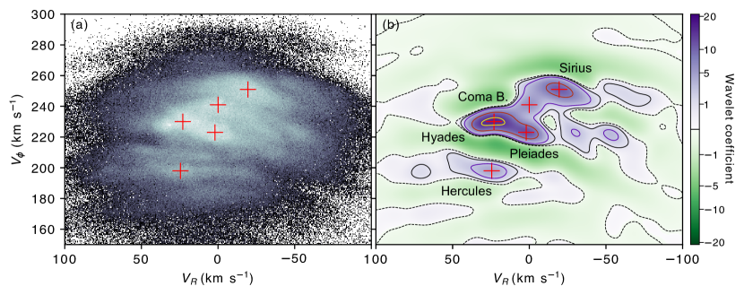
Figure 1: Panel a shows the 2D histogram of all the solar neighborhood stars in the $V_{R}-V_{\phi}$ kinematic plane using Gaia DR3 with a bin size of 0.5 km s^-1. Panel b shows the resultant wavelet transformed image at a scale of 8-16 km s^-1. The purple and green regions depict the relative strength of the positive and negative wavelet coefficients, respectively. Contours are shown at the -0.1% (dashed), 5%, 15%, 50%, and 90% levels. The red markers denote the locations of the five major moving groups as detected by our wavelet transformation – Hyades, Pleiades, Coma Berenices, Sirius, and Hercules.

An additional constraint on the properties of the MW’s nonaxisymmetric features came from the motions (in full 3D) of the stars near the Sun (e.g. Dehnen, 1998; Antoja et al., 2012). How these stars cluster in velocity space (moving groups) contains a wealth of information about the evolution of our Galaxy’s disk and the forces these stars are feeling. Specifically, the bimodality in the Galactocentric azimuthal velocity versus radial velocity plot has been one of the main features models have attempted to reproduce. The main mode (at $V_{\phi}\sim 230$ km s^-1) contains the moving groups of Hyades, Pleiades, Coma Berenices, and Sirius, while Hercules (at $V_{\phi}\sim 200$ km s^-1) is separated by a gap (a strong underdensity).

This bimodality has been explained through resonances of the MW’s bar. Since the bar contributes a nonaxisymmetric gravitational potential, it has an associated pattern speed, as discussed above. Over time, the bar perturbs the stars to align the frequencies of the stellar orbits with the bar’s frequency. These stars are “in resonance” with the bar. A bar’s strongest resonances are the corotation resonance (CR; in which the stellar and bar frequencies match exactly), and the inner and outer Lindblad resonances (ILR and OLR; in which the star completes two radial oscillations for every orbit around the galaxy). Unfortunately, both proposed models of the Galactic bar can produce this bimodality through different resonances. For a short bar, the OLR falls just inside the solar neighborhood and is able to trap stars to form Hercules (Dehnen, 2000; Fragkoudi et al., 2019). For a long bar, the CR is able to create Hercules through stars orbiting the bar’s Lagrange points (Pérez-Villegas et al., 2017; D’Onghia & L. Aguerri, 2020). Both models agree with the observations near the Sun, however as we move throughout the Galactic disk their predictions change.

With Gaia’s latest data release (Data Release 3; Gaia Collaboration et al. 2016, 2018; Gaia Collaboration et al. 2022a), we can finally begin to differentiate between these two models by looking at full 3D stellar motions across the Galactic disk. In this paper, we explore how Hercules changes as we move around the disk in azimuth, breaking the degeneracy between these two models for the MW’s bar.

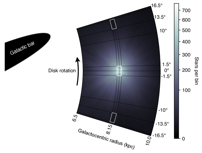
Figure 2: Gaia DR3 dataset in the context of the MW disk. This region extends from Galactocentric radius $R=6.5$ kpc to $R=10$ kpc, and from median azimuth $\phi=-15^{\circ}$ to $\phi=15^{\circ}$. An approximation of the Galactic bar is also shown. The MW disk is rotating counter-clockwise (in the direction of $+\phi$), and the solar neighborhood is trailing behind the major axis of the bar. The white boxes also show the size of our neighborhood regions, extending 0.2 kpc in $R$ and $3^{\circ}$ in $\phi$.

2 Methods

We follow the methods outlined in Lucchini et al. (2023) (hereafter Paper I) for Gaia selection and analysis using the wavelet transformation. Figure 1 shows the solar neighborhood velocity plane and its corresponding wavelet transformed image. The red marks denote the five most significant classical moving groups as detected by local maxima in the wavelet image. Starting with the 33,653,049 stars with radial velocities and geometric distances computed by Bailer-Jones et al. (2021) (Bailer-Jones et al., 2020), we transformed the six-dimensional data into Galactocentric cylindrical coordinates. See Figure 2 for a schematic defining our coordinate system with $R$ increasing away from the Galactic center, $\phi$ increasing in the direction of rotation, and $Z$ increasing towards the Galactic north pole. With the Sun located at $\phi_{\odot}=0^{\circ}$, this means the major axis of the Milky Way’s bar is at $\phi\sim 20^{\circ}$ (Gaia Collaboration et al., 2022b). Figure 2 also shows the extent of the Gaia DR3 data that we used: $6.5<R<10$ kpc, and $-15^{\circ}<\phi<15^{\circ}$. As in Paper I, we used the pyia code to propagate the errors (including correlations) from the source properties (right ascension, declination, proper motions, and radial velocities) to the final properties (Galactocentric cylindrical coordinates; Price-Whelan 2018).

For the analysis of Hercules in this paper, we broke up this region into 31 overlapping bins in $\phi$ of size $\phi=3^{\circ}$, $R=0.2$ kpc, and $Z=1$ kpc, centered on $R=8.15$ kpc and $Z=0$, spaced every $1^{\circ}$ (e.g. ranges of $(-16.5^{\circ},-13.5^{\circ})$, $(-15.5^{\circ},-12.5^{\circ})$, etc). The solar neighborhood bin contains nearly $10^{6}$ stars, while the bins at the edge of our sample ($\pm 15^{\circ}$) contain more than $10^{4}$ stars.

We use the wavelet transform code, MGwave (described in Paper I), to analyze the velocity distributions of these different neighborhoods. Each velocity plane histogram ($V_{R}-V_{\phi}$) is transformed using the Starlet transform (Starck & Murtagh, 1994; Starck & Pierre, 1998; Starck & Murtagh, 2006) and the relative significance of the results are evaluated with respect to Poisson noise (Slezak et al., 1993) and errors in the source Gaia data (using Monte Carlo simulations). In this paper, we used a wavelet scale of 8-16 km s^-1 to best identify the Hercules group. See Paper I for more details on the wavelet code and methodology.

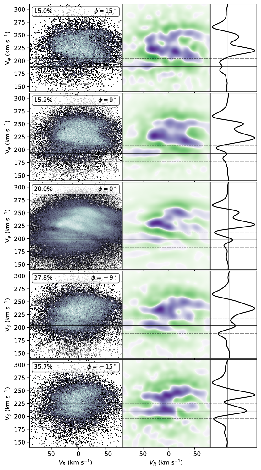
Figure 3: The velocity plane and its wavelet transformation for five neighborhoods located at $\phi=-15^{\circ}$, $-9^{\circ}$, $0^{\circ}$, $9^{\circ}$, and $15^{\circ}$. $\phi=0^{\circ}$ corresponds to the location of the Sun, and positive $\phi$ is in the direction of rotation, while negative $\phi$ is counter to the direction of rotation. The left column shows the $V_{R}-V_{\phi}$ histogram for each region, the center column shows the wavelet transformed kinematic plane as in Figure 1, and the right column shows the wavelet histogram summed along $V_{R}$. In the left column, the number of bins in the histogram has been scaled to the total number of stars such that we use 200 bins in each dimension at $\phi=\pm 15^{\circ}$, and we use 600 bins at $\phi=0^{\circ}$. Hercules is denoted by a horizontal line across each plot in a row, identified as a peak in the summed wavelet histogram (right column). Additionally, the percentage of stars that constitute Hercules (defined as all stars within 15^∘ of Hercules’ $V_{\phi}$) is printed in the top right of the left plots. In the direction of rotation (i.e. $+\phi$, towards the major axis of the MW bar) Hercules diminishes and the percentage drops, while moving towards the minor axis of the bar ($-\phi$, towards the Lagrange points) Hercules grows and merges in with the main mode. We additionally see that $V_{\phi}$ of Hercules increases as we approach the Lagrange points, as predicted by models (D’Onghia & L. Aguerri 2020; Monari et al. 2019b; see also Figure 4a).

3 Results

We track Hercules across the Galactic disk using Gaia DR3. In particular, we are looking for variations in the size and strength of the Hercules moving group as we vary the azimuth. Figure 3 shows the velocity plane for five different neighborhoods: $\phi=\pm 15^{\circ}$, $\pm 9^{\circ}$, and $0^{\circ}$ (corresponding to the solar neighborhood shown in Figure 1). These angles were chosen to show the full extent of usable data from Gaia DR3 ($\pm 15^{\circ}$, where the number of stars per bin reaches $\sim 10^{4}$), while showing an intermediate region in which Hercules is just beginning to merge with the main mode ($-9^{\circ}$). The upper panels are towards the major axis of the bar ($+\phi$), and the lower panels are towards the minor axis of the bar ($-\phi$). The left column shows the $V_{R}-V_{\phi}$ histogram of all the stars in the specified neighborhood. The center column shows the wavelet transform of these data in which purple represents overdensities and green represents underdensities (as in Figure 1). The right-most column shows a plot of wavelet coefficient as a function of $V_{\phi}$ obtained by summing the wavelet transformed image along $V_{R}$ (the “1D summed wavelet histogram”). From these plots, we are able to clearly see the location of Hercules in each neighborhood as the peak in this histogram around $V_{\phi}\sim 200$ km s^-1.

Figure 4 summarizes the properties of Hercules as a function of azimuth. Figure 4a shows the azimuthal velocity of Hercules as a function of $\phi$. This is identified by the location of the peak in the 1D summed wavelet histogram (right panels in Figure 3). A linear fit to $V_{\phi}$ of Hercules versus azimuth gives $V_{\phi\mathrm{,Herc}}=-0.74\,\phi+198$ (with $V_{\phi\mathrm{,Herc}}$ in km s^-1and $\phi$ in degrees) decreasing from 211 km s^-1at $\phi=-15^{\circ}$ to 190 km s^-1at $\phi=+15^{\circ}$. Figure 4b shows the strength of the Hercules overdensity relative to the main mode. This is measured by the value of the peak in the 1D summed wavelet histogram corresponding to Hercules. A larger value means that the overdensity is stronger. In Figure 3c, we also show the percentage of stars that constitute Hercules in each neighborhood. This is determined by selecting all the stars within $\pm 15$ km s^-1of the $V_{\phi}$ of Hercules (Figure 4a) and dividing by the total number of stars in the given bin. Examples of this 30 km s^-1region are shown bounded by the dashed horizontal lines in Figure 3. In the solar neighborhood, Hercules constitutes 20.0% of stars. As we move towards the bar’s major axis (upwards in Figure 3), this percentage decreases to 15.0% at $\phi=15^{\circ}$. As we move towards the bar’s minor axis (downwards in Figure 3), this percentage increases to 35.7% at $\phi=-15^{\circ}$.

If Hercules was formed through interaction with the Galactic bar’s outer Lindblad resonance, we would expect its strength to be relatively constant across azimuth (see Figure 12, left panel, in Fragkoudi et al. 2019). However, if the corotation resonance is responsible for Hercules, its member stars would be orbiting around the Galactic bar’s L4/L5 Lagrange points (Pérez-Villegas et al., 2017; D’Onghia & L. Aguerri, 2020) located along the bar’s minor axis. Therefore, we should expect to see a larger population of stars in Hercules as we approach L4/L5 (in the $-\phi$ direction; see Figure 4 from D’Onghia & L. Aguerri 2020). The behavior identified here in Gaia DR3, mimics exactly the predictions of D’Onghia & L. Aguerri (2020) (see their Figure 8). Along the bar’s major axis, Hercules diminishes (for both the fast and slow bar scenarios). However, along the minor axis, we are able to discriminate between these two models. For the short, fast bar, Hercules should remain subdominant and separated from the main mode. While in the long, slow bar model, Hercules should become extremely prominent, even merging with the main mode, which is what we see in the data.

Figures 4b and c show that Hercules increases in strength and fraction as we move towards the bar’s minor axis ($-\phi$). Figure 4c also shows the fraction of stars within 175$-$205 km s^-1at $R=12$ kpc (corresponding to $R/R_{\mathrm{OLR}}=0.9$, as in Dehnen 2000) to show the angular dependence due to the OLR. As expected, the fraction of stars trapped by the OLR (at $R=12$ kpc) is relatively constant in azimuth, while at the solar radius, there is a sharp increase in the $-\phi$ direction, indicating that Hercules is comprised of stars trapped at the Lagrange points.

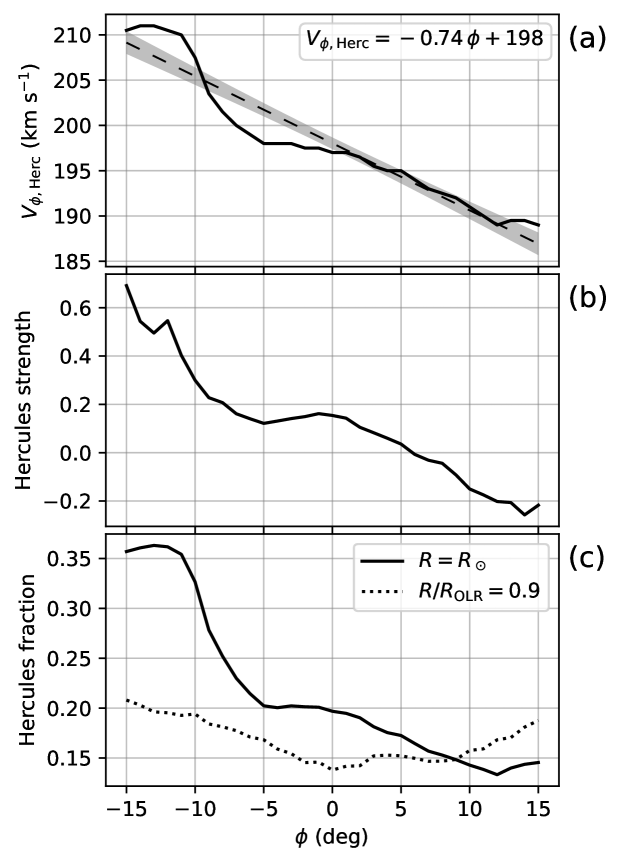
Figure 4: Properties of Hercules as a function of azimuth. The top panel shows the mean $V_{\phi}$ for the Hercules group as detected using the location of the peak in the wavelet histogram. A linear fit with the 95% confidence interval is shown as a dashed line and grey shading. The best fit equation is shown in the top right. The middle panel shows the relative strength of the Hercules overdensity normalized against the strength of the main mode. This is the value of the peak in the summed 1D wavelet histogram (see right panels in Figure 3). The bottom panel shows the percentage of stars in the given neighborhood that have $V_{\phi}$ values within 15 km s^-1of Hercules. The dotted line shows the percentage of stars within 175$-$205 km s^-1at $R=12$ kpc (such that $R/R_{\mathrm{OLR}}=0.9$, as in Dehnen 2000). At the OLR, we see no variation in intensity as a function of $\phi$. These three plots clearly show that in the $-\phi$ direction (towards the bar’s minor axis), Hercules sees an increase in angular momentum and becomes stronger and more dominant as predicted by the long, slow bar model (D’Onghia & L. Aguerri, 2020).

Moreover, as shown in Monari et al. (2019b), we would expect the angular momentum of Hercules to vary with azimuth. Figure 3 shows that the Hercules overdensity in the data changes its value of $V_{\phi}$ with angle decreasing from $V_{\phi}=211$ km s^-1at $\phi=-15^{\circ}$, to $V_{\phi}=190$ km s^-1at $\phi=+15^{\circ}$. Monari et al. (2019b) predicted a slope of $-0.96$ km s^-1deg^-1, whereas here the data show a slope of $-0.74\pm 0.04$ km s^-1deg^-1. This difference could be due to additional effects of spiral arms not included in the model of Monari et al. (2019b). However, it is clear that the slope is $<0$, consistent with Hercules being formed by corotation, not the OLR.

4 Conclusions

Here we have used Gaia DR3 to track the properties of Hercules through Galactic azimuth. Exploring $-15^{\circ}<\phi<15^{\circ}$ either side of the Sun, we see that there is a strong variation in the azimuthal velocity and strength of Hercules. Hercules becomes stronger and constitutes a larger fraction of stars per bin as we move towards the minor axis of the bar ($-\phi$). This is in direct agreement with predictions of a long, slow bar model in which Hercules is formed through stars trapped at corotation, orbiting the L4/L5 Lagrange points. This corroborates recent direct observations of the bar from Gaia DR3 (Gaia Collaboration et al., 2022b).

With the next release from Gaia, DR4, we can expect further significant improvements using this technique. While DR3 extended our view out to $\phi=\pm 15^{\circ}$, we can hope to get similar signal to noise results out to $\phi=\pm 30^{\circ}$ and beyond. This will allow us to get a direct measurement of the bar angle with respect to the Sun’s position, by looking for a minimum in Hercules’ strength and $V_{\phi}$.

Data Availability

The data underlying this article will be shared on reasonable request to the corresponding author.

References

- Antoja et al. (2012) Antoja T., et al., 2012, MNRAS, 426, L1
- Asano et al. (2020) Asano T., Fujii M. S., Baba J., Bédorf J., Sellentin E., Portegies Zwart S., 2020, MNRAS, 499, 2416
- Astropy Collaboration et al. (2013) Astropy Collaboration et al., 2013, A&A, 558, A33
- Astropy Collaboration et al. (2018) Astropy Collaboration et al., 2018, AJ, 156, 123
- Astropy Collaboration et al. (2022) Astropy Collaboration et al., 2022, apj, 935, 167
- Bailer-Jones et al. (2020) Bailer-Jones C., Rybizki J., Fouesneau M., Demleitner M., Andrae R., 2020, Gaia eDR3 lite distances subset, VO resource provided by the GAVO Data Center, http://dc.zah.uni-heidelberg.de/tableinfo/gedr3dist.litewithdist
- Bailer-Jones et al. (2021) Bailer-Jones C. A. L., Rybizki J., Fouesneau M., Demleitner M., Andrae R., 2021, AJ, 161, 147
- Benjamin et al. (2005) Benjamin R. A., et al., 2005, ApJ Letters, 630, L149
- Bovy et al. (2019) Bovy J., Leung H. W., Hunt J. A. S., Mackereth J. T., García-Hernández D. A., Roman-Lopes A., 2019, MNRAS, 490, 4740
- Clarke et al. (2019) Clarke J. P., Wegg C., Gerhard O., Smith L. C., Lucas P. W., Wylie S. M., 2019, MNRAS, 489, 3519
- D’Onghia & L. Aguerri (2020) D’Onghia E., L. Aguerri J. A., 2020, ApJ, 890, 117
- Debattista et al. (2002) Debattista V. P., Gerhard O., Sevenster M. N., 2002, MNRAS, 334, 355
- Dehnen (1998) Dehnen W., 1998, AJ, 115, 2384
- Dehnen (2000) Dehnen W., 2000, AJ, 119, 800
- Englmaier & Gerhard (1997) Englmaier P., Gerhard O., 1997, MNRAS, 287, 57
- Fragkoudi et al. (2019) Fragkoudi F., et al., 2019, MNRAS, 488, 3324
- Fux (1999) Fux R., 1999, A&A, 345, 787
- Gaia Collaboration et al. (2016) Gaia Collaboration et al., 2016, A&A, 595, A1
- Gaia Collaboration et al. (2018) Gaia Collaboration et al., 2018, A&A, 616, A11
- Gaia Collaboration et al. (2022a) Gaia Collaboration Vallenari A., Brown A., Prusti T., 2022a, A&A
- Gaia Collaboration et al. (2022b) Gaia Collaboration Drimmel R., Romero-Gómez M., Chemin L., Ramos P., Poggio E., Ripepi V., 2022b, arXiv e-prints, p. arXiv:2206.06207
- Lucchini et al. (2023) Lucchini S., Pellett E., D’Onghia E., Aguerri J. A. L., 2023, MNRAS, 519, 432
- Monari et al. (2017) Monari G., Kawata D., Hunt J. A. S., Famaey B., 2017, MNRAS, 466, L113
- Monari et al. (2019a) Monari G., Famaey B., Siebert A., Wegg C., Gerhard O., 2019a, A&A, 626, A41
- Monari et al. (2019b) Monari G., Famaey B., Siebert A., Bienaymé O., Ibata R., Wegg C., Gerhard O., 2019b, A&A, 632, A107
- Pérez-Villegas et al. (2017) Pérez-Villegas A., Portail M., Wegg C., Gerhard O., 2017, ApJ Letters, 840, L2
- Price-Whelan (2018) Price-Whelan A., 2018, adrn/pyia: v0.2, doi:10.5281/zenodo.1228136, https://doi.org/10.5281/zenodo.1228136
- Sanders et al. (2019) Sanders J. L., Smith L., Evans N. W., 2019, MNRAS, 488, 4552
- Slezak et al. (1993) Slezak E., de Lapparent V., Bijaoui A., 1993, ApJ, 409, 517
- Sormani et al. (2015) Sormani M. C., Binney J., Magorrian J., 2015, MNRAS, 454, 1818
- Starck & Murtagh (1994) Starck J.-L., Murtagh F., 1994, A&A, 288, 342
- Starck & Murtagh (2006) Starck J.-L., Murtagh F., 2006, Astronomical Image and Data Analysis (Astronomy and Astrophysics Library). Springer-Verlag, Berlin, Heidelberg
- Starck & Pierre (1998) Starck J. L., Pierre M., 1998, A&A Supplement, 128, 397
- Tremaine & Weinberg (1984) Tremaine S., Weinberg M. D., 1984, ApJ Letters, 282, L5
- Wegg et al. (2015) Wegg C., Gerhard O., Portail M., 2015, MNRAS, 450, 4050