Error Analysis of Kernel/GP Methods for Nonlinear and Parametric PDEs

Abstract

We introduce a priori Sobolev-space error estimates for the solution of nonlinear, and possibly parametric, PDEs using Gaussian process and kernel based methods. The primary assumptions are: (1) a continuous embedding of the reproducing kernel Hilbert space of the kernel into a Sobolev space of sufficient regularity; and (2) the stability of the differential operator and the solution map of the PDE between corresponding Sobolev spaces. The proof is articulated around Sobolev norm error estimates for kernel interpolants and relies on the minimizing norm property of the solution. The error estimates demonstrate dimension-benign convergence rates if the solution space of the PDE is smooth enough. We illustrate these points with applications to high-dimensional nonlinear elliptic PDEs and parametric PDEs. Although some recent machine learning methods have been presented as breaking the curse of dimensionality in solving high-dimensional PDEs, our analysis suggests a more nuanced picture: there is a trade-off between the regularity of the solution and the presence of the curse of dimensionality. Therefore, our results are in line with the understanding that the curse is absent when the solution is regular enough.

60G15, 65M75, 65N75, 65N35, 47B34, 41A15, 35R30, 34B15.

1 Introduction

In recent years the adoption of machine learning in the natural sciences and engineering has led to the development of new methods for solving PDEs [65, 79, 80, 44, 47]. The majority of these methods rely on the approximation power of artificial neural networks (ANNs) either as a function class to approximate the solution of the PDE or as a high-dimensional function class to approximate the solution map of the PDE. Despite the empirical success of the aforementioned ANN based methods, current theoretical understanding of these PDE solvers is scarce and, beyond particular PDEs (e.g., [74, 48, 24]), results are oftentimes limited to existence results rather than convergence guarantees or rates.

Similar to ANNs, kernel methods and Gaussian processes (GPs) have been very effective in scientific computing and machine learning [73, 54, 6, 82] and at the same time they are supported by rigorous theoretical foundation [6, 81, 61]. Recently in [11], the authors introduced a kernel collocation method for solving arbitrary nonlinear PDEs with a rigorous convergence guarantee. The theory presented in that work was based on the assumptions that (1) the solution belongs to the reproducing kernel Hilbert space (RKHS) defined by the underlying kernel which in turn is embedded in the Sobolev space $H^{s}$ for $s>d/2\>+$“order of the PDE” (where $d$ is the dimension of the domain of the PDE) and (2) the fill-distance between collocation points goes to zero. Convergence was proved via a compactness argument but no convergence rates were provided.

The goal of this article is to provide quantitative convergence rates for the PDE solver introduced in [11]. Our quantitaitve rates also reveal the interplay between the regularity of the solution of the PDE and the dimension $d$ of the problem. At the same time we make improvements to the methodology of [11] and extend it to the case of parametric PDEs. In the rest of this section we summarize our main contributions in Section 1.1 followed by a review of the relevant literature in Section 1.2, and an outline of the article in Section 1.4.

1.1 Our Contributions

Throughout the article we consider parametric PDEs of the form

(1) $$\left\{\begin{aligned} \mathcal{P}(u^{\star})(\mathbf{x};\bm{\theta})&=f(\mathbf{x};\bm{\theta}),&&(\mathbf{x},\bm{\theta})\in\Omega\times\Theta,\\ \mathcal{B}(u^{\star})(\mathbf{x};\bm{\theta})&=g(\mathbf{x};\bm{\theta}),&&(\mathbf{x},\bm{\theta})\in\partial\Omega\times\Theta,\end{aligned}\right.$$

where $\Omega\subset\mathbb{R}^{d}$ is a bounded connected domain with an appropriately smooth boundary $\partial\Omega$, $\mathcal{P}$ and $\mathcal{B}$ are the interior and boundary differential operators that define the PDE and $f,g$ are the source and boundary data. $\mathbf{x}$ denotes the spatial variable with $\bm{\theta}$ denoting a parameter belonging to a compact set $\Theta\subset\mathbb{R}^{p}$. The function $u^{\star}$ denotes the exact, strong solution of this PDE.

We view the solution $u^{\star}$ as a function on $\overline{\Omega}\times\Theta$ and approximate it in an appropriate RKHS by imposing the PDE as a constraint on a set of collocation points in the product space $\overline{\Omega}\times\Theta$. Our main contributions are three-fold as summarized below:

1. We extend the kernel PDE solver of [11] to the case of the parametric PDE (1). This extension follows by viewing the solution $u^{\star}(\mathbf{x};\theta)$ as a continuous function defined on $\overline{\Omega}\times\Theta$ and approximating it with a function $u^{\dagger}$ in an appropriate RKHS $\mathcal{U}$ after imposing the PDE as a constraint on a set of collocation points. At the same time we improve the efficacy and performance of the Gauss-Newton (GN) algorithm of [11] through an approach of “linearize first then apply the kernel solver”. For many prototypical PDEs this new approach leads to smaller kernel matrices that can be factored or inverted more efficiently. These numerical strategies are outlined in Section 2.

2. We provide explicit a priori convergence rates for the kernel estimator $u^{\dagger}\in\mathcal{U}$ to the true solution $u^{\star}$. Our proof relies on three assumptions: (1) the RKHS $\mathcal{U}\subset H^{s}(\Omega)$ for $s>(d+p)/2+\text{``order of the PDE''}$; (2) the true unique solution $u^{\star}\in\mathcal{U}$; (3) the forward PDE operator and the associated solution map of the PDE are Lipschitz stable. Our error estimates are of the general form

   (2) $$\|u^{\dagger}-u^{\star}\|_{L^{2}(\Omega)}\lesssim h^{s}\|u^{\star}\|_{\mathcal{U}},$$

   where $h$ is the fill-distance (mesh-norm) of our collocation points. Indeed, if expressed in terms of $N$, the number of collocation points, the rate will read as $\mathcal{O}(N^{-s/(d+p)})$. The above rate indicates a trade-off between the regularity of the solution space and the dimension $d+p$ of $\Omega\times\Theta$ stating that the convergence rate is dimension-benign so long as the solution $u^{\star}$ is sufficiently regular; these results are outlined in Section 3.

3. In fact, our method for proving the rate (2) is more general than the case of PDEs (see Figure 1 for the road map of the proof technique). The proof can be viewed as a recipe for convergence analysis of solutions to nonlinear functional equations of the form $\mathcal{P}(u)=f$ where $u,f$ belong to sufficiently regular function spaces and $\mathcal{P}$ is invertible (at least locally). Then the Lipschitz stability of $\mathcal{P}$ and $\mathcal{P}^{-1}$ plus RKHS interpolation bounds on $f$ yield convergence rates for $u$. Results at this level of generality are presented in [69] for linear maps $\mathcal{P}$ which are then extended to nonlinear problems in [8, 9]. In these works, the stability of the discretization method is furthermore assumed. In the GP methodology, this property is guaranteed, due to the minimal RKHS norm property of the solution. This has been pointed out in [69, Sec. 10] for linear PDEs. Our theory can be seen as a generalization of the result in [69] to the nonlinear case.

4. We present a suite of numerical experiments that elucidate and extend our theoretical analysis in item 2. We present an example of a nonlinear elliptic PDE with a prescribed solution of varying regularity in various dimensions. We then explore the interplay between regularity and dimensionality as well as the rate in (2). We further verify our result for a one dimensional parametric PDE by varying $p$, the dimension of the parameter space $\Theta$. Because of this trade-off between regularity and dimensionality, showing that a numerical method remains accurate for a high dimensional PDE may not be an indication that it is breaking the curse of dimensionality but simply an indication that the problem being solved is very regular; see our experiments in Section 4 and in particular Section 4.3.

Figure 1: A summary of the main steps in our proof of convergence rates outlined in Theorems 3.1, 3.3, 3.8, and 3.12. The 1–4 norms denote arbitrary norms on appropriate Banach spaces while the $\|\cdot\|_{\mathcal{U}}$-norm can be chosen as an RKHS norm or another desired norm with respect to which the numerical algorithm is stable.

1.2 Relevant Literature

Below we present a brief review of the relevant literature to the current work.

1.2.1 Kernel and Gaussian Process Solvers for PDEs

As mentioned earlier our algorithmic and theoretical developments are focused on the kernel method introduced in [11] and extending that approach to parametric PDEs. Further extensions and applications of the aforementioned framework can also be found in [53, 52, 45, 12]. When applied to linear PDEs our kernel method coincides with the so-called symmetric collocation method [70, Sec. 14] and is closely associated with radial basis function (RBF) PDE solvers [26, 28]. Various error analyses for RBF collocation methods can be found in [27, 28]. In particular, the article [31] is the closest to our work and their rates coincide with ours in the linear PDE setting. The article [14] presents similar bounds for the so-called Kansa method [36, 37], a non-symmetric RBF collocation PDE solver. Finally, [69] presents an abstract set of convergence rates for RBF interpolation of “well-posed” linear maps between regular function spaces that includes RBF PDE solvers as a special case. All of the aforementioned analyses consider linear PDEs and some generalizations to nonlinear problems are studied in [8, 9].

The deep connection of Kernels and RKHSs to the theory of GPs [7, 40, 82, 77] suggests that kernel PDE solvers can be viewed from lens of probability theory as a conditioning problem for GPs. While not as extensively developed as the kernel solvers mentioned earlier, this direction has been explored for the solution of linear PDEs as well as nonlinear ODEs [17, 20, 59, 68, 75] and recent works have extended this idea to some nonlinear and time-dependent PDEs [19, 64, 78]. The GP interpretation is attractive due to the ability to provide rigorous uncertainty estimates along with the solution to the PDE. The idea here is that the uncertainties can serve as a posterior or a priori error indicators for the PDE solver. Some ideas related to this direction were discussed in [11, 19]. A fully probabilistic GP interpretation of our kernel framework for linear PDEs can be found in [59, 19, 61] but the case of nonlinear PDEs remains partially investigated [11, 52, 53, 46]. Moreover we note that in the GP framework, hierarchical Bayes learning can be used to select kernels to get better convergence rates [13, 83, 62, 23].

1.2.2 Parametric and High-dimensional PDEs

Parametric PDEs are ubiquitous is physical sciences and engineering and in particular in the context of uncertainty quantification (UQ) and solution of stochastic PDEs (SPDEs) [18, 30, 41, 85]. A vast literature exists on the subject, connecting it to reduced basis models [1, 58], emulation of computer codes [39], reduced order models [49], and numerical homogenization [61]; for settings that most closely resemble our problems we refer the reader to [30, 84, 21] for a general overview. Broadly speaking, the dominant approaches for approximation of high-dimensional and parametric solution maps include polynomial/Taylor approximation methods [5, 15, 16, 57, 56]; Galerkin methods [34, 22]; reduced basis methods [35]; and more recently ANN operator learning techniques such as [44, 47]. In comparison to the aforementioned works we propose to directly approximate the solution of the parametric PDE as a function on the tensor product space of the physical and parameter domains in a similar spirit as [38]. The recent article [4] also presents a kernel based operator learning approach to various PDE problems including parametric PDEs.

1.2.3 The Curse of Dimensionality

Although the trade-off between regularity and accuracy is well understood in numerical approximation/integration, where it has led to the development of the Kolmogorov $N$-width and stress tests for finite-element methods [63, 51, 3], its impact is oftentimes overlooked when communicating the convergence of Machine Learning and Deep Learning methods for high-dimensional PDEs. In particular, since artificial neural networks (ANNs) can be interpreted as kernel methods [55, 42, 60] with data-dependent parameterized kernels, our results raise the further question of understanding whether the (empirically observed) convergence of ANN-based methods for high-dimensional PDEs is an indication of the absence of the curse (i.e., the regularity of the solution in selected numerical experiments is high) or the breaking of that curse. In particular, empirically observing numerical accuracy for an algorithm and particular solutions is insufficient to prove that the curse of dimensionality is broken, and one must also show that the underlying problem and those solutions are not too regular. We emphasize that the curse of dimensionality referred to here, is the one associated with the worsening of the accuracy of a numerical approximation algorithm as a function of the dimension of the domain of the PDE as opposed to the impact of the curse on the number of degrees of freedom in the implementation level (e.g., finite difference methods suffer from that second curse but ANN/kernel based methods do not).

1.3 On the Importance of Developing and Benchmarking against Kernel/GP Methods

The proposed work aims to further develop Gaussian Process (GP) and kernel methods for solving PDEs. We are motivated to do so because GP methods have the potential to offer the best of both worlds by combining the strengths and flexibility of traditional and Deep Learning (DL) methods while also being equipped with theoretical guarantees and uncertainty quantification (UQ) capabilities.

Compared to traditional methods (such as finite element methods (FEM), finite volume methods (FVM), finite difference methods (FDM), spectral methods, etc), GP methods generalize meshless, RBF, optimal recovery methods and are flexible and applicable in high dimensions. Compared to DL methods that use an expressive neural network representation, GPs offer transparent methods that are easy to reproduce and analyze. Furthermore the natural probabilistic interpretation of GPs enables convenient UQ and also facilitates the process of scientific discovery itself [61]; FEM and DL methods do not interface so cleanly with UQ. Moreover, with hierarchical kernel learning [13, 83, 62, 23], GP methods can also be made highly expressive. In fact, as shown in the table below, GP methods can offer many advantages over traditional and DL methods. In the context of PDEs these advantages include: greater flexibility, applicability in high dimensions, provable guarantees, near-linear complexity computation, Occam’s razor principle in the design of statistical models, mathematical transparency and interpretability, and ease of reproducibility; see Table 1. Although software support for GPs is currently not as advanced as that for DL and traditional methods, GPs are still easy to program and can be seamlessly integrated into an engineering pipeline.

Method	Ease of implementation in high-dimensions	Provable guarantees	Near linear complexity	Occam’s razor	Transparent	Ease of reproducibility	Built-in UQ	Software support
Trad.	✗	✓	✓	✓	✓	✓	✗	✓
Kernel	✓	✓	✓	✓	✓	✓	✓	Limited
ANN	✓	Limited	✗	✗	✗	Limited	✗	✓

Table 1: A qualitative comparison of the properties of traditional PDE solvers (such as FEM, FVM, FDM, spectral methods, etc) against kernel methods and ANNs.

Given their long training times, ANN-based methods may not be competitive with FEM in low dimensions [33]. In contrast, GP-based methods can achieve near-linear complexity when combined with fast algorithms for kernel methods such as the sparse Cholesky factorization [71, 72, 12]. In some applications, these algorithms can be competitive (both in terms of complexity and accuracy) even when compared to highly optimized algebraic multigrid solvers such as AMGCL and Trilinos [10]. GP methods are naturally amenable to analysis and come with simple provable guarantees, while ANN-based methods involve complicated optimizations and many heuristics, which can make them hard to understand. GP methods fit Occam’s razor, offering a clarity of purpose in their structure. We can understand why and when they work, which is of scientific importance [25]. Therefore, it is increasingly important to benchmark deep learning methods against kernel-based methods to ensure that the deep part of a DL method serves a significant purpose beyond adding complexity.

1.4 Outline of the Article

The rest of the article is organized as follows: We present a brief overview of our GP and kernel approach for solving nonlinear and parametric PDEs in Section 2; our error analysis is outlined in Section 3; followed by numerical experiments in Section 4 and conclusions in Section 5. Auxiliary results are collected in Appendices A, B, and C.

2 Kernel Methods for Parametric PDEs

In this section we extend the kernel methodology of [11] to the case of parametric PDEs as outlined in Section 2.1. Some numerical strategies and ideas for improving the efficiency of the solver are discussed in Section 2.2.

2.1 Solving Parametric PDEs

Let us consider bounded connected domains $\Omega\in\mathbb{R}^{d}$ with a Lipschitz boundary for $d\geq 1$ and $\Theta\subset\mathbb{R}^{p}$ for $p\geq 1$. We consider nonlinear and parametric PDEs of the form

(3) $$\left\{\begin{aligned} \mathcal{P}(u^{\star})(\mathbf{x};\bm{\theta})&=f(\mathbf{x};\bm{\theta}),&&(\mathbf{x},\bm{\theta})\in\Omega\times\Theta,\\ \mathcal{B}(u^{\star})(\mathbf{x};\bm{\theta})&=g(\mathbf{x};\bm{\theta}),&&(\mathbf{x},\bm{\theta})\in\partial\Omega\times\Theta,\end{aligned}\right.$$

where $\mathcal{P},\mathcal{B}$ are nonlinear differential operators in the interior and boundary of $\Omega$, $\bm{\theta}$ is a parameter, and $f,g$ are the PDE source and boundary data. For now we assume that the above PDE is well-posed and has a unique solution $u^{\star}(\mathbf{x};\bm{\theta})$ which is assumed to exist in the strong sense over $\overline{\Omega}$ and for all values of $\bm{\theta}\in\Theta$. In [11] the authors introduced a GP/kernel method for solving nonlinear PDEs of the form (3) without parametric dependence. Here we extend that approach to the parametric case.

Let $\Upsilon:=\Omega\times\Theta$ and $\partial\Upsilon:=\partial\Omega\times\Theta$ and write $\mathbf{s}:=(\mathbf{x},\bm{\theta})$. Choose $M\geq 1$ collocation points $\{\mathbf{s}_{m}\}_{m=1}^{M}\in\overline{\Upsilon}$ such that $\{\mathbf{s}_{m}\}_{m=1}^{M_{\Omega}}\in\Upsilon$ and $\{\mathbf{s}_{m}\}_{m=M_{\Omega}+1}^{M}\in\partial\Upsilon$ and consider a kernel $K:\overline{\Upsilon}\times\overline{\Upsilon}\to\mathbb{R}$ with its corresponding RKHS denoted by $\mathcal{U}$ and norm $\|\cdot\|_{\mathcal{U}}$. We then propose to approximate $u^{\star}(\mathbf{s})$ by solving the optimization problem

(4) $$\left\{\begin{aligned} \operatorname*{{\rm minimize}}_{u\in\mathcal{U}}\quad&\|u\|_{\mathcal{U}}\\ {\rm\,s.t.}\quad&\mathcal{P}(u)(\mathbf{s}_{m})=f(\mathbf{s}_{m}),&&m=1,\dots,M_{\Omega},\\ &\mathcal{B}(u)(\mathbf{s}_{m})=g(\mathbf{s}_{m}),&&m=M_{\Omega}+1,\dots,M.\end{aligned}\right.$$

Observe that our approach above approximates the solution $u$ as a function defined on the set product set $\Upsilon$ which is different from previous works [5, 15, 16, 57, 56] where the solution map $\bm{\theta}\to u^{\star}(\cdot;\bm{\theta})$, as a mapping from $\Theta$ to an appropriate function space, is characterized and approximated. The latter approach requires different discretization methods for the $\bm{\theta}$ parameter and the functions $u^{\star}(\cdot;\bm{\theta})$ while our approach leads to a meshless collocation method on the product space which is desirable and convenient at the level of implementation, following [11, Sec. 3.1] (see also [31]).

We make the following assumption on the differential operators $\mathcal{P},\mathcal{B}$. There exist bounded and linear operators $L_{1},\dots,L_{Q_{\Omega}}\in\mathcal{L}\big{(}\mathcal{U};C(\Upsilon)\big{)}$ and $L_{Q_{\Omega}+1},\dots,L_{Q}\in\mathcal{L}\big{(}\mathcal{U};C(\partial\Upsilon)\big{)}$ for some $1\leq Q_{\Omega}<Q$ together with maps $P:\mathbb{R}^{Q_{\Omega}}\to\mathbb{R}$ and $B:\mathbb{R}^{Q-Q_{\Omega}}\to\mathbb{R}$, which may be nonlinear, so that $\mathcal{P},\mathcal{B}$ can be written as

(5) $$\mathcal{P}(u)(\mathbf{s}) =P\Big{(}L_{1}(u)(\mathbf{s}),\dots,L_{Q_{\Omega}}(u)(\mathbf{s})\Big{)} \forall\mathbf{s}\in\Upsilon,$$

$$\mathcal{B}(u)(\mathbf{s}) =B\Big{(}L_{Q_{\Omega}+1}(u)(\mathbf{s}),\dots,L_{Q}(u)(\mathbf{s})\Big{)} \forall\mathbf{s}\in\partial\Upsilon.$$

$\Diamond$ We briefly introduce a running example of a parametric PDE for which the above assumptions can be verified easily.

Example 2.1 (Nonlinear Darcy flow).

Consider the nonlinear Darcy flow PDE

(6) $$\left\{\begin{aligned} -\text{div}_{\mathbf{x}}\big{(}\exp(a(\mathbf{x},\bm{\theta}))\nabla u\big{)}(\mathbf{x})+\tau(u(\mathbf{x}))&=1,&&\mathbf{x}\in\Omega,\\ u(\mathbf{x})&=0,&&\mathbf{x}\in\partial\Omega,\end{aligned}\right.$$

where $\Omega\subset\mathbb{R}^{d}$ is a bounded domain with a Lipschitz boundary and $\tau:\mathbb{R}\to\mathbb{R}$ is a continuous and nonlinear map. We assume that the permeability field $a$ is parameterized as

(7) $$a(\mathbf{x},\bm{\theta})=\sum_{j=1}^{p}\theta_{j}\psi_{j}(\mathbf{x}),$$

where $\theta_{j}\in(0,1)$ so that $\Theta=(0,1)^{p}$ and $\psi_{j}\in C(\overline{\Omega})$. Substituting into the PDE and expanding the differential operator we can rewrite our nonlinear PDE as

$$\left\{\begin{aligned} -\exp\left(\sum_{j=1}^{p}\theta_{j}\psi_{j}(\mathbf{x})\right)\sum_{j=1}^{p}\theta_{j}\nabla_{\mathbf{x}}\psi_{j}(\mathbf{x})\cdot\nabla_{\mathbf{x}}u(\mathbf{x};\bm{\theta})\hskip 43.05542pt&&&\\ -\exp\left(\sum_{j=1}^{p}\theta_{j}\psi_{j}(\mathbf{x})\right)\Delta_{\mathbf{x}}u(\mathbf{x};\bm{\theta})+\tau(u(\mathbf{x};\bm{\theta}))&=1,&&(\mathbf{x},\bm{\theta})\in\Omega\times\Theta,\\ u(\mathbf{x};\bm{\theta})&=0,&&(\mathbf{x},\bm{\theta})\in\partial\Omega\times\Theta,\end{aligned}\right.$$

where we used subscripts on the differential operators to highlight that derivatives are computed for the $\mathbf{x}$ variable only and not $\bm{\theta}$. We also did not use the compact notation $\mathbf{s}\equiv(\mathbf{x},\bm{\theta})$ since it is more helpful to be able to distinguish between the $\mathbf{x}$ and $\bm{\theta}$ variables in this example. We can directly verify Section 2.1 with the bounded and linear operators

$$L_{1} :u(\mathbf{x};\bm{\theta})\mapsto u(\mathbf{x};\bm{\theta}),$$

$$L_{2} :u(\mathbf{x};\bm{\theta})\mapsto\exp\left(\sum_{j=1}^{p}\theta_{j}\psi_{j}(\mathbf{x})\right)\sum_{j=1}^{p}\theta_{j}\nabla_{\mathbf{x}}\psi_{j}(\mathbf{x})\cdot\nabla_{\mathbf{x}}u(\mathbf{x};\bm{\theta}),$$

$$L_{3} :u(\mathbf{x};\bm{\theta})\mapsto\exp\left(\sum_{j=1}^{p}\theta_{j}\psi_{j}(\mathbf{x})\right)\Delta_{\mathbf{x}}u(\mathbf{x};\bm{\theta})$$

$$L_{4} :u(\mathbf{x};\bm{\theta})\mapsto u(\mathbf{x};\bm{\theta}),$$

Note that operators $L_{1},L_{4}$ are the same here since the point values of $u$ appear in both the interior and boundary conditions. Thus we have $Q_{\Omega}=3$ and $Q=4$ and the maps

$$P(t_{1},t_{2},t_{3})=-t_{2}-t_{3}+\tau(t_{1}),\qquad B(t_{1})=t_{1}.$$

$\Diamond$

If $\mathcal{U}$ is sufficiently regular and Section 2.1 holds, then we can define the functionals $\phi_{m}^{q}\in\mathcal{U}^{\ast}$ for $1\leq q\leq Q$ as

(8) $$\phi_{m}^{q}:=\delta_{(\mathbf{s}_{m})}\circ L_{q},\quad\text{where}\quad\left\{\begin{aligned} 1&\leq m\leq M_{\Omega}&\text{if}&&1\leq q\leq Q_{\Omega}\\ M_{\Omega}+1&\leq m\leq M&\text{if}&&Q_{\Omega+1}\leq q\leq Q.\\ \end{aligned}\right.$$

In what follows we write $[\phi,u]$ to denote the duality pairing between $\mathcal{U}$ and $\mathcal{U}^{\ast}$ and further use the shorthand notation ${\bm{\phi}}^{(q)}$ to denote the vector of dual elements $\phi^{q}_{m}$ for a fixed index $q$. Note that ${\bm{\phi}}^{(q)}\in(\mathcal{U}^{\ast})^{\otimes M_{\Omega}}$ if $q\leq Q_{\Omega}$ but ${\bm{\phi}}^{(q)}\in(\mathcal{U}^{\ast})^{\otimes(M-M_{\Omega})}$ if $q>Q_{\Omega}$ in order to accommodate different differential operators defining the PDE and the boundary conditions. We further write $N=M_{\Omega}Q_{\Omega}+(M-M_{\Omega})(Q-Q_{\Omega})$ and define

$${\bm{\phi}}=\big{(}{\bm{\phi}}^{(1)},\dots,{\bm{\phi}}^{(Q)}\big{)}\in(\mathcal{U}^{\ast})^{\otimes N}.$$

Henceforth we write $\phi_{n}$ for $n=1,\dots,N$ to denote the entries of the vector ${\bm{\phi}}$ and write $[{\bm{\phi}},u]=([\phi_{1},u],\dots,[\phi_{N},u])\in\mathbb{R}^{N}$. With this notation we rewrite problem (4) as

$$\left\{\begin{aligned} \operatorname*{{\rm minimize}}\quad&\|u\|_{\mathcal{U}}\\ {\rm\,s.t.}\quad&F([{\bm{\phi}},u])=\mathbf{y},\end{aligned}\right.$$

where the data vector $\mathbf{y}\in\mathbb{R}^{M}$ has entries

$$y_{m}:=\left\{\begin{aligned} &f(\mathbf{s}_{m}),&&\text{if}&&1\leq m\leq M_{\Omega},\\ &g(\mathbf{s}_{m}),&&\text{if}&&M_{\Omega}+1\leq m\leq M,\end{aligned}\right.$$

and $F:\mathbb{R}^{N}\to\mathbb{R}^{M}$ is a nonlinear map whose output components are defined as

(9) $$\big{(}F([{\bm{\phi}},u])\big{)}_{m}:=\left\{\begin{aligned} &P\left([\phi^{1}_{m},u],\dots,[\phi^{Q_{\Omega}}_{m},u]\right)&&\text{if }1\leq m\leq M_{\Omega},\\ &B\left([\phi^{Q_{\Omega}+1}_{m},u],\dots,[\phi^{Q}_{m},u]\right)&&\text{if }M_{\Omega}+1\leq m\leq M.\end{aligned}\right.$$

Further define the kernel vector field

(10) $$K(\cdot,{\bm{\phi}}):\overline{\Upsilon}\to\mathcal{U}^{N},\qquad K(\mathbf{s},{\bm{\phi}})_{k}:=[\phi_{k},K(\mathbf{s},\cdot)]$$

and the kernel matrix

(11) $$K({\bm{\phi}},{\bm{\phi}})\in\mathbb{R}^{N\times N},\qquad K({\bm{\phi}},{\bm{\phi}})_{nk}:=[\phi_{n},K(\cdot,{\bm{\phi}})_{k}].$$

We can then characterize the minimizers of (4) via the following representer theorem which is a direct consequence of [11, Prop. 2.3]:

Proposition 2.2.

Suppose Section 2.1 holds and $K({\bm{\phi}},{\bm{\phi}})$ is invertible. Then a function $u^{\dagger}:\overline{\Upsilon}\to\mathbb{R}$ is a minimizer of (4) if and only if

(12) $$u^{\dagger}(\mathbf{s})=K(\mathbf{s},{\bm{\phi}})K({\bm{\phi}},{\bm{\phi}})^{-1}\mathbf{z}^{\dagger},$$

where $\mathbf{z}^{\dagger}\in\mathbb{R}^{N}$ solves

(13) $$\left\{\begin{aligned} \operatorname*{{\rm minimize}}_{\mathbf{z}\in\mathbb{R}^{N}}\quad&\mathbf{z}^{T}K({\bm{\phi}},{\bm{\phi}})^{-1}\mathbf{z},\\ {\rm\,s.t.}\quad&F(\mathbf{z})=\mathbf{y},\end{aligned}\right.$$

with the nonlinear map $F$ defined in (9).

This result allows us to reduce the infinite-dimensional optimization problem (4) to a finite-dimensional optimization problem without incurring any approximation errors; it is an instance of the well-known family of representer theorems [73, Sec. 4.2]. Thus, to find an approximation to $u^{\star}$ we simply need to solve (13) and apply the formula (12); algorithms for this task are discussed next.

2.2 Numerical Strategies

We now summarize various numerical strategies for solution of (13). These strategies are naturally applicable to non-parametric PDEs as they can be viewed as a special case of (3) with a fixed parameter. In Section 2.2.1 we summarize a Gauss-Newton algorithm that was introduced in [11] followed by a new and, often, more efficient strategy that linearizes the PDE first before formulating the optimization problem in Section 2.2.2.

2.2.1 Gauss-Newton

To solve the optimization problem (13), a Gauss-Newton algorithm was proposed in [11] which we recall briefly. The equality constraints can be dealt with either by elimination or relaxation. Suppose that there exists a map $\overline{F}:\mathbb{R}^{N-M}\times\mathbb{R}^{M}\to\mathbb{R}^{N}$ so that

$$F(\mathbf{z})=\mathbf{y}\quad\text{ if and only if }\quad\mathbf{z}=\overline{F}(\mathbf{w},\mathbf{y}),\quad\text{ for a unique }\mathbf{w}\in\mathbb{R}^{N-M}\,.$$

Then, we rewrite (13) as the unconstrained optimization problem

(14) $$\operatorname*{{\rm minimize}}_{\mathbf{w}\in\mathbb{R}^{N-M}}\quad\overline{F}(\mathbf{w},\mathbf{y})^{T}K({\bm{\phi}},{\bm{\phi}})^{-1}\overline{F}(\mathbf{w},\mathbf{y})\,.$$

Then a minimizer $\mathbf{w}^{\dagger}$ of (14) can be approximated with a sequence of elements $\mathbf{w}^{\ell}$ defined iteratively via $\mathbf{w}^{\ell+1}=\mathbf{w}^{\ell}+\alpha^{\ell}\delta\mathbf{w}^{\ell},$ where $\alpha^{\ell}>0$ is an appropriate step size while $\delta\mathbf{w}^{\ell}$ is the minimizer of the optimization problem

$$\operatorname*{{\rm minimize}}_{\delta\mathbf{w}\in\mathbb{R}^{N-M}}\quad\left(\overline{F}(\mathbf{w}^{\ell},\mathbf{y})+\nabla_{\mathbf{w}}\overline{F}(\mathbf{w}^{\ell},\mathbf{y})\delta\mathbf{w}\right)^{T}K({\bm{\phi}},{\bm{\phi}})^{-1}\left(\overline{F}(\mathbf{w}^{\ell},\mathbf{y})+\nabla_{\mathbf{w}}\overline{F}(\mathbf{w}^{\ell},\mathbf{y})\delta\mathbf{w}\right)\,.$$

Alternatively, if the map $\overline{F}$ does not exist or is hard to compute, i.e., eliminating the constraints is not feasible, then we consider the relaxed problem

$$\operatorname*{{\rm minimize}}_{\mathbf{z}\in\mathbb{R}^{N}}\quad\frac{1}{2}\mathbf{z}^{T}K({\bm{\phi}},{\bm{\phi}})^{-1}\mathbf{z}+\frac{1}{2\beta^{2}}|F(\mathbf{z})-\mathbf{y}|^{2},$$

for a sufficiently small parameter $\beta>0$. Here $\|\cdot\|$ is the $L^{2}$ norm of the vector. A minimizer $\mathbf{z}^{\dagger}_{\beta}$ of the above problem can be approximated with a sequence $\mathbf{z}^{\ell}$ where $\mathbf{z}^{\ell+1}=\mathbf{z}^{\ell}+\alpha^{\ell}\delta\mathbf{z}^{\ell}$ where $\delta\mathbf{z}^{\ell}$ is the minimizer of

$$\operatorname*{{\rm minimize}}_{\delta\mathbf{z}\in\mathbb{R}^{N}}\quad\delta\mathbf{z}^{T}K({\bm{\phi}},{\bm{\phi}})^{-1}\mathbf{z}^{\ell}+\frac{1}{2\beta^{2}}|F(\mathbf{z}^{\ell})+\nabla F(\mathbf{z}^{\ell})\delta\mathbf{z}-\mathbf{y}|^{2}.$$

2.2.2 Linearize then Optimize

The Gauss-Newton approach of Section 2.2.1 is applicable to wide families of nonlinear PDEs. The primary computational bottleneck of that approach is the construction and factorization of the kernel matrix $K({\bm{\phi}},{\bm{\phi}})$ which for some PDEs can be prohibitively large. To get around this difficulty we propose an alternative approach to approximating the solution of (4) by first linearizing the PDE operators before applying Proposition 2.2. The resulting approach is more intrusive in comparison to the Gauss-Newton method as it requires explicit calculations involving the PDE but often leads to smaller kernel matrices and better performance. This method can also be viewed as applying the methodology of [11, 31] to discretize successive linearizations of the PDE.

Let $u^{\dagger}$ denote the minimizer of (4) as before. Assuming that the operators $\mathcal{P}$ and $\mathcal{B}$ are Fréchet differentiable we then approximate $u^{\dagger}$ with a sequence of elements $u^{\ell}$ obtained by solving the problem

(15) $$\left\{\begin{aligned} \operatorname*{{\rm minimize}}_{u\in\mathcal{U}}\quad&\|u\|_{\mathcal{U}}\\ {\rm\,s.t.}\quad&\left(\mathcal{P}(u^{\ell-1})+\mathcal{P}^{\prime}(u^{\ell-1})(u-u^{\ell-1})\right)|_{\mathbf{s}_{m}}=f(\mathbf{s}_{m}),&&m=1,\dots,M_{\Omega},\\ &\left(\mathcal{B}(u^{\ell-1})+\mathcal{B}^{\prime}(u^{\ell-1})(u-u^{\ell-1})\right)|_{\mathbf{s}_{m}}=g(\mathbf{s}_{m}),&&m=M_{\Omega}+1,\dots,M,\end{aligned}\right.$$

where, $\mathcal{P}^{\prime}$ and $\mathcal{B}^{\prime}$ are the Fréchet derivatives of $\mathcal{P}$ and $\mathcal{B}$.

Let us further suppose that Section 2.1 holds. Observing that the constraints in (15) are linear in $u$ we obtain an explicit formula for $u^{\ell}$ by [11, Prop. 2.2]:

(16) $$u^{\ell}(\mathbf{s})=K(\mathbf{s},\tilde{{\bm{\phi}}}^{\ell-1})K(\tilde{{\bm{\phi}}}^{\ell-1},\tilde{{\bm{\phi}}}^{\ell-1})^{-1}\mathbf{z}^{\ell-1}$$

where $\mathbf{z}^{\ell-1}=(z_{1}^{\ell-1},\dots,z^{\ell-1}_{M})^{T}$ has entries

$$z^{\ell-1}_{m}=\left\{\begin{aligned} &\left(f-\mathcal{P}(u^{\ell-1})+\mathcal{P}^{\prime}(u^{\ell-1})u^{\ell-1}\right)|_{\mathbf{s}_{m}},&&\text{if }1\leq m\leq M_{\Omega},\\ &\left(f-\mathcal{P}(u^{\ell-1})+\mathcal{B}^{\prime}(u^{\ell-1})u^{\ell-1}\right)|_{\mathbf{s}_{m}},&&\text{if }M_{\Omega}+1\leq m\leq M.\end{aligned}\right.$$

The vectors $\tilde{{\bm{\phi}}}^{\ell-1}\in(\mathcal{U}^{\ast})^{\otimes M}$ are obtained by concatenating the dual elements

$$\tilde{\phi}_{m}^{\ell-1}:=\left\{\begin{aligned} &\delta_{(\mathbf{s}_{m})}\circ\mathcal{P}^{\prime}(u^{\ell-1}),&&\text{if }m=1,\dots,M_{\Omega},\\ &\delta_{(\mathbf{s}_{m})}\circ\mathcal{B}^{\prime}(u^{\ell-1}),&&\text{if }m=M_{\Omega}+1,\dots,M.\\ \end{aligned}\right.$$

We note that the above scheme implicitly assumes that $\mathcal{U}$ is sufficiently regular so that the derivatives $\mathcal{P}^{\prime}(u^{\ell-1})$ and $\mathcal{B}^{\prime}(u^{\ell-1})$ can be regarded as linear operators mapping $\mathcal{U}$ to $C(\overline{\Upsilon})$ where pointwise evaluation is well-defined. The most important feature of the linearize-then-optimize approach is that the kernel matrices $K(\tilde{{\bm{\phi}}}^{\ell-1},\tilde{{\bm{\phi}}}^{\ell-1})$ are of size $M\times M$ while the kernel matrix $K({\bm{\phi}},{\bm{\phi}})$, used in the Gauss-Newton approach of Section 2.2.1, is of size $N\times N$. Thus, the linearize-then-optimize approach requires the inversion of much smaller kernel matrices at each iteration but these matrices need to be updated successively since the $\tilde{{\bm{\phi}}}^{\ell}$ depend on the previous solution $u^{\ell-1}$. In the case where Section 2.1 holds and $P,B$ are differentiable, then the $\mathcal{P}^{\prime}(u)$ and $\mathcal{B}^{\prime}(u)$ operators can be written explicitly as

$$\mathcal{P}^{\prime}(u^{\ell-1}): u\mapsto\nabla P\left(L_{1}(u^{\ell-1}),\dots,L_{Q_{\Omega}}(u^{\ell-1})\right)^{T}\begin{bmatrix}L_{1}(u)\\ \vdots\\ L_{Q_{\Omega}}(u)\end{bmatrix},$$

$$\mathcal{B}^{\prime}(u^{\ell-1}): u\mapsto\nabla B\left(L_{Q_{\Omega}+1}(u^{\ell-1}),\dots,L_{Q}(u^{\ell-1})\right)^{T}\begin{bmatrix}L_{Q_{\Omega}+1}(u)\\ \vdots\\ L_{Q}(u)\end{bmatrix}.$$

Remark 2.3.

In [12, Sec. 5.1], it is shown that the Gauss-Newton iteration and the “linearize then optimize” approach are mathematically equivalent for some PDEs. Specifically, they are both equivalent to a sequential quadratic programming approach to solving (13). $\Diamond$

3 Error Analyses

We now present our main theoretical results concerning convergence rates for the minimizers $u^{\dagger}$ of (4) to the respective true solutions $u^{\star}$. We start in Section 3.1 by articulating the abstract framework, main theorem and proof. We then consider the simple setting of a nonlinear PDE in Section 3.2 where the RKHS $\mathcal{U}$ already satisfies the boundary conditions of the PDE to convey the main ideas of the proof in a simple setting. Non-trivial boundary conditions are then considered in Section 3.3 followed by the case of parametric PDEs in Section 3.4. Our proof technique is a generalization of the results of [31, 69] to the case of nonlinear and parametric PDEs that are Lipschitz stable and well-posed.

3.1 An Abstract Framework for Obtaining Convergence Rates

We present here an abstract theoretical result that allows us to obtain convergence rates for nonlinear operator equations. Our error analyses concerning the numerical solutions $u^{\dagger}$ and the true solution to the PDE $u^{\star}$ then follow as applications of this abstract result. Our main result here can also be viewed as a generalization of the results of [69, Sec. 10], which focused on linear operators, to the nonlinear case.

Let us consider operator equations of the form

(17) $$\mathcal{T}(v^{\star})=w^{\star},$$

where $v^{\star},w^{\star}$ are elements of appropriate Banach spaces and $\mathcal{T}$ is a nonlinear map. In the setting of PDEs the map $\mathcal{T}$ is defined by the differential operator of the PDE, $v^{\star}$ coincides with the solution and $w^{\star}$ is the source/boundary data. Broadly speaking our goal is to approximate the solution $v^{\star}$ under assumptions on its regularity and the stability properties of the map $\mathcal{T}$. To this end, we present a general result that allows us to control the error of approximating $v^{\star}$ given an appropriate candidate $v^{\dagger}$.

Theorem 3.1.

Assume problem (17) is uniquely solvable and consider abstract Banach spaces $(V_{i},\|\cdot\|_{i})_{i=1}^{4}$ as well as $(\mathcal{U},\|\cdot\|_{\mathcal{U}})$. Let $v^{\star},v^{\dagger}\in\mathcal{U}$ and suppose the following conditions are satisfied for any choice of $r>0$ (all the appeared constants $C(r)$ are non-decreasing regarding $r$):

1. For any pair $v,v^{\prime}\in B_{r}(V_{1})$ there exists a constant $C=C(r)>0$ so that

   (18) $$\|v-v^{\prime}\|_{1} \leq C\|\mathcal{T}(v)-\mathcal{T}(v^{\prime})\|_{2}.$$

2. There exists a constant $\varepsilon>0$, independent of $v^{\dagger}$ and $v^{\star}$ so that

   (19) $$\|\mathcal{T}(v^{\dagger})-\mathcal{T}(v^{\star})\|_{2}\leq\varepsilon\|\mathcal{T}(v^{\dagger})-\mathcal{T}(v^{\star})\|_{3}.$$

3. For any pair $v,v^{\prime}\in B_{r}(V_{4})$ there exists a constant $C=C(r)>0$ so that

   (20) $$\|\mathcal{T}(v)-\mathcal{T}(v^{\prime})\|_{3} \leq C\|v-v^{\prime}\|_{4}.$$

4. For any $v\in V_{4}$, there exists a constant $C>0$ so that

   $$\|v\|_{4}\leq C\|v\|_{\mathcal{U}}.$$

5. There exists a constant $C>0$, independent of $v^{\star}$ and $v^{\dagger}$ so that

   (21) $$\|v^{\dagger}\|_{\mathcal{U}} \leq C\|v^{\star}\|_{\mathcal{U}}.$$

Then there exists a constant $C$ that depends on $\|v^{\star}\|_{\mathcal{U}}$ such that

$$\|v^{\dagger}-v^{\star}\|_{1}\leq C\varepsilon\|v^{\star}\|_{\mathcal{U}}.$$

Proof 3.2.

The conditions of the theorem are presented in the order of the logical steps of the proof. By (A1) we have that

(22) $$\|v^{\dagger}-v^{\star}\|_{1}\leq C\|\mathcal{T}(v^{\dagger})-\mathcal{T}(v^{\star})\|_{2}.$$

Then (A2) implies that $\|\mathcal{T}(v^{\dagger})-\mathcal{T}(v^{\star})\|_{2}\leq C\varepsilon\|\mathcal{T}(v^{\dagger})-\mathcal{T}(v^{\star})\|_{3}$. By the triangle inequality we have $\|\mathcal{T}(v^{\dagger})-\mathcal{T}(v^{\star})\|_{3}\leq\|\mathcal{T}(v^{\dagger})-\mathcal{T}(0)\|_{3}+\|\mathcal{T}(v^{\star})-\mathcal{T}(0)\|_{3}$. Using (A3), (A4), and (A5) in that order, we get $\|\mathcal{T}(v^{\dagger})-\mathcal{T}(0)\|_{3}\leq C\|v^{\dagger}\|_{4}\leq C\|v^{\dagger}\|_{\mathcal{U}}\leq C\|v^{\star}\|_{\mathcal{U}}.$ Similarly, we have $\|\mathcal{T}(v^{\star})-\mathcal{T}(0)\|_{3}\leq C\|v^{\star}\|_{\mathcal{U}}$. Combining these bounds we obtain $\|\mathcal{T}(v^{\dagger})-\mathcal{T}(v^{\star})\|_{3}\leq C\varepsilon\|v^{\star}\|_{\mathcal{U}}$ which yields the desired result due to (22).

Let us provide some remarks regarding the assumptions of the theorem. In our PDE examples we often take the $V_{i}$ spaces to be Sobolev spaces of appropriate smoothness while $\mathcal{U}$ is taken as an RKHS that is sufficiently smooth and so $v^{\star}\in\mathcal{U}$ amounts to an assumption on the regularity of the true solution to the problem. Conditions (A1) and (A3) amount to forward and inverse Lipschitz stability of the operator $\mathcal{T}$ while (A2) is often given by a sampling/Poincaré-type inequality for our numerical method. We treat the constant $\varepsilon$ separately from the other constants in the theorem since in practice $\varepsilon$ often coincides with some power of the resolution (fill-distance/meshnorm) of our numerical scheme, constituting the rate of convergence of the method. Assumption (A4) also concerns the regularity of the RKHS and the choice of the space $V_{4}$ (we simply ask for $\mathcal{U}$ to be continuously embedded in $V_{4}$) and is a matter of the setup of the problem. Condition (A5) is less natural as it requires the norm of the approximate solution $v^{\dagger}$ to be controlled by the norm of $v^{\star}$. While this condition does not hold for many numerical approximation schemes, we will see that it follows easily from the setup of our collocation/optimal recovery scheme.

In plain words, the most important message of Theorem 3.1 is that: given Condition (21) and the Lipschitz-continuity of $\mathcal{T}$ and its inverse, it follows that the approximation error between $v^{\dagger}$ and $v^{\star}$ is bounded by the approximation error between $\mathcal{T}(v^{\dagger})$ and $\mathcal{T}(v^{\star})$. This result can be applied to both GP/kernel and ANN based collocation methods, since both seek to minimize the error between $\mathcal{T}(v^{\dagger})$ and $\mathcal{T}(v^{\star})$ at collocation points. This Condition (21) is automatically satisfied for our GP/Kernel based methods that solve problems of the form

$$v^{\dagger}=\operatorname*{arg\,min}\|v\|_{\mathcal{U}}\qquad\text{s.t.}\qquad[\phi_{i},\mathcal{T}(v)]=[\phi_{i},\mathcal{T}(v^{\star})],\quad i=1,\dots,M,$$

with $\mathcal{T}$ denoting the differential operator of a PDE and $\phi_{i}$ denoting a set of dual elements (e.g. pointwise evaluations at collocation points). Then since the true solution $v^{\star}$ satisfies the PDE for an infinite collection of dual elements (e.g. pointwise within a set, or in a weak sense) then we immediately have that $\|v^{\dagger}\|_{\mathcal{U}}\leq\|v^{\star}\|_{\mathcal{U}}$. One can also take $\mathcal{U}$ to be a Barron space (indeed the $V_{i}$ norms could be arbitrary) to obtain an analogous result for ANNs, but it is unclear if this setup coincides with (or leads to) any practical algorithms.

3.2 The Case of Second Order Nonlinear PDEs

We begin our error analysis in the case where (3) does not depend on the parameter $\bm{\theta}$ and homogeneous Dirichlet boundary conditions are imposed, i.e., nonlinear second order PDEs of the form

(23) $$\left\{\begin{aligned} \mathcal{P}(u^{\star})(\mathbf{x})&=f(\mathbf{x}),&&\mathbf{x}\in\Omega,\\ u^{\star}(\mathbf{x})&=0,&&\mathbf{x}\in\partial\Omega.\end{aligned}\right.$$

The choice of Dirichlet boundary conditions is only made for simplicity here and can be replaced with other conditions of interest. We will also consider approximate boundary conditions in Section 3.3. We further assume that the kernel $K$ is chosen so that the elements of $\mathcal{U}$ readily satisfy the boundary conditions of the PDE and consider optimization problems of the form

(24) $$\left\{\begin{aligned} \operatorname*{{\rm minimize}}_{u\in\mathcal{U}}\quad&\|u\|_{\mathcal{U}}\\ {\rm\,s.t.}\quad&\mathcal{P}(u)(\mathbf{x}_{m})=f(\mathbf{x}_{m}),&&m=1,\dots,M_{\Omega},\\ &u(\mathbf{x})=0,&&\mathbf{x}\in\partial\Omega.\end{aligned}\right.$$

where $X_{\Omega}:=\{\mathbf{x}_{m}\}_{m=1}^{M_{\Omega}}\subset\Omega$ are a set of collocation points. We need to impose appropriate assumptions on the RKHS $\mathcal{U}$, the domain $\Omega$ and the PDE operator $\mathcal{P}$.

The following conditions hold:

1. (Regularity of the domain) $\Omega\subset\mathbb{R}^{d}$ is a compact set with a Lipschitz boundary.

2. (Stability of $\mathcal{P}$) There exist indices $\gamma>0$ and $k\in\mathbb{N}$ satisfying $d/2<k+\gamma$ and $s\geq 1,\ell\in\mathbb{R}$, so that for any $r>0$ it holds that

   (25) $$\|u_{1}-u_{2}\|_{H^{\ell}(\Omega)} \leq C\|\mathcal{P}(u_{1})-\mathcal{P}(u_{2})\|_{H^{k}(\Omega)}, \forall u_{1},u_{2}\in B_{r}(H^{\ell}(\Omega)\cap H^{1}_{0}(\Omega))$$

   (26) $$\|\mathcal{P}(u_{1})-\mathcal{P}(u_{2})\|_{H^{k+\gamma}(\Omega)} \leq C\|u_{1}-u_{2}\|_{H^{s}(\Omega)}, \forall u_{1},u_{2}\in B_{r}(H^{s}(\Omega)\cap H^{1}_{0}(\Omega))$$

   where $C=C(r)>0$ is independent of the $u_{i}$’s. The space $H^{s}(\Omega)\cap H^{1}_{0}(\Omega)$ can be equipped with the norm $\|\cdot\|_{H^{s}(\Omega)}$, which is used to define the balls above.

3. $\mathcal{U}$ is continuously embedded in $H^{s}(\Omega)\cap H^{1}_{0}(\Omega)$.

$\Diamond$

Item (B1) is standard while (B3) dictates the choice of the RKHS $\mathcal{U}$, and in turn the kernel, which should be made based on a priori knowledge about regularity of the strong solution $u^{\star}$. We highlight that, asking elements of $\mathcal{U}$ to satisfy the boundary conditions is only practical for simple domains and boundary conditions such as periodic, Dirichlet, or Neumann conditions on hypercubes or spheres. Assumption (B2) on the other hand is a question in the analysis of nonlinear PDEs and is independent of our numerical scheme; simply put we require the PDE to be Lipschitz well-posed with respect to the right hand side/source term.

We are now ready to present our first theoretical result characterizing the convergence of the minimizer $u^{\dagger}$ of (24) to $u^{\star}$ the strong solution of (23).

Theorem 3.3.

Suppose Section 3.2 is satisfied and let $u^{\star}\in\mathcal{U}$ denote the unique strong solution of (23). Let $u^{\dagger}$ be a minimizer of (24) with a set of collocation points $X_{\Omega}\subset\Omega$ and define their fill-distance

$$h_{\Omega}:=\sup_{\mathbf{x}^{\prime}\in\Omega}\inf_{\mathbf{x}\in X_{\Omega}}|\mathbf{x}^{\prime}-\mathbf{x}|.$$

Then there exists a constant $h_{0}>0$ so that if $h_{\Omega}<h_{0}$ then

$$\|u^{\dagger}-u^{\star}\|_{H^{\ell}(\Omega)}\leq Ch_{\Omega}^{\gamma}\|u^{\star}\|_{\mathcal{U}},$$

where the constant $C>0$ is independent of $u^{\dagger}$, and $h_{\Omega}$.

Proof 3.4.

We will obtain the result by applying Theorem 3.1 with the map $\mathcal{T}\equiv\mathcal{P}$ and the spaces $V_{1}\equiv H^{\ell}(\Omega)$, $V_{2}\equiv H^{k}(\Omega)$, $V_{3}\equiv H^{k+\gamma}(\Omega)$, and $V_{4}\equiv H^{s}(\Omega)$. With this setup we proceed to verify the conditions of Theorem 3.1: Condition (A1) follows from (25), (A3) follows from (26), (A4) follows from (B3).

Condition (A5) holds since $u^{\dagger}$ is a minimizer of (24) and so $\|u^{\dagger}\|_{\mathcal{U}}\leq\|u^{\star}\|_{\mathcal{U}}$, since $u^{\star}$ is feasible but satisfies additional constraints compared with $u^{\dagger}$, i.e., it solves the PDE over the entire set $\Omega$. Thus, (21) is verified with constant $C=1$.

It remains to verify (A2): Let $\bar{f}=\mathcal{P}(u^{\dagger})-\mathcal{P}(u^{\star})$ and observe that $\bar{f}(\mathbf{x})=0$ for all $\mathbf{x}\in X_{\Omega}$. Thus $\bar{f}\in H^{k+\gamma}(\Omega)$ is zero on $X_{\Omega}$ and an application of Proposition A.1 yields the existence of a constant $h_{0}>0$ so that whenever $h_{\Omega}<h_{0}$ then $\|\bar{f}\|_{H^{k}(\Omega)}\leq Ch_{\Omega}^{\gamma}\|\bar{f}\|_{H^{k+\gamma}(\Omega)}.$ This verifies (19) with $\varepsilon\equiv Ch_{\Omega}^{\gamma}$.

Remark 3.5.

We note that Item (B2) and in turn Theorem 3.3 can easily be modified to a local version where the stability estimates (26) and (26) are stated for $u_{1},u_{2}$ belonging to a ball of radius $r>0$ around the true solution $u^{\star}$. Then one can obtain an asymptotic rate for $\|u^{\dagger}-u^{\star}\|_{H^{\ell}(\Omega)}$ under the additional assumption that $u^{\dagger}$ is sufficiently close to $u^{\star}$. $\Diamond$

Remark 3.6.

The assumptions and results of Section 3.2 are analogous to the one used to obtain error estimates in numerical homogenization for elliptic PDEs [61]. In particular Theorem 3.3 can be extended to the setting where measurements on the PDE are not pointwise but involve integral operators and where the coefficients may be rough. $\Diamond$

We now present a brief example where Section 3.2 can be verified and so Theorem 3.3 is applicable to obtain convergence rates for our GP/kernel collocation solver.

Example 3.7 (Nonlinear Darcy flow continued).

Let us consider the nonlinear Darcy flow PDE (6) and assume that $\Omega$ has a smooth boundary and $a(\mathbf{x})\in C^{\infty}(\Omega)$ is fixed and satisfies $a(\mathbf{x})\geq 1$. Further suppose $\tau(z)=1+\tanh(\beta z)$ for a fixed constant $\beta>0$ to be determined. Now pick $k=\lceil d/2+\alpha\rceil$ from which it follows that $H^{k}(\Omega)$ is continuously embedded in $C^{\alpha}(\bar{\Omega})$ [32, Thm. 7.26] and fix an integer $\gamma>0$. It is then straightforward to verify (26) with $s=k+\gamma+2$ as well as Section 3.2(iii) by choosing the kernel $K$ to be the Green’s function of the operator $(-\Delta)^{s}$ on the domain $\Omega$, subject to homogeneous Dirichlet boundary conditions. We note that approximating this Green’s function can be expensive in practice and in Section 3.3 we propose a way around this step by using collocation points on the boundary of $\Omega$ to impose the boundary conditions.

Furthermore our assumptions on $a$ and $\tau$ imply that $\mathcal{P}$ is uniformly elliptic in $\bar{\Omega}$ (see [32, Part II] for definition of ellipticity for nonlinear elliptic PDEs). Since $\tau$ is smooth it follows from [32, Thm. 13.8] that, for any $\alpha\in(0,1)$ and $f\in C^{\alpha}(\bar{\Omega})$, the PDE

(27) $$\left\{\begin{aligned} -\text{div}\big{(}\exp(a)\nabla u\big{)}+\tau(u)&=f,&&\mathbf{x}\in\Omega,\\ u&=0,&&\mathbf{x}\in\partial\Omega,\end{aligned}\right.$$

has a solution $u\in C^{2}(\bar{\Omega})$. Now pick $f_{1},f_{2}\in H^{k}(\Omega)$ which, by the aforementioned Sobolev embedding result, belong to $C^{\alpha}(\bar{\Omega})$. Write $u_{1},u_{2}\in C^{2}(\bar{\Omega})$ for the solution of the PDE with both right hand sides and observe that the difference $w:=u_{1}-u_{2}$ solves the PDE

$$-\text{div}\big{(}\exp(a)\nabla w\big{)}=f_{1}-f_{2}+\tau(u_{2})-\tau(u_{1}).$$

Standard stability results for linear elliptic PDEs then imply the bound

$$\|w\|_{H^{2}(\Omega)}\leq B\left(\|f_{1}-f_{2}\|_{L^{2}(\Omega)}+\|\tau(u_{2})-\tau(u_{1})\|_{L^{2}(\Omega)}\right),$$

for a constant $B>0$ independent of $w,f_{1},f_{2},u_{1},u_{2}$. Since $\tau$ is globally $\beta$-Lipschitz we infer that $\|\tau(u_{1})-\tau(u_{2})\|_{L^{2}(\Omega)}\leq\beta\|w\|_{L^{2}(\Omega)}$ which, together with the subsequent bound, yields

$$\|w\|_{H^{2}(\Omega)}\leq\frac{B}{1-B\beta}\|f_{1}-f_{2}\|_{L^{2}(\Omega)}.$$

Thus, assumption (25) is satisfied with $\ell=2$ as long as $\beta B<1$.

$\Diamond$

3.3 Handling Boundary Conditions

We now turn our attention to the case where (3) is still independent of the $\bm{\theta}$ parameter but involves non-trivial boundary conditions, i.e.,

(28) $$\left\{\begin{aligned} \mathcal{P}(u^{\star})(\mathbf{x})&=f(\mathbf{x}),&&\mathbf{x}\in\Omega,\\ \mathcal{B}(u^{\star})(\mathbf{x})&=g(\mathbf{x}),&&\mathbf{x}\in\partial\Omega.\end{aligned}\right.$$

We will further assume that the elements of $\mathcal{U}$ do not satisfy the boundary conditions exactly and so boundary collocation points are utilized to approximate those conditions leading to the problem

(29) $$\left\{\begin{aligned} \operatorname*{{\rm minimize}}_{u\in\mathcal{U}}\quad&\|u\|_{\mathcal{U}}\\ {\rm\,s.t.}\quad&\mathcal{P}(u)(\mathbf{x}_{m})=f(\mathbf{x}_{m}),&&m=1,\dots,M_{\Omega},\\ &\mathcal{B}(u)(\mathbf{x}_{m})=g(\mathbf{x}_{m}),&&m=M_{\Omega}+1,\dots,M.\end{aligned}\right.$$

where $X_{\Omega}:=\{\mathbf{x}_{m}\}_{m=1}^{M_{\Omega}}\subset\Omega$ are the interior collocation points as before and $X_{\partial\Omega}:=\{\mathbf{x}_{m}\}_{m=M_{\Omega}+1}^{M}\subset\partial\Omega$ are the boundary collocation points. We will state our assumptions and results for PDEs in $d>1$ dimensions since in the 1D case we can, in principle, impose the boundary conditions exactly by placing some collocation points on boundary. The main difference, in comparison to Theorem 3.3, is that here we need to impose new assumptions on the PDE operators $\mathcal{P}$ and $\mathcal{B}$ and the boundary of $\Omega$ to be able to use Proposition A.1 (sampling inequality on manifolds) in the final step of the proof to obtain approximation rates for the boundary data.

The following conditions hold:

1. (Regularity of the domain and its boundary) $\Omega\subset\mathbb{R}^{d}$ with $d>1$ is a compact set and $\partial\Omega$ is a smooth connected Riemannian manifold of dimension $d-1$ endowed with a geodesic distance $\rho_{\partial\Omega}$.

2. (Stability of the PDE)

   There exist $\gamma>0$ and $k,t\in\mathbb{N}$ satisfying $d/2<k+\gamma$ and $(d-1)/2<t+\gamma$, and $s,\ell\in\mathbb{R}$, so that for any $r>0$ it holds that

   (30) $$\|u_{1}-u_{2}\|_{H^{\ell}(\Omega)}\leq C\big{(}\|\mathcal{P}(u_{1})-\mathcal{P}(u_{2})\|_{H^{k}(\Omega)}$$

   $$+\|\mathcal{B}(u_{1})-\mathcal{B}(u_{2})\|_{H^{t}(\partial\Omega)}\big{)}\quad\forall u_{1},u_{2}\in B_{r}(H^{\ell}(\Omega)),$$

   (31) $$\|\mathcal{P}(u_{1})-\mathcal{P}(u_{2})\|_{H^{k+\gamma}(\Omega)} +\|\mathcal{B}(u_{1})-\mathcal{B}(u_{2})\|_{H^{t+\gamma}(\partial\Omega)}$$

   $$\leq C\|u_{1}-u_{2}\|_{H^{s}(\Omega)},\qquad\forall u_{1},u_{2}\in B_{r}(H^{s}(\Omega)),$$

   where $C=C(r)>0$ is a constant independent of the $u_{i}$.

3. $\mathcal{U}$ is continuously embedded in $H^{s}(\Omega)$.

$\Diamond$

Observe that the above assumptions are analogous to Section 3.2 with the exception that we no longer work with the restricted Sobolev spaces $H^{k}_{0}$ since we do not need to impose the boundary conditions. However, we need to state our stability results for both $\mathcal{P}$ and $\mathcal{B}$. We emphasize that the verification of condition (C2) remains a question in the analysis of PDEs. We are now ready to extend Theorem 3.3 to the case of non-trivial boundary conditions.

Theorem 3.8.

Suppose Section 3.3 is satisfied and let $u^{\star}\in\mathcal{U}$ denote the unique strong solution of (23). Let $u^{\dagger}$ be a minimizer of (24) with a set of collocation points $X\subset\overline{\Omega}$ where $X_{\Omega}\subset X$ denotes the collocation points in the interior of $\Omega$ and $X_{\partial\Omega}$ denotes the collocation points on the boundary $\partial\Omega$. Define the fill-distances

$$h_{\Omega}:=\sup_{\mathbf{x}^{\prime}\in\Omega}\inf_{\mathbf{x}\in X_{\Omega}}|\mathbf{x}^{\prime}-\mathbf{x}|,\qquad h_{\partial\Omega}:=\sup_{\mathbf{x}^{\prime}\in\partial\Omega}\inf_{\mathbf{x}\in X_{\partial\Omega}}\rho_{\partial\Omega}(\mathbf{x}^{\prime},\mathbf{x}),$$

where $\rho_{\partial\Omega}:\partial\Omega\times\partial\Omega\to\mathbb{R}_{+}$ is the geodesic distance defined on $\partial\Omega$ (see Appendix A), and set $\bar{h}:=\max\{h_{\Omega},h_{\partial\Omega}\}$. Then there exists a constant $h_{0}>0$ so that if $\bar{h}<h_{0}$ then

$$\|u^{\dagger}-u^{\star}\|_{H^{s}(\Omega)}\leq C\bar{h}^{\gamma}\|u^{\star}\|_{\mathcal{U}},$$

where $C>0$ is independent of $u^{\dagger}$ and $\bar{h}$.

Proof 3.9.

The proof follows an identical approach to Theorem 3.3 and applies Theorem 3.1 with the appropriate setup. We take the operator $\mathcal{T}:u\mapsto\big{(}\mathcal{P}(u),\mathcal{B}(u)\big{)}$. We then choose the spaces $V_{1}\equiv H^{\ell}(\Omega)$, $V_{2}\equiv H^{k}(\Omega)\times H^{t}(\partial\Omega)$, $V_{3}\equiv H^{k+\gamma}(\Omega)\times H^{t+\gamma}(\Omega)$, and $V_{4}\equiv H^{s}(\Omega)$ where we equip $V_{2}$ with the norm $\|(f,g)\|_{2}:=\|f\|_{H^{k}(\Omega)}+\|g\|_{H^{t}(\partial\Omega)}$ and similarly for $V_{3}$ with the $H^{k}(\Omega)$ and $H^{t}(\partial\Omega)$ norms replaced by $H^{k+\gamma}(\Omega)$ and $H^{t+\gamma}(\partial\Omega)$ norms.

Analogously to the proof of Theorem 3.3, we can verify Conditions (A1), (A3), and (A4) by the hypothesis of the theorem. Condition (A5) is also satisfied since $u^{\dagger}$ is a minimizer of (29) and so $\|u^{\dagger}\|_{\mathcal{U}}\leq\|u^{\star}\|_{\mathcal{U}}$ as $u^{\dagger}$ satisfies more relaxed constraints.

It remains for us to verify (A2). Repeating the same argument as in the proof of Theorem 3.3, in the interior of $\Omega$, yields the bound

(32) $$\|\mathcal{P}(u^{\dagger})-\mathcal{P}(u^{\star})\|_{H^{k}(\Omega)}\leq Ch_{\Omega}^{\gamma}\|\mathcal{P}(u^{\dagger})-\mathcal{P}(u^{\star})\|_{H^{k+\gamma}(\Omega)},$$

whenever $h_{\Omega}<h_{1}$ and $h_{1}$ is a sufficiently small constant that is independent of $u^{\dagger}$ and $u^{\star}$.

Let $\bar{g}=\mathcal{B}(u^{\dagger})-\mathcal{B}(u^{\star})$ which satisfies $\bar{g}(\mathbf{x})=0$ for all $\mathbf{x}\in X_{\partial\Omega}$ and so $\bar{g}\in H^{t+\gamma}(\partial\Omega)$ is zero on the set $X_{\partial\Omega}$. Then Proposition A.1 implies the existence of a constant $h_{2}>0$ so that whenever $h_{\partial\Omega}<h_{2}$ we have

$$\|\bar{g}\|_{H^{t}(\partial\Omega)}\leq Ch_{\partial\Omega}^{\gamma}\|\bar{g}\|_{H^{t+\gamma}(\partial\Omega)}.$$

Now take $h_{0}=\min\{h_{1},h_{2}\}$ and combine the above bound with (32), and substitute the definition of $\bar{g}$ to get

$$\|\mathcal{P}(u^{\dagger})-\mathcal{P}(u^{\star})\|_{H^{k}(\Omega)} +\|\mathcal{B}(u^{\dagger})-\mathcal{B}(u^{\star})\|_{H^{t}(\partial\Omega)}$$

$$\leq C\bar{h}^{\gamma}\big{(}\|\mathcal{P}(u^{\dagger})-\mathcal{P}(u^{\star})\|_{H^{k+\gamma}(\Omega)}+\|\mathcal{B}(u^{\dagger})-\mathcal{B}(u^{\star})\|_{H^{t+\gamma}(\partial\Omega)}\big{)},$$

whenever $\bar{h}<h_{0}$. This verifies (A2) with $\varepsilon\equiv C\bar{h}^{\gamma}$.

Remark 3.10.

We highlight that our statement of Theorem 3.8 can easily be extended to PDEs with mixed boundary conditions simply by modifying the norm that is chosen on the boundary, i.e., the spaces $V_{2}$ and $V_{4}$, so long as we can prove the requisite stability estimates in condition (C2). In particular, this idea will allow us to obtain errors for time-dependent PDEs, cast as a static PDE in an space-time domain $\Omega$ with the initial and boundary conditions imposed as mixed conditions on $\partial\Omega$. In fact, in the case of time-dependent PDEs we do not need to impose the boundary conditions on all of $\partial\Omega$ but only on a subset. $\Diamond$

We now return to our running example to verify Section 3.3 for the Darcy flow PDE.

Example 3.11 (Nonlinear Darcy flow continued).

Consider the PDE (27) but this time with the boundary condition $u=g$ on $\partial\Omega$ for a function $g\in H^{t+\gamma}(\partial\Omega)$ with $t>\min\{3/2,(d-1)/2\}$ and $\gamma>0$. Now fix a function $\varphi\in H^{t+\gamma+1/2}(\Omega)$ so that its trace coincides with $g$ and define $v=u-\varphi$ and observe that $u$ solves the above PDE if $v$ solves

$$\left\{\begin{aligned} -\text{div}\big{(}\exp(a)\nabla v\big{)}+\tau^{\prime}(v)&=f^{\prime},&&\mathbf{x}\in\Omega,\\ v&=0,&&\mathbf{x}\in\partial\Omega,\end{aligned}\right.$$

where we defined $\tau^{\prime}(v):=\tau(v+\varphi)$ and $f^{\prime}:=f+\text{div}\big{(}\exp(a)\nabla\varphi\big{)}$. Now observe that the functions $\tau^{\prime}$ and $f^{\prime}$ still satisfy the same conditions as $\tau,f$ in Example 3.7 and so we obtain existence and uniqueness of the solutions $v$ and in turn $u$.

Now consider two solutions $u_{1},u_{2}$ arising from source terms $f_{1},f_{2}$ and boundary data $g_{1},g_{2}$. Then the error $w=u_{1}-u_{2}$ solves the PDE

$$\left\{\begin{aligned} -\text{div}\big{(}\exp(a)\nabla w\big{)}&=f+\tau(u_{2})-\tau(u_{1}),&&\mathbf{x}\in\Omega,\\ w&=g_{1}-g_{2},&&\mathbf{x}\in\partial\Omega,\end{aligned}\right.$$

By standard stability results for linear elliptic PDEs [50, Thm. 4.18] we have

$$\|w\|_{H^{2}(\Omega)}\leq B(\|f_{1}-f_{2}\|_{L^{2}(\Omega)}+\|\tau(u_{1})-\tau(u_{2})\|_{L^{2}(\Omega)}+\|g_{1}-g_{2}\|_{H^{3/2}(\Omega)})$$

We can now repeat the same argument as in the final steps of Example 3.7 to get the bound

$$\|w\|_{H^{2}(\Omega)}\leq\frac{B}{1-B\beta}\left(\|f_{1}-f_{2}\|_{H^{2}(\Omega)}+\|g_{1}-g_{2}\|_{H^{3/2}(\Omega)}\right),$$

which verifies Section 3.3(ii) with $s=2$ provided that $\beta B<1$. $\Diamond$

3.4 The Case of Parametric PDEs

We now consider the setting of the parametric PDE (3). Our error estimates can be viewed as further extending Theorem 3.8 with additional assumptions due to the fact that we will need to approximate the solutions on the set $\Upsilon=\Omega\times\Theta$ as well as its relevant boundary which needs to be sufficiently regular for us to apply Proposition A.1. Beyond this technical point, the statement and proof of the result for parametric PDEs is identically to PDEs with boundary conditions and so we state our results succinctly, starting with the requisite assumptions on the parametric PDE.

The following conditions hold:

1. $\Omega\subset\mathbb{R}^{d}$ and $\Theta\subset\mathbb{R}^{p}$ are compact sets such that $\partial\Omega$ and $\partial\Theta$ are smooth Riemannian manifolds of dimensions $d-1$ and $p-1$ respectively.

2. (Stability of the parametric PDE) There exist $\gamma>0$ and $k,t\in\mathbb{N}$ satisfying $(d+p)/2<k+\gamma$ and $(d+p-1)/2<t+\gamma$, and Banach spaces $V_{1}$ and $V_{4}$ so that for any $r>0$ it holds that

   (33) $$\|u_{1}-u_{2}\|_{1}$$

   $$\quad\leq C\big{(}\|\mathcal{P}(u_{1})-\mathcal{P}(u_{2})\|_{H^{k}(\Upsilon)}+\|\mathcal{B}(u_{1})-\mathcal{B}(u_{2})\|_{H^{t}(\partial\Upsilon)}\big{)}\quad\forall u_{1},u_{2}\in B_{r}(V_{1}),$$

   (34) $$\|\mathcal{P}(u_{1})-\mathcal{P}(u_{2})\|_{H^{k+\gamma}(\Upsilon)} +\|\mathcal{B}(u_{1})-\mathcal{B}(u_{2})\|_{H^{t+\gamma}(\partial\Upsilon)}$$

   $$\leq C\|u_{1}-u_{2}\|_{4},\quad\forall u_{1},u_{2}\in B_{r}(V_{4}),$$

   where $C=C(r)>0$ is a constant independent of the $u_{i}$.

3. $\mathcal{U}$ is continuously embedded in $V_{4}$.

$\Diamond$

Unlike Assumptions 3.2 and 3.3 here we left the function spaces $V_{1}$ and $V_{4}$ as generic Banach spaces of functions $u:\Upsilon\mapsto\mathbb{R}$ since, for parametric PDEs, we can often obtain the desired stability results in non-standard norms, such as the mixed norm in Example 3.13 below, as opposed to the Sobolev norms used for the non-parametric PDE setting. More generally, one may also impose $V_{2},V_{3}$ to be generic Banach spaces rather than the standard Sobolev spaces. The Sobolev space setting suffices for applications in this paper.

With the above assumptions we can now present our main result for the parametric PDE setting. The proof is omitted since it is identical to that of Theorem 3.8 except that (1) the argument on $\partial\Omega$ is now repeated for $\partial\Upsilon=\partial\Omega\times\Theta$ which is in general a smooth manifold with boundary but this modification does not affect any of the steps in the proof, and (2) the results are stated in terms of the norm on the space $V_{1}$.

Theorem 3.12.

Suppose Section 3.4 is satisfied and let $u^{\star}\in\mathcal{U}$ denote the unique strong solution of (3). Let $u^{\dagger}$ be a minimizer of (4) with a set of collocation points $S\subset\Upsilon\cup\partial\Upsilon$ where $S_{\Upsilon}\subset S$ denotes the collocation points in the interior of $\Upsilon$ and $S_{\partial\Upsilon}$ denotes the collocation points on the boundary $\partial\Upsilon$. Define the fill-distances

$$h_{\Upsilon}:=\sup_{\mathbf{s}^{\prime}\in\Upsilon}\inf_{\mathbf{s}\in S_{\Upsilon}}|\mathbf{s}^{\prime}-\mathbf{s}|,\qquad h_{\partial\Upsilon}:=\sup_{\mathbf{s}^{\prime}\in\partial\Upsilon}\inf_{\mathbf{s}\in S_{\partial\Upsilon}}\rho_{\partial\Upsilon}(\mathbf{s}^{\prime},\mathbf{s}),$$

where $\rho_{\partial\Upsilon}:\partial\Upsilon\times\partial\Upsilon\to\mathbb{R}_{+}$ is the geodesic distance defined on $\partial\Upsilon$ (see Appendix A), and set $\bar{h}:=\max\{h_{\Upsilon},h_{\partial\Upsilon}\}$. Then there exists a constant $h_{0}>0$ so that if $\bar{h}<h_{0}$ then

$$\|u^{\dagger}-u^{\star}\|_{1}\leq C\bar{h}^{\gamma}\|u^{\star}\|_{\mathcal{U}},$$

where $C>0$ is independent of $u^{\dagger}$ and $\bar{h}$.

We end this section by returning to our example of the Darcy flow PDE but this time in the setting where the coefficient $a$ and the source $f$ are dependent on a finite dimensional parameter $\bm{\theta}$. We will show that Section 3.4 can be verified in this case, with $V_{1}$ and $V_{4}$ taken as Banach spaces with mixed Sobolev and $L^{2}$ norms, and so Theorem 3.12 is applicable.

Example 3.13 (1D Parametric Darcy flow PDE).

Consider the parametric elliptic PDE

$$\left\{\begin{aligned} -\text{div}\big{(}A(\mathbf{x},\bm{\theta})\nabla u\big{)}&=f(\mathbf{x},\bm{\theta})&&\mathbf{x}\in\Omega,\\ u&=0,&&\mathbf{x}\in\partial\Omega,\end{aligned}\right.$$

over a compact domain $\Omega$ and $\bm{\theta}\in\Theta$ where both $\Omega$ and $\Theta$ are assumed to satisfy condition (D1); e.g., take $\Omega$ and $\Theta$ to be unit balls. For simplicity we are ignoring the boundary operator in this case and imposing homogeneous Dirichlet boundary conditions. In this example we assume $a$ is smooth in both $\mathbf{x}$ and $\bm{\theta}$, and there exists $m,M>0$ such that $m\leq A(\mathbf{x},\bm{\theta})\leq M$. As a concrete example we may take $A(\mathbf{x},\bm{\theta})=\sum_{j=1}^{p}\theta_{j}\psi_{j}(\mathbf{x})$ where the $\psi_{j}$ are a set of smooth functions on $\overline{\Omega}$ that are uniformly bounded from below.

First, the boundness of the operator $\mathcal{P}$ is straightforward to obtain, since $a$ is smooth and its derivatives will be bounded in the bounded domain $\Omega\times\Theta$. More precisely, for any $\gamma>0$, since $f=-\text{div}\big{(}A(\mathbf{x},\bm{\theta})\nabla u\big{)}=-\nabla_{\mathbf{x}}A\cdot\nabla_{\mathbf{x}}u-A\Delta_{\mathbf{x}}u$, there exists some constant $C$ independent of $u$ and $f$ such that

$$\|f\|_{H^{\gamma}(\Omega\times\Theta)}\leq C\|u\|_{H^{\gamma+2}(\Omega\times\Theta)}\,.$$

Due to the linearity of the equation, by replacing $u$ by $u_{1}-u_{2}$ and noting that $f=\mathcal{P}u=\mathcal{P}u_{1}-\mathcal{P}u_{2}$, we obtain the forward stability

(35) $$\|\mathcal{P}u_{1}-\mathcal{P}u_{2}\|_{H^{\gamma}(\Omega\times\Theta)}\leq C\|u_{1}-u_{2}\|_{H^{\gamma+2}(\Omega\times\Theta)}\,.$$

For the backward stability estimate, via intergation by parts, we have

$$\int_{\Upsilon}A(\mathbf{x},\bm{\theta})|\nabla_{\mathbf{x}}u(\mathbf{x},\bm{\theta})|^{2}\,{\rm d}\mathbf{x}{\rm d}\bm{\theta} =\int_{\Upsilon}u(\mathbf{x},\bm{\theta})f(\mathbf{x},\bm{\theta})\,{\rm d}\mathbf{x}{\rm d}\bm{\theta}$$

$$\leq\int_{\Theta}\|u(\cdot,\bm{\theta})\|_{L^{2}(\Omega)}\|f(\cdot,\bm{\theta})\|_{L^{2}(\Omega)}\,{\rm d}\bm{\theta}$$

$$\leq C_{0}\int_{\Theta}\|\nabla_{\mathbf{x}}u(\cdot,\bm{\theta})\|_{L^{2}(\Omega)}\|f(\cdot,\bm{\theta})\|_{L^{2}(\Omega)}\,{\rm d}\bm{\theta}$$

$$\leq C_{1}\|u\|_{L^{2}(\Theta,H^{1}_{0}(\Omega))}\|f\|_{L^{2}(\Theta,L^{2}(\Omega))}\,,$$

where in the first and third inequalities, we used the Cauchy-Schwarz inequality; in the second inequality, we used the Poincaré inequality as $u(\cdot,\bm{\theta})$ is zero on $\partial\Omega$. Here we used the notation:

$$\|u\|_{L^{2}(\Theta,H^{1}_{0}(\Omega))}^{2}:=\int_{\Theta}\|u(\cdot,\bm{\theta})\|^{2}_{H^{1}_{0}(\Omega)}\,{\rm d}\bm{\theta}\,\quad\text{and}\quad\|f\|^{2}_{L^{2}(\Theta,L^{2}(\Omega))}:=\int_{\Theta}\|f(\cdot,\bm{\theta})\|_{L^{2}(\Omega)}^{2}{\rm d}\bm{\theta}.$$

Note that the $L^{2}(\Theta,L^{2}(\Omega))$ norm is also equivalent to the $L^{2}(\Omega\times\Theta)$ norm. Now, using the bound on $A$, we obtain that there exists a constant $C$ such that

$$\|u\|_{L^{2}(\Theta,H^{1}(\Omega))}\leq C\|f\|_{L^{2}(\Omega\times\Theta)}\,.$$

Similar to the proof for the forward stability, the backward stability follows by the linearity of the equation. We have

(36) $$\|u_{1}-u_{2}\|_{L^{2}(\Theta,H^{1}(\Omega))}\leq C\|\mathcal{P}u_{1}-\mathcal{P}u_{2}\|_{L^{2}(\Omega\times\Theta)}.$$

Thus it follows that we can verify condition (33) with the norm $\|\cdot\|_{1}\equiv\|\cdot\|_{L^{2}(\Theta,H^{1}_{0}(\Omega))},\|\cdot\|_{4}=\|\cdot\|_{H^{\gamma+2}(\Omega\times\Theta)}$, and $k=0$.

$\Diamond$

3.5 Bounding Fill-distances

Our bounds in Theorems 3.3 and 3.12 are given in terms of the fill distances $h$ of our collocation points. In this section, we provide an upper bound of these fill-in distances in terms of the number of collocation points, under the assumptions that the points are randomly drawn according to uniform distributions both in the interior of the domains and their pertinent boundaries. Throughout this section we only consider the case of non-parametric PDEs, hence we work with $\Omega$, assumed to be a compact subset of $\mathbb{R}^{d}$ with boundary $\partial\Omega$ which is a compact smooth manifold of dimension $d-1$. We focus on the non-parametric setting for simplicity and our results can easily be extended to the parametric PDE setting by simply replacing $\Omega$ with $\Upsilon$ as a compact subset of $\mathbb{R}^{d+p}$.

Proposition 3.14.

Suppose we sample $M_{\Omega}$ points in $\Omega$ and $M_{\partial\Omega}$ points on $\partial\Omega$, uniformly with respect to the canonical volume and surface measures. Let $\delta>0$. Then, with probability at least $1-\delta$, the fill-in distances $h_{\Omega}$ and $h_{\partial\Omega}$ satisfy

$$h_{\Omega}\leq C\left(\frac{\log(M_{\Omega}/\delta)}{M_{\Omega}}\right)^{1/d},\quad h_{\partial\Omega}\leq C\left(\frac{\log(M_{\partial\Omega}/\delta)}{M_{\partial\Omega}}\right)^{1/{(d-1)}},$$

where $C$ is a constant independent of $M_{\Omega},M_{\partial\Omega}$ and $\delta$.

The proof of Proposition 3.14 can be found in Appendix B.

Let’s combine Proposition 3.14 and previous error estimates to get error bounds regarding the number of collocation points. In the case of Theorem 3.3 where there is no boundary, we get

$$\|u^{\dagger}-u^{\star}\|_{H^{s}(\Omega)}\leq C\left(\frac{\log(M_{\Omega}/\delta)}{M_{\Omega}}\right)^{\gamma/d}\|u^{\star}\|_{\mathcal{U}},$$

while in the case of Theorem 3.8 where boundary is considered, we have

$$\|u^{\dagger}-u^{\star}\|_{H^{s}(\Omega)}\leq C\left(\left(\frac{\log(M_{\Omega}/\delta)}{M_{\Omega}}\right)^{\gamma/d}+\left(\frac{\log(M_{\partial\Omega}/\delta)}{M_{\partial\Omega}}\right)^{\gamma/(d-1)}\right)\|u^{\star}\|_{\mathcal{U}}.$$

More generally, we note that the bounds in Proposition 3.14 can be applied to the abstract setting in Theorem 3.1 when $\epsilon$ depends on the fill-in distance.

If $s$ and $\gamma$ are appropriately chosen such that the required assumptions hold, and $\gamma\geq d/2$, then the convergence rate is at least as fast as the Monte Carlo rate, for uniformly sampled collocation points. There is no curse of dimensionality in this case.

4 Numerical Experiments

In this section, we study several numerical examples to demonstrate the interplay between the dimensionality of the problem and the regularity of the solution. Our theory demonstrates that this interplay is central to determining the convergence rate, and hence accuracy, of the methodology studied in this paper.

In Section 4.1, we consider a high dimensional elliptic PDE with smooth solutions. By varying the dimension of the problem and the frequency of the solution, we demonstrate dimension-benign convergence rates, and in particular the accuracy is better when the frequency of the solution is lower. In Section 4.2, we consider a high dimensional parametric PDE problem to illustrate the importance of choosing kernels that adapted to the regularity of the solution. In Section 4.3, we present a high dimensional Hamilton-Jacobi-Bellman (HJB) equation, which goes beyond our theory and demonstrates the interplay between dimensionality and regularity.

4.1 High Dimensional PDEs

Consider the variable coefficient nonlinear elliptic PDEs

(37) $$\left\{\begin{aligned} -\nabla\cdot(A\nabla u)+u^{3}&=f,&&\text{in }\Omega,\\ u&=g,&&\text{on }\partial\Omega.\end{aligned}\right.$$

We set $A(\mathbf{x})=\exp\left(\sin\left(\sum_{j=1}^{d}\cos(x_{j})\right)\right)$, and the ground truth solution

$$u^{\star}(\mathbf{x};\beta)=\exp(\sin(\beta\sum_{j=1}^{d}\cos(x_{j})))\,,$$

where we have a parameter $\beta$ to control the frequency of $u$. The right hand side and boundary data are obtained using $A$ and $u^{\star}$.

In the experiment, we choose the domain $\Omega$ to be the unit ball in $\mathbb{R}^{d}$ for $d=2,3,\ldots,6$. We sample $M_{\Omega}=1000,2000,4000,8000$ points uniformly in the interior, and respectively $M_{\partial\Omega}=200,400,800,1600$ points uniformly on the boundary.

After selecting the kernel function, the number of iteration steps in our algorithm is set to be $3$ with initial solution $0$. We sample another set of $M_{\Omega}$ test points and evaluate the $L^{2}$ error of the solution on these points. The results are averaged over $10$ independent draws of the uniform collocation points.

In the first experiment, we choose the Matérn kernel with $\nu=7/2$ and with lengthscale $\sigma=0.25\sqrt{d}$. We choose $\beta=1,4$, to compare the convergence given ground truth with different frequencies. The results are shown in Fig. 2. It is clear that when $\beta$ is small, the accuracy is better. The slopes of convergence curves also have a tendency to improve for $d\geq 3$ if we increase $\beta$.

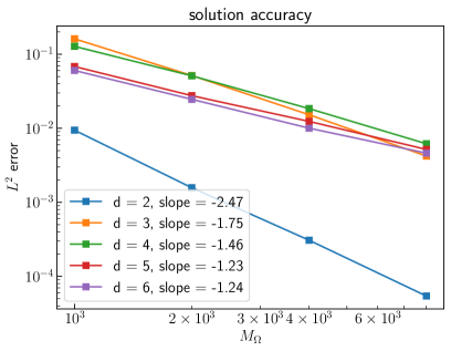
Figure 2: $L^{2}$ test errors of solutions to Problem (37) as a function of the number of collocation points. Left: $\beta=1$; right: $\beta=4$. In both cases, we choose Matérn kernel with $\nu=7/2$. Reported slopes in the legend denote empirical convergence rates.

In the second experiment, we fix $\beta=4$, and choose the Matérn kernel with $\nu=5/2,9/2$ and with lengthscale $\sigma=0.25\sqrt{d}$. Results are shown in Figure 3. Comparing $\nu=5/2,9/2$ and $\nu=7/2$ in the last example, we observe that increasing $\nu$ leads to faster convergence. This is due to the fact that the true solution is smooth. In dimension $d=2$, we can identify the exact convergence rate as $\nu-1$. In all dimensions, the rate is faster than the Monte Carlo rate. We observe that the regularity of the solution softens the effect of the curse of dimensionality, i.e., convergence rates are better in higher dimensions when $\beta$ is smaller.

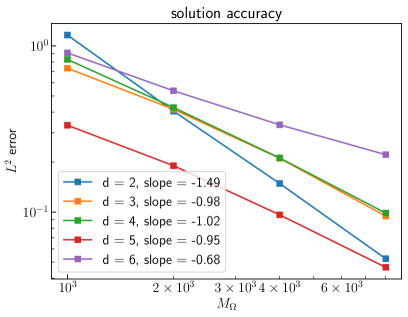
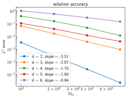
Figure 3: $L^{2}$ test errors of solutions to Problem (37) as a function of the number of collocation points with $\beta=4$. Left: Matérn kernel with $\nu=5/2$; right: Matérn kernel with $\nu=9/2$. Reported slopes in the legend denote empirical convergence rates.

4.2 Parametric PDEs

We consider a parametric version of the linear ($\tau=0$) darcy flow problem in Example 2.1:

(38) $$\left\{\begin{aligned} -\text{div}\big{(}\exp(a(\mathbf{x},\bm{\theta}))\nabla u\big{)}(\mathbf{x})&=f(\mathbf{x}),&&\mathbf{x}\in\Omega,\\ u(\mathbf{x})&=g(\mathbf{x}),&&\mathbf{x}\in\partial\Omega,\end{aligned}\right.$$

Following the general form Eq. 3, we aim to obtain the solution as a function taking values in the product space $\Upsilon$. Eq. 38 can be rewritten in terms of $\mathbf{s}=(\mathbf{x},\bm{\theta})$ with new forcing terms $\hat{f}$ and $\hat{g}$ depending only on the first coordinate of $\mathbf{s}$

(39) $$\left\{\begin{aligned} -\text{div}_{\mathbf{x}}\big{(}A(\mathbf{s})\nabla_{\mathbf{x}}u(\mathbf{s})\big{)}(\mathbf{s})&=\hat{f}(\mathbf{s})=f(\mathbf{x}),&&\mathbf{s}\in\Upsilon,\\ u(\mathbf{s})&=\hat{g}(\mathbf{s})=g(\mathbf{x}),&&\mathbf{s}\in\partial\Upsilon.\end{aligned}\right.$$

Recall that we defined $\partial\Upsilon=\partial\Omega\times\Theta$. For our numerical example, we let $d=1$ and vary $p$. We set $A(x,\theta)=2+\theta_{0}+\sum_{j=1}^{p}\frac{\theta_{j}}{j^{k}}\sin(\pi x+j)$, $f(x)=x$ and $g(x)=0$, a similar setting as in [15]. We choose $\Omega=[0,1]$, and $\Theta=[0,1]^{p}$, for $p=2,3,\ldots,6$. Note $1\leq A(\mathbf{s})\leq 4$ since the sum is in $[-1,1]$ for all $p$ and $\theta\in\Theta$, matching the setting of Example 3.13.

We sample different $M_{\Omega}$ points uniformly in the interior, and $M_{\partial\Omega}=M_{\Omega}/10$ points uniformly on the boundary of $x$. We do two experiments with different choices of kernel, in the first (Fig. 4, left), a vanilla Gaussian kernel with different length scales for the $x$ and $\theta$ dimension, and with a scaling of the length scale in $\theta$ proportional to $\sqrt{p}$. In the second one (Fig. 4, right), we adapt the Gaussian kernel to the decay in $A(x,\theta)$, by including the decay of $1/j^{k}$ in the norm in $\theta$ space used by the kernel. We see significant improvement in test error using this adaptation in high dimensions, which suggests future research directions of kernel adaptation to the specific form of the PDE. In all cases, we use a cross-validation procedure for hyperparameter tuning and we observe the average $L^{2}$ test error on an independent set of test points for different values of $p$ and $M_{\Omega}$. Since $d=1$ we computed our ground truth solution by numerically integrating Equation Eq. 39 using quadrature.

As mentioned, this problem was also explored by [15], in which sparse multivariate polynomials are used to estimate the solution with a rate independent of the number of parameters, provided the decay of the coefficient functions is large enough (in $\ell^{p}$ for some $0<p<1$). While this assumption is satisfied in this example, our method’s convergence rate greatly depends on the dimension of $\theta$ when the kernel is not adapted to the particular equations and coefficients $A(x,\theta)$. Our results indicate improvement in the dependence of convergence rates on dimension when the kernel is adapted to the regularity of $A$. It remains open whether our kernel based approach (which is not specific to parametric equations) can achieve the same dimension independent convergence rates as the ones in [15] (which apply even in the countably infinite dimensional case and which they refer to as breaking the curse of dimensionality) for parametric elliptic PDEs with rapidly decreasing parametric dependence as specified above (this assumption implies a finite number of effective parameters).

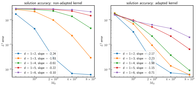
Figure 4: $L^{2}$ test error of solutions to Problem (39) as a function of the number of collocation points. Left: vanilla gaussian kernel; Right: Gaussian kernel adapted to the regularity of $A$. Reported slopes in the legend denote empirical convergence rates.

4.3 High Dimensional HJB Equation

Consider a prototypical HJB equation:

(40) $$(\partial_{t}+\Delta)V(\mathbf{x},t)-|\nabla V(\mathbf{x},t)|^{2} =0$$

$$V(\mathbf{x},T) =g(\mathbf{x})\,,$$

where, $g(\mathbf{x})=\log(\frac{1}{2}+\frac{1}{2}|\mathbf{x}|^{2}),\mathbf{x}\in\mathbb{R}^{d},t\in[0,T]$. We are interested in solving $V(\mathbf{x}_{0},0)$ for some $\mathbf{x}_{0}\in\mathbb{R}^{d}$. We adopt the stochastic differential equation (SDE) formula for representing the solution of the PDEs, following [79, 67]. More specifically, consider the SDE

(41) $$dX_{s}=\sqrt{2}dW_{s},\ X_{0}=\mathbf{x}_{0}\,.$$

We define $Y_{s}=V(X_{s},s),Z_{s}=\sqrt{2}\nabla V(X_{s},s)$. By Ito’s formula, one obtains

(42) $$dY_{s}=\frac{1}{2}|Z_{s}|^{2}ds+Z_{s}\cdot dW_{s}\,.$$

The strategy is to integrate the above SDE backward to $Y_{0}$. An implicit Euler discretization from time $t_{n+1}$ to $t_{n}$ ($\Delta t=t_{n+1}-t_{n}$) leads to the following equation:

(43) $$V(X_{t_{n+1}},t_{n+1})=V(X_{t_{n}},t_{n})+|\nabla V(X_{t_{n}},t_{n})|^{2}\Delta t+\sqrt{2}\nabla V(X_{t_{n}},t_{n})\cdot\xi_{n+1}\sqrt{\Delta t}\,.$$

Algorithmically, we sample $J$ different paths of the forward SDE in (41), namely $X^{(j)}_{t_{n}},1\leq j\leq J$, using the Euler–Maruyama scheme. Then, backward in time, we apply our kernel method, namely to solve the following optimization problem

(44) $$\left\{\begin{aligned} \operatorname*{{\rm minimize}}_{u\in\mathcal{U}}\quad&\|u\|_{\mathcal{U}}\\ {\rm\,s.t.}\quad&u(X^{(j)}_{t_{n}},t_{n})+|\nabla u(X^{(j)}_{t_{n}},t_{n})|^{2}\Delta t+\sqrt{2}\nabla u(X_{t_{n}}^{(j)},t_{n})\cdot\xi_{n+1}\sqrt{\Delta t}=V(X_{t_{n+1}}^{(j)},t_{n+1})\end{aligned}\right.$$

to get the solution $V(\cdot,t_{n})$, assuming $V(\cdot,t_{n+1})$ has been solved. Iterating this process, we end up with the solution $V(\mathbf{x}_{0},0)$. We can understand the algorithm as applying our kernel method iteratively with the sample path as the collocation points.

Experimentally, we consider $d=100$ as in [79, 67]. We aim to solve $V(\mathbf{x}_{0},0)$ for $\mathbf{x}_{0}=0$. The ground truth is $V(\mathbf{x}_{0},0)=4.589992$ provided in [79]. We sample $J=2000$ paths from $\mathbf{x}_{0}$ and choose the inverse quadratic kernel $k(\mathbf{x},\mathbf{y};\sigma)=\left(\frac{\|\mathbf{x}-\mathbf{y}\|^{2}}{2d\sigma^{2}}+1\right)^{-1}\,$. We use the “linearize-then-optimize” approach to compute an approximate solution to (44). The nugget term is set to be $\eta=10^{-3}$. The result is shown in Table 2.

$\sigma$	10	25	50	100	200
Computed solution $V(\mathbf{x}_{0},0)$	5.6042	4.6366	4.6039	4.6021	4.6021
Relative accuracy	22.10%	1.0154%	0.303%	0.2638%	0.2638%

Table 2: Numerical results for the HJB equation (40), computing the quantity $V(\mathbf{x}_{0},0)$.

We observe that a suitable choice of the lengthscale of the kernel is crucial to obtain an accurate solution. Compared to the relative accuracy of $0.171\%$ (reported in [67]) using neural networks (DenseNet like architecture with 4 hidden layers) to solve (43), the accuracy of using kernel methods with a simple quadratic kernel is comparable. Moreover, the lengthscale of the kernel is very large, indicating that the solution behavior of this HJB equation is very smooth; similar “blessings of dimensionality” have been reported and discussed in [67], where they used a constant function (and the terminal function $g$) as ansatz to solve (43) and obtained very high accuracy. Thus, this HJB example in dimension $100$ demonstrates again the trade-off between the smoothness of the solution and the curse of dimensionality.

5 Conclusions

In this paper, we conducted an error analysis of GP and kernel based methods for solving PDEs. We provided convergence rates under the assumptions that (1) the solution belongs to the RKHS which is embedding to some Sobolev space of sufficient regularity, and (2) the underlying forward and inverse PDE operator is stable in corresponding Sobolev spaces.

Our analysis relies on the crucial minimizing norm property of the numerical solution in the kernel/GP methodology. The analysis could be seamlessly generalized to the function class of NNs and other norms such as non-quadratic norms if we can formulate the training process as a minimization problem over the related norm.

We emphasize that our convergence rates hold for the exact minimizer of the minimization problem. In practice, finding such a minimizer algorithmically can be a separate and challenging problem. Our numerical experience suggests that Gauss-Newton iterations usually perform well, and typically, 2-5 iterations are sufficient for convergence. Therefore, we can combine the error analysis in this paper and the fast implementation of the algorithm in [12] to obtain a near-linear complexity solver for nonlinear PDEs with rigorous accuracy guarantee.

It is worth mentioning that this paper focuses only on analyzing the MAP estimator within the GP interpretation. Exploring the posterior distribution of the GP can provide a means for quantifying uncertainty in the solution. In particular, analyzing the posterior contraction is an interesting direction for future research.

Appendix A Sobolev Sampling Inequalities on Manifolds

Below we collect useful sampling inequalities for Sobolev functions defined on smooth manifolds with corners. Following [43, Chs. 1, 16] we consider a smooth, compact Riemannian manifold $\mathcal{M}\subset\mathbb{R}^{d}$ of dimension $k\leq d$ with corners, i.e., a Riemannian manifold with a smooth structure with corners; see [43, Ch. 16]. On such a manifold we define the natural geodesic distance

$$\rho_{\mathcal{M}}:\mathcal{M}\times\mathcal{M}\to\mathbb{R},\qquad\rho_{\mathcal{M}}(x,y):=\inf\int_{0}^{1}\|\dot{\ell}(t)\|dt,$$

where the infimum is taken over all piecewise smooth paths $\ell:[0,1]\mapsto\mathcal{M}$ satisfying the boundary conditions $\ell(0)=x$ and $\ell(1)=y$, and $\|\dot{\ell}(t)\|$ is the length of the tangent vector $\dot{\ell}(T)$ under the Riemannian metric.

Following [29] (see also [76, Sec. 4.3]) we further consider the Sobolev spaces $H^{k}(\mathcal{M})$ of functions defined on $\mathcal{M}$ as follows: Let $\mathcal{A}=\{M_{j},\Psi_{j}\}_{j=1}^{N}$ be an atlas for $\mathcal{M}$ and let $\{\kappa_{j}\}$ be a partition of unity of $\mathcal{M}$, subordinate to $M_{j}$. Then given functions $u:\mathcal{M}\to\mathbb{R}$ we define the Sobolev norms and the associated Sobolev spaces $H^{s}(\mathcal{M})$ as

$$H^{s}(\mathcal{M}):=\{u:\mathcal{M}\to\mathbb{R}\mid\|u\|_{H^{s}(\mathcal{M})}<+\infty\},\qquad\|u\|_{H^{s}(\mathcal{M})}:=\left(\sum_{j=1}^{N}\|\pi_{j}(u)\|_{H^{s}(\Xi_{j})}^{2}\right)^{1/2},$$

where the maps $\pi_{j}$ are defined as

$$\pi_{j}(f):=\left\{\begin{aligned} &\kappa_{j}(f(\Psi_{j}^{-1}(y))),&&\text{if }y\in\Psi_{j}(M_{j}),\\ &0&&\text{otherwise.}\end{aligned}\right.$$

and the sets $\Xi_{j}$ are given by

$$\Xi_{j}:=\left\{\begin{aligned} &\mathbb{R}^{k}&&\text{if $\Psi_{j}$ is an interior chart,}\\ &\{(x_{1},\dots,x_{k})\in\mathbb{R}^{k}|x_{1}\geq 0\}&&\text{if $\Psi_{j}$ is a boundary chart,}\\ &\{(x_{1},\dots,x_{k})\in\mathbb{R}^{k}|x_{1}\geq 0,\dots,x_{k}\geq 0\}&&\text{if $\Psi_{j}$ is a corner chart.}\\ \end{aligned}\right.$$

Put simply, the Sobolev spaces $H^{s}(\mathcal{M})$ are functions on $\mathcal{M}$ that, locally after the flattening of the manifold belong to the standard Sobolev spaces $H^{s}$. With these notions at hand we then recall the following result of [29], which was proven by those authors for smooth embedded manifolds without boundary or corners. However, a brief investiation of the proof of that result reveals that it can immediately be generalized to our setting with manifolds with corners. In fact, the idea of the proof is to use the atlas to locally flatten the manifold and apply classic sampling theorems such as [2, Thm. 4.1] on each patch. The only difference in the case of manifolds with corners is that the patches do not only map to $\mathbb{R}^{k}$ but rather to the subspaces $\Xi_{j}$ depending on whether the corresponding chart is an interior, boundary, or corner chart.

Proposition A.1 ([29, Lem. 10]).

Suppose $\mathcal{M}\subset\mathbb{R}^{d}$ is a smooth, compact, Riemannian manifold with corners, of dimension $k$ and let $s>k/2$ and $r\in\mathbb{N}$ satisfy $0\leq r\leq\lceil s\rceil-1$. Let $X\subset\mathcal{M}$ be a discrete set with mesh norm $h_{\mathcal{M}}$ defined as

$$h_{\mathcal{M}}:=\sup_{x^{\prime}\in\mathcal{M}}\inf_{x\in X}\rho_{\mathcal{M}}(x,x^{\prime}).$$

Then there is a constant $h_{0}>0$ depending only on $\mathcal{M}$ such that if $h_{\mathcal{M}}<h_{0}$ and if $u\in H^{s}(\mathcal{M})$ satisfies $u|_{X}=0$ then

$$\|u\|_{H^{r}(\mathcal{M})}\leq Ch_{\mathcal{M}}^{s-r}\|u\|_{H^{s}(\mathcal{M})}.$$

Here $C>0$ is a constant independent of $h_{\mathcal{M}}$ and $u$.

Appendix B Bounds on Fill Distances

This section collects a result from [66] for bounding the fill-in distance for randomly distributed points on a manifold.

Assume $(\mathcal{M},\rho)$ is a metric space, and $\mu$ is a finite positive Borel measure supported on $\mathcal{M}$. Let $X=\{x_{1},...,x_{N}\}$ be a set of $N$ points, independently and randomly drawn from $\mu$. Define the fill-in distance

(45) $$h_{\mathcal{M}}=\sup_{x^{\prime}\in\mathcal{M}}\inf_{x\in X}\rho(x,x^{\prime})\,.$$

Then, [66, Thm. 2.1] implies the following:

Proposition B.1.

Suppose $\Phi$ is a continuous non-negative strictly increasing function on $(0,\infty)$ satisfying $\Phi(r)\to 0$ as $r\to 0^{+}$. If there exists a positive number $r_{0}$ such that $\mu(B(x,r))\geq\Phi(r)$ holds for all $x\in\mathcal{M}$ and every $r<r_{0}$, then there exist positive constants $c_{1},c_{2},c_{3}$ and $\alpha_{0}$ such that for any $\alpha>\alpha_{0}$, we have

(46) $$\mathbb{P}\left[h_{\mathcal{M}}\geq c_{1}\Phi^{-1}\left(\frac{\alpha\log N}{N}\right)\right]\leq c_{2}N^{1-c_{3}\alpha}.$$

We use this proposition to prove Proposition 3.14.

Proof B.2 (Proof of Proposition 3.14).

We apply Proposition B.1. For the bounded domain $\Omega\subset\mathbb{R}^{d}$, we know that there exists a constant $C$ such that $\Phi(r)=Cr^{d}$ will satisfy the assumption in Proposition B.1. Moreover, we choose $\alpha$ such that $c_{2}M_{\Omega}^{1-c_{3}\alpha}\leq\delta$. This implies that $\alpha\geq\frac{1}{c_{3}\log M_{\Omega}}\log(c_{2}M_{\Omega}/\delta)$. Pick $\alpha=\frac{C^{\prime}}{c_{3}\log M_{\Omega}}\log(c_{2}M_{\Omega}/\delta)$ for some $C^{\prime}\geq 1$ such that $\alpha\geq\alpha_{0}$. Then Proposition B.1 shows that with probability at least $1-\delta$,

$$h_{\Omega}\leq c_{1}\Phi^{-1}\left(\frac{\alpha\log M_{\Omega}}{M_{\Omega}}\right)\leq C^{\prime\prime}\left(\frac{\log(M_{\Omega}/\delta)}{M_{\Omega}}\right)^{1/d},$$

where $C^{\prime\prime}$ is a constant independent of $M_{\Omega}$ and $\delta$. The bound on $h_{\partial\Omega}$ can be proved similarly by choosing $\Phi(r)=Cr^{d-1}$.

Appendix C The Choice of Nugget Terms

For numerical stability, we add a diagonal adaptive nugget term to the kernel matrix in our computation such that

$$u^{\ell+1}(x)=K(x,{\bm{\phi}}^{l})[K({\bm{\phi}}^{l},{\bm{\phi}}^{l})+\eta\mathrm{diag}(K({\bm{\phi}}^{l},{\bm{\phi}}^{l}))]^{-1}\begin{pmatrix}\left(f-u^{\ell}+\mathcal{P}^{\prime}(u^{\ell})u^{\ell}\right)|_{\mathbf{s}_{\Omega}}\\ \left(g-u^{\ell}+\mathcal{B}^{\prime}(u^{\ell})u^{\ell}\right)|_{\mathbf{s}_{\partial\Omega}}\end{pmatrix}$$

Typically $\eta=10^{-10}$. This nugget term is similar to the adaptive nugget term proposed in [11]. It is much more effective than the naive choice of $K({\bm{\phi}}^{l},{\bm{\phi}}^{l})+\eta I$, since the conditioning of the interior block and the boundary block in the kernel matrix differs dramatically.

References

- [1] B. O. Almroth, P. Stern, and F. A. Brogan, Automatic choice of global shape functions in structural analysis, Aiaa Journal, 16 (1978), pp. 525–528.
- [2] R. Arcangéli, M. C. López de Silanes, and J. J. Torrens, An extension of a bound for functions in Sobolev spaces, with applications to -spline interpolation and smoothing, Numerische Mathematik, 107 (2007), pp. 181–211.
- [3] I. Babuška and J. Osborn, Can a finite element method perform arbitrarily badly?, Mathematics of computation, 69 (2000), pp. 443–462.
- [4] P. Batlle, M. Darcy, B. Hosseini, and H. Owhadi, Kernel methods are competitive for operator learning, arXiv preprint arXiv:2304.13202, (2023).
- [5] J. Beck, R. Tempone, F. Nobile, and L. Tamellini, On the optimal polynomial approximation of stochastic PDEs by Galerkin and collocation methods, Mathematical Models and Methods in Applied Sciences, 22 (2012), p. 1250023.
- [6] A. Berlinet and C. Thomas-Agnan, Reproducing kernel Hilbert spaces in probability and statistics, Springer Science & Business Media, 2011.
- [7] V. I. Bogachev, Gaussian measures, American Mathematical Society, 1998.
- [8] K. Böhmer and R. Schaback, A nonlinear discretization theory, Journal of computational and applied mathematics, 254 (2013), pp. 204–219.
- [9] K. Böhmer and R. Schaback, A nonlinear discretization theory for meshfree collocation methods applied to quasilinear elliptic equations, ZAMM-Journal of Applied Mathematics and Mechanics/Zeitschrift für Angewandte Mathematik und Mechanik, 100 (2020), p. e201800170.
- [10] J. Chen, F. Schäfer, J. Huang, and M. Desbrun, Multiscale cholesky preconditioning for ill-conditioned problems, ACM Transactions on Graphics (TOG), 40 (2021), pp. 1–13.
- [11] Y. Chen, B. Hosseini, H. Owhadi, and A. M. Stuart, Solving and learning nonlinear PDEs with Gaussian processes, Journal of Computational Physics, 447 (2021), p. 110668.
- [12] Y. Chen, H. Owhadi, and F. Schäfer, Sparse Cholesky factorization for solving nonlinear PDEs via Gaussian processes, arXiv preprint arXiv:2304.01294, (2023).
- [13] Y. Chen, H. Owhadi, and A. Stuart, Consistency of empirical Bayes and kernel flow for hierarchical parameter estimation, Mathematics of Computation, (2021).
- [14] K. C. Cheung, L. Ling, and R. Schaback, -convergence of least-squares kernel collocation methods, SIAM Journal on Numerical Analysis, 56 (2018), pp. 614–633.
- [15] A. Chkifa, A. Cohen, R. DeVore, and C. Schwab, Sparse adaptive taylor approximation algorithms for parametric and stochastic elliptic PDEs, ESAIM: Mathematical Modelling and Numerical Analysis, 47 (2012), pp. 253–280.
- [16] A. Chkifa, A. Cohen, and C. Schwab, High-dimensional adaptive sparse polynomial interpolation and applications to parametric PDEs, Foundations of Computational Mathematics, 14 (2014), pp. 601–633.
- [17] O. A. Chkrebtii, D. A. Campbell, B. Calderhead, and M. A. Girolami, Bayesian solution uncertainty quantification for differential equations, Bayesian Analysis, 11 (2016), pp. 1239–1267.
- [18] I. Cialenco, G. E. Fasshauer, and Q. Ye, Approximation of stochastic partial differential equations by a kernel-based collocation method, International Journal of Computer Mathematics, 89 (2012), pp. 2543–2561.
- [19] J. Cockayne, C. Oates, T. Sullivan, and M. Girolami, Probabilistic numerical methods for PDE-constrained Bayesian inverse problems, in AIP Conference Proceedings, vol. 1853, 2017, p. 060001.
- [20] J. Cockayne, C. J. Oates, T. J. Sullivan, and M. Girolami, Bayesian probabilistic numerical methods, SIAM Review, 61 (2019), pp. 756–789.
- [21] A. Cohen and R. DeVore, Approximation of high-dimensional parametric PDEs, Acta Numerica, 24 (2015), pp. 1–159.
- [22] A. Cohen, R. DeVore, and C. Schwab, Convergence rates of best -term Galerkin approximations for a class of elliptic sPDEs, Foundations of Computational Mathematics, 10 (2010), pp. 615–646.
- [23] M. Darcy, B. Hamzi, G. Livieri, H. Owhadi, and P. Tavallali, One-shot learning of stochastic differential equations with data adapted kernels, Physica D: Nonlinear Phenomena, 444 (2023), p. 133583.
- [24] T. De Ryck and S. Mishra, Error analysis for physics-informed neural networks (pinns) approximating kolmogorov PDEs, Advances in Computational Mathematics, 48 (2022), pp. 1–40.
- [25] R. P. Feynman, Cargo cult science, in The art and science of analog circuit design, Elsevier, 1998, pp. 55–61.
- [26] B. Fornberg and N. Flyer, Solving PDEs with radial basis functions, Acta Numerica, 24 (2015), pp. 215–258.
- [27] C. Franke and R. Schaback, Convergence order estimates of meshless collocation methods using radial basis functions, Advances in computational mathematics, 8 (1998), pp. 381–399.
- [28] C. Franke and R. Schaback, Solving partial differential equations by collocation using radial basis functions, Applied Mathematics and Computation, 93 (1998), pp. 73–82.
- [29] E. Fuselier and G. B. Wright, Scattered data interpolation on embedded submanifolds with restricted positive definite kernels: Sobolev error estimates, SIAM Journal on Numerical Analysis, 50 (2012), pp. 1753–1776.
- [30] R. G. Ghanem and P. D. Spanos, Stochastic finite elements: a spectral approach, Dover Publications, 2003.
- [31] P. Giesl and H. Wendland, Meshless collocation: Error estimates with application to dynamical systems, SIAM Journal on Numerical Analysis, 45 (2007), pp. 1723–1741.
- [32] D. Gilbarg and N. S. Trudinger, Elliptic Partial Differential Equations of second order, vol. 224, Springer, 1977.
- [33] T. G. Grossmann, U. J. Komorowska, J. Latz, and C.-B. Schönlieb, Can physics-informed neural networks beat the finite element method?, arXiv preprint arXiv:2302.04107, (2023).
- [34] M. D. Gunzburger, C. G. Webster, and G. Zhang, Stochastic finite element methods for partial differential equations with random input data, Acta Numerica, 23 (2014), pp. 521–650.
- [35] J. S. Hesthaven, G. Rozza, B. Stamm, et al., Certified reduced basis methods for parametrized partial differential equations, vol. 590, Springer, 2016.
- [36] E. J. Kansa, Multiquadrics—a scattered data approximation scheme with applications to computational fluid-dynamics—i surface approximations and partial derivative estimates, Computers & Mathematics with applications, 19 (1990), pp. 127–145.
- [37] E. J. Kansa, Multiquadrics—a scattered data approximation scheme with applications to computational fluid-dynamics—ii solutions to parabolic, hyperbolic and elliptic partial differential equations, Computers & mathematics with applications, 19 (1990), pp. 147–161.
- [38] R. Kempf, H. Wendland, and C. Rieger, Kernel-based reconstructions for parametric PDEs, in IWMMPDE 2017: Meshfree Methods for Partial Differential Equations IX 9, Springer, 2019, pp. 53–71.
- [39] M. C. Kennedy and A. O’Hagan, Bayesian calibration of computer models, Journal of the Royal Statistical Society: Series B (Statistical Methodology), 63 (2001), pp. 425–464.
- [40] F. M. Larkin, Gaussian measure in Hilbert space and applications in numerical analysis, Journal of Mathematics, 2 (1972).
- [41] O. Le Maître and O. M. Knio, Spectral methods for uncertainty quantification: with applications to computational fluid dynamics, Springer Science & Business Media, 2010.
- [42] J. Lee, Y. Bahri, R. Novak, S. S. Schoenholz, J. Pennington, and J. Sohl-Dickstein, Deep neural networks as Gaussian processes, arXiv preprint arXiv:1711.00165, (2017).
- [43] J. M. Lee, Introduction to Smooth Manifolds, Springer, 2012.
- [44] Z. Li, N. Kovachki, K. Azizzadenesheli, K. Bhattacharya, A. Stuart, and A. Anandkumar, Fourier neural operator for parametric partial differential equations, in International Conference on Learning Representations, 2020.
- [45] D. Long, N. Mrvaljevic, S. Zhe, and B. Hosseini, A kernel approach for pde discovery and operator learning, arXiv preprint arXiv:2210.08140, (2022).
- [46] D. Long, Z. Wang, A. Krishnapriyan, R. Kirby, S. Zhe, and M. Mahoney, Autoip: A united framework to integrate physics into gaussian processes, in International Conference on Machine Learning, PMLR, 2022, pp. 14210–14222.
- [47] L. Lu, P. Jin, G. Pang, Z. Zhang, and G. E. Karniadakis, Learning nonlinear operators via DeepONet based on the universal approximation theorem of operators, Nature Machine Intelligence, 3 (2021), pp. 218–229.
- [48] Y. Lu, H. Chen, J. Lu, L. Ying, and J. Blanchet, Machine learning for elliptic PDEs: fast rate generalization bound, neural scaling law and minimax optimality, arXiv preprint arXiv:2110.06897, (2021).
- [49] D. J. Lucia, P. S. Beran, and W. A. Silva, Reduced-order modeling: new approaches for computational physics, Progress in aerospace sciences, 40 (2004), pp. 51–117.
- [50] W. McLean, Strongly elliptic systems and boundary integral equations, Cambridge university press, 2000.
- [51] J. M. Melenk, On n-widths for elliptic problems, Journal of mathematical analysis and applications, 247 (2000), pp. 272–289.
- [52] R. Meng and X. Yang, Sparse Gaussian processes for solving nonlinear PDEs, arXiv preprint arXiv:2205.03760, (2022).
- [53] C. Mou, X. Yang, and C. Zhou, Numerical methods for mean field games based on Gaussian processes and Fourier features, Journal of Computational Physics, 460 (2022), p. 111188.
- [54] K. Muandet, K. Fukumizu, B. Sriperumbudur, B. Schölkopf, et al., Kernel mean embedding of distributions: A review and beyond, Foundations and Trends® in Machine Learning, 10 (2017), pp. 1–141.
- [55] R. M. Neal, Priors for infinite networks, Bayesian learning for neural networks, (1996), pp. 29–53.
- [56] F. Nobile, R. Tempone, and C. G. Webster, An anisotropic sparse grid stochastic collocation method for partial differential equations with random input data, SIAM Journal on Numerical Analysis, 46 (2008), pp. 2411–2442.
- [57] F. Nobile, R. Tempone, and C. G. Webster, A sparse grid stochastic collocation method for partial differential equations with random input data, SIAM Journal on Numerical Analysis, 46 (2008), pp. 2309–2345.
- [58] A. K. Noor and J. M. Peters, Reduced basis technique for nonlinear analysis of structures, Aiaa journal, 18 (1980), pp. 455–462.
- [59] H. Owhadi, Bayesian numerical homogenization, Multiscale Modeling & Simulation, 13 (2015), pp. 812–828.
- [60] H. Owhadi, Do ideas have shape? idea registration as the continuous limit of artificial neural networks, Physica D: Nonlinear Phenomena, 444 (2023), p. 133592.
- [61] H. Owhadi and C. Scovel, Operator-Adapted Wavelets, Fast Solvers, and Numerical Homogenization: From a Game Theoretic Approach to Numerical Approximation and Algorithm Design, Cambridge University Press, 2019.
- [62] H. Owhadi and G. R. Yoo, Kernel flows: from learning kernels from data into the abyss, Journal of Computational Physics, 389 (2019), pp. 22–47.
- [63] A. Pinkus, N-widths in Approximation Theory, vol. 7, Springer Science & Business Media, 2012.
- [64] M. Raissi, P. Perdikaris, and G. E. Karniadakis, Numerical Gaussian processes for time-dependent and nonlinear partial differential equations, SIAM Journal on Scientific Computing, 40 (2018), pp. A172–A198.
- [65] M. Raissi, P. Perdikaris, and G. E. Karniadakis, Physics-informed neural networks: A deep learning framework for solving forward and inverse problems involving nonlinear partial differential equations, Journal of Computational Physics, 378 (2019), pp. 686–707.
- [66] A. Reznikov and E. B. Saff, The covering radius of randomly distributed points on a manifold, International Mathematics Research Notices, 2016 (2016), pp. 6065–6094.
- [67] L. Richter, L. Sallandt, and N. Nüsken, Solving high-dimensional parabolic PDEs using the tensor train format, arXiv preprint arXiv:2102.11830, (2021).
- [68] S. Särkkä, Linear operators and stochastic partial differential equations in gaussian process regression, in International Conference on Artificial Neural Networks, Springer, 2011, pp. 151–158.
- [69] R. Schaback, All well-posed problems have uniformly stable and convergent discretizations, Numerische Mathematik, 132 (2016), pp. 597–630.
- [70] R. Schaback and H. Wendland, Kernel techniques: from machine learning to meshless methods, Acta numerica, 15 (2006), p. 543.
- [71] F. Schäfer, M. Katzfuss, and H. Owhadi, Sparse cholesky factorization by Kullback–Leibler minimization, SIAM Journal on Scientific Computing, 43 (2021), pp. A2019–A2046.
- [72] F. Schäfer, T. J. Sullivan, and H. Owhadi, Compression, inversion, and approximate pca of dense kernel matrices at near-linear computational complexity, Multiscale Modeling & Simulation, 19 (2021), pp. 688–730.
- [73] B. Scholkopf and A. J. Smola, Learning with kernels: support vector machines, regularization, optimization, and beyond, MIT Press, 2018.
- [74] Y. Shin, J. Darbon, and G. E. Karniadakis, On the convergence of physics informed neural networks for linear second-order elliptic and parabolic type PDEs, arXiv preprint arXiv:2004.01806, (2020).
- [75] L. P. Swiler, M. Gulian, A. L. Frankel, C. Safta, and J. D. Jakeman, A survey of constrained Gaussian process regression: Approaches and implementation challenges, Journal of Machine Learning for Modeling and Computing, 1 (2020).
- [76] M. Taylor, Partial differential equations I: Basic theory, Springer Science & Business Media, 2013.
- [77] A. W. van der Vaart and J. H. van Zanten, Reproducing Kernel Hilbert Spaces of Gaussian priors, in Pushing the limits of contemporary statistics: contributions in honor of Jayanta K. Ghosh, Institute of Mathematical Statistics, 2008, pp. 200–222.
- [78] J. Wang, J. Cockayne, O. Chkrebtii, T. J. Sullivan, C. Oates, et al., Bayesian numerical methods for nonlinear partial differential equations, Statistics and Computing, 31 (2021), pp. 1–20.
- [79] E. Weinan, J. Han, and A. Jentzen, Deep learning-based numerical methods for high-dimensional parabolic partial differential equations and backward stochastic differential equations, Communications in Mathematics and Statistics, 5 (2017), pp. 349–380.
- [80] E. Weinan and B. Yu, The deep ritz method: a deep learning-based numerical algorithm for solving variational problems, Communications in Mathematics and Statistics, 6 (2018), pp. 1–12.
- [81] H. Wendland, Scattered Data Approximation, Cambridge University Press, 2004.
- [82] C. K. I. Williams and C. E. Rasmussen, Gaussian Processes for Machine Learning, The MIT Press, 2006.
- [83] A. G. Wilson, Z. Hu, R. Salakhutdinov, and E. P. Xing, Deep kernel learning, in Artificial Intelligence and Statistics, PMLR, 2016, pp. 370–378.
- [84] D. Xiu, Numerical Methods for Stochastic Computations: A Spectral Method Approach, Princeton University Press, 2010.
- [85] Q. Ye, Kernel-based methods for stochastic partial differential equations, arXiv preprint arXiv:1303.5381, (2013).